1

Stochastic Trees and the StoTree Modeling

Environment: Models and Software for Medical Decision

Analysis

Gordon B. Hazen

Northwestern University

June 2001

Abstract

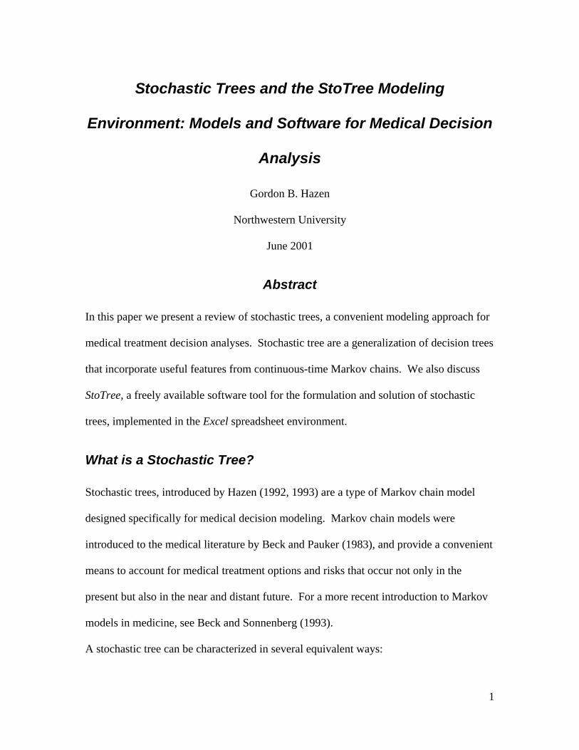
In this paper we present a review of stochastic trees, a convenient modeling approach for

medical treatment decision analyses. Stochastic tree are a generalization of decision trees

that incorporate useful features from continuous-time Markov chains. We also discuss

StoTree, a freely available software tool for the formulation and solution of stochastic

trees, implemented in the Excel spreadsheet environment.

What is a Stochastic Tree?

Stochastic trees, introduced by Hazen (1992, 1993) are a type of Markov chain model

designed specifically for medical decision modeling. Markov chain models were

introduced to the medical literature by Beck and Pauker (1983), and provide a convenient

means to account for medical treatment options and risks that occur not only in the

present but also in the near and distant future. For a more recent introduction to Markov

models in medicine, see Beck and Sonnenberg (1993).

A stochastic tree can be characterized in several equivalent ways:

2

• As a continuous-time Markov chain with chance and decision nodes added

• As a decision tree with stochastic transitions added

• As a multi-state DEALE model (Beck, Kassirer and Pauker 1982)

• As a continuous-time version of a Markov cycle tree (Hollenberg 1984)

We discuss both the graphical and the computational features of stochastic trees.

Graphical features of stochastic trees

The stochastic tree in Figure 1 is a model of risk of recurrent stroke following carotid

endarterectomy, based on Matchar and Pauker (1986). Nodes such as “Well”, “Stroke”,

and so on, depict health states. A health state can have incremental impact or

instantaneous impact, depending on the type of arrows emanating from it. Wavy arrows

emanate from incremental impact states such as “Well” or “Post Big Stroke”, and

indicate that the incremental impact state is occupied for a duration that is uncertain but

dependent on the rates that label the arrows. For example, the state “Well” is occupied

until either a stroke occurs (the average stroke rate is ms = 0.05/yr.) or death occurs due

to other causes (the rate is m0 + me = 0.0111/yr. + 0.065/yr = 0.0761/yr), at which time

transition occurs to either “Stroke” or “Dead”, respectively. Incremental impact states act

just like nodes in a transition diagram for a continuous-time Markov chain. Sometimes

we will call such nodes stochastic nodes, and will refer to the associated arcs as

stochastic arcs.

Straight arrows emanate from instantaneous impact states, and indicate that transition

occurs immediately to a subsequent state with probability equal to the probability labeling

the corresponding arrow. For example, in Figure 1, “Stroke” is an instantaneous impact

state that leads with probability pb = 2/3 to the state “Big Stroke” and probability 1−pb =

3

1/3 to the state “Small Stoke”. Instantaneous impact states act just like chance nodes in a

decision tree. We will therefore call such nodes chance nodes, and will refer to the

associated arcs as chance arcs.

Transition cycles are also allowed in stochastic trees. In Figure 1, transition cycles are

depicted using phantom nodes, nodes with dashed borders that are copies of other nodes

in the stochastic tree. For example, the second “Big Stroke” node in the model has a

dashed border, indicating that it is identical to the previous “Big Stroke” node. The net

effect is that with rate pb⋅ms, transition can occur from state “Post Big Stroke” back to

previously visited state “Big Stroke”. There is also a phantom node “Stroke”, which

allows transition from state “Post Small Stroke” to the previously visited state “Stroke”.

The stochastic tree diagram in Figure 1 was produced inside an Excel workbook using the

Visual Basic software StoTree developed by Hazen. We discuss this software in more

detail below.

4

1.828

7.9331.134

2.971

6.646 6.646

ms = 0.05 /yrpe = 0.38pb = 0.6667me = 0.065 /yrm0 = 0.0111 /yr

qPBS = 0.2qPSS = 0.8

.

m0 + me

ms

pb

m0 + me

m0 + me

1 - pb

ms

pe

1 - pe

pb ms

Well

Stroke

Small Stroke Post Small Stroke

Big Stroke

Post Big Stroke

Dead

Dead

Dead

Dead

Big Stroke

Stroke

Figure 1: A stochastic tree model of recurrent stroke following carotid endarterectomy, based on

Matchar and Pauker (1986). This model was formulated in an Excel spreadsheet using the

StoTree software.

Computational features of stochastic trees

Mean quality-adjusted lifetime can be computed easily in stochastic trees using rollback

procedures not unlike those for decision trees. As noted by Hazen (1992), these rollback

procedures arise from the equivalence

λ2

λ1

λ3

x y2

y1

y3

= λ

p3

p2

p1

x

y3

y1

y2...

λ = ∑λi i pi = λi/λ

5

known as superposition/ decomposition in the stochastic processes literature. This

diagram indicates that multiple competing transitions out of a state x to states y1, y2, y3 at

competing rates λ1, λ2, λ3, are equivalent to a single transition out of x at rate λ = λ1 + λ2

+ λ3, followed by an immediate transition to y1, y2, or y3 with probabilities p1, p2, p3,

where pi = λi/λ. This equivalence leads to the following rollback procedure: If L(x) is

mean quality adjusted duration beginning at state x, then

∑ ∑∑λ

λ+=+

λ⋅=

ii i

i iii

)y(L)x(v)y(Lp1)x(v)x(L

Here L(yi) is mean quality-adjusted lifetime beginning in state yi, and v(x) is the quality

adjustment for time spent in state x.

The StoTree software implements this rollback procedure and places the resulting

formulas for mean quality-adjusted durations directly into the Excel spreadsheet. The

rollback results for the Matchar and Pauker example from Figure 1 are displayed in

Figure 2.

6

1.828

7.9331.134

2.971

6.646 6.646

ms = 0.05 /yrpe = 0.38pb = 0.6667me = 0.065 /yrm0 = 0.0111 /yr

qPBS = 0.2qPSS = 0.8

.

m0 + me

ms

pb

m0 + me

m0 + me

1 - pb

ms

pe

1 - pe

pb ms

Well

Stroke

Small Stroke Post Small Stroke

Big Stroke

Post Big Stroke

Dead

Dead

Dead

Dead

Big Stroke

Stroke

Figure 2: Rollback results for the Matchar and Pauker model from Figure 1. The quality

adjustments for the Well, Post Big Stroke, and Post Small Stroke states are 1, qPBS = 0.2, and

qPSS = 0.8. Mean quality adjusted lifetime beginning in the Well state is 7.933 years. Other

states are labeled with mean quality adjusted lifetimes beginning at those states.

Factored Stochastic Trees

We consider a Markov model discussed by Beck and Sonnenberg (1993), whose essential

characteristics are as follows:

• A 42-year old man received a kidney transplant 18 months ago. Normal kidney

function has been maintained under immunosuppressive therapy.Recently, two

synchronous melanomas appeared and required wide resectionShould

immunosuppressive therapy be continued?

–Continuation increases chance of another possibly lethal melanoma

7

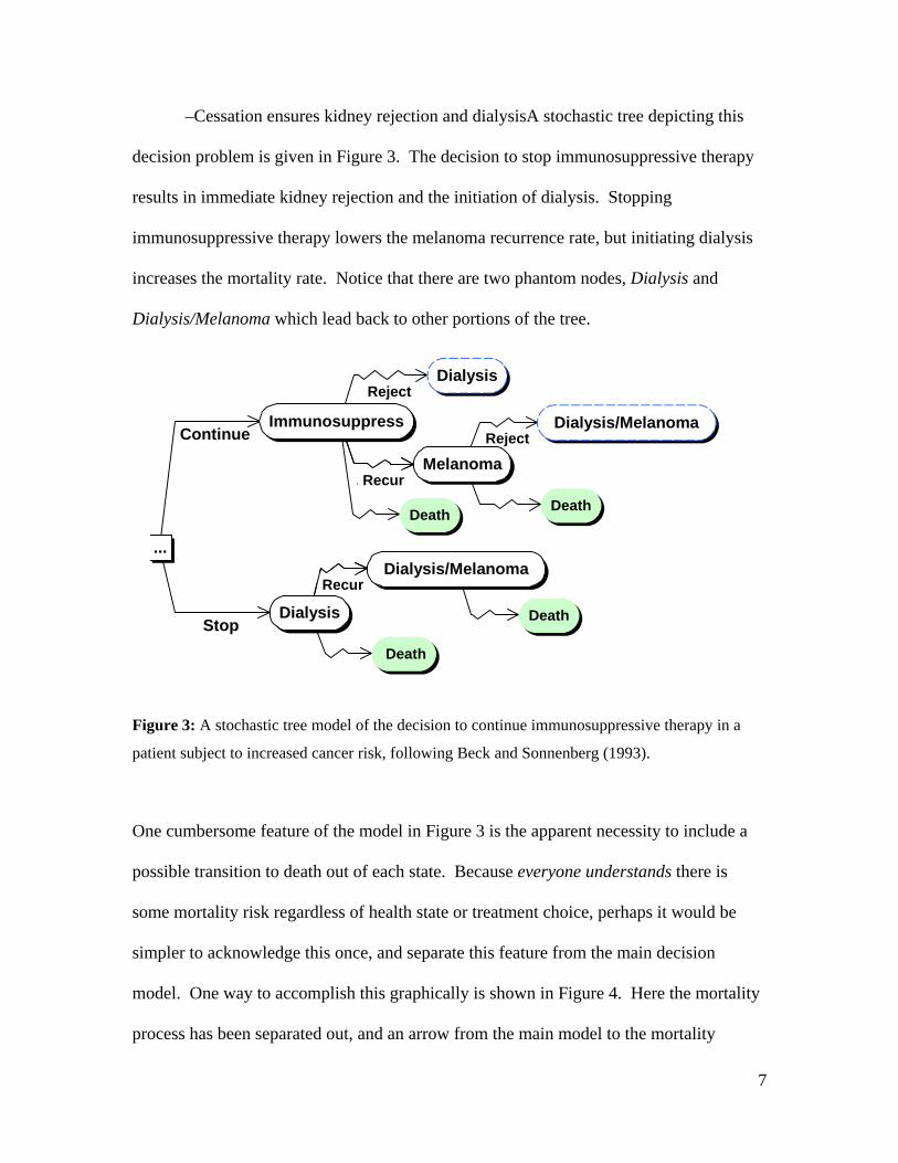
–Cessation ensures kidney rejection and dialysisA stochastic tree depicting this

decision problem is given in Figure 3. The decision to stop immunosuppressive therapy

results in immediate kidney rejection and the initiation of dialysis. Stopping

immunosuppressive therapy lowers the melanoma recurrence rate, but initiating dialysis

increases the mortality rate. Notice that there are two phantom nodes, Dialysis and

Dialysis/Melanoma which lead back to other portions of the tree.

Stop

Continue

............Recur

............

Reject

Reject

Recur

...

Dialysis

Dialysis/Melanoma

Immunosuppress

Melanoma

Death

Death Death

Dialysis

Death

Dialysis/Melanoma

Figure 3: A stochastic tree model of the decision to continue immunosuppressive therapy in a

patient subject to increased cancer risk, following Beck and Sonnenberg (1993).

One cumbersome feature of the model in Figure 3 is the apparent necessity to include a

possible transition to death out of each state. Because everyone understands there is

some mortality risk regardless of health state or treatment choice, perhaps it would be

simpler to acknowledge this once, and separate this feature from the main decision

model. One way to accomplish this graphically is shown in Figure 4. Here the mortality

process has been separated out, and an arrow from the main model to the mortality

8

process has been added to indicate that mortality rate can be affected by the state of the

main model. The mortality process and the processes in the main model proceed in

parallel. We say we have factored out mortality from the main model, and we call the

result a factored stochastic tree. An advantage of factoring out mortality is that the

structure of the main model can be more easily discerned once all the death transitions

have been removed.

Alive Dead

Mortality Mortality Rate

Stop

Continue

Reject

Reject

Recur

Recur

...

Dialysis

Dialysis/Melanoma

Immunosuppress

Melanoma

Dialysis/Melanoma

Dialysis

Figure 4: Factoring mortality out of the Beck and Sonnenberg model of Figure 3. Mortality rate

depends on the state of the main model.

However, once we are aware of the possibility of factoring, there is no reason to limit

ourselves to factoring out mortality. In addition to mortality, the main model has three

other processes that proceed in parallel:

• the cancer recurrence process

• the kidney rejection process

9

• the initial process of deciding whether to stop immunosuppressive therapy.

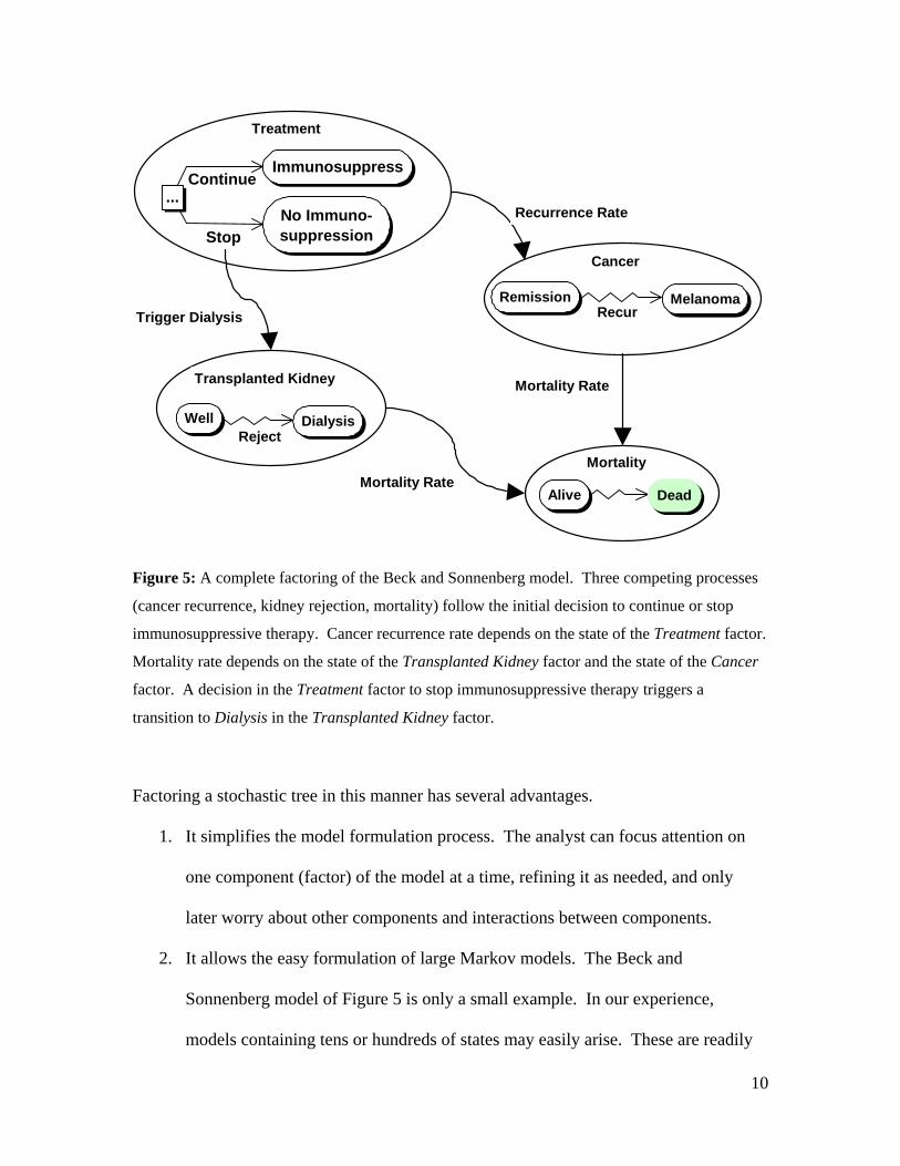
If we factor out these processes as well, we obtain the factored stochastic tree of Figure 5.

The figure depicts the component processes and also how they influence each other. In

addition to the influences on mortality rate, we see that the decision to continue or stop

immunosuppressive therapy influences cancer recurrence rate. There is also a triggering

influence: the decision to stop immunosuppressive therapy triggers an immediate

transition from Well to Dialysis in the Transplanted Kidney factor.

It is important to remember that in a factored stochastic tree, the factors depict processes

that are proceeding in parallel. So any combination of states, one from each factor, may

in principal occur. For example, the Dialysis/Melanoma state in Figure 4 may seem

absent from the factored tree in Figure 5, but it is represented implicitly by the

combination of states Dialysis in the Transplanted Kidney factor, and Melanoma in the

Cancer factor.

10

RejectWell Dialysis

Transplanted Kidney

RecurRemission Melanoma

CancerStop

Continue...

No Immuno-suppression

Immunosuppress

Treatment

Alive Dead

Mortality

Trigger Dialysis

Mortality Rate

Mortality Rate

Recurrence Rate

Figure 5: A complete factoring of the Beck and Sonnenberg model. Three competing processes

(cancer recurrence, kidney rejection, mortality) follow the initial decision to continue or stop

immunosuppressive therapy. Cancer recurrence rate depends on the state of the Treatment factor.

Mortality rate depends on the state of the Transplanted Kidney factor and the state of the Cancer

factor. A decision in the Treatment factor to stop immunosuppressive therapy triggers a

transition to Dialysis in the Transplanted Kidney factor.

Factoring a stochastic tree in this manner has several advantages.

1. It simplifies the model formulation process. The analyst can focus attention on

one component (factor) of the model at a time, refining it as needed, and only

later worry about other components and interactions between components.

2. It allows the easy formulation of large Markov models. The Beck and

Sonnenberg model of Figure 5 is only a small example. In our experience,

models containing tens or hundreds of states may easily arise. These are readily

11

handled in factored form because most factors contains on the order of 2 to 5

states. (See the DCIS example presented below.) Formulating large models such

as these is impractical without factoring.

3. It allows the easy swapping or adding of model components. The StoTree

software allows the analyst to add, remove, or substitute model components

(factors) as needed. This is described further below.

4. It assists in the presentation of the model to others. Even those not versed in the

theory of continuous-time Markov decision processes can gain a intuitive

graphical understanding of simple 2- to 5-state factors of most models.

The StoTree Modeling Environment

StoTree is an Excel-based graphical modeling environment written in Visual Basic for

constructing and solving factored stochastic trees. The user of StoTree can formulate his

stochastic tree model on one or several worksheets within an Excel workbook. StoTree

can take rates, probabilities, quality adjustments and discount rates as input from named

cells in the Excel worksheet. Following rollback, StoTree places mean quality-adjusted

durations directly into worksheet cells adjacent to the appropriate health states. These

outputs link back to the input cells in order to facilitate sensitivity analysis.

We shall illustrate these and other features of StoTree as we have applied it to the

formulation and solution of a model of treatment choice for ductal carcinoma in situ

(DCIS), a precancerous condition whose treatment is controversial (Hazen, Morrow and

Venta 1999). Traditionally, DCIS was a rare disease treated by mastectomy, but modern

mammography has converted this unusual entity into a common pathological finding

(Silverstein et al. 1992, Hiramatsu et al. 1995) Recently the need for surgery as extensive

12

as mastectomy has been questioned, and alternatives have been proposed such as

lumpectomy, or lumpectomy in conjunction with radiation treatment or the drug

tamoxifen.

Graphical specification of model structure in StoTree

The StoTree user specifies the qualitative structure of the desired Markov model by

graphically constructing a factored stochastic tree in an Excel workbook, with each factor

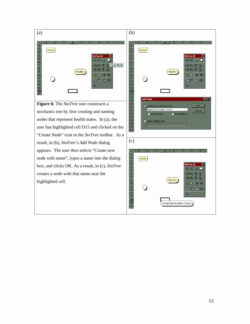
occupying one worksheet in the workbook. The user creates a node representing a health

state by selecting a worksheet cell near which the node should be placed and clicking on

the “Create Node” icon on the StoTree toolbar. Figure 6 illustrates this process. The user

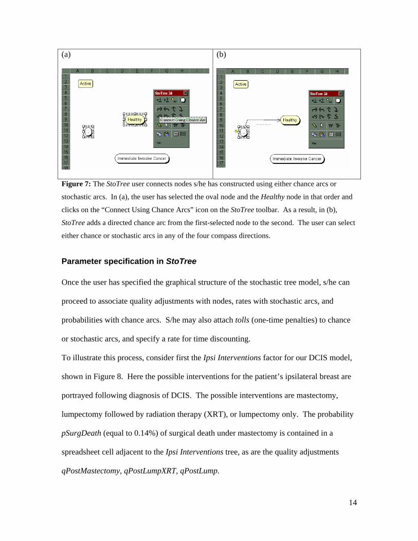
may connect any two created nodes with a chance or stochastic arc by clicking the

appropriate icon on the StoTree toolbar, as is described in Figure 7. StoTree also allows

the user to create decision nodes, terminal (death) nodes, and phantom nodes. The user

may also drag nodes to reposition them as desired, and then click on the Redraw icon on

the StoTree toolbar to have StoTree redraw all connecting arcs to match the new node

positions.

13

(a) (b)

Figure 6: The StoTree user constructs a

stochastic tree by first creating and naming

nodes that represent health states. In (a), the

user has highlighted cell D15 and clicked on the

“Create Node” icon in the StoTree toolbar. As a

result, in (b), StoTree’s Add Node dialog

appears. The user then selects “Create new

node with name”, types a name into the dialog

box, and clicks OK. As a result, in (c), StoTree

creates a node with that name near the

highlighted cell.

(c)

14

(a) (b)

Figure 7: The StoTree user connects nodes s/he has constructed using either chance arcs or

stochastic arcs. In (a), the user has selected the oval node and the Healthy node in that order and

clicks on the “Connect Using Chance Arcs” icon on the StoTree toolbar. As a result, in (b),

StoTree adds a directed chance arc from the first-selected node to the second. The user can select

either chance or stochastic arcs in any of the four compass directions.

Parameter specification in StoTree

Once the user has specified the graphical structure of the stochastic tree model, s/he can

proceed to associate quality adjustments with nodes, rates with stochastic arcs, and

probabilities with chance arcs. S/he may also attach tolls (one-time penalties) to chance

or stochastic arcs, and specify a rate for time discounting.

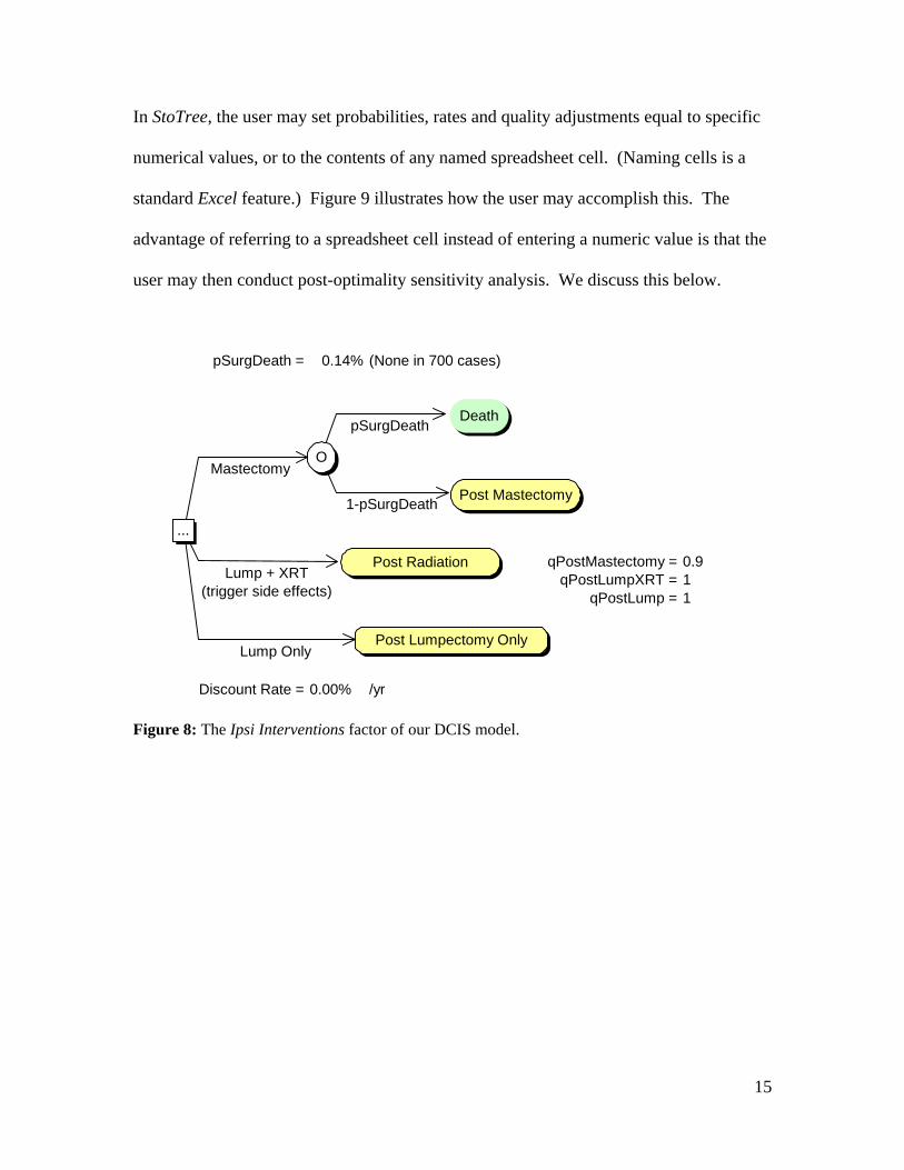
To illustrate this process, consider first the Ipsi Interventions factor for our DCIS model,

shown in Figure 8. Here the possible interventions for the patient’s ipsilateral breast are

portrayed following diagnosis of DCIS. The possible interventions are mastectomy,

lumpectomy followed by radiation therapy (XRT), or lumpectomy only. The probability

pSurgDeath (equal to 0.14%) of surgical death under mastectomy is contained in a

spreadsheet cell adjacent to the Ipsi Interventions tree, as are the quality adjustments

qPostMastectomy, qPostLumpXRT, qPostLump.

15

In StoTree, the user may set probabilities, rates and quality adjustments equal to specific

numerical values, or to the contents of any named spreadsheet cell. (Naming cells is a

standard Excel feature.) Figure 9 illustrates how the user may accomplish this. The

advantage of referring to a spreadsheet cell instead of entering a numeric value is that the

user may then conduct post-optimality sensitivity analysis. We discuss this below.

pSurgDeath = 0.14% (None in 700 cases)

35.863

35.9146

36.365

qPostMastectomy = 0.9qPostLumpXRT = 1

qPostLump = 134.751

Discount Rate = 0.00% /yr

Lump Only

Mastectomy

Lump + XRT (trigger side effects)

1-pSurgDeath

pSurgDeath

...

Post Radiation

Post Lumpectomy Only

Death

O

Post Mastectomy

Figure 8: The Ipsi Interventions factor of our DCIS model.

16

Figure 9: In StoTree, Probabilities and rates can be made to depend on named cells in the

spreadsheet. Here the probability on the highlighted arc from node O to Death is set equal to the

contents of the cell named pSurgDeath, which currently contains the value 0.14%. Similar

dependencies can be set up for quality adjustments. For instance, the quality adjustment for the

node Post Mastectomy has been set equal to the contents of the cell named qPostMastectomy,

whose value is currently 0.9.

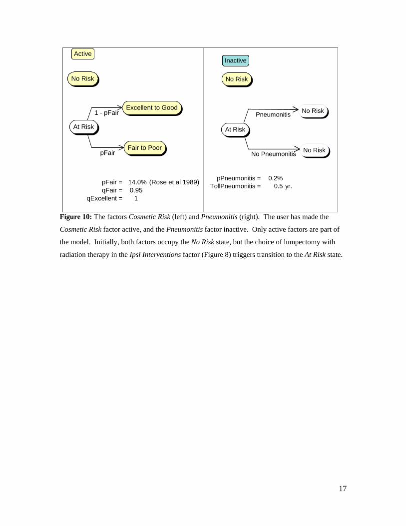
In the Ipsi Interventions factor, the choice of lumpectomy followed by radiation therapy

(Lump + XRT) has an associated risk of side effects. These side effects are depicted in

Figure 10, and include cosmetic effects such as breast shrinkage and toughening, as well

as pneumonitis. To instruct StoTree that the choice Lump + XRT triggers the risk of side

effects, the user selects the arc labeled Lump + XRT, clicks on the trigger icon on the

StoTree toolbar, and enters the desired trigger, as described in Figure 11.

17

36.62

34.79

pFair = 14.0% (Rose et al 1989)qFair = 0.95

qExcellent = 1

pFair

1 - pFair

Active

No Risk

At Risk

Excellent to Good

Fair to Poor

pPneumonitis = 0.2%TollPneumonitis = 0.5 yr.

No Pneumonitis

Pneumonitis

Inactive

No Risk

At Risk

No Risk

No Risk

Figure 10: The factors Cosmetic Risk (left) and Pneumonitis (right). The user has made the

Cosmetic Risk factor active, and the Pneumonitis factor inactive. Only active factors are part of

the model. Initially, both factors occupy the No Risk state, but the choice of lumpectomy with

radiation therapy in the Ipsi Interventions factor (Figure 8) triggers transition to the At Risk state.

18

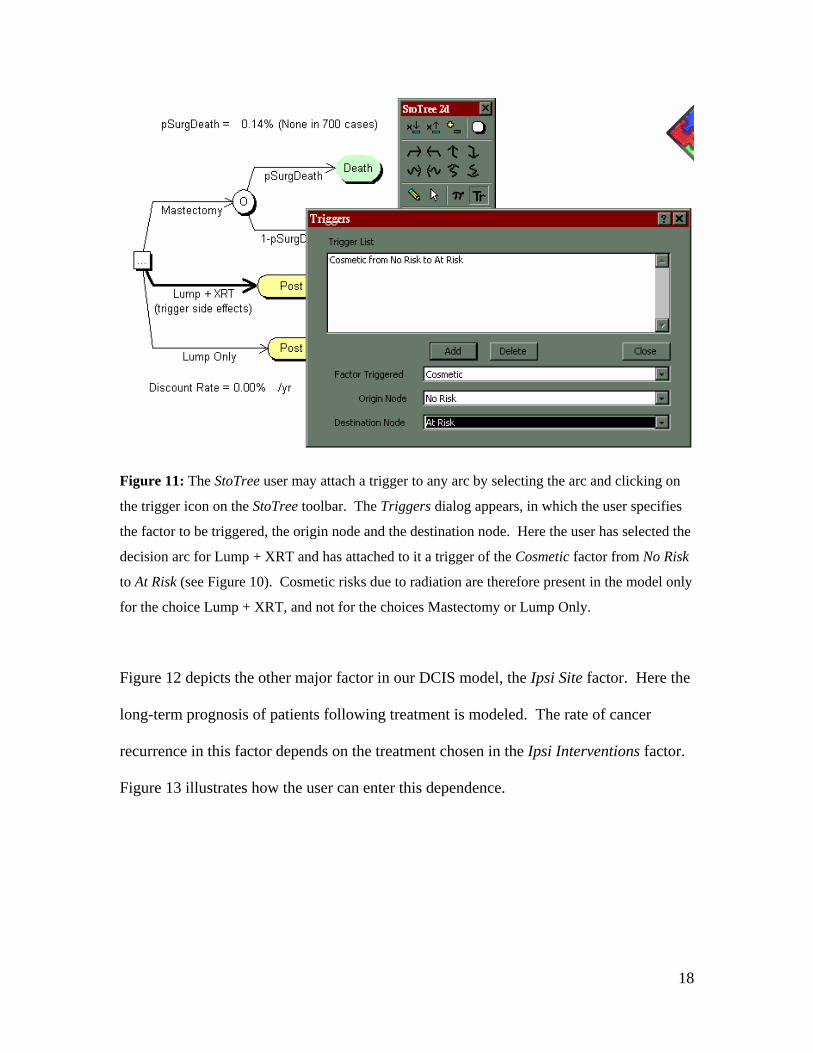
Figure 11: The StoTree user may attach a trigger to any arc by selecting the arc and clicking on

the trigger icon on the StoTree toolbar. The Triggers dialog appears, in which the user specifies

the factor to be triggered, the origin node and the destination node. Here the user has selected the

decision arc for Lump + XRT and has attached to it a trigger of the Cosmetic factor from No Risk

to At Risk (see Figure 10). Cosmetic risks due to radiation are therefore present in the model only

for the choice Lump + XRT, and not for the choices Mastectomy or Lump Only.

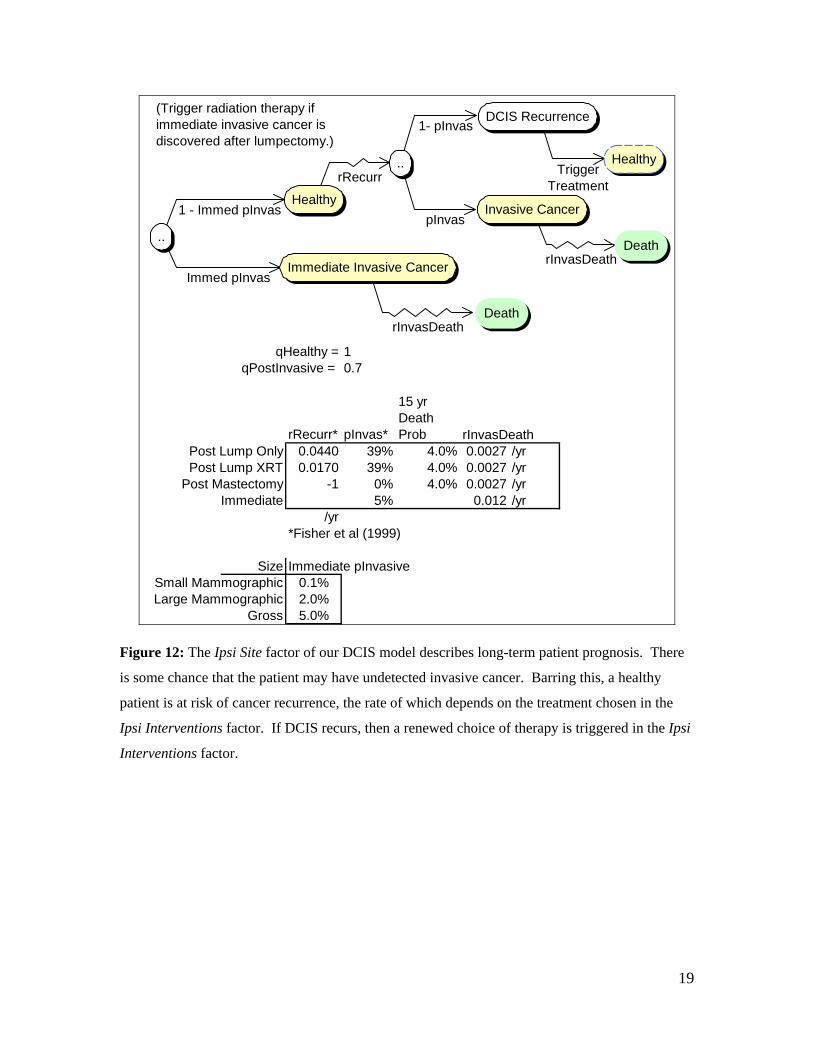
Figure 12 depicts the other major factor in our DCIS model, the Ipsi Site factor. Here the

long-term prognosis of patients following treatment is modeled. The rate of cancer

recurrence in this factor depends on the treatment chosen in the Ipsi Interventions factor.

Figure 13 illustrates how the user can enter this dependence.

19

35.5743525.871

19.23592

qHealthy = 1qPostInvasive = 0.7

rRecurr* pInvas*

15 yr Death Prob rInvasDeath

Post Lump Only 0.0440 39% 4.0% 0.0027 /yrPost Lump XRT 0.0170 39% 4.0% 0.0027 /yr

Post Mastectomy -1 0% 4.0% 0.0027 /yrImmediate 5% 0.012 /yr

/yr*Fisher et al (1999)

Size Immediate pInvasiveSmall Mammographic 0.1%Large Mammographic 2.0%

Gross 5.0%

Trigger Treatment

rInvasDeath

pInvas

1- pInvas

rRecurr

rInvasDeath

Immed pInvas

1 - Immed pInvasHealthy

DCIS Recurrence

Invasive Cancer

Death..

Immediate Invasive Cancer

Death

..

(Trigger radiation therapy if immediate invasive cancer is discovered after lumpectomy.)

Healthy

Figure 12: The Ipsi Site factor of our DCIS model describes long-term patient prognosis. There

is some chance that the patient may have undetected invasive cancer. Barring this, a healthy

patient is at risk of cancer recurrence, the rate of which depends on the treatment chosen in the

Ipsi Interventions factor. If DCIS recurs, then a renewed choice of therapy is triggered in the Ipsi

Interventions factor.

20

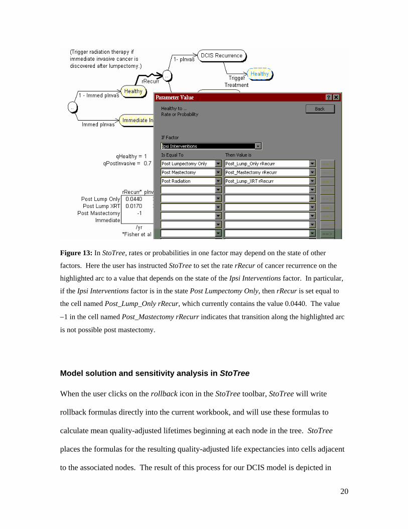
Figure 13: In StoTree, rates or probabilities in one factor may depend on the state of other

factors. Here the user has instructed StoTree to set the rate rRecur of cancer recurrence on the

highlighted arc to a value that depends on the state of the Ipsi Interventions factor. In particular,

if the Ipsi Interventions factor is in the state Post Lumpectomy Only, then rRecur is set equal to

the cell named Post_Lump_Only rRecur, which currently contains the value 0.0440. The value

−1 in the cell named Post_Mastectomy rRecurr indicates that transition along the highlighted arc

is not possible post mastectomy.

Model solution and sensitivity analysis in StoTree

When the user clicks on the rollback icon in the StoTree toolbar, StoTree will write

rollback formulas directly into the current workbook, and will use these formulas to

calculate mean quality-adjusted lifetimes beginning at each node in the tree. StoTree

places the formulas for the resulting quality-adjusted life expectancies into cells adjacent

to the associated nodes. The result of this process for our DCIS model is depicted in

21

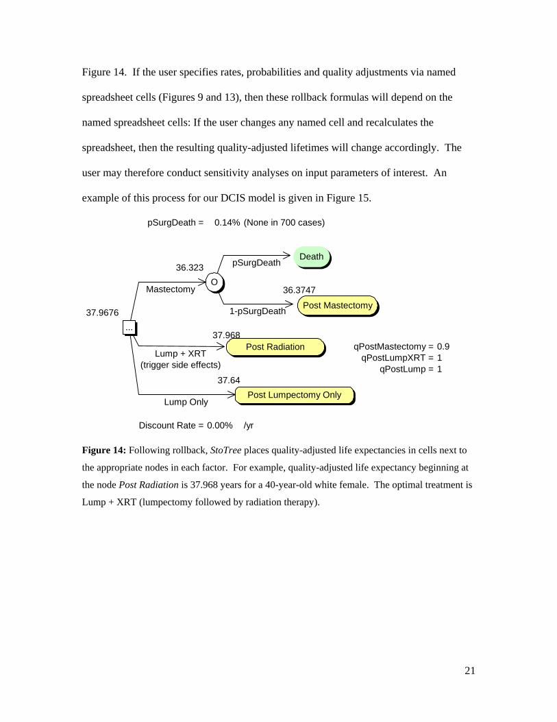
Figure 14. If the user specifies rates, probabilities and quality adjustments via named

spreadsheet cells (Figures 9 and 13), then these rollback formulas will depend on the

named spreadsheet cells: If the user changes any named cell and recalculates the

spreadsheet, then the resulting quality-adjusted lifetimes will change accordingly. The

user may therefore conduct sensitivity analyses on input parameters of interest. An

example of this process for our DCIS model is given in Figure 15.

pSurgDeath = 0.14% (None in 700 cases)

36.323

36.3747

37.9676

37.968qPostMastectomy = 0.9

qPostLumpXRT = 1qPostLump = 1

37.64

Discount Rate = 0.00% /yr

Lump Only

Mastectomy

Lump + XRT (trigger side effects)

1-pSurgDeath

pSurgDeath

...

Post Radiation

Post Lumpectomy Only

Death

O

Post Mastectomy

Figure 14: Following rollback, StoTree places quality-adjusted life expectancies in cells next to

the appropriate nodes in each factor. For example, quality-adjusted life expectancy beginning at

the node Post Radiation is 37.968 years for a 40-year-old white female. The optimal treatment is

Lump + XRT (lumpectomy followed by radiation therapy).

22

pSurgDeath = 0.14% (None in 700 cases)

40.359

40.4164

40.3588

38.683qPostMastectomy = 1

qPostLumpXRT = 1qPostLump = 1

37.991

Discount Rate = 0.00% /yr

Lump Only

Mastectomy

Lump + XRT (trigger side effects)

1-pSurgDeath

pSurgDeath

...

Post Radiation

Post Lumpectomy Only

Death

O

Post Mastectomy

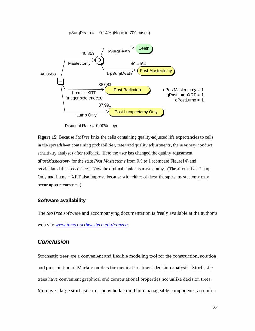
Figure 15: Because StoTree links the cells containing quality-adjusted life expectancies to cells

in the spreadsheet containing probabilities, rates and quality adjustments, the user may conduct

sensitivity analyses after rollback. Here the user has changed the quality adjustment

qPostMastectomy for the state Post Mastectomy from 0.9 to 1 (compare Figure14) and

recalculated the spreadsheet. Now the optimal choice is mastectomy. (The alternatives Lump

Only and Lump + XRT also improve because with either of these therapies, mastectomy may

occur upon recurrence.)

Software availability

The StoTree software and accompanying documentation is freely available at the author’s

web site www.iems.northwestern.edu/~hazen.

Conclusion

Stochastic trees are a convenient and flexible modeling tool for the construction, solution

and presentation of Markov models for medical treatment decision analysis. Stochastic

trees have convenient graphical and computational properties not unlike decision trees.

Moreover, large stochastic trees may be factored into manageable components, an option

23

of considerable value in model formulation and model presentation. The freely available

software StoTree implements these features using a graphical modeling interface within

the familiar spreadsheet environment. This environment allows easy substitution and

swapping of model components, and convenient sensitivity analysis capabilities.

References

JR Beck, JP Kassirer, SG Pauker (1982), “A Convenient Approximation of Life Expectancy (the “DEALE”): I. Validation of the method”, Am J Med 73, 883-888.

JR Beck and SG Pauker (1983), “The Markov Process in Medical Prognosis,” Medical Decision Making 3, 419−458.

G.B. Hazen (1992), "Stochastic Trees: A New Technique for Temporal Medical Decision Modeling," Medical Decision Making 12, 163-178.

G.B. Hazen (1993), "Factored Stochastic Trees: A Tool for Solving Complex Temporal Medical Decision Models," Medical Decision Making 13, 227-236.

GB Hazen, M Morrow, ER Venta, "Patient Values in the Treatment of Ductal Carcinoma in Situ", Society for Medical Decision Making Annual Meeting, Reno, Nevada, October 1999.

H. Hiramatsu, BA Bornstein, A Recht, SJ Schnitt, JK Baum, JL Connolly, RB Duda, AJ Guidi, CM Kaelin, B Silver, JR Harris, “Local Recurrence After Conservative Surgery and Radiation Therapy for Ductal Carcinoma in Situ”, Cancer J Sci Am 1995; 1:55-61.

JP Hollenberg (1984), “Markov Cycle Trees: A New Representation for Complex Markov Processes”, (abstr.), Medical Decision Making 4, 529.

DB Matchar and SG Pauker (1986), “Transient Ischemic Attacks in a Man with Coronary Artery Disease: Two Strategies Neck and Neck”, Medical Decision Making 6, 239-249.

MJ Silverstein, BF Cohen, ED Gierson, M Furmanski, P Gamagami, WJ Colburn, BS Lewinsky, JR Waisman, “Duct Carcinoma in situ: 227 Cases Without Microinvasion”, Eur J Cancer 28 (1992) 630-634.

FA Sonnenberg and JR Beck (1993), “Markov Models in Medical Decision Making: A Practical Guide”, Medical Decision Making 13, 322-338.