1

A Stochastic Approach for the Analysis of

Fault Trees with Priority AND Gates

Peican Zhu, Jie Han, Leibo Liu and Ming J. Zuo

Abstract—Dynamic fault tree (DFT) analysis has been used to account for the dynamic

behaviors such as the sequence-dependent, functional-dependent and priority relationships

among the failures of basic events. Various methodologies have been developed to analyze a

DFT; however, most methods require a complex analytical procedure or a significant

simulation time for an accurate analysis. In this paper, a stochastic computational

approach is proposed for an efficient analysis of the top event’s failure probability in a

DFT with priority AND (PAND) gates. A stochastic model is initially proposed for a two-

input PAND gate and a successive cascading model is then presented for a general

multiple-input PAND gate. A stochastic approach using the proposed models provides an

efficient analysis of a DFT compared to an accurate analysis or algebraic approach. The

accuracy of a stochastic analysis increases with the length of random binary bit streams in

stochastic computation. The use of non-Bernoulli sequences of random permutations of

fixed numbers of 1’s and 0’s as initial input events’ probabilities makes the stochastic

approach more efficient and more accurate than Monte Carlo simulation. Non-exponential

failure distributions and repeated events are readily handled by the stochastic approach.

The accuracy, efficiency and scalability of the stochastic approach are shown by several

case studies of DFT analysis.

2

Index Terms—Dynamic fault tree (DFT), reliability analysis, stochastic computation, non-

Bernoulli sequence, priority AND (PAND) gate, stochastic logic.

ACRONYM

FTA fault tree analysis

DFT dynamic fault tree

FDEP functional dependency gate

PAND priority AND gate

SEQ sequence enforcing gate

WSP warm spare gate

CSP cold spare gate

pdf probability density function

cdf cumulative density function

BDDs binary decision diagrams

SBDDs sequential binary decision diagrams

MC Monte Carlo

FPGA Field Programmable Gate Array

NOTATION

→ symbol for an inclusive precedence in a failure order

3

𝑡 mission time

𝐴, 𝐵, 𝐶, 𝐷,⋯ basic events

λ failure rate

𝐹𝑡(𝐴) failure time of basic event 𝐴

𝐹(𝑡𝑖) failure probability in the time interval [𝑡𝑖, 𝑡𝑖 + 𝛥𝑡]

𝑆(𝑡𝑖) binary sequence at 𝑡𝑖

𝐿 sequence length in the number of bits

I. INTRODUCTION

AULT tree analysis (FTA) was first proposed in 1962 for evaluating a system’s failure

probability - the probability that a system fails during a specified mission time [1]. Failures can

be disastrous for systems such as chemical plants, nuclear reactors, airplane and computer

systems, or costly for systems such as online sales or commercial servers. FTA has developed

rapidly and gained much attention in many applications, especially in the analysis of large

safety-critical systems [2-7].

However, dynamic behaviors, such as sequence-dependent, functionally dependent and priority

relationships, cannot be modeled properly by traditional FTA. To account for these dynamic

behaviors, dynamic fault tree (DFT) analysis has been proposed by incorporating additional

dynamic gates into FTA. Dynamic gates include the priority AND gate (PAND), the sequence

enforcing gate (SEQ), the standby or spare gates that include the warm spare gate (WSP) and

cold spare gate (CSP), and the functional dependency gate (FDEP) [8, 9]. The failure of a system

is determined by the states of basic events and the interactions among them. The interactions can

F

4

be derived from a system’s topology. A DFT relies on the interactions among static gates

(including AND, OR, and K-out-of-N voting gate) and dynamic gates (PAND, FDEP, SPARE,

and SEQ) [10]. Due to their operational characteristics, the dynamic gates are divided into two

categories: (1) PAND and FDEP, which are referred to as priority dynamic gates; (2) WSP and

SEQ, whose operations are dependent on the duration of failure events [11]. For systems with a

perfect fault coverage, FDEP has been modeled as an OR gate [12 - 15]. In a redundant system

with an imperfect fault coverage, however, uncovered or undetected faults can propagate and

may have a global effect to system failure [16]. In this case, the OR-gate model is not applicable

and a combinatorial method has been proposed for an efficient reliability analysis of systems

with FDEP gates [16]. As a first study, this paper is focused on priority dynamic gates and, in

particular, the PAND gate.

Various methodologies using Markov [2] and Bayesian [17] models have been proposed

for evaluating the dependability of a fault tree. Due to the inevitable state-space explosion

problem, however, these approaches incur a large complexity for the analysis of complex

systems. Moreover, the evaluation of a large DFT using a state-space based method becomes

difficult when a basic event’s failure behavior is not exponentially distributed.

In [2], an Inclusion/Exclusion method is proposed for an exact analysis of a DFT that

contains PAND gates and repeated events. However, this method is limited to the analysis of

systems with exponentially distributed failure events; in addition, detailed information on the

minimal cut set is usually required in advance. In [7] an integral-based analysis is proposed for

handling any probability distribution; however an analytical expression is generally difficult to

derive as a function of the basic events’ failure distributions. Several approaches have been

developed to simplify the process of deriving an exact analytical expression. These include those

5

using binary decision diagrams (BDDs) [18], sequential binary decision diagrams (SBDDs) [19,

20] and an algebraic analysis [11, 21]. In particular, the SBDD approach has been applied to the

analysis of PAND gate [22]. Monte Carlo (MC) simulation [23] has been widely used to evaluate

complex DFTs; however, a long run time and a large sample size are needed to meet an accuracy

requirement, because of the slow convergence typically encountered in an MC simulation.

Generally, it is challenging to efficiently and accurately evaluate the reliability of a DFT.

A stochastic approach has been proposed in [15] for an efficient evaluation of a system’s

reliability. In particular, the serial and parallel implementations of stochastic computation are

considered and a speedup in analysis is obtained by a parallel implementation in FPGAs. In [15],

the PAND gate is modeled as a three-input AND gate and a sequential event is considered as a

basic event. In a general case, however, the input of a PAND gate is not limited to a basic event.

In this paper, a new stochastic approach is presented for an efficient analysis of fault trees

with PAND gates. Initially, a stochastic computational model is proposed for the PAND gate; in

this model, the output failure probability is obtained as a function of the basic inputs’ failure

probabilities. Thus, this model is applicable in the general case of a multiple-input PAND gate

through a cascaded PAND model. Subsequently, non-Bernoulli sequences of random

permutations of fixed numbers of 1’s and 0’s are used to represent initial event probabilities for

an efficient implementation of stochastic computation. It has been shown that the use of the non-

Bernoulli sequences as initial inputs provides a more efficient and accurate evaluation than using

Bernoulli sequences [24, 25]. This paper shows that the non-Bernoulli sequences significantly

improves the efficiency of a stochastic FTA. Hence, the advantage of the stochastic approach is

not limited to those due to parallelization or a specific hardware implementation. Furthermore,

repeated events, as frequently encountered in a general DFT, are inherently modeled by the

6

stochastic sequences that preserve signal correlation. Finally, the stochastic approach is general

because it is applicable to any failure distribution by encoding failure probabilities into stochastic

non-Bernoulli sequences.

The remainder of the paper is organized as follows. Section II reviews the definitions of

PAND. Section III presents some hypotheses considered in this paper. The stochastic approach

and the proposed model for the PAND gate are described in Section IV. In Section V, the

accuracy and efficiency of the proposed approach are shown by the simulation results of several

examples. Finally, Section VI concludes the paper.

II. REVIEW OF PAND GATE

A PAND gate is a special type of AND gate, for which an input indicates the firing of a

basic event that occurs in a predetermined order and the output indicates whether a failure occurs

[5, 26]. Without the loss of generality, the predefined order is assumed to be from left to right in

this paper unless otherwise noted. The operational principles of a two-input PAND gate, as well

as its symbols, are shown in Fig. 1 for an inclusive condition [11]. By an inclusive condition, if

the two inputs of the PAND gate fail simultaneously, the output fails at the same time as the

inputs.

PAND

A B

OUT

AND

A B

OUT

A Before B

(a)

7

Case 1

10

10

OUT

B

10A

t Case 2 t Case 3t

10

10

10

10

10

10

OUT

B

A

OUT

B

A

(b)

Fig. 1 (a) Symbols for a two-input PAND gate [5, 26]; (b) The expected behaviour of the two-input PAND gate for

an inclusive condition (adapted from [11]); 1 and 0 indicate faulty and fault-free events respectively.

As shown in Fig. 1, the output of the PAND gate is 1 (i.e., it fails) when the basic event 𝐴

fails before 𝐵 or 𝐴 and 𝐵 fail at the same time; otherwise, the output of the PAND gate is 0, i.e.,

fault free. Let 𝐹𝑡(𝐴) and 𝐹𝑡(𝐵) be the failure time of basic events 𝐴 and 𝐵 respectively; the

failure time of the PAND gate’s output, 𝐹𝑡(𝑂𝑈𝑇), is given by:

𝐹𝑡(𝑂𝑈𝑇) = {

𝐹𝑡(𝐵), 𝑖𝑓 𝐹𝑡(𝐴) < 𝐹𝑡(𝐵)

𝐹𝑡(𝐴) 𝑜𝑟 𝐹𝑡(𝐵), 𝑖𝑓 𝐹𝑡(𝐴) = 𝐹𝑡(𝐵)

∞, 𝑖𝑓 𝐹𝑡(𝐴) > 𝐹𝑡(𝐵)

(1)

III. HYPOTHESES

Some hypotheses of the paper are as follows:

The quantization level of a basic event is denoted by a binary variable 𝑥, 𝑥 ∈ {0,1}, with 0

indicating no fault;

All basic events are fault-free at the beginning of the mission time;

The basic events are non-repairable [5]. This means that if a basic event fails, the variable

that indicates the status of the basic event, takes 1. Let 𝐹𝑡(𝑎) be the failure time of a basic

8

event 𝑎; the status variable of 𝑎 is 1 for time 𝑡 > 𝐹𝑡(𝑎) and 0 otherwise. A generic timing

diagram for a non-repairable basic event 𝑎 is shown in Fig. 2.

The probability density function (pdf) and cumulative density function (cdf) of an

exponential distribution are given by:

𝑓(𝑡) = 𝜆 𝑒−𝜆𝑡, (2)

and

𝐹(𝑡) = ∫ 𝑓(𝑡)𝑡

0𝑑𝑡 = 1 − 𝑒−𝜆𝑡, (3)

where 𝑡 is the specified mission time and 𝜆 is the (constant) failure rate of a basic event for

an exponential distribution.

The failure probability of a basic event in a selected time interval [𝑡𝑖 , 𝑡𝑖 + 𝛥𝑡] is considered

constant at the value in the beginning of the time interval, i.e., the failure probability is given

by 𝑝 = 𝐹(𝑡𝑖) for any time in this time interval. For simplicity, the time interval [𝑡𝑖, 𝑡𝑖 + 𝛥𝑡]

is referred to as time i in this paper.

tFt(a)

a 1

0

Fig. 2 A timing diagram for a non-repairable basic event 𝑎 [5, 11]. A value of 0 indicates no fault while 1 means the

event has failed; 𝐹𝑡(𝑎) is the failure time of the basic event 𝑎.

IV. STOCHASTIC PAND MODEL

A. Stochastic computational models

Stochastic computation was introduced in the 1960s for reliable circuit design [27]. In

9

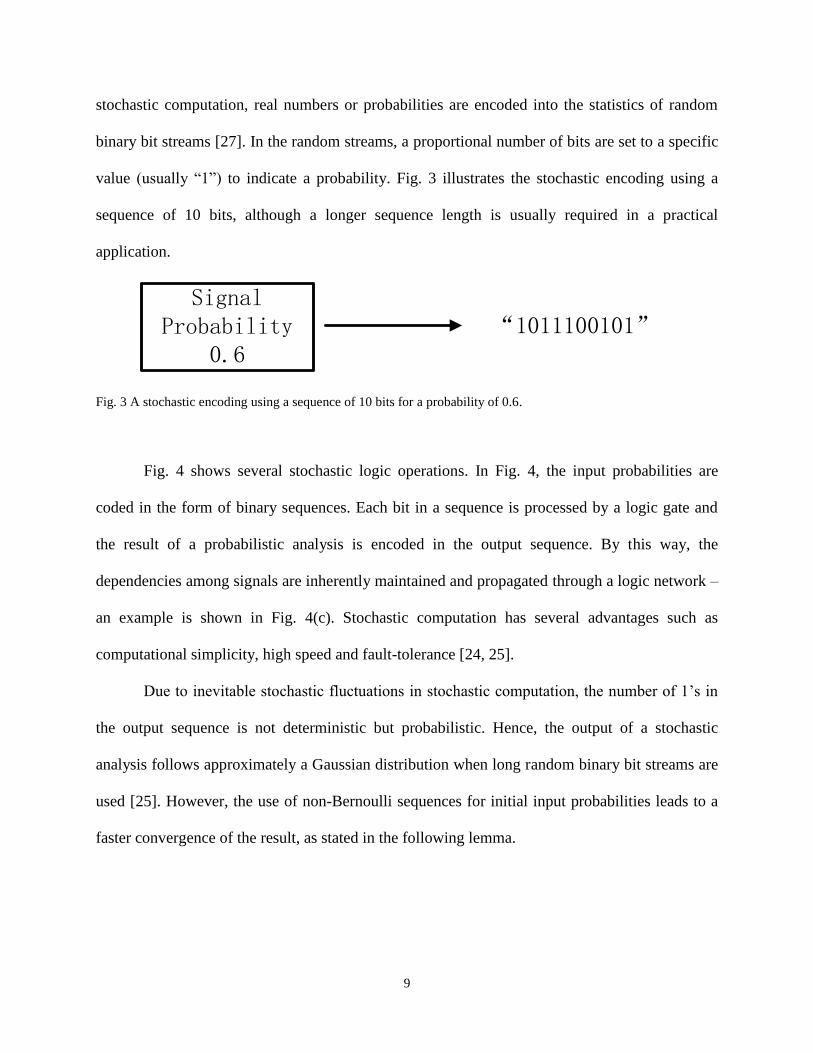
stochastic computation, real numbers or probabilities are encoded into the statistics of random

binary bit streams [27]. In the random streams, a proportional number of bits are set to a specific

value (usually “1”) to indicate a probability. Fig. 3 illustrates the stochastic encoding using a

sequence of 10 bits, although a longer sequence length is usually required in a practical

application.

Signal Probability

0.6“1011100101”

Fig. 3 A stochastic encoding using a sequence of 10 bits for a probability of 0.6.

Fig. 4 shows several stochastic logic operations. In Fig. 4, the input probabilities are

coded in the form of binary sequences. Each bit in a sequence is processed by a logic gate and

the result of a probabilistic analysis is encoded in the output sequence. By this way, the

dependencies among signals are inherently maintained and propagated through a logic network –

an example is shown in Fig. 4(c). Stochastic computation has several advantages such as

computational simplicity, high speed and fault-tolerance [24, 25].

Due to inevitable stochastic fluctuations in stochastic computation, the number of 1’s in

the output sequence is not deterministic but probabilistic. Hence, the output of a stochastic

analysis follows approximately a Gaussian distribution when long random binary bit streams are

used [25]. However, the use of non-Bernoulli sequences for initial input probabilities leads to a

faster convergence of the result, as stated in the following lemma.

10

……1110……

……0110……

……0110……

9.01 P

9.02 P

0111111101

8.02 P

9.0P

11111111011110000101

5.01 P

……1110……9.021 PP

……1110……

(b)

(c) (d)

81.021 PPP

9.0)1()1(1 21 PPP9.021 PPP

9.0P

81.0P

……1110…… ……0001……

4.01 P 6.0P

6.01 1 PP

(a)

Fig. 4 Stochastic logic: (a) An inverter with a random binary bit sequence as the input; (b) An AND gate with

independent inputs; (c) An AND gate with totally correlated inputs; (d) An OR gate with independent inputs.

Lemma 1. [Theorem 1 in [25]] Compared to the case when Bernoulli sequences are used

to represent initial input probabilities, the use of large non-Bernoulli sequences as random

permutations of fixed numbers of 1’s and 0’s results in an output sequence with the same mean

number of 1’s and a smaller variance for an AND gate with independent inputs.

Lemma 1 leads to the conclusion that, to meet a specific accuracy requirement, a smaller

sequence length is required by using the non-Bernoulli sequences compared to the use of

Bernoulli sequences for encoding initial input probabilities of an AND gate [25].

It is trivial to show that Lemma 1 is also applicable to an inverter, thus any logic network

(as combinations of inverters and AND gates) can be more efficiently and accurately evaluated

by using the non-Bernoulli sequences as initial input probabilities. When the inputs of a gate are

correlated, the output is also determined by the correlation between the input signals. However,

signal correlation (usually caused by the reconvergence of signals) is handled efficiently in

11

stochastic computation. This is particularly a favorable property for handling the repeated input

events in a complex DFT.

B. A two-input PAND gate model

Let 𝐴𝑖−1 and 𝐵𝑖−1 indicate the states of basic events 𝐴 and 𝐵 at time 𝑖 − 1, and 𝐴𝑖 and 𝐵𝑖

for the states at time 𝑖. If both 𝐴 and 𝐵 fail at time 𝑖, i.e., 𝐴𝑖−1𝐵𝑖−1 = 00 and 𝐴𝑖𝐵𝑖 = 11, the

failure time of the basic events 𝐴 and 𝐵 is given by:

𝐹𝑡(𝐴) = 𝐹𝑡(𝐵) = 𝑖 ∙ ∆𝑡. (4)

Then, the failure time of the PAND gate’s output is given by 𝐹𝑡(𝑂𝑈𝑇) = 𝐹𝑡(𝐴) =

𝐹𝑡(𝐵) = 𝑖 ∙ ∆𝑡, due to the model considered in Case 2 in Fig. 1(b).

If 𝐴𝑖−1𝐵𝑖−1 = 10 and 𝐴𝑖𝐵𝑖 = 11 at time 𝑖 − 1 and 𝑖 , the basic event 𝐵 fails at time 𝑖

while 𝐴 fails before time 𝑖. The failure time of the basic event 𝐵 is then:

𝐹𝑡(𝐵) = 𝑖 ∙ ∆𝑡. (5)

The relationship between the failure times of the basic events 𝐴 and 𝐵 is given by:

𝐹𝑡(𝐴) < 𝐹𝑡(𝐵). (6)

Thus, 𝐹𝑡(𝑂𝑈𝑇) = 𝐹𝑡(𝐵), due to (1) and the model considered in Case 1 in Fig. 1(b).

For the other possible scenario, i.e., the basic event 𝐴 fails after 𝐵, the top event of the

PAND gate would not fail, i.e., with a failure time of infinity, due to the model considered in

Case 3 in Fig. 1(b).

Since the basic events are non-repairable, the state of the two-input PAND gate’s output

event is affected by the gate’s output at the previous time, hence the output of the PAND gate at

time i, 𝑂𝑈𝑇𝑖, is determined by:

(1) The current states of the input basic events 𝐴 and 𝐵 at time 𝑖, 𝐴𝑖 and 𝐵𝑖;

(2) The inverted state of basic event 𝐵 at time 𝑖 − 1, 𝑁𝑂𝑇(𝐵𝑖−1);

12

(3) The output of the PAND gate at time 𝑖 − 1, 𝑂𝑈𝑇𝑖−1.

Hence, the output of the PAND gate at time 𝑖 is given by

𝑂𝑈𝑇𝑖 = 𝑂𝑈𝑇𝑖−1 + 𝐴𝑖 ∙ 𝐵𝑖 ∙ 𝑁𝑂𝑇(𝐵𝑖−1) (7)

A stochastic logic model can be constructed to determine the failure of the two-input

PAND gate, as shown in Fig. 5.

iOUT

1iOUT

iA

iB

1iB iDiE

iA

iB

1iB

iE

iDiF

)(a

)( b

Fig. 5 (a) A stochastic logic model for a two-input PAND gate and (b) the decomposition of the three-input AND

gate in (a) into two-input AND gates. 𝐴𝑖−1 and 𝐵𝑖−1 indicate the states of basic events 𝐴 and 𝐵 at time 𝑖 − 1; 𝐴𝑖 and

𝐵𝑖 are the states at time 𝑖; 𝑂𝑈𝑇𝑖 and 𝑂𝑈𝑇𝑖−1 are the states of the gate’s output event at time 𝑖 and 𝑖 − 1

respectively.

As per the hypothesis in section III, all basic events are fault free at the beginning of the

mission time; thus, the input signals of the model in Fig. 5 are zeros. In Fig. 5(a), if the basic

event 𝐴 fails before time 𝑖, 𝐸𝑖 = 1 if 𝐵𝑖−1 = 0 and 𝐵𝑖 = 1. Then at time 𝑖, 𝑂𝑈𝑇𝑖 = 1. However,

if 𝑂𝑈𝑇𝑖−1 = 1, which indicates that 𝐴 fails before 𝐵 or both events fail simultaneously at time

𝑖 − 1, then 𝐵𝑖−1 = 1 and 𝐸𝑖 = 0 . Since 𝑂𝑈𝑇𝑖−1 and 𝐸𝑖 cannot be 1 at the same time, either

𝑂𝑈𝑇𝑖−1 = 1 or 𝐸𝑖 = 1 results in 𝑂𝑈𝑇𝑖 = 1. Otherwise, the state of the top event remains zero.

13

From this analysis, it can be seen that the stochastic PAND model in Fig. 5 computes (7), thus it

accurately implements the function of the PAND gate.

C. Model validation

To validate the proposed stochastic PAND model, the discretization of a continuous

probability distribution and the generation of stochastic non-Bernoulli sequences are introduced

next, followed by a theoretical proof.

1) Discretization

Assume that the mission time 𝑡 is divided into M equal time intervals, i.e., 𝛥𝑡 = 𝑡/𝑀.

Due to the nature of discretization, a failure probability is estimated more precisely at time t with

a larger 𝑀. However, a longer run time is required as more stochastic sequences need to be

generated. Hence, 𝑀 is determined by a tradeoff between accuracy and efficiency. With a

reasonable 𝑀 , the discretization provides a relatively accurate estimation of the continuous

failure probability of a basic event.

2) Generation of non-Bernoulli sequences

Assume that the failure probabilities for the two adjacent time intervals, [𝑡𝑖 − 𝛥𝑡, 𝑡𝑖] and

[𝑡𝑖, 𝑡𝑖 + 𝛥𝑡], are given by 𝐹(𝑡𝑖 − 𝛥𝑡) and 𝐹(𝑡𝑖) respectively. If non-Bernoulli sequences of 𝐿 bits,

as random permutation of fixed number of 0’s and 1’s, are used, the number of 1’s in these

sequences for the two probabilities are given by:

{𝑁(𝑡𝑖 − 𝛥𝑡) = 𝐿 ∙ 𝐹(𝑡𝑖 − 𝛥𝑡),

𝑁(𝑡𝑖) = 𝐿 ∙ 𝐹(𝑡𝑖). (8)

The difference of the number of 1’s is then:

𝛥𝑁 = 𝑁(𝑡𝑖) − 𝑁(𝑡𝑖 − 𝛥𝑡) = 𝐿 ∙ [𝐹(𝑡𝑖) − 𝐹(𝑡𝑖 − 𝛥𝑡)]. (9)

Further assume that the non-Bernoulli sequence for the probability in [𝑡𝑖 − 𝛥𝑡, 𝑡𝑖] is

14

given by 𝑆(𝑡𝑖 − 𝛥𝑡), then the sequence 𝑆(𝑡𝑖) for the probability in [𝑡𝑖 , 𝑡𝑖 + 𝛥𝑡] can be obtained

by randomly assigning 𝛥𝑁 1’s to replace the 0’s in 𝑆(𝑡𝑖 − 𝛥𝑡)𝑗. Since the 1’s in 𝑆(𝑡𝑖 − 𝛥𝑡) are a

subset of those in 𝑆(𝑡𝑖), we obtain:

𝑆(𝑡𝑖 − 𝛥𝑡) 𝐴𝑁𝐷 𝑆(𝑡𝑖) = 𝑆(𝑡𝑖 − 𝛥𝑡). (10)

3) Stochastic model validation

Theorem 1: Compared to an accurate analysis method, a stochastic simulation of the

two-input PAND gate model in Fig. 5, using large non-Bernoulli sequences of random

permutations of fixed numbers of 1’s and 0’s as initial input probabilities, produces the same

increment in the failure probabilities of two adjacent time intervals when 𝜆𝛥𝑡 → 0.

Proof: Assume that the failure probabilities of the PAND gate at time i and i-1 are given

by 𝐹((𝐴 → 𝐵)𝑖) and 𝐹((𝐴 → 𝐵)𝑖−1), respectively; we show that the failure probability of 𝐸𝑖 in

the stochastic model in Fig. 5 is the same as the increment in the output failure probability of the

PAND gate from time i-1 to i, i.e., 𝐹(𝐸𝑖) = 𝐹((𝐴 → 𝐵)𝑖) − 𝐹((𝐴 → 𝐵)𝑖−1).

Given the basic events 𝐴 and 𝐵 with the probability density functions (pdfs) 𝑓𝐴(𝑡)and

𝑓𝐵(𝑡) respectively, the failure probability for the two-input PAND gate’s output 𝑂𝑈𝑇 (when both

𝐴 and 𝐵 fail or 𝐴 fails before 𝐵, i.e., 𝐴 → 𝐵), is given by:

𝐹(𝐴 → 𝐵) = ∫ ∫ 𝑓𝐵(𝑡2)𝑓𝐴(𝑡1)𝑑𝑡2𝑡

𝑡1

𝑡

0𝑑𝑡1, (11)

For an exponential distribution, (11) becomes:

𝐹(𝐴 → 𝐵) = ∫ ∫ 𝜆𝐵𝑒−𝜆𝐵𝑡2𝜆𝐴𝑒−𝜆𝐴𝑡1𝑑𝑡2𝑡

𝑡1

𝑡

0𝑑𝑡1 , (12)

which leads to the failure probability of the sequential event 𝐴 → 𝐵 as:

𝐹(𝐴 → 𝐵) =𝜆𝐴

(𝜆𝐴+𝜆𝐵)(1 − 𝑒−(𝜆𝐴+𝜆𝐵)𝑡) − 𝑒−𝜆𝐵𝑡(1 − 𝑒−𝜆𝐴𝑡). (13)

(13) can be obtained by using an analytical approach [7] or a probabilistic algebraic analysis

15

[11].

By discretization, the failure probabilities of the sequential event 𝐴 → 𝐵 at time 𝑖 and 𝑖 −

1 are given by:

𝐹((𝐴 → 𝐵)𝑖) =𝜆𝐴

(𝜆𝐴+𝜆𝐵)(1 − 𝑒−(𝜆𝐴+𝜆𝐵)∙𝑖∙𝛥𝑡) − 𝑒−𝜆𝐵∙𝑖∙𝛥𝑡(1 − 𝑒−𝜆𝐴∙𝑖∙𝛥𝑡), (14)

and

𝐹((𝐴 → 𝐵)𝑖−1) =𝜆𝐴

(𝜆𝐴+𝜆𝐵)(1 − 𝑒−(𝜆𝐴+𝜆𝐵)∙(𝑖−1)∙𝛥𝑡) − 𝑒−𝜆𝐵∙(𝑖−1)∙𝛥𝑡 + 𝑒−(𝜆𝐴+𝜆𝐵)∙(𝑖−1)∙𝛥𝑡, (15)

respectively. (14) can also be written as:

𝐹((𝐴 → 𝐵)𝑖) =𝜆𝐴

(𝜆𝐴+𝜆𝐵)(1 − 𝑒−(𝜆𝐴+𝜆𝐵)∙(𝑖−1)∙𝛥𝑡 ∙ 𝑒−(𝜆𝐴+𝜆𝐵)∙𝛥𝑡) − 𝑒−𝜆𝐵∙(𝑖−1)∙𝛥𝑡 ∙ 𝑒−𝜆𝐵∙𝛥𝑡 +

𝑒−(𝜆𝐴+𝜆𝐵)∙(𝑖−1)∙𝛥𝑡 ∙ 𝑒−(𝜆𝐴+𝜆𝐵)∙𝛥𝑡. (16)

Since 𝑂((𝜆 ∙ ∆𝑡)𝑖) for any 𝑖 ≥ 2 is negligible when 𝜆𝛥𝑡 → 0, applying a Taylor series

expansion on (16) leads to:

𝐹((𝐴 → 𝐵)𝑖) = [𝜆𝐴

(𝜆𝐴+𝜆𝐵)(1 − 𝑒−(𝜆𝐴+𝜆𝐵)∙(𝑖−1)∙𝛥𝑡) − 𝑒−𝜆𝐵∙(𝑖−1)∙𝛥𝑡 + 𝑒−𝜆𝐵∙(𝑖−1)∙𝛥𝑡 ∙ 𝜆𝐵 ∙ 𝛥𝑡 +

𝑒−(𝜆𝐴+𝜆𝐵)∙(𝑖−1)∙𝛥𝑡 − 𝑒−(𝜆𝐴+𝜆𝐵)∙(𝑖−1)∙𝛥𝑡 ∙ 𝜆𝐵 ∙ 𝛥𝑡]. (17)

From (15) and (17), the probability increment for two adjacent times is obtained as:

𝐹(𝑂𝑈𝑇𝑖) − 𝐹(𝑂𝑈𝑇𝑖−1) = 𝐹((𝐴 → 𝐵)𝑖) − 𝐹((𝐴 → 𝐵)𝑖−1)

= 𝜆𝐵 ∙ 𝛥𝑡 ∙ 𝑒−𝜆𝐵∙(𝑖−1)∙𝛥𝑡 ∙ (1 − 𝑒−(𝜆𝐴)∙(𝑖−1)∙𝛥𝑡). (18)

Next, the stochastic analysis of the increased probability 𝐸𝑖 between two adjacent times is

pursued. Let 𝐹𝑐(∙) and 𝐹𝑑(∙) indicate the cumulative density functions (cdfs) for the continuous

and discretized distributions respectively. By applying the discretization process to the

exponential distributions of the basic events (i.e., 𝐴 and 𝐵), we have:

{𝐹𝑐(𝐴) = ∫ 𝑓𝐴(𝑡)

𝑡

0𝑑𝑡 = 1 − 𝑒−𝜆𝐴∙𝑡,

𝐹𝑑(𝐴) = 1 − 𝑒−𝜆𝐴∙𝑀∙∆𝑡, (19)

16

and

{𝐹𝑐(𝐵) = ∫ 𝑓𝐵(𝑡)

𝑡

0𝑑𝑡 = 1 − 𝑒−𝜆𝐵∙𝑡,

𝐹𝑑(𝐵) = 1 − 𝑒−𝜆𝐵∙𝑀∙∆𝑡, (20)

where 𝑀 is the number of equally discretized time intervals ∆𝑡.

Hence, the inputs’ probabilities of 𝐴 and 𝐵 at time 𝑖 and 𝑖 − 1 are given by:

𝐹(𝐴𝑖) = (1 − 𝑒−𝜆𝐴∙𝑖∙∆𝑡), (21)

𝐹(𝐵𝑖) = (1 − 𝑒−𝜆𝐵∙𝑖∙∆𝑡), (22)

𝐹(𝐵𝑖−1) = (1 − 𝑒−𝜆𝐵∙(𝑖−1)∙∆𝑡). (23)

Let 𝑆(𝐴𝑖) be the stochastic sequence generated for the probability of the basic event 𝐴 at

time 𝑖; 𝑆(𝐵𝑖) and 𝑆(𝐵𝑖−1) be the stochastic sequences for the basic event 𝐵 at time 𝑖 and 𝑖 − 1

respectively. In the model of Fig. 5, the inverter’s output sequence, 𝑆(𝐷𝑖), is given by:

𝑆(𝐷𝑖) = 𝑁𝑂𝑇(𝑆(𝐵𝑖−1)). (24)

For the three-input AND gate in Fig. 5(a), its output sequence is obtained as:

𝑆(𝐸𝑖) = 𝑆(𝐴𝑖) 𝐴𝑁𝐷 𝑆(𝐵𝑖) 𝐴𝑁𝐷 𝑆(𝐷𝑖) = 𝑆(𝐴𝑖)𝐴𝑁𝐷 (𝑆(𝐵𝑖)𝐴𝑁𝐷 (𝑁𝑂𝑇 (𝑆(𝐵𝑖−1)))).

(25)

Similar as in (10), the probability encoded in the sequence 𝑆(𝐵𝑖)𝐴𝑁𝐷 (𝑁𝑂𝑇 (𝑆(𝐵𝑖−1)))

is given by 𝐹(𝐵𝑖) − 𝐹(𝐵𝑖−1), i.e., the probability increment for the basic event 𝐵 in two adjacent

times.

By (22) and (23), this probability increment is thus:

𝐹(𝐵𝑖) − 𝐹(𝐵𝑖−1) = 𝑒−𝜆𝐵∙(𝑖−1)∙𝛥𝑡 − 𝑒−𝜆𝐵∙𝑖∙𝛥𝑡 (26)

Considering 𝐹(𝐸𝑖) as the probability encoded in the sequence 𝑆(𝐸𝑖), together with (21)

and (26), the probability increment in 𝐸𝑖 is given by:

𝐹(𝐸𝑖) = 𝐹(𝐴𝑖)(𝐹(𝐵𝑖) − 𝐹(𝐵𝑖−1)) = (1 − 𝑒−𝜆𝐴∙𝑖∙𝛥𝑡) ∙ (𝑒−𝜆𝐵∙(𝑖−1)∙𝛥𝑡 − 𝑒−𝜆𝐵∙𝑖∙𝛥𝑡). (27)

17

The application of a Taylor series expansion on (27) leads to a first-order approximation

given by (18). This shows that the proposed stochastic model accurately implements the function

of a two-input PAND gate for exponentially distributed events, i.e.,

𝐹(𝐸𝑖) = 𝐹((𝐴 → 𝐵)𝑖) − 𝐹((𝐴 → 𝐵)𝑖−1). (28)

Next, the proof of the theorem is pursued in the general case when the basic events are

non-exponentially distributed. By an integral analysis, the failure probability of the two input

PAND gate at time 𝑡 is given by:

𝐹((𝐴 → 𝐵)𝑡) = ∫ ∫ 𝑓𝐵(𝑡2)𝑓𝐴(𝑡1)𝑑𝑡2

𝑡

𝑡1

𝑡

0

𝑑𝑡1 = ∫(𝐹𝐵(𝑡) − 𝐹𝐵(𝑡1))

𝑡

0

𝑓𝐴(𝑡1)𝑑𝑡1

= 𝐹𝐵(𝑡) ∫ 𝑓𝐴(𝑡1)𝑡

0𝑑𝑡1 − ∫ 𝐹𝐵(𝑡1)

𝑡

0𝑓𝐴(𝑡1)𝑑𝑡1. (29)

Similarly, this failure probability at time 𝑡 − ∆𝑡 is given by:

𝐹((𝐴 → 𝐵)𝑡−∆𝑡) = ∫ ∫ 𝑓𝐵(𝑡2)𝑓𝐴(𝑡1)𝑑𝑡2

𝑡−∆𝑡

𝑡1

𝑡−∆𝑡

0

𝑑𝑡1 = ∫ (𝐹𝐵(𝑡 − ∆𝑡) − 𝐹𝐵(𝑡1))

𝑡−∆𝑡

0

𝑓𝐴(𝑡1)𝑑𝑡1

= 𝐹𝐵(𝑡 − ∆𝑡) ∫ 𝑓𝐴(𝑡1)𝑡−∆𝑡

0𝑑𝑡1 − ∫ 𝐹𝐵(𝑡1)

𝑡−∆𝑡

0𝑓𝐴(𝑡1)𝑑𝑡1. (30)

The increment of the failure probabilities between 𝑡 and 𝑡 − ∆𝑡 is then:

𝐹((𝐴 → 𝐵)𝑡) − 𝐹((𝐴 → 𝐵)𝑡−∆𝑡) = 𝐹𝐵(𝑡) ∫ 𝑓𝐴(𝑡1)𝑡

0𝑑𝑡1 − ∫ 𝐹𝐵(𝑡1)

𝑡

0𝑓𝐴(𝑡1)𝑑𝑡1 −

𝐹𝐵(𝑡 − ∆𝑡) ∫ 𝑓𝐴(𝑡1)𝑡−∆𝑡

0𝑑𝑡1 + ∫ 𝐹𝐵(𝑡1)

𝑡−∆𝑡

0𝑓𝐴(𝑡1)𝑑𝑡1 = 𝐹𝐵(𝑡) ∫ 𝑓𝐴(𝑡1)

𝑡−∆𝑡

0𝑑𝑡1 +

𝐹𝐵(𝑡) ∫ 𝑓𝐴(𝑡1)𝑡

𝑡−∆𝑡𝑑𝑡1 − 𝐹𝐵(𝑡 − ∆𝑡) ∫ 𝑓𝐴(𝑡1)

𝑡−∆𝑡

0𝑑𝑡1 − ∫ 𝐹𝐵(𝑡1)

𝑡

𝑡−∆𝑡𝑓𝐴(𝑡1)𝑑𝑡1. (31)

When ∆𝑡 → 0, we have

∫ 𝐹𝐵(𝑡1)𝑡

𝑡−∆𝑡𝑓𝐴(𝑡1)𝑑𝑡1 = lim

∆𝑡→0{𝐹𝐵(𝑡 − ∆𝑡)𝑓𝐴(𝑡 − ∆𝑡)∆𝑡}. (32)

and

18

∫ 𝑓𝐴(𝑡1)𝑡

𝑡−∆𝑡𝑑𝑡1 = lim

∆𝑡→0{𝑓𝐴(𝑡 − ∆𝑡)∆𝑡}. (33)

In this case, (31) becomes:

lim∆𝑡→0

{𝐹((𝐴 → 𝐵)𝑡) − 𝐹((𝐴 → 𝐵)𝑡−∆𝑡)} = lim∆𝑡→0

{(𝐹𝐵(𝑡) − 𝐹𝐵(𝑡 − ∆𝑡)) ∫ 𝑓𝐴(𝑡1)𝑡−∆𝑡

0𝑑𝑡1 +

𝐹𝐵(𝑡)𝑓𝐴(𝑡 − ∆𝑡)∆𝑡 − 𝐹𝐵(𝑡 − ∆𝑡)𝑓𝐴(𝑡 − ∆𝑡)∆𝑡}. (34)

When ∆𝑡 → 0, hence,

𝐹((𝐴 → 𝐵)𝑡) − 𝐹((𝐴 → 𝐵)𝑡−∆𝑡) = (𝐹𝐵(𝑡) − 𝐹𝐵(𝑡 − ∆𝑡)) (∫ 𝑓𝐴(𝑡1)𝑡−∆𝑡

0𝑑𝑡1 +

∫ 𝑓𝐴(𝑡1)𝑡

𝑡−∆𝑡𝑑𝑡1) = (𝐹𝐵(𝑡) − 𝐹𝐵(𝑡 − ∆𝑡)) ∫ 𝑓𝐴(𝑡1)

𝑡

0𝑑𝑡1. (35)

Since 𝐹𝐴(𝑡) = ∫ 𝑓𝐴(𝑡1)𝑡

0𝑑𝑡1, we obtain:

𝐹((𝐴 → 𝐵)𝑡) − 𝐹((𝐴 → 𝐵)𝑡−∆𝑡) = (𝐹𝐵(𝑡) − 𝐹𝐵(𝑡 − ∆𝑡))𝐹𝐴(𝑡). (36)

The right hand side of (36) is the failure probability increment computed by the stochastic model

of PAND in Fig. (5). This proves Theorem 1 in the general case. □

4) Analysis of the increment in failure probability

If 𝑆(𝐵𝑖) and 𝑆(𝐵𝑖−1) are the non-Bernoulli sequences for the failure probabilities of the

basic event 𝐵, 𝐹(𝐵𝑖) and 𝐹(𝐵𝑖−1), at time 𝑖 and 𝑖 − 1 respectively, the mean number of 1’s in

the non-Bernoulli sequence 𝑆(𝐵𝑖−1) of 𝐿 bits is then 𝐿 ∙ 𝐹(𝐵𝑖−1) and the variance is 0 (by the

nature of the non-Bernoulli sequence). This indicates that the use of non-Bernoulli sequences

results in a deterministic initial value. Since there is no variation in the input signal of the

inverter, the variance in the inverter’s output sequence 𝑆(𝐷𝑖) is 0 as 𝑆(𝐷𝑖) = 𝑁𝑂𝑇(𝑆(𝐵𝑖−1)).

Hence, the mean and variance of the number of 1’s in the sequence 𝑆(𝐷𝑖) are given by:

𝜇 = 𝐿 ∙ (1 − 𝐹(𝐵𝑖−1)), (37)

and

𝑣 = 0, (38)

19

respectively. In Fig. 5(b), the first AND gate’s output sequence 𝑆(𝐹𝑖) is given by 𝑆(𝐹𝑖) =

𝐴𝑁𝐷(𝑆(𝐵𝑖), 𝑁𝑂𝑇(𝑆(𝐵𝑖−1))), where 𝑆(𝐵𝑖) is dependent on 𝑆(𝐵𝑖−1), as discussed previously.

The mean and variance of the number of 1’s in the first AND gate’s output sequence are then

given by:

𝜇′ = 𝐿 ∙ (𝐹(𝐵𝑖) − 𝐹(𝐵𝑖−1)), (39)

and

𝑣′ = 0, (40)

respectively. (39) and (40) indicate that 𝑆(𝐹𝑖) is also a non-Bernoulli sequence.

For the basic event 𝐴, a non-Bernoulli sequence at time 𝑖, 𝑆(𝐴𝑖), is generated for the

failure probability 𝐹(𝐴𝑖). For the last AND gate in Fig. 5(b), the input sequences 𝑆(𝐹𝑖) and

𝑆(𝐴𝑖) are for two independent signals. Per Lemma 1, therefore, the use of non-Bernoulli

sequences produces a more accurate result at the output of the last AND gate in Fig. 5(b) and

thus at the output of the three-input AND gate in Fig. 5(a) than using Bernoulli sequences.

If the expected probability of 𝐸𝑖 is given by 𝑧 = 𝑁(𝐸𝑖)/𝐿 , where 𝑁(𝐸𝑖) indicates the

number of 1’s in the sequence 𝑆(𝐸𝑖), through a combinatorial analysis and the application of

Stirling’s formula [28, 29], the number of 1’s in the output stochastic sequence 𝑆(𝐸𝑖) of 𝐿 bits,

follows approximately a Gaussian distribution, i.e.,

𝐹(𝑧)~1

√2𝜋𝐿√𝛽𝑒−𝜃𝐿, (41)

where

𝛽~1

𝐹(𝐴𝑖)(1−𝐹(𝐴𝑖))(𝐹(𝐵𝑖)−𝐹(𝐵𝑖−1))(1−(𝐹(𝐵𝑖)−𝐹(𝐵𝑖−1))), (42)

𝜃~(𝑧−𝐹(𝐴𝑖)(𝐹(𝐵𝑖)−𝐹(𝐵𝑖−1)))2

2𝐹(𝐴𝑖)(1−𝐹(𝐴𝑖))(𝐹(𝐵𝑖)−𝐹(𝐵𝑖−1))(1−(𝐹(𝐵𝑖)−𝐹(𝐵𝑖−1))). (43)

with a mean and variance given by 𝐿 ∙ 𝐹(𝐴𝑖)(𝐹(𝐵𝑖) − 𝐹(𝐵𝑖−1)) and 𝐿 ∙ 𝐹(𝐴𝑖)(1 −

20

𝐹(𝐴𝑖))(𝐹(𝐵𝑖) − 𝐹(𝐵𝑖−1))(1 − (𝐹(𝐵𝑖) − 𝐹(𝐵𝑖−1))) respectively.

D. Generalization of the PAND model

A multiple-input PAND gate can be converted to a successively cascaded model of two-

input PAND gates. Take a three-input PAND as an example, as shown in Fig. 6(a); its cascaded

model is shown in Fig. 6(b). Assume that the failure order of the three inputs is from left to right,

i.e., 𝐴 → 𝐵 → 𝐶; then, if the failures of the input events occur in this order, the output 𝐺 is 1;

otherwise, 𝐺 is 0.

In the cascaded model in Fig. 6(b), a 1 at the gate output 𝐺 indicates that the intermediate

event 𝐷 fails before the basic event 𝐶 or both 𝐷 and 𝐶 fail at the same time. Since 𝐷 = 1 is

caused by the fact that the basic event 𝐴 fails before 𝐵 or both 𝐴 and 𝐵 fail at the same time, the

gate output 𝐺 = 1 means that the sequential event 𝐴 → 𝐵 → 𝐶 occurs; thus the cascaded model

implements the function of a three-input PAND gate. This model can be generalized for an

arbitrary multiple-input PAND gate.

PAND

A B C

G

(a)

PAND

A B

PAND

C

G

D

(b)

Fig. 6 (a) A three-input PAND gate; (b) A successive cascading model of the three-input PAND gate in (a).

21

In summary, for a DFT with priority relationships, the stochastic two-input PAND model

and the successive cascading model can be utilized in an FTA using the non-Bernoulli sequences

generated for discretized probabilities of the basic events. The failure probability of the top event

is encoded in the statistics, i.e., the proportion of number of 1’s, in the output sequence of the

stochastic analysis.

V. CASE STUDIES AND VALIDATION RESULTS

In this section, several case studies are presented to show the accuracy, efficiency and the

ability of dealing with repeated basic events of the stochastic PAND model. Simulations are

performed for both exponential and non-exponential distributions of basic events. The results are

compared with those obtained by using accurate analysis and simulation-based approaches.

Simulations are run on a computer with a 3.10 GHz i3-2100 microprocessor and 6 GB memory.

A. Validation of the stochastic PAND models

Example 1: For a two-input PAND gate and a three-input PAND gate, as shown in Fig.

1(a) and Fig. 6(a), the failure probabilities of basic events are assumed to be exponentially

distributed, with 𝜆𝐴 = 𝜆𝐵 = 𝜆𝐶 = 0.01. The mission time is 300 hours and the time interval for

discretization is one hour, i.e., ∆𝑡 = 1 hour.

A quantitative analysis of the two-input PAND gate is first performed using the

stochastic PAND model. The results are compared with those obtained by using the Monte Carlo

(MC) [23] and analytical [7] methods, as shown in Fig. 7. It can be seen that the stochastic

approach produces very accurate results compared to the MC and accurate analysis methods.

Since a continuous failure distribution is discretized into M time intervals, the stochastic

analysis results in a vector of the failure probability of the top event at every time interval, 𝑭 =

(𝐹[1], 𝐹[2], … , 𝐹[𝑀]). Let 𝑭𝑆 , 𝑭𝐴 and 𝑭𝑀𝐶 denote the failure probability vectors obtained by

22

the stochastic approach, an accurate analysis [7] and the MC method [23]. While an accurate

result can be efficiently obtained by using an SBDD method [19, 20] or an algebraic analysis

[11], a direct integral method is used in this work for an accurate analysis. Albeit very fast for a

simple DFT analysis, such accurate analysis may become cumbersome in the evaluation of large

DFTs. Further let ∆𝑭𝑀𝐶−𝐴 be the difference in the failure probability vectors obtained from the

MC method [23] and the accurate analysis [7], and ∆𝑭𝑆−𝐴 be the difference in the failure

probability vectors obtained from the stochastic approach and the accurate analysis [7]. The three

norms, ‖∙‖1, ‖∙‖2 and ‖∙‖∞ , are then used to measure the differences of the failure probability

vectors. For a vector 𝒙 , the norms are defined as ‖𝒙‖1 = ∑ |𝑥𝑖|𝑛𝑖=1 , ‖𝒙‖2 = √∑ |𝑥𝑖|2𝑛

𝑖=1 and

‖𝒙‖∞ = max1≤𝑖≤𝑛

|𝑥𝑖|.

The results are shown in Table 1 for the two-input PAND gate with various sequence

lengths for the stochastic approach. The average run time is also shown for comparing the

efficiency. Unless otherwise noted, ten experiments are run in each case study for obtaining the

norm values and average run time. As shown in Table 1, the smaller norm values and shorter run

time indicate that the stochastic analysis using the non-Bernoulli sequences is more accurate and

more efficient than the MC method.

23

Fig. 7 The simulation results obtained by using the stochastic, Monte Carlo (MC) [23] and analytical [7] methods for

the two-input PAND gate in Fig. 1(a). 𝑁: the number of simulation runs for the MC method; 𝐿: the sequence length

for the stochastic approach. (In the captions of subsequent figures, the notations of N and L are the same and thus

omitted for simplicity, wherever applicable.)

Table 1. Accuracy and run time of the stochastic approach and Monte Carlo (MC) simulation [23], compared to an

accurate analysis [7], for the two-input PAND gate in Fig. 1(a). 𝑁: the number of simulation runs for the MC

method; 𝐿: the sequence length for the stochastic approach. (In the titles of subsequent tables, the notations of N and

L are the same and thus omitted for simplicity, wherever applicable.)

𝑁/𝐿 1K 5K 10K 100K

MC simulation

[23] vs.

Accurate

analysis [7]

‖𝛥𝑭𝑀𝐶−𝐴‖1 2.8665 1.4030 1.0888 0.9853

‖𝛥𝑭𝑀𝐶−𝐴‖2 0.1984 0.0940 0.0729 0.0686

Average run time for

MC simulation (s) 2.1456 11.813 24.608 225.67

The stochastic

approach vs.

Accurate

analysis [7]

‖𝛥𝑭𝑆−𝐴‖1 2.0604 0.9243 0.7085 0.6319

‖𝛥𝑭𝑆−𝐴‖2 0.1338 0.0597 0.0455 0.0383

Average run time for

stochastic approach (s) 0.0339 0.1228 0.2461 4.7282

24

The accuracy of the stochastic approach can further be improved by using longer

stochastic sequences. As shown in Fig. 8, the stochastic approach can produce very accurate

results as compared to the accurate analysis [7] by using a large sequence length (e.g. 100K bits)

for the two-input PAND gate.

Fig. 8 The differences in the failure probability obtained by using the stochastic approach and an accurate analysis at

different mission times for the two-input PAND gate.

Next, the failure probability of a three-input PAND gate is evaluated by using the

successive cascading PAND model and the stochastic approach. Simulations are run for different

sequence lengths and the obtained failure probability vectors are compared with those obtained

by an accurate analysis. As revealed in Table 2, the norms of the differences of the computed

failure probability vectors indicate that a stochastic analysis of the PAND model is more accurate

and more efficient than an MC method. As shown in Fig. 9, moreover, the accuracy of the

stochastic approach can further be improved by using longer stochastic sequences.

25

Fig. 9 The differences in the failure probability obtained by using the stochastic approach and an accurate analysis at

different mission times for the three-input PAND gate.

Table 2. Accuracy and run time of the stochastic approach and Monte Carlo (MC) simulation [23], compared to an

accurate analysis [7], for the three-input PAND gate in Example 1 (b).

The stochastic

approach

𝐿 ‖𝛥𝑭𝑆−𝐴‖1 ‖𝛥𝑭𝑆−𝐴‖2 ‖𝛥𝑭𝑆−𝐴‖∞ Average time

(s)

1K 1.5643 0.1071 0.0121 0.6456

10K 0.6408 0.0434 0.0045 6.8836

100K 0.4827 0.0313 0.0027 66.335

MC simulation

[23]

𝑁 ‖𝛥𝑭𝑀𝐶−𝐴‖1 ‖𝛥𝑭𝑀𝐶−𝐴‖2 ‖𝛥𝑭𝑀𝐶−𝐴‖∞ Average time

(s)

1K 2.1041 0.1462 0.0156 5.0451

10K 0.7312 0.0512 0.0055 54.602

100K 0.5007 0.0324 0.0029 558.07

B. A DFT with repeated events

A DFT with PAND gates and repeated events is analyzed next using the stochastic

26

approach.

Example 2 (from [2]): A DFT consists of 5 logic gates (4 OR gates, 1 AND gate) and 2

dynamic gates (PANDs) with 9 basic events, as shown in Fig. 10. The failure rates of the basic

events are exponentially distributed with 𝜆𝑖 = 0.01 for 𝑖 = 1, 2, … , 9. The basic events 𝑒2 and 𝑒3

are repeated events. The maximum mission time is 300 hours.

G0

Top Event

e9

e5

e7 e3

T_G3

T_G1

e1

e2 e8 e3

G2

T_G2

G1

G3

G6

T_G4

e2 e6

T_G5

T_G6e4

G4

G5

Fig. 10 Example 2: a DFT with repeated events 𝑒2 and 𝑒3 [2].

27

The simulation results by the stochastic approach with different sequence lengths and the

MC method [23] with different numbers of simulations are shown in Table 3 for several mission

times. As can be seen, the stochastic approach computes the failure probability of the top event

with a better efficiency than the MC method. This indicates that the stochastic approach using

the non-Bernoulli sequences as initial inputs can efficiently evaluate the reliability of a dynamic

system with repeated events. The accuracy improves with the increase of the length of the

stochastic sequences.

Table 3. The top event’s failure probability of the DFT in Fig. 10. The total mission time is 300 hours and 𝑡

indicates a sampled time.

𝑡 (hour) Monte Carlo simulation [23] The stochastic approach

𝑁 = 1K 𝑁 = 5K 𝑁 = 10K 𝑁 = 100K 𝐿 = 1K 𝐿 = 5K 𝐿 =10K 𝐿 = 100K

50 0.1980 0.2104 0.2125 0.2165 0.2230 0.2134 0.2185 0.2172

100 0.4870 0.4988 0.4868 0.4952 0.5080 0.4954 0.4896 0.4953

150 0.6780 0.6996 0.6809 0.6886 0.7060 0.6786 0.6908 0.6909

200 0.8080 0.8156 0.8070 0.8121 0.8110 0.8118 0.8089 0.8092

250 0.8830 0.8890 0.8832 0.8860 0.8880 0.8878 0.8846 0.8868

300 0.9338 0.9336 0.9318 0.9314 0.9330 0.9328 0.9310 0.9315

Average

time (s)

25.440 126.66 254.02 2543.3 2.7416 13.628 27.026 196.60

C. A DFT with events of non-exponential distributions

The presence of a large number of basic events makes it very difficult to derive the top

event’s failure probability using an accurate analysis approach, because a large number of states

28

need to be considered and the complexity of an analysis increases significantly with the number

of basic events. It is also difficult to evaluate a PAND gate with intermediate events as inputs.

The problem becomes even more challenging when the basic events’ failures are not

exponentially distributed. In this section, it is shown that these issues are effectively addressed

by the stochastic approach, as illustrated by Examples 3.

Example 3 (from [23]): A DFT consists of a relatively large number of basic events,

while the inputs of a PAND gate are two intermediate events, as shown in Fig. 11.

The failure probability of the top event can be obtained by the algebraic analysis in [11]

as:

𝐹{(𝑀 → 𝑁)} = ∫ 𝑓𝑁(𝑡1) ∙ 𝐹𝑀(𝑡1)𝑡

0𝑑𝑡1, (44)

where

𝐹𝑁(𝑡1) = 1 − ∏ (1 − 𝐹𝑖(𝑡1))𝑖𝜖{𝐻,𝐼,𝐽,𝐾,𝐿} , (45)

𝐹𝑀(𝑡1) = ∏ 𝐹𝑗(𝑡1)𝑗𝜖{𝐴,𝐵,𝐶,𝐷,𝐸} . (46)

29

PAND

Top Event

LC D EA B

N

H I J K

M

Fig. 11 Example 3: a DFT with intermediate events as the inputs of a PAND gate [23].

In a practical system, a non-exponential distribution may be required for a more accurate

modeling of a basic event’s failure. Although an approximate result can be obtained by using an

algebraic analysis, it becomes cumbersome for an algebraic analysis to accurately evaluate such

systems due to the complexity involved in deriving a closed form of analytical expressions.

In this section, the Weibull distribution is considered to show that a DFT with non-

exponentially distributed basic events can be handled by the stochastic approach. The probability

density function (pdf) and cumulative density function (cdf) of the Weibull distribution is given

by:

𝑓(𝑡) =𝛼

𝜆(

𝑡

𝜆)𝛼−1𝑒−(𝑡/𝜆)𝛼

, (47)

and

𝐹(𝑡) = 1 − 𝑒−(𝑡/𝜆)𝛼, (48)

30

respectively, where α and 𝜆 are the shape and scale parameters of the Weibull distribution.

Assume that in the DFT in Fig. 11, the basic events J, K, L follow a Weibull distribution

with 𝛼 = 0.1 and 𝜆 = 20, while the other basic events are exponentially distributed with failure

rates given in Table 4 [23].

Table 4. The failure rates of the basic events in Example 3 [23].

Basic event Failure rate Basic event Failure rate

A 0.011 B 0.012

C 0.013 D 0.014

E 0.015 H 0.0011

I 0.0012

For this system, the failure probability of the top event is plotted for a mission time of

300 hours, as shown in Fig. 12, for both the stochastic approach and the MC method [23].

Because the encoding of a failure probability into a stochastic sequence is not limited to those of

exponential distributions, a DFT with non-exponentially distributed basic events can be

accurately evaluated by the stochastic approach, as shown in Fig. 12. Hence, the proposed

stochastic approach is applicable to both exponential and non-exponential distributions in a DFT

analysis.

31

Fig. 12 The failure probability of the top event with non-exponentially distributed basic events. The norms of the

differences of the failure probability vectors obtained by the stochastic and Monte Carlo (MC) methods are ‖∙‖1 =

0.0357, ‖∙‖𝟐 = 0.0028 and ‖∙‖∞ = 4.5 × 10−4.

D. A fault tree with repeated events and non-exponential distributed ones

Finally, a fault tree without dynamic gates, but with repeated events and non-exponentially

distributed ones, is considered. This fault tree is developed from the DFT in Fig. 11 by replacing

the PAND gate with an AND gate and inserting a repeated event E, as Example 4 shown in Fig.

13. The failure rates of the exponentially-distributed basic events are assumed to be the same as

those in Example 3, while the non-exponentially distributed events J, K, L follow a Weibull

distribution with 𝛼 = 0.5 and 𝜆 = 2.

32

AND

Top Event

LC D EA B

N

E I J K

M

Fig. 13 Example 4: a fault tree with repeated events and non-exponentially distributed ones.

For this fault tree, the failure probability of the top event is plotted for a mission time of

300 hours, as shown in Fig. 14, for both the stochastic approach and the MC method [23]. A

more detailed comparison is given in Table 5.

33

Fig. 14 The failure probability of the top event with non-exponentially distributed basic events.

Table 5. Accuracy comparison and run time of the stochastic approach and Monte Carlo (MC) simulation [23] for

the DFT in Example 4.

Stochastic approach 𝐿 ‖𝛥𝑭𝑆−𝐴‖1 ‖𝛥𝑭𝑆−𝐴‖2 ‖𝛥𝑭𝑆−𝐴‖∞ Average

time (s)

1k 0.9953 0.0747 0.0150 0.0947

10k 0.4487 0.0348 0.0054 0.7499

100k 0.0967 0.0081 0.0017 8.7146

MC simulation 𝑁 ‖𝛥𝑭𝑀𝐶−𝐴‖1 ‖𝛥𝑭𝑀𝐶−𝐴‖2 ‖𝛥𝑭𝑀𝐶−𝐴‖∞ Average

time (s)

1k 1.4800 0.1177 0.0203 8.3074

10k 0.5461 0.0436 0.0081 85.366

100k 0.1373 0.0123 0.0027 969.38

As revealed in Fig. 14 and Table 5, a stochastic analysis of the fault tree is more accurate

34

and more efficient than an MC method compared with the accurate analysis [7], as shown by the

run time and norms of the differences in the failure probability vectors. Hence, a DFT with non-

exponentially distributed basic events and repeated events can be efficiently evaluated by the

stochastic approach.

VI. CONCLUSION

A stochastic model is proposed for the analysis of a two-input PAND gate in a dynamic

fault tree (DFT). This model is then used in a successive cascading structure for the analysis of a

general multiple-input PAND gate. For a DFT with PAND gates, a stochastic approach using the

proposed models provides an efficient analysis of the DFT compared to an accurate or algebraic

approach. The use of non-Bernoulli sequences of random permutations of fixed numbers of 1’s

and 0’s as initial input event probabilities makes the stochastic approach more efficient and more

accurate than Monte Carlo simulation. The stochastic approach has the following features:

The failure probability of a basic event is not limited to an exponential distribution; any

failure distribution can be analyzed by an appropriate sampling and coding into the

stochastic non-Bernoulli sequences.

Repeated events are correctly and readily handled in a DFT analysis, because signal

correlation is maintained in the random binary bit streams and the propagation of the

stochastic sequences in a fault tree analysis.

The stochastic approach avoids the state-space explosion problem or the large

computational complexity typically encountered in a Markov or analytical method, thus it

is scalable for use in a general DFT analysis,

Ongoing work includes the stochastic modeling of other types of gates in a DFT and the

incorporation of repair schemes and common cause failures into an FTA.

35

REFERENCES

[1] Clifton A. Ericson II. “Fault tree analysis – a history”. In Proceedings of the 17th International System Safety Conference,

August 16–21, 1999.

[2] Yuge T, Yanagi S. “Quantitative analysis of a fault tree with priority AND gates”. Reliab Eng Syst Safety 2008; 93(11):

1577–83.

[3] N.G. Leveson, “Safeware: System safety and computers”. Addison-Wesley, 1995.

[4] Boudali H, Crouzen P, Stoelinga M. “A rigorous, compositional, and extensible framework for dynamic fault tree analysis”.

IEEE Transactions on Dependable and Secure Computing 2010; 7(2): 128–43.

[5] Stamatelatos, M. and W. Vesely (2002). “Fault Tree Handbook with Aerospace Applications”. Volume 1.1, pp. 1–205.

NASA Office of Safety and Mission Assurance.

[6] E.J.Henley and H.Kumamoto, “Reliability Engineering and Risk Assesment”. Englewood Cliffs: Prentice Hall, 1981.

[7] Amari S, Dill G, Howald E. “A new approach to solve dynamic fault trees”. In Annual IEEE reliability and maintainability

symposium, 2003. p. 374–9.

[8] M. A. Boyd. “Dynamic fault tree models: techniques for analyses of advanced fault tolerant computer systems”. Phd

dissertation, Dept. of Computer Science, Duke University, 1991.

[9] J. B. Dugan, S. J. Bavuso, and M. A. Boyd. “Dynamic fault – tree models for fault-tolerant computer systems”. IEEE

Transactions on Reliability, 41(3): 363–377, September, 1992.

[10] J.B. Dugan, K.J. Sullivan, and D. Coppit, “Developing a low–cost high–quality software tool for Dynamic fault-tree

analysis,” IEEE Trans. Reliability, vol.49, no, 1, pp.49-59, 2000.

[11] G. Merle, J.-M. Roussel, J.-J. Lesage, A. Bobbio, “Probabilistic Algebraic Analysis of Fault Trees With Priority Dynamic

Gates and Repeated Events,” IEEE Trans. Reliability, vol. 59, no. 1, Mar. 2010, pp. 250-261.

[12] Boudali, H., P. Crouzen, and M. Stoelinga (2007). “Dynamic Fault Tree analysis through input/output interactive Markov

chains”. In Proceedings of the International Conference on Dependable Systems and Networks (DSN 2007), pp. 25–38.

[13] Ejlali, A. and S. Miremadi (2004). “FPGA-based Monte Carlo simulation for fault tree analysis”. Microelectronics

Reliability 44(6), 1017–1028

[14] G. Merle, J.-M. Roussel and J.-J. Lesage. “Improving the Efficiency of Dynamic Fault Tree Analysis by Considering Gates

FDEP as Static”. In Proceedings of the European Safety & Reliability Conference 2010 (ESREL2010), Rhodes, Greece,

36

2010, pp 845–851.

[15] Hananeh Aliee and Hamid Reza Zarandi. “A Fast and Accurate Fault Tree Analysis Based on Stochastic Logic

Implemented on Field-Programmable Gate Arrays”. IEEE Trans on reliability volume: 62, issue: 1, page(s): 13 – 22, March

2013.

[16] Xing L, Levitin G. “Combinatorial algorithm for reliability analysis of multistate systems with propagated failures and

failure isolation effect”. IEEE Transactions on Systems, Man, and Cybernetics, Part A: Systems and Humans 2011; 41(6):

1156–65.

[17] L. Xing, “An efficient binary-decision-diagram-based approach for network reliability and sensitivity analysis,” IEEE Trans.

Systems, Man, and Cybernetics, vol. 38, no. 1, pp. 105-115, Jan. 2007.

[18] H. Boudali and J. B. Dugan, “A discrete-time Bayesian network reliability modeling and analysis framework,” Reliability

Engineering and System Safety, vol. 87, no. 3, pp. 337–349, 2005.

[19] O. Tannous, L. Xing, and J. B. Dugan, “Reliability Analysis of Warm Standby Systems using Sequential BDD,” in Proc. of

The 57th Annual Reliability &Maintainability Symposium, FL, USA, 2011.

[20] Liudong Xing, Ola Tannous, Joanne Bechta Dugan, “Reliability Analysis of Nonrepairable Cold-Standby Systems Using

Sequential Binary Decision Diagrams”, IEEE Trans. on systems, man and cybernetics – part A: systems and humans, vol.

42, no. 3, May 2012.

[21] A. Rauzy, "Sequence Algebra, Sequence Decision Diagrams and Dynamic Fault Trees," Reliability Engineering & System

Safety 96(7):8, 2011

[22] L. Xing, A. Shrestha & Y. Dai, "Exact Combinatorial Reliability Analysis of Dynamic Systems with Sequence-Dependent

Failures," Reliability Engineering and System Safety 96(10): 1375-1385, 2011.

[23] Durga RK, Gopika V, Sanyasi RV, et al. “Dynamic fault tree analysis using Monte Carlo simulation in probabilistic safety

assessment”. Reliab Eng Syst Safety 2009; 94 (4): 872–83.

[24] H. Chen, J. Han, “Stochastic Computational Models for Accurate Reliability Evaluation of Logic Circuits,” Proc. Great

Lakes Symp. VLSI (GLVLSI), Providence, RI, USA, pp. 61-66 (2010).

[25] Jie Han, Hao Chen, Jinghang Liang, Peican Zhu, Zhixi Yang and Fabrizio Lombardi. “A Stochastic Computational

Approach for Accurate and Efficient Reliability Evaluation”. IEEE Transactions on Computers, 2013, in press. Advance

access in IEEE xplore.

[26] Dugan JB, Bavuso SJ, Boyd MA. “Fault trees and sequence dependencies”. In: Proceedings of the Reliability and

37

Maintainable Symposium; 1990. p. 286–93.

[27] B. R. Gaines, “Stochastic Computing Systems,” Advances in Information Systems Science, Vol. 2, pp. 37-172, 1969.

[28] J. von Neumann, “Probabilistic logics and the synthesis of reliable organisms from unreliable components,” Automata

Studies, Shannon C.E. & McCarthy J., eds., Princeton University Press, pp. 43-98, 1956.

[29] Jie Han, “Fault-Tolerant Architectures for Nanoelectronic and Quantum Devices”, Universal Press, Veenendaal, The

Netherlands, 2004. A Ph.D. dissertation of the Delft University of Technology, 1-135. ISBN: 90-9018888-6.

38

Author biographies:

Peican Zhu received the B.S. degree in 2008 and the M.Sc. degree in 2011, both from the Northwestern Polytechnical

University (NWPU), Xi’an, Shaanxi, China. He is currently working towards the Ph.D. degree in the Department of

Electrical and Computer Engineering, University of Alberta, Edmonton, AB, Canada.

His current research interests include stochastic computational models for system reliability analysis, gene network models

and pathway analysis.

Jie Han received the B.Sc. degree in electronic engineering from Tsinghua University, Beijing, China, in 1999 and the Ph.D.

degree from Delft University of Technology, The Netherlands, in 2004. He is currently an assistant professor in the

Department of Electrical and Computer Engineering at the University of Alberta, Edmonton, AB, Canada.

His research interests include reliability and fault tolerance, nanoelectronic circuits and systems, novel computational

models for nanoscale and biological applications. Dr. Han was nominated for the 2006 Christiaan Huygens Prize of Science

by the Royal Dutch Academy of Science (Koninklijke Nederlandse Akademie van Wetenschappen (KNAW) Christiaan

Huygens Wetenschapsprijs). His work was recognized by the 125th anniversary issue of Science, for developing theory of

fault-tolerant nanocircuits. Dr. Han served as a General Chair and Technical Program Chair in IEEE International

Symposium on Defect and Fault Tolerance in VLSI and Nanotechnology Systems (DFTS) 2013 and 2012, respectively, and

as a Technical Program Committee Member in several other international symposia and conferences.

Leibo Liu received the B.S. degree in electronic engineering from Tsinghua University, Beijing, China, in 1999 and the

Ph.D. degree in Institute of Microelectronics, Tsinghua University, in 2004. He currently serves as an Associate Professor in

Institute of Microelectronics, Tsinghua University. His research interests include Reconfigurable Computing, Mobile

Computing and VLSI DSP. Dr. Liu has published more than 70 refereed papers, and served as TPC member or reviewers

for several international key conferences and leading journals.

Dr. Ming J Zuo received the Bachelor of Science degree in Agricultural Engineering in 1982 from Shandong Institute of

Technology, China, and the Master of Science degree in 1986 and the Ph.D. degree in 1989 both in Industrial Engineering

from Iowa State University, Ames, Iowa, U.S.A. He is currently Professor in the Department of Mechanical Engineering at

the University of Alberta, Canada. His research interests include system reliability analysis, maintenance modeling and

39

optimization, signal processing, and fault diagnosis. He is Associate Editor of IEEE Transactions on Reliability, Department

Editor of IIE Transactions (2005-2008, 2011-present), Regional Editor for North and South American region for

International Journal of Strategic Engineering Asset Management, and Editorial Board Member of Reliability Engineering

and System Safety, Journal of Traffic and Transportation Engineering, International Journal of Quality, Reliability and

Safety Engineering, and International Journal of Performability Engineering. He is Fellow of the Institute of Industrial

Engineers (IIE), Fellow of the Engineering Institute of Canada (EIC), Founding Fellow of the International Society of

Engineering Asset Management (ISEAM), and Senior Member of IEEE.