1

A Stochastic Approach for the Analysis of

Dynamic Fault Trees with Spare Gates under

Probabilistic Common Cause Failures

Peican Zhu, Jie Han, Leibo Liu and Fabrizio Lombardi

Abstract— A redundant system usually consists of primary and standby modules as critical

components for fault tolerance. The so-called spare gate is extensively used to model the

dynamic behavior of such a system in the analysis of dynamic fault trees (DFTs). Several

methodologies have been proposed to evaluate the reliability of DFTs containing spare gates

by computing the failure probability. However, either a complex analysis or a significant

simulation time is usually required by such an approach. Moreover, it is difficult to compute

the top event’s failure probability for basic events that are not exponentially distributed.

Additionally, probabilistic common cause failures (PCCFs) have been widely reported,

usually occurring in a dependent manner. Failure to account for the effect of PCCFs

overestimates the reliability of a DFT. In this paper, stochastic computational models are

proposed for an efficient analysis of spare gates and PCCFs in a DFT. Using these models, a

DFT with spare gates under PCCFs can be efficiently evaluated. In the proposed stochastic

approach, a signal probability is encoded as a non-Bernoulli sequence of random

permutations of fixed numbers of 1s and 0s. The basic event’s failure probability is not

limited to an exponential distribution, thus this approach is applicable to a DFT analysis in

a general case. Several case studies are evaluated to show the accuracy and efficiency of the

2

proposed approach, compared to both an analytical approach and Monte Carlo (MC)

simulation.

Index Terms—Dynamic fault tree, warm spare gate (WSP), cold spare gate (CSP), hot spare

gate (HSP), reliability analysis, stochastic computation, non-Bernoulli sequence, stochastic

logic, probabilistic common cause failure (PCCF).

ACRONYM

FTA fault tree analysis

DFT dynamic fault tree

FDEP functional dependency gate

PAND priority AND gate

SEQ sequence enforcing gate

WSP warm spare gate

CSP cold spare gate

HSP hot spare gate

pdf probability density function

cdf cumulative density function

BDDs binary decision diagrams

SBDDs sequential binary decision diagrams

3

MC Monte Carlo

FPGA field programmable gate array

CCF common cause failure

PCCF probabilistic common cause failure

NOTATION

→ an inclusive precedence in failure order

𝑡 mission time

𝐴, 𝐵, 𝐶 basic events

𝜆 failure rate

𝑝(𝑡𝑖) failure probability in the time interval [𝑡𝑖 , 𝑡𝑖 + 𝛥𝑡]

𝑆(𝑡𝑖) binary sequence at time 𝑡𝑖 generated for 𝑝(𝑡𝑖)

𝐿 sequence length in bits for the stochastic approach

I. INTRODUCTION

AULT tree analysis (FTA) was first proposed in the 1960s for evaluating the reliability of a

flight system [1]. Over the last few decades, this technique has been widely applied to the

analysis of various systems, including chemical plants, nuclear reactors, airplane controllers and

computers [2]. The so-called dynamic fault tree (DFT) has been developed to mimic the dynamic

behavior of a system; this has been accomplished by incorporating several additional dynamic

gates, such as the priority AND gate (PAND), the sequence enforcing gate (SEQ), the standby or

F

4

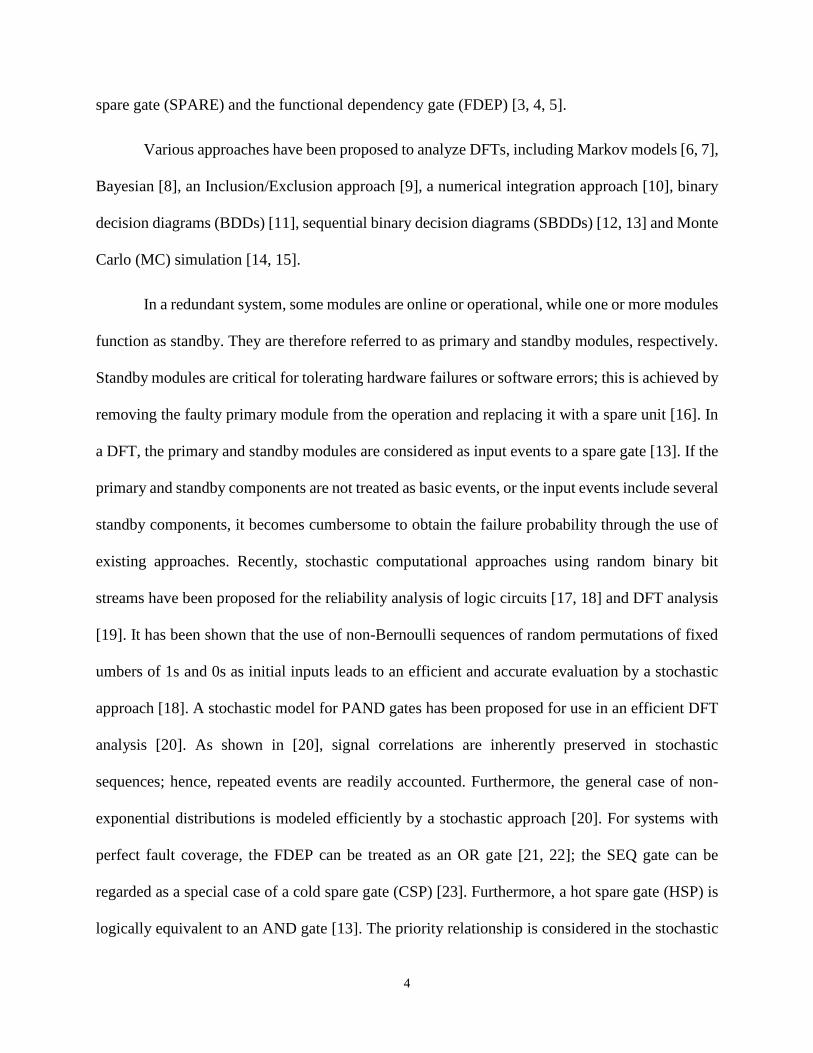
spare gate (SPARE) and the functional dependency gate (FDEP) [3, 4, 5].

Various approaches have been proposed to analyze DFTs, including Markov models [6, 7],

Bayesian [8], an Inclusion/Exclusion approach [9], a numerical integration approach [10], binary

decision diagrams (BDDs) [11], sequential binary decision diagrams (SBDDs) [12, 13] and Monte

Carlo (MC) simulation [14, 15].

In a redundant system, some modules are online or operational, while one or more modules

function as standby. They are therefore referred to as primary and standby modules, respectively.

Standby modules are critical for tolerating hardware failures or software errors; this is achieved by

removing the faulty primary module from the operation and replacing it with a spare unit [16]. In

a DFT, the primary and standby modules are considered as input events to a spare gate [13]. If the

primary and standby components are not treated as basic events, or the input events include several

standby components, it becomes cumbersome to obtain the failure probability through the use of

existing approaches. Recently, stochastic computational approaches using random binary bit

streams have been proposed for the reliability analysis of logic circuits [17, 18] and DFT analysis

[19]. It has been shown that the use of non-Bernoulli sequences of random permutations of fixed

umbers of 1s and 0s as initial inputs leads to an efficient and accurate evaluation by a stochastic

approach [18]. A stochastic model for PAND gates has been proposed for use in an efficient DFT

analysis [20]. As shown in [20], signal correlations are inherently preserved in stochastic

sequences; hence, repeated events are readily accounted. Furthermore, the general case of non-

exponential distributions is modeled efficiently by a stochastic approach [20]. For systems with

perfect fault coverage, the FDEP can be treated as an OR gate [21, 22]; the SEQ gate can be

regarded as a special case of a cold spare gate (CSP) [23]. Furthermore, a hot spare gate (HSP) is

logically equivalent to an AND gate [13]. The priority relationship is considered in the stochastic

5

PAND model of [20]; however, modeling of spare gates (and in particular, the warm spare gate

(WSP) and CSP), has not been considered. Hence, this paper focuses on the WSP and CSP gates.

A stochastic model is first proposed for spare gates in the analysis of DFTs; both exponential and

non-exponential (e.g. Weibull) distributions are then analyzed using this stochastic model.

In practice, the basic events of a system are often subject to common cause failures (CCFs)

including earthquakes, sudden changes in the environment, design errors and incorrect operations

[24]. CCFs are sometimes closely related; for instance, floods are likely to be caused by hurricanes.

These CCFs are referred to as dependent CCFs. Furthermore, the occurrence of a CCF is usually

not deterministic, but probabilistic, thus referred to as a probabilistic CCF (PCCF) [25]. The

probability of occurrence differs by components or conditions. The consideration of PCCFs in a

DFT analysis is of great significance as the system’s reliability is likely to be overestimated

without incorporating PCCFs. However, it presents a great challenge to consider PCCFs in a DFT

analysis using existing methods, such as an integration-based approach. In this paper, a stochastic

model is proposed for modeling the effect of dependent PCCFs. A general DFT with

independent/dependent PCCFs can be efficiently evaluated by the proposed stochastic approach.

The accuracy of a stochastic analysis increases with the length of the non-Bernoulli sequences in

stochastic computation. In summary, this paper makes the following novel contributions:

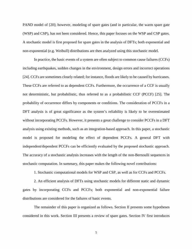
1. Stochastic computational models for WSP and CSP, as well as for CCFs and PCCFs.

2. An efficient analysis of DFTs using stochastic models for different static and dynamic

gates by incorporating CCFs and PCCFs; both exponential and non-exponential failure

distributions are considered for the failures of basic events.

The remainder of this paper is organized as follows. Section II presents some hypotheses

considered in this work. Section III presents a review of spare gates. Section IV first introduces

6

the fundamentals of the stochastic approach and a non-Bernoulli sequence generation algorithm;

then, stochastic models are proposed for spare gates, majority voters and CCFs/PCCFs. Several

benchmarks are simulated and analyzed in Section V. Finally, Section VI concludes the paper.

II. ASSUMPTIONS

The following assumptions are made in this paper:

The quantization level of a basic event is represented as a binary variable 𝑥, 𝑥 ∈ {0,1}, with

0 indicating no fault;

All basic events are fault-free at the beginning of the mission time;

The basic events are assumed to be non-repairable [26];

The failure probability of a component in a selected time interval [𝑡𝑖, 𝑡𝑖 + 𝛥𝑡] is considered

constant at the value at the beginning of the time interval, i.e., the failure probability is given

by 𝑝 = 𝐹(𝑡𝑖) for any time in the considered time interval. For simplicity, the time interval

[𝑡𝑖 , 𝑡𝑖 + 𝛥𝑡] is referred to as time 𝑖 in this paper.

III. REVIEW OF SPARE GATES

A standby system modeled by a spare gate usually consists of two types of modules: the

primary (or online) modules and the standby modules. Standby modules are used to replace the

faulty modules to keep the system functional or operational. Hence, the spare gate fires (i.e., fails)

if both of the modules fail. Spare gates are divided into three categories, depending on the

switching relationship of the primary and standby modules: the hot spare gate (HSP) [13, 26], the

cold spare gate (CSP) [13, 26], and the warm spare gate (WSP) [26, 27, 28, 29]. In an HSP system,

a standby module is always powered and ready to replace a faulty primary module when a fault

occurs. HSPs are typically used in systems, in which a minimal reconfiguration time is required,

7

e.g. a chemical process control system. In a CSP, however, the standby modules are usually not

powered until it is necessary to replace a faulty module [30]. Hence, it is usually used in power

consumption critical systems, such as a satellite system [16]. As a tradeoff between CSP and HSP,

the standby modules in a WSP are powered initially, but with a lower failure rate. The failure rate

of the standby module in a WSP changes when it is switched to replace a faulty module [27]. For

WSP, usually less power is consumed in the standby state compared to HSP, and less initialization

and recovery time are required compared to CSP [28, 29].

WSP

HSP

CSP

P S S

spare

P 10

10

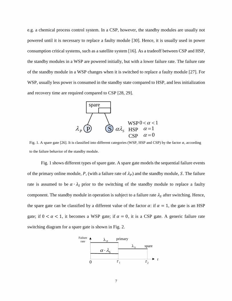
Fig. 1. A spare gate [26]. It is classified into different categories (WSP, HSP and CSP) by the factor 𝛼, according

to the failure behavior of the standby module.

Fig. 1 shows different types of spare gate. A spare gate models the sequential failure events

of the primary online module, 𝑃, (with a failure rate of 𝜆𝑃) and the standby module, 𝑆. The failure

rate is assumed to be 𝛼 ∙ 𝜆𝑆 prior to the switching of the standby module to replace a faulty

component. The standby module in operation is subject to a failure rate 𝜆𝑆 after switching. Hence,

the spare gate can be classified by a different value of the factor 𝛼: if 𝛼 = 1, the gate is an HSP

gate; if 0 < 𝛼 < 1, it becomes a WSP gate; if 𝛼 = 0, it is a CSP gate. A generic failure rate

switching diagram for a spare gate is shown in Fig. 2.

t

primary

0

Pλ

Sλ

Failure

rate

1 2

S spare

8

Fig. 2. A generic switching diagram for the failure in a spare gate [12, 26].

HSP and CSP gates can be regarded as special cases of the WSP gate; the only difference

lies in the value of the failure rate before and after the switching point. A spare gate can be

converted into a combinational fault tree with two sequential components serving as inputs of an

OR gate, as shown in Fig. 3 [12, 13].

G

G

(a) (b)

PS SP

SP

Fig. 3. The spare gate decomposition: (a) A combinational model for the spare gate, and (b) A simplified model

for CSP. " → " indicates an inclusive precedence in a failure order.

In Fig. 3, the sequential event 𝑆 → 𝑃 indicates that both modules fail and the standby

module fails before the primary module does; while the sequential event 𝑃 → 𝑆 means that both

modules fail and the primary module fails before the standby module. The two sequential events

cannot occur at the same time, thus they are mutually exclusive. Furthermore, it is impossible for

the standby module of a CSP gate to fail because the failure rate of the standby module before

switching is 0. Hence, the combinational model for a CSP gate can be simplified as shown in Fig.

3(b); this indicates that the output failure probability of a CSP gate is the same as the failure

probability of the sequential event 𝑃 → 𝑆. The output failure probability of the spare gate in Fig.

3(a) is given by [12]:

𝑈𝑠𝑦𝑠 = 𝑝(𝑃 → 𝑆) + 𝑝(𝑆 → 𝑃), (1)

9

while the probabilities of the two sequential failure events in (1) are given by:

𝑝(𝑃 → 𝑆) = ∫ ∫ 𝑓𝑃(𝜏2)𝑓𝑆,𝜆(𝜏1)𝑡−𝜏2

0

𝑡

0(1 − ∫ 𝑓𝑆,𝛼𝜆(𝜏1)𝑑𝜏1

𝜏2

0)𝑑𝜏2𝑑𝜏1, (2)

and

𝑝(𝑆 → 𝑃) = ∫ ∫ 𝑓𝑃(𝜏2)𝑓𝑆,𝛼𝜆(𝜏1)𝑡

𝜏1

𝑡

0𝑑𝜏2𝑑𝜏1, (3)

where 𝑓𝐴(𝑡), 𝑓𝑆,𝛼𝜆(𝑡) and 𝑓𝑆,𝜆(𝑡) are the failure probability density functions (pdfs) for the primary

module, the standby module before replacing the faulty primary module and after replacing the

faulty primary module. For a k-out-of-n WSP system consisting of identical WSPs, a closed

expression can be derived; however, it is only applicable to systems with identical input events

[31].

IV. PROPOSED STOCHASTIC MODELS

A. Stochastic Computation

Stochastic computation was initially proposed in the 1960s for reliable circuit design [32].

Probabilities are encoded into random binary bit streams by setting a proportional number of bits

to a specific value, i.e., 1 or 0. By using stochastic logic, Boolean logic operations are transformed

into probabilistic computations in the real domain. Stochastic computation has the advantages of

hardware simplicity and fault tolerance. However, inevitable random fluctuations occur in the

computation of probabilities. Conventionally, Bernoulli sequences are utilized as random binary

bit streams in stochastic computation. In a Bernoulli sequence, every bit is independently generated

as 1 or 0, according to a specified probability. For a probability of 0.5, this process is similar to a

coin-flipping experiment, i.e. a head or tail is observed for approximately half of the trials. Due to

its probabilistic nature, the number of 1s or 0s in a Bernoulli sequence is not deterministic, so

stochastic fluctuations exist in the computed result. [18] has shown that the use of non-Bernoulli

10

sequences of fixed numbers of 1s and 0s for the initial input probabilities significantly reduces the

effect of stochastic fluctuations compared to Bernoulli sequences. In this type of non-Bernoulli

sequences [18], the numbers of 1s and 0s are computed from a specified probability, and then they

are randomly permuted to encode the probability. This is a more efficient process compared to the

generation of Bernoulli sequences, because less pseudo-random numbers need to be generated.

The non-Bernoulli sequences contain deterministic numbers of 1s and 0s, so there is no variation

in the initial sequences. Therefore, the use of non-Bernoulli sequences as initial inputs results in

less variation in the stochastic computing process of a network, thus it produces more accurate

results than the case when Bernoulli sequences are used as initial inputs.

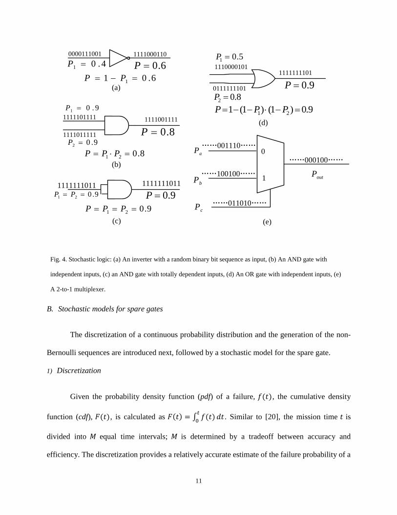
Examples of computation and encoding using non-Bernoulli sequences are shown in Fig.

4(a-d) for a sequence length of 10 bits; a longer sequence length is usually required in a practical

application, as shown in Fig. 4(e). For the 2-to-1 multiplexer of Fig. 4(e), the output takes the value

of one of the two inputs when the control bit is 0 or 1. When stochastic sequences are used as input

and control signals, this multiplexer selects one of the inputs as output according to the

distributions (and thus the probabilities) of 0s and 1s in the control sequence. In a stochastic

implementation, the multiplexer takes one of the inputs as output according to the probabilities

encoded in the distributions of the control bits.

Furthermore, the repeated input events (as typically encountered in an FTA) are readily

dealt with in a stochastic approach because a stochastic computing technique efficiently handles

the problem of signal re-convergence [20], as shown in Fig 4(c). The stochastic logic gates used

in this work are shown as follows:

11

1111101111

1111011111

1111001111

9.01 P

9.02 P

0111111101

8.02 P

9.0P

11111111011110000101

5.01 P

11111110119.021 PP

1111111011

(b)

(c)

(d)

8.021 PPP

9.0)1()1(1 21 PPP

9.021 PPP

9.0P

8.0P

0000111001 1111000110

4.01 P 6.0P

6.01 1 PP(a)

1

0

(e)

……000100……

……011010……

……100100……

……001110……aP

bP

cP

outP

Fig. 4. Stochastic logic: (a) An inverter with a random binary bit sequence as input, (b) An AND gate with

independent inputs, (c) an AND gate with totally dependent inputs, (d) An OR gate with independent inputs, (e)

A 2-to-1 multiplexer.

B. Stochastic models for spare gates

The discretization of a continuous probability distribution and the generation of the non-

Bernoulli sequences are introduced next, followed by a stochastic model for the spare gate.

1) Discretization

Given the probability density function (pdf) of a failure, 𝑓(𝑡), the cumulative density

function (cdf), 𝐹(𝑡), is calculated as 𝐹(𝑡) = ∫ 𝑓(𝑡)𝑡

0𝑑𝑡 . Similar to [20], the mission time 𝑡 is

divided into 𝑀 equal time intervals; 𝑀 is determined by a tradeoff between accuracy and

efficiency. The discretization provides a relatively accurate estimate of the failure probability of a

12

basic event with a reasonable 𝑀.

2) Generation of non-Bernoulli sequences

Let the failure probabilities for two adjacent time intervals, time 𝑖 − 1 and time 𝑖 , be

denoted by 𝑝𝑖−1 and 𝑝𝑖 respectively. Since the non-Bernoulli sequences use random permutations

of fixed numbers of 1s and 0s, for a sequence length of 𝐿 bits the number of 1s in the sequences

for the two failure probabilities are determined by 𝑁(𝑝𝑖−1) = 𝐿 ∙ 𝑝𝑖−1 and 𝑁(𝑝𝑖) = 𝐿 ∙ 𝑝𝑖

respectively. Let the non-Bernoulli sequence for the probability at time 𝑖 − 1 be represented by

𝑆(𝑝𝑖−1) , then the sequence 𝑆(𝑝𝑖) for the probability at time 𝑖 can be obtained by randomly

assigning a number of 1s to replace the 0s in 𝑆(𝑝𝑖−1); this number is given by 𝛥𝑁 = 𝑁(𝑝𝑖) −

𝑁(𝑝𝑖−1) = 𝐿 ∙ (𝑝𝑖 − 𝑝𝑖−1). The relationship between the two non-Bernoulli sequences for two

adjacent time intervals is then given by:

𝑆(𝑝𝑖) 𝐴𝑁𝐷 𝑆(𝑝𝑖−1) = 𝑆(𝑝𝑖−1). (4)

(4) is due to the assumption of non-reparability, such that the 1s in 𝑆(𝑝𝑖−1) still remain as 1s in

𝑆(𝑝𝑖); thus, the mutual set in both sequences is given by 𝑆(𝑝𝑖−1).

3) Stochastic model of the WSP/CSP gate

The failure probability of the spare gate with any inputs is given by (1); however, it is more

complex to derive the exact failure probability for non-exponentially distributed basic events.

Those are generally more realistic to model a basic event’s failure behavior in a mechanical system.

The derivation process becomes even more cumbersome when the primary and standby

components are combinations of several other events. Moreover, the components in a realistic DFT

system may also suffer from common cause failures that occur either deterministically or

probabilistically. This makes the distribution of the failure behavior even more complicated.

Hence, a stochastic model is proposed in this paper for efficiently analyzing spare gates.

13

Let 𝑆𝑖−1𝑃 and 𝑆𝑖

𝑃 denote the non-Bernoulli sequences generated for the failure probabilities

of the primary module at two adjacent time intervals 𝑖 − 1 and 𝑖, i.e., 𝐹𝑖−1𝑃 and 𝐹𝑖

𝑃, where 𝐹𝑃 is the

cdf for the failure of the primary module. As a primary module is non-repairable, the relationship

of (4) must be met. For the 𝑗th bit in the non-Bernoulli sequence, the state of the primary module

is given by 𝑆𝑖−1,𝑗𝑃 and 𝑆𝑖,𝑗

𝑃 for the two consecutive time intervals: a state of 0 or 1 indicates that no

fault occurs or a fault occurs. The state combination of the primary module at time 𝑖 − 1 and time

𝑖 for the 𝑗th trial – a trial is carried out by a bit or a combination of bits in the stochastic sequences

- is represented by 𝑆𝑖−1,𝑗𝑃 𝑆𝑖,𝑗

𝑃 , where 𝑆𝑖−1,𝑗𝑃 𝑆𝑖,𝑗

𝑃 ∈ {00, 01, 11} , due to the non-reparability

assumption. For the WSP/CSP gate, the failure rate of the standby module varies before and after

switching to replace the primary module (for CSP, the failure probability is 0 before switching).

Hence, it is necessary to record the failure time of the primary module to determine the failure

probability of the standby module. If 𝑆𝑘−1,𝑗𝑃 = 0 and 𝑆𝑘,𝑗

𝑃 = 1, it indicates that the primary module

fails at time 𝑘 for the 𝑗th trial; hence, for WSP and CSP, the operational time of the standby module

should be determined from the failure time of the primary module, i.e., 𝑡𝑠 = 𝑖 − 𝑘, where 𝑖 is the

present mission time and 𝑘 is the failure time of the primary module. Similarly, the operational

time of the standby module can be determined for any other trial.

Let 𝑆𝑖−1𝑆 and 𝑆𝑖

𝑆 be the stochastic sequences generated for the failure probabilities of the

standby module at two adjacent time intervals 𝑖 − 1 and 𝑖. Then we discuss the following three

different cases when 𝑆𝑖−1,𝑗𝑃 𝑆𝑖,𝑗

𝑃 = 00, 𝑆𝑖−1,𝑗𝑃 𝑆𝑖,𝑗

𝑃 = 01 and 𝑆𝑖−1,𝑗𝑃 𝑆𝑖,𝑗

𝑃 = 11:

For 𝑆𝑖−1,𝑗𝑃 𝑆𝑖,𝑗

𝑃 = 00, the primary module does not fail at time 𝑖. For a WSP, if 𝑆𝑖−1,𝑗𝑆 = 1,

then 𝑆𝑖,𝑗𝑆 = 1 . If 𝑆𝑖−1,𝑗

𝑆 = 0 , the current state of the standby module for the jth trial is

determined by the failure probability, i.e., the cdf 𝐹𝑖𝑆,𝛼𝜆

obtained from the failure rate of the

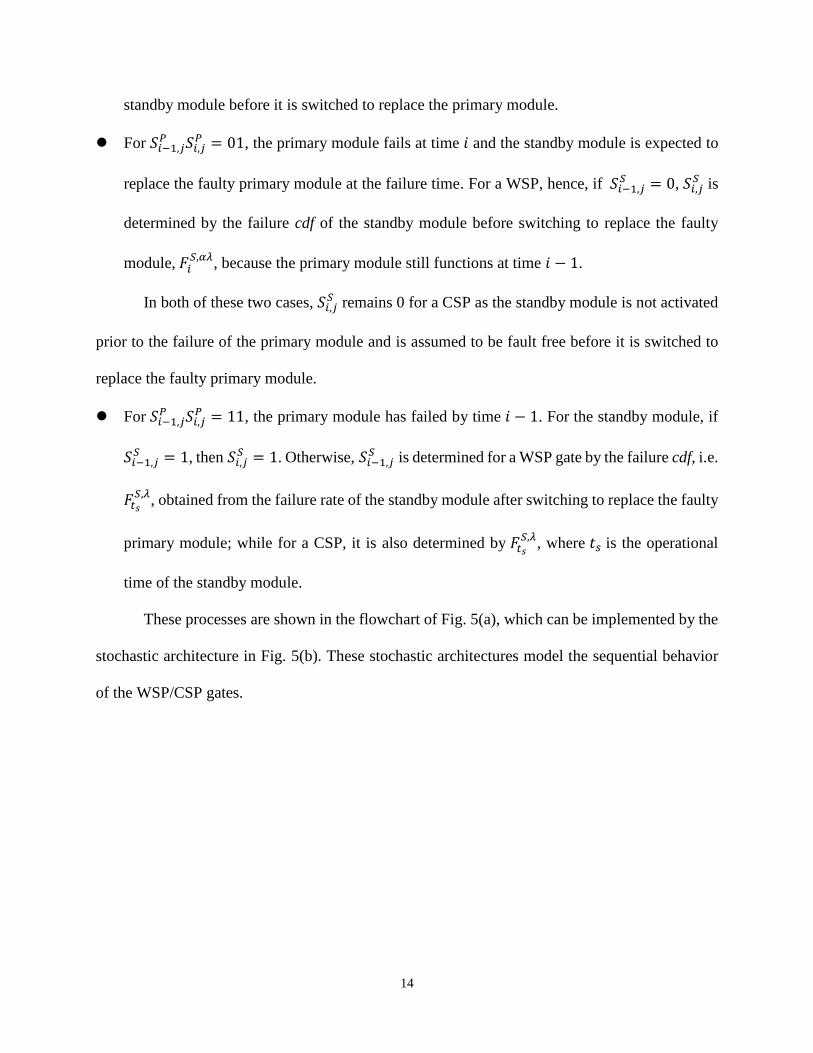
14

standby module before it is switched to replace the primary module.

For 𝑆𝑖−1,𝑗𝑃 𝑆𝑖,𝑗

𝑃 = 01, the primary module fails at time 𝑖 and the standby module is expected to

replace the faulty primary module at the failure time. For a WSP, hence, if 𝑆𝑖−1,𝑗𝑆 = 0, 𝑆𝑖,𝑗

𝑆 is

determined by the failure cdf of the standby module before switching to replace the faulty

module, 𝐹𝑖𝑆,𝛼𝜆

, because the primary module still functions at time 𝑖 − 1.

In both of these two cases, 𝑆𝑖,𝑗𝑆 remains 0 for a CSP as the standby module is not activated

prior to the failure of the primary module and is assumed to be fault free before it is switched to

replace the faulty primary module.

For 𝑆𝑖−1,𝑗𝑃 𝑆𝑖,𝑗

𝑃 = 11, the primary module has failed by time 𝑖 − 1. For the standby module, if

𝑆𝑖−1,𝑗𝑆 = 1, then 𝑆𝑖,𝑗

𝑆 = 1. Otherwise, 𝑆𝑖−1,𝑗𝑆 is determined for a WSP gate by the failure cdf, i.e.

𝐹𝑡𝑠

𝑆,𝜆, obtained from the failure rate of the standby module after switching to replace the faulty

primary module; while for a CSP, it is also determined by 𝐹𝑡𝑠

𝑆,𝜆, where 𝑡𝑠 is the operational

time of the standby module.

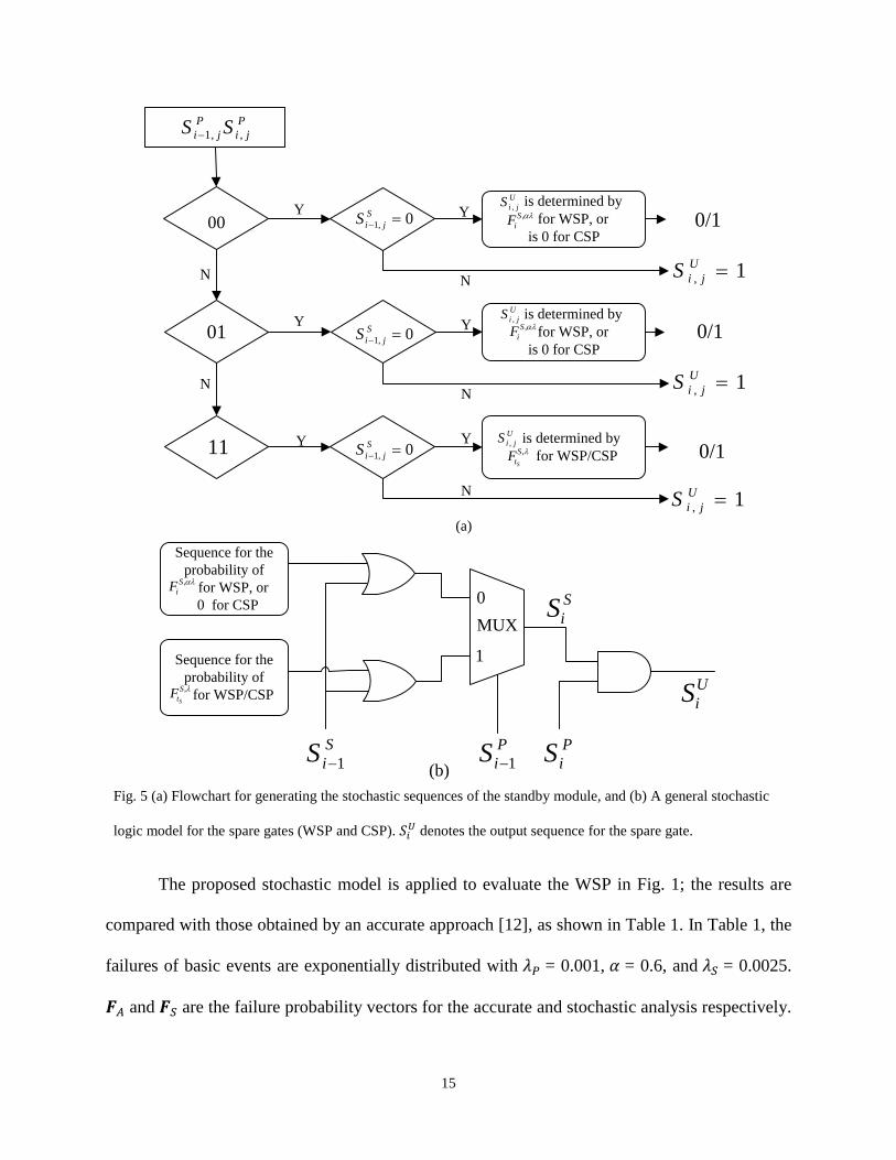
These processes are shown in the flowchart of Fig. 5(a), which can be implemented by the

stochastic architecture in Fig. 5(b). These stochastic architectures model the sequential behavior

of the WSP/CSP gates.

15

P

ji

P

ji SS ,,1

Y

N

Y

N

01Y

Y

N

N

11

Y

Y

N

is determined by

for WSP, or

is 0 for CSP

,S

iF

is determined by

for WSP/CSP

(a)

00

1, U

jiS

0/1

0/1

0/1

is determined by

for WSP, or

is 0 for CSP

0,1

S

jiS

0,1

S

jiS

0,1

S

jiS

1, U

jiS

1, U

jiS

U

jiS ,

U

jiS ,

U

jiS ,

,S

iF

,S

tSF

1

0

S

iS 1

MUX

(b)

Sequence for the

probability of

for WSP/CSP

Sequence for the

probability of

for WSP, or

0 for CSP

U

iS

P

iS 1

P

iS

S

iS

,S

iF

,S

tSF

Fig. 5 (a) Flowchart for generating the stochastic sequences of the standby module, and (b) A general stochastic

logic model for the spare gates (WSP and CSP). 𝑆𝑖𝑈 denotes the output sequence for the spare gate.

The proposed stochastic model is applied to evaluate the WSP in Fig. 1; the results are

compared with those obtained by an accurate approach [12], as shown in Table 1. In Table 1, the

failures of basic events are exponentially distributed with 𝜆𝑃 = 0.001, 𝛼 = 0.6, and 𝜆𝑆 = 0.0025.

𝑭𝐴 and 𝑭𝑆 are the failure probability vectors for the accurate and stochastic analysis respectively.

16

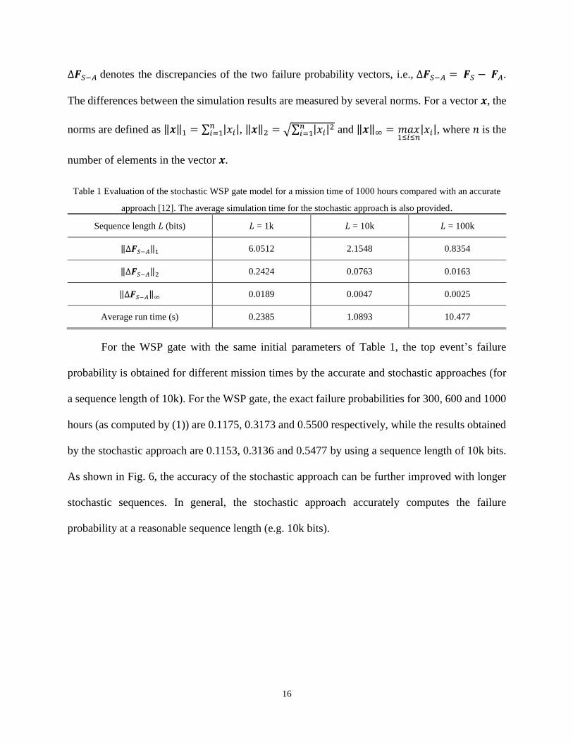
∆𝑭𝑆−𝐴 denotes the discrepancies of the two failure probability vectors, i.e., ∆𝑭𝑆−𝐴 = 𝑭𝑆 − 𝑭𝐴.

The differences between the simulation results are measured by several norms. For a vector 𝒙, the

norms are defined as ‖𝒙‖1 = ∑ |𝑥𝑖|𝑛𝑖=1 , ‖𝒙‖2 = √∑ |𝑥𝑖|2𝑛

𝑖=1 and ‖𝒙‖∞ = 𝑚𝑎𝑥1≤𝑖≤𝑛

|𝑥𝑖|, where 𝑛 is the

number of elements in the vector 𝒙.

Table 1 Evaluation of the stochastic WSP gate model for a mission time of 1000 hours compared with an accurate

approach [12]. The average simulation time for the stochastic approach is also provided.

Sequence length 𝐿 (bits) 𝐿 = 1k 𝐿 = 10k 𝐿 = 100k

‖∆𝑭𝑆−𝐴‖1 6.0512 2.1548 0.8354

‖∆𝑭𝑆−𝐴‖2 0.2424 0.0763 0.0163

‖∆𝑭𝑆−𝐴‖∞ 0.0189 0.0047 0.0025

Average run time (s) 0.2385 1.0893 10.477

For the WSP gate with the same initial parameters of Table 1, the top event’s failure

probability is obtained for different mission times by the accurate and stochastic approaches (for

a sequence length of 10k). For the WSP gate, the exact failure probabilities for 300, 600 and 1000

hours (as computed by (1)) are 0.1175, 0.3173 and 0.5500 respectively, while the results obtained

by the stochastic approach are 0.1153, 0.3136 and 0.5477 by using a sequence length of 10k bits.

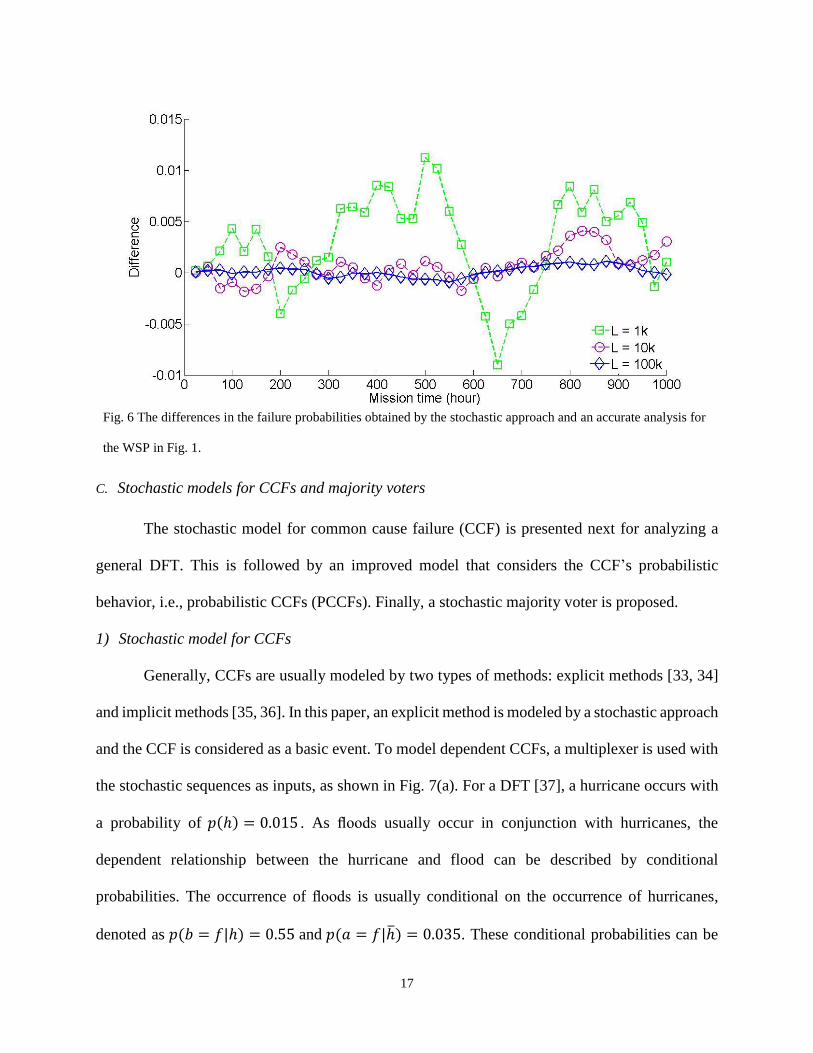
As shown in Fig. 6, the accuracy of the stochastic approach can be further improved with longer

stochastic sequences. In general, the stochastic approach accurately computes the failure

probability at a reasonable sequence length (e.g. 10k bits).

17

Fig. 6 The differences in the failure probabilities obtained by the stochastic approach and an accurate analysis for

the WSP in Fig. 1.

C. Stochastic models for CCFs and majority voters

The stochastic model for common cause failure (CCF) is presented next for analyzing a

general DFT. This is followed by an improved model that considers the CCF’s probabilistic

behavior, i.e., probabilistic CCFs (PCCFs). Finally, a stochastic majority voter is proposed.

1) Stochastic model for CCFs

Generally, CCFs are usually modeled by two types of methods: explicit methods [33, 34]

and implicit methods [35, 36]. In this paper, an explicit method is modeled by a stochastic approach

and the CCF is considered as a basic event. To model dependent CCFs, a multiplexer is used with

the stochastic sequences as inputs, as shown in Fig. 7(a). For a DFT [37], a hurricane occurs with

a probability of 𝑝(ℎ) = 0.015 . As floods usually occur in conjunction with hurricanes, the

dependent relationship between the hurricane and flood can be described by conditional

probabilities. The occurrence of floods is usually conditional on the occurrence of hurricanes,

denoted as 𝑝(𝑏 = 𝑓|ℎ) = 0.55 and 𝑝(𝑎 = 𝑓|ℎ̅) = 0.035. These conditional probabilities can be

18

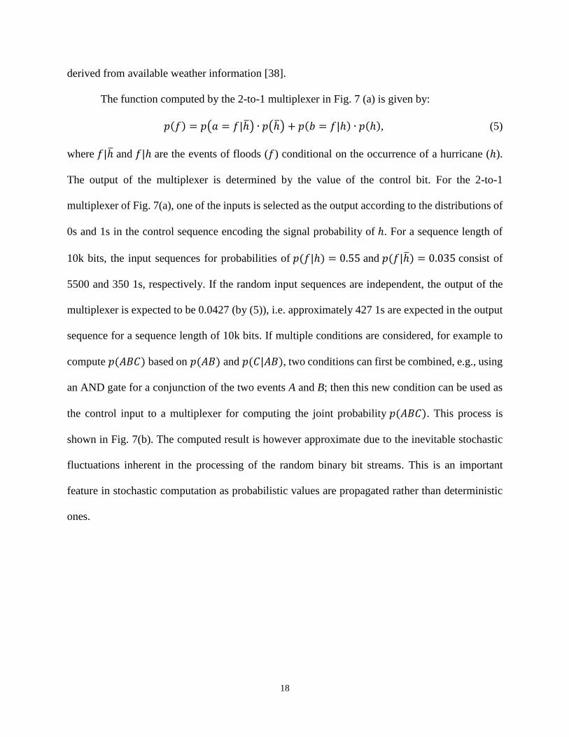
derived from available weather information [38].

The function computed by the 2-to-1 multiplexer in Fig. 7 (a) is given by:

𝑝(𝑓) = 𝑝(𝑎 = 𝑓|ℎ̅) ∙ 𝑝(ℎ̅) + 𝑝(𝑏 = 𝑓|ℎ) ∙ 𝑝(ℎ), (5)

where 𝑓|ℎ̅ and 𝑓|ℎ are the events of floods (𝑓) conditional on the occurrence of a hurricane (ℎ).

The output of the multiplexer is determined by the value of the control bit. For the 2-to-1

multiplexer of Fig. 7(a), one of the inputs is selected as the output according to the distributions of

0s and 1s in the control sequence encoding the signal probability of ℎ. For a sequence length of

10k bits, the input sequences for probabilities of 𝑝(𝑓|ℎ) = 0.55 and 𝑝(𝑓|ℎ̅) = 0.035 consist of

5500 and 350 1s, respectively. If the random input sequences are independent, the output of the

multiplexer is expected to be 0.0427 (by (5)), i.e. approximately 427 1s are expected in the output

sequence for a sequence length of 10k bits. If multiple conditions are considered, for example to

compute 𝑝(𝐴𝐵𝐶) based on 𝑝(𝐴𝐵) and 𝑝(𝐶|𝐴𝐵), two conditions can first be combined, e.g., using

an AND gate for a conjunction of the two events A and B; then this new condition can be used as

the control input to a multiplexer for computing the joint probability 𝑝(𝐴𝐵𝐶). This process is

shown in Fig. 7(b). The computed result is however approximate due to the inevitable stochastic

fluctuations inherent in the processing of the random binary bit streams. This is an important

feature in stochastic computation as probabilistic values are propagated rather than deterministic

ones.

19

fP

hP

1

0000100

001110

100100

011010

)|( hfbP

)|( hfaP )(outP

)( ABP

1

0

)|( ABCP

)|( ABCP

)( AP)(BP

(a) (b)

Fig. 7 (a) A stochastic multiplexer model for the dependency relationship between the two dependent CCFs of

flood (f) and hurricane (h), and (b) A stochastic model for computing the joint probabilities of multiple

conditions.

It has been shown in [18] that when the initial probabilities are encoded by non-Bernoulli

sequences, the stochastic fluctuations are significantly reduced compared with the use of Bernoulli

sequences. For the previous example, the occurrence probability of floods is obtained by using a

multiplexer with stochastic non-Bernoulli sequences; the mean and variance are reported in Table

2 for a number of simulations using different sequence lengths. As shown by the simulation results,

the evaluation accuracy is better for the stochastic approach with a smaller variance and it can be

improved with an increase of sequence length.

Table 2 Mean and variance of the occurrence probability of flood obtained by using the stochastic approach and

Monte Carlo (MC) method for 1,000 experiments with different sequence lengths or simulation runs.

Sequence length 𝐿 (bits) / Simulation runs

𝑁

𝑁/𝐿 = 1k 𝑁/𝐿 = 10k 𝑁/𝐿 = 100k

Stochastic approach Mean 0.04264 0.04274 0.04274

Variance 3.892 × 10−6 4.159 × 10−7 3.829 × 10−8

Monte Carlo

simulation

Mean 0.04284 0.04265 0.04271

Variance 5.5956 × 10−5 4.1978 × 10−6 4.0124 × 10−7

The stochastic approach efficiently computes the occurrence probability of dependent

CCFs as evidenced by the average run time in Table 2. Moreover, the variance is significantly

20

reduced with an increase of sequence length. The use of a sequence length of 1k bits generates

very accurate results, with a relative disparity (RD) of approximately 0.23%, compared to the

analytical result of 0.0427 computed by (5). RD is defined as:

𝑅𝐷 = (𝑝 − 𝑝0)/𝑝0, (6)

where 𝑝 and 𝑝0 are the probabilities obtained by using the stochastic approach and an accurate

analysis, respectively. For an increased sequence length, a smaller RD can be obtained by the

stochastic approach.

2) A stochastic model for PCCF

A mechanical system can be subject to multiple CCFs, as denoted by 𝐶𝐶𝐹1, 𝐶𝐶𝐹2, ⋯,𝐶𝐶𝐹𝑚.

The failure of a dependent event affected by a specific CCF (say 𝐶𝐶𝐹𝑖 ) occurs with certain

probability, so the CCF is considered as a probabilistic CCF (PCCF). The occurrence probability

of a PCCF is given by 𝛾𝑖 = 𝑝(𝐷𝑒𝑝𝑒𝑛𝑑𝑒𝑛𝑡 𝑒𝑣𝑒𝑛𝑡 𝑓𝑎𝑖𝑙𝑠|𝐶𝐶𝐹𝑖 𝑜𝑐𝑐𝑢𝑟𝑠); 𝛾𝑖 may vary for different

components affected by a CCF.

PCCFCCF

(a) (c)

factor

pp

1S 2S nS

1 2 ni ibS

iaS

ibS

iS

(b)

iaS

iS

Fig. 8 (a) A PCCF gate [25], (b) a combinational model for the PCCF gate, and (c) proposed stochastic model for

the PCCF gate.

In Fig. 8(a), the CCF occurs as a trigger event with probability p; then one or more dependent

events affected by the trigger event fail at a specific probability. For example, an event 𝑆𝑖 occurs

21

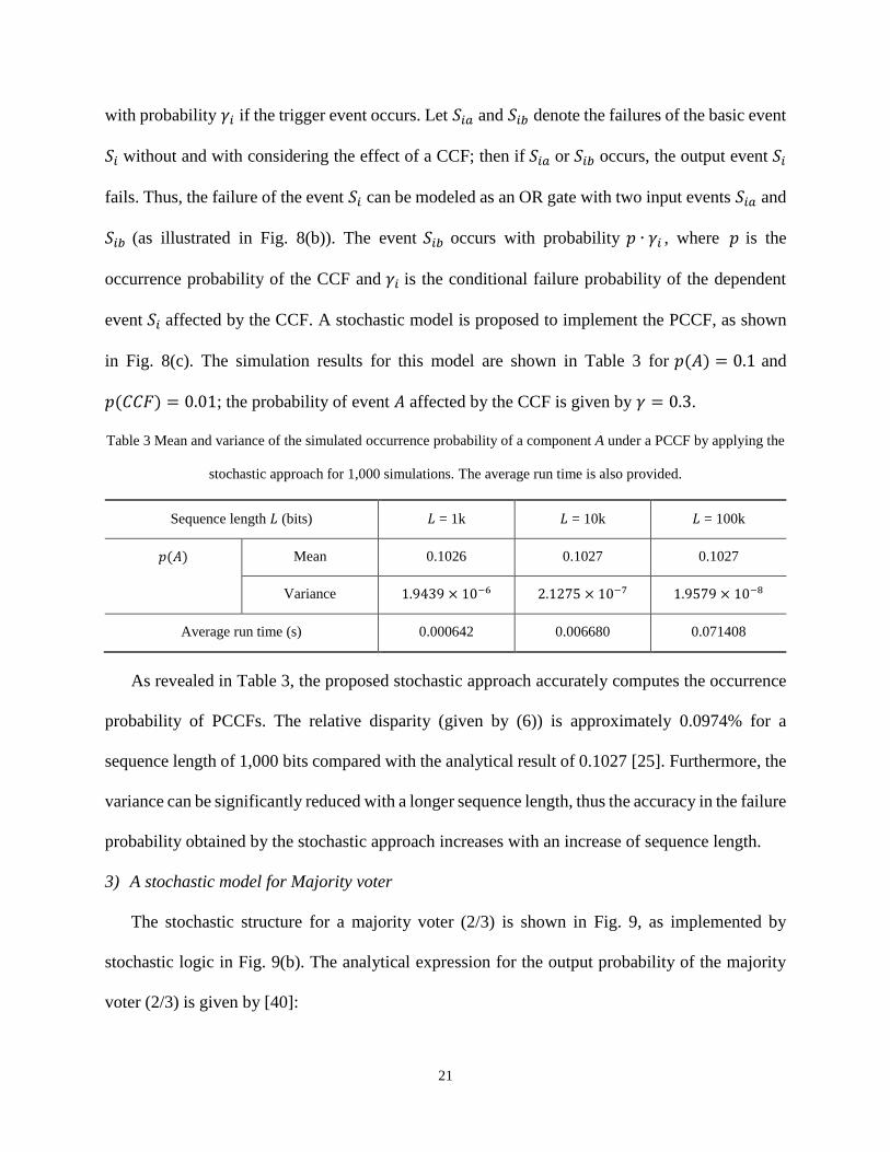
with probability 𝛾𝑖 if the trigger event occurs. Let 𝑆𝑖𝑎 and 𝑆𝑖𝑏 denote the failures of the basic event

𝑆𝑖 without and with considering the effect of a CCF; then if 𝑆𝑖𝑎 or 𝑆𝑖𝑏 occurs, the output event 𝑆𝑖

fails. Thus, the failure of the event 𝑆𝑖 can be modeled as an OR gate with two input events 𝑆𝑖𝑎 and

𝑆𝑖𝑏 (as illustrated in Fig. 8(b)). The event 𝑆𝑖𝑏 occurs with probability 𝑝 ∙ 𝛾𝑖 , where 𝑝 is the

occurrence probability of the CCF and 𝛾𝑖 is the conditional failure probability of the dependent

event 𝑆𝑖 affected by the CCF. A stochastic model is proposed to implement the PCCF, as shown

in Fig. 8(c). The simulation results for this model are shown in Table 3 for 𝑝(𝐴) = 0.1 and

𝑝(𝐶𝐶𝐹) = 0.01; the probability of event 𝐴 affected by the CCF is given by 𝛾 = 0.3.

Table 3 Mean and variance of the simulated occurrence probability of a component A under a PCCF by applying the

stochastic approach for 1,000 simulations. The average run time is also provided.

Sequence length 𝐿 (bits) 𝐿 = 1k 𝐿 = 10k 𝐿 = 100k

𝑝(𝐴) Mean 0.1026 0.1027 0.1027

Variance 1.9439 × 10−6 2.1275 × 10−7 1.9579 × 10−8

Average run time (s) 0.000642 0.006680 0.071408

As revealed in Table 3, the proposed stochastic approach accurately computes the occurrence

probability of PCCFs. The relative disparity (given by (6)) is approximately 0.0974% for a

sequence length of 1,000 bits compared with the analytical result of 0.1027 [25]. Furthermore, the

variance can be significantly reduced with a longer sequence length, thus the accuracy in the failure

probability obtained by the stochastic approach increases with an increase of sequence length.

3) A stochastic model for Majority voter

The stochastic structure for a majority voter (2/3) is shown in Fig. 9, as implemented by

stochastic logic in Fig. 9(b). The analytical expression for the output probability of the majority

voter (2/3) is given by [40]:

22

𝑝(𝑂𝑢𝑡) = 𝑝(𝐴) ∙ 𝑝(𝐵) + 𝑝(𝐴) ∙ 𝑝(𝐶) + 𝑝(𝐵) ∙ 𝑝(𝐶) − 2 ∙ 𝑝(𝐴) ∙ 𝑝(𝐵) ∙ 𝑝(𝐶) (7)

A

C

B

A

C

B 2/3

(a) (b)

OutOut

Fig. 9 (a) A majority voter (2/3) [40]; (b) A stochastic model for the majority voter (2/3).

Table 4 Mean and variance of the failure probabilities of 2/3 and 3/5 majority voters, obtained by the stochastic

approach. The average simulation time is also provided.

For 2/3 voter, 𝑝(𝐴) = 0.3, 𝑝(𝐵) = 0.6, 𝑝(𝐶) = 0.2

Sequence length L (bits) 𝐿 = 1k 𝐿 = 10k 𝐿 = 100k

Mean 0.2882 0.2880 0.2880

Variance 6.3098 × 10−5 5.4278 × 10−6 5.8191 × 10−7

Average simulation time (s) 0.002396 0.002264 0.013988

For 3/5 voter, 𝑝(𝐴) = 0.2, 𝑝(𝐵) = 0.4, 𝑝(𝐶) = 0.5, 𝑝(𝐷) = 0.1, 𝑝(𝐸) = 0.4

Sequence length 𝐿 (bits) 𝐿 = 1k 𝐿 = 10k 𝐿 = 100k

Mean 0.1783 0.1781 0.1780

Variance 6.6767 × 10−5 6.2741 × 10−6 6.3871 × 10−7

Average simulation time (s) 0.003154 0.027721 0.281911

For a (2/3) majority voter with inputs’ failure probabilities given in Table 4, the output failure

probability is 0.2880 by (7); the relative disparity (RD) is 0.069% (given by (6)) for the stochastic

approach using sequences of 1k bits. For a (3/5) majority voter, the output probability is 0.1780

using the analysis of [40], while the RD is approximately 0.17% for the stochastic approach with

23

𝐿 = 1k bits. Thus, the error in the failure probability for the stochastic approach decreases with

the increase of sequence length. Similar stochastic circuits can be constructed for majority gates

with more than three inputs.

D. DFT analysis flow

Following the proposed stochastic models for the spare and PAND gates [20], the process for

evaluating the top event’s failure probability of a general DFT with PCCFs, consists of the

following steps:

i. Replace the original spare gate with the proposed stochastic model for WSP/CSP in Fig. 5(b);

ii. Substitute the original FDEP and PAND gates with the OR model [21, 22] and the stochastic

PAND model in [20] respectively; then a DFT with dynamic gates can be implemented by

combinational logic;

iii. Encode the events’ failure probabilities at different time steps into non-Bernoulli sequences;

iv. If PCCFs are considered in the DFT, an additional PCCF module is required for each of the

basic events subject to PCCFs. Moreover, if the CCFs are dependent, a stochastic multiplexer

is used to model the effect of the dependency.

v. Derive the top event’s failure probability at different time steps by propagating the non-

Bernoulli sequences through the stochastic models.

V. CASE STUDIES

In this section, several case studies are presented to show the efficiency and accuracy of the

stochastic method, in comparison with the analytical method of [10] and the Monte Carlo (MC)

approach of [15]. Simulations are performed for DFTs with and without probabilistic common

cause failures (PCCFs). Furthermore, the effect of dependent PCCFs is also analyzed. Non-

exponential distributions of the basic events are also considered to show the capabilities of the

24

stochastic approach to handle general cases. All simulations are run on a computer with a 3.10

GHz i3-2100 microprocessor and a 6 GB memory.

Let the failure probability of a basic event 𝐵 at time 𝑖 be 𝐹𝑖𝐵, 𝑖 ∈ {1, 2, ⋯ , 𝑀}, obtained as the

failure cdf for the basic event; then the failure probability of the DFT is given by:

𝐹(𝑖) = 𝑓(𝐹𝑖𝐵), (8)

where 𝑓(. ) indicates the logic operation determined by the system’s topology. Hence, the failure

probability vector for the entire mission time is given by a vector 𝑭 = (𝐹(1), 𝐹(2), ⋯ , 𝐹(𝑀)),

where 𝑀 indicates the number of discretized intervals of the mission time. The failure probability

vectors obtained using the stochastic, analytical [10] and MC [15] approaches are then represented

by 𝑭𝑆, 𝑭𝐴 and 𝑭𝑀𝐶 respectively. Hence, ∆𝑭𝑆−𝐴 indicates the disparity vector for the stochastic and

analytical methods; ∆𝑭𝑀𝐶−𝐴 represents the disparity vector for the MC and analytical approaches.

Similarly, the norms, ‖∙‖1, ‖∙‖2 and ‖∙‖∞, are used to measure the differences of these failure

probability vectors.

A. HECS with and without PCCFs

A DFT of the Hypothetical Example Computer System (HECS) (from [26] and shown in Fig.

10) is used to illustrate the efficiency and accuracy of the proposed stochastic method.

A1 A2Cold

Spare AMemory

Interface Unit1

Memory

Interface Unit2

Operator console

Operator & software

M1 M2 M3 M4 M5

Redundant bus

Fig. 10 The Hypothetical Example Computer System (HECS) [26].

25

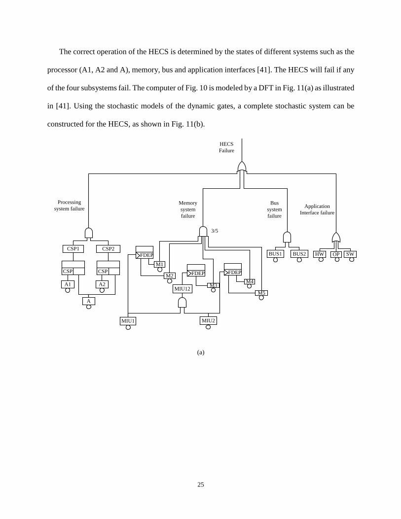
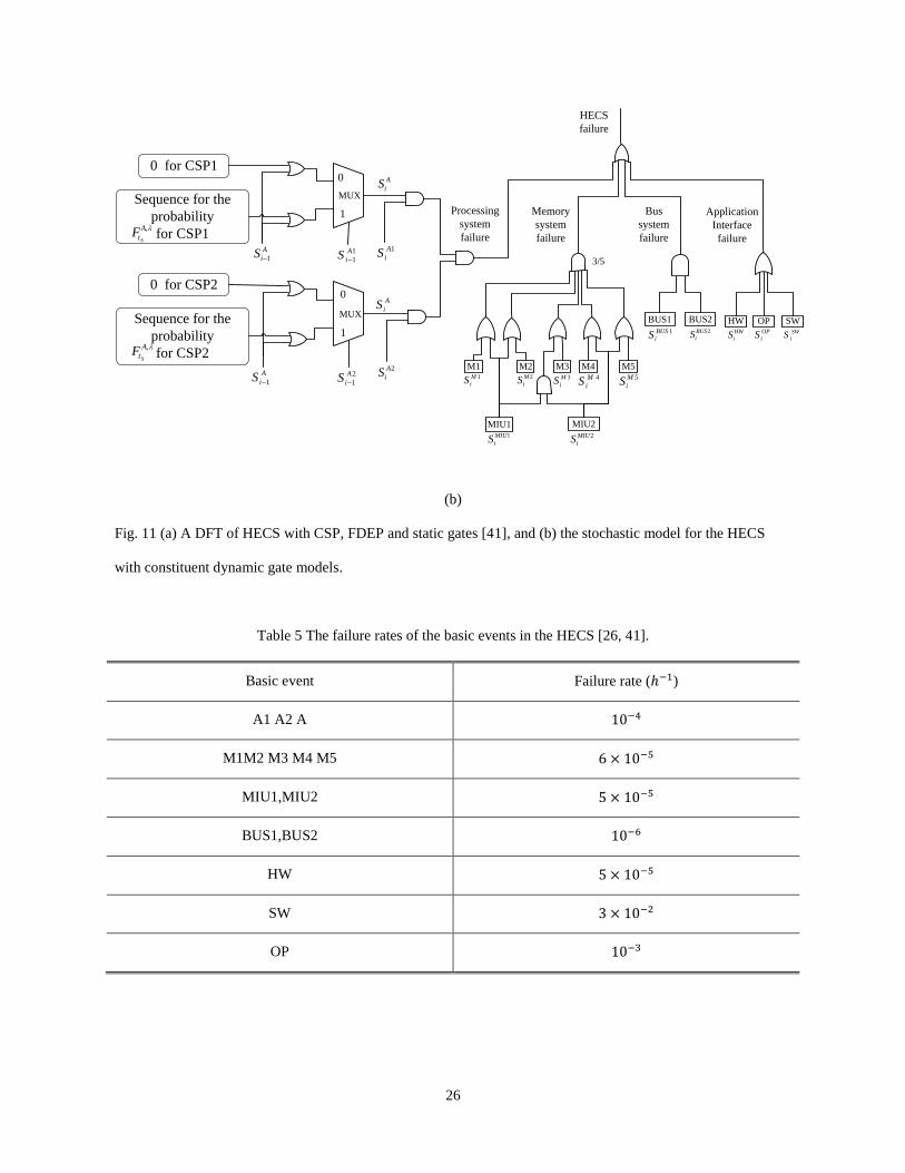
The correct operation of the HECS is determined by the states of different systems such as the

processor (A1, A2 and A), memory, bus and application interfaces [41]. The HECS will fail if any

of the four subsystems fail. The computer of Fig. 10 is modeled by a DFT in Fig. 11(a) as illustrated

in [41]. Using the stochastic models of the dynamic gates, a complete stochastic system can be

constructed for the HECS, as shown in Fig. 11(b).

CSP1 CSP2

CSP

A1

A

A2

CSP

3/5

HW OP SWBUS1 BUS2FDEP

M1

MIU1 MIU2

M2

MIU12M3

M4

M5

FDEP FDEP

Memory

system

failure

Bus

system

failure

Application

Interface failure

Processing

system failure

HECS

Failure

(a)

26

3/5

HECS

failure

Memory

system

failure

Bus

system

failure

Application

Interface

failure

BUS1 BUS2 HW SWOP

M5

MIU2MIU1

M2 M3 M4M1

Processing

system

failure

11

00

01A

iS

0 for CSP2

1

0

MUXSequence for the

probability

for CSP1

0 for CSP1

Sequence for the

probability

for CSP2

1

0

MUX

1M

iS

1MIU

iS 2MIU

iS

2M

iS 3M

iS 4M

iS 5M

iS

1BUS

iS2BUS

iS HW

iSOP

iS SW

iS

A

iS

1A

iS

A

iS 12

1

A

iS

A

iS 1

2A

iS

1

1

A

iS

,A

tSF

,A

tSF

(b)

Fig. 11 (a) A DFT of HECS with CSP, FDEP and static gates [41], and (b) the stochastic model for the HECS

with constituent dynamic gate models.

Table 5 The failure rates of the basic events in the HECS [26, 41].

Basic event Failure rate (ℎ−1)

A1 A2 A 10−4

M1M2 M3 M4 M5 6 × 10−5

MIU1,MIU2 5 × 10−5

BUS1,BUS2 10−6

HW 5 × 10−5

SW 3 × 10−2

OP 10−3

27

The mission time of the HECS is assumed to be 100 hours and the failure behaviors of the

basic events in the HECS are considered to be exponentially distributed (the failure rates are shown

in Table 5 [26, 41]).

For a mission time of 100 hours, the difference in failure probabilities of the HECS and the

average simulation time are shown in Table 6 for the different approaches. 𝑁 and 𝐿 denote the

number of simulation runs for the MC method and the sequence length for the stochastic approach,

respectively. The norms of the disparity vectors are presented for the stochastic and MC [15]

approaches.

Table 6 Norms of the differences in the top event’s failure probability vectors obtained by the proposed stochastic

approach and MC simulation for the DFT in Example A. The average run time is also provided.

𝑁/𝐿 = 1k 𝑁/𝐿 = 10k 𝑁/𝐿 = 100k

‖∆𝑭𝑆−𝐴‖1 0.1749 0.0529 0.0168

‖∆𝑭𝑆−𝐴‖2 0.0225 0.0066 0.0023

‖∆𝑭𝑆−𝐴‖∞ 0.0064 0.0016 7.0872 × 10−4

‖∆𝑭𝑀𝐶−𝐴‖1 0.8199 0.2830 0.1024

‖∆𝑭𝑀𝐶−𝐴‖2 0.1079 0.0386 0.0140

‖∆𝑭𝑀𝐶−𝐴‖∞ 0.0364 0.0134 0.0049

Average run

time (s)

Accurate Analysis 0.001738

Stochastic 0.0509 0.3868 3.9639

MC 0.1414 1.2583 12.596

As shown in Table 6, the proposed stochastic approach requires a shorter run time and results

in a smaller variance in the computed failure probability; hence, it is more efficient and more

accurate than the MC method. The evaluation accuracy can be further improved by increasing the

28

sequence length 𝐿. However, a trade-off between precision and efficiency must be determined

when selecting the sequence length. Although the accurate analysis results in the shortest run time,

the significantly longer time required for deriving the analytical expressions is not included in the

value reported in Table 6.

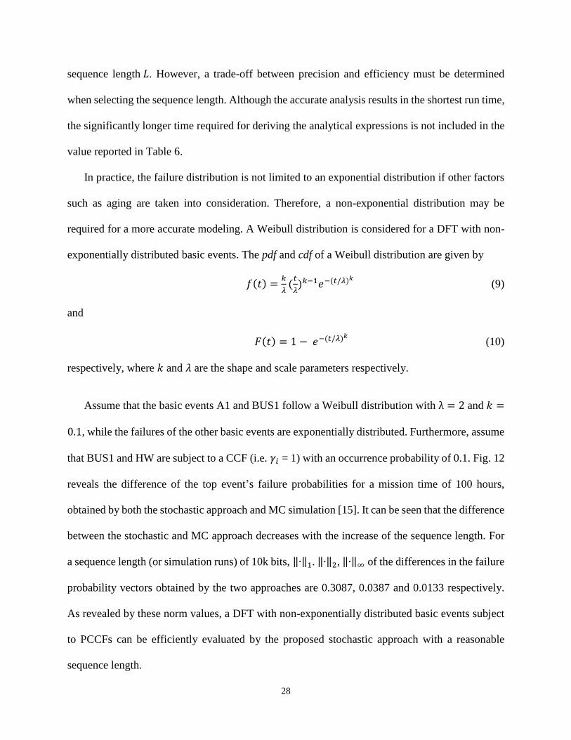
In practice, the failure distribution is not limited to an exponential distribution if other factors

such as aging are taken into consideration. Therefore, a non-exponential distribution may be

required for a more accurate modeling. A Weibull distribution is considered for a DFT with non-

exponentially distributed basic events. The pdf and cdf of a Weibull distribution are given by

𝑓(𝑡) =𝑘

𝜆(

𝑡

𝜆)𝑘−1𝑒−(𝑡/𝜆)𝑘

(9)

and

𝐹(𝑡) = 1 − 𝑒−(𝑡/𝜆)𝑘 (10)

respectively, where 𝑘 and 𝜆 are the shape and scale parameters respectively.

Assume that the basic events A1 and BUS1 follow a Weibull distribution with λ = 2 and 𝑘 =

0.1, while the failures of the other basic events are exponentially distributed. Furthermore, assume

that BUS1 and HW are subject to a CCF (i.e. 𝛾𝑖 = 1) with an occurrence probability of 0.1. Fig. 12

reveals the difference of the top event’s failure probabilities for a mission time of 100 hours,

obtained by both the stochastic approach and MC simulation [15]. It can be seen that the difference

between the stochastic and MC approach decreases with the increase of the sequence length. For

a sequence length (or simulation runs) of 10k bits, ‖∙‖1. ‖∙‖2, ‖∙‖∞ of the differences in the failure

probability vectors obtained by the two approaches are 0.3087, 0.0387 and 0.0133 respectively.

As revealed by these norm values, a DFT with non-exponentially distributed basic events subject

to PCCFs can be efficiently evaluated by the proposed stochastic approach with a reasonable

sequence length.

29

Fig. 12 Difference in the failure probabilities of the top event for the HECS for a mission time of 100 hours.

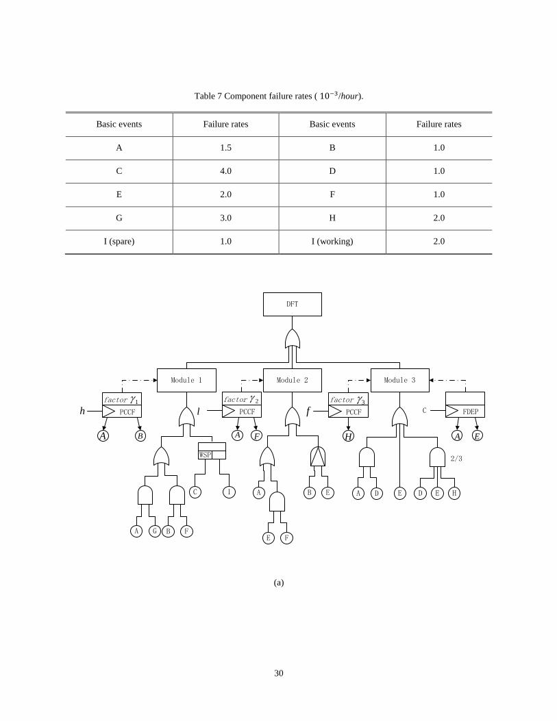
B. DFT with dependent PCCFs

A DFT with WSP, FDEP and PAND gates is analyzed next to show the efficiency of the

stochastic approach (Fig. 13(a)). Assume that ℎ, 𝑙 and 𝑓 denote the events of hurricanes, lightning

strikes and floods respectively. Table 7 shows the exponentially distributed failure rates of the

components; non-exponential distributions will be dealt with subsequently. The occurrence

probabilities of a hurricane and a lightning strike are given as 𝑝(ℎ) = 0.015 and 𝑝(𝑙) = 0.025

respectively. The dependencies between the CCFs are given as the conditional probabilities

between a hurricane and floods, i.e., 𝑝(𝑓|ℎ) = 0.55 and 𝑝(𝑓|ℎ̅) = 0.035 as obtained from

weather information [38]. The probability of a component affected by a CCF is assumed to be

𝛾𝑖 = 0.8 for 𝑖 = 1, 2, 3 (where 𝑖 indicates a different CCF, i.e., ℎ, 𝑙, 𝑓, respectively). For this

DFT, a stochastic model is constructed in Fig. 13(b) with the PAND model of [20] and the

stochastic models in Figs. 7 and 8 for considering the effects of PCCFs.

30

Table 7 Component failure rates ( 10−3/hour).

Basic events Failure rates Basic events Failure rates

A 1.5 B 1.0

C 4.0 D 1.0

E 2.0 F 1.0

G 3.0 H 2.0

I (spare) 1.0 I (working) 2.0

DFT

Module 1 Module 2 Module 3

C I

B FA G

A B E

E F

A D HD E E

2/3

PCCF

factor

A B

PCCF

factor

A F

PCCF

factor

H

FDEP

A E

f32

Clh1

WSP

(a)

31

DFT

E

D

f

3

hP

1

0)|( hfP

)|( hfP

F

G

h

1

A

B

A F

1

0

I

iS 1

MUXSequence for

the probability

for WSP

Sequence for

the probability

for WSP,I

iF

Module 1 Module 2

G

iS

F

iS

A

iS

B

iS l2

A C E

Module 3

H

,I

tSF

I

iS

C

iSC

iS 1

h

iS

1

iS

2

iS

A

iSA

iSF

iS

l

iS

E

iS OUT

iS 1

OUT

iS

E

iS E

iS 1

B

iS

E

iSC

iS

D

iS

H

iS

h

iS

hf

iS |

hf

iS |

f

iS

3

iS

(b)

Fig. 13 (a) A DFT with dependent PCCFs (taken from [24]), and (b) a stochastic model for the DFT in (a).

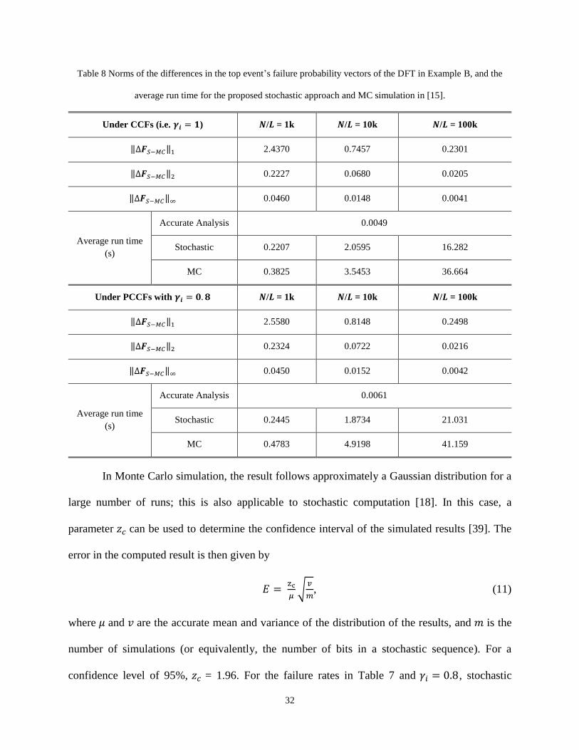
The average run time and norms of the differences in the failure probability vectors of the DFT

obtained by the stochastic and MC [15] approaches are given in Table 8 for a mission time of 200

hours. Also shown are the failure probabilities by considering PCCFs for each of the modules.

32

Table 8 Norms of the differences in the top event’s failure probability vectors of the DFT in Example B, and the

average run time for the proposed stochastic approach and MC simulation in [15].

Under CCFs (i.e. 𝜸𝒊 = 𝟏) 𝑵/𝑳 = 1k 𝑵/𝑳 = 10k 𝑵/𝑳 = 100k

‖∆𝑭𝑆−𝑀𝐶‖1 2.4370 0.7457 0.2301

‖∆𝑭𝑆−𝑀𝐶‖2 0.2227 0.0680 0.0205

‖∆𝑭𝑆−𝑀𝐶‖∞ 0.0460 0.0148 0.0041

Average run time

(s)

Accurate Analysis 0.0049

Stochastic 0.2207 2.0595 16.282

MC 0.3825 3.5453 36.664

Under PCCFs with 𝜸𝒊 = 𝟎. 𝟖 𝑵/𝑳 = 1k 𝑵/𝑳 = 10k 𝑵/𝑳 = 100k

‖∆𝑭𝑆−𝑀𝐶‖1 2.5580 0.8148 0.2498

‖∆𝑭𝑆−𝑀𝐶‖2 0.2324 0.0722 0.0216

‖∆𝑭𝑆−𝑀𝐶‖∞ 0.0450 0.0152 0.0042

Average run time

(s)

Accurate Analysis 0.0061

Stochastic 0.2445 1.8734 21.031

MC 0.4783 4.9198 41.159

In Monte Carlo simulation, the result follows approximately a Gaussian distribution for a

large number of runs; this is also applicable to stochastic computation [18]. In this case, a

parameter 𝑧𝑐 can be used to determine the confidence interval of the simulated results [39]. The

error in the computed result is then given by

𝐸 = zc

𝜇√

𝑣

𝑚, (11)

where 𝜇 and 𝑣 are the accurate mean and variance of the distribution of the results, and 𝑚 is the

number of simulations (or equivalently, the number of bits in a stochastic sequence). For a

confidence level of 95%, 𝑧𝑐 = 1.96. For the failure rates in Table 7 and 𝛾𝑖 = 0.8, stochastic

33

sequences of one million bits are used to find the accurate mean and variance, as 0.8119 and 0.1527,

respectively, for the stochastic approach. For a sequence length of 10k, the error is then obtained

by (11) as 0.9434% (i.e. less than 1%) at a confidence level of 95%. As per (11), the error decreases

with an increase of sequence length at a given confidence level. The required sequence length can

thus be estimated by (11) for achieving a desired evaluation accuracy.

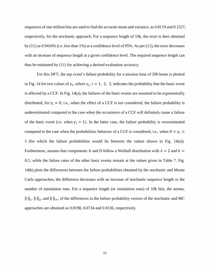
For this DFT, the top event’s failure probability for a mission time of 200 hours is plotted

in Fig. 14 for two values of 𝛾𝑖, where 𝛾𝑖, 𝑖 = 1, 2, 3, indicates the probability that the basic event

is affected by a CCF. In Fig. 14(a), the failures of the basic events are assumed to be exponentially

distributed; for γi = 0, i.e., when the effect of a CCF is not considered, the failure probability is

underestimated compared to the case when the occurrence of a CCF will definitely cause a failure

of the basic event (i.e. when 𝛾𝑖 = 1). In the latter case, the failure probability is overestimated

compared to the case when the probabilistic behavior of a CCF is considered, i.e., when 0 < 𝛾𝑖 <

1 (for which the failure probabilities would lie between the values shown in Fig. 14(a)).

Furthermore, assume that components A and D follow a Weibull distribution with 𝜆 = 2 and 𝑘 =

0.1, while the failure rates of the other basic events remain at the values given in Table 7. Fig.

14(b) plots the differences between the failure probabilities obtained by the stochastic and Monte

Carlo approaches; the difference decreases with an increase of stochastic sequence length or the

number of simulation runs. For a sequence length (or simulation runs) of 10k bits, the norms,

‖∙‖1. ‖∙‖2, and ‖∙‖∞, of the differences in the failure probability vectors of the stochastic and MC

approaches are obtained as 0.8198, 0.0734 and 0.0136, respectively.

34

(a)

(b)

Fig. 14 Example B: (a) Failure probability of the DFT subject to PCCFs for 𝛾𝑖 = 0 and 𝛾𝑖 = 1 (for basic events

with exponentially distributed failures, using a sequence length of 10k bits), and (b) Difference of the failure

35

probabilities of the DFT subject to PCCFs for 𝛾𝑖 = 0.8 (for basic events with non-exponentially distributed

failures).

As can be seen from these results, the DFT systems (inclusive of the spare gate, PAND and

FDEP gates) can be efficiently evaluated by the proposed stochastic approach. The stochastic

approach is more efficient than a MC method [15] with an equivalent number of simulation runs.

Furthermore, the accuracy of the proposed stochastic approach can be improved by increasing the

sequence length. The required sequence length is determined as a trade-off between precision and

efficiency. It is also shown that the reliability of a DFT system decreases by considering the effects

of PCCFs that widely occur in practice. Hence, if the failure of certain component affected by

PCCFs is not considered, the reliability of a DFT is likely to be overestimated. If the effect of

PCCFs is considered to be deterministic in causing a failure, then the reliability of a DFT is

underestimated.

VI. CONCLUSION

In this paper, stochastic models have been proposed for analyzing a two-input spare gate and

probabilistic common cause failures (PCCFs) in a dynamic fault tree (DFT); the WSP and CSP

gates have been analyzed in detail. For a DFT with spare gates, a stochastic approach using the

proposed models provides an efficient analysis of the DFT compared to an analytical approach.

The use of non-Bernoulli sequences of random permutations of fixed numbers of 1s and 0s as

initial input probabilities makes the stochastic approach more efficient and more accurate than

Monte Carlo simulation. The effect of PCCF has been taken into consideration and a stochastic

logic model has been constructed for dependent PCCFs. The efficiency and accuracy of the

proposed stochastic approach have been shown by the case studies of several benchmark systems.

36

Ongoing work includes the stochastic modeling of repair schemes and the assessment of

multiple-valued DFT systems with imperfect fault coverage.

REFERENCES

[1] A. Clifton Ericson II.: Fault tree analysis – a history. In Proceedings of the 17th International System Safety Conference,

August 16–21, 1999.

[2] N. G. .Leveson.: Safeware: System safety and computers.: Addison-Wesley, 1995.

[3] M. A. Boyd.: Dynamic fault tree models: techniques for analyses of advanced fault tolerant computer systems. Phd dissertation,

Dept. of Computer Science, Duke University, 1991.

[4] J. B. Dugan, S. J. Bavuso, and M. A. Boyd.: Dynamic fault-tree models for fault-tolerant computer systems. IEEE Transactions

on Reliability, 41(3):363–377, September 1992.

[5] G. Merle, J.-M. Roussel, J.-J. Lesage, A. Bobbio.: Probabilistic Algebraic Analysis of Fault Trees with Priority Dynamic Gates

and Repeated Events. IEEE Trans. Reliability, vol. 59, no. 1, Mar. 2010, pp. 250-261.

[6] R. Manian, J. B. Dugan, D. Coppit, and K. J. Sullivan.: Combining various solution techniques for dynamic fault tree analysis

of computer systems. In Proceedings of the 3rd IEEE International Symposium on High-Assurance Systems Engineering

(HASE’98), USA, Nov. 1998, pp. 21–28.

[7] H. Boudali, P. Crouzen, and M. Stoelinga (2007).: Dynamic Fault Tree analysis through input/output interactive Markov

chains. In Proceedings of the International Conference on Dependable Systems and Networks (DSN 2007), pp. 25–38.

[8] H. Boudali and J. B. Dugan.: A discrete-time Bayesian network reliability modeling and analysis framework. Reliability

Engineering and System Safety, vol. 87, no. 3, pp. 337–349, 2005.

[9] T. Yuge, S.Yanagi.: Quantitative analysis of a fault tree with priority AND gates. Reliab Eng Syst Safety 2008; 93(11): 1577–

83.

[10] S. Amari, G. Dill, E. Howald.: A new approach to solve dynamic fault trees. In: Annual IEEE reliability and maintainability

symposium, 2003. p. 374–9.

[11] L. Xing.: An efficient binary-decision-diagram-based approach for network reliability and sensitivity analysis. IEEE Trans.

Systems, Man, and Cybernetics, vol. 38, no. 1, pp. 105-115, Jan. 2007.

[12] O. Tannous, L. Xing, and J. B. Dugan.: Reliability Analysis of Warm Standby Systems using Sequential BDD. In Proc. of the

57th Annual Reliability &Maintainability Symposium, FL, USA, 2011.

37

[13] L. Xing, O. Tannous, and J. B. Dugan.: Reliability analysis of nonrepairable cold-standby systems using sequential binary

decision diagrams. IEEE Trans. Syst., Man, Cybern. A, Syst., Humans, vol. 42, no. 3,pp. 715–726, May 2012.

[14] W. Long, T. L. Zhang, Y. F. Lu, and M. Oshima.: On the quantitative analysis of sequential failure logic using Monte Carlo

method for different distributions. In Proc. Probabilistic Saf. Assessment Manage., 2002, pp. 391–396.

[15] RK. Durga, V. Gopika, RV. Sanyasi, et al.: Dynamic fault tree analysis using Monte Carlo simulation in probabilistic safety

assessment. Reliab Eng Syst Safety 2009; 94(4):872–83.

[16] B. W. Johnson.: Design and Analysis of Fault Tolerant Digital Systems. Reading, MA: Addison-Wesley, 1989.

[17] H. Chen, J. Han.: Stochastic Computational Models for Accurate Reliability Evaluation of Logic Circuits. Proc. Great Lakes

Symp. VLSI (GLVLSI), Providence, RI, USA, pp. 61-66 (2010).

[18] J. Han, H. Chen, J. Liang, P. Zhu, Z. Yang and F. Lombardi.: A Stochastic Computational Approach for Accurate and Efficient

Reliability Evaluation. IEEE Transactions on Computers, vol. 63, no. 6, pp. 1336 - 1350, 2014.

[19] H. Aliee and H. R. Zarandi.: A Fast and Accurate Fault Tree Analysis Based on Stochastic Logic Implemented on Field-

Programmable Gate Arrays. IEEE Trans on reliability volume: 62, issue: 1, page(s): 13 – 22, March 2013.

[20] P. Zhu, J. Han, L. Liu and M. J. Zuo.: A Stochastic Approach for the Analysis of Fault Trees with Priority AND Gates. IEEE

Transactions on Reliability, vol. 63, no. 2, pp. 480 - 494, June 2014.

[21] A. Ejlali, and S. Miremadi (2004).: FPGA-based Monte Carlo simulation for fault tree analysis. Microelectronics Reliability

44(6), 1017–1028

[22] G. Merle.: Improving the Efficiency of Dynamic Fault Tree Analysis by Considering Gates FDEP as Static. European Safety

and Reliability conference 2010.

[23] S. J. Bavuso.: A novel solution-technique applied to a novel WAAS architecture. In Proceedings of Annual Reliability and

Maintainability Symposium (RAMS’98), USA, Jan. 1998, pp. 229–234.

[24] L. Xing, A. Shrestha, L. Meshkat, and W. Wang.: Incorporating Common-Cause Failures into the Modular Hierarchical

Systems Analysis. IEEE TRANSACTIONS ON RELIABILITY, VOL. 58, NO. 1, MARCH 2009.

[25] L. Xing and W. Wang.: Probabilistic common-cause failures analysis, in Proc. of the 54th Annual Reliability & Maintainability

Symposium ,Las Vegas, NV, USA, Jan. 2008.

[26] M. Stamatelatos, and W. Vesely (2002).: Fault tree handbook with aerospace applications. Volume 1.1, pp. 1–205. NASA

Office of Safety and Mission Assurance.

[27] J. D. Andrews and J. B. Dugan.: Dependency modeling using fault tree analysis. In proceedings of the 17th International

38

System Safety Conference, USA, Aug. 1999.

[28] J. B. Dugan and S. A. Doyle.: New Results in Fault Tree Analysis, Tutorial notes of Annual Reliability & Maintainability

Symposium, (Jan.) 1997.

[29] K. B. Misra (Editor).: Handbook of Performability Engineering, Springer-Verlag, London, ISBN: 978-1-84800-130-5, (Oct.)

2008.

[30] J. B. Dugan, S. J. Bavuso, and M. A. Boyd.: Dynamic fault-tree models for fault-tolerant computer systems. IEEE Trans. Rel.,

vol. 41, no. 3, pp. 363–377, Sep. 1992.

[31] J. She and M. Pecht.: Reliability of a k-out-of-n Warm-Standby System. IEEE Trans. Reliability, vol. 41, no. 1, 1992.

[32] B. R. Gaines.: Stochastic Computing Systems. Advances in Information Systems Science, Vol. 2, pp. 37-172, 1969.

[33] Y. S. Dai, M. Xie, K. L. Poh, and S. H. Ng.: A model for correlated failures in N-version programming, IIE Trans., vol. 36,

no. 12, pp.1183–1192, 2004.

[34] K. N. Fleming and A. Mosleh.: Common-cause data analysis and implications in system modeling, in Proc. of the Intl. Topical

Meeting on Probabilistic Safety Methods and Applications, Feb. 1985, vol. 1, pp.3/1–3/12, EPRI NP-3912-SR.

[35] Z. Tang, H. Xu, and J. B. Dugan.: Reliability analysis of phased mission systems with common cause failures, in Proc. of the

51st Annual Reliability and Maintainability Symposium, Jan. 2005, pp. 313–318.

[36] J. K. Vaurio.: An implicit method for incorporating common-cause failures in system analysis, IEEE Trans. Reliability, vol.

47, no. 2, pp.173–180, June 1998.

[37] L. Xing, L. Meshkat, and S. Donohue.: An efficient approach for the reliability analysis of phased-mission systems with

dependent failures, in Proc. of the 8th Intl. Conf. on Probabilistic Safety Assessment and Management (PSAM8), New

Orleans, LA, USA, May 14–19, 2006.

[38] L. B. Page and J. E. Perry.: A model for system reliability with common-cause failures, IEEE Trans. Reliability, vol. 38, no.

4, pp. 406–410, Oct. 1989.

[39] C. P. Robert and G. Casella, Monte Carlo Statistical Methods. Springer, 2004.

[40] J. Han, E. Boykin, H. Chen, J. Liang and J. Fortes.: On the Reliability of Computational Structures using Majority Logic.

IEEE Transactions on Nanotechnology, vol. 10, no. 5, pp. 1099-1112, September 2011.

[41] G. Merle, J. M. Roussel, J. J. Lesage.: Dynamic fault tree analysis based on the structure function. In Annual reliability and

maintainability symposium 2011, Lake Buena Vista, 2011, p.462-467.

39

Author biographies:

Peican Zhu received the B.S. degree in 2008 and the M.Sc. degree in 2011, both from the Northwestern Polytechnical

University (NWPU), Xi’an, Shaanxi, China. He is currently working towards the Ph.D. degree in the Department of Electrical

and Computer Engineering, University of Alberta, Edmonton, AB, Canada.

His current research interests include stochastic computational models for system reliability analysis, gene network models

and pathway analysis. He is a recipient of the Alberta Innovates Graduate Student Scholarship.

Jie Han received the B.Sc. degree in electronic engineering from Tsinghua University, Beijing, China, in 1999 and the Ph.D.

degree from Delft University of Technology, The Netherlands, in 2004. He is currently an assistant professor in the Department

of Electrical and Computer Engineering at the University of Alberta, Edmonton, AB, Canada.

His research interests include reliability and fault tolerance, nanoelectronic circuits and systems, novel computational models

for nanoscale and biological applications. Dr. Han was nominated for the 2006 Christiaan Huygens Prize of Science by the

Royal Dutch Academy of Science (Koninklijke Nederlandse Akademie van Wetenschappen (KNAW) Christiaan Huygens

Wetenschapsprijs). His work was recognized by the 125th anniversary issue of Science, for developing theory of fault-tolerant

nanocircuits. Dr. Han served as a General Chair and Technical Program Chair in IEEE International Symposium on Defect

and Fault Tolerance in VLSI and Nanotechnology Systems (DFTS) 2013 and 2012, respectively, and as a Technical Program

Committee Member in several other international symposia and conferences.

Leibo Liu received the B.S. degree in electronic engineering from Tsinghua University, Beijing, China, in 1999 and the Ph.D.

degree in Institute of Microelectronics, Tsinghua University, in 2004. He currently serves as an Associate Professor in Institute

of Microelectronics, Tsinghua University. His research interests include Reconfigurable Computing, Mobile Computing and

VLSI DSP. Dr. Liu has published more than 70 refereed papers, and served as TPC member or reviewers for several

international key conferences and leading journals.

Fabrizio Lombardi (M’81–SM’02-F’09) graduated in 1977 from the University of Essex (UK) with a B.Sc. (Hons.) in

Electronic Engineering. In 1977 he joined the Microwave Research Unit at University College London, where he received

the Master in Microwaves and Modern Optics (1978), the Diploma in Microwave Engineering (1978) and the Ph.D. from the

University of London (1982).

He is currently the holder of the International Test Conference (ITC) Endowed Chair Professorship at Northeastern University,

Boston. His research interests are bio-inspired and nano manufacturing/computing, VLSI design, testing, and fault/defect

tolerance of digital systems. He has extensively published in these areas and coauthored/edited seven books.