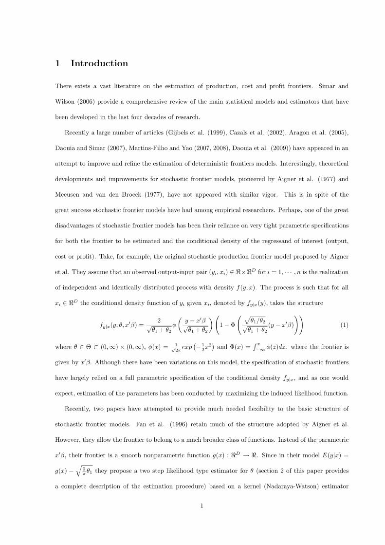
Nonparametric stochastic frontier estimation via profilelikelihood 1

Carlos Martins-Filho

Department of Economics IFPRIUniversity of Colorado 2033 K Street NWBoulder, CO 80309-0256, USA & Washington, DC 20006-1002, USAemail: carlos.martins@colorado.edu email: c.martins-filho@cgiar.orgVoice: + 1 303 492 4599 Voice: + 1 202 862 8144

and

Feng Yao

Department of EconomicsWest Virginia UniversityMorgantown, WV 26505, USAemail: feng.yao@mail.wvu.eduVoice: +1 304 2937867

March, 2010

Abstract. We consider the estimation of a nonparametric stochastic frontier model with composite errordensity which is known up to a finite parameter vector. Our primary interest is on the estimation of theparameter vector, as it provides the basis for estimation of firm specific (in)efficiency. Our frontier modelis similar to that of Fan et al. (1996), but here we extend their work in that: a) we establish the asymp-totic properties of their estimation procedure, and b) propose and establish the asymptotic propertiesof an alternative estimator based on the maximization of a conditional profile likelihood function. Theestimator proposed in Fan et al. (1996) is asymptotically normally distributed but has bias which doesnot vanish as the sample size n → ∞. In contrast, our proposed estimator is asymptotically normallydistributed and correctly centered at the true value of the parameter vector. In addition, our estimatoris shown to be efficient in a broad class of semiparametric estimators. Our estimation procedure providesa fast converging alternative to the recently proposed estimator in Kumbhakar et al. (2007). A MonteCarlo study is performed to shed light on the finite sample properties of these competing estimators.

Keywords and phrases. stochastic frontier models; nonparametric frontiers; profile likelihood estima-tion.

JEL Classifications. C14, C22

1We thank Daniel Henderson, Peter C. B. Phillips and participants in the XX New Zealand Econometrics Study Groupand 2009 Midwest Econometrics Group Meetings for helpful comments.

1 Introduction

There exists a vast literature on the estimation of production, cost and profit frontiers. Simar and

Wilson (2006) provide a comprehensive review of the main statistical models and estimators that have

been developed in the last four decades of research.

Recently a large number of articles (Gijbels et al. (1999), Cazals et al. (2002), Aragon et al. (2005),

Daouia and Simar (2007), Martins-Filho and Yao (2007, 2008), Daouia et al. (2009)) have appeared in an

attempt to improve and refine the estimation of deterministic frontiers models. Interestingly, theoretical

developments and improvements for stochastic frontier models, pioneered by Aigner et al. (1977) and

Meeusen and van den Broeck (1977), have not appeared with similar vigor. This is in spite of the

great success stochastic frontier models have had among empirical researchers. Perhaps, one of the great

disadvantages of stochastic frontier models has been their reliance on very tight parametric specifications

for both the frontier to be estimated and the conditional density of the regressand of interest (output,

cost or profit). Take, for example, the original stochastic production frontier model proposed by Aigner

et al. They assume that an observed output-input pair (yi, xi) ∈ <×<D for i = 1, · · · , n is the realization

of independent and identically distributed process with density f(y, x). The process is such that for all

xi ∈ <D the conditional density function of yi given xi, denoted by fy|x(y), takes the structure

fy|x(y; θ, x′β) =2√

θ1 + θ2

φ

(y − x′β√θ1 + θ2

)(1− Φ

( √θ1/θ2√θ1 + θ2

(y − x′β)

))(1)

where θ ∈ Θ ⊂ (0,∞) × (0,∞), φ(x) = 1√2πexp

(− 1

2x2)

and Φ(x) =∫ x−∞ φ(z)dz. where the frontier is

given by x′β. Although there have been variations on this model, the specification of stochastic frontiers

have largely relied on a full parametric specification of the conditional density fy|x, and as one would

expect, estimation of the parameters has been conducted by maximizing the induced likelihood function.

Recently, two papers have attempted to provide much needed flexibility to the basic structure of

stochastic frontier models. Fan et al. (1996) retain much of the structure adopted by Aigner et al.

However, they allow the frontier to belong to a much broader class of functions. Instead of the parametric

x′β, their frontier is a smooth nonparametric function g(x) : <D → <. Since in their model E(y|x) =

g(x) −√

2π θ1 they propose a two step likelihood type estimator for θ (section 2 of this paper provides

a complete description of the estimation procedure) based on a kernel (Nadaraya-Watson) estimator

1

for E(y|x). Although promising, and intuitive in its construction, the authors did not investigate the

asymptotic properties of their proposed estimator. A brief simulation provided in the paper provides

what seems to be desirable experimental properties, but the results are in their totality rather incomplete.

Perhaps, because of these shortcomings, their model and estimation procedure has not been widely used

by empirical researchers.

More recently, Kumbhabar et al. (2007) take a different approach. Instead of the semiparametric

model proposed by Fan et al. they consider a localized version of Aigner et al. where all “parame-

ters” of the likelihood function depend on x, (g(x), θ1(x), θ2(x)). In this context, they adopt the local

likelihood estimation approach pioneered by Staniswalis (1989) and also explored by Fan et al. (1995).

Although their approach is quite general there is an inconvenience that can potentially be avoided in

a semiparametric model. Specifically, since all “parameters” are local the rate of convergence of their

estimator is rather slow when the number of conditioning variables (inputs, in the case of a production

function) is large. Since it is quite common in frontier models to have a large number of conditioning

variables relative to the sample size, the accuracy of the asymptotic approximations can be rather poor.

For example, in the empirical exercise conducted by Kumbhakar et al., a sample of 500 banks is used

with 9 conditioning variables, calling into question the accuracy of the asymptotic approximation and

the reliability of efficiency rankings.

In this paper we contribute to the stochastic frontier literature in two ways. First, as in Fan et al.

(1996), we consider a semiparametric model. We let the frontier be fully nonparametric (g(x)), but we

consider conditional densities that allow for a parametric expression of the expected value of inefficiency.

A special case of this structure is the model proposed in Fan et al. We study the estimation procedure

proposed by Fan et al in this broader class of models and show that their proposed estimator for the

parameters of the model is consistent. Furthermore, we show that the two stage estimator they propose

is asymptotically normally distributed with parametric convergence rate√n. However, their proposed

estimation procedure produces a bias that does not decay to zero when normalized by√n. In addition,

we show that the variance matrix associated with the asymptotic distribution is not the inverse of the

Fisher information. These results, although new, are not unexpected in light of the work by Stein (1956),

Severini (2000) and Severini and Wong (1992).

2

The second contribution we make in this paper, as it relates to the estimation of stochastic frontiers,

is to define an alternative frontier estimation procedure that is inspired on the procedure described in

Severini and Wong (1992). We show that our proposed estimator is consistent and√n asymptotically

normal. Furthermore, contrary to the procedure proposed by Fan et al., our estimator carries no asymp-

totic bias and is efficient in a class of semiparametric estimators defined in Severini and Wong (1992).1

Although our approach still relies on a partially parametric model, the efficiency estimators we produce

are free from the slow convergence rates described above and no parametric structure is imposed on

the frontier. From a more technical perspective, the main result in this paper is the fact that under

fairly mild conditions local linear regression estimation can be used to estimate least favorable curves in

conditionally parametric models (see Lemma 5 in Severini and Wong (1992)).

Besides this introduction, the paper has five more sections. Section 2 provides a description of our

model and the estimators we study. Section 3 gives the derived asymptotic properties of the estimators

under study and lists a collection of assumptions that are sufficient for the results. A discussion of these

assumptions is also provided. In section 4, a small Monte Carlo study is provided to shed some light on

the finite sample properties of the estimators. The study seems to confirm the results suggested by the

asymptotic theory. Section 5 gives an empirical application using an extensively used data set provided

by Greene (1990). Lastly, section 6 provides a summary and some concluding remarks. All proofs, tables

and graphs are relegated to appendices.

2 A semiparametric stochastic frontier

Let{(

yixi

)}i=1,2,···

be a collection of independent and identically distributed (i.i.d.) random vectors

taking values in <D+1 with yi ∈ < and xi ∈ <D. In the case of production frontiers we take yi to be a

measure of output and xi to be an input vector, but other frontiers (profit, cost) can also be considered

provided that yi is taken to be a scalar. We assume that the density function of(yixi

)exists and

is denoted by f(y, x) when evaluated at(yx

). We denote the marginal density of xi by fx(x) when

evaluated at x. For all x ∈ <D such that fx(x) 6= 0 we denote the conditional density function of yi given

xi by fy|x(y). Throughout, we assume that fy|x(y) belongs to a family of densities which is known up

1See also van der Vaart (1999).

3

to a parameter θ ∈ Θ ⊂ <P , P a positive integer, and a function g(x) : <D → < belonging to a class G.

The true values of θ and g(x) will be denoted by θ0 and g0(x), and our main objective is to estimate θ0

and g0(x) based on a sample χn ={(

yixi

)}ni=1

. We follow Severini and Wong (1992) and assume that

f(y, x) = fy|x(y; θ, g(x))fx(x), i.e., the parameter θ and the function g(x) enter f only through fy|x. This

type of semiparametric structure has been called conditionally parametric models, since conditional on a

particular value x the conditional density is parametrized by a finite number of parameters. In addition,

as a direct link to the stochastic frontier framework, we restrict the class of conditional densities to

those that satisfy E(y|x) ≡ m(x; θ, g) = g(x) − γ(θ) where γ(θ) : Θ → < and V (y|x) = v(θ) where

v(θ) : Θ → (0,∞). Again, for the case of production frontiers, g(x) is interpreted as the systematic

portion of the frontier and γ(θ0) denotes the expected reduction in expected output due to inefficiencies.

It is easy to verify that the conditional density associated with the stochastic frontier model considered

by Aigner et al. (1977) and Fan et al. (1996) is a special case of this structure. Since in their case fy|x is

given by equation (1), then E(y|x) = g(x)− γ(θ) where γ(θ) =√

2π θ1 and V (y|x) = v(θ) = π−2

π θ1 + θ2.

Given this stochastic structure we consider maximum likelihood (ML) type estimators of θ0 and g0(x)

based on the following log-likelihood function

ln(θ, g) =1n

n∑i=1

logfy|x(yi; θ, g(xi)) =1n

n∑i=1

logfy|x(yi; θ,m(xi; θ, g) + γ(θ)). (2)

We investigate two alternative ML procedures. The first, motivated by Fan et al. (1996), is based on

the fact that if g0 were known, a parametric ML estimator for θ0 could be obtained in a routine manner

by maximizing ln(θ, g0) = 1n

∑ni=1 logfy|x(yi; θ,m(xi; θ, g0) + γ(θ)) over the set Θ. Since g0 is unknown,

ln(θ, g0) can be approximated by ln(θ, m+ γ(θ)) = 1n

∑ni=1 logfy|x(yi; θ, m(xi) + γ(θ)) where m(xi) is an

estimator for m(xi; θ, g0). Then, we define the estimator

θ ≡ argmaxθ

ln(θ, m+ γ(θ)). (3)

The second, motivated by Severini and Wong (1992), involves “joint” estimation of θ0 and g0(x).2 To

this end define,

¯n(θ, gx) =

1n

n∑i=1

logfy|x(yi; θ, gx(xi))1hnK

(xi − xhn

)(4)

2For simplicity, but without loss of generality, we will consider throughout the paper the case where D = 1. Although thisdoes impact the rate of convergence of nonparametric estimators in our results, it has no impact on the rate of convergenceof the parametric estimators. Furthermore all results we derive for D = 1 hold, mutatis mutandis, for the case where D > 1.

4

where gx(xi) = α(x) + β(x)(xi − x), K is a kernel function and hn is a bandwidth. The estimation

procedure involves two-steps. First, For fixed x and θ define αθ(x) and βθ(x) as

(αθ(x), βθ(x)) ≡ argmaxα(x),β(x)

¯n(θ, gx). (5)

Second, we define

θ ≡ argmaxθ

ln(θ, αθ) = argmaxθ

1n

n∑i=1

logy|x(yi; θ, αθ(xi)). (6)

The estimator for g0(x) is then given by g(x) ≡ αθ(x). From a computational perspective, the estimators

are fairly easy to implement. In our Monte Carlo study we provide a discussion of bandwidth selection

and the description of an algorithm for obtaining θ. In the next section we study some of the asymptotic

properties for θ and θ.

3 Asymptotic theory

3.1 The estimator θ

We start by listing assumptions that will be used throughout the paper.

Assumption A1. 1. θ0 ∈ int(Θ), where int(Θ) denotes the interior of the compact set Θ ⊂ <P ; 2.

The class G, to which g0 belongs, is given by G = {g(x) : G → H} where G a compact subset of <D,

H a compact subset of <, g(x) ∈ int(H) for all x in G and g(x) is twice continuously differentiable; 3.

E(y|x) ≡ m(x; θ0, g0) = g0(x) − γ(θ0) where γ(θ) : Θ → < which is twice continuously differentiable in

Θ; 4. V (y|x) = v(θ0) where v(θ) : Θ→ (0,∞).

An importance consequence of assumption A1.3 is that, for any θ ∈ Θ, x ∈ G and g ∈ G we have

that g(x) − g0(x) = m(x; θ, g) − m(x; θ, g0). As such, although m(x; θ, g) depends on θ, the difference

|m(x; θ, g)−m(x; θ, g0)| does not.

Assumption A2. 1. fx(x) ∈ [BL, BU ], BL, BU ∈ (0,∞) for all x ∈ G; 2. For all x, s ∈ G we have that

|fx(x)− fx(s)| ≤ C||x− s||E for some C ∈ (0,∞), where ||x||E denotes the Euclidean norm of x.

Since we will be considering kernel based nonparametric estimators, we will make the following stan-

dard assumption on the kernel function K. As in assumption A2, throughout the paper C will represent

an arbitrary positive real number.

Assumption A3. 1. K(φ1, · · · , φD) : SD ⊂ <D → < is a symmetric density function with SD a compact

set; 2.∫φiK(φ1, · · · , φD)d(φ1, · · · , φD) = 0,

∫φiφjK(φ1, · · · , φD)d(φ1, · · · , φD) = σ2

K > 0 if i = j,

5

otherwise µ2 = 0 for all i and j; 3. For all x ∈ SD we have K(x) ≤ C; 4. For all x, s ∈ SD we have

|K(x)−K(s)| ≤ C||x− s||E for some C.

Assumption A3 is satisfied by many commonly used kernels, including Epanechnikov and biweight.

Assumption A4. 1. For all θ ∈ Θ we have that if θ 6= θ0 then fy|x(y; θ, g0(x)) 6= fy|x(y; θ0, g0(x)) for all

(y, x); 2. If {θi}i=1,2,··· is a sequence in Θ such that θi → θ as i→∞, then

logfy|x(y; θi, g0(x))→ logfy|x(y; θ, g0(x)) as i→∞ for all θ ∈ Θ;

3. E(supθ∈Θ

∣∣logfy|x(y; θ, g0(x))∣∣) < ∞; 4. For all (y, x), g ∈ G and θ ∈ Θ, |logfy|x(y; θ, g(x)) −

logfy|x(y; θ, g0(x))| ≤ b(y, x, θ)|g(x) − g0(x)| = b(y, x, θ)|m(x; θ, g) −m(x; θ, g0)| with b(y, x, θ) > 0, and

E (supθ∈Θb(y, x, θ)) <∞.

Assumptions A4.1 and A4.3 guarantee that E(logfy|x(y; θ, g0(x))) has a unique maximum at θ0.

Assumption A5. 1. For all η = g(x) ∈ H, logfy|x(y; θ, η) is twice continuously differentiable with

respect to θ and fy|x(y; θ, η) > 0 on some open ball S0,θ = S(θ0, d(θ0)) of θ0 with S0,θ ⊂ Θ and d(θ0) the

radius of the ball; 2. E(supθ∈S0,θ

∣∣∣ ∂2

∂θj∂θklogfy|x(y; θ, g0(x))

∣∣∣) < ∞ for k, j = 1, · · · , P ; 3. We denote

by ∂∂η the partial derivative operator with respect to the second argument of logfy|x, i.e., η = g(x) and

assume ∂∂η logfy|x(y; θ, g0(x)) is continuously differentiable in S0,θ. Furthermore,∫

supθ∈S0,θ

|| ∂2

∂θ∂ηlogfy|x(y; θ, g0(x))||Efy|x(y; θ0, g0(x))dy <∞

and

E

(supθ∈S0,θ

|| ∂2

∂θ∂ηlogfy|x(y; θ, g0(x))||E |g(2)

0 (x)|

)<∞;

4. The matrix

H = E

(∂2

∂θ∂θ′logfy|x(y; θ0, g0(x))

)+

∂

∂θγ(θ0)E

(∂2

∂θ∂ηlogfy|x(y; θ0, g0(x))

)′+ E

(∂2

∂θ∂ηlogfy|x(y; θ0, g0(x))

)∂

∂θγ(θ0)′

exists and is nonsingular; 5. Let η0 = g0(x) for any x ∈ G and denote by S0,η = S(η0, d(η0)).

logfy|x(y; θ, η) is continuously differentiable on S0,η, an open interval ofH, E

(supη∈S0,η

∣∣∣ ∂∂η logfy|x(y; θ, η)∣∣∣) <

∞ and for all x ∈ G, ∂∂ηE

(logfy|x(y; θ0, g0(x))

)= 0; 6. For all θ ∈ Θ, ∂

∂η logfy|x(y; θ, g0(x)) is continuous

at x,

E

(supθ∈Θ

(∂

∂ηlogfy|x(y; θ, η)

)2)<∞ and E

(supθ∈Θ

(∂

∂ηlogfy|x(y; θ, η)

)2

y2

)<∞.

6

If G is a normed linear space and T (g) : G → < is a functional, we denote the Frechet differential of T

at g with increment h ∈ G of order i = 1, 2 by δiFT (g;h). Note that if the Frechet differentials of order

i = 1, 2 of T exist at g, they coincide with the Gateaux differentials of order i = 1, 2 at g, denoted by

δiGT (g;h) = di

dαT (g + αh) |α=0 (see Luenberger (1969) and Lusternik and Sobolev (1964)). Furthermore,

there exists a Taylor’s Theorem (Graves (1927)) such that we can write,

T (g + h) = T (g) + δ1FT (g;h) +

∫ 1

0

δ2FT (g + th;h)(1− t)dt

= T (g) +dFdgT (g)h+

h2

2

∫ 1

0

d2F

dg2T (g + th)(1− t)dt

where dFdg T (g) and d2F

dg2T (g) are called the first and second order Frechet derivatives of T at g. We take

the norm in G to be supx∈<D |g(x)|.

Assumption A6. 1. logfy|x(y; θ, g0(x)) is twice Frechet differentiable at g0 with increment h(x) =

g(x) − g0(x) and denote the Frechet derivatives of order i = 1, 2 at g0 by diFdgi logfy|x(y; θ, g0(x)); 2.

dFdg logfy|x(y; θ0, g0(x)) is continuous at every x ∈ G; 3. We assume that the matrix

σ2F = E

((∂

∂θlogfy|x(yi; θ0, g0(xi)) + (yi −m(xi; θ0, g0))

∫∂2

∂θ∂ηlogfy|x(y; θ0, g0(xi))fy|x(y)dy

)×

(∂

∂θlogfy|x(yi; θ0, g0(xi)) + (yi −m(xi; θ0, g0))

∫∂2

∂θ∂ηlogfy|x(y; θ0, g0(xi))fy|x(y)dy

)′).

exists and is positive definite.

We observe that Frechet derivatives are, in this case, bounded linear operators from G to <.

Assumption A7. 1. supθ∈S0,θ

∣∣∣E ( ∂∂η logfy|x(y; θ, g0(xi))|xi

)∣∣∣ < ∞; 2. ∂2

∂θi∂ηlogfy|x(y; θ, g0(xi)) is contin-

uously differentiable in S0,θ and E

(supθ∈S0,θ

∣∣∣ ∂3

∂θi∂θj∂ηlogfy|x(y; θ, g0(xi))

∣∣∣ |xi) < ∞ for all xi ∈ G almost

surely; 3. supθ∈S0,θ

∣∣∣E ( ∂2

∂θi∂ηlogfy|x(y; θ, g0(xi))

∣∣∣ |xi) < ∞; 4. E(

∂3

∂θi∂θj∂ηlogfy|x(y; θ, g0(xi))|xi

)is con-

tinuous in S0,θ almost surely; 5. E(|yi − g0(xi)|) < ∞; 6. ∂2

∂θi∂θjE(g

(2)0 (xi) ∂∂η logfy|x(y; θ, g0(xi))

)is

continuous in S0,θ almost surely.

We now define a specific estimator m to be used in equation (3). For any x ∈ G we define m(x) ≡ α(x)

where

(α(x), β(x)) = argminα(x),β(x)

n∑i=1

(yi − α(x)− β(x)(xi − x))2K

(xi − xhn

)(7)

where 0 < hn → 0 as n → ∞ is a bandwidth. This is the local linear estimator of Fan (1992). The

estimator is known to have desirable properties (mini-max efficiency, design-adaptability) and includes

7

the Nadaraya-Watson estimator used in Fan et al. (1996) as a special case. The two theorems establish

the consistency and√n asymptotic normality of θ after suitable centering.

Theorem 1 Given assumptions A1.1-3, A2, A3, A4, and the estimator m(x) defined in (7), if nh3n

log(n) →

∞ as n→∞ then θ − θ0 = op(1).

Theorem 2 Given assumptions A1-A7, and the estimator m(x) defined in (7), if nh3n

log(n) →∞ as n→∞

and hn = O(n−1/5) then√n(θ − θ0 − Bn) d→ N(0, H−1σ2

F H−1), where Bn = −h

2n

2 σ2KH

−1M + op(h2n),

M is a P -vector with pth element given by Mp = E(g

(2)0 (xi) ∂2

∂θp∂ηfy|x(yi; θ0, g0(xi))

), H is as defined in

A5.4 and σ2F is given in A6.3.

Practical use of theorems 1 and 2 requires the verification of assumptions A1.3-4 and A4-A7 for a

chosen conditional density fy|x. Although we have not verified the validity of such assumptions for any

specific class of conditional densities, we have verified that all of these assumptions are met for the density

given in (1).3 Specifically, it is of great practical interest to obtain expressions for σ2F and H. These

expressions allow for the construction of confidence intervals and asymptotically valid hypothesis testing.

Let s2 ≡ θ1 + θ2, λ =√θ1/θ2, w = s

2λs4 , w1 = − 12λ

(θ1+2θ2)θ1θ22s

3 , I =∫ e

√2

sπ3/2

1−erf(e λs√

2)exp(−e2(λ

2

s2 −1

2σ2 ))de,

I1 =∫ e2

√2

sπ3/2

1−erf(e λs√

2)exp(−e2(λ

2

s2 −1

2σ2 ))de, C1 = γ(θ)s4 + λ

swI − (λs )2w√

2π(λ2+1)

s2

λ2+1 + w√

2π(λ2+1) , C2 =

γ(θ)s4 + λ

sw1I−(λs )2w1

√2

π(λ2+1)s2

λ2+1 +w1

√2

π(λ2+1) where erf is the Gaussian error function. If we denote

the (i, j) element of σ2F by σ2

F (i,j), then

σ2F (1,1) =

12s4

+ w2I1 + C21 (s2 − γ(θ)2) +

1s4C1(−3θ2

√θ12/π − (2θ1)3/2(1/

√π) + γ(θ)s2)

− 2wC1

√2

π(λ2 + 1)s2

λ2 + 1

σ2F (1,2) =

12s4

+ ww1I1 + C1C2(s2 − γ(θ)2) + (C1 + C2)(−3θ2

√θ12/π − (2θ1)3/2(1/

√π)

+ γ(θ)s2)− (wC2 + w1C1)

√2

π(λ2 + 1)s2

λ2 + 1

σ2F (2,2) =

12s4

+ w21I1 + C2

2 (s2 − γ(θ)2) +1s4C2(−3θ2

√θ12/π − (2θ1)3/2(1/

√π) + γ(θ)s2)

− 2C2w1

√2

π(λ2 + 1)s2

λ2 + 1

and H =(H11 H12

H21 H22

)where H11 = − 1

2s4 − w2I1 + 2 ∂

∂θ1γ(θ)C1, H12 = − 1

2s4 − ww1I1 + 2 ∂∂θ1

γ(θ)C2,

and H22 = − 12s4 − w

21I1. Given that θ is a consistent estimator for θ0, consistent estimators for σ2

F and

3The verification that all assumptions on the conditional density fy|x are verified for the density described in (1) is givenin Martins-Filho and Yao (2010). There, we also obtain the structure of the matrices which appear in Theorem 2.

8

H can be obtained given the above expression. We note, however, that the integrals in I and I1 must be

numerically evaluated.

It is not surprising that in theorem 2 a parametric estimator - θ - that is based on averages of

a nonparametrically estimated curve converges at a parametric√n rate (see Doksum and Samarov

(1995)). Additionally, theorem 2 shows that θ carries an asymptotic bias that does not decay to zero

when normalized by√n. The presence of this bias is precisely the motivation for the generalized profile

likelihood estimator proposed by Severini and Wong (1992) for conditionally parametric models. Hence,

we now turn our attention to the estimator θ.

3.2 The estimator θ

Suppose we consider a reparametrization of fy|x(y; θ, g(x)) given by fy|x(y; θ, αθ(x)), where for every

x ∈ G, αθ(x) : Θ→ H with αθ0(x) = g0(x). The parametric submodel described by the curve αθ(x) has

Fisher information given by

I0

(∂

∂θαθ0(x)

)= E

(∂

∂θlogfy|x(y; θ0, g0(x)) +

dFdglogfy|x(y; θ0, g0(x))

∂

∂θαθ0(x)

)(∂

∂θlogfy|x(y; θ0, g0(x))

+dFdglogfy|x(y; θ0, g0(x))

∂

∂θαθ0(x)

)′where ∂

∂θαθ0(x) is the tangent vector associated with αθ(x) evaluated at θ0. As argued in van der Vaart

(1999), it is desirable to minimize the information associated with the parametric submodel induced by

αθ(x). Since the information depends only on the tangent vector it is natural to define4

Iθ0 = inf∂∂θαθ0 (x)

I0

(∂

∂θαθ0(x)

). (8)

Bickel et al. (1993) show that provided E((dFdg logfy|x(y; θ0, g0(x))2|x) > 0 the minimizer for (8), say

∂∂θαθ0(x)∗, satisfies

∂

∂θkαθ0(x)∗ = −

E(

∂∂θk

logfy|x(y; θ0, g0(x))dFdg logfy|x(y; θ0, g0(x))|x)

E((dFdg logfy|x(y; θ0, g0(x))2|x)for k = 1, · · · , P. (9)

The tangent vector ∂∂θαθ0(x)∗ is called a least favorable direction. Interestingly, if we let αθ(x) ∈ G be the

unique maximizer of E(logfy|x(y; θ, g(x))|x) for fixed x and θ, using a Taylor’s expansion around θ0 shows

that αθ(x) minimizes Fisher’s information, provided E(logfy|x(y; θ, g(x))|x) < E(logfy|x(y; θ0, g0(x))|x)

4We follow the usual practice of defining, for any two squared matrices A and B, A ≤ B if, and only if, B−A is positivesemidefinite.

9

whenever θ 6= θ0. As such, Severini and Wong define a least favorable curve for a conditional parametric

model as αθ(x) : Θ→ H that for every x ∈ G satisfies the following: (1) For each x ∈ G, αθ0(x) = g0(x);

(2) For each x ∈ G, ∂∂θαθ(x) and ∂2

∂θ∂θ′αθ(x) exist and supx∈G| ∂∂θpαθ(x)| < ∞, and sup

x∈G| ∂2

∂θp∂θmαθ(x)| < ∞

for all m, p = 1, ..., P ; (3) For each x ∈ G, ∂∂θαθ0(x) minimizes the Fisher information for the parametric

sub-model described by logfy|x(y; θ, αθ(x)).

Now, consider an arbitrary estimator for αθ(x) given by αθ(x) and define

θ ≡ argmaxθ

ln(θ, αθ) = argmaxθ

1n

n∑i=1

logy|x(yi; θ, αθ(xi)). (10)

The following theorem establishes the asymptotic normality and consistency of θ conditional on the

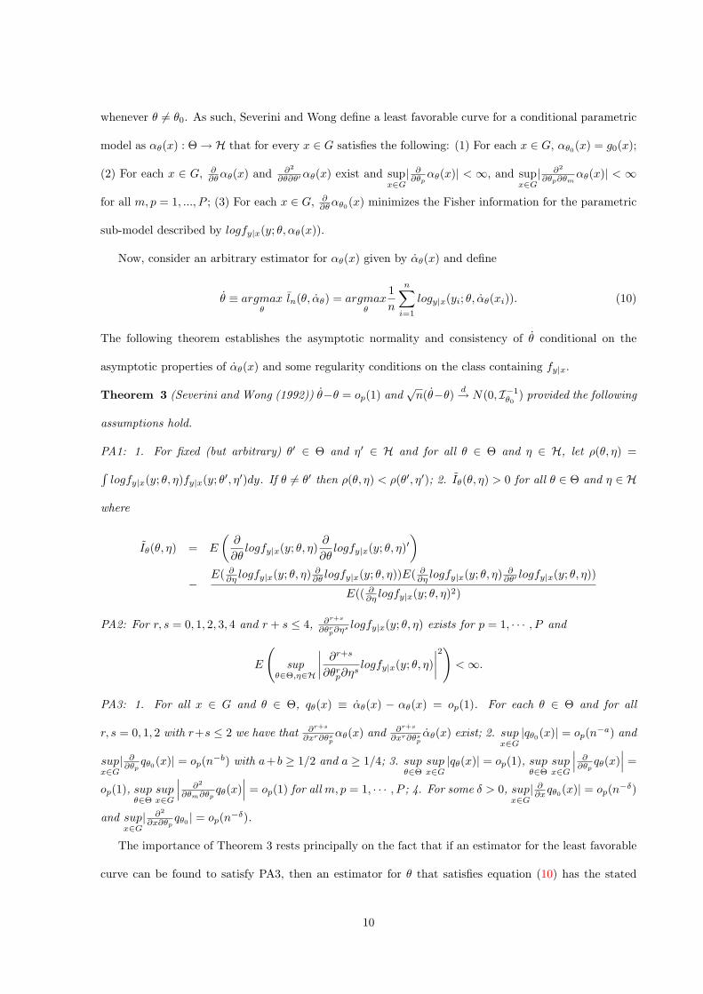
asymptotic properties of αθ(x) and some regularity conditions on the class containing fy|x.

Theorem 3 (Severini and Wong (1992)) θ−θ = op(1) and√n(θ−θ) d→ N(0, I−1

θ0) provided the following

assumptions hold.

PA1: 1. For fixed (but arbitrary) θ′ ∈ Θ and η′ ∈ H and for all θ ∈ Θ and η ∈ H, let ρ(θ, η) =∫logfy|x(y; θ, η)fy|x(y; θ′, η′)dy. If θ 6= θ′ then ρ(θ, η) < ρ(θ′, η′); 2. Iθ(θ, η) > 0 for all θ ∈ Θ and η ∈ H

where

Iθ(θ, η) = E

(∂

∂θlogfy|x(y; θ, η)

∂

∂θlogfy|x(y; θ, η)′

)−

E( ∂∂η logfy|x(y; θ, η) ∂∂θ logfy|x(y; θ, η))E( ∂∂η logfy|x(y; θ, η) ∂∂θ′ logfy|x(y; θ, η))

E(( ∂∂η logfy|x(y; θ, η)2)

PA2: For r, s = 0, 1, 2, 3, 4 and r + s ≤ 4, ∂r+s

∂θrp∂ηs logfy|x(y; θ, η) exists for p = 1, · · · , P and

E

(sup

θ∈Θ,η∈H

∣∣∣∣ ∂r+s∂θrp∂ηslogfy|x(y; θ, η)

∣∣∣∣2)<∞.

PA3: 1. For all x ∈ G and θ ∈ Θ, qθ(x) ≡ αθ(x) − αθ(x) = op(1). For each θ ∈ Θ and for all

r, s = 0, 1, 2 with r+s ≤ 2 we have that ∂r+s

∂xr∂θspαθ(x) and ∂r+s

∂xr∂θspαθ(x) exist; 2. sup

x∈G|qθ0(x)| = op(n−a) and

supx∈G| ∂∂θp qθ0(x)| = op(n−b) with a+ b ≥ 1/2 and a ≥ 1/4; 3. sup

θ∈Θsupx∈G|qθ(x)| = op(1), sup

θ∈Θsupx∈G

∣∣∣ ∂∂θp qθ(x)∣∣∣ =

op(1), supθ∈Θ

supx∈G

∣∣∣ ∂2

∂θm∂θpqθ(x)

∣∣∣ = op(1) for all m, p = 1, · · · , P ; 4. For some δ > 0, supx∈G| ∂∂xqθ0(x)| = op(n−δ)

and supx∈G| ∂2

∂x∂θpqθ0 | = op(n−δ).

The importance of Theorem 3 rests principally on the fact that if an estimator for the least favorable

curve can be found to satisfy PA3, then an estimator for θ that satisfies equation (10) has the stated

10

asymptotic properties. In contrast with the estimator described in Theorem 2, θ is not biased asymp-

totically and is efficient in the sense that it is based on a suitable estimator αθ(x) for the least favorable

curve.

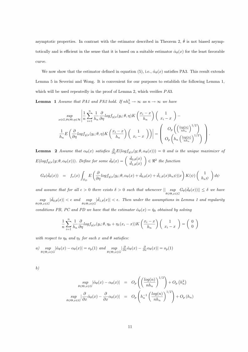
We now show that the estimator defined in equation (5), i.e., αθ(x) satisfies PA3. This result extends

Lemma 5 in Severini and Wong. It is convenient for our purposes to establish the following Lemma 1,

which will be used repeatedly in the proof of Lemma 2, which verifies PA3.

Lemma 1 Assume that PA1 and PA2 hold. If nh3n →∞ as n→∞ we have

supx∈G,θ∈Θ,η∈H

∣∣∣∣∣ 1nn∑i=1

1hn

∂

∂ηlogfy|x(yi; θ, η)K

(xi − xhn

)(1

xi − x

)−

1hnE

(∂

∂ηlogfy|x(yi; θ, η)K

(xi − xhn

)(1

xi − x

))∣∣∣∣ =

Op

((log(n)nhn

)1/2)

Op

(hn

(log(n)nhn

)1/2) .

Lemma 2 Assume that αθ(x) satisfies ∂∂ηE(logfy|x(y; θ, αθ(x))) = 0 and is the unique maximizer of

E(logfy|x(y; θ, αθ(x))). Define for some dθ(x) =(d0,θ(x)d1,θ(x)

)∈ <2 the function

Gθ(dθ(x)) = fx(x)∫SD

E

(∂

∂ηlogfy|x(yi; θ, αθ(x) + d0,θ(x) + d1,θ(x)hnψ)|x

)K(ψ)

(1

hnψ

)dψ

and assume that for all ε > 0 there exists δ > 0 such that whenever || supθ∈Θ,x∈G

Gθ(dθ(x))|| ≤ δ we have

supθ∈Θ,x∈G

|d0,θ(x)| < ε and supθ∈Θ,x∈G

|d1,θ(x)| < ε. Then under the assumptions in Lemma 1 and regularity

conditions PB, PC and PD we have that the estimator αθ(x) = η0 obtained by solving

1n

n∑i=1

1hn

∂

∂ηlogfy|x(yi; θ, η0 + η1(xi − x))K

(xi − xhn

)(1

xi − x

)=(

00

)

with respect to η0 and η1 for each x and θ satisfies:

a) supθ∈Θ,x∈G

|αθ(x)− αθ(x)| = op(1) and supθ∈Θ,x∈G

| ∂∂x αθ(x)− ∂∂xαθ(x)| = op(1)

b)

supθ∈Θ,x∈G

|αθ(x)− αθ(x)| = Op

((log(n)nhn

)1/2)

+Op(h2n

)sup

θ∈Θ,x∈G| ∂∂xαθ(x)− ∂

∂xαθ(x)| = Op

(h−1n

(log(n)nhn

)1/2)

+Op (hn)

11

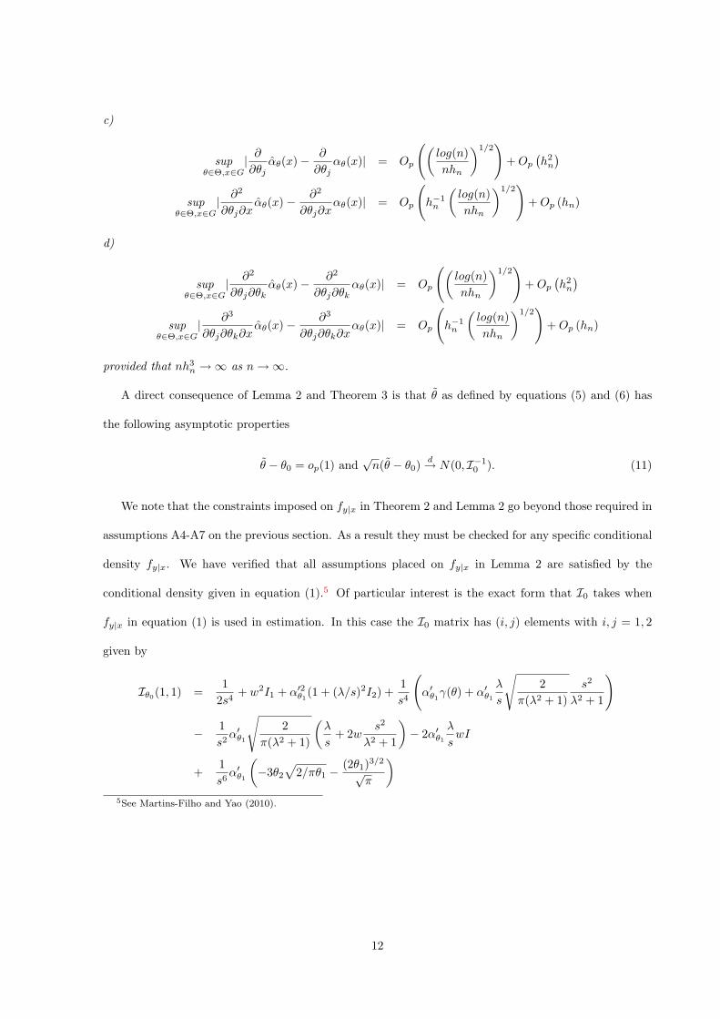
c)

supθ∈Θ,x∈G

| ∂∂θj

αθ(x)− ∂

∂θjαθ(x)| = Op

((log(n)nhn

)1/2)

+Op(h2n

)sup

θ∈Θ,x∈G| ∂2

∂θj∂xαθ(x)− ∂2

∂θj∂xαθ(x)| = Op

(h−1n

(log(n)nhn

)1/2)

+Op (hn)

d)

supθ∈Θ,x∈G

| ∂2

∂θj∂θkαθ(x)− ∂2

∂θj∂θkαθ(x)| = Op

((log(n)nhn

)1/2)

+Op(h2n

)sup

θ∈Θ,x∈G| ∂3

∂θj∂θk∂xαθ(x)− ∂3

∂θj∂θk∂xαθ(x)| = Op

(h−1n

(log(n)nhn

)1/2)

+Op (hn)

provided that nh3n →∞ as n→∞.

A direct consequence of Lemma 2 and Theorem 3 is that θ as defined by equations (5) and (6) has

the following asymptotic properties

θ − θ0 = op(1) and√n(θ − θ0) d→ N(0, I−1

0 ). (11)

We note that the constraints imposed on fy|x in Theorem 2 and Lemma 2 go beyond those required in

assumptions A4-A7 on the previous section. As a result they must be checked for any specific conditional

density fy|x. We have verified that all assumptions placed on fy|x in Lemma 2 are satisfied by the

conditional density given in equation (1).5 Of particular interest is the exact form that I0 takes when

fy|x in equation (1) is used in estimation. In this case the I0 matrix has (i, j) elements with i, j = 1, 2

given by

Iθ0(1, 1) =1

2s4+ w2I1 + α′2θ1(1 + (λ/s)2I2) +

1s4

(α′θ1γ(θ) + α′θ1

λ

s

√2

π(λ2 + 1)s2

λ2 + 1

)

− 1s2α′θ1

√2

π(λ2 + 1)

(λ

s+ 2w

s2

λ2 + 1

)− 2α′θ1

λ

swI

+1s6α′θ1

(−3θ2

√2/πθ1 −

(2θ1)3/2

√π

)5See Martins-Filho and Yao (2010).

12

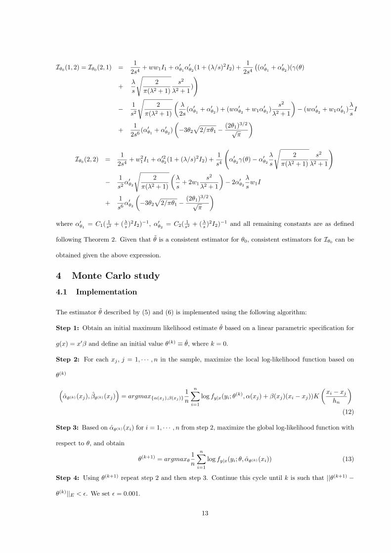
Iθ0(1, 2) = Iθ0(2, 1) =1

2s4+ ww1I1 + α′θ1α

′θ2(1 + (λ/s)2I2) +

12s4

((α′θ1 + α′θ2)(γ(θ)

+λ

s

√2

π(λ2 + 1)s2

λ2 + 1)

)

− 1s2

√2

π(λ2 + 1)

(λ

2s(α′θ1 + α′θ2) + (wα′θ2 + w1α

′θ1)

s2

λ2 + 1

)− (wα′θ2 + w1α

′θ1)

λ

sI

+1

2s6(α′θ1 + α′θ2)

(−3θ2

√2/πθ1 −

(2θ1)3/2

√π

)

Iθ0(2, 2) =1

2s4+ w2

1I1 + α′2θ2(1 + (λ/s)2I2) +1s4

(α′θ2γ(θ)− α′θ2

λ

s

√2

π(λ2 + 1)s2

λ2 + 1

)

− 1s2α′θ2

√2

π(λ2 + 1)

(λ

s+ 2w1

s2

λ2 + 1

)− 2α′θ2

λ

sw1I

+1s6α′θ2

(−3θ2

√2/πθ1 −

(2θ1)3/2

√π

)where α′θ1 = C1( 1

s2 + (λs )2I2)−1, α′θ2 = C2( 1s2 + (λs )2I2)−1 and all remaining constants are as defined

following Theorem 2. Given that θ is a consistent estimator for θ0, consistent estimators for Iθ0 can be

obtained given the above expression.

4 Monte Carlo study

4.1 Implementation

The estimator θ described by (5) and (6) is implemented using the following algorithm:

Step 1: Obtain an initial maximum likelihood estimate θ based on a linear parametric specification for

g(x) = x′β and define an initial value θ(k) ≡ θ, where k = 0.

Step 2: For each xj , j = 1, · · · , n in the sample, maximize the local log-likelihood function based on

θ(k)

(αθ(k)(xj), βθ(k)(xj)

)= argmax{α(xj),β(xj)}

1n

n∑i=1

log fy|x(yi; θ(k), α(xj) + β(xj)(xi − xj))K(xi − xjhn

)(12)

Step 3: Based on αθ(k)(xi) for i = 1, · · · , n from step 2, maximize the global log-likelihood function with

respect to θ, and obtain

θ(k+1) = argmaxθ1n

n∑i=1

log fy|x(yi; θ, αθ(k)(xi)) (13)

Step 4: Using θ(k+1) repeat step 2 and then step 3. Continue this cycle until k is such that ||θ(k+1) −

θ(k)||E < ε. We set ε = 0.001.

13

Step 5: Fix the estimator θ at the value obtained from the last cycle of step 4 and put g(x) = αθ(x) in

step 2.

As pointed out by Lam and Fan (2008), this algorithm is equivalent to a Newton-Raphson procedure

but (13) incorporates the functional dependence of αθ(x) on θ by using the value of θ(k) from the previous

step as a proxy for θ. Specifically, the algorithm treats the ddθ gθ(x) and d2

dθdθ′ gθ(x) in the Newton-Raphson

procedure as zeros and computes gθ(x) using the values of θ(k) in the previous iteration. Thus the

maximization is easier to carry out. We recommend calculating (gθ(k)(x),∂gθ(k)

(x)

∂x ) in step 2 at a fixed

but fine grid of points of x. Then use linear interpolation to calculate the other values of gθ(k)(x).

Implementation of our estimator requires the selection of a bandwidth hn. Since g0(x) = E(y|x)+γ(θ0)

where γ(θ) is a non-stochastic function of θ, we use the data driven rule-of-thumb bandwidth hROT of

Ruppert et al. (1995). We observe that hROT /h∗n− 1 = op(1) where h∗n is the bandwidth that minimizes

the local linear regression estimator’s asymptotic mean squared error (AMISE). Since, h∗n = O(n−15 ) we

have that h∗n → 0 at a speed that is consistent with that required by the asymptotic theory.

4.2 Data Generation and Results

In this section, we perform a Monte Carlo study which implements our profile likelihood semi-parametric

stochastic frontier estimator and provides evidence on its finite sample performance. We consider the

stochastic production frontier model of Fan et al. (1996) where output-input pairs (yi, xi) are gener-

ated in accordance with assumptions A1, A2 and the conditional density given by (1). We consider

four different functional forms for g(x): g1(x) = 1 + x, g2(x) = 1 + ln(1 + x), g3(x) = 1 − 11+x and

g4(x) = 1 + 0.5arctan(20(x − 0.5)). The first three functions are considered in Fan et al. (1996) and

we introduce the last one, which exhibits more pronounced nonlinearity. We generate the univariate

input xi from an uniform distribution on [0, 1]. To facilitate comparison, the parameter θ is set at

θ(1) = (1.379, 0.501), θ(2) = (0.988, 0.642) and θ(3) = (0.551, 0.799) to coincide with the values consid-

ered by Aigner et al. (1977) and Fan et al. (1996). Note that the ratio ( θ1θ2 ) decreases from θ(1) to

θ(3). Figure 1 provides a plot of a typical simulated sample for the production frontier g1(x), and Fig-

ure 2 provides a similar plot for the production frontier g4(x), where both samples were generated with

(θ1, θ2) = (1.379, 0.501). Superimposed on the plot are the true production frontier, estimated frontiers

14

with both a profile likelihood (PL) estimator (θ) and a plug in (PI) estimator (θ). These figures suggest

that both estimators seem to capture fairly well the shape of the underlying production frontier.

The PL estimator is implemented using the algorithm described above and the bandwidth hROT . We

use the Epanechnikov kernel in the estimation, which satisfies assumption A3. For comparison purpose

we also include in the study the PI estimator and a parametric maximum likelihood (ML) estimator

constructed under the correct specification of the production frontier. The parametric ML estimator

is, under these circumstances, expected to outperform the PL and PI estimators. The PI estimator is

implemented as described by Fan et al. (1996), but here the conditional expectation m0(x) is estimated

via a local linear estimator, so that the asymptotic characterization given in section 3 is applicable. We set

the sample sizes at n = 300, 600 and 900, and perform 500 replications for each experimental design. We

investigate the performances of PL, PI and ML in estimating the global parameter θ. The performance

of the estimators is summarized by their bias, standard deviation and root mean squared error, which

are provided in Tables 1-4.

As suggested by the asymptotic theory, the performance of all three estimators in terms of bias,

standard deviation, and root mean squared error generally improves as n increases, with a few exceptions

for the bias. All three estimators generally exhibit a negative bias in estimating θ1 and a positive bias in

estimating θ2 with a few exceptions for small samples when (θ1, θ2) = (0.551, 0.799). It is also clear that

it is harder to estimate θ1 than to estimate θ2, as the bias, standard deviation and root mean squared

error for all estimators of θ2 are smaller than those of θ1. The above observations are consistent with

the results in the Monte Carlo studies of Fan et al. (1996) and Aigner et al. (1977). General conclusions

regarding the relative performance of the estimators are unambiguous and conform with our expectations.

The parametric ML estimator performs best since it is based on a correct specification of the production

frontier and the distribution of the composite error term. Among the two semiparametric estimators that

relax the parametric assumption on the production frontier, the PL estimator we propose outperforms the

PI estimator of Fan et al. across almost all experimental designs, and the improvement is significant. For

example, in the simulation with g1(x) as production frontier and (θ1, θ2) = (1.379, 0.501), the reduction

in the root mean squared error from the PL estimator over that of the PI estimator are about 5% in

estimating both θ1 and θ2. A few exceptions occur for the smallest sample when (θ1, θ2) = (0.551, 0.799),

15

which corresponds to the case where the variance of the efficiency term (π−2π θ1) is significantly smaller

than that of the noise in the production frontier (θ2). The result is generally consistent with the fact

that asymptotically the PL estimator reaches a semiparametric efficiency bound, while PI does not.

To provide further evidence of the finite sample performance of the PL and PI estimators, we provide

the associated Rosenblatt density estimates for θ1 in Figure 3 and for θ2 in Figure 4, centered around

the true value (θ1, θ2) = (1.379, 0.501) based on 500 simulations of sample size n = 300 and 900 for the

convex production technology g3(x). Other experimental designs provide similar graphs. As indicated in

these figures, the estimated densities for both PI and PL get taller and possess more pronounced peaks

as the sample size increases, confirming the asymptotic results. Furthermore, the kernel density for our

estimates is relatively taller and more tightly centered around zero than that for Fan et al. estimates,

indicating smaller bias and variance for our estimates. Overall our simulations seem to indicate that our

proposed estimator can outperform the estimator proposed by Fan et al. (1996) in finite samples.

5 An empirical application

In this section we provide an empirical application of the semiparametric profile likelihood estimation

(PL) using data on the U.S. electricity industry. The data have been used by Christensen and Green

(1976), Gijbels et al. (1999), Martins-Filho and Yao (2008) and are provided in Green (1990). The model

fitted in Green (1990) is a restricted specification of the cost function,

Ln(Cost/Pf ) = β0 + β1LnQ+ β2Ln2Q+ β3Ln(Pl/Pf ) + β4Ln(Pk/Pf ) + ε. (14)

The output (Q) is a function of three factors, labor (l), capital (k), and fuel (f). The three factor prices

are Pl, Pk, and Pf . The restriction of linear homogeneity in the factor price has been imposed on the

cost function. For detailed description of the data set and analysis, see Christensen and Greene (1976)

and Greene(1990). Since we estimate a cost frontier rather than a production frontier, equation (1) is

slightly modified and written as

fy|x(y; θ1, θ2, g(x)) =2√

θ1 + θ2

φ

(y − g(x)√θ1 + θ2

)(1− Φ

(−√θ1/θ2√θ1 + θ2

(y − g(x))

)).

Since the parametric specification of the cost frontier might be restrictive, we utilize a semiparametric PL

16

approach to estimate the frontier and analyze the efficiency levels of firms in the electric utility industry.

We implement the PL estimator as described in section 4 using a gaussian product kernel and a bandwidth

given by hl = cσxln− 1

4+p with l = 1, 2, 3 (see Hardle (1990) and Fan et al. (1996)), where c is a constant set

to be 1.25, and σxl is the sample standard deviation of xl, x1 = LnQ, x2 = Ln(Pl/Pf ), x3 = Ln(Pk/Pf ).

We note that the assumption of compact support for the kernel (A3) is made to facilitate the proof, but

our asymptotic results continue to hold with a gaussian kernel. The estimation results give θ1 = 0.0010,

θ2 = 0.0103 with ˆtheta1 accounting for only 3.37% of the estimated conditional variance of Ln(Cost/Pf ).

In contrast, as provided in Greene (1990) where the linear cost frontier and normal half-normal composite

error model is fitted with maximum likelihood estimation (ML), the estimation results give θ1 = 0.0241,

θ2 = 0.0115 with θ1 accounting for 43.2% of the estimated conditional variance of Ln(Cost/Pf ). The

changes in the estimated parameters and changes in the allocation of total variance of the disturbance

to the inefficiency term, similar in the direction but smaller in magnitude, are also observed in Fan et

al. for Quebec dairy farm data and Green (1990) for gamma-distributed frontier model. Relatively small

estimates of the one-sided components of the disturbance are also obtained in the empirical examples in

Aigner et al. We observe that the semiparametric estimation gives estimation results quite different from

the parametric approach, suggesting that the cost frontier may be nonlinear in xl.

We plot the cost frontier estimated by both PL and ML against the observed cost in Figure 5. The PL

estimates seem to be slightly more concentrated around the line of equality between estimated frontier

and observed cost than the ML estimates, although we do not observe a substantial difference between

the quality of fit using the two approaches. To compare the difference in the two estimates, we provide the

plot of estimated marginal cost against the output in Figure 6. The ML procedure assumes a parametric

frontier that implies a marginal cost given by β1 + 2β2LnQ. We obtain the marginal cost of PL by

maximizing the local likelihood function in equation (12) at different sample values of Ln(Q) with θ1

and θ2 reported above, fixing Ln(Pl/Pf ) and Ln(Pk/Pf ) at the sample mean values. The marginal costs

differ substantially over the range of Ln(Q), indicating that the assumption that marginal cost is linear

in Ln(Q) might be too restrictive.

Based on the frontier estimation results, we evaluate firm specific efficiency levels. We follow Jondrow

et al. (1982) and obtain firm-specific efficiency as

17

efi =(θ1 + θ2)

12√θ1/θ2

1 + θ1/θ2

φ(−√θ1/θ2√θ1+θ2

ε)

1− Φ(−√θ1/θ2√θ1+θ2

ε)+

√θ1/θ2√θ1 + θ2

ε

.The unknown parameters are replaced with their estimates and ε is replaced with εi = yi − g(xi). Since

the data are presented in logs, the efficiencies are calculated as exp(efi ). The estimated efficiencies with

PL are summarized with a Rosenblatt density plot in Figure 7. Estimated efficiencies fall between 1.0171

and 1.0370 and the average efficiency score is 1.0251. Thus, on average, cost of the U.S. electricity

utility industry is increased by 2.5% due to inefficiency. The average efficiency score is roughly the same

as that obtained in a COLS/gamma estimate provided in Table 2 of Green (1990). In contrast, the

estimated efficiencies with ML range from 1.0308 to 1.4794 with an average efficiency score of 1.1338.

The difference is further illustrated in Figure 8, the plot of the estimated efficiencies with both PL and ML

against the observed cost. It seems that ML predicts much higher inefficiencies than the semiparametric

PL approach. This is consistent with the observations made in Kumbhakar et al. (2007) using a local

maximum likelihood approach. The high estimated inefficiency might attributed to a misspecification of

the frontier function.

6 Summary and conclusions

In this paper we consider the estimation of a semiparametric stochastic frontier model. We study two

estimators for the parameters of the model. We first establish the asymptotic properties (until now

unknown) of an estimator proposed by Fan et al. (1996). The estimator is shown to be consistent and

asymptotically normal, however the asymptotic distribution is incorrectly centered. We then propose a

new estimator based on a profile likelihood procedure for conditionally parametric models first suggested

by Severini and Wong (1992). We show that our estimator is consistent, asymptotically normal and

efficient in a suitably defined class of semiparametric estimators. Practical use of the estimators requires

the specification of a conditional density that must meet some regularity conditions. We verify that the

density used in Aigner et al. (1977) and Fan et al. (1996) satisfy all of the stated regularity conditions.

However, future work should investigate whether broader classes of densities that may potentially be used

by applied researchers in efficiency and productivity studies meet such regularity conditions.

18

Appendix 1 - Assumptions and proofs

Assumption PB: 1. supx∈G

fx(x) < C; 2. supx∈G

f(1)x (x) < C; 3. sup

x∈Gf

(2)x (x) < C; 4. inf

x∈Gfx(x) > 0; 5.

supx∈G,θ∈Θ

| ∂∂xαθ(x)| < C.

Assumption PC:∫supx∈G

∣∣∣ ∂∂x ( ∂s1+s2+r

∂θs1k ∂θ

s2j ∂ηr

logfy|x(y; θ, αθ(x))fy|x(y; θ, g0(x)))∣∣∣ dy < c, with s1, s2, r ≥ 0, where (s1, s2, r) =

(0, 0, 1), (1, 0, 1), (0, 1, 1), (1, 1, 1).

Assumption PD:

supx∈G,θ∈Θ,η∈H

∣∣∣∫ ∂s1+s2+r

∂θs1k ∂θ

s2j ∂ηr

logfy|x(y; θ, η) ∂j

∂xj fy|x(y; θ0, g0(x))dy∣∣∣ < C with s1, s2, r ≥ 0, for j=0, s1 + s2 +

r ≤ 4, and (s1, s2, r) = (0,0,5); for j=1, (s1, s2, r) = (0,0,1), (1,0,2), (0,1,2), (1,0,3), (0,1,3), (0,0,4),

(0,0,3), (1,1,2), (1,1,3), (0,1,4), (1,0,4), (0,0,5) and for j=2, (s1, s2, r) = (0,0,1), (0,0,2), (0,0,3), (1,0,1),

(0,1,1), (1,0,2), (0,1,2), (1,0,3), (0,1,3), (0,0,4), (1,1,1), (1,1,2), (1,1,3), (0,1,4), (1,0,4), (0,0,5).

Theorem 1: Proof. Given A1.1-3, A4 and the definition of θ, by Theorem 2.1 in Newey and McFadden

(1994) it suffices to prove that supθ∈Θ

∣∣ln(θ, m+ γ(θ))− E(ln(θ, g0)

)∣∣ = op(1). We do so by establishing

that supθ∈Θ

∣∣ln(θ, m+ γ(θ))− ln(θ, g0)∣∣ = op(1) and supθ∈Θ

∣∣ln(θ, g0)− E(ln(θ, g0)

)∣∣ = op(1). First,

note that by A1.3 and A4.4 supθ∈Θ

∣∣ln(θ, m+ γ(θ))− ln(θ, g0)∣∣ ≤ 1

n

∑ni=1 supθ∈Θb(yi, xi, θ)|m(xi) −

m(xi; θ, g0)|. If nh3n

log(n) → ∞ as n → ∞ and given A2.2 and A3, for a compact set G, we have

supx∈G|m(x)−m(x; θ, g0)| = op(1) (Martins-Filho and Yao, 2007). Given that E (supθ∈Θb(yi, xi, θ)) <∞

and the fact that (yi, xi) are i.i.d, we conclude that supθ∈Θ

∣∣ln(θ, m+ γ(θ))− ln(θ, g0)∣∣ = op(1). Second,

note that

∣∣ln(θ, g0)− E(ln(θ, g0)

)∣∣ ≤ 1n

n∑i=1

∣∣logfy|x(yi; θ, g0(xi))− E(logfy|x(yi; θ, g0(xi))

)∣∣ .By the Heine-Borel theorem every open covering of Θ contains a finite subcover {Sk}Kk=1 where Sk =

S(θk, d(θk)) denotes an open sphere centered at θk with radius d(θk) > 0. Now let

µ(yi, xi, θ, g0, d(θ)) = supθ′∈S(θ,d(θ))

∣∣logfy|x(yi; θ, g0(xi))− logfy|x(yi; θ′, g0(xi))∣∣ .

By A4.2 µ(yi, xi, θ, g0, d(θ)) → 0 for all θ ∈ Θ as d(θ) → 0 almost everywhere arcording to f(y, x).

By the triangle inequality µ(yi, xi, θ, g0, d(θ)) ≤ 2supθ∈Θ|logfy|x(yi; θ, g0(xi))|. By A4.3 and Lebesgue’s

dominate convergence theorem (LDC) we conclude that for any ε, d > 0, E (µ(yi, xi, θ, g0, d(θ))) < ε

19

whenever d(θ) < d. Letting d(θk) < d for all k = 1, ...,K we have E(µ(yi, xi, θk, g0, d(θk))) < ε for all

k. Also,∣∣E(logfy|x(yi; θ, g0(xi))− E(logfy|x(yi; θk, g0(xi))

∣∣ ≤ E (µ(yi, xi, θk, g0, d(θk))) < ε. Hence, for

θ ∈ Sk we have

∣∣ln(θ, g0)− E(ln(θ, g0)

)∣∣ ≤ n−1n∑i=1

(µ(yi, xi, θk, g0, d(θk))− E(µ(yi, xi, θk, g0, d(θk))))

+

∣∣∣∣∣n−1n∑i=1

(logfy|x(yi; θk, g0(xi))− E(logfy|x(yi; θk, g0(xi))

)∣∣∣∣∣+ 2ε

Since E(µ(yi, xi, θk, g0, d(θk))) < ∞ and E(|logfy|x(yi; θk, g0(xi))|) < ∞, we have, by the strong law of

large numbers, that there exists Nε,k such that n > Nε,k gives∣∣∣∣∣n−1n∑i=1

µ(yi, xi, θk, g0, d(θk))− E (µ(yi, xi, θk, g0, d(θ)))

∣∣∣∣∣ < ε

and n−1∑ni=1

∣∣logfy|x(yi; θk, g0(xi))− E(logfy|x(yi; θk, g0(xi)))∣∣ < ε. Given that K is finite, for all n >

maxkNk,ε we have supθ∈Θ|ln(θ, g0)− E(ln(θ, g0))| = op(1).

Theorem 2: Proof. Given A6.1 and Taylor’s Theorem in Graves (1927),

ln(θ, m+ γ(θ)) =1n

n∑i=1

logfy|x(yi; θ, g0(xi)) +1n

n∑i=1

dFdglogfy|x(yi, θ, g0(xi))(m(xi)−m(xi; θ, g0))

+1

2n

n∑i=1

(m(xi)−m(xi; θ, g0))2

∫ 1

0

d2F

dg2logfy|x(yi; θ, g0(xi) + t(m(xi)−m(xi; θ, g0))

× (1− t)dt.

Denoting the last term in the above inequality by cn and given that dFdg is a bounded linear functional

from G to <, we have

|cn| ≤1

2n

n∑i=1

(supx∈G|m(x)−m(x; θ, g0)|

)2 ∫ 1

0

C supx∈G|g0(x) + t(m(x)−m(x; θ, g0))|(1− t)dt

≤ 12

(supx∈G|m(x)−m(x; θ, g0)|

)2 ∫ 1

0

C

(supx∈G|g0(x)|+ t sup

x∈G|(m(x)−m(x; θ, g0))|

)(1− t)dt

≤ C

((supx∈G|m(x)−m(x; θ, g0)|

)2

+(

supx∈G|m(x)−m(x; θ, g0)|

)3).

Since supx∈G|m(x) −m(x; θ, g0)| = Op

((log(n)nhn

)1/2

+ h2n

), it follows that if hn = O(n−1/5) we have that

|cn| = op(n−1/2). Consequently, we can write

ln(θ, m+ γ(θ)) = ln(θ, g0(xi)) +1n

n∑i=1

dFdglogfy|x(yi, θ, g0(xi))(m(xi)−m(xi; θ, g0)) + op(n−1/2).

20

Since ∂∂θ ln(θ, m+γ(θ)) = 0 we have . By A5.1 and the mean value theorem there exists some θ ∈ L(θ, θ0)

(the line segment uniting θ and θ0) such that

− ∂2

∂θ∂θ′ln(θ, m+ γ(θ))

√n(θ − θ0) =

√n∂

∂θln(θ0, m+ γ(θ0)). (15)

We now write

√n∂

∂θln(θ0, m+ γ(θ0)) =

√n∂

∂θln(θ0, g0) +

1√n

∂

∂θ

n∑i=1

dFdglogfy|x(yi, θ0, g0(xi))(m(xi)−m(xi; θ0, g0))

+ op(1).

Due to the equality of Frechet and Gateaux differentials, we have

dFdglogfy|x(yi, θ, g0(xi))(m(xi)−m(xi; θ, g0)) =

∂

∂ηlogfy|x(yi; θ, g0(xi))(m(xi)−m(xi; θ, g0)).

Given A5.6 we have from Lemma 1 in Martins-Filho and Yao (2006),

1√n

∂

∂θ

n∑i=1

dFdglogfy|x(yi, θ, g0(xi))(m(xi)−m(xi; θ, g0)) =

√n∂

∂θ

(1n

n∑i=1

(yi −m(xi; θ, g0))×∫∂

∂ηlogfy|x(y; θ, g0(xi))fy|x(y)dy +

12h2nσ

2KE

(g

(2)0 (xi)

∂

∂ηlogfy|x(yi; θ, g0(xi))

))+op(1) +

√n op(h2

n).

We observe that the term yi −m(xi; θ, g0) is a function of θ. Hence, when passing the ∂∂θ operator and

evaluating at θ0 we obtain,

1√n

∂

∂θ

n∑i=1

dFdglogfy|x(yi, θ0, g0(xi))(m(xi)−m(xi; θ0, g0))

=√n

(1n

n∑i=1

∂

∂θγ(θ0)

∫∂

∂ηlogfy|x(y; θ0, g0(xi))fy|x(y)dy +

1n

n∑i=1

(yi −m(xi; θ0, g0))

× ∂

∂θ

∫∂

∂ηlogfy|x(y; θ0, g0(xi))fy|x(y)dy +

12h2nσ

2K

∂

∂θE

(g

(2)0 (xi)

∂

∂ηlogfy|x(yi; θ0, g0(xi))

))+ op(1) +

√n op(h2

n).

Given assumption A5.3, we have

∂

∂θ

∫∂

∂ηlogfy|x(y; θ0, g0(xi))fy|x(y)dy =

∫∂2

∂θ∂ηlogfy|x(y; θ0, g0(xi))fy|x(y)dy

and

∂

∂θE

(g

(2)0 (xi)

∂

∂ηlogfy|x(yi; θ0, g0(xi))

)= E

(g

(2)0 (xi)

∂2

∂θ∂ηlogfy|x(y; θ0, g0(xi))

).

21

In addition, by A5.5∫∂

∂ηlogfy|x(y; θ0, g0(xi))fy|x(y)dy =

∂

∂η

∫logfy|x(y; θ0, g0(xi))fy|x(y)dy

=∂

∂ηE(logfy|x(yi; θ0, g0(xi)) = 0.

Hence, we can write

√n∂

∂θln(θ0, m+ γ(θ0)) =

√n∂

∂θln(θ0, g0) +

√n

(1n

n∑i=1

(yi −m(xi; θ0, g0))∫

∂2

∂θ∂ηlogfy|x(y; θ0, g0(xi))

× fy|x(y)dy +12h2nσ

2KE

(g

(2)0 (xi)

∂2

∂θ∂ηlogfy|x(yi; θ0, g0(xi))

))+√n op(h2

n) + op(1)

=√n

(1n

n∑i=1

∂

∂θlogfy|x(yi; θ0, g0(xi)) + (yi −m(xi; θ0, g0))

×∫

∂2

∂θ∂ηlogfy|x(y; θ0, g0(xi))fy|x(y)dy

)+√n

(12h2nσ

2KE

(g

(2)0 (xi)

∂2

∂θ∂ηlogfy|x(yi; θ0, g0(xi))

)+ op(h2

n))

+ op(1).

Let Zi = ∂∂θ logfy|x(yi; θ0, g0(xi)) + (yi − m(xi; θ0, g0))

∫∂2

∂θ∂η logfy|x(y; θ0, g0(xi))fy|x(y)dy and observe

that E(Zi) = 0 since E(yi −m(xi; θ0, g0)|xi) = 0 and E(logfy|x(y; θ, g0(xi)) has an unique maximum at

θ0. Let σ2F = E(ZiZ ′i), which exists as a positive definite matrix by A6.3 with

σ2F = E

((∂

∂θlogfy|x(yi; θ0, g0(xi)) + (yi −m(xi; θ0, g0))

∫∂2

∂θ∂ηlogfy|x(y; θ0, g0(xi))fy|x(y)dy

)×

(∂

∂θlogfy|x(yi; θ0, g0(xi)) + (yi −m(xi; θ0, g0))

∫∂2

∂θ∂ηlogfy|x(y; θ0, g0(xi))fy|x(y)dy

)′).

Since Zi is a continuous (measurable) function of(yixi

), and given that the sequence

{(yixi

)}i=1,2,···

is i.i.d., by the Cramer-Wold device and Levy’s central limit theorem, we have

√n

(∂

∂θln(θ0, m+ γ(θ0))−B1n

)d→ N(0, σ2

F ) (16)

where B1n = 12h

2nσ

2KE

(g

(2)0 (xi) ∂2

∂θ∂η logfy|x(yi; θ0, g0(xi)))

+ op(h2n).

We now study the asymptotic behavior of ∂2

∂θ∂θ′ ln(θ, m+ γ(θ)). Note that,

∂2

∂θ∂θ′ln(θ, m+ γ(θ)) =

1n

n∑i=1

∂2

∂θ∂θ′logfy|x(yi; θ, g0(xi))

+∂2

∂θ∂θ′

(1n

n∑i=1

dFdglogfy|x(yi, θ, g0(xi))(m(xi)−m(xi; θ, g0))

)+ op(n−1/2).

22

Since θ− θ0 = op(1) and θ ∈ L(θ, θ0) we have that θ− θ0 = op(1), that is, for sufficiently large n, θ ∈ S0.

Denote the (i, j) element of ∂2

∂θ∂θ′ logfy|x(yi; θ, g0(xi)) by ∂2

∂θi∂θjlogfy|x(yi; θ, g0(xi)) and note that by A5.1

it is continuous on S0. Furthermore, by A5.2 and Theorem 1 we have that E(

∂2

∂θi∂θjlogfy|x(yi; θ, g0(xi))

)is continuous at θ0 and

supθ∈S0

∣∣∣∣∣ 1nn∑i=1

∂2

∂θi∂θjlogfy|x(yi; θ, g0(xi))− E

(∂2

∂θi∂θjlogfy|x(yi; θ, g0(xi))

)∣∣∣∣∣ = op(1).

By Theorem 21.6 in Davidson (1994) we conclude that

1n

n∑i=1

∂2

∂θi∂θjlogfy|x(yi; θ, g0(xi))

p→ E

(∂2

∂θi∂θjlogfy|x(yi; θ0, g0(xi))

)for all (i, j).

Now, from earlier in the proof we have that

∂

∂θ

1n

n∑i=1

dFdglogfy|x(yi, θ, g0(xi))(m(xi)−m(xi; θ, g0))

=1n

n∑i=1

∂

∂θγ(θ)

∫∂

∂ηlogfy|x(y; θ, g0(xi))fy|x(y)dy +

1n

n∑i=1

(yi −m(xi; θ, g0))

× ∂

∂θ

∫∂

∂ηlogfy|x(y; θ, g0(xi))fy|x(y)dy +

12h2nσ

2K

∂

∂θE

(g

(2)0 (xi)

∂

∂ηlogfy|x(yi; θ, g0(xi))

)+ op(n−1/2) + op(h2

n) and therefore we write

∂2

∂θ∂θ′

(1n

∑ni=1

dFdg logfy|x(yi, θ, g0(xi))(m(xi)−m(xi; θ, g0))

)=∑5j=1 I4j + op(n−1/2) + op(h2

n) where

I41 =1n

n∑i=1

∂2

∂θ∂θ′γ(θ)

∫∂

∂ηlogfy|x(y; θ, g0(xi))fy|x(y)dy

I42 =1n

n∑i=1

∂

∂θ

∫∂

∂ηlogfy|x(y; θ, g0(xi))fy|x(y)dy

∂

∂θγ(θ)

I43 =1n

n∑i=1

∂

∂θγ(θ)

∂

∂θ

∫∂

∂ηlogfy|x(y; θ, g0(xi))fy|x(y)dy

I44 =1n

n∑i=1

(yi −m(xi; θ, g0))∂2

∂θ∂θ′

∫∂

∂ηlogfy|x(y; θ, g0(xi))fy|x(y)dy

I45 =12h2nσ

2K

∂2

∂θ∂θ′E

(g

(2)0 (xi)

∂

∂ηlogfy|x(yi; θ, g0(xi))

)

The order of each term can be obtained by repeated use of Theorem 1 and Theorem 21.6 in Davidson

23

(1994). We obtain,

I41p→ ∂2

∂θ∂θ′γ(θ0)E

(∂

∂ηlogfy|x(y; θ0, g0(xi))

)= 0 given A5.3, A5.6 and A7.1,

I42 = I ′43p→ ∂

∂θγ(θ0)E

(∂2

∂θ∂ηlogfy|x(y; θ0, g0(xi))

)given A5.3, A5.6, A7.2, A7.3

I44p→ 0 given A7.2 , A7.4, A7.5 since E(yi −m(xi; θ0, g0)|xi) = 0

1h2n

I45p→ 1

2σ2K

∂2

∂θ∂θ′E

(g(2)(xi)

∂

∂ηlogfy|x(y; θ0, g0(xi))

)given A7.2 , A7.4, A7.6

Combining all terms, we have

∂2

∂θ∂θ′ln(θ, m+ γ(θ)) = E

(∂2

∂θ∂θlogfy|x(yi; θ0, g0(xi))

)+

∂

∂θγ(θ0)E

(∂2

∂θ∂ηlogfy|x(y; θ0, g0(xi))

)+ E

(∂2

∂θ∂ηlogfy|x(y; θ0, g0(xi))

)∂

∂θγ(θ0)′

+ h2nOp(1) + op(h2

n) + op(n−1/2).

Using the last equation together with the results in equations (15) and (16) we conclude that,

√n(θ − θ0 −B2n) d→ N(0, H−1σ2

F H−1) (17)

where B2n = −H−1(

12h

2nσ

2KE

(g

(2))0 (xi) ∂2

∂θ∂η logfy|x(y; θ0, g0(xi))))

+ op(h2n).

Lemma 1: Proof. Let S0(θ, η, x) = 1n

∑ni=1

1hn

∂∂η logfy|x(yi; θ, η)K

(xi−xhn

). For x ∈ G, since G is

compact there exists a sphere centered at a with radius r, B(a; r), such that G ⊂ B(a, r). For fixed n,

by the Heine-Borel theorem there exist a cover {B(xk, δn)}lnk=1 for xk ∈ G such that G ⊆ ∪lnk=1B(xk, δn)

with ln < r/δn. Similarly, since H is compact, there exists a cover {B(ηk, δn)}lηnk=1 for ηk ∈ H such that

H ⊆ ∪lηnk=1B(ηk, δn) with lηn < r′/δn. Also, given the compactness of Θ there exists a cover {B(θk, δn)}lθnk=1

for θk ∈ Θ such that Θ ⊆ ∪lθnk=1B(θk, δn) with lθn < rP /δPn .

|S0(θ, η, x)− E(S0(θ, η, x))| ≤ |S0(θ, η, x)− S0(θk1 , η, x)|+ |S0(θk1 , η, x)− S0(θk1 , ηk2 , x)|

+ |S0(θk1 , ηk2 , x)− S0(θk1 , ηk2 , xk3)|+ |E(S0(θ, η, x))− E(S0(θk1 , η, x))|

+ |E(S0(θk1 , η, x))− E(S0(θk1 , ηk2 , x))|+ |E(S0(θ, η, x))− E(S0(θ, η, x))|

+ |S0(θk1 , ηk2 , xk3)− E(S0(θk1 , ηk2 , xk3))|

24

where k1 ∈ {1, · · · , lθn}, k2 ∈ {1, · · · , lηn}, k3 ∈ {1, · · · , ln}. By construction of the open balls, for

all x ∈ G,θ ∈ Θ, η ∈ H we can always find k1, h2, k3 such that ||θ − θk1 || < δn,|η − ηk2 | < δn and

|x− xk3 || < δn.

|S0(θ, η, x)− S0(θk1 , η, x)| ≤ 1n

n∑i=1

1hnK

(xi − xhn

) ∣∣∣∣ ∂2

∂η∂θlogfy|x(yi; θ∗, η)′(θ − θk1)

∣∣∣∣ for θ∗ ∈ L(θ, θk1)

≤ 1n

n∑i=1

1hnK

(xi − xhn

) ∣∣∣∣∣∣∣∣ ∂2

∂η∂θlogfy|x(yi; θ∗, η)

∣∣∣∣∣∣∣∣ ||(θ − θk1)|| .

By the cr-inequality∣∣∣∣∣∣ ∂2

∂η∂θ logfy|x(yi; θ∗, η)∣∣∣∣∣∣ ≤ ∑P

k=1

∣∣∣ ∂2

∂η∂θklogfy|x(yi; θ∗, η)

∣∣∣, and since by assumption

E

(sup

θ∈Θ,η∈H

∣∣∣ ∂2

∂η∂θ logfy|x(yi; θ, η)∣∣∣2) <∞, we have

E

(sup

θ∈Θ,η∈H

∣∣∣∣∣∣∣∣ ∂2

∂η∂θlogfy|x(yi; θ∗, η)

∣∣∣∣∣∣∣∣)≤

P∑k=1

E

(sup

θ∈Θ,η∈H

∣∣∣∣ ∂2

∂η∂θklogfy|x(yi; θ∗, η)

∣∣∣∣2)<∞.

Since ||θ − θk1 || < δn and K(x) < C

|S0(θ, η, x)− S0(θk1 , η, x) ≤ 1n

n∑i=1

1hnK

(xi − xhn

)δn

∣∣∣∣∣∣∣∣ ∂2

∂η∂θlogfy|x(yi; θ∗, η)

∣∣∣∣∣∣∣∣≤ Cδn

1n

n∑i=1

1hn

∣∣∣∣∣∣∣∣ ∂2

∂η∂θlogfy|x(yi; θ∗, η)

∣∣∣∣∣∣∣∣≤ Cδn

1n

n∑i=1

1hn

supθ∈Θ,η∈H

∣∣∣∣∣∣∣∣ ∂2

∂η∂θlogfy|x(yi; θ, η)

∣∣∣∣∣∣∣∣

where 1n

∑ni=1 sup

θ∈Θ,η∈H

∣∣∣∣∣∣ ∂2

∂η∂θ logfy|x(yi; θ∗, η)∣∣∣∣∣∣ = Op(1). By similar manipulations we have,

|S0(θk1 , η, x)− S0(θk1 , ηk2 , x) ≤ Cδn1n

n∑i=1

1hn

supθ∈Θ,η∈H

∣∣∣∣ ∂2

∂η2logfy|x(yi; θ, η)

∣∣∣∣where 1

n

∑ni=1 sup

θ∈Θ,η∈H

∣∣∣ ∂2

∂η2 logfy|x(yi; θ, η)∣∣∣ = Op(1) using assumption PA2 with s = 2 , r = 0. Similarly,

we also obtain

|S0(θk1 , ηk2 , x)− S0(θk1 , ηk2 , xk3) ≤ C1h2n

δn1n

n∑i=1

supθ∈Θ,η∈H

∣∣∣∣ ∂∂η logfy|x(yi; θ, η)∣∣∣∣

where 1n

∑ni=1 sup

θ∈Θ,η∈H

∣∣∣ ∂∂η logfy|x(yi; θ, η)∣∣∣ = Op(1) using PA2 with s = 1, r = 0. In an analogous fashion

25

we obtain,

|E(S0(θ, η, x))− E(S0(θk1 , η, x))| ≤ C1hnδnE

(sup

θ∈Θ,η∈H

∣∣∣∣ ∂2

∂η∂θlogfy|x(yi; θ, η)

∣∣∣∣)

|E(S0(θk1 , η, x))− E(S0(θk1 , ηk2 , x))| ≤ C1hnδnE

(sup

θ∈Θ,η∈H

∣∣∣∣ ∂2

∂η2logfy|x(yi; θ, η)

∣∣∣∣)

|E(S0(θk1 , ηk2 , x))− E(S0(θk1 , ηk2 , xk3))| ≤ C1h2n

δnE

(sup

θ∈Θ,η∈H

∣∣∣∣ ∂∂η logfy|x(yi; θ, η)∣∣∣∣).

Hence, we can find k1, k2, k3 such that

|S0(θ, η, x)− E(S0(θ, η, x))| ≤ |E(S0(θk1 , ηk2 , x))− E(S0(θk1 , ηk2 , xk3))|+ 3Cδnh−2n

1n

n∑i=1

Mi

where

Mi =

(sup

θ∈Θ,η∈H

∣∣∣∣ ∂2

∂θ∂ηlogfy|x(yi; θ, η)

∣∣∣∣+ supθ∈Θ,η∈H

∣∣∣∣ ∂2

∂η2logfy|x(yi; θ, η)

∣∣∣∣+ sup

θ∈Θ,η∈H

∣∣∣∣ ∂∂η logfy|x(yi; θ, η)∣∣∣∣)

and E|Mi| <∞

Hence,

supθ∈Θ,η∈H,x∈G

|S0(θ, η, x)− E(S0(θ, η, x))| ≤ max1≤k1≤lθn,1≤k2≤lηn,1≤k3≤ln

|S0(θk1 , ηk2 , xk3)− E(S0(θk1 , ηk2 , xk3))|

+ 3Cδnh−2n

1n

n∑i=1

Mi = I1 + I2.

Note that

P (I1 ≥ ε/2) ≤lθn∑k1=1

lηn∑k2=1

ln∑k3=1

P (|S0(θk1 , ηk2 , xk3)− E(S0(θk1 , ηk2 , xk3))|) and put

|S0(θk1 , ηk2 , xk3)− E(S0(θk1 , ηk2 , xk3))| =

∣∣∣∣∣ 1nn∑i=1

(1hn

∂

∂ηlogfy|x(yi; θk1 , ηk2)K

(xi − xk3hn

)∣∣∣∣∣− E

(1hn

∂

∂ηlogfy|x(yi; θk1 , ηk2)K

(xi − xk3hn

)))∣∣∣∣=

∣∣∣∣∣ 1nn∑i=1

Win

∣∣∣∣∣For fixed n, E(Win) = 0. Furthermore, given that K(x) < C, ∂

∂η logfy|x(y; θ, η) exists almost surely with

E( ∂∂η logfy|x(y; θ, η)) < ∞ by PA2 we have |Win| < c/hn. Furthermore, {Win}i≥1 forms an indepen-

dent sequence since K and ∂∂η logfy|x(y; θ, η)) are continuous (measurable) functions of {(yi, xi)}i≥1, an

independent sequence. By Bernstein’s inequality we obtain,

P (I1 ≥ ε/2) ≤ 2lθnlηnlnexp(−nhn(ε2/4)

2hnσ2 + (1/3)Cε

)

26

where σ2 = 1n

∑ni=1 V ar(Win) and hnσ

2 → Bσ2 =∫ (

∂∂η logfy|x(y, θk1 , ηk2)

)2

f(y, xk3)dy∫K2(x)dx.

Since lθn < rP

δPn, lηn < r

δn, ln < r

δnwe have that P (I1 ≥ ε/2) < 2rP+2

δP+2n

exp(−nhn(ε2/4)

2hnσ2+(1/3)Cε

). Now, by

Markov’s Inequality P (I2 ≥ ε/2) = P ( 1n

∑ni=1Mi ≥ h2

nε6δn

) ≤ E|Mi|εh2n

6δn and we have

P

(sup

θ∈Θ,η∈H,x∈G|S0(θ, η, x)− E(S0(θ, η, x))| > ε

)≤ 2rP+2

δP+2n

exp

(−nhn(ε2/4)

2hnσ2 + (1/3)Cε

)+E|Mi|εh2n

6δn.

The denominator in the first term converges as n → ∞, so we set the two terms on the right hand side

of the inequality to be of equal magnitide and solve for δn as a function of ε. As such,

δn = O(ε1/(p+3)h2/(P+3)

n exp(−nhnε2/C)).

Since we need P

(sup

θ∈Θ,η∈H,x∈G|S0(θ, η, x)− E(S0(θ, η, x))| > ε

)→ 0, we set ε =

(log(n)nhn

)1/2

∆ for some

constant ∆. It is easy to verify that if nh3m/(2−m)n → ∞ for 3/4 ≤ m ≤ 1 then we have the desired

convergence. Hence, if nh3n →∞ (m = 1) we have that

supθ∈Θ,η∈H,x∈G

|S0(θ, η, x)− E(S0(θ, η, x))| = Op((log(n)/nhn)1/2).

Now, let S1(θ, η, x) = 1n

∑ni=1

1hn

∂∂η logfy|x(yi; θ, η)K

(xi−xhn

)(xi−xhn

)and since the kernel K has bounded

support we immediately obtain,

supθ∈Θ,η∈H,x∈G

|S1(θ, η, x)− E(S1(θ, η, x))| = Op((log(n)/nhn)1/2)

which completes the proof.

Lemma 2: Proof. a) For fixed x and θ we define

(η0, η1) = argmaxη0,η1

1n

n∑i=1

1hnlogfy|x(yi; θ, η0 + η1(xi − x))K

(xi − xhn

)where η0 = αθ(x), η1 = ∂

∂x αθ(x) satisfy first order conditions. Put d0,θ(x) = αθ(x) − αθ(x), d1,θ(x) =

∂∂x αθ(x)− ∂

∂xαθ(x) and ηθ(x, xi) = αθ(x) + ∂∂xαθ(x)(xi − x). Let dθ(x) =

(d0,θ(x)d1,θ(x)

)and write

Gnθ(dθ(x)) =(Gnθ0(dθ(x))Gnθ1(dθ(x))

)=

1n

n∑i=1

1hn

∂

∂ηlogfy|x(yi; θ, ηθ(x, xi) + d0,θ(x) + d1,θ(x)(xi − x))K

(xi − xhn

)(1

xi − x

)=

(00

).

27

Letting z′ = (0, 0) we have by Taylor’s Theorem that for d∗j,θ(x) = (1 − λj)dj,θ(x) and j = 0, 1 we have

Gnθ(dθ(x)) = Gnθ(z) +Hnθ(d∗θ(x))dθ(x) = 0 where

Hnθ(d∗θ(x)) =1n

n∑i=1

1hn

∂2

∂η2logfy|x(yi; θ, ηθ(x, xi)+d∗0,θ(x)+d∗1,θ(x)(xi−x))K

(xi − xhn

)(1 xi − x

xi − x (xi − x)2

).

We now define

sjn(x) =1n

n∑i=1

1hn

∂2

∂η2logfy|x(yi; θ, ηθ(x, xi) + d∗0,θ(x) + d∗1,θ(x)(xi − x))K

(xi − xhn

)(xi − x)j

for j = 0, 1, 2. We note that under our assumptions αθ(x) is an unique maximum and satisfies

∂

∂ηE(logfy|x(yi; θ, αθ(x))|x

)= 0.

Given that we can interchange the partial derivative with the expectation

∂

∂ηE(logfy|x(yi; θ, αθ(x))|x

)= E

(∂

∂ηlogfy|x(yi; θ, αθ(x))|x

)= 0.

Hence, for some dθ(x) =(d0,θ(x)d1,θ(x)

)∈ <2 we have from the definition of Gθ that Gθ(dθ(x)) = 0 will

have a unique solution at dθ(x) = 0. Now, we have assumed that for all ε > 0 there exists a δ > 0 such

that || supθ∈Θ,x∈G

|Gθ(dθ(x))|||E ≤ δ implies supθ∈Θ,x∈G

|di,θ(x)| ≤ ε for i = 0, 1. Now,

P ( supθ∈Θ,x∈G

|d0,θ(x)| > ε) ≤ P (|| supθ∈Θ,x∈G

|Gθ(dθ(x))|||E > ε) = P (|| supθ∈Θ,x∈G

|Gθ(dθ(x))−Gnθ(dθ(x))|||E > ε)

since Gnθ(dθ(x)) = 0. By the cr inequality we have

P ( supθ∈Θ,x∈G

|αθ(x)− αθ(x)| > ε) ≤ P ( supθ∈Θ,x∈G

|Gθ,0(dθ(x))−Gnθ0(dθ(x))| > ε/2)

+ P ( supθ∈Θ,x∈G

|Gθ,1(dθ(x))−Gnθ1(dθ(x))| > ε/2)

and we now show that supθ∈Θ,x∈G

|Gθ,j(dθ(x))−Gnθj (dθ(x))| = op(1) for j = 0, 1.

supθ∈Θ,x∈G

|Gθ,j(dθ(x))−Gnθj (dθ(x))| ≤ supθ∈Θ,x∈G

|Gnθj (dθ(x))− E(Gnθj (dθ(x)))|

+ supθ∈Θ,x∈G

|E(Gnθj (dθ(x)))−Gθ,j(dθ(x))| = I1 + I2.

Now, observe that

I1 ≤ supθ∈Θ,η∈H,x∈G

∣∣∣∣∣ 1nn∑i=1

(∂

∂ηlogfy|x(yi; θ, η)

1hnK

(xi − xhn

)(xi − x)j

− E

(∂

∂ηlogfy|x(yi; θ, η)

1hnK

(xi − xhn

)(xi − x)j

))∣∣∣∣ = op(1) by Lemma 1.

28

Now, we can write

I2 = supθ∈Θ,x∈G

∣∣∣∣∣ 1nn∑i=1

(E

(1hn

∂

∂ηlogfy|x(yi; θ, ηθ(x, xi) + d0,θ(x) + d1,θ(x)(xi − x))K

(xi − xhn

)× (xi − x)j

)− fx(x)

∫G

E(∂

∂ηlogfy|x(yi; θ, αθ(x) + d0,θ(x) + d1,θ(x)(xi − x))|x)

× 1hnK

(xi − xhn

)(xi − x)jdxi

)∣∣∣∣where d0,θ(x) + d1,θ(x)(xi − x) ∈ H1 a compact subset of <, and we immediately have

I2 ≤ supθ∈Θ,η∈H1,x∈G

∣∣∣∣E ( 1hn

∂

∂ηlogfy|x(yi; θ, ηθ(x, xi) + η)K

(xi − xhn

)× (xi − x)j

)− fx(x)

∫G

E(∂

∂ηlogfy|x(yi; θ, αθ(x) + η)|x)

× 1hnK

(xi − xhn

)(xi − x)jdxi

)∣∣∣∣= sup

θ∈Θ,η∈H1,x∈G|I21 − I22| .

Using the fact that

fy|x(yi; θ0, g0(xi)) = fy|x(yi; θ0, g0(x)) +∂

∂xfy|x(yi; θ0, g0(x))(xi − x) +

∂2

∂x2fy|x(yi; θ0, g0(x∗))(xi − x)2

for x∗ ∈ L(xi, x) we can write

I21 = E

(1hn

∂

∂ηlogfy|x(yi; θ, ηθ(x, xi) + η)K

(xi − xhn

)(xi − x)j

)+ E

(∫1hn

∂

∂ηlogfy|x(yi; θ, ηθ(x, xi) + η)

∂

∂xfy|x(yi; θ0, g0(x))dyiK

(xi − xhn

)(xi − x)j+1

)+ E

(∫1hn

∂

∂ηlogfy|x(yi; θ, ηθ(x, xi) + η)

∂2

∂x2fy|x(yi; θ0, g0(x))dyiK

(xi − xhn

)(xi − x)j+2

)= I211 + I212 + I213.

Given that

∂

∂ηlogfy|x(yi; θ, ηθ(x, xi) + η) =

∂

∂ηlogfy|x(yi; θ, αθ(x) + η)

+∂2

∂η2logfy|x(yi; θ, αθ(x) + η)

∂

∂xαθ(x)(xi − x)

+∂3

∂η3logfy|x(yi; θ, η∗θ(x) + η)

(∂

∂xαθ(x)

)2

(xi − x)2

where η∗θ(x) ∈ L(αθ(x), ηθ(x, xi)) we can show that under regularity conditions PB and PD we have

supθ∈Θ,η∈H1,x∈G

|I211 − I22| = O(h2n), sup

θ∈Θ,η∈H1,x∈G|I212| = O(h2

n), and supθ∈Θ,η∈H1,x∈G

|I213| = O(h2n).

29

Therefore, I2 ≤ O(h2n) which combined with the order of I1 gives sup

θ∈Θ,x∈G|Gθ,j(dθ(x)) −Gnθj (dθ(x))| =

op(1) for j = 0. The case for j = 1 can be treated in analogous manner. Similarly, we obtain the proof

of supθ∈Θ,x∈G

| ∂∂x αθ(x)− ∂∂xαθ(x)| = op(1).

b) Recall from part a) that dθ(x) = −Hnθ(d∗θ(x))−1Gnθ(z) = −(s0n s1n

s1n s2n

)−1

Gnθ(z). Note that by

Taylor’s Theorem we can write

sjn(x) =1n

n∑i=1

1hn

∂2

∂η2logfy|x(yi; θ, ηθ(x, xi))K

(xi − xhn

)(xi − x)j

+1n

n∑i=1

1hn

∂3

∂η3logfy|x(yi; θ, η∗θ(x, xi))K

(xi − xhn

)(xi − x)jd∗0,θ(x)

+1n

n∑i=1

1hn

∂3

∂η3logfy|x(yi; θ, η∗θ(x, xi))K

(xi − xhn

)(xi − x)j+1d∗1,θ(x)

= I1 + I2 + I3

where η∗θ(x, xi) = ηθ(x, xi) + λ(d∗0,θ(x) + d∗1,θ(x)(xi − x)) for λ ∈ [0, 1]. We now define,

s0 = fx(x)E(∂2

∂η2logfy|x(yi; θ, αθ(x))|x

)s1 = h2

nσ2Kf

(1)x (x)E

(∂2

∂η2logfy|x(yi; θ, αθ(x))|x

)+ h2

nσ2Kfx(x)

∫∂2

∂η2logfy|x(yi; θ, αθ(x))

∂

∂xfy|x(yi; θ, αθ(x))dyi

+ h2nσ

2Kfx(x)E

(∂3

∂η3logfy|x(yi; θ, αθ(x))|x

)∂

∂xαθ(x)

= s11 + s12 + s13

s2 = h2nσ

2Ks0.

We will show that I2, I3 = op(1) and that I1 converges to sj uniformly in G and Θ. From the proof of

part a) we know that supx∈G,θ∈Θ

|d∗0,θ(x)|, supx∈G,θ∈Θ

|d∗1,θ(x)| = op(1). Hence, for supx∈G,θ∈Θ

|I2| = op(1) we need

to show that

I21 =1n

n∑i=1

1hn

∂3

∂η3logfy|x(yi; θ, η∗θ(x, xi))K

(xi − xhn

)(xi − x)j = Op(1)

30

uniformly in G and Θ.

supx∈G,θ∈Θ

|I21| ≤ supx∈G,θ∈Θ,η∈H

| 1n

n∑i=1

1hn

∂3

∂η3logfy|x(yi; θ, η)K

(xi − xhn

)(xi − x)j

− E(1hn

∂3

∂η3logfy|x(yi; θ, η)K

(xi − xhn

)(xi − x)j)|

+ supx∈G,θ∈Θ,η∈H

|E(1hn

∂3

∂η3logfy|x(yi; θ, η)K

(xi − xhn

)(xi − x)j)|

= I211 + I212.

From Lemma 1, given PA2 and nh3n →∞, we have that I211 = Op

(hjn

(log(n)nhn

)1/2)

. Now observe that

E(1hn

∂3

∂η3logfy|x(yi; θ, η)K

(xi − xhn

)(xi − x)j) =

∫ ∫1hn

∂3

∂η3logfy|x(yi; θ, η)fy|x(yi; θ0, g0(xi))dyiK

(xi − xhn

)(xi − x)jfx(xi)dxi

and since fy|x(yi; θ0, g0(xi)) = fy|x(yi; θ0, g0(x)) + ∂∂xfy|x(yi; θ0, g0(x∗))(xi − x) for x∗ ∈ L(xi, x) and

fx(xi) = fx(x) + f(1)x (x)(xi − x) + (1/2)f (2)

x (x∗)(xi − x)2 for x∗ ∈ L(xi, x) we can write

I212 ≤ supx∈G,θ∈Θ,η∈H

|∫ ∫

1hn

∂3

∂η3logfy|x(yi; θ, η)fy|x(yi; θ0, g0(xi))dyiK

(xi − xhn

)× (fx(x)(xi − x)j + f (1)

x (x)(xi − x)j+1 + (1/2)f (2)x (x∗)(xi − x)j+2)dxi|

+ supx∈G,θ∈Θ,η∈H

|∫ ∫

1hn

∂3

∂η3logfy|x(yi; θ, η)

∂

∂xfy|x(yi; θ0, g0(x∗))dyiK

(xi − xhn

)× (fx(x)(xi − x)j+1 + f (1)

x (x)(xi − x)j+2 + (1/2)f (2)x (x∗)(xi − x)j+3)dxi|

= I2121 + I2122

Since the kernel K is a bounded function with compact support and given regularity conditions PB and

PD, we have that for j = 0,

I2121 ≤ supx∈G,θ∈Θ,η∈H

|E(∂3

∂η3logfy|x(yi; θ, η)|x)|(sup

x∈Gfx(x) + h2

nσ2Ksupx∈G|f (2)x (x)|) = O(1),

for j = 1,

I2121 ≤ supx∈G,θ∈Θ,η∈H

|E(∂3

∂η3logfy|x(yi; θ, η)|x)|(h2

nσ2Ksupx∈G|f (1)x (x)|+ Ch3

nsupx∈G|f (2)x (x)|) = O(h2

n),

and for j = 2,

I2121 ≤ supx∈G,θ∈Θ,η∈H

|E(∂3

∂η3logfy|x(yi; θ, η)|x)|(h2

nσ2Ksupx∈G|fx(x)|+ Ch3

nsupx∈G|f (1)x (x)|

+ Ch4nsupx∈G|f (2)x (x)|) = O(h2

n)

31

Using similar arguments we can establish I2122 = O(hn) if j = 0, I2122 = O(h2n) if j = 1 and I2122 = O(h3

n)

if j = 2. Combining the orders of I2121, I2122 and I211 we have

supx∈G,θ∈Θ

|I21| =

Op

((log(n)nhn

)1/2)

+O(1) for j = 0

Op

(hn

(log(n)nhn

)1/2)

+O(h2n) for j = 1

Op

(h2n

(log(n)nhn

)1/2)

+O(h2n) for j = 2

and

supx∈G,θ∈Θ

|I2| =

op

((log(n)nhn

)1/2)

+ o(1) for j = 0

op

(hjn

(log(n)nhn

)1/2)

+ o(h2n) for j = 1, 2.

Following analogous arguments and manipulations we obtain,

supx∈G,θ∈Θ

|I3| =

op

(hn

(log(n)nhn

)1/2)

+ o(h2n) for j = 0

op

(hj+1n

(log(n)nhn

)1/2)

+ o(hj+1n ) for j = 1, 2.

We now focus on I1. Note that

I1 − sj =1n

n∑i=1

(1hn

∂2

∂η2logfy|x(yi; θ, ηθ(x, xi))K

(xi − xhn

)(xi − x)j

− E(1hn

∂2

∂η2logfy|x(yi; θ, ηθ(x, xi))K

(xi − xhn

)(xi − x)j))

+ E(1hn

∂2

∂η2logfy|x(yi; θ, ηθ(x, xi))K

(xi − xhn

)(xi − x)j))− sj

= I11 + I12 − sj

and supx∈G,θ∈Θ

|I11| ≤ Op(hjn

(log(n)nhn

)1/2)

by Lemma 1, given PA2 and nh3n →∞. By use of the expansions

fx(xi) = fx(x) + f(1)x (x)(xi − x) + (1/2)f (2)

x (x∗)(xi − x)2 for x∗ ∈ L(xi, x),

fy|x(yi; θ0, g0(xi)) = fy|x(yi; θ0, g0(x))+∂

∂xfy|x(yi; θ0, g0(x))(xi−x)+(1/2)

∂2

∂x2fy|x(yi; θ0, g0(x∗))(xi−x)2

for x∗ ∈ L(xi, x) and

∂2

∂η2logfy|x(yi; θ, ηθ(x, xi)) =

∂2

∂η2logfy|x(yi; θ, αθ(x))

+∂3

∂η3logfy|x(yi; θ, αθ(x))

∂

∂xαθ(x)(xi − x)

+∂4

∂η4logfy|x(yi; θ, η∗θ(x))

(∂

∂xαθ(x)

)2

(xi − x)2

32

for η∗θ(x) ∈ L(αθ(x), ηθ(x, xi)) together with regularity conditions PB and PD and the fact that the kernel

K is a bounded function on a compact support gives

supx∈G,θ∈Θ

|I1 − sj | =

Op

((log(n)nhn

)1/2)

+O(h2n) for j = 0

Op

(hjn

(log(n)nhn

)1/2)

+O(h3n) for j = 1, 2.

In all, combining the results for I1, I2 and I3 we have that

supx∈G,θ∈Θ

|sjn − sj | =

Op

((log(n)nhn

)1/2)

+ o(1) for j = 0

Op

(hn

(log(n)nhn

)1/2)

+ o(h2n) for j = 1

Op

(h2n

(log(n)nhn

)1/2)

+ o(h2n) for j = 2

We now write dθ(x) = −

((s0n s1n

s1n s2n

)−1

−(s0 s1

s1 s2

)−1)Gnθ(z)−

(s0 s1

s1 s2

)−1

Gnθ(z). We will

show that supθ∈Θ,x∈G

dθ(x) has the stated order in probability. To that end note that simple algebra manipu-

lations reveal that the existence of(s0n s1n

s1n s2n

)−1

−(s0 s1

s1 s2

)−1

depends on liminfn

infθ∈Θ

infx∈G|h−4n (s0ns2n−

s21n)(s0s2−s2

1)| > 0 in probability. Given the order in probability results we have obtained for supx∈G,θ∈Θ

|sjn−

sj | we write h−4n (s0ns2n − s2

1n)(s0s2 − s21) =

(1h2ns0s2 + o(1)

)2

and check that infx∈G,θ∈Θ

|s0| > 0 and

infx∈G,θ∈Θ

1h2n|s2| > 0 with inf

x∈G,θ∈Θfx(x) > from PB.

If, for fixed x and θ, E(logfy|x(yi; θ, η)|x) has a unique maximum at η0 which satisfies

∂

∂ηE(logfy|x(yi; θ, η0)|x) = 0 and

∂2

∂η2E(logfy|x(yi; θ, η0)|x) < 0,

then we know from the implicit function theorem that if ∂∂ηE(logfy|x(yi; θ, η)|x) is continuous on a

neighborhood of x, θ and η0 and | ∂∂η ( ∂∂ηE(logfy|x(yi; θ, η0)|x))| 6= 0, there exists a unique αθ(x) in the

neighborhood of η0 such that ∂∂ηE(logfy|x(yi; θ, αθ(x))|x) = 0 and − ∂2

∂η2E(logfy|x(yi; θ, αθ(x))|x) > 0 for

all x and θ. Hence, we have that

infx∈G,θ∈Θ

|s0| ≥ infx∈G,θ∈Θ

fx(x) infx∈G,θ∈Θ

− ∂2

∂η2E(logfy|x(yi; θ, αθ(x))|x) > 0

provided that ∂2

∂η2E(logfy|x(yi; θ, αθ(x))|x) = E( ∂2

∂η2 logfy|x(yi; θ, αθ(x))|x), which is verified given that

∂∂η logfy|x(yi; θ, αθ(x)) is continuously differentiable on an open set of αθ(x) and

E(supη∈H| ∂

2

∂η2logfy|x(yi; θ, η)||x) <∞.

33

In a similar fashion we verify that infx∈G,θ∈Θ

1h2n|s2| > 0. Thus, we obtain as a direct consequence of the order

in probability of supx∈G,θ∈Θ

|sjn−sj | and the preceeding discussion that(s0n s1n

s1n s2n

)−1

−(s0 s1

s1 s2

)−1

=(op(1) op(1)op(1) op(h−2

n )

)and

(s0 s1

s1 s2

)−1

=(O(1) O(1)O(1) O(h−2

n )

)uniformly in Θ and G.

We now show that each element in Gnθ(z) given by

I = supθ∈Θ,x∈G

| 1n

n∑i=1

1hn

∂

∂ηlogfy|x(yi; θ, ηθ(x, xi))K

(xi − xhn

)(xi−x)j | = Op(hjn(log(n)/nhn)1/2)+O(h2+j

n )

for j = 0, 1. Since, by Lemma 1

I ≤ supθ∈Θ,x∈G

| 1n

n∑i=1

1hn

∂

∂ηlogfy|x(yi; θ, ηθ(x, xi))K

(xi − xhn

)(xi − x)j

− E(1hn

∂

∂ηlogfy|x(yi; θ, ηθ(x, xi))K

(xi − xhn

)(xi − x)j)|

+ supθ∈Θ,x∈G

|E(1hn

∂

∂ηlogfy|x(yi; θ, ηθ(x, xi))K

(xi − xhn

)(xi − x)j)|

= Op(hjn(log(n)/nhn)1/2) + supθ∈Θ,x∈G

|E(1hn

∂

∂ηlogfy|x(yi; θ, ηθ(x, xi))K

(xi − xhn

)(xi − x)j)|

it suffices to establish that I1 = supθ∈Θ,x∈G

|E( 1hn

∂∂η logfy|x(yi; θ, ηθ(x, xi))K

(xi−xhn

)(xi − x)j)| = O(h2+j

n ).

Once again, we use Taylor’s theorem to expand fy|x(yi; θ0, g0(xi)) around x and ∂∂η logfy|x(yi; θ, ηθ(x, xi))

around αθ(x) and write for some η∗θ(x) ∈ L(ηθ(x, xi), αθ(x)) and x∗ ∈ L(xi, x)

I1 = supθ∈Θ,x∈G

|∫ ∫

(∂

∂ηlogfy|x(yi; θ, αθ(x)) +

∂2

∂η2logfy|x(yi; θ, αθ(x))

∂

∂xαθ(x)(xi − x)

+∂3

∂η3logfy|x(yi; θ, η∗θ(x))(

∂

∂xαθ(x))2(xi − x)2)(fy|x(yi; θ0, g0(x)) +

∂

∂xfy|x(yi; θ0, g0(x))(xi − x)

+∂2

∂x2fy|x(yi; θ0, g0(x∗))(xi − x)2)K

(xi − xhn

)1hnfx(xi)(xi − x)jdxi|

= supθ∈Θ,x∈G

|I11 + · · ·+ I19|.

We investigate each of these terms separately:

supθ∈Θ,x∈G

|I11| = supθ∈Θ,x∈G

|∫ ∫

∂

∂ηlogfy|x(yi; θ, αθ(x))fy|x(yi; θ0, g0(x))dyiK

(xi − xhn

)1hnfx(xi)

× (xi − x)jdxi| = 0

since E( ∂∂η logfy|x(yi; θ, αθ(x))|x) = for all θ and x;

supθ∈Θ,x∈G

|I12 + I13| = supθ∈Θ,x∈G

|∫ ∫

(fy|x(yi; θ0, g0(x))∂2

∂η2logfy|x(yi; θ, αθ(x))

∂

∂xαθ(x)(xi − x)

+∂

∂ηlogfy|x(yi; θ, αθ(x))

∂

∂xfy|x(yi; θ0, g0(x))dyi(xi − x))K

(xi − xhn

)× 1

hnfx(xi)(xi − x)jdxi| = 0

34

given regularity condition PD and the fact that ∂∂η logfy|x(yi; θ, αθ(x))fy|x(yi; θ0, g0(x) is continuously

differentiable at x. Given regularity conditions PB and PD we show that

supθ∈Θ,x∈G

|I14| = supθ∈Θ,x∈G

|∫ ∫

∂2

∂η2logfy|x(yi; θ, αθ(x))

∂

∂xαθ(x)

∂

∂xfy|x(yi; θ0, g0(x))dyiK

(xi − xhn

)× 1

hnfx(xi)(xi − x)j+2dxi| = O(h2+j

n ),

supθ∈Θ,x∈G

|I15| = supθ∈Θ,x∈G

|∫ ∫

∂2

∂η2logfy|x(yi; θ, αθ(x))

∂

∂xαθ(x)

∂2

∂x2fy|x(yi; θ0, g0(x∗))dyi(xi − x)j+3

× K

(xi − xhn

)1hnfx(xi)dxi| = O(h3+j

n ),

supθ∈Θ,x∈G

|I16| = supθ∈Θ,x∈G

|∫ ∫

∂

∂ηlogfy|x(yi; θ, αθ(x))

∂2

∂x2fy|x(yi; θ0, g0(x∗))dyi(xi − x)j+2

× K

(xi − xhn

)1hnfx(xi)dxi| = O(h2+j

n ),

supθ∈Θ,x∈G

|I17| = supθ∈Θ,x∈G

|∫ ∫

∂3

∂η3logfy|x(yi; θ, η∗θ(x))(

∂

∂xαθ(x))2fy|x(yi; θ0, g0(x))dyi

× K

(xi − xhn

)1hnfx(xi)(xi − x)2+jdxi| = O(h2+j

n ),

supθ∈Θ,x∈G

|I18| = supθ∈Θ,x∈G

|∫ ∫

∂3

∂η3logfy|x(yi; θ, η∗θ(x))(

∂

∂xαθ(x))2 ∂

∂xfy|x(yi; θ0, g0(x))dyi

× K

(xi − xhn

)1hnfx(xi)(xi − x)3+jdxi| = O(h3+j

n ),

supθ∈Θ,x∈G

|I19| = supθ∈Θ,x∈G

|∫ ∫

∂3

∂η3logfy|x(yi; θ, η∗θ(x))(

∂

∂xαθ(x))2 ∂

2

∂x2fy|x(yi; θ0, g0(x∗))dyi

× K

(xi − xhn

)1hnfx(xi)(xi − x)4+jdxi| = O(h4+j

n ).

c) Since(s0n s1n

s1n s2n

)dθ(x) = Gnθ(z) and taking a partial derivative ∂

∂θkon both sides gives

( ∂∂θk

s0n∂∂θk

s1n∂∂θk

s1n∂∂θk

s2n

)dθ(x) +

(s0n s1n

s1n s2n

)∂

∂θkdθ(x) =

∂

∂θkGnθ(z)

35

and consequently

∂

∂θkdθ(x) =

(s0n s1n

s1n s2n

)−1∂

∂θkGnθ(z)−

(s0n s1n

s1n s2n

)−1( ∂∂θk

s0n∂∂θk

s1n∂∂θk

s1n∂∂θk

s2n

)dθ(x).

Given the results in parts a) and b), if (i) supθ∈Θ,x∈G

| ∂∂θk sjn| = Op(hjn) for j = 0, 1, 2 and (ii)

1n

n∑i=1

∂

∂θk(∂

∂ηlogfy|x(yi; θ, ηθ(x, xi)))K

(xi − xhn

)1hn

(xi − x)j = Op(hjn(log(n)/nhn)1/2) +O(h2+jn )

uniformly in G and Θ for j = 0, 1 we have the desired order for ∂∂θk

dθ(x). We start by establishing (i), but

for that purpose we obtain two related results, supθ∈Θ,x∈G

| ∂∂θk αθ(x)| = Op(1) and supθ∈Θ,x∈G

| ∂∂θk∂∂x αθ(x)| =

Op(1). First, note that

( ∂∂θk

αθ(x)∂∂θk

∂∂x αθ(x)

)= −

(s0n s1n

s1n s2n

)−1(T0n

T1n

)= −

(Op(1) Op(1)Op(1) Op(h−2

n )

)−1(T0n

T1n

)

uniformly in G and Θ, where Tjn = 1n

∑ni=1

∂∂θk

∂∂η logfy|x(yi; θ, αθ(x)− ∂

∂x αθ(x)(xi−x)) 1hnK(xi−xhn

)(xi−

x)j for j = 0, 1. Now, we write

Tjn =1n

n∑i=1

∂

∂θk

∂

∂ηlogfy|x(yi; θ, ηθ(x, xi))

1hnK

(xi − xhn

)(xi − x)j

+1n

n∑i=1

∂

∂θk

∂2

∂η2logfy|x(yi; θ, η∗θ(x, xi))

1hnK

(xi − xhn

)(xi − x)j d0,θ(x)

+1n

n∑i=1

∂

∂θk

∂2

∂η2logfy|x(yi; θ, η∗θ(x, xi))

1hnK

(xi − xhn

)(xi − x)j+1d1,θ(x)

= T1j + T2j + T3j

where η∗θ(x, xi) ∈ L(ηθ(x, xi), αθ(x) + ∂∂x αθ(x)(xi − x)). Now we can write

supθ∈Θ,x∈G

|T1j | ≤ supθ∈Θ,η∈H,x∈G

| 1n

n∑i=1

∂

∂θk

∂

∂ηlogfy|x(yi; θ, η)

1hnK

(xi − xhn

)(xi − x)j

− E(∂

∂θk

∂

∂ηlogfy|x(yi; θ, η)

1hnK

(xi − xhn

)(xi − x)j)|

+ supθ∈Θ,x∈G

|E(∂

∂θk

∂

∂ηlogfy|x(yi; θ, ηθ(x, xi))

1hnK

(xi − xhn

)(xi − x)j)|

= Op(hjn(log(n)/nhn)1/2) + T11j by Lemma 1.

When j = 0, it follows directly from from conditions PD that T11j = O(1). When j = 1, T111 =

supθ∈Θ,x∈G

|E( ∂∂θk

∂∂η logfy|x(yi; θ, ηθ(x, xi)) 1

hnK(xi−xhn

)(xi−x))| and by expanding ∂

∂θk∂∂η logfy|x(yi; θ, ηθ(x, xi)

36

around αθ(x) and fy|x(yi; θ0, g0(xi)) around x we write

T111 = supθ∈Θ,x∈G

|∫ ∫

(∂

∂θk

∂

∂ηlogfy|x(yi; θ, αθ(x)) +

∂

∂θk

∂2

∂η2logfy|x(yi; θ, η∗θ(x))

∂

∂xαθ(x)(xi − x))

× (fy|x(yi; θ0, g0(x)) +∂

∂xfy|x(yi; θ0, g0(x∗))(xi − x))dyi

1hnK

(xi − xhn

)(xi − x)fx(xi)dxi|.

Given the boundedness of K and its compact support, it follows from conditions PB and PD that

T111 = O(h2n). Hence, combining the orders obtained we have that

supθ∈Θ,x∈G

|T1j | ={

Op((log(n)/nhn)1/2) +O(1) if j = 0Op(hn(log(n)/nhn)1/2) +O(h2

n) if j = 1.

For the term T2j , we note that from our previous results that supθ∈Θ,x∈G

|d0θ(x)| = Op((log(n)/nhn)1/2) +

Op(h2n) = Op(h2

n). Hence to obtain supθ∈Θ,x∈G

|T2j | ={

Op(1) if j = 0Op(h2

n) if j = 1 , we need only show that

supθ∈Θ,x∈G

| 1n

n∑i=1

∂

∂θk

∂2

∂η2logfy|x(yi; θ, η∗θ(x, xi))K

(xi − xhn

)1hn

(xi − x)j | = Op(1).

But this follows from an application of Lemma 1 and condition PD. Similar arguments give supθ∈Θ,x∈G

|T3j | ={Op(1) if j = 0Op(h2

n) if j = 1 . Combining the orders of T1j , T2j , T3j we conclude that supθ∈Θ,x∈G

|T0n| = Op(1)

and supθ∈Θ,x∈G

|T1n| = Op(h2n), which are sufficient to establish that sup

θ∈Θ,x∈G| ∂∂θk αθ(x)| = Op(1) and

supθ∈Θ,x∈G

| ∂∂θk∂∂x αθ(x)| = Op(1).

Now, since sjn = 1n

∑ni=1

∂2

∂η2 logfy|x(yi; θ, ηθ(x, xi) + d∗0,θ(x) + d∗1,θ(x)(xi − x)) 1hnK(xi−xhn

)(xi − x)j

for j = 0, 1, 2 where d∗0,θ(x) = (1 − λ0)(αθ(x) − αθ(x)) and d∗1,θ(x) = (1 − λ1)( ∂∂x αθ(x) − ∂

∂xαθ(x)) and

taking partial derivatives we obtain,

∂

∂θksjn =

1n

n∑i=1

∂3

∂θk∂η2logfy|x(yi; θ, ηθ(x, xi) + d∗0,θ(x) + d∗1θ(x)(xi − x))

1hnK

(xi − xhn

)(xi − x)j

+1n

n∑i=1

∂3

∂η3logfy|x(yi; θ, ηθ(x, xi) + d∗0,θ(x) + d∗1,θ(x)(xi − x))

1hnK

(xi − xhn

)(xi − x)j

× (∂

∂θkαθ(x) +

∂

∂θk

∂

∂xαθ(x)(xi − x) + (1− λ0)(

∂

∂θkαθ(x)− ∂

∂θkαθ(x))

+ (1− λ1)(∂

∂θk

∂

∂xαθ(x)− ∂

∂θk

∂

∂xαθ(x)))(xi − x))

= I1j + I2j .

37

We now write,

supθ∈Θ,x∈G

|I1j | ≤ supθ∈Θ,η∈H,x∈G

| 1n

n∑i=1

∂3

∂θk∂η2logfy|x(yi; θ, η)

1hnK

(xi − xhn

)(xi − x)j

− E(∂3

∂θk∂η2logfy|x(yi; θ, η)

1hnK

(xi − xhn

)(xi − x)j)|

+ supθ∈Θ,η∈H,x∈G

E(∂3

∂θk∂η2logfy|x(yi; θ, η)

1hnK

(xi − xhn

)(xi − x)j)

= Op

(hjn(log(n)/nhn)1/2

)+ supθ∈Θ,η∈H,x∈G

E(∂3

∂θk∂η2logfy|x(yi; θ, η)

× 1hnK

(xi − xhn

)(xi − x)j)

where the last equality follows from Lemma 1. In addition, using regularity conditions PB and PD

we have that supθ∈Θ,η∈H,x∈G

E( ∂3

∂θk∂η2 logfy|x(yi; θ, η) 1hnK(xi−xhn

)(xi − x)j) = O(hjn) and consequently

supθ∈Θ,x∈G

|I1j | = Op(hjn). The term I2j can be written as,

I2j =∂3

∂η3logfy|x(yi; θ, ηθ(x, xi)− d∗0,θ(x)− d∗1,θ(x)(xi − x))

1hnK

(xi − xhn

)(xi − x)j(1− λ0)

∂

∂θkαθ(x)

+∂3

∂η3logfy|x(yi; θ, ηθ(x, xi)− d∗0θ(x)− d∗1,θ(x)(xi − x))

1hnK

(xi − xhn

)(xi − x)j+1(1− λ1)

∂

∂θk

∂

∂xαθ(x)

+∂3

∂η3logfy|x(yi; θ, ηθ(x, xi)− d∗0θ(x)− d∗1,θ(x)(xi − x))

1hnK

(xi − xhn

)(xi − x)jλ0

∂

∂θkαθ(x)

+∂3

∂η3logfy|x(yi; θ, ηθ(x, xi)− d∗0θ(x)− d∗1,θ(x)(xi − x))

1hnK

(xi − xhn

)(xi − x)j+1λ1

∂

∂θk

∂

∂xαθ(x).

Since we have already established that supθ∈Θ,x∈G

| ∂∂θk αθ(x)| = Op(1) and supθ∈Θ,x∈G

| ∂∂θk∂∂x αθ(x)| = Op(1)

and given that supθ∈Θ,x∈G

| ∂∂θkαθ(x)| < C and supθ∈Θ,x∈G

| ∂∂θk∂∂xαθ(x)| < C, we need only establish the order

of

supθ∈Θ,x∈G

| ∂3

∂η3logfy|x(yi; θ, ηθ(x, xi)− d∗0θ(x)− d∗1θ(x)(xi − x))

1hnK

(xi − xhn

)(xi − x)j |

and

supθ∈Θ,x∈G

| ∂3

∂η3logfy|x(yi; θ, ηθ(x, xi)− d∗0θ(x)− d∗1θ(x)(xi − x))

1hnK

(xi − xhn

)(xi − x)j+1|.

It follows directly from Lemma 1, and conditions PB and PD that these terms are of order Op(hjn) and

Op(hj+1n ). As such, we conclude that sup

θ∈Θ,x∈G|I2j | = Op(hjn) and consequently sup

θ∈Θ,x∈G| ∂∂θk sjn| = Op(hjn).

Finally, to complete the proof of c) we must establish (ii), that is, we must show that

I =1n

n∑i=1

∂

∂θk(∂

∂ηlogfy|x(yi; θ, ηθ(x, xi)))K

(xi − xhn

)1hn

(xi − x)j = Op(hjn(log(n)/nhn)1/2) +O(h2+jn )

38

uniformly in G and Θ for j = 0, 1. Observe that we can write

I =1n

n∑i=1

∂

∂θk

∂

∂ηlogfy|x(yi; θ, ηθ(x, xi)))K

(xi − xhn

)1hn

(xi − x)j

+1n

n∑i=1

∂2

∂η2logfy|x(yi; θ, ηθ(x, xi)))K

(xi − xhn

)1hn

(xi − x)j(∂

∂θkαθ(x) +

∂

∂θk

∂

∂xαθ(x)(xi − x))

and using Lemma 1 we can immediately conclude that

supθ∈Θ,x∈G

|I| ≤ Op(hjn(log(n)/nhn)1/2) + supθ∈Θ,x∈G

| ∂∂θk

αθ(x)|

× supθ∈Θ,η∈H,x∈G

| 1n

n∑i=1

∂2

∂η2logfy|x(yi; θ, η)K

(xi − xhn

)1hn

(xi − x)j

− E(∂2

∂η2logfy|x(yi; θ, η)K

(xi − xhn

)1hn

(xi − x)j)|

+ supθ∈Θ,x∈G

| ∂2

∂θk∂xαθ(x)| sup

θ∈Θ,η∈H,x∈G| 1n

n∑i=1

∂2

∂η2logfy|x(yi; θ, η)K

(xi − xhn

)1hn

(xi − x)j+1

− E(∂2

∂η2logfy|x(yi; θ, η)K

(xi − xhn

)1hn

(xi − x)j+1)|

+ supθ∈Θ,x∈G

|E(∂

∂θk(∂

∂ηlogfy|x(yi; θ, ηθ(x, xi))K

(xi − xhn

)1hn

(xi − x)j)|.

Since we assume supθ∈Θ,x∈G

| ∂∂θkαθ(x)| < C and supθ∈Θ,x∈G

| ∂2

∂θk∂xαθ(x)| < C, we have by another application

of Lemma 1 that

supθ∈Θ,x∈G

|I| ≤ Op(hjn(log(n)/nhn)1/2)

+ supθ∈Θ,x∈G

|E(∂

∂θk(∂

∂ηlogfy|x(yi; θ, ηθ(x, xi))K

(xi − xhn

)1hn

(xi − x)j)|.

Repeated use of Taylor’s Theorem together with the assumption that ∂∂η logfy|x(y; θ, αθ(x)) is continuously

differentiable at θ and ∂∂θk

( ∂∂η logfy|x(y; θ, αθ(x))fy|x(y; θ0, g0(x)) is continuously differentiable at x gives

supθ∈Θ,x∈G

|E(∂

∂θk(∂

∂ηlogfy|x(yi; θ, ηθ(x, xi))K

(xi − xhn

)1hn

(xi − x)j)| = Op(h2+jn )

for j = 0, 1, which concludes the proof of part c).

d) We note that

∂2

∂θlθkdθ(x) =

(s0n s1n

s1n s2n

)−1 1n

n∑i=1

∂2

∂θl∂θk

(∂

∂ηlogfy|x(yi; θ, ηθ(x, xi))

)1hnK

(xi − xhn

)(1

xi − x

)

−(s0n s1n

s1n s2n

)−1(

∂2

∂θl∂θks0n

∂2

∂θl∂θks1n

∂2

∂θl∂θks1n

∂2

∂θl∂θks2n

)dθ(x)

−(s0n s1n

s1n s2n

)−1( ∂∂θk

s0n∂∂θk

s1n∂∂θk

s1n∂∂θk

s2n

)∂

∂θldθ(x)

−(s0n s1n

s1n s2n

)−1( ∂∂θls0n

∂∂θls1n

∂∂θls1n

∂∂θls2n

)∂

∂θkdθ(x).

39

Given the results in b) and c) it suffices to establish that supx∈G,θ∈Θ

| ∂2

∂θl∂θks0n| sup

x∈G,θ∈Θ| ∂2

∂θl∂θks1n|

supx∈G,θ∈Θ

| ∂2

∂θl∂θks1n| sup

x∈G,θ∈Θ| ∂2

∂θl∂θks2n|

=(

Op(1) Op(hn)Op(hn) Op(h2

n)

)

and that

1n

n∑i=1

∂2

∂θl∂θk

(∂

∂ηlogfy|x(yi; θ, ηθ(x, xi))

)1hnK

(xi − xhn

)(xi − x)j = Op(hjn(log(n)/nhn)1/2) +O(h2+j

n )

for j = 0, 1. Then,

supθ∈Θ,x∈G

| ∂2

∂θj∂θkαθ(x)− ∂2

∂θj∂θkαθ(x)| = Op

((log(n)nhn

)1/2)

+Op(h2n

)sup

θ∈Θ,x∈G| ∂3

∂θj∂θk∂xαθ(x)− ∂3

∂θj∂θk∂xαθ(x)| = Op

(h−1n

(log(n)nhn

)1/2)

+Op (hn) .

We omit the rest of the proof since it follows arguments that mimic those used in part c). However, in

addition to conditions PB and PD, conditions PC must be assumed to complete the proof.

40

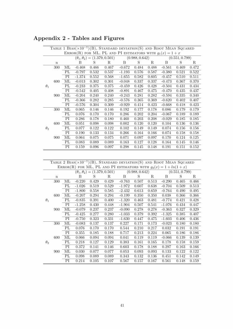
Appendix 2 - Tables and Figures

Table 1 Bias(×10−1)(B), Standard deviation(S) and Root Mean SquaredError(R) for ML, PL and PI estimators with g1(x) = 1 + x

(θ1, θ2) = (1.379, 0.501) (0.988, 0.642) (0.551, 0.799)n B S R B S R B S R

300 ML -0.468 0.466 0.467 -0.672 0.484 0.488 -0.561 0.469 0.472PL -0.797 0.532 0.537 -1.193 0.576 0.587 -0.380 0.521 0.522PI -1.374 0.552 0.568 -1.655 0.582 0.605 -0.457 0.510 0.511

600 ML -0.013 0.302 0.301 -0.048 0.337 0.337 -0.473 0.367 0.370θ1 PL -0.233 0.375 0.375 -0.459 0.426 0.428 -0.504 0.431 0.434

PI -0.542 0.405 0.408 -0.891 0.467 0.475 -0.470 0.435 0.437900 ML -0.204 0.240 0.240 -0.243 0.281 0.282 -0.594 0.335 0.340

PL -0.366 0.282 0.285 -0.576 0.365 0.369 -0.620 0.402 0.407PI -0.576 0.304 0.309 -0.929 0.414 0.423 -0.668 0.418 0.423

300 ML 0.065 0.146 0.146 0.192 0.177 0.178 0.086 0.179 0.179PL 0.076 0.170 0.170 0.286 0.202 0.204 -0.067 0.189 0.189PI 0.286 0.178 0.180 0.460 0.203 0.208 -0.029 0.185 0.185

600 ML 0.051 0.098 0.098 0.002 0.120 0.120 0.104 0.136 0.136θ2 PL 0.077 0.122 0.122 0.102 0.149 0.149 0.074 0.156 0.156

PI 0.190 0.133 0.134 0.266 0.164 0.166 0.074 0.158 0.158900 ML 0.064 0.075 0.075 0.071 0.097 0.097 0.170 0.124 0.125

PL 0.083 0.089 0.089 0.163 0.127 0.128 0.164 0.145 0.146PI 0.159 0.096 0.097 0.298 0.145 0.148 0.191 0.151 0.152

Table 2 Bias(×10−1)(B), Standard deviation(S) and Root Mean SquaredError(R) for ML, PL and PI estimators with g2(x) = 1 + ln(1 + x)

(θ1, θ2) = (1.379, 0.501) (0.988, 0.642) (0.551, 0.799)n B S R B S R B S R

300 ML -0.220 0.429 0.429 -0.763 0.507 0.513 -0.290 0.465 0.466PL -1.026 0.519 0.529 -1.972 0.607 0.638 -0.704 0.509 0.513PI -1.800 0.558 0.585 -2.432 0.613 0.659 -0.764 0.490 0.495

600 ML -0.207 0.294 0.294 -0.199 0.350 0.350 0.038 0.366 0.366θ1 PL -0.835 0.391 0.400 -1.320 0.463 0.481 -0.774 0.421 0.428

PI -1.258 0.430 0.448 -1.904 0.507 0.541 -1.076 0.434 0.447900 ML -0.079 0.237 0.237 -0.090 0.278 0.278 -0.363 0.327 0.329

PL -0.425 0.277 0.280 -1.033 0.379 0.392 -1.325 0.385 0.407PI -0.750 0.323 0.331 -1.630 0.447 0.475 -1.603 0.406 0.436

300 ML -0.083 0.137 0.137 0.227 0.171 0.173 -0.023 0.180 0.180PL 0.076 0.170 0.170 0.544 0.210 0.217 0.032 0.191 0.191PI 0.355 0.185 0.188 0.717 0.213 0.224 0.065 0.186 0.186

600 ML 0.066 0.094 0.094 0.041 0.119 0.119 -0.066 0.139 0.139θ2 PL 0.218 0.127 0.129 0.383 0.161 0.165 0.178 0.158 0.159

PI 0.372 0.141 0.146 0.603 0.178 0.188 0.297 0.163 0.166900 ML 0.030 0.077 0.077 0.053 0.093 0.093 0.133 0.122 0.122

PL 0.098 0.089 0.089 0.343 0.132 0.136 0.451 0.142 0.149PI 0.214 0.105 0.107 0.567 0.157 0.167 0.561 0.148 0.159

41

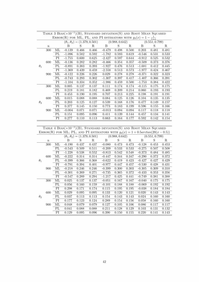
Table 3 Bias(×10−1)(B), Standard deviation(S) and Root Mean SquaredError(R) for ML, PL, and PI estimators with g3(x) = 1− 1

1+x

(θ1, θ2) = (1.379, 0.501) (0.988, 0.642) (0.551, 0.799)n B S R B S R B S R

300 ML -0.139 0.466 0.466 -0.479 0.498 0.500 0.203 0.481 0.481PL -1.096 0.582 0.592 -1.782 0.593 0.619 -0.546 0.531 0.533PI -1.755 0.600 0.625 -2.427 0.597 0.644 -0.912 0.525 0.532

600 ML -0.136 0.282 0.282 -0.466 0.354 0.357 -0.509 0.373 0.376θ1 PL -0.891 0.383 0.393 -1.927 0.476 0.513 -1.681 0.412 0.445

PI -1.369 0.439 0.459 -2.558 0.513 0.573 -1.977 0.424 0.467900 ML -0.122 0.226 0.226 0.029 0.278 0.278 -0.371 0.322 0.323

PL -0.743 0.293 0.302 -1.307 0.397 0.417 -1.407 0.366 0.391PI -1.104 0.334 0.352 -1.986 0.459 0.500 -1.753 0.384 0.422

300 ML 0.005 0.137 0.137 0.111 0.174 0.174 -0.115 0.175 0.175PL 0.219 0.181 0.182 0.469 0.209 0.214 0.060 0.193 0.193PI 0.453 0.190 0.195 0.707 0.213 0.225 0.198 0.191 0.191

600 ML 0.015 0.088 0.088 0.084 0.125 0.126 0.104 0.135 0.135θ2 PL 0.203 0.125 0.127 0.539 0.168 0.176 0.477 0.149 0.157

PI 0.377 0.145 0.150 0.773 0.183 0.199 0.596 0.155 0.166900 ML -0.004 0.071 0.071 -0.013 0.094 0.094 0.117 0.118 0.118

PL 0.151 0.095 0.096 0.411 0.139 0.144 0.457 0.134 0.141PI 0.277 0.110 0.113 0.663 0.164 0.177 0.592 0.142 0.154

Table 4 Bias(×10−1)(B), Standard deviation(S) and Root Mean SquaredError(R) for ML, PL, and PI estimators with g4(x) = 1 + 0.5arctan(20(x− 0.5))

(θ1, θ2) = (1.379, 0.501) (0.988, 0.642) (0.551, 0.799)n B S R B S R B S R

300 ML -0.190 0.437 0.437 -0.080 0.473 0.473 -0.128 0.453 0.453PL -0.543 0.509 0.511 -0.209 0.533 0.533 -0.275 0.507 0.508PI -1.228 0.538 0.552 -0.813 0.542 0.548 -0.373 0.484 0.485

600 ML -0.222 0.314 0.314 -0.447 0.344 0.347 -0.290 0.372 0.372θ1 PL -0.399 0.366 0.368 -0.622 0.419 0.423 -0.427 0.427 0.429

PI -0.791 0.394 0.401 -0.977 0.447 0.457 -0.530 0.428 0.431900 ML -0.218 0.246 0.246 -0.399 0.300 0.303 -0.305 0.309 0.310

PL -0.301 0.269 0.271 -0.735 0.365 0.372 -0.433 0.353 0.356PI -0.547 0.289 0.294 -1.217 0.425 0.441 -0.749 0.381 0.388

300 ML 0.025 0.137 0.137 -0.051 0.167 0.167 -0.040 0.175 0.175PL 0.056 0.160 0.159 -0.101 0.188 0.188 -0.069 0.192 0.192PI 0.298 0.171 0.174 0.115 0.195 0.195 -0.038 0.184 0.184

600 ML 0.029 0.095 0.095 0.133 0.120 0.121 0.020 0.143 0.143θ2 PL 0.037 0.113 0.113 0.154 0.143 0.143 0.024 0.160 0.160

PI 0.177 0.123 0.124 0.289 0.154 0.156 0.058 0.160 0.160900 ML 0.048 0.079 0.079 0.127 0.105 0.106 0.086 0.117 0.117

PL 0.041 0.088 0.088 0.211 0.128 0.129 0.103 0.131 0.132PI 0.129 0.095 0.096 0.390 0.150 0.155 0.220 0.141 0.143

42

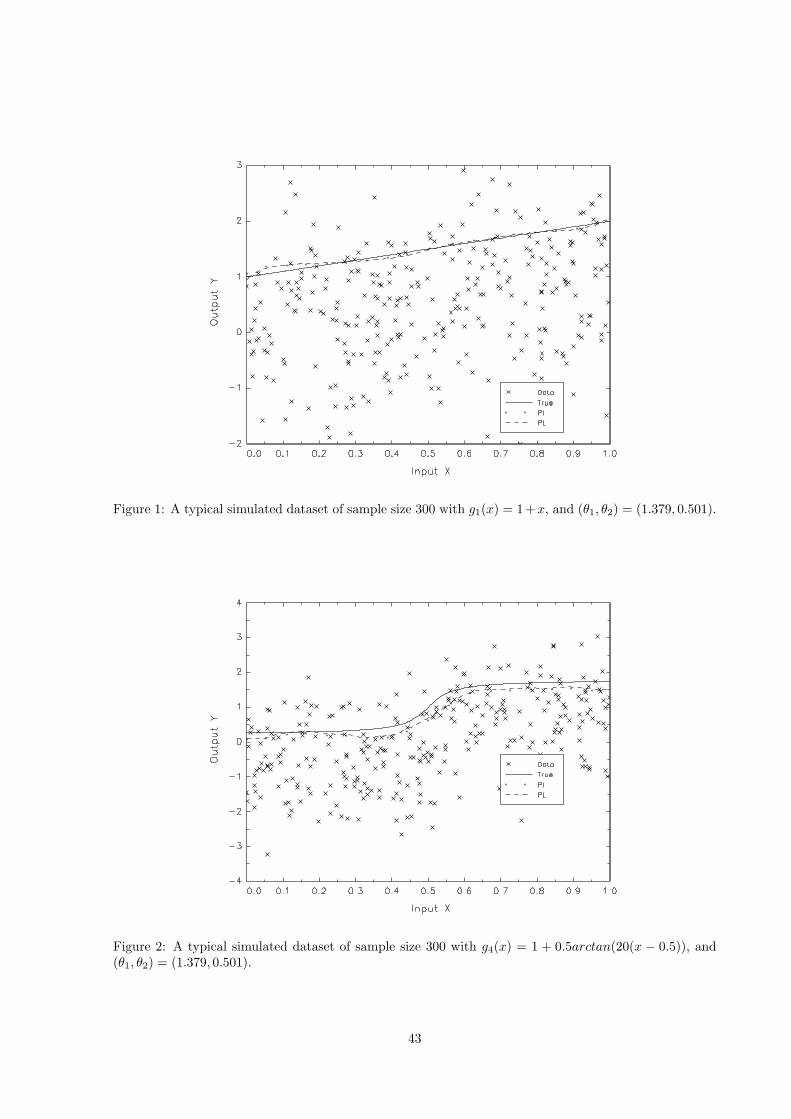
Figure 1: A typical simulated dataset of sample size 300 with g1(x) = 1 +x, and (θ1, θ2) = (1.379, 0.501).

Figure 2: A typical simulated dataset of sample size 300 with g4(x) = 1 + 0.5arctan(20(x − 0.5)), and(θ1, θ2) = (1.379, 0.501).

43

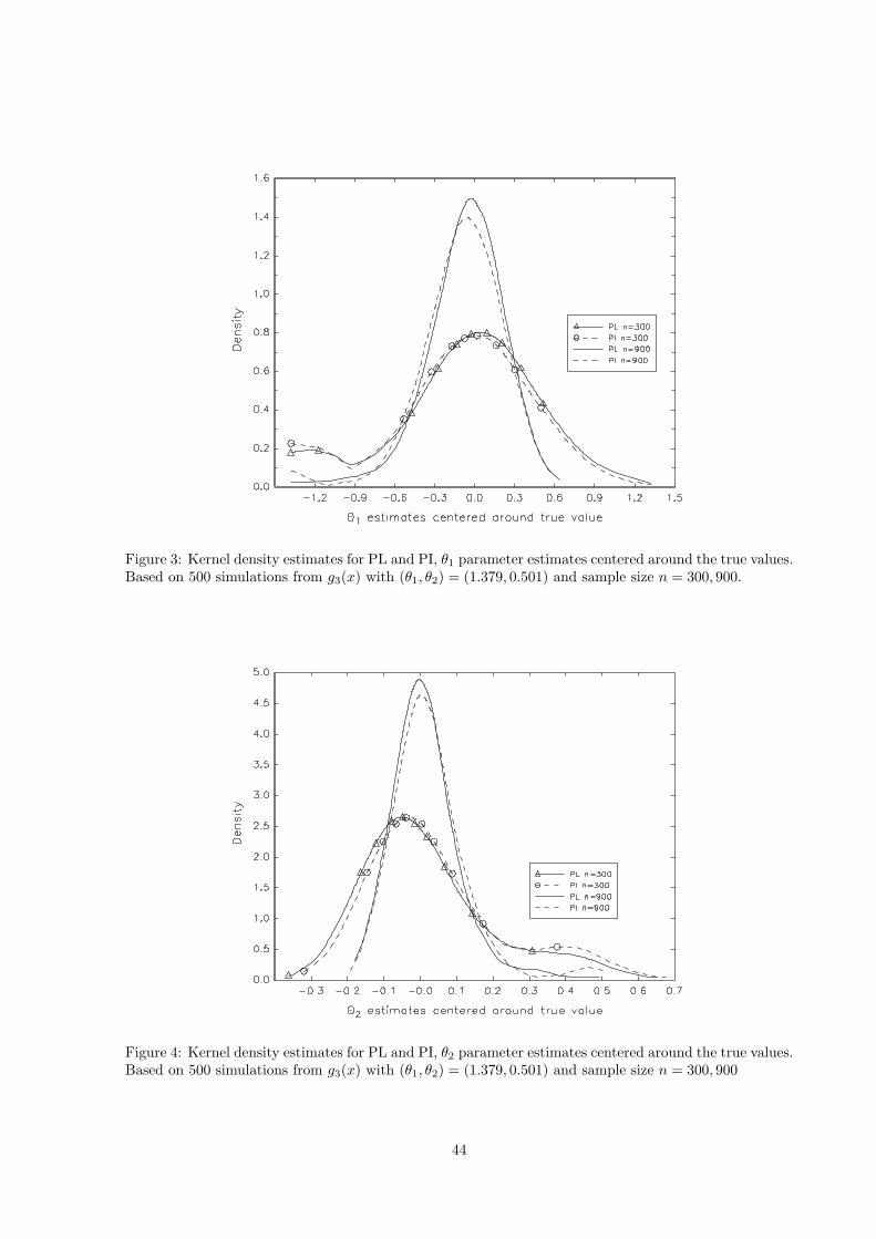
Figure 3: Kernel density estimates for PL and PI, θ1 parameter estimates centered around the true values.Based on 500 simulations from g3(x) with (θ1, θ2) = (1.379, 0.501) and sample size n = 300, 900.

Figure 4: Kernel density estimates for PL and PI, θ2 parameter estimates centered around the true values.Based on 500 simulations from g3(x) with (θ1, θ2) = (1.379, 0.501) and sample size n = 300, 900

44

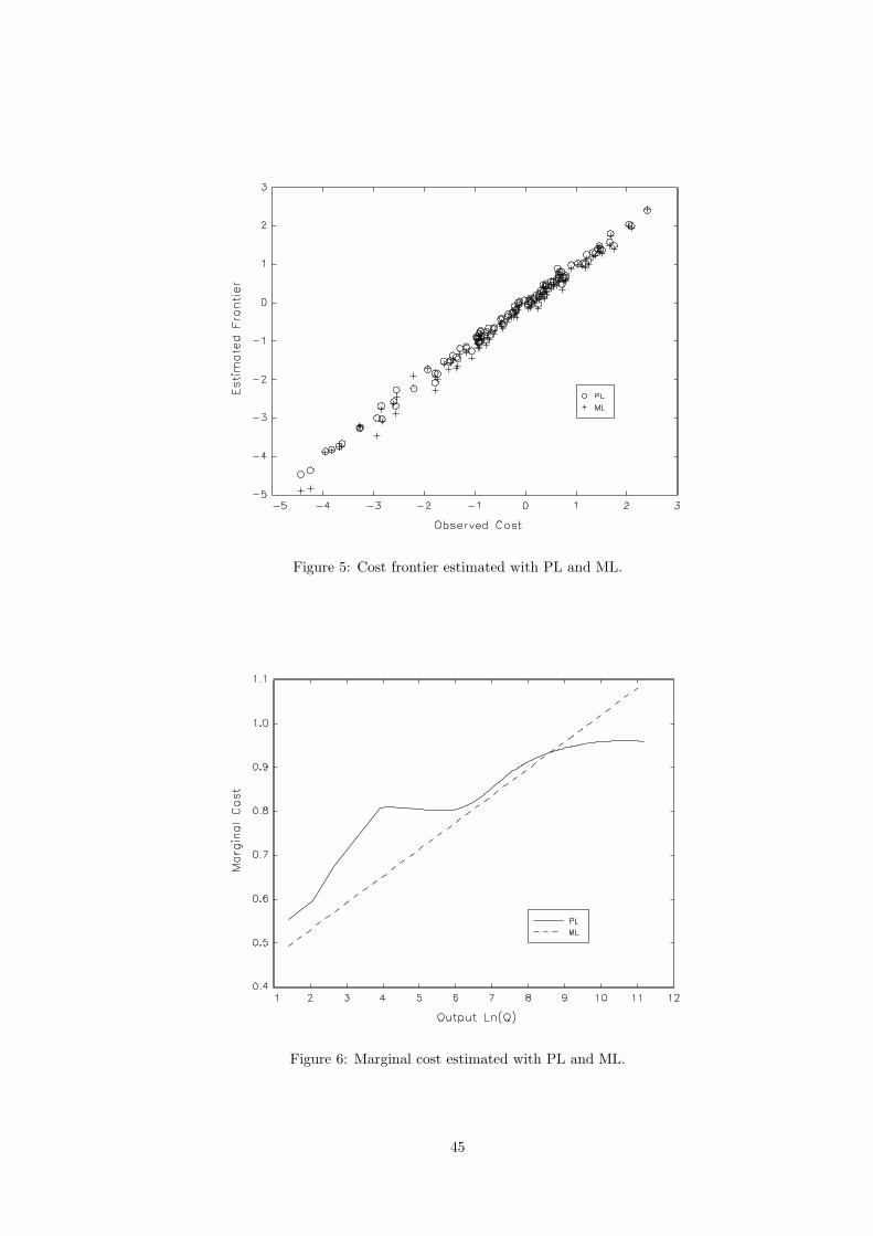
Figure 5: Cost frontier estimated with PL and ML.

Figure 6: Marginal cost estimated with PL and ML.

45

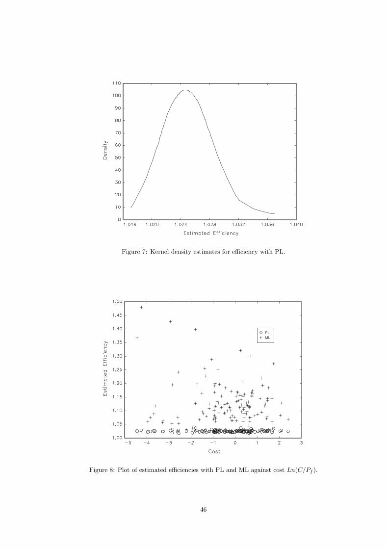
Figure 7: Kernel density estimates for efficiency with PL.

Figure 8: Plot of estimated efficiencies with PL and ML against cost Ln(C/Pf ).

46

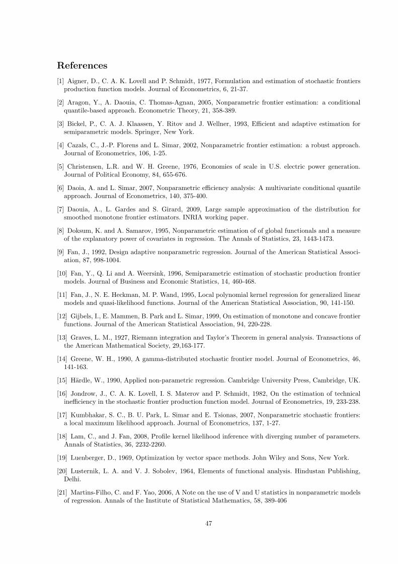
References

[1] Aigner, D., C. A. K. Lovell and P. Schmidt, 1977, Formulation and estimation of stochastic frontiersproduction function models. Journal of Econometrics, 6, 21-37.

[2] Aragon, Y., A. Daouia, C. Thomas-Agnan, 2005, Nonparametric frontier estimation: a conditionalquantile-based approach. Econometric Theory, 21, 358-389.

[3] Bickel, P., C. A. J. Klaassen, Y. Ritov and J. Wellner, 1993, Efficient and adaptive estimation forsemiparametric models. Springer, New York.

[4] Cazals, C., J.-P. Florens and L. Simar, 2002, Nonparametric frontier estimation: a robust approach.Journal of Econometrics, 106, 1-25.

[5] Christensen, L.R. and W. H. Greene, 1976, Economies of scale in U.S. electric power generation.Journal of Political Economy, 84, 655-676.

[6] Daoia, A. and L. Simar, 2007, Nonparametric efficiency analysis: A multivariate conditional quantileapproach. Journal of Econometrics, 140, 375-400.

[7] Daouia, A., L. Gardes and S. Girard, 2009, Large sample approximation of the distribution forsmoothed monotone frontier estimators. INRIA working paper.

[8] Doksum, K. and A. Samarov, 1995, Nonparametric estimation of of global functionals and a measureof the explanatory power of covariates in regression. The Annals of Statistics, 23, 1443-1473.

[9] Fan, J., 1992, Design adaptive nonparametric regression. Journal of the American Statistical Associ-ation, 87, 998-1004.

[10] Fan, Y., Q. Li and A. Weersink, 1996, Semiparametric estimation of stochastic production frontiermodels. Journal of Business and Economic Statistics, 14, 460-468.

[11] Fan, J., N. E. Heckman, M. P. Wand, 1995, Local polynomial kernel regression for generalized linearmodels and quasi-likelihood functions. Journal of the American Statistical Association, 90, 141-150.

[12] Gijbels, I., E. Mammen, B. Park and L. Simar, 1999, On estimation of monotone and concave frontierfunctions. Journal of the American Statistical Association, 94, 220-228.

[13] Graves, L. M., 1927, Riemann integration and Taylor’s Theorem in general analysis. Transactions ofthe American Mathematical Society, 29,163-177.

[14] Greene, W. H., 1990, A gamma-distributed stochastic frontier model. Journal of Econometrics, 46,141-163.

[15] Hardle, W., 1990, Applied non-parametric regression. Cambridge University Press, Cambridge, UK.

[16] Jondrow, J., C. A. K. Lovell, I. S. Materov and P. Schmidt, 1982, On the estimation of technicalinefficiency in the stochastic frontier production function model. Journal of Econometrics, 19, 233-238.

[17] Kumbhakar, S. C., B. U. Park, L. Simar and E. Tsionas, 2007, Nonparametric stochastic frontiers:a local maximum likelihood approach. Journal of Econometrics, 137, 1-27.

[18] Lam, C., and J. Fan, 2008, Profile kernel likelihood inference with diverging number of parameters.Annals of Statistics, 36, 2232-2260.

[19] Luenberger, D., 1969, Optimization by vector space methods. John Wiley and Sons, New York.

[20] Lusternik, L. A. and V. J. Sobolev, 1964, Elements of functional analysis. Hindustan Publishing,Delhi.

[21] Martins-Filho, C. and F. Yao, 2006, A Note on the use of V and U statistics in nonparametric modelsof regression. Annals of the Institute of Statistical Mathematics, 58, 389-406

47

[22] Martins-Filho, C. and F. Yao, 2007, Nonparametric frontier estimation via local linear regression.Journal of Econometrics, 141, 283-319.

[23] Martins-Filho, C. and F. Yao, 2008, A smoothed conditional quantile frontier estimator. Journal ofEconometrics, 143, 317-333.

[24] Martins-Filho, C. and F. Yao, 2010, A note on some properties of a skew-normal density. Availableat http://spot.colorado.edu/∼martinsc/Research.html

[25] Meeusen, W. and J. van den Broeck, 1977, Efficiency estimation from Cobb-Douglas productionfunctions with composed error. International Economic Review, 18, 435-444.

[26] Newey, W. and D. McFadden, 1994, Large sample estimation and hypothesis testing. In: R. F. Engleand D. L. McFadden, (Eds.), Handbook of Econometrics, Volume 4. Elsevier Science B.V., Amsterdam.

[27] Ruppert, D., S. Sheather and M. P. Wand, 1995, An effective bandwidth selector for local leastsquares regression. Journal of the American Statistical Association, 90, 1257-1270.

[28] Severini, T., 2000, Likelihood methods in statistics. Oxford University Press, Oxford.

[29] Severini, T. and W. H. Wong, 1992, Profile likelihood and conditionally parametric models. Annalsof Statistics, 20, 1768-1802.

[30] Simar, L. and P. Wilson, 2006, Statistical inference in nonparametric frontier models: recent devel-opments and perspectives. In: H. Fried, C. A. K. Lovell, and S. S. Schmidt, (Eds.), The Measurementof Productive Efficiency, 2nd edition. Oxford University Press, Oxford.

[31] Staniswalis, J., 1989, On the kernel estimate of a regression functionin likelihood based models.Journal of the American Statistical Association, 84, 276-283.

[32] Stein, J., 1954, Efficient nonparametric testing and estimation. In: Neyman, J. (Ed.), Proceedingsof the third Berkeley symposium on mathematical statistics and probability. University of CaliforniaPress, Berkeley.

[33] van der Vaart, A., 1999, Semiparametric statistics. Lecture notes, Vrije Universiteit Amsterdam.

48