Embed Size (px)
Citation preview
44 The Open Automation and Control System Journal, 2008, 1, 44-49
1874-4443/08 2008 Bentham Open
Open Access
Stochastic Optimal Control of Structural Systems
Z.G. Ying*
Department of Mechanics, Zhejiang University, Hangzhou 310027, P. R. China
Abstract: The stochastic optimal control is an important research subject in structural engineering. Recently, a stochastic optimal nonlinear control method has been proposed based on the stochastic dynamical programming principle and sto-chastic averaging method. The active and semi-active stochastic optimal control methods have been further developed for structural systems. The control saturation or bound, partial state observation, etc. have been taken into account by the sto-chastic optimal control. The present paper surveys these research developments.
INTRODUCTION
The strong nonlinear stochastic vibration of engineering structures such as tall buildings and large bridges is fre-quently caused by severe loadings such as earthquake and storm. The stochastic optimal control is an important re-search subject in structural engineering [1]. The mathematics theory of stochastic optimal control has been developed [2-4]. However, the linear-quadratic-Gauss (LQG) control method has mostly used for structural vibration control [5]. Recently, some stochastic optimal nonlinear control methods [6, 7] have been proposed, in particular, the method based on the stochastic dynamical programming principle and stochas-tic averaging method [8-17]. This control method can achieve better control effectiveness and efficiency than the LQG control method. These research developments are sur-veyed as follows: (1) stochastic optimal control law; (2) op-timal active control; (3) optimal semi-active control; (4) de-velopments of stochastic optimal control method.
STOCHASTIC OPTIMAL CONTROL LAW [8, 9]
A controlled and stochastically excited nonlinear struc-tural system with multi-degree-of-freedom can be expressed as
BUWXXFX
XXXXCXM +=
!
!++ )(),(
)(),( t
Vs &&&&&
(1)
where X is the n-dimensional structural displacement vector, Vs(X) is the structural potential, W(t) is the stochastic excita-tion vector, U is the control force vector. Rewrite Eq. (1) in the following form of quasi Hamiltonian equation:
i
iP
HQ
!
!=&
(2a)
ikik
j
ij
i
i utWfP
Hc
Q
HP ++!!= )(
"
"
"
"&
(2b)
*Address correspondence to this author at the Department of Mechanics, Zhejiang University, Hangzhou 310027, P.R. China; E-mail: [email protected]
where H is the Hamiltonian function, Qi and Pi are respec-tively displacement and momentum, Wk(t) is the stochastic excitation, assumed as Gaussian white noise, ui is the con-trol.
Apply the stochastic averaging method to system (2) yields averaged Itô stochastic differential equations. In the integrable and non-resonant case , for instance, the Itô equa-tion is
)(d)(d])([ tBtP
HumdH
srs
i
r
irrHH !+>
"
"<+=
(3)
where Hr is the first integral of Hamiltonian system, mr and σrs are respectively the averaged drift and diffusion coeffi-cients, Bs(t) is the unit Wiener process, <⋅> is the average operator. The objective of stochastic optimal control is to design a control ui which minimizes the performance index of system (2) or (3). For finite time-interval response control, the performance index is
]))((d),([0
! +=
ft
frir tHtuHLEJ "
(4a)
and for infinite time-interval ergodic control, it is
!"#=
f
f
t
ir
ft
tuHLt
J0
d),(1
lim
(4b)
where L is the performance function, Ψ is the terminal cost. Eqs. (3) and (4) constitute a stochastic optimal control prob-lem. By using the stochastic averaging method, the dimen-sion of system equations can been reduced, the dynamical programming equation becomes non-degenerate and the re-sponse control is converted into the energy control.
According to the stochastic dynamical programming principle, the dynamical programming equation can been built, for system (3) and index (4b) as
!"" =##
#+
#
#>
#
#<++ }
2
1][),({min
2
sr
skrk
ri
r
iriru HH
V
H
V
P
HumuHL
i (5)

Stochastic Optimal Control of Structural Systems The Open Automation and Control System Journal, 2008, Volume 1 45
where V is the value function. Then the optimal control law can be obtained by minimizing the left side of Eq. (5). Let function L be
><+= jiijrir uuRHguHL )(),( (6)
The optimal control is
rj
r
ijiH
V
P
HRu
!
!
!
!"=
"1*
2
1
(7)
where ∂Hr/∂Pj is a linear function of velocity generally so that ui
* is a quasi-linear damping force. The value function V is obtained by solving the following equation:
0)(
4
1
2
1 12
=!+
>"
"
"
"
"
"
"
"<!
"
"+
""
" !
#
$$
r
srj
s
i
r
ij
r
r
sr
skrk
Hg
H
V
H
V
P
H
P
HR
H
Vm
HH
V
(8)
The stochastic optimal control method above has been applied to a single-degree-of-freedom system with cubic nonlinearity and two-degree-of-freedom nonlinear system under Gaussian white noise and seismic excitations. Numeri-cal results show that the control effectiveness and efficiency by using the proposed method are better than by using the LQG method in terms of root-mean-square response (Figs. 1 and 2).
Fig. (1). Control effectiveness (K-percentage reduction in root-mean-square displacements).
Fig. (2). Control efficiency (µ-ratio of control effectiveness to nor-malized root-mean-square control).
OPTIMAL ACTIVE CONTROL [10, 11]
The optimal feedback control (7) can be implemented by active control devices, for instance, active mass damper (AMD). The optimal active control method has been applied
to the vibration control of a hysteretic column system and coupled adjacent structures.
Optimal Active Control of Hysteretic Column
A controlled and parametrically/externally excited hys-teretic column system can be expressed as
utZXtkkXX +=!+!!++ )()1()]([2 21 "#$#% &&& (9a)
1!!!=
nn
ZZXZXXAZ &&&& "# (9b)
where X is the dimensionless horizontal displacement, Z is the hysteretic force satisfying BW hysteresis Eq. (9b), η(t) and ξ(t) are respectively the vertical parametric excitation and horizontal external excitation, assumed as Gaussian white noises, u is the control. Firstly, the hysteretic force Z is separated equivalently into quasi-linear damping force and nonlinear elastic restoring force to yield equivalent non-hysteretic system
utXktX
UXHX ++=
!
!+++ )()()](22[ 2
11 "#$$ &&&
(10)
where H is the total system energy. Then applying the sto-chastic averaging method yields averaged Itô stochastic dif-ferential equation
)(d)(d])([ tHtX
HuHmdH !"+>#
#<+=
& (11)
According to the stochastic dynamical programming principle, the dynamical programming equation for system (11) and index (4b) is obtained as
!" =#
#+
#
#>
#
#<++ }
2
1)(),({min
2
22
H
V
H
V
P
HumuHL
u (12)
For the function L quadratic in control, the optimal active control is
XH
V
RX
H
H
V
Ru &
& !
!"=
!
!
!
!"=
2
1
2
1*
(13)
The response statistics of the controlled system can be evaluated by substituting the optimal control into Eq. (9a) and using the stochastic averaging method. Numerical results are shown in Fig. (3).
Fig. (3). Control effectiveness (Κ-percentage reduction in root-mean-square displacements) and efficiency (µ-ratio of control ef-fectiveness to normalized root-mean-square control) of the hys-teretic column.
0 0.1 0.2 0.3 0.4 0.5 0.6 0.7 0.8 0.9 140
45
50
55
60
65
70
75
80
K (%
)
Excitation intensity
Proposed optimal control
LQG control
0 0.1 0.2 0.3 0.4 0.5 0.6 0.7 0.8 0.9 10.48
0.5
0.52
0.54
0.56
0.58
0.6
�
Excitation intensity
Proposed optimal
LQG control
0 0.1 0.2 0.3 0.4 0.5 0.6 0.7 0.8 0.9 140
45
50
55
60
65
70
75
80
85
90
�an
d �
Excitation intensity
� (%)
� (/100)
46 The Open Automation and Control System Journal, 2008, Volume 1 Z.G. Ying
Optimal Active Control of Coupled Adjacent Structures
A controlled and coupled multi-storey structures system under seismic ground motion excitation can be expressed as
UPEMXKXCXM 111111111 )( +!=++ txg&&&&&
(14a)
UPEMXKXCXM 222222222 )( +!=++ txg&&&&&
(14b)
where X1 and X2 are respectively the displacement vectors of structures 1 and 2, x••g (t) is the seismic excitation with the KT power spectral density, U is the coupling control force vec-tor. By the structural mode transforming, reducing and sto-chastic averaging, the Itô stochastic differential equation obtained is
)(d)(d])([d ttv
BHóUQ
HHmH +>
!
!<+=
&
(15)
where H is the modal energy vector of the coupled struc-tures, Q is the modal displacement vector, v
U is the modal control force vector, m and ! are respectively the drift coefficient vector and diffusion coefficient matrix. For sys-tem (15) and index (4b), the dynamical programming equa-tion is obtained as
minU{L(H,U)+ (m+ <
!H
!&QU
v>)
T !V
!H+1
2tr(""
T !2V
!H2)} = # (16)
For the function L quadratic in control, the optimal active control is
U*= !
1
2R
p
!1(P1
T"1
#H1
#&Q1
#V
#H1
+P2
T"2
#H2
#&Q2
#V
#H2
) (17)
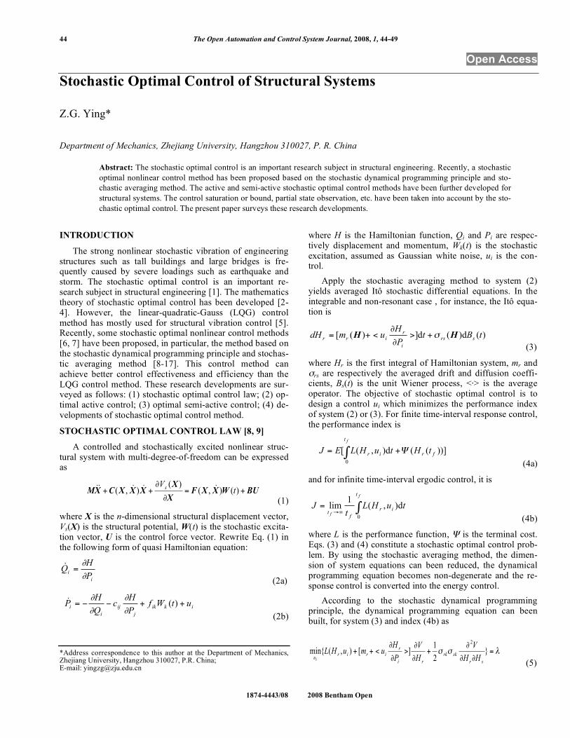
The response statistics of the controlled system can be evaluated by substituting the optimal control into Eq. (14) and using the stochastic averaging method. Numerical results are shown in Figs. 4(a) and 4(b).
OPTIMAL SEMI-ACTIVE CONTROL [12-14]
The semi-active control depends on a smaller power sup-ply and is more significant. The dynamic characteristics of semi-active control devices need to be taken into account by control. The MR damper is a classical semi-active control device, which can been described by the Bingham model or Bouc-Wen model [18, 19]. The MR-TLCD is another semi-active control device.
Semi-Active Control Law Based on the Bingham Model of MR Dampers
By applying the stochastic averaging method and sto-chastic dynamical programming principle to system (1) or (2), the optimal active control (7) can be determined. How-ever, The semi-active MR damper cannot always implement the optimal active control law. According to the Bingham model, the control produced by an MR damper is
)sgn( iiiii QFQcu && !!= (18)
The first part of control (18) is a passive control compo-nent which can be incorporated in system, and the second part of control (18) is a semi-active control component which has the amplitude Fi adjustable by the applied voltage and is in the opposite direction of velocity. If the semi-active control (18) disagrees with the optimal control, it is set to be zero. Therefore, the optimal semi-active control is
!"#
<
$%=
0,0
0),sgn(*
**
i
iiis
iF
FQFu
&
(19a)
)sgn(2
1 1*
i
rj
riji Q
H
V
P
HRF &
!
!
!
!=
"
(19b)
The efficacy of semi-active control (19) is generally lower than that of the corresponding active control (7). How-ever, under certain conditions, the relation Fi
*≥0 always holds so that the semi-active control (19) agrees with the active control (7). Thus the semi-active MR dampers can perform the optimal active control law.
Semi-Active Control Law Based on the Bouc-Wen Model of MR Dampers
The Bouc-Wen model can quite describe the dynamic characteristics of MR dampers such as hysteresis. According to this model, the control produced by an MR damper is
iiiii zQcu !""= & (20a)
1!!!=
ii n
iiii
n
iiiiii zzQzQQAz &&&& "# (20b)
Fig. (4). Control effectiveness (K) and efficiency (µ) of the cou-pled adjacent structures.
0 0.1 0.2 0.3 0.4 0.5 0.6 0.7 0.8 0.9 1123456789
1011121314151617181920
(a) 20-storey structure
0 0.1 0.2 0.3 0.4 0.5 0.6 0.7 0.8 0.9 11
2
3
4
5
6
7
8
9
10
(b) 10-storey structure
−•− displacement Κ − − displacement µ −♦− drift Κ − − drift µ
Κ and µ
Floo
r
−•− displacement Κ − − displacement µ −♦− drift Κ − − drift µ
Κ and µ
Floo
r
Stochastic Optimal Control of Structural Systems The Open Automation and Control System Journal, 2008, Volume 1 47
The coefficients ci and αi can be separated into two parts, respectively. The first parts cip and αip are constants, and the second parts are proportional to the applied voltage Ui. That is
iisipi Uccc += , iisipi U!!! += (21a,b)
Substituting semi-active control (20) and (21) into system (2), converting it into equivalent non-hysteretic system and incorporating the passive control component in the system yield
i
iP
HQ
!
!=&
(22a)
i
i
isiskik
j
ij
i
i UQ
VctWf
P
Hc
Q
HP )()(
!
!+"+
!
!"
!
!"=&
(22b)
By using the stochastic averaging method and stochastic dynamical programming, the optimal semi-active control voltage is obtained as
!"
"=
r r
iis
ii
iH
VQc
RU
2* )(2
1 &
(23)
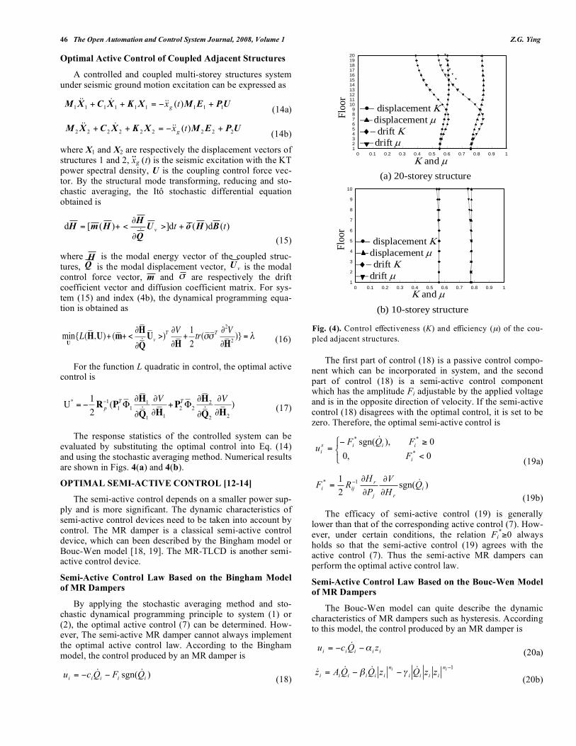
If the right-hand side of Eq. (23) is negative, voltage Ui*
is set to be zero. Under certain conditions, the right-hand side of Eq. (23) can be always non-negative. Fig. (5) shows the control effectiveness and efficiency of a single-degree-of-freedom system.
Fig. (5). Semi-active control effectiveness (Ks) and efficiency (µs) based on the Bouc-Wen model.
Semi-Active Control Law of MR-TLCD
MR-TLCD is a new semi-active control device combin-ing magneto-rheological fluid and tuned liquid column damper, which can be installed at the top floor of buildings for vibration control. A controlled building structure with an MR-TLCD under wind loading can be expressed as
Dw ft 1)( EFKXXCXM +=++ &&& (24a)
XE &&&&&T
DDD mykyuym 1)( !"=++ (24b)
Eqs. (24a) and (24b) are respectively the building and MR-TLCD equations of motion. fD is the interaction force. Fw(t) is the wind excitation with the Davenport spectrum. u is the control force produced by the MR fluid, which can be
separated into passive part up and semi-active part us. Mak-ing the modal transformation of (24a), combining it with (24b) and linearizing statistically yield
UFAZZ ++= )(t& (25)
According to the stochastic dynamical programming principle, the optimal semi-active control obtained is
!"#
<
$=
0,0
0),sgn(*
***
F
FyFus
&
(26a)
)sgn(1*yF
T&PZBR
!= (26b)
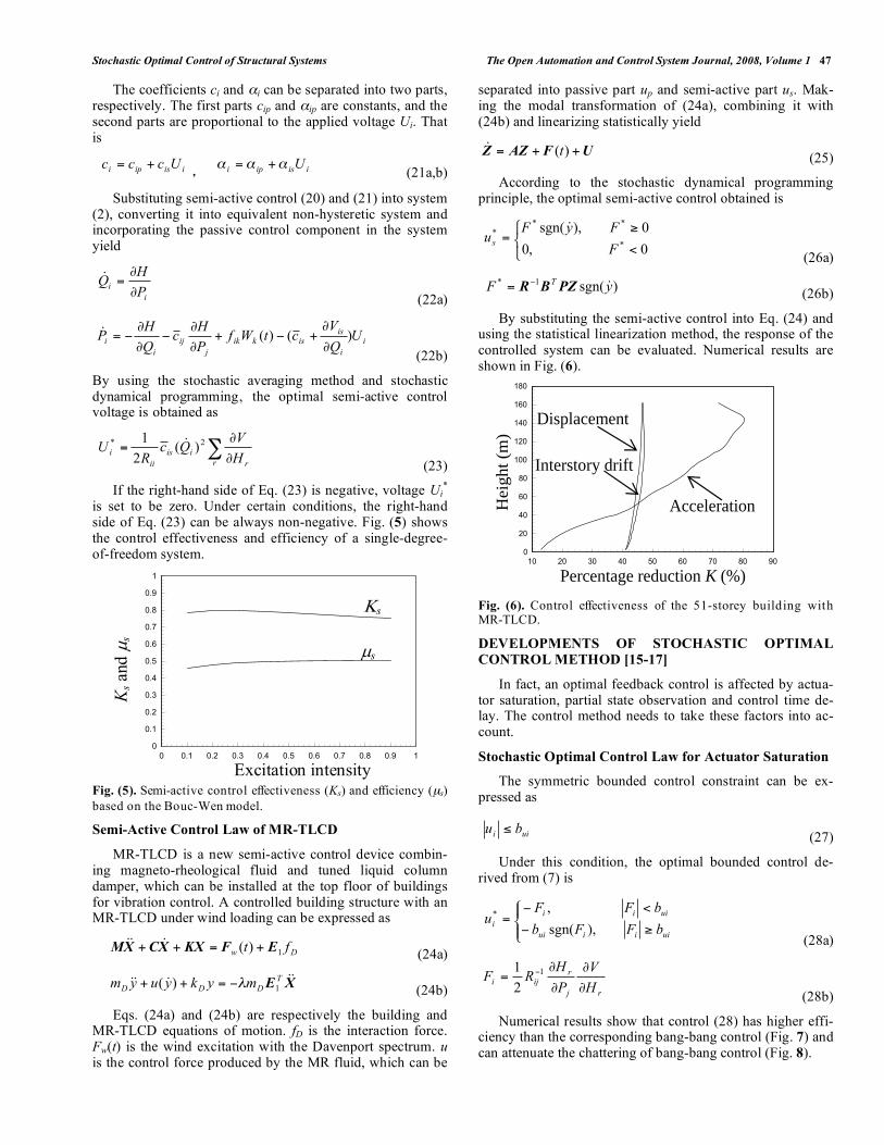
By substituting the semi-active control into Eq. (24) and using the statistical linearization method, the response of the controlled system can be evaluated. Numerical results are shown in Fig. (6).
Fig. (6). Control effectiveness of the 51-storey building with MR-TLCD.
DEVELOPMENTS OF STOCHASTIC OPTIMAL CONTROL METHOD [15-17]
In fact, an optimal feedback control is affected by actua-tor saturation, partial state observation and control time de-lay. The control method needs to take these factors into ac-count.
Stochastic Optimal Control Law for Actuator Saturation
The symmetric bounded control constraint can be ex-pressed as
uiibu ! (27)
Under this condition, the optimal bounded control de-rived from (7) is
!"
!#$
%&
<&=
uiiiui
uiii
ibFFb
bFFu
),sgn(
,*
(28a)
rj
r
ijiH
V
P
HRF
!
!
!
!=
"1
2
1
(28b)
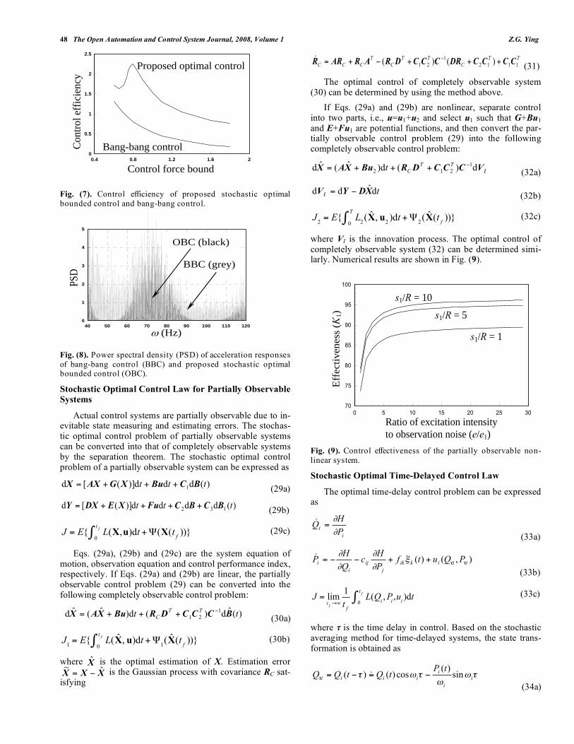
Numerical results show that control (28) has higher effi-ciency than the corresponding bang-bang control (Fig. 7) and can attenuate the chattering of bang-bang control (Fig. 8).
0 0.1 0.2 0.3 0.4 0.5 0.6 0.7 0.8 0.9 1
0
0.1
0.2
0.3
0.4
0.5
0.6
0.7
0.8
0.9
1
Ksan
d �
s
Excitation intensity
�s
�s
10 20 30 40 50 60 70 80 900
20
40
60
80
100
120
140
160
180
Hei
ght (
m)
Percentage reduction K (%)
Acceleration
Displacement
Interstory drift
48 The Open Automation and Control System Journal, 2008, Volume 1 Z.G. Ying
Fig. (7). Control efficiency of proposed stochastic optimal bounded control and bang-bang control.
Fig. (8). Power spectral density (PSD) of acceleration responses of bang-bang control (BBC) and proposed stochastic optimal bounded control (OBC).
Stochastic Optimal Control Law for Partially Observable Systems
Actual control systems are partially observable due to in-evitable state measuring and estimating errors. The stochas-tic optimal control problem of partially observable systems can be converted into that of completely observable systems by the separation theorem. The stochastic optimal control problem of a partially observable system can be expressed as
)(ddd)]([d 1 ttt BCBuXGAXX +++= (29a)
)(dddd)]([d 132 ttt BCBCFuXEDXY ++++= (29b)
J = E{ L(X,u)dt
0
tf! +"(X(t
f))} (29c)
Eqs. (29a), (29b) and (29c) are the system equation of motion, observation equation and control performance index, respectively. If Eqs. (29a) and (29b) are linear, the partially observable control problem (29) can be converted into the following completely observable control problem:
)(ˆd)(d)ˆ(ˆd 1
21 ttTT
CBCCCDRBuXAX
!+++= (30a)
J
1= E{ L(X̂, u)dt
0
tf! +"
1(X̂(t
f))} (30b)
where X̂ is the optimal estimation of X. Estimation error XXX ˆ
~!= is the Gaussian process with covariance RC sat-
isfying
TT
C
TT
C
T
CCC 1112
1
21 )()( CCCCDRCCCDRARARR +++!+=!&
(31)
The optimal control of completely observable system (30) can be determined by using the method above.
If Eqs. (29a) and (29b) are nonlinear, separate control into two parts, i.e., u=u1+u2 and select u1 such that G+Bu1 and E+Fu1 are potential functions, and then convert the par-tially observable control problem (29) into the following completely observable control problem:
!VCCCDRBuXAX d)(d)ˆ(ˆd 1
212
"+++=
TT
Ct (32a)
tdˆdd XDYV !=" (32b)
J
2= E{ L
2(X̂, u
2)dt
0
T
! +"2(X̂(t
f))} (32c)
where VI is the innovation process. The optimal control of completely observable system (32) can be determined simi-larly. Numerical results are shown in Fig. (9).
Fig. (9). Control effectiveness of the partially observable non-linear system.
Stochastic Optimal Time-Delayed Control Law
The optimal time-delay control problem can be expressed as
i
iP
HQ
!
!=&
(33a)
),()( iiikik
j
ij
i
i PQutfP
Hc
Q
HP !!"
#
#
#
#++$$=&
(33b)
J = limt
f!"
1
tf
L(Qi, P
i,u
i)dt
0
tf# (33c)
where τ is the time delay in control. Based on the stochastic averaging method for time-delayed systems, the state trans-formation is obtained as
!""
!"!! i
i
iiiii
tPtQtQQ sin
)(cos)()( #=#= &
(34a)
0.4 0.8 1.2 1.6 20
0.5
1
1.5
2
2.5
Control force bound
Con
trol
eff
icie
ncy
Bang-bang control
Proposed optimal control
40 50 60 70 80 90 100 110 1200
1
2
3
4
5
PSD
(Hz)
BBC (grey)
OBC (black)
0 5 10 15 20 25 3070
75
80
85
90
95
100
Eff
ecti
vene
ss (
K1)
Ratio of excitation intensity to observation noise (e/e1)
s1/R = 1
s1/R = 5
s1/R = 10
Stochastic Optimal Control of Structural Systems The Open Automation and Control System Journal, 2008, Volume 1 49
!"!""!! iiiiiii tPtQtPP cos)(sin)()( +=#= & (34b)
and the Itô stochastic differential equation is
dHr= [m
r(H)+ < u
i
!Hr
!Pi
>]dt +"rk(H)dB
k(t) (35a)
The corresponding performance index for infinite time-interval ergodic control is
J = limt
f!"
1
tf
L(Hr,u
i)dt
0
tf# (35b)
Eq. (35) is a non-time-delay optimal control problem and its optimal control can be determined by using the method above. The inverse transformation of (34) is
!""
!" !! i
i
iiiii
PQtQQ sincos)( +== &
(36a)
!"!"" !! iiiiiii PQtPP cossin)( +#== & (36b)
Using (36) yields the optimal time-delayed control
!)(2
1 1*
rj
r
ijiH
V
P
HRu
"
"
"
"#=
#
(37)
where (⋅)τ represents the time-delayed state function. These control methods have respectively taken into account the effects of actuator saturation, partial state observation and control time delay, and however, need to improve further.
ACKNOWLEDGEMENT
This study was supported by the Zhejiang Provincial Natural Science Foundation of China under grant no. Y607087.
REFERENCES [1] G.W. Housner, L.A. Bergman, T.K. Caughey, A.G. Chassiakos,
R.O. Claus, S.F. Masri, R.E. Skelton, T.T. Soong, B.F. Spencer and J.T.P Yao, “Structural control: past, present, and future’’, ASCE In-ternational Journal of Engineering Science, 123(9): 897-971, 1997.
[2] W.H. Fleming and R.W. Rishel, Deterministic and Stochastic Op-timal Control, Berlin: Springer-Verlag, 1975.
[3] R. F. Stengel, Stochastic Optimal Control: theory and application, New York: John Wiley & Sons, 1986.
[4] M.F. Dimentberg, D.V. Iourtchenko and A.S. Bratus, ‘‘Optimal bounded control of steady-state random vibrations’’, Probabilistic Engineering Mechanics, 15: 381-6, 2000.
[5] T.T. Soong, Active Structural Control: theory and practice, New York: John Wiley & Sons, 1990.
[6] J.N. Yang, A.K. Agrawal and S. Chen,‘‘Optimal polynomial con-trol for seismically excited non-linear and hysteretic structures’’, Earthquake Engineering and Structural Dynamics, 25: 1211-30, 1996.
[7] L.G. Crespo and J.Q. Sun, ‘‘Stochastic Optimal Control of Nonlin-ear Systems via Short-time Gaussian approximation and Cell Map-ping’’, Nonlinear Dynamics, 28: 323-42, 2002.
[8] W.Q. Zhu and Z.G. Ying, ‘‘Optimal Nonlinear Feedback Control of Quasi-Hamiltonian Systems’’, Science in China, Series A, 42: 1213-9, 1999.
[9] W.Q. Zhu, Z.G. Ying and T.T. Soong, ‘‘An Optimal Nonlinear Feedback Control Strategy for Randomly Excited Structural Sys-tems’’, Nonlinear Dynamics, 24: 31-51, 2001.
[10] W.Q. Zhu, Z.G. Ying, Y.Q. Ni and J.M. Ko, ‘‘Optimal nonlinear stochastic control of hysteretic systems’’, ASCE International Journal of Engineering Science, 126: 1027-32, 2000.
[11] Z.G. Ying, Y.Q. Ni and J.M. Ko, ‘‘Non-linear Stochastic Optimal Control for Coupled-structures System of Multi-degree-of-freedom’’, Journal of Sound and Vibration, 274: 843-61, 2004.
[12] Z.G. Ying, W.Q. Zhu and T.T. Soong, ‘‘A Stochastic Optimal semi-active Control Strategy for ER/MR Dampers’’, Journal of Sound and Vibration, 259: 45-62, 2003.
[13] Z.G. Ying, Y.Q. Ni and J.M. Ko, ‘‘A New Stochastic Optimal Control Strategy for Hysteretic MR Dampers’’, Acta Mechanical Solida Sinica, 17: 223-9, 2004.
[14] Z.G. Ying, Y.Q. Ni and J.M. Ko, ‘‘Semi-active Optimal Control of Linearized Systems with Multi-degree of Freedom and Applica-tion’’, Journal of Sound and Vibration, 279: 373-88, 2005.
[15] Z.G. Ying and W.Q. Zhu,‘‘A Stochastically Averaged Optimal Control Strategy for Quasi Hamiltonian Systems with Actuator Saturation’’, Automatica, 42: 1577-82, 2006.
[16] W.Q. Zhu and Z.G. Ying, ‘‘Nonlinear Stochastic Optimal Control of Partially Observable Linear Structures’’, Structural Engineering, 24: 333-42, 2002.
[17] Z.G. Ying and W.Q. Zhu, ‘‘A Stochastic Optimal Control Strategy for Partially Observable Nonlinear Quasi-Hamiltonian Systems’’, Journal of Sound and Vibration, 310: 184-96, 2008.
[18] S.J. Dyke, B.F. Spencer, M.K. Sain and J.D.Carlson,‘‘Modeling and Control of Magnetorheological Dampers for Seismic Response Reduction’’, Smart Materials and Structures, 5: 565-75, 1996.
[19] M.D. Symans and M.C. Constantinon, ‘‘Semi-active Control Sys-tems for Seismic Protection of Structures: a State-of-the-art Re-view’’, Structural Engineering, 21: 469-87, 1999.
Received: June 09, 2008 Revised: June 24, 2008 Accepted: June 26, 2008
© Z.G. Ying; Licensee Bentham Open.
This is an open access article licensed under the terms of the Creative Commons Attribution Non-Commercial License (http://creativecommons.org/licenses/by-nc/3.0/) which permits unrestricted, non-commercial use, distribution and reproduction in any medium, provided the work is properly cited.