Embed Size (px)
Citation preview
STOCHASTIC MODELS FOR RELIABILITY, AVAILABILITY,
AND MAINTAINABILITY
Daniel F. Silva, Ph.D.Assistant ProfessorIndustrial and Systems EngineeringAuburn University
RAM IX SummitNovember 2nd 2016
Daniel F. Silva,[email protected]
Outline
Introduction to Markov models
Examples of Markov chains in RAM
Extensions and more complex models
Computational tools for Markov models
International standards for Markov models in RAM
Summary & Conclusion

INTRODUCTION TO MARKOV MODELS
Daniel F. Silva,[email protected]
What Is a Stochastic Process?
A mathematical representation of a system that evolves over time, subject to random variation.
The state of the system at a given time is captured by a random variable 𝑋𝑛 or 𝑋 𝑡
Stochastic processes can evolve in:
◦ Discrete-time {𝑋𝑛, 𝑛 = 0,1,2… }
◦ Continuous-time {𝑋(𝑡), 𝑡 ≥ 0}
Daniel F. Silva,[email protected]
Examples of Stochastic Processes
Stock price at closing of trading day
Stock price at any given time
Inventory of multiple items at the end of each day
Traffic in a website at any given time
Failure state of a component at any given time
Failure state of several component at any given time
Daniel F. Silva,[email protected]
Applications of Stochastic Processes
Revenue management
Inventory planning
Google’s search engine
Call center staffing
Derivatives pricing
Reliability, availability and maintainability
Daniel F. Silva,[email protected]
Defining a Stochastic Process
States
◦ What are the states the system can occupy?
Events
◦ What can happen in the system that triggers a change in the state?
Probabilities
◦ What are the odds of events happening?
Daniel F. Silva,[email protected]
Markov Chains
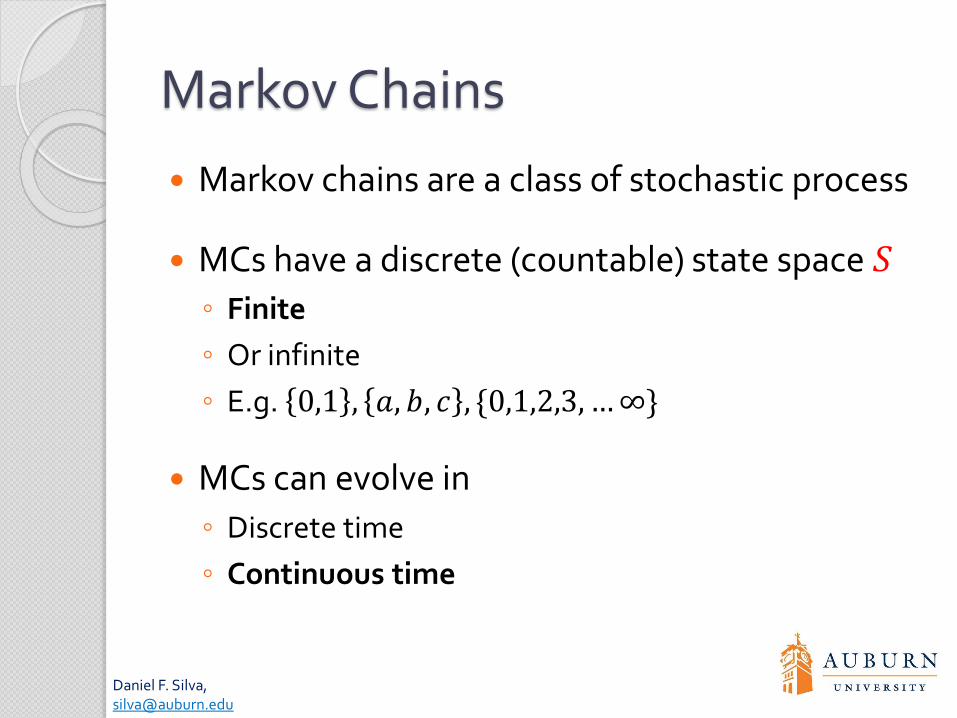
Markov chains are a class of stochastic process
MCs have a discrete (countable) state space 𝑆
◦ Finite
◦ Or infinite
◦ E.g. 0,1 , 𝑎, 𝑏, 𝑐 , {0,1,2,3, …∞}
MCs can evolve in
◦ Discrete time
◦ Continuous time
Daniel F. Silva,[email protected]
Markov Chains
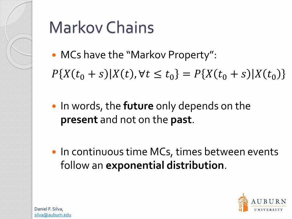
MCs have the “Markov Property”:
𝑃 𝑋 𝑡0 + 𝑠 𝑋 𝑡 , ∀𝑡 ≤ 𝑡0 = 𝑃 𝑋 𝑡0 + 𝑠 𝑋 𝑡0
In words, the future only depends on the present and not on the past.
In continuous time MCs, times between events follow an exponential distribution.
Daniel F. Silva,[email protected]
The Exponential Distribution
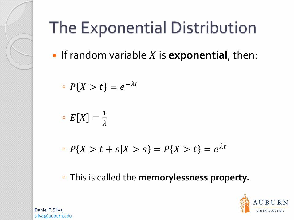
If random variable 𝑋 is exponential, then:
◦ 𝑃 𝑋 > 𝑡 = 𝑒−𝜆𝑡
◦ 𝐸 𝑋 =1
𝜆
◦ 𝑃 𝑋 > 𝑡 + 𝑠 𝑋 > 𝑠 = 𝑃 𝑋 > 𝑡 = 𝑒𝜆𝑡
◦ This is called the memorylessness property.
Daniel F. Silva,[email protected]
Markov Chains Dynamics
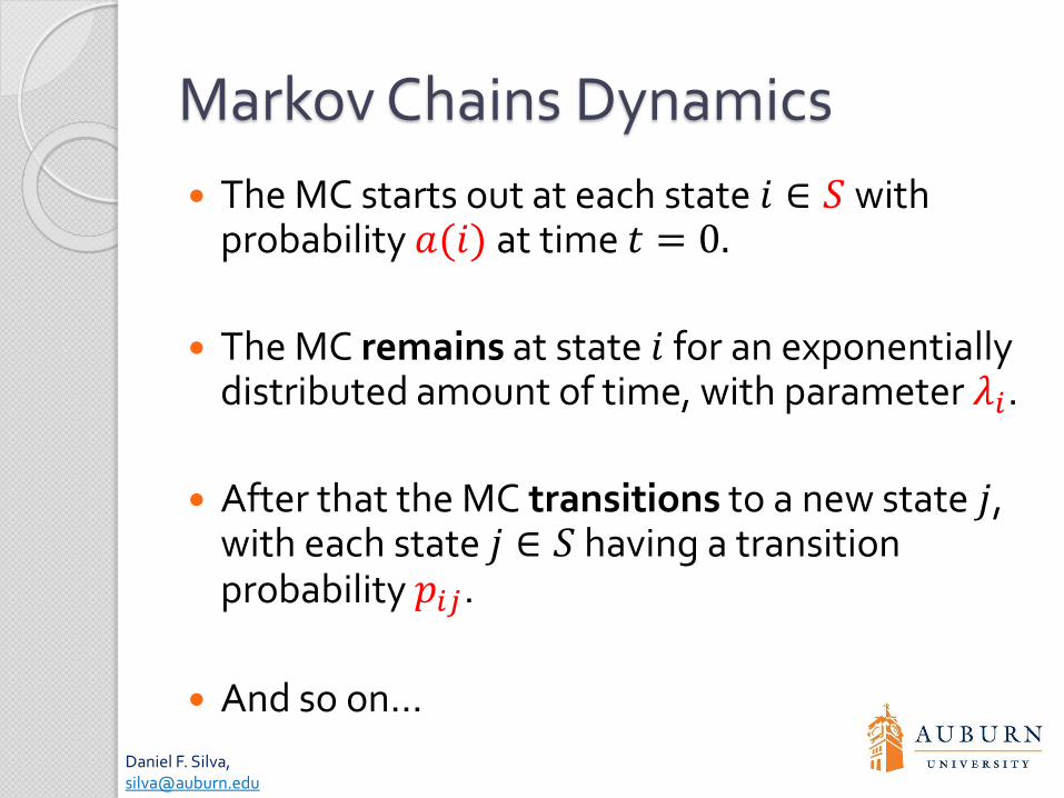
The MC starts out at each state 𝑖 ∈ 𝑆 with probability 𝑎(𝑖) at time 𝑡 = 0.
The MC remains at state 𝑖 for an exponentially distributed amount of time, with parameter 𝜆𝑖.
After that the MC transitions to a new state 𝑗, with each state 𝑗 ∈ 𝑆 having a transition probability 𝑝𝑖𝑗.
And so on…
Daniel F. Silva,[email protected]
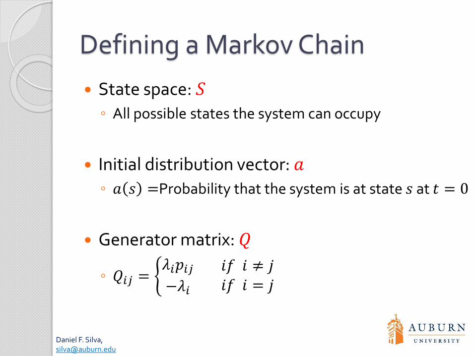
Defining a Markov Chain
State space: 𝑆
◦ All possible states the system can occupy
Initial distribution vector: 𝑎
◦ 𝑎 𝑠 =Probability that the system is at state 𝑠 at 𝑡 = 0
Generator matrix: 𝑄
◦ 𝑄𝑖𝑗 = ቊ𝜆𝑖𝑝𝑖𝑗−𝜆𝑖
𝑖𝑓 𝑖 ≠ 𝑗𝑖𝑓 𝑖 = 𝑗
Daniel F. Silva,[email protected]
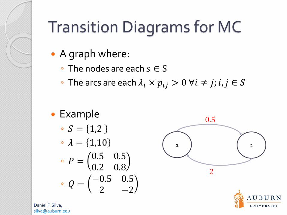
Transition Diagrams for MC
A graph where:
◦ The nodes are each 𝑠 ∈ S
◦ The arcs are each 𝜆𝑖 × 𝑝𝑖𝑗 > 0 ∀𝑖 ≠ 𝑗; 𝑖, 𝑗 ∈ 𝑆
Example
◦ 𝑆 = 1,2
◦ 𝜆 = 1,10
◦ 𝑃 =0.5 0.50.2 0.8
◦ 𝑄 =−0.5 0.52 −2
1 2
0.5
2
Daniel F. Silva,[email protected]
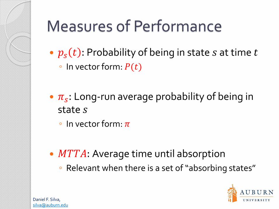
Measures of Performance
𝑝𝑠 𝑡 : Probability of being in state 𝑠 at time 𝑡
◦ In vector form: 𝑃(𝑡)
𝜋𝑠: Long-run average probability of being in state 𝑠
◦ In vector form: 𝜋
𝑀𝑇𝑇𝐴: Average time until absorption
◦ Relevant when there is a set of “absorbing states”
Daniel F. Silva,[email protected]
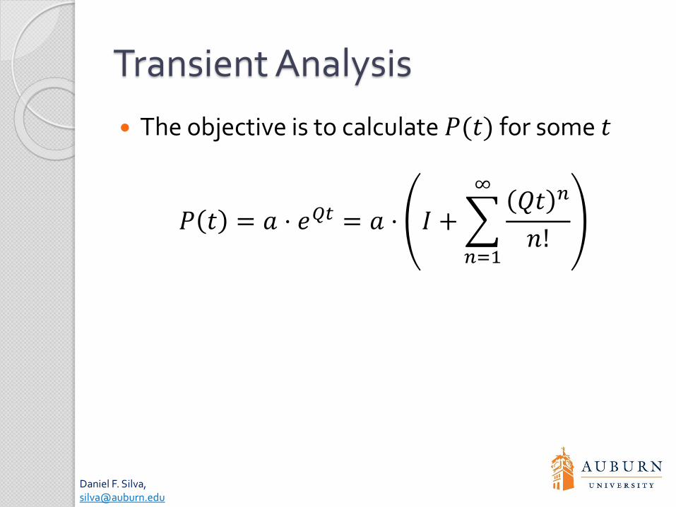
Transient Analysis
The objective is to calculate 𝑃(𝑡) for some 𝑡
𝑃 𝑡 = 𝑎 ⋅ 𝑒𝑄𝑡 = 𝑎 ⋅ 𝐼 +
𝑛=1
∞𝑄𝑡 𝑛
𝑛!
Daniel F. Silva,[email protected]
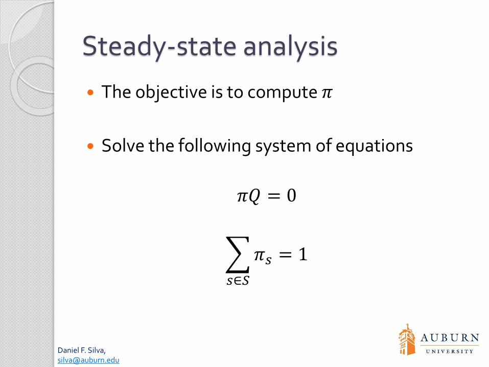
Steady-state analysis
The objective is to compute 𝜋
Solve the following system of equations
𝜋𝑄 = 0
𝑠∈𝑆
𝜋𝑠 = 1
Daniel F. Silva,[email protected]
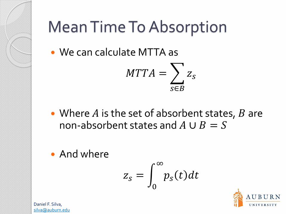
Mean Time To Absorption
We can calculate MTTA as
𝑀𝑇𝑇𝐴 =
𝑠∈𝐵
𝑧𝑠
Where 𝐴 is the set of absorbent states, 𝐵 are non-absorbent states and 𝐴 ∪ 𝐵 = 𝑆
And where
𝑧𝑠 = න0
∞
𝑝𝑠 𝑡 𝑑𝑡
EXAMPLES OF MARKOV CHAIN MODELS FOR
RELIABILITY, AVAILABILITY AND MAINTAINABILITY
Daniel F. Silva,[email protected]
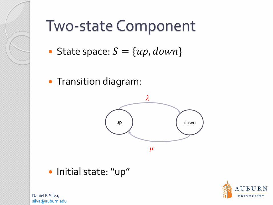
Two-state Component
Consider a single component that fails at a constant hazard rate 𝜆. Assume that repairs occur at a rate 𝜇.
◦ What is the probability that the component will be working in 1000 hours?
◦ What is the long-run availability of the component?
◦ What is the expected time to the first failure?
Daniel F. Silva,[email protected]
Two-state Component
State space: 𝑆 = {𝑢𝑝, 𝑑𝑜𝑤𝑛}
Transition diagram:
Initial state: “up”
up down
𝜆
𝜇
Daniel F. Silva,[email protected]
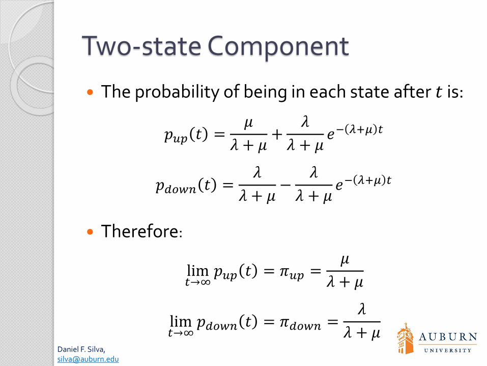
Two-state Component
The probability of being in each state after 𝑡 is:
𝑝𝑢𝑝 𝑡 =𝜇
𝜆 + 𝜇+
𝜆
𝜆 + 𝜇𝑒− 𝜆+𝜇 𝑡
𝑝𝑑𝑜𝑤𝑛 𝑡 =𝜆
𝜆 + 𝜇−
𝜆
𝜆 + 𝜇𝑒− 𝜆+𝜇 𝑡
Therefore:
lim𝑡→∞
𝑝𝑢𝑝 𝑡 = 𝜋𝑢𝑝 =𝜇
𝜆 + 𝜇
lim𝑡→∞
𝑝𝑑𝑜𝑤𝑛 𝑡 = 𝜋𝑑𝑜𝑤𝑛 =𝜆
𝜆 + 𝜇
Daniel F. Silva,[email protected]
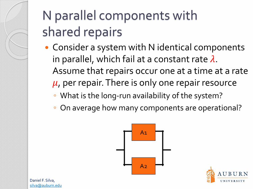
N parallel components with shared repairs Consider a system with N identical components
in parallel, which fail at a constant rate 𝜆. Assume that repairs occur one at a time at a rate 𝜇, per repair. There is only one repair resource
◦ What is the long-run availability of the system?
◦ On average how many components are operational?
A1
A2
Daniel F. Silva,[email protected]
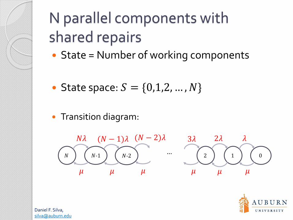
N parallel components with shared repairs State = Number of working components
State space: 𝑆 = {0,1,2, … , 𝑁}
Transition diagram:
𝑁 𝑁-1
𝑁𝜆
𝜇
1 0
𝜆
𝜇
2
2𝜆
𝜇
𝑁-2
(𝑁 − 1)𝜆
𝜇
…
3𝜆(𝑁 − 2)𝜆
𝜇𝜇
Daniel F. Silva,[email protected]
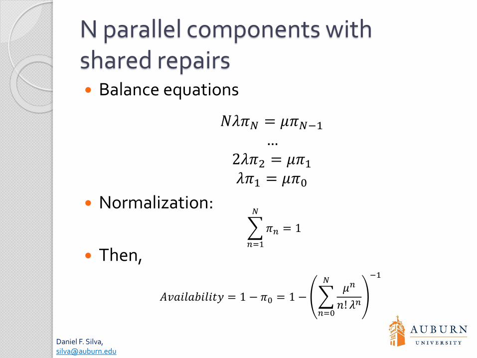
N parallel components with shared repairs Balance equations
𝑁𝜆𝜋𝑁 = 𝜇𝜋𝑁−1…
2𝜆𝜋2 = 𝜇𝜋1𝜆𝜋1 = 𝜇𝜋0
Normalization:
Then,
𝑛=1
𝑁
𝜋𝑛 = 1
𝐴𝑣𝑎𝑖𝑙𝑎𝑏𝑖𝑙𝑖𝑡𝑦 = 1 − 𝜋0 = 1 −
𝑛=0
𝑁𝜇𝑛
𝑛! 𝜆𝑛
−1
Daniel F. Silva,[email protected]
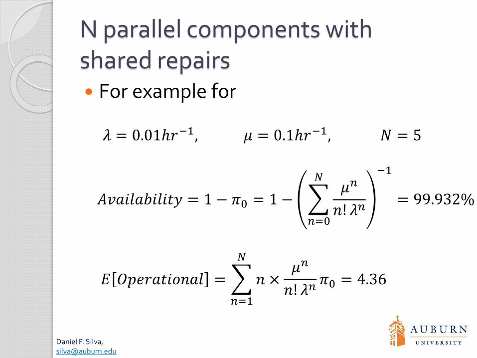
N parallel components with shared repairs For example for
𝐸 𝑂𝑝𝑒𝑟𝑎𝑡𝑖𝑜𝑛𝑎𝑙 =
𝑛=1
𝑁
𝑛 ×𝜇𝑛
𝑛! 𝜆𝑛𝜋0 = 4.36
𝐴𝑣𝑎𝑖𝑙𝑎𝑏𝑖𝑙𝑖𝑡𝑦 = 1 − 𝜋0 = 1 −
𝑛=0
𝑁𝜇𝑛
𝑛! 𝜆𝑛
−1
= 99.932%
𝜆 = 0.01ℎ𝑟−1, 𝜇 = 0.1ℎ𝑟−1, 𝑁 = 5
Daniel F. Silva,[email protected]
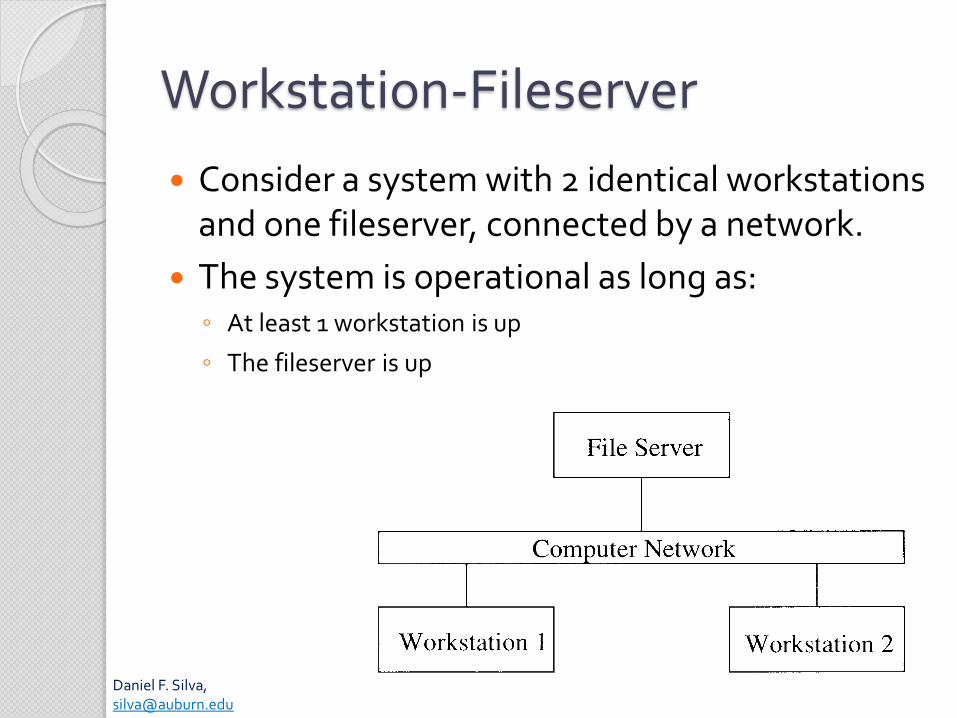
Workstation-Fileserver
Consider a system with 2 identical workstations and one fileserver, connected by a network.
The system is operational as long as:◦ At least 1 workstation is up
◦ The fileserver is up
Daniel F. Silva,[email protected]
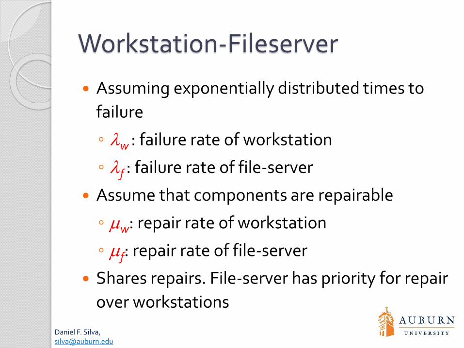
Workstation-Fileserver
Assuming exponentially distributed times to
failure
◦ w : failure rate of workstation
◦ f : failure rate of file-server
Assume that components are repairable
◦ w: repair rate of workstation
◦ f: repair rate of file-server
Shares repairs. File-server has priority for repair
over workstations
Daniel F. Silva,[email protected]
Workstation-Fileserver
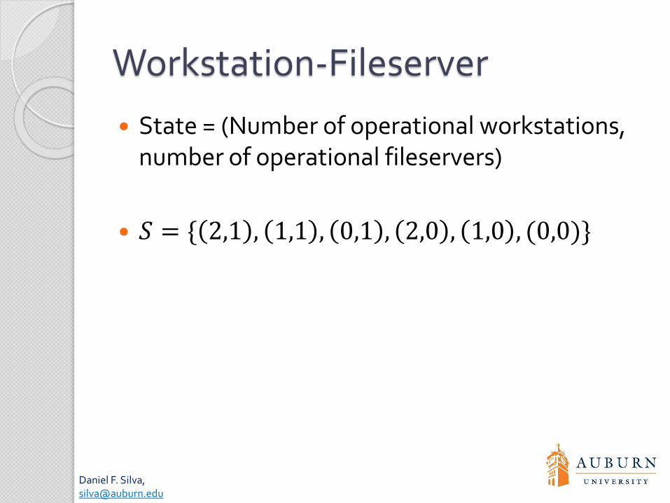
State = (Number of operational workstations, number of operational fileservers)
𝑆 = { 2,1 , 1,1 , 0,1 , 2,0 , 1,0 , (0,0)}
Daniel F. Silva,[email protected]
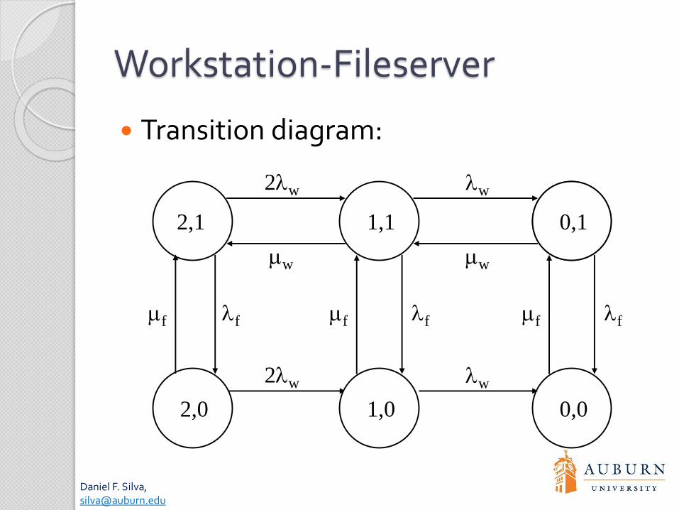
Workstation-Fileserver
Transition diagram:
0,0
2,1 1,1
1,02,0
0,1
f
2w
2w
w
w w
w
f f ff f
Daniel F. Silva,[email protected]
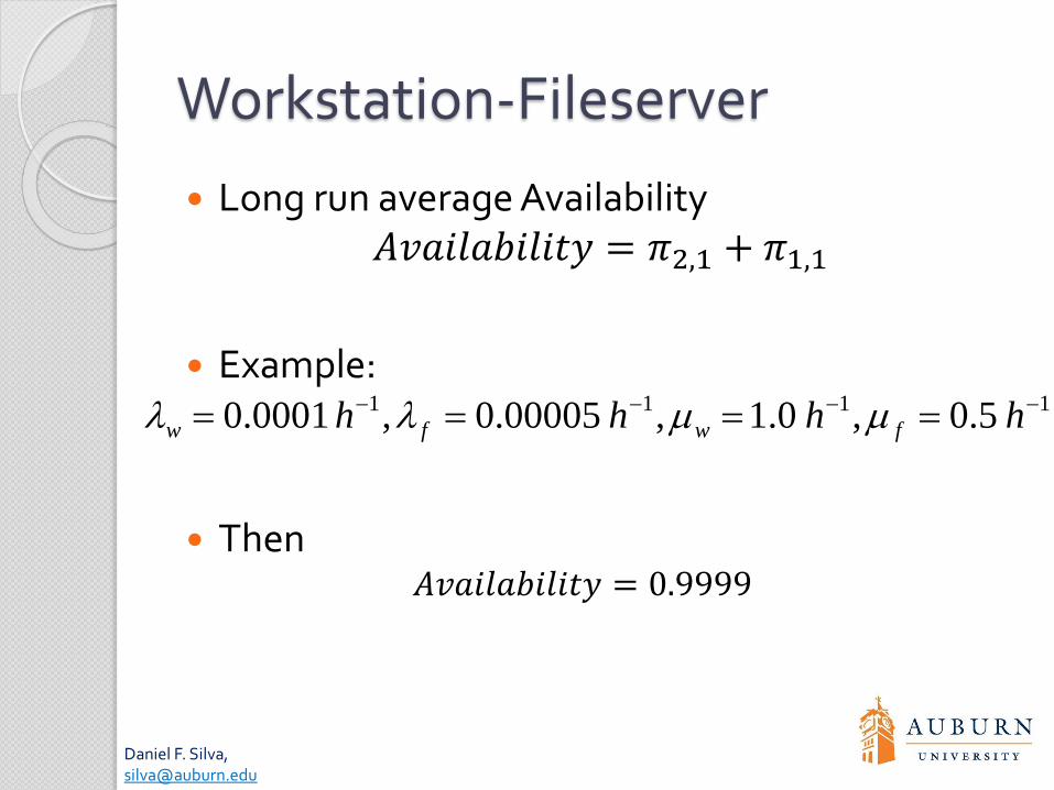
Workstation-Fileserver
Long run average Availability𝐴𝑣𝑎𝑖𝑙𝑎𝑏𝑖𝑙𝑖𝑡𝑦 = 𝜋2,1 + 𝜋1,1
Example:
Then 𝐴𝑣𝑎𝑖𝑙𝑎𝑏𝑖𝑙𝑖𝑡𝑦 = 0.9999
1111 5.0,0.1,00005.0,0001.0 hhhh fwfw
Daniel F. Silva,[email protected]
Workstation-Fileserver
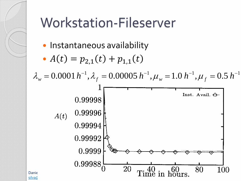
Instantaneous availability
𝐴 𝑡 = 𝑝2,1 𝑡 + 𝑝1,1 𝑡
1111 5.0,0.1,00005.0,0001.0 hhhh fwfw
Daniel F. Silva,[email protected]
Workstation-Fileserver
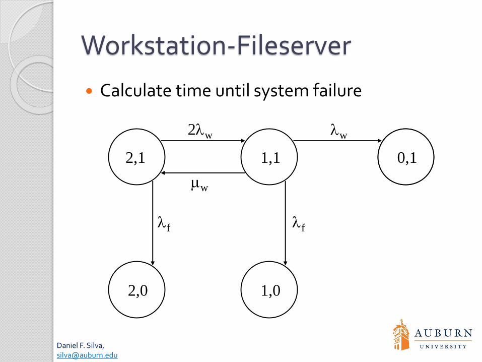
Calculate time until system failure
2,1 1,1
1,02,0
0,1
f
2w w
w
f
Daniel F. Silva,[email protected]
Workstation-Fileserver
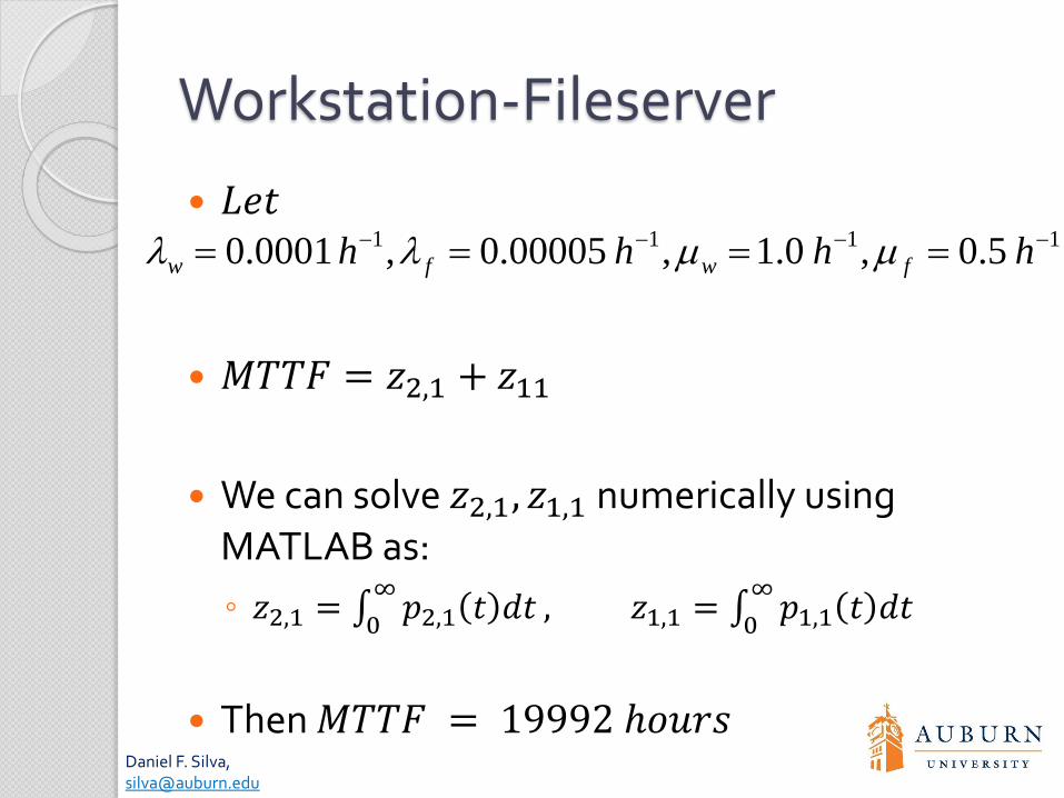
𝐿𝑒𝑡
𝑀𝑇𝑇𝐹 = 𝑧2,1 + 𝑧11
We can solve 𝑧2,1, 𝑧1,1 numerically using MATLAB as:
◦ 𝑧2,1 = 0
∞𝑝2,1 𝑡 𝑑𝑡 , 𝑧1,1 =
0
∞𝑝1,1 𝑡 𝑑𝑡
Then 𝑀𝑇𝑇𝐹 = 19992 ℎ𝑜𝑢𝑟𝑠
1111 5.0,0.1,00005.0,0001.0 hhhh fwfw
Daniel F. Silva,[email protected]
Workstation-Fileserver
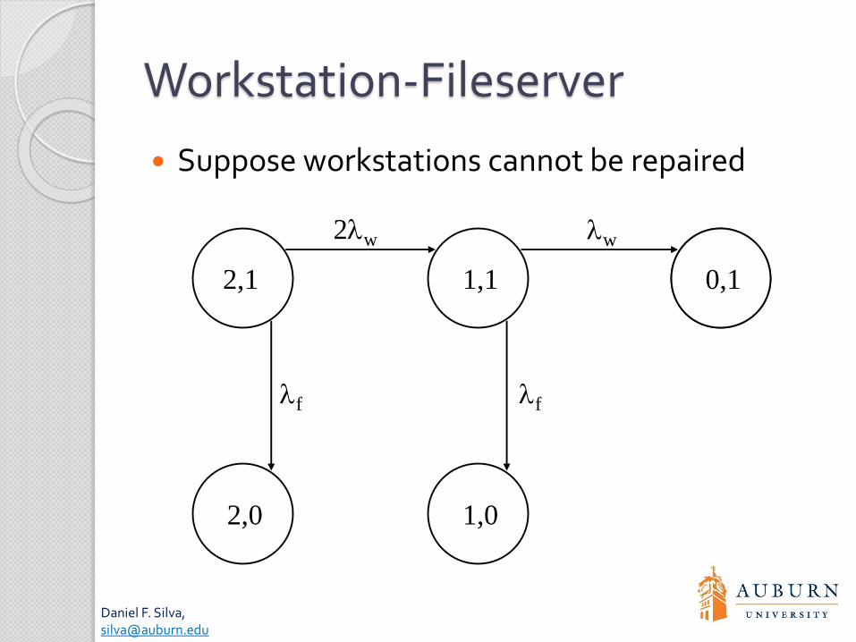
Suppose workstations cannot be repaired
2,1 1,1
1,02,0
0,1
f
2w w
f
Daniel F. Silva,[email protected]
Workstation-Fileserver
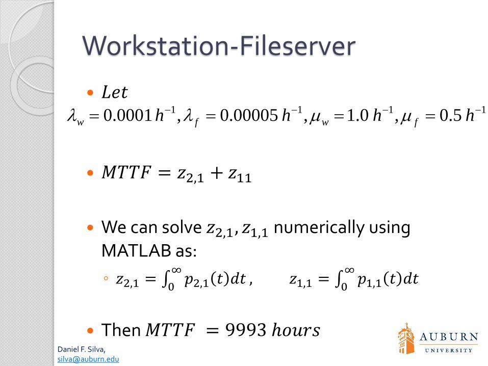
𝐿𝑒𝑡
𝑀𝑇𝑇𝐹 = 𝑧2,1 + 𝑧11
We can solve 𝑧2,1, 𝑧1,1 numerically using MATLAB as:
◦ 𝑧2,1 = 0
∞𝑝2,1 𝑡 𝑑𝑡 , 𝑧1,1 =
0
∞𝑝1,1 𝑡 𝑑𝑡
Then 𝑀𝑇𝑇𝐹 = 9993 ℎ𝑜𝑢𝑟𝑠
1111 5.0,0.1,00005.0,0001.0 hhhh fwfw
EXTENSIONS AND MORE COMPLEX MODELS
Daniel F. Silva,[email protected]
Infinite Markov Chains
Suppose that your system consists of infinitely many states.
Example: The state represents the number of components awaiting repair, from an infinite pool.
Some infinite-state MCs are well understood◦ Traditional queues M/M/1, M/M/c, etc.◦ So-called quasi-birth-death processes.
These kinds of models can be solved by◦ Analytical methods (for queues)◦ Matrix-Analytic methods (for quasi-birth-death processes). ◦ Fluid approximations to a continuous system
Daniel F. Silva,[email protected]
Phase-type Distributions
Suppose that not all times are exponential
Example: Repair times a “nearly” deterministic.
PH-type distributions allow us to model the holding times at some states as other distributions.
PH-type distributions use a new MC to model a single transition.
Some distributions that can be well approximated by PH-type are:
◦ Erlang
◦ Deterministic
◦ Hyper- and Hypo-exponential
Daniel F. Silva,[email protected]
Markov Decision Process (MDP)
Suppose you can make a decision at each transition.
Example: Choose which component gets a repaired.
MDPs add an Action Space 𝐴 to the definition of a MC.
Now the problem is not just determining performance.
We choose a policy (the action to take in each state).
The objective is to optimize a certain measure of performance. Like
◦ Maximize time to failure
◦ Maximize average availability
◦ Maximize number of repairs

COMPUTATIONAL TOOLS FOR MARKOV MODELS

Daniel F. Silva,[email protected]
Software for Markov Chains
SMCSolver
Butools
SHARPE
MKV
jMarkov
◦ Available at www.jmarkov.org
Daniel F. Silva,[email protected]
jMarkov
Object-oriented framework for Markov models
Designed for modeling and solving
Coded in Java
Can be imported into other programs
Consists of four modules:◦ Core module: General finite MCs
◦ jQBD: Highly structured infinite MCs
◦ jPhase: Structured MCs with phase-type times
◦ jMDP: Markov Decision Processes
Daniel F. Silva,[email protected]
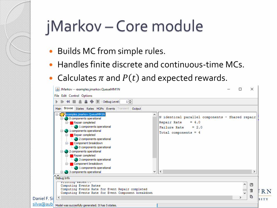
jMarkov – Core module
Builds MC from simple rules.
Handles finite discrete and continuous-time MCs.
Calculates 𝜋 and 𝑃 𝑡 and expected rewards.
Daniel F. Silva,[email protected]
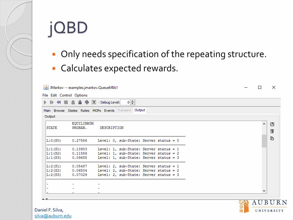
jQBD
Only needs specification of the repeating structure.
Calculates expected rewards.
Daniel F. Silva,[email protected]
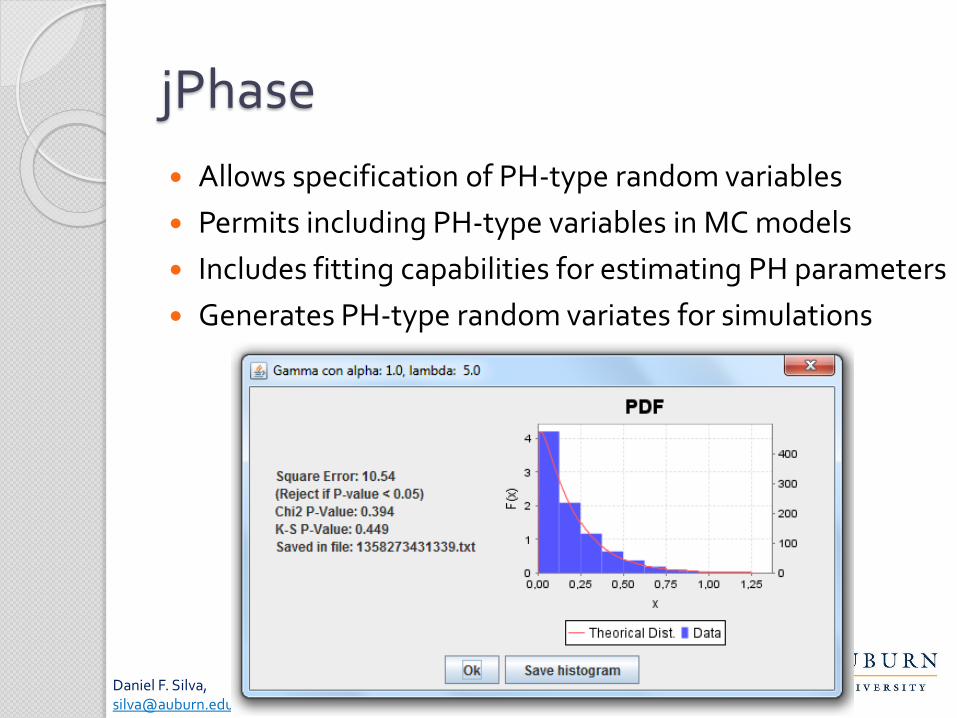
jPhase
Allows specification of PH-type random variables
Permits including PH-type variables in MC models
Includes fitting capabilities for estimating PH parameters
Generates PH-type random variates for simulations
Daniel F. Silva,[email protected]
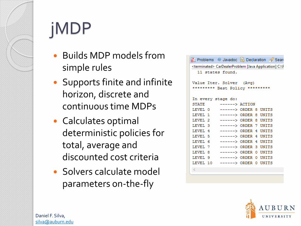
jMDP
Builds MDP models from simple rules
Supports finite and infinite horizon, discrete and continuous time MDPs
Calculates optimal deterministic policies for total, average and discounted cost criteria
Solvers calculate model parameters on-the-fly

INTERNATIONAL STANDARDS FOR APPLYING FOR MARKOV
MODELS IN RAM

Daniel F. Silva,[email protected]
IEC Standards
The International Electrotechnical Commission (IEC) has 2 standards concerning Markov modeling techniques:
◦ IEC 61165: Application of Markov techniques
◦ IEC 61508: Functional safety of electrical/ electronic/ programmable electronic safety-related systems

Daniel F. Silva,[email protected]
IEC 61165
Provides guidance on the application of Markov techniques to model and analyze a system and estimate reliability, availability, maintainability and safety measures.
◦ Gives an overview of available methods.
◦ Reviews the relative merits of each method and their applicability.

Daniel F. Silva,[email protected]
IEC 61508
Part 1: General requirements
Part 2: Requirements for electrical/ electronic/ programmable safety-related systems
Part 3: Software requirements
Part 4: Definitions and abbreviations
Part 5: Examples of methods for the determination of safety integrity levels
Part 6: Guidelines on the application of IEC 61508-2 and -3
Part 7: Overview of techniques and measures
SUMMARY &CONCLUSION
Daniel F. Silva,[email protected]
Conclusions
Markov model are a powerful mathematical modeling technique.
Markov Chains can be used in many applications of Reliability, Availability and Maintainability
Markov models can provide exact analytical solutions to small problems.
More elaborate Markov models can incorporate decision-making, non-exponential distributions and other extensions.
Computational tools, such as jMarkov, can be used to solve large scale Markov models easily.

THANK YOU
Contact:Daniel F. Silva