STOCHASTIC DEMAND FORECAST AND INVENTORY MANAGEMENT OF A SEASONAL PRODUCT IN A SUPPLY CHAIN SYSTEM

A Dissertation

Submitted to the Graduate Faculty of the Louisiana State University and

Agricultural and Mechanical College In partial fulfillment of the

Requirements for the degree of Doctor of Philosophy

in

The Interdepartmental Program In Engineering Science

by Mohammad Anwar Ashek Rahman

B.S., Bangladesh University of Engineering and Technology, 1995 M.E., Bangladesh University of Engineering and Technology, 1998

M.S., Louisiana State University, 2003 M.App.Stat., Louisiana State University, 2007

May, 2008

ii

ACKNOWLEDGEMENTS

I would like to thank my Professor Bhaba R. Sarker, chairman of my doctoral committee,

for his invaluable support, advice, and encouragement in bringing this research work to a

successful completion. He has taught me a great many things, guided me as to how to deal with

new problems.

I would also like to express my gratitude to all members of my dissertation committee,

namely Dr. Lawrence Mann Jr. of Industrial Engineering Department, Dr. Luis Escobar of

Experimental Statistics Department, Dr. Ralph Pike of Chemical Engineering Department and

Dr. Guoli Ding of Mathematics Department for the assistance rendered to me. Their

suggestions and comments helped improve the quality of this research. I like to convey my

special thanks to Dr. Mann for providing suggestions to improve the readability and for his

comments. I also feel thankful to Dr. Jack Helms, Graduate School Representative, for his

useful suggestions regarding various aspects of my research work. I would like to thank all the

people at Louisiana State University who welcomed me with enthusiasm and encouragement.

This is a major milestone in my life for which I wish to thank my parents and family as

well. Had I not received their inspiration, I might not have been able to accomplish this work. I

would also like to thank all my colleagues and friends for their sincere support during my

graduate study.

iii

TABLE OF CONTENTS

ACKNOWLEDGEMENTS…………………………….………………..………….…..……... ii

LIST OF TABLES………………………………………………………….……..……..……. vi

LIST OF FIGURES………………………………………………………………...……...…...vii ABSTRACT…………………………………………………………………………..……… viii CHAPTER 1 INTRODUCTION ……………………………...……………………....…...…....1

1.1 Study Context ..…………...…………………………..…………………......…..…1 1.2 Problem Statement……………………………………..…………………….….…3 1.3 Research Goals ……………………………………….…….…….…….…............ 4 1.4 Research Objectives……………….……………...….……..……......……..…...…4 1.5 Solution Approach …………………………………….….………………..…….. 6 1.6 Scope and Opportunities……………………………….….……….………......…..7 1.7 Actual Time Series Data...………………………………...….……...……....…….8 1.9 Organization of the Dissertation………………………..……………..…...........…8

CHAPTER 2 LITERATURE REVIEW…….……………………...…...……………….….….10

2.1 Demand Forecasts Using Bayesian Procedure ………………………......…....….10 2.2 Time Series Autoregressive Models.……………………………….………….…12 2.3 Inventory Models………………………………………………….….……......... 13 2.4 Limitations of the Past Research ………………………………………….….…. 15 2.5 Overcoming the Limitations …………………………………...…….….……….16

CHAPTER 3 BAYESIAN FORECASTING MODEL FOR SEASONAL DEMAND ….…...17

3.1 Demand Model Formulation ………………………………………..………..…..19 3.2 Bayesian Procedure in Demand Model ……………………………………..……20 3.3 Application of Demand Model ……………………………………………..……22

3.4 Sub-Models ……………………………………………………………………... 23 3.4.1 Algorithm 3.1 (Steps to Derive the Prior Values) …….….………..….…...24 3.4.2 Bayesian Probability Model (B-P Model) ……………..…………......….. 25 3.4.3 Sample Calculation (B-P Model) …...…….…………………………..….. 26 3.4.4 Bayesian Probability Model with Incomplete Data (BP-I Model) ………. 27

3.5. Forecasting Errors and Model Validity…………………………………...……...28 3.6. Summary ………………………………………………………………….…..…31

CHAPTER 4 THE ARIMA APPROACH TO FORECASTING SEASONAL DEMAND .... 32

4.1 Fundamental of the ARIMA Approach (F-ARIMA) ……………………..………33 4.1.1 Difference Operator to Eliminate Increasing Trend ……………………....34 4.1.2 Periodic Difference Operator to Eliminate Periodic Increase ……………. 35

4.2 Application of Box-Jenkins Methodology ………………………………..…….. 37 4.2.1 F-ARIMA Model Identification ……………………………...……….……37 4.2.2 Parameters Estimation of F-ARIMA Model ……………...………….…….41

iv

4.2.3 Diagnostic Checking and Model Validation .………….……………….….43 4.3 Point Forecast with F-ARIMA Model ………………………………...…….....…43 4.4 Forecast Results by F-ARIMA Model …………………………….………..…….44 4.5 Bayesian Sampling-based ARIMA Model (BS-ARIMA) …………….…..……... 46

4.5.1 Bayesian Computation at BS-ARIMA Model ……………………..…..….. 46 4.5.2 Forecast Results of BS-ARIMA Model from Incomplete Data ……..……..49

4.6 Forecast Using Adaptive Exponential Smoothing Technique ……………...……50 4.7 Forecast Performance and Model Validation…………..…………………..…… 52 4.8 Summary ……………………………………………..………………….……….53

CHAPTER 5 INVENTORY COST REDUCTION USING IMPROVED FORECASTING…55

5.1 Model Description……………………………………………………..….…....…55 5.2 Procedure to Compute Optimal Inventory Cost …..…………………….…....…. 56 5.3 Cost Components to Determine the Customer Service Level …………….….......57 5.4 Newsvendor Procurement Model………………………………………...….....…57

5.4.1 Expedite Cost Factors…………………………………….….............…… 58 5.4.2 Urgent Leadtime Cost Function…………………………….........….....…. 59 5.4.3 Cost Minimization in Newsvendor Model……………………………....... 60 5.4.4 Numerical Example: (Newsvendor Inventory Policy)……..………………61

5.5 Alternate Inventory Policy: (Periodic Review) …………………..…….…...……62 5.6 Selection of Order Points……………………………………………….…..….....63

5.6.1 Obtaining Order Points by Considering Forecast Errors ………….…..….........63 5.6.2 Numerical Illustration (Order Points)………………………………....….. 64

5.7 Optimal Inventory Cost ……………………………………………….…..…..… 65 5.7.1 Optimal Inventory Cost Using Dynamic Programming…….……………. 66 5.7.2 Determining Inventory Costs for All Forecasts …………………….....…. 67

5.8 Comparison of Forecasting Methods …………………………………….…...… 69 5.9 Summary………………………………….…………………………….….….….70

CHAPTER 6 CONCLUSION AND FUTURE RESEARCH……………………….……..….71 6.1 General Conclusion ………………………………………………..…….…...……72 6.2 Future Research Direction…………………………………….…….………...……75

6.2.1 Product Subject to Obsolescence: …………………..…….…….…………75 6.2.2 New Products: …………………………………………….………….……75 6.2.3 Products Sensitive to Economic Conditions:……………….……..….……76

REFERENCES………………………………………..……………………….………….……77

APPENDIX A: BAYESIAN PROBABILITY MODELS…………….…………………...…..80

APPENDIX B: ARIMA AND BAYESIAN ARIMA MODELS ….………………….……….86

APPENDIX C: INVENTORY COST REDUCTION MODELS ………………....…………100

VITA……………………………………………………………………….…………………106

v

LIST OF TABLES

Table 3.1: The structure of finding expected prior values ………………………..….….….….24

Table 3.2: Projected demand averaging the sample data ……………………………….……..25

Table 3.3: Prior and posterior parameters derived by B-P model for 2005 ……………….…..26

Table 3.4: Projected demand averaging the sample data ……………………………………...27

Table 3.5: Prior and posterior parameters derived by BP-I for 2005 ………………..…….…..28

Table 3.6: PE, MAD, TS for B-P and BP-I models (units in million)………………...……..…29

Table 4.1: Steps of F-ARIMA methodology for time series modeling ……………….………..37

Table 4.2: AIC and BIC values for various F-ARIMA models …………………………..….... 40

Table 4.3: Autocorrelation check of F-ARIMA residuals ………………………………….…. 41

Table 4.4: Estimated values of the F-ARIMA parameters …………………………….……….41

Table 4.5: Forecast results by F-ARIMA model (0,1,1)(1,1,0)12 (units in million) ……….….. 45

Table 4.6: Values of dummy variable for July to December, 2004 (units in million)……..…. 49

Table 4.7: Demand Forecast by BS-ARIMA model (units in million) ……………………..…. 50

Table 4.8: Forecast results by M-ES model (units in million) ..…………………….…….…... 51

Table 4.9: Forecast by F-ARIMA, BS-ARIMA and M-ES models (units in million) …….…… 52

Table 5.1: Unit costs applied to the inventory model………………………………..…..….….57

Table 5.2: Probability of stock out and corresponding safety factor………………..…..…….. 64

Table 5.3: Order point derived by (B-P) Forecasting Model ……………………...…..….….. 64

Table 5.4: Order quantity for stage-2 by Newsvendor policy (units in million)….……...…… 65

Table 5.5: Order quantity for stage-2 by Periodic Review policy (units in million)…….…… 65

Table 5.6: Inventory quantity and procurement cost by B-P model (units in million)………...66

Table 5.7: Inventory quantity and replenishment time for stage-2 (units in million)…….…... 67

vi

Table 5.8: Inventory cost using newsvendor policy for stage-2, 2005……….……………..….68

Table 5.9: Inventory quantity by newsvendor policy at stage-2, 2005 (units in million)……....68

Table 5.10: Inventory cost based on periodic review inventory policy…………….……….....69

Table 5.11: Inventory replenishment quantity by periodic review at stage-2, 2005 (units in million)………………………………………………………………………....…..69

Table 5.12: Inventory cost for each forecasting models and actual demand……………….…. 70

vii

LIST OF FIGURES

Figure 1.1: Supply-demand flow system in a supply chain ………………..……………………2 Figure 1.2: A two-stage inventory model ……………………………….….……...……………3 Figure 1.3: Activities of probability distribution models ……………………………………… 5 Figure 1.4: Activities of time series forecasting models …………………….………………….6 Figure 3.1: Variation of demand data for apparel product (Sources: U.S. Department of Commerce, Office of Textiles and Apparel) ..…………………………….………17 Figure 3.2: Flow diagram for Bayesian computation …………………….…………….….….25 Figure 3.3: Comparison of forecasts with actual demand …………….…………….….…..….29

Figure 3.4: Error comparison of all models ……..……………………………………..…..…..30 Figure 3.5: Summaries of tracking signals of the models ……………………………….….…30 Figure 4.1: Time plot of apparel demand data series after differencing ……………….…….. 38 Figure 4.2: ACF and Partial ACF of differenced demand data …………………….….….…...39 Figure 4.3: Flow chart for F-ARIMA estimation process ………………………………..…….42 Figure 4.4: Comparison of forecast and actual demand ……………………….………..……..53 Figure 4.5: Tracking signal of the F-ARIMA, BS-ARIMA and M-ES models …………..……..53

viii

ABSTRACT

Estimation of seasonal demand prior to an active demand season is essential in supply chain

management. The business cycle of the seasonal demand is divided into two stages: stage-1, the

slow-demand period, and stage-2, the peak-demand period. The focus here is to determine an

appropriate demand forecast for the peak-demand period. In the first set of forecasting model, a

standard gamma and an inverse gamma prior distribution are used to forecast demand. The

parameters of the prior model are estimated and updated based on current observation using

Bayesian technique. The forecasts are derived for both complete and incomplete datasets. The

second set of forecast is derived by ARIMA method using Box-Jenkins approaches. A Bayesian

ARIMA is proposed to forecast demand from incomplete dataset. A partial dataset of a seasonal

product, collected from the US census bureau, is used in the models.

Missing values in the dataset often arise in various situations. The models are extended to

forecast demand from an incomplete dataset by the assumption that the original dataset contains

missing values. The forecast by a multiplicative exponential smoothing model is used to compare

all the forecast. The performances are tested by several error measures such as relative errors,

mean absolute deviation, and tracking signals. A newsvendor inventory model with emergency

procurement options and a periodic review model are studied to determine the procurement

quantity and inventory costs. The inventory cost of each demand forecast relative to the cost of

actual demand is used as the basis to choose an appropriate forecast for the dataset.

This study improves the quality of demand forecasts and determines the best forecast. The

result reveals that forecasting models using Bayesian ARIMA model and Bayesian probability

models perform better. The flexibility in the Bayesian approaches allows wider variability in the

model parameters helps to improve demand forecasts. These models are particularly useful when

ix

past demand information is incomplete or limited to few periods. Furthermore, it was found that

improvements in demand forecasting can provide better cost reductions than relying on inventory

models.

1

CHAPTER 1

INTRODUCTION

Demand forecasting includes the prediction, projection or estimation of expected demand

of the products over a specified future time period. The demand of seasonal products frequently

changes in the marketplace. As soon as the main selling season passes, the excessive

inventories of the product are devalued greatly. On the other hand, if the product supplies were

relatively short, a direct sale loss occurs. Therefore, demand planning is considered the first

step of a supply chain planning process, which provides a continuous link to manage the

inventory position and the product demand.

Forecasting is an essential tool for making strategic demand planning. In this study, a

number of demand forecasting models are studied to predict demand of a seasonal product for

an active sales period. Forecasting accuracy may be measured using several indicators, such as

relative error, mean absolute deviation and tracking signals. After forecasts are derived, the

inventory quantity for a target business season can be obtained based on these demand forecasts.

The total inventory cost of the product can be determined using a dynamic optimization

technique. This result can be used as an alternative measure to decide the best forecasting

model that provides the minimum inventory cost for the target period.

1.1 Study Context

Market demands of most products remain uncertain until the selling season begins. In most

of today’s business environment, seasonality is an important feature. Many products have

seasonal effects. The life cycles of these seasonal products are short and the demands are

uncertain. It is often found that demand of seasonal products becomes significant only in the

specific period in a year. For example, the demand of winter apparel, fashion goods, Christmas

2

gift products are higher during specific seasons and hold seasonality, trends, or cyclic demand

pattern. Moreover, future demand may not follow the historical pattern of the past demand,

which may imply different predictions at different time period. Therefore, demand planning for

seasonal and short life products is considered a vital component for an effective business.

The most known forecasting techniques currently available are based on extrapolation of

historical demand data. For accurate forecasting, it is important to estimate the parameters of

forecasting models with the most recent demand information and forecast can then be updated

as new demand information becomes available. If Bayesian methods are used in forecasting

algorithms, the prior knowledge about the future demand and the current sale information can

be incorporated to forecast demand. In business, there are always flows of products in the

inventories since the products from the stores are demanded constantly. Orders are placed prior

to selling season and products are moved to meet demand. A typical supply chain structure is

illustrated in Figure 1.1, where the products flow from manufacturers through distributors and

retailers to consumers and the demand flows back. The demand forecasting and inventory

models can be so constructed that any member of a supply chain may use the models for

forecast processing and inventory deployment prior to the selling period.

Figure 1.1: Supply-demand flow system in a supply chain

Product flow Demand flow [[FF]] == FFoorreeccaasstteerrss

CCoonnssuummeerr

MMaannuuffaaccttuurreerr

[F]

RReettaaiilleerr

[F]

DDiissttrriibbuuttoorr

[F]

3

1.2 Problem Statement

In this study, the problem is to find the demand forecast of a seasonal product and to find

the best forecast to anticipate the right demand for a target selling season. The demand of the

seasonal products increases as the main demand season approaches. Therefore, seasonal

demand always occurs in two stages: slow demand period and busy demand period. For the

seasonal product considered, the business planning horizon is divided into two stages: stage-1,

a prior demand period and stage-2, the posterior demand period. The focus is to forecast

demand for the stage-2 period. In the forecasting process, the demand data is collected from the

past seasons. Current sales of the product are observed at stage-1 of the forecasting year and the

forecasts are made prior to the main demand season. The initial sales at a business cycle start at

t1 time. After demand is observed at stage-1, the forecast processing and orders placement are

performed prior to t2 time. The product receiving and peak selling continues throughout stage-2

period. The procurement plans are also anticipated so that demand can be delivered on time

during the selling period. The time-related activities at different stages of a business cycle are

shown in Figure 1.2.

Figure 1.2: A two-stage inventory model

• Order arrives • Target season begins

SSttaaggee--22

• Collect past sale data • Observe sales at stage-1

• Forecast for stage-2 • Commit order

SSttaaggee--11

Prior model + real-time data (Higher demand variability)

Posterior distribution (Lower demand variability)

t1 T

t2

4

1.3 Research Goal

The goal of this study is to forecast demand of a seasonal product for active demand

periods using various forecasting models and to adopt the best forecasting technique resulting

in minimum errors and inventory costs. The improvement in demand forecast provides

potential cost reductions and assists a decision manager to determine the best demand planning

for the active demand period of a seasonal product.

1.4 Research Objectives

This study is to create models to predict future demand of a seasonal product for target sale

season using improved forecast information so that demand planning can be performed as

precisely as possible with minimum cost. The forecast analysis focuses the following issues:

(a) To forecast seasonal demand of a product using non-negative probability distribution

model with Bayesian techniques,

(b) Demand forecast with time-series model using autoregressive integrated moving average

(ARIMA), and Bayesian sampling-based ARIMA models. These models are compared with

the forecast derived by multiplicative exponential smoothing model, and

(c) To find the best forecast using the inventory models to test the results that provides the

minimum inventory cost.

The objectives of the above models are illustrated as following.

♦ Model I: Demand Forecasts using Probability Distribution involving Bayesian Techniques

In this forecasting model, the demand process is described by the probability distribution

where distribution parameters are unknown. A prior model is selected to describe the variation

of demand over the periods. The objective of this model is two folds: First, to predict the

unknown parameters of the demand model using the Bayesian approach and to forecast, using

these estimated parameters. Second, as the past data series often contains missing values; the

5

objective here is to extend the model to demonstrate the forecasting approach using data series

that contains missing values. The activities of these models are shown in Figure 1.3.

♦ Model II: Demand Forecasts using ARIMA and Bayesian ARIMA Techniques

In time series forecasting models, past demands can be incorporated as a variable to find

the deterministic trend of the seasonal demand. This study is to predict demand of a seasonal

product using autoregressive integrated moving average (ARIMA) and Bayesian ARIMA

models for the active demand season. The Bayesian ARIMA model is used here to forecast

demand from a data series that contains missing values. The forecasts computed by these

models are then compared with actual demand data. The activities of these models are

demonstrated in Figure 1.4. A multiplicative exponential smoothing model is used as the base

Probability models

Find better forecasting model

Estimate missing values and model parameters

Complete data Incomplete Data

Estimate model parameters

Missingdata?

Yes No

Figure 1.3: Activities of probability distribution models

Collect Data

Forecast for stage-2 period

Forecast for stage-2 period

6

reference to compare the forecast derived by the probability distribution models and time series

(ARIMA and Bayesian ARIMA) models.

♦ Model III: Inventory Models Applied to Forecasts

The objective of this model is to test the best forecast through the application of inventory

models by the results that provides minimum inventory cost. Iinventory costs are calculated

based on the inventory quantity required for the target business season using each if the

forecast derived by the above models. The outcome of this model is also to illustrate potential

cost savings utilizing the improved demand forecast.

1.5 Solution Approach

Here, demand forecasts are performed using probability distribution model and ARIMA

models. Bayesian statistical techniques are used in the forecasting algorithms, where past

Input data

Classical ARIMA Bayesian ARIMA

ARIMA parameters (by Bayesian method)

Figure 1.4: Activities of time series forecasting models

ARIMA model

ARIMA Parameters (by max Likelihood method)

Forecast for stage-2 period

Forecast for stage-2 period

Find model provides better forecast

7

information is compiled and knowledge about the future events is gathered into a consistent

format to develop the forecasting models. The prior models are used to make inferences about

the unknown future demand. The prior models are updated to the posterior models based on the

most recent demand observations as they become available. Thus, the updated parameters of

the forecasting models improve the precision of the forecast. The forecasts derived by the

parameters of these posterior models are then compared with the forecast obtained by the

adaptive approaches of exponential smoothing forecasting techniques. The adaptive approach

of exponential smoothing techniques is commonly used by the forecasters. A multiplicative

exponential smoothing technique is used to serve as the base reference for the forecasting

models. Forecasts derived by the above models are verified by comparing actual demand of the

product and the forecast accuracy is tested by the results of several forecast measuring

indicators such as percentage errors, mean absolute deviations, tracking signals.

Once the demand forecast is achieved, an alternative measure of the forecast is performed

through the application of inventory models by determining the total inventory cost of the

product for the target business season. A periodic review and an extended newsvendor model

with an emergency procurement option are used to find the inventory quantity based on the

demand forecasts. The inventory costs are derived by applying the dynamic optimization

algorithm, which is then used as a further basis to compare the forecasting techniques. The best

forecast is selected as the one that produces minimum error and inventory cost.

1.6 Scope and Opportunities

Accurate measures of demand uncertainty can be important in some applications. The

forecasting model studied in this research can be applied to any sale forecasts and inventory

management in a supply chain system. The models are especially applicable to forecast sales of

8

seasonal products such as winter jacket, woolen apparel, air conditioner, and Christmas gifts.

Products with short-life cycles are widespread in industries. The models can also be applied to

forecast demand of products with short-life cycles such as fashion apparel, electronic products,

mobile phones; new products (any new model electronic devices such as CD writers or DVD

burner), or basic consumable products (gasoline, automobiles, clothing). Forecasting demand

and inventory management are common in non-industrial businesses such as art exhibition

tickets, or airline tickets prior to any special holydays or sports events. The proposed models

can be applied to predict seasonal demand of such non-industrial businesses.

1.7 Actual Time Series Data

The dataset presented in the study was collected from the US corporate business matrices

through ‘US Census Bureau’. The dataset represents the partial demand of women woolen

apparels in the US, supplied a leading apparel manufacturing country (India) over a time period

from January 1996 to December 2005. The monthly demand from January 1996 to June 2005 is

used to find the parameters of the forecasting models. Using the models, forecasts are made for

the period from July to December 2005. For the missing values forecasting models, among the

one hundred fourteen observations (January 1996 to June 2005), the demand for the six periods

from July to December 2004 were considered unavailable and the forecast are made for the

period from July to December 2005. Data series presenting demand from July to December

2005 are used to validate the forecasts obtained from the models.

1.8 Organization of the Dissertation

Apart from the introduction, the study is organized as follows. Chapter 2 provides a

description of the relevant literature of demand forecasting and inventory models. In Chapter 3,

probability distribution models are studied to forecast the seasonal demand of a product using

9

Bayesian approaches. Chapter 4 obtains forecast using time series forecasting method. An

autoregressive integrated moving average (ARIMA) model and then Bayesian ARIMA models

are presented. The performances of ARIMA forecasting models and a multiplicative

exponential smoothing model are also presented in this chapter. In Chapter 5, the inventory

costs are determined using periodic review and newsvendor inventory policies based on the

forecasts attained by all forecasting models. The best forecasting model in terms of minimum

inventory costs is established in this chapter. Chapter 6 summarizes the observations and

conclusions of this research and possible future research.

10

CHAPTER 2

LITERATURE REVIEW

There are three topics in the literature that are related to demand forecast and inventory

management of seasonal products. First, the literature uses probability distribution and

Bayesian approaches to forecast demand - the demand considered here is stochastic, and

characterized by the seasonality. The second uses the time series models to forecast demand for

the future period. The forecasts are derived by the estimated parameters of the model. In the

third, the inventory models are used to determine the order quantity and total inventory cost of

the seasonal products prior to an active selling period. Inventory cost may demonstrate

potential cost savings due to improved forecast. Following is the literature review of the above

directions.

2.1 Demand Forecasts Using Bayesian Procedure

In literature, different aspects of demand forecasting problems with unknown demand

distributions and information updates have been studied. For seasonal demand forecasting,

starting from the 1990s, a Quick Response (QR) policy was adopted by many researchers. This

policy is intended to reduce manufacturers’ production time to respond to retailers order in a

quicker way so that forecast can be improved by collecting more information about the future

demand. Hammond (1990) and Fisher et. al. (1994) studied the QR policy with ski apparel (ski

suits, ski pants, parkas, etc), and showed that forecast accuracy can be substantially improved

by adopting QR policy. Fisher and Raman (1996) developed a forecasting model based on the

sale trend using the early stage market sales data to reduce the uncertainty of the future demand

under QR ordering system. Iyer and Bergen (1997) studied demand forecast by collecting the

demand information of a preseason product to forecast the actual demand of a seasonal product

11

using Bayesian approaches. They proposed that the demand process of the fashion apparel

follows normal distribution and presented the improvement of demand forecast due to Bayesian

information update in forecasting process. Agrawal and Smith (1996) used negative binomial

distribution (NBD) for the demand model and suggested that NBD model provides a better fit

than the normal or Poisson distributed data. They developed a parameter estimation method for

the demand model in which sales are truncated at a fixed point. Cachon (2000) used the

negative binomial distribution model to analyze the demand of the fashion goods where it is

assumed that the demand process follows the Poisson distribution and demand rate varies

according to a gamma distributed model. Gallego and Ozer (2001) discussed the improvement

of demand forecast using early demand data for a regular selling season. Lau and Lau (1997),

Gurnani and Tang (1999), Choi et. al. (2003) and Choi and Yan (2006) all studied two-stage

demand of a fashion product under Bayesian approaches. Gurnani and Tang’s (1999)

considered a situation in which a retailer can pursue two orders prior to a target selling season.

In their model, the forecast was updated by utilizing market information between the first and

second orders. Choi et. al. (2003) presented a two-stage newsvendor model including Bayesian

demand information updating approach. Their work extended Gurnani and Tang’s (1999)

model by including a cost component during the second ordering option. Choi and Yan (2006)

investigated QR policy with two Bayesian models considering that the demand process follows

normal distributions. Their first model considered the normal distribution with an unknown

mean and a known variance, while, in the second model both an unknown mean and an

unknown variance were assumed. The forecasts are then are compared for both models.

In that study, the proposed forecasting model is similar to Iyer and Bergen (1997) and Choi

et. al. (2006) but different in the following ways: (a) unlike quick response policy, information

12

about prior sales was not collected from the demand of a pre-seasonal product; (b) due to

limited production capacity, it may be difficult for manufacturers to apply QR policy to reduce

production lead times. A distinct beginning and ending of data collection and demand forecast

period (stage-1 and stage-2) are considered; (c) instead of assuming normal demand process

and normal prior models, the proposed model uses non-negative probability distributions to

model the demand process.

2.2 Time Series Autoregressive Models

Time series forecasting models are increasingly applied to forecast demand and short-life

product demand. Under an autoregressive moving average (ARMA) assumption, Kurawarwala

and Matsuo (1998) estimated the seasonal variation of PC products demand using demand

history of pre-season products and validated the models by checking the forecast performance

with respect to actual demand. Miller and Williams (2003) incorporated seasonal factors in

their model to improve forecasting accuracy while seasonal factors are estimated from

multiplicative model. Hyndman (2004) extended Miller and Williams’ (2003) work by

applying various relationships between trend and seasonality under seasonal autoregressive

integrated moving average (ARIMA) procedure. Forecast from eight different combination of

trend and seasonality were compared in the model. The classical approach ARIMA becomes

prohibitive, and in many cases it is impossible to determine a model, when seasonal adjustment

order is high or seasonal adjustment diagnostics fails to indicate that time series is sufficiently

stationary after seasonal adjustment. In such situations, the static parameters of the classical

ARIMA model are considered the main restriction to forecasting high variable seasonal

demand. Another restriction of the classical ARIMA approach is that it requires a large number

of observations to determine the best fit model for a data series.

13

In the ARIMA model, if the Bayesian approaches are used, the restriction of the static

values of the parameters is relieved by imposing the probability distributions to represent the

parameters. Although the practices of Bayesian ARIMA models for seasonal forecast are more

appropriate, the literature on Bayesian methods applied to ARMA time series is limited. Most

of the applications are restricted to simple models such as autoregressive (AR) processes or

forecast demand for a single or two future periods. In recent studies, de Alba (1993) derived an

autoregressive model under Bayesian approach to forecast the quarterly GNP of Mexico and

the quarterly unemployment rate for the United States. Huerta and West (1999) studied

autoregressive models where Markov chain Monte Carlo (MCMC) process is used to forecast

from AR processes. McCoy and Stephens (2004) extended Huerta and West’s work (1999) and

proposed ARMA models in which a frequency domain approach is adopted to identify the

periodic behavior of time series.

In that study, first a classical ARIMA model is developed for a single dataset, and the

Bayesian method is applied to the selected ARIMA model with the purpose of forecasting

demand from the dataset that contains missing values. In the proposed model, the Bayesian

ARIMA is studied to forecast seasonal demand when there are missing values in the data series.

The Monte Carlo integration method based on Gibbs sampling algorithm is used for numerical

computation to derive the model parameters. In the proposed model both ARIMA and Bayesian

ARIMA models are used to forecast demand for an upcoming season.

2.3 Inventory Models

In several articles, Liau and Lau (1997), Eppen and Iyer (1997), Choi et al. (2003, 2006),

inventory models were studied to determine the order quantity for a lead time and inventory

cost of the seasonal demand. Liao and Shyu (1991) first introduced the concept of crushing cost

14

to variable lead time for a fixed order quantity, where crushing cost is the cost that increases if

the procurement lead time is reduced. Ben-Daya and Raouf (1994) extended Liao and Shyu’s

(1991) work by treating both order quantity and lead time as the decision variables. The

inventory problem involving second ordering opportunity was studied by Khouja (1996). In his

model, the order quantity is determined for a single period model with an emergency supply

option, where he found that the total quantity under emergency supply option is smaller than

that of the newsvendor model. Liau and Lau (1997) studied the reordering strategies for a

seasonal product under a newsvendor model where a customer receives an order at the

beginning of the season and places an additional order at some point during the season. They

identified analytical conditions to maximize profits for using the second ordering opportunity.

Eppen and Iyer (1997) described an inventory problem of the fashion industry. They

determined the initial inventory quantity for a season and adjusted the procurement quantity

after information updates using Bayesian techniques. Gurnani and Tang (1999), and Choi et al.

(2003) investigated the optimal inventory quantity for seasonal products in which a retailer can

order twice and the ordering cost at the second time is a variable.

Choi et al. (2004) and Tang et. al. (2004) studied multi-stage inventory decisions using the

Bayesian process to update demand information in the successive stage. One of the key issues

in these investigations is to find the optimal inventory quantity based on a newsvendor model

with two supply options. However, the newsvendor model with two supply option may be

extended by including two additional cost factors: (i) customer waiting time cost and (ii)

expedite shipping cost. In the proposed model, the inventory quantity is determined by using an

extended newsvendor model along with a periodic review inventory model based on several

forecast datasets. The inventory cost of each forecast under each inventory model is used to

15

demonstrate that improved forecast results in minimum cost. Thus, this study differs from the

previous models by incorporating three objectives: (a) providing order quantity with two supply

options, (b) deriving optimal inventory cost for each forecast and (c) establishing a basis for

comparing demand forecasts.

2.4 Limitations of the Past Research

In most forecasting problems elegant mathematical models such as regression analysis,

weighted moving average or exponential smoothing models were developed in which the

forecasts are performed either by extrapolation or by averaging demand from the past data. In

these historical data-driven forecasting models, forecasts often exhibit the demand trend of

the past periods. Besides, the mathematical forecasting models do not permit integrating the

subjective information or experts’ views about the future demand in the forecasting

algorithm. They perform badly if the data series contains mission values. Therefore, forecasts

derived by past-data driven models may lead to a wrong conclusion about the future demand.

The demand of seasonal products varies from season to season, from one business cycle

to the next. In time series forecasting techniques such as autoregressive models, the

parameters of the models are always static. The static coefficient of a time series model

cannot capture the uncertainty of the future demand. The imposition of static models implies

a fixed relationship between the demand of the past season and the future. This may be

considered the inflexibility of the time series forecasting models.

There exists a large amount of literature in both forecasting and inventory models.

However, these two streams of research are traditionally separated. The research in

forecasting problems usually ignores the inventory plans, while the research in inventory

problems generally presumes that forecasts are given. Very little work has been

16

accomplished on demand forecasting and inventory decision together to determine the best

forecasting model that provides minimum inventory cost during an active demand season

2.5 Overcoming the Limitations

The forecast of seasonal demand is essential for inventory planning prior to an active

selling season. In demand forecasting, a single model may not be adequate to represent a

particular demand series for all times. Further, the chosen model may have been restricted to a

certain class of time series. Therefore, a number of forecasting models are studied to provide

wider choices to find the best demand forecast of a seasonal product.

In the first forecasting model, forecast by extrapolation is avoided by using a non-negative

probability distribution to represent the seasonal demand. The Bayesian approach is applied to

update the parameters of the forecasting model. Thus, the literature on forecasting models is

extended by using probably distribution model involving Bayesian techniques. An ARIMA

forecasting model is developed as the second model to forecast the seasonal demand. The

parameters of the ARIMA model are static, but the static parameters can be enhanced by using

the Bayesian techniques. In this study, the ARIMA model is extended to Bayesian ARIMA to

capture the uncertainty of future demand. The use of Bayesian methods in both models

provided additional facilities such as the capacity to use pre-designed models, communicating

subjective or prior information, forecasting using little data or the data series that contains

missing values. In inventory management literature, emergency procurement option is not

always included in procurement strategy and inventory cost is not considered as a basis to find

the best demand forecast. In the third model, a newsvendor model with emergency procurement

option is used to determine the optimal inventory quantity and cost using several demand

forecasts where the best one is chosen by the forecast that produces minimum inventory cost.

17

CHAPTER 3

BAYESIAN FORECASTING MODEL FOR SEASONAL DEMAND

Seasonal demand varies greatly during demand seasons. In this chapter the focus is to

predict demand of a seasonal product for an active demand season using the Bayesian

procedure. In the forecasting model, the demand process is described by the probability

distribution model where the sales records of the past seasons are incorporated in the

forecasting algorithm. First, the initial demand for the target selling period is estimated, and the

initial demand is then updated using the Bayesian approach. In Bayesian analysis, demand

process is viewed in terms of parameters of a probability distribution and forecast are obtained

using updated parameters. Actual demand data is used in this forecasting model. The dataset

used in the model is collected from US census bureau and is the partial demand of women

woolen’s apparel supplied by an apparel manufacturer country (India). It is shown in Appendix

A.1 (Table A.1). A graphical presentation of the demand data is shown in Figure 3.1.

Figure 3.1: Variation of demand data for apparel product (Sources: U.S. Department of Commerce, Office of Textiles and Apparel)

18

The data series presented in Figure 3.1 includes two sources of demand variations, (a)

variation between the periods within a business cycle, (b) variation between the business cycles.

Due to the higher variability, the demand from the months of January to June is considered as

slow demand period, (stage-1), and demand from the month of July to December, as the busy

periods (stage-2). The focus is to forecast demand for the stage-2.

In many forecasting models, the demand process is described by the normal distribution,

but the normal distribution may contain negative values. As demand quantity is always a

positive number, it is more practical to use a non-negative distribution. In this study, a gamma

distribution is chosen to represent the demand process of seasonal product. Comparing the

maximum likelihood estimates among a number of non-negative distributions under the same

parameterized condition, it is found that gamma distribution is the favored model for the

selected data. The maximum likelihood estimate of the probability distributions is presented in

Appendix A.2. A key feature of the Bayesian analysis is the use of the conjugate prior and

posterior distribution for the exponential family parameters. A conjugate prior is

mathematically convenient to follow a known posterior distribution as it belongs to same

parametric family. An ‘inverse gamma’ distribution is selected as the conjugate prior for the

gamma distribution (Gelman et. al., 2004). Following notations are used in this model:

Yt Demand at period t, (units/month)

δ Observed demand rate at stage-1 (January to June at 2005),

µ, σ Mean, and standard deviation of the demand distribution model

α, β Shape and scale parameter for the prior inverse gamma distribution model

A, B Shape and scale parameter for the posterior inverse gamma distribution model

19

3.1 Demand Model Formulation

Product demand is a continuous process. Yt is directly dependent on time period t, where t

≥ 0. The shape parameter of the gamma density is assumed linear in time t as )(tα . The gamma

density with shape parameter )(tα > 0 and scale parameter β > 0 is given by

( )βα , |)( tyGyftY = ( ) ( )ββ

βαα yy

tt −

Γ= − exp

) (1 1 (3.1)

where βα ) ()E( tYt = and 2) ()(Var βα tYt = , (see Appendix A.3).

It is assumed that the expected value µ and standard deviation σ of the demand model is

linear in time t, (Kallen and van Noortwijk, 2005). Thus, tYt )(E µ= and tYt2)(Var σ= . Using

the coefficient of variation, µσ=v , the parameters of the demand model are given by

22

2 1v

==σµα , and (3.2)

22

vµµσβ == . (3.3)

Using Equation (3.2) and (3.3), replacing shape parameter ‘α’ by 1/v2 and scale parameter

‘β’ by µv2 in Equation (3.1), the gamma density is given by

⎟⎟⎠

⎞⎜⎜⎝

⎛= 2

2 , )|( vvtyGyf µµ

( )⎟⎟⎠

⎞⎜⎜⎝

⎛ −⎟⎟⎠

⎞⎜⎜⎝

⎛=

−

2

1

222 exp))(Γ(

12

vy

vy

vvt

vt

µµµ. (3.4)

If the coefficient of variation v is remained fixed, the only unknown variable remaining in

Equation (3.5) is the parameter µ. According to Bayesian analysis, a distribution model is

assigned for µ to capture the uncertainty of the future demand. An inverse gamma distribution,

which is the conjugate family of the gamma distribution, is considered as the prior model. The

definition of inverse gamma density (IG), ( )βαµµ ,|)(0 IGf = is given by

20

⎟⎟⎠

⎞⎜⎜⎝

⎛−⎟⎟

⎠

⎞⎜⎜⎝

⎛Γ

==+

µβ

µαββαµµ

αα

exp1)(

) ,|()(1

0 IGf . (3.5)

where µ is a positive random variable. It follows that ),(~1 βαµ G with shape parameter α > 0

and scale parameter β > 0. The posterior density of parameter µ is described in the next section.

3.2 Bayesian Procedure in Demand Model

The observed demand variable is y, and the prior distribution of the parameter µ is )(0 µf .

According to Bayes’ theorem, the posterior density of parameter µ is given by

)(),()|(1 yf

yfyf µµ = (3.6)

The joint probability f(µ, y) can be expressed by conditioning on µ as

)()|(),( 0 µµµ fyfyf = . (3.7a)

The marginal density function of y is given by

µµµ dfyfyf ∫∞

=0 0 )()|()( . (3.7b)

Substituting values from Equations (3.6b) and (3.6c) into Equation (3.6a) gives

∫∞=

0 0

01

)()|(

)()|()|(µµµ

µµµdfyf

fyfyf . (3.7c)

The steps to solve Equation (3.7c) are described in Proposition 3.1.

Proposition 3.1: The posterior density )|(1 yf µ may be written as

⎟⎟⎠

⎞⎜⎜⎝

⎛++= βαµµ 221 , )|(

vy

vtIGyf .

Proof: Proposition (3.1) may be proved by following Equations (3.7a to 3.7c) in three steps.

The chronology of events to achieve the posterior density of parameter µ is described as

the following:

21

Step 1: Derivation of joint probability distribution:

The joint probability )().|( 0 µµ fyf is expressed conditioning on µ, where )|( µyf and

)(0 µf may be found in Equations (3.4) and (3.5), respectively.

)( )|( 0 µµ fyf( )

( )

⎭⎬⎫

⎩⎨⎧−⎟⎟

⎠

⎞⎜⎜⎝

⎛×

⎭⎬⎫

⎩⎨⎧ −

⎟⎟⎠

⎞⎜⎜⎝

⎛

⎟⎠⎞

⎜⎝⎛

=+−

µβ

µαβ

µµµ

αα

exp1)(Γ

expΓ

11

2

1

22

2

2

vy

vy

vvt

vt

( )

( )( )

⎭⎬⎫

⎩⎨⎧

⎟⎠⎞

⎜⎝⎛ +−⎟⎟

⎠

⎞⎜⎜⎝

⎛ΓΓ

⎟⎠⎞

⎜⎝⎛=

++−

βµµα

βαα

2

1

2

1

2

1exp1)(

22

vy

vtvy

vtvt

(3.8a)

Equation (3.8a) may be simplified as

)( )|( 0 µµ fyf⎭⎬⎫

⎩⎨⎧−= + BC

A µµ1exp1 , (3.8b)

where ( )1

22

2

)()(

−

⎟⎠⎞

⎜⎝⎛

ΓΓ=

vt

vy

vtC

αβα

, ⎟⎠⎞

⎜⎝⎛ += α2v

tA , and ⎟⎠⎞

⎜⎝⎛ += β2v

yB . (3.9)

Step 2: Derivation of marginal density function:

The marginal density of y is obtained by integrating over µ and using Equation (3.8b):

∫∞

00 )()|( µµµ dfyf ∫

∞−−

⎟⎟⎠

⎞⎜⎜⎝

⎛−=

0

1 exp µµ

µ dBC A . (3.10)

Changing µBw = and ( ) µddwwB =− 2 , then Equation (3.10) transforms to

∫∞

00 )()|( µµµ dfyf ( )∫

∞ +

−⎟⎠⎞

⎜⎝⎛≡

02

1

exp dwwBw

BwC

A

( )∫∞

− −=0

1 exp1 dwwwB

C AA ( )

ABAC Γ

= (3.11)

where ( ) ( )Adwww A Γ=−∫∞

−

0

1 exp is the gamma function.

22

Step 3: Derivation of the posterior density using Bayes’ theorem:

Substituting the values from Equations (3.8b) and (3.11) into Equation (3.7c), the posterior

distribution is given by

∫∞=

00

01

)()|(

)()|()|(µµµ

µµµdfyf

fyfyf ⎟⎟⎠

⎞⎜⎜⎝

⎛−

Γ⎟⎟⎠

⎞⎜⎜⎝

⎛=

µµµB

AB

A

exp)(

11 . (3.12)

Equation (3.12) is an inverse gamma function with parameter A and B,

( )BAIGBAf ,|),|(1 µµ = . (3.13)

Substituting values of the posterior parameters A and B from Equation (3.9) into Equation

(3.13) yields

⎟⎟⎠

⎞⎜⎜⎝

⎛++= 221 , )|(

vy

vtIGyf βαµµ , (3.14)

where α and β are the prior parameters, y is demand for period t, and v is coefficient of

variation for the stage-2 period.

3.3 Application of Demand Model

The estimate of future demand for stage-2 period in year 2005 can be determined from the

the posterior distribution. The Equation (3.14) is the posterior inverse gamma density with

shape parameter A > 0 and scale parameter B > 0. In Equation (3.14), the component t, yj, v are

known values, which can be obtained from past demand records, but the parameter values of

the prior distribution α and β are unknown. The values of α and β may be derived through the

application of coefficient of variation (v), and the initial mean demand of each forecast period.

The coefficient of variation v = µσ , where the point estimate for µ is ny and an unbiased

estimator of σ is Sn for n data series. For inverse gamma prior distribution, mean is )1( −αβ ,

and variance is )2()1( 22 −− ααβ .

23

The coefficient of variation (v) is given by,

)2(1

)1()2()1( −=

−−−=

ααβ

ααβv . (3.15a)

After rearrangement, Equation (3.15a) becomes

212 +=

vα . (3.15b)

Once parameter α is known, parameter β can be estimated from mean, )1( −= αβny as,

)1( −= αβ ny . (3.15c)

From Equation (3.9), the parameters of the posterior distribution are as follows

⎟⎠⎞

⎜⎝⎛ += α2v

tA , (3.16a)

⎟⎠⎞

⎜⎝⎛ += β2v

yB . (3.16b)

3.4 Sub-Models

In business, there are many instances where market demand records contain missing values

due to natural catastrophe such as hurricane or adverse economical conditions. To demonstrate

a forecasting problem with incomplete data, a sub-model is presented with missing value

assumption. The original model may be viewed in two sub-models: (a) Bayesian probability

model (B-P Model), and (b) Bayesian probability model with incomplete data (BP-I Model).

Both models are used to forecast demand for stage-2 (July to December) in 2005 using the data

series from January 1996 to June 2005. The assumption in BP-I model is that the demand at

stage-2 (July to December) in 2004 is not recorded. Therefore, forecast in BPI model is

performed from the data series that contains six missing values. To project the missing values

and the initial demand forecast, an approach is described in the following algorithm.

24

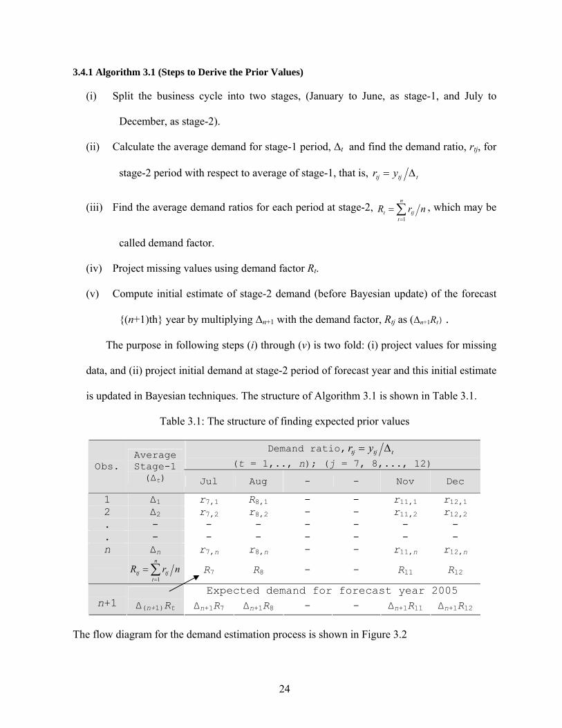
3.4.1 Algorithm 3.1 (Steps to Derive the Prior Values)

(i) Split the business cycle into two stages, (January to June, as stage-1, and July to

December, as stage-2).

(ii) Calculate the average demand for stage-1 period, ∆t and find the demand ratio, rtj, for

stage-2 period with respect to average of stage-1, that is, ttjtj yr ∆=

(iii) Find the average demand ratios for each period at stage-2, ∑=

=n

ttjt nrR

1

, which may be

called demand factor.

(iv) Project missing values using demand factor Rt.

(v) Compute initial estimate of stage-2 demand (before Bayesian update) of the forecast

{(n+1)th} year by multiplying ∆n+1 with the demand factor, Rtj as (∆n+1Rt).

The purpose in following steps (i) through (v) is two fold: (i) project values for missing

data, and (ii) project initial demand at stage-2 period of forecast year and this initial estimate

is updated in Bayesian techniques. The structure of Algorithm 3.1 is shown in Table 3.1.

Table 3.1: The structure of finding expected prior values

Demand ratio, ttjtj yr ∆=

(t = 1,.., n); (j = 7, 8,..., 12) Obs. Average Stage-1 (∆t) Jul Aug - - Nov Dec

1 ∆1 r7,1 R8,1 - - r11,1 r12,1 2 ∆2 r7,2 r8,2 - - r11,2 r12,2 . - - - - - - - . - - - - - - - n ∆n r7,n r8,n - - r11,n r12,n

∑=

=n

ttjtj nrR

1

R7 R8 - - R11 R12

Expected demand for forecast year 2005 n+1

∆(n+1)Rt ∆n+1R7 ∆n+1R8 - - ∆n+1R11 ∆n+1R12

The flow diagram for the demand estimation process is shown in Figure 3.2

25

3.4.2 Bayesian Probability Model (B-P Model)

Following is the structure illustrated in Table 3.1 and Algorithm 3.1, the initial projected

demand for the forecast year (before Bayesian update) is shown in Table 3.2.

Table 3.2: Projected demand averaging the sample data (units in million)

Demand ratio at stage-2 periods (t = 1,.., n); (j = 7, 8,..., 12) Obs. Year

Average Stage-1 (∆t) Jul Aug Sep Oct Nov Dec

1 2000 1.03 2.00 3.01 2.65 2.45 1.61 1.31

. 2001 1.25 1.65 2.56 2.68 2.78 1.73 0.78

. 2002 1.21 1.80 2.49 3.24 2.77 1.99 1.29

(n-1) 2003 1.43 1.41 2.09 3.03 3.95 1.54 1.41

n 2004 1.55 1.53 2.00 3.11 3.57 2.17 1.48

∑=

=n

ttjtj nrR

1

- 1.68 2.43 2.94 3.11 1.81 1.25

Expected demand for forecast year by ∆n+1Rt

(n+1) ∆n+1(=2005) 1.93 3.24 4.69 5.68 5.99 3.49 2.42

Figure 3.2: Flow diagram for Bayesian computation

Input yt, v, t

Compute µ7, µ8, …, µ12 using Equation (3.14)

Use Bayes rule f1(µt|yt) likelihood f(yt|µt)

Prior f0(µt)

Stop

Start

Find conjugate prior distribution f0(µt)

Input data, yt Select probability

density for data

Transform parameters α, β into µ & CV (v)

Calculate CV (v) from past data

26

The parametric values of the prior and posterior distribution for each period at stage-2, under

B-P model are shown in Table 3.3.

Table 3.3: Prior and posterior parameters derived by B-P model for 2005

Prior parameters (units in million)

Posterior parameters (units in million)

Month Mean y CV(v) α β

Estimatedy A B Mean

Jul 1.96 0.16 41.34 79.19 3.24 80.67 206.51 2.59

Aug 2.87 0.13 59.16 167.34 4.69 116.31 435.28 3.77

Sep 3.38 0.28 14.94 47.24 5.68 27.89 120.74 4.49

Oct 3.47 0.42 7.71 23.35 5.99 13.42 57.56 4.63

Nov 2.04 0.34 10.67 19.77 3.49 19.34 49.98 2.72

Dec 1.46 0.33 10.95 14.53 2.42 19.90 36.17 1.91

3.4.3 Sample Calculation (B-P Model)

For the month of July, the mean, Julyy = 1.96, and coefficient of variation, v = 0.16. Using

Equation (3.15b), (3.15c), the value of (α, β) is given by

212 +=

JulJul v

α = 34.41216.01

2 =+ (3.17a)

19.79)134.41(96.1)1( =−=−= αβ JulJul y (million) (3.17b)

For the month of July, the initial estimate, Julyy = 3.24. From Equations (3.16a) and (3.16b),

the parameters of the posterior distribution are determined as:

⎟⎟⎠

⎞⎜⎜⎝

⎛+= Jul

JulJul v

tA α2 67.8034.4116.01

2 =+= (3.18a)

⎟⎟⎠

⎞⎜⎜⎝

⎛+= Jul

Jul

JulJul v

yB β2

ˆ= 5.20619.79

16.024.3

2 =+ (million). (3.18b)

The demand for the month of July in year 2005 is estimated by the parameters (A and B)

of posterior distribution model. The mean of inverse gamma distribution is given by )1( −AB .

27

By using the values Ajul and BJul from Equations (3.18a) and (3.18b), the mean demand for the

month of July is estimated as 59.2)167.80(5.206 =− (million).

3.4.4 Bayesian Probability Model with Incomplete Data (BP-I Model)

Missing data often arise in various settings includes market sales, industrial production,

shipment arrival, new product trials. The forecast based on missing values can often result in

biased and inefficient estimates. In BP-I model, the projections of missing values for stage-2

period in year 2004 and the initial demand estimate for stage-2 period in year 2005 are obtained

by following Algorithm 3.1. The projected missing values and the initial demand for the

forecast year (before Bayesian update) are shown in Table 3.4.

Table 3.4: Projected demand averaging the sample data (units in million)

Stage-2 yt (t=7, 8,. . . ,12) Obs. Year

Average Stage-1 (∆j) Jul Aug Sep Oct Nov Dec

1 2000 1.03 2.00 3.01 2.65 2.45 1.61 1.31

. 2001 1.25 1.65 2.56 2.68 2.78 1.73 0.78

. 2002 1.21 1.80 2.49 3.24 2.77 1.99 1.29

(n-1) 2003 1.43 1.41 2.09 3.03 3.95 1.54 1.41

∑ −

=−= 1

1 )1(n

j tjt nrR - 1.72 2.54 2.90 2.99 1.72 1.20

Expected demand for n-th year by ∆nRt

Projected Missing values

1.55 2.66 3.94 4.50 4.63 2.66 1.86

Actual demand - 2.37 3.09 4.82 5.54 3.36 2.29

(n) (2004)

Percentage error - -0.12% -0.27% 0.07% 0.16% 0.21% 0.19%

(n+1) (2005)

Initial estimate 1.93 3.31 4.90 5.60 5.76 3.31 2.31

The mean demand, coefficient of variation, parameters of the prior model and the

parameters of the posterior model for each period at stage-2 in 2005 under BP-I model are

shown in Table 3.5.

28

Table 3.5: Prior and posterior parameters derived by BP-I model for 2005

Prior parameters (units in million)

Posterior parameters (units in million)

mean CV(v) α β Initial estimate A B Mean

Jul 2.01 0.19 30.26 58.67 3.31 58.52 152.19 2.60

Aug 2.99 0.18 33.69 97.97 4.90 65.38 253.14 3.87

Sep 3.34 0.26 16.58 52.04 5.60 31.15 133.62 4.29

Oct 3.35 0.39 8.65 25.62 5.76 15.29 63.93 4.18

Nov 1.94 0.27 15.63 28.43 3.31 29.26 73.55 2.51

Dec 1.39 0.28 14.34 18.66 2.31 26.69 47.18 1.77

Calculation procedure to obtain the values presented in Table 3.6 is similar to the sample

calculation illustrated in sample calculation under Section 3.3.3. The graphical presentation of

prior and posterior density for both B-P and BP-I models are shown in Figures (A.1 and A.2) in

Appendix A. The results and validation of models are presented in the next section.

3.5 Forecasting Errors and Model Validity

In the forecasting procedure, a portion of the dataset is used to estimate the parameters of

the model; the forecasts are then tested on data to validate the model. In the analysis, data

points for the 7 years (1998-2004) are used to produce the forecasts for the 8th years (at stage-2

from July to December, 2005). To validate the forecasting models, the forecasts are compared

with the original demand for the target forecast periods. The performance of forecasting models

can be achieved by a number of error measure indicators such as relative (percentage) errors

(PEt), mean absolute deviation (MADt) and tracking signal (TSt), where index t corresponds to a

particular period (month). Tracking signal is the cumulative forecast error (running sum) with

respect to MAD for a given time period. It measures the limit of MAD above or below the

actual data. A comparison between B-P model and BP-I model with respect to the percentage

error, mean absolute deviation, and tacking signal are shown in Table 3.6.

29

Table 3.6: PE, MAD, TS for B-P and BP-I models (units in million)

Models Month Forecast

jy Actual

yj

deviation)ˆ( jj yy −

PE

j

jj

yyy |ˆ| −

MADt

nyy jj∑ − |ˆ|

TSt

j

jj

MADyy∑ − |ˆ|

Jul 2.59 2.83 0.24 0.09 0.15 1.65

Aug 3.77 3.33 -0.45 0.13 0.29 -1.50

Sep 4.49 4.10 -0.39 0.09 0.33 -1.18

Oct 4.63 5.11 0.48 0.09 0.36 1.31

Nov 2.73 3.46 0.74 0.21 0.44 1.68

B-P

Dec 1.91 2.28 0.37 0.16 0.43 0.86

Average error = 0.13

Jul 2.60 2.83 0.23 0.08 0.10 2.35

Aug 3.87 3.33 -0.54 0.16 0.32 -1.69

Sep 4.29 4.10 -0.19 0.05 0.28 -0.67

Oct 4.18 5.11 0.93 0.18 0.44 2.11

Nov 2.51 3.46 0.95 0.27 0.54 1.75

Dec 1.77 2.28 0.51 0.22 0.54 0.96

BP-I

Average error = 0.16

The percentage error is computed as |||ˆ| tttt yyyPE −= , mean absolute deviation as

nyyMAD n

t ttt ∑ =−=

1|ˆ| , and tacking signal as t

n

t ttt MADyyTS ∑ =−= 1 )ˆ( . The comparison of

the forecasts derived from B-P and BP-I models with respect to the actual demand is shown in

Figure 3.3.

1000000

2000000

3000000

4000000

5000000

6000000

7

July to December, 2005

Dem

and

quan

tity

B-P modelBP-I modelActual demand

Figure 3.3: Comparison of forecasts with actual demand

30

The projection of the errors by B-P and BP-I models for each forecasted period t, (with j =

7, 8, …, 12) is shown in Figure 3.4. The 13th point represents the average of errors (i.e.,

averaged over all 6-periods).

0.00

0.05

0.10

0.15

0.20

0.25

0.30

0.35

7 8 9 10 11 12 13

July to December, 2005

Perc

enta

ge e

rror

sB-P model

BP-I model

The graphical presentation of tracking signals (TS) of the forecasting models over the test

periods is presented in Figure 3.5.

-3.00

-2.00

-1.00

0.00

1.00

2.00

3.00

7 8 9 10 11 12

July to December, 2005

Trac

king

sig

nals

B-P modelBP-I model

Figure 3.5: Summaries of tracking signals of the models

Figure 3.4: Error comparison of all models

31

3.6 Summary

This model is a two-stage demand planning problem, which is particularly useful when the

demand of the product is uncorrelated over the period. In this forecasting model, the demand

process is described by the probability distribution where the distribution parameters are not

known in advance. Based on the maximum likelihood estimate among several heavy tailed

probability distributions, an appropriate distribution model is chosen for the data series. A

conjugate prior model is selected to describe the variation of the demand rate over the periods.

The parameters of the prior distribution are estimated from the data series collected in the past

seasons. The model is further applied to forecast demand with the assumption that the data

series contains missing values.

The original model was divided into two sub-models: Bayesian probability (B-P) model

and Bayesian probability for incomplete data (BP-I) model. For BP-I model, the demand record

at stage-2 (July to December) in 2004 was considered unavailable while forecasts are made for

stage-2 in 2005. Proposition 3.1 was developed to estimate the missing values and the initial

demand forecast. The Bayesian approach was used to update the demand forecasting for the

stage-2 period in year 2005. The tracking signals of the forecast indicated that forecasts do not

produce trends. Forecast errors for both sub-models were compared with respect to actual data

set and it was concluded that B-P model provided better forecast.

32

CHAPTER 4

THE ARIMA APPROACH TO FORECASTING SEASONAL DEMAND

A fundamental element of a supply-chain management is the estimation of future demand.

This model is specific to forecast seasonal demand from a time series where the demand of a

period is correlated with the demand of the other periods in a business cycle. For example, the

first month demand of a seasonal product during an active demand season indicates the

progression about the future demand of the other period in that season. To forecast such

demand, mathematical models such as autoregressive, moving average, exponential smoothing

techniques are used to predict the future values by extrapolating the known data points. The

autoregressive integrated moving average (ARIMA) procedure is the most sophisticated

forecasting method in time series context (Pankratz, 1983; Vandaele, 1983). The focus of this

chapter is to develop an ARIMA model to forecast the demand of a seasonal product.

The ARIMA is a type of time series forecasting technique developed by Box and Jenkins

(1970), where the autoregressive (AR) and moving average (MA) terms are used to forecast the

demand. To develop an ARIMA model, a sufficiently large dataset is required. The dataset

used in this model is an actual time series demand data of a seasonal product collected from US

census bureau (Table A.1, Appendix A). Two sub-models are studied based on ARIMA theory

to forecast the demand: (a) Fundamental ARIMA (F-ARIMA) and (b) Bayesian sampling-based

ARIMA (BS-ARIMA). The monthly data from January 1996 through June 2005 is used to

construct the model, and forecasts are made for stage-2 period (July to December) in 2005.

A Bayesian approach in the ARIMA model is studied to forecast demand from an

incomplete data series. The model is developed with the assumption that among ninety data

points, six values at stage-2 period (July to December) in 2004 are unavailable. Forecasts are

33

made for stage-2 period in 2005. The main reason for developing BS-ARIMA is to enhance the

model capacity to forecast demand from a data series that contains missing values. A number of

non-informative prior distributions are used to represent the uncertainty of the parameters of

ARIMA model. A Markov chain Monte Carlo sampling algorithm is used to derive the

posterior values of model parameters. In the following sections, the fundamental of classic

ARIMA model is explained first. After identifying the time series pattern, the parameters of

ARIMA model are estimated and applied to forecast demand of the seasonal product.

4.1 Fundamental of the ARIMA Approach (F-ARIMA)

A time series is a set of values (observations) represented by a linear combination of

independent random variable, yt (t = 1, 2, ..., n), where index t indicates the intervals of time.

For seasonal time series data, the direct scale of time is not always necessary to develop the

model. Any mean difference of the series or logarithmic transformation of data can be used to

develop the model. The development of the model involves two basic tasks: (a) identifying the

nature of the demand represented by the sequence of observations, and (b) predicting future

demands of the time series. To achieve the first goal, the following are the steps considered:

♦ first, identify the pattern of observed time series data,

♦ once the pattern is identified, a model is required to interpret the data, and,

♦ then, the parameters of the model are estimated.

The second goal is achieved by extrapolating the model to predict the future demand. In a given

time series the following can be recognized as:

♦ a long-term component of variability termed as trend represents the pattern of the series,

♦ a short-term component, whose shape occurs periodically (at intervals of s lags of the

index variable), is known as seasonality,

34

♦ an autoregressive component of p order, AR(p) relates each value Zt =Yt – (trend and

seasonality) to the (p) previous Z values, according to following linear relationship

tptpttt ZZZZ εφφφ ++⋅⋅⋅++= −−− 2211 (4.1)

where iφ (i =1, …, p) are parameters to be estimated and tε is a residual term; and,

♦ a moving average component of q order, MA(q) relates each Zt value to the q residuals of

the (q) previous Z estimates

qtqttttZ −−− +++−= εθεθεθε ...2211 (4.2)

where iθ (i = 1, 2, …, q) are parameters to be estimated.

The theory of time-series analysis has been developed as a set of linear operators.

According to Box and Jenkins (1970), a highly useful operator in time-series theory is the lag

or backshift linear operator (B) to eliminate the linear or seasonal trend.

4.1.1 Difference Operator to Eliminate Increasing Trend

In time-series analysis, the lag or backshift linear operator (B) is used to eliminate the

linear trend. If the operator B makes 1−= tt ZBZ , which shifts backward in time by one period,

B is called the 1st order delay operator. For example, BZ50 = Z49. The double application of lag

operator is indicated by B2. Applying the lag operator twice to a series, the result is given by

21)( −− == ttt ZBZBZB .

Definition 4.1: The k-th order delay operator is defined as kttk ZZB −= .

Therefore, any integer k is written as kttk ZZB −= . For example, B12Z50 = Z50-12 = Z38.

Using the back operator from Definition 1, the Equation (4.1) can be rewritten as

ttptpttt ZBZZZZ )(2211 φεφφφ ==−⋅⋅⋅−−− −−− (4.3)

where )(Bφ is the autoregressive operator of p order defined by

35

PpBBBB φφφφ −⋅⋅⋅−−−= 2

211)(

Similarly, Equation (4.2) can be written as

tqtqtttt BZ εθεθεθεθε )(2211 =−⋅⋅⋅−−−= −−− (4.4)

where )(Bθ indicates the moving average operator of q order defined by

qqBBBB θθθθ −⋅⋅⋅−−−= 2

211)( .

The autoregressive and moving average components can be combined in an autoregressive

moving average (ARMA) (p, q) model as

qtqtttptpttt ZZZZ −−−−−− −⋅⋅⋅−−−++⋅⋅⋅++= εθεθεθεφφφ 22112211

The lag operator used in the above equation is

tq

qtp

p BBBZBBB εθθθθθθ )1()1( 221

221 −⋅⋅⋅−−−=−⋅⋅⋅−−−

Finally, tt BZB εθφ )()( = . (4.5)

Once linear trends of time series are removed, the periodic trends are eliminated as following.

4.1.2 Periodic Difference Operator to Eliminate Periodic Increase

The analysis of a series begins by evaluating the long and short-term periodic components,

which are essential to define the regular structure of the series. The trend components are

evaluated by fitting a (regular, a polynomial, or a more complicated general) function.

According to Box and Jenkins (1970), the seasonal component is estimated by a seasonal

decomposition procedure, which calculates a seasonal index based on the ratio of the observed

values to the moving average. In the final stage of series modeling, both the trend and the

seasonal component are integrated in the ARMA (p, q) process. For the trend, such integration

is obtained by using the difference linear operator )1( B−=∇ , therefore

tt YBY )1( −=∇ .

36

Definition 4.2: A single application of the ∇ operator transforms the data to a linearly

increasing trend, and repeated use of the ∇ operator for d times )( d∇ transforms the trend to

stationary which can be fitted by a d-order polynomial.

Stationary series Zt obtained after the dth difference )( d∇ of Yt, which is given by

td

td

t YBYZ )1( −=∇= . (4.6)

The combination of ∇ operator in Equation (4.6) and the ARMA (p, q) process results in

an ARIMA (p, d, q) model. Again, ARIMA can be used for the seasonal component of s lag

period, by using both correlations between Zt and Zt-s values and those between the

corresponding residuals εt and εt-s. A seasonal ARIMA model is an ARIMA (p, d, q) model

whose residuals εt are further modeled by an ARIMA (P, D, Q)s. The operators of a seasonal

ARIMA model is defined as (p, d, q)x(P,D,Q)s. ARIMA procedure is expressed as follows:

♦ the non-seasonal autoregressive operator of p order, AR(p) is

ppp BBBB φφφφ −−−−= ...1)( 2

21 ,

♦ the seasonal autoregressive operator of P order, AR(P) is

PLsP

Ls

Ls

sP BBBB ,

2,2,1 ...1)( φφφφ −−−−= ,

♦ the non-seasonal moving average operator of q order, MA(q) is

qq BBBB θθθθ −−−−= ...1)( 2

21 ,

♦ the seasonal moving average operator of Q order, MA(Q) is

QssQ

ss

ss

sQ BBBB ,

2,2,1 ...1)( θθθθ −−−−= ,

and difference operator of d order, dd B)1( −=∇ .

The autoregressive term is determined based on autocorrelation and partial autocorrelation

statistics. The trend of a time series is converted to stationary by the differencing of the data.

37

4.2 Application of Box-Jenkins Methodology

The Box-Jenkins methodology defines the strategy for identifying, estimating and

forecasting autoregressive integrated moving average models. The methodology consists of a

three step iterative cycle, (1) model identification, (2) parameter estimation, and (3) application.

The phases of Box-Jenkins methodology to develop ARIMA model in three stages. Following

Makridakis et. el. (1998), the stages of the F-ARIMA model is shown in Table 4.1.

Table 4.1: Steps of F-ARIMA methodology for time series modeling

Data preparation ♦ Transform data to stabilize variance

♦ Difference data to obtain stationary series

Phase I Identification

Model Selection ♦ Examine data, ACF and PACF to identify potential models

Estimating ♦ Estimate parameters ♦ Select best model if p-value of all model parameters are significant

Phase II Estimation and testing

Diagnostics ♦ Check AIC/PAIC of residuals ♦ Are residual normally distributed?

Phase III Application Forecasting ♦ Use model to forecast

The identification consists of using the data to indicate whether the time series can be

described with a moving average model, an autoregressive model, or a mixed autoregressive-

moving average model. Estimation consists of using the data to make inferences about the

parameters that are needed for the identified model and to estimate parameters of the model.

Diagnostic checking involves the examination of residuals from fitted models to indicate the

model inadequacy for the data series.

4.2.1 F-ARIMA Model Identification

ARIMA model is estimated only after transforming the variable for forecasting into a

stationary series. The stationary series is the one whose values vary over time only around a

38

constant mean and constant variance. The stationary of data series after various differencing is

shown in Figure 4.1.

0

1000000

2000000

3000000

4000000

5000000

6000000

0 25 50 75 100 125

Periods

Dem

and

-2000000.0

-1000000.0

0.0

1000000.0

2000000.0

3000000.0

4000000.0

0 20 40 60 80 100 120

Periods

Varia

bles

, 1st

diff

eren

ce

a) Data series with no differencing b) Stationarity after 1st differencing

-4000000

-3000000

-2000000

-1000000

0

1000000

2000000

0 50 100

Periods

Varia

bles

, 12t

h di

ffer

ence

d

-3000000

-2250000

-1500000

-750000

0

750000

1500000

15 35 55 75 95

Periods

1st &

12t

h di

ffer

ence

d

c) Stationarity after (12) differencing d) Stationarity after (1, 12) differencing

Figure (4.1a) indicates a strong (periodic) seasonal pattern and increasing trend. Figure

(4.1b) is the first differenced data series, which appears to be non-stationary. Figure (4.1c) is

the seasonal (12th) differenced data series, which does not show enough stationarity but a

downward trend. Figure (4.1d) shows the stationarity of data series after first and seasonal (1st

and 12th) differencing. Thus, difference of data series (d1,12) of order 2 is sufficient to achieve

Figure 4.1: Time plot of apparel demand data series after differencing

39

stationarity in mean. After differencing the series, the newly constructed variable is Zt, which is

DdDdt BBZ )1()1( −−=∇∇= . Thus, Zt is determined after differencing the data, which is

)()( 13121 −−− −−−= ttttt yyyyZ . (4.7)

The next part of this step is to identify the values of p and q, which are the AR(p) and

MA(q) components for both seasonal and non-seasonal series. In this step, the main analytical

tool is the autocorrelation function (ACF) and partial ACF (PACF), which are used to identify

the internal structure of the analyzed series. To identify the values of p and q, the

autocorrelation and partial autocorrelation coefficients of various orders of Zt are computed.

Both AR(p) and MA(q) are associated with ACF and PACF. The forms of ACF and Partial

ACF with differencing of data series and after first and seasonal differencing of the data series

are shown in Figure 4.2.

-0.20

0.20.40.60.8

1

1 2 3 4 5 6 7 8 9 10 11 12 13 14 15

Lag

AC

F

-2-1.5

-1-0.5

00.5

1

1 3 5 7 9 11 13 15

Lag

AC

F

a) ACF with no differencing b) ACF of differenced data

-0.6-0.4-0.2

00.20.40.60.8

1

1 3 5 7 9 11 13 15

Lag

PAC

F

-0.6-0.4-0.2

00.20.40.60.8

1

1 2 3 4 5 6 7 8 9 10 11 12 13 14 15

Lag

PAC

F

c) PACF with no differencing d) PACF of differenced data

Figure 4.2: ACF and Partial ACF of differenced demand data

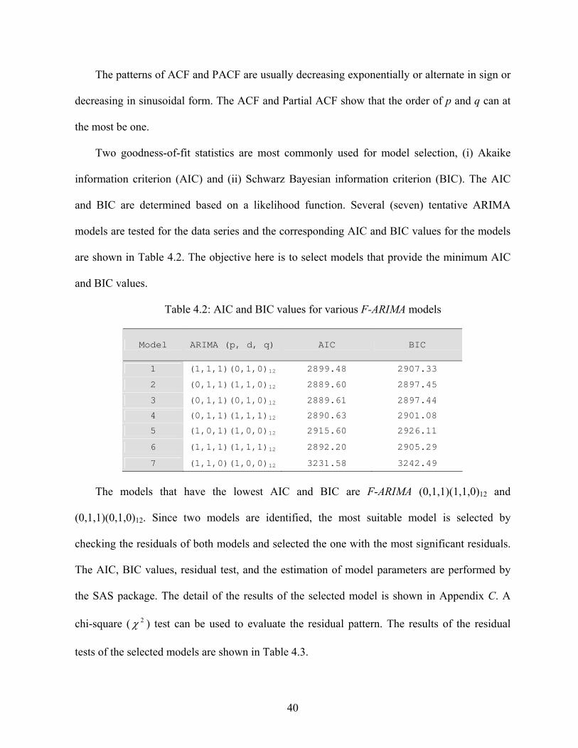
40

The patterns of ACF and PACF are usually decreasing exponentially or alternate in sign or

decreasing in sinusoidal form. The ACF and Partial ACF show that the order of p and q can at

the most be one.

Two goodness-of-fit statistics are most commonly used for model selection, (i) Akaike

information criterion (AIC) and (ii) Schwarz Bayesian information criterion (BIC). The AIC

and BIC are determined based on a likelihood function. Several (seven) tentative ARIMA

models are tested for the data series and the corresponding AIC and BIC values for the models

are shown in Table 4.2. The objective here is to select models that provide the minimum AIC

and BIC values.

Table 4.2: AIC and BIC values for various F-ARIMA models

Model ARIMA (p, d, q) AIC BIC

1 (1,1,1)(0,1,0)12 2899.48 2907.33

2 (0,1,1)(1,1,0)12 2889.60 2897.45

3 (0,1,1)(0,1,0)12 2889.61 2897.44

4 (0,1,1)(1,1,1)12 2890.63 2901.08

5 (1,0,1)(1,0,0)12 2915.60 2926.11

6 (1,1,1)(1,1,1)12 2892.20 2905.29

7 (1,1,0)(1,0,0)12 3231.58 3242.49

The models that have the lowest AIC and BIC are F-ARIMA (0,1,1)(1,1,0)12 and

(0,1,1)(0,1,0)12. Since two models are identified, the most suitable model is selected by

checking the residuals of both models and selected the one with the most significant residuals.

The AIC, BIC values, residual test, and the estimation of model parameters are performed by

the SAS package. The detail of the results of the selected model is shown in Appendix C. A

chi-square ( 2χ ) test can be used to evaluate the residual pattern. The results of the residual

tests of the selected models are shown in Table 4.3.

41

Table 4.3: Autocorrelation check of F-ARIMA residuals

Lag Chi-sq DF Pr > Chi sq. Autocorrelation

ARIMA (0,1,1)(1,1,0)12

6 6.11 4 0.19 -0.066 -0.167 -0.102 -0.125 -0.051 0.003

12 8.53 10 0.58 -0.057 0.089 -0.014 -0.031 0.057 -0.084

18 16.88 16 0.39 0.248 -0.102 -0.01 -0.032 0.003 -0.035

24 29.8 22 0.13 0.026 -0.089 -0.042 -0.199 0.108 0.199

ARIMA (0,1,1)(0,1,0)12

6 8.97 4 0.06 0.126 0.058 -0.133 -0.15 -0.146 -0.057

12 11.81 10 0.30 -0.092 0.046 0.003 -0.014 0.117 0.022

18 26.82 16 0.04 0.237 -0.087 -0.046 -0.213 -0.025 -0.112

24 39.44 22 0.01 -0.066 -0.142 -0.078 -0.175 0.088 0.164

Through examining the autocorrelations and partial autocorrelations and chi-square test of

the residuals in Table 4.3, the results indicates that F-ARIMA (0,1,1)(1,1,0)12 is a significantly

better model. The next step is to estimate the parameters of this model.

4.2.2 Parameters Estimation of F-ARIMA Model

Once a suitable F-ARIMA (p, d, q)×(P, D, Q)12 structure is identified, the second step is the

parameter estimation or fitting stage. The parameters are estimated by the maximum likelihood

method. The results of parameter estimations are reported in Table 4.4.

Table 4.4: Estimated values of the F-ARIMA parameters

Parameter Estimate Standard error t-value Pr>|t| lag

MU 1226.80 7889.10 0.16 0.8700 0

MA1,1 0.74 0.07 10.59 0.0001 1

AR1,1 -0.35 0.09 -3.59 0.0003 12

It is also important to check that the parameters contained in the model are significant. This

ensures that there is no extra parameters are present in the model and the parameters used in the

42

model have significant contribution, which can provide the best forecast. The estimate of

autoregressive and moving average parameters are labeled "MA1,1" and AR1,1, which are

0.735 and -0.35, respectively. Both the moving average and the autoregressive parameters have

significant t values. The subsequent step after the parameter estimation is the Diagnostic

Checking or model verification. The Box and Jenkins (1970) estimation process for seasonal F-

ARIMA model is shown in Figure 4.3.

Data: Time series

Start

Differencing Data sets

Identify order of differencing

Stationarityachieved?

Identify order of AR and MA

Estimate F-ARIMAparameters

Yes

No Further differencing

Demand forecast by F-ARIMA model

Model verified?

YesNo Further model Identification

Build F-ARIMA model

Figure 4.3: Flow chart for F-ARIMA estimation process

43

4.2.3 Diagnostic Checking and Model Validation

The model verification is concerned with checking the residuals of the model to determine

if the model contains any systematic pattern which can be removed to improve on the selected

ARIMA model. Although the selected model may appear to be the best among a number of

models considered, it is also necessary to do diagnostic checking to verify that the model is

adequate. Verification of an ARIMA model is tested (i) by verifying the ACF of residuals using

the chi squared test, (ii) by verifying the normal probability plot of the residuals.

In Table 4.3, it is revealed that there are no significant autocorrelations or any significant

partial autocorrelations of the residuals. The 2χ tests indicated that the hypothesis cannot be

rejected and residuals are uncorrelated. If the residuals are not random, the time series should

be further modeled. Since the model diagnostic tests show that all the parameter estimates are

significant and the residual series do not follow any pattern, it can be concluded that the

ARIMA (0,1,1) (1,1,0)12 model is adequate for the demand series. Therefore, ARIMA (0,1,1)

(1,1,0)12 is used to forecast the demand series.

4.3 Point Forecast with F-ARIMA Model

The ARIMA model (0,1,1) (1,1,0)12 is selected to forecast the demand variable, where

autoregressive term p = 0, P = 1 (seasonal) [that is, )1)(01( 121Bφ−− ]; differencing term d = 1,

D = 1 (seasonal difference) [that is, )1)(1( 12BB −− ] and moving average term q = 1, Q = 0

(seasonal) [ )01)(1( −− Bθ ] . For the dataset in Table A.1, the fitted model is given by

tt eBCyBBB )1( )1( )1( )1( 1212 θφ −+=−−− (4.8a)

Seasonal AR(1)

Non-SeasonalDifference

Seasonal Difference

Non-SeasonalMA(1)

44

The model has (1, 12) period differencing, the autoregressive factors is )1( 12Bφ− = (1 +

0.35096 B12), the moving average factors is )1( Bθ− = (1 - 0.73527 B), and the estimated mean,

C = 1226.8. Transforming autoregressive terms and coefficient, the form of Equation (4.8a) is

given by

)1( )1( )1()1(

1212 BBBeBC

y tt −−−

−+=

φθ

. (4.8b)

After expanding, Equation (4.8b) becomes

)1( )1()1(

131212 BBBBeBC

y tt +−−−

−+=

φθ

)1(

)1( 252413121312 BBBBBBB

eBC t

φφφφθ

−++−+−−−+

= . (4.8c)

Multiplying denominator with left hand side, Equation (4.8d) converts into

ttt eBCBBBBBBByy )1( )( 252413121312 θφφφφ −+=+−−+−+− (4.8d)

Changing the sides Equation (4.8d) yields

CeBBBBBByy ttt +−++−+−++= )1( )])1()1([ 25241312 θφφφφ (4.8e)

Transforming the back operator, the Equation (4.8e) is given by

Ceeyyyyyy tttttttt +−++−+−++= −−−−−− 1252413121 )1()1( θφφφφ . (4.9)

4.4 Forecast Results by F-ARIMA Model

In order to forecast one period ahead, that is, 1+ty , the subscript of the Equation (4.9) is

increased by one unit, throughout, as given by

µθφφφφ +−++−+−++= +−−−−+ tttttttt eeyyyyyy 1242312111 )1()1( (4.10)

The term 1+te is not known because the expected value of future random errors has to be

taken as zero. For the forecast of the second period onward, the term te is also taken as zero as

45

the actual value is not known so the forecast errors can not be found. There are 114 data points

from January 1998 to June 2005 used to build the ARIMA model. Using φ = -0.35 and θ =

0.735, the Equation (4.11) is given by

8.1226735.0 35.035.065.065.0 1242312111 +−+−+−+= +−−−−+ tttttttt eeyyyyyy (4.11)

The results F-ARIMA forecasting model is shown in Table 4.5 (details in Appendix B.1).

Table 4.5: Forecast results by F-ARIMA model (0,1,1)(1,1,0)12 (units in million)

Month Demand Forecast

ActualDemand

Std error

95% lower

95% upper

Jul 2.74 2.83 0.38 1.99 3.50

Aug 3.65 3.33 0.40 2.78 4.34

Sep 4.92 4.10 0.41 4.35 5.96

Oct 5.03 5.11 0.42 5.25 6.91

Nov 2.69 3.46 0.44 2.61 4.31

Dec 2.70 2.28 0.45 1.83 3.58

In order to forecast for the period 115 (that is, July 2005), Equation (4.11) is given by

8.1226ˆ735.0ˆ 35.035.065.065.0 1141159091102103114115 +−+−+−+= eeyyyyyy

The value of 115e is not known, so 115e is replaced by zero. The value for 114e is the

difference of actual demand and the forecasted value for the period 114, which is 1.48.

The forecast quantity for period 115 can be calculated as follows:

115y = 2.32 + (0.65) 2.37 – (0.65) 1.73 + (0.35) 2.02 - (0.35) 1.68 + ( 115e = 0)

+ (-0.73) 1.48 + 0.001

= 2.74 (million).

Predicting demand for the second period forecast, that is, the period 116, the quantity is

116y = 2.83 + (0.65) 3.09 – (0.65) 2.37 + (0.35) 3.0 – (0.35) 2.02+ ( 116e = 0)

+ (-0.73) )0ˆ( 115 =e + 0.001 = 3.65 (million).

46

4.5 Bayesian Sampling-based ARIMA Model (BS-ARIMA)

Bayesian methods have been widely applied in time series context and have played a

significant role in prediction processes. In this section, the Bayesian technique is used in

ARIMA model to forecast demand of a seasonal product within the framework of sampling

theory statistics. The model can be applied in situations where non-standard distributions or

nonlinear regression are more realistic for a given data series, Gamerman (1997). The Markov

Chain Monte Carlo (MCMC) methods is efficient and flexible algorithms for conducting

posterior inference of Bayesian model through simulation. The main reason of using MCMC

methods is to make an inference about analytically intractable parameters of the posterior

model through generating a Markov chain. Depending of the structure of the time series data, a

Markov chain can be constructed in various ways. Gibbs sampler is the most common

algorithm used here to derive the posterior parameters of the model. The application of

Bayesian ARIMA models in time series with complete values is available in Congdon (2003).

The key advantage of developing ARIMA model from Bayesian perspectives is the capacity to

forecast future demand from an incomplete data series that contains both observed and

unobserved data points.

4.5.1 Bayesian Computation at BS-ARIMA Model

A general form of the seasonal ARIMA model is (p,d,q)(P,D,Q)12. For the dataset, the

pattern of the ARIMA model identified in the previous sections has the form (0,1,1)(0,1,1)12. In

Equation (4.9), the ARIMA model has expressed with the form as

Ceeyyyyyy tttttttt +−++−++= −−−−−− 12542431321211 θφφφφ

where )1(1 φφ += , )1(2 φφ +−= , and φφφ == 43 .

47

It is noted that the demand for the stage-2 period from July 2004 to December 2004 are not

available. A dummy variable wt is added to Equation (4.9) to account the missing values of the

data series. The form of the BS-ARIMA after adding dummy variable is given by

ttttttttt wCeeyyyyyy ++−++−++= −−−−−− 12542431321211 θφφφφ . (4.12)

The dummy variable wt, 10 ≤≤ tw is added to represent the status of past information

whether the demand observation is available or not for any period in the past season. A dummy

variable is set to ‘zero’ when demand information of a period is complete. A scaled value of wt

may be set (from 0 to 1) to reflect the partial demand of a period. For example, for a period the

value of wt would be 1.0, if the demand information for the period is unrecorded (missing),

while the value 0.50 indicates incomplete demand information which means approximately

50% of the expected demand was observed due to some unnatural event.

For the data series yt, (t = 1, 2, …, n, n+1, …N), the yt corresponds to the demand of a

period t, where a vector time series from n+1 to N, { }1)( ≥−= nNyF is the prediction periods.

A Bayesian computation is carried out to predict the demand for (N-n) period through the use

of sampling-based algorithm. The particular sampling-based approach used in this model is a

Markov chain Monte Carlo method based on the Gibbs sampler algorithm.

The likelihood function for n observation yt, (y1, y2, …, yn) is denoted by );( ψyf , where

),,,( τβθφψ i= with ) , . . . ,( 41 φφφ =i . The conditional likelihood is then obtained from the

factorization theorem (Zellner, 1996) is given by

),, . . . ,|(. . . ),|()|()|( 11121 ΨΨΨ=Ψ −nnt yyyfyyfyfyf .

Given the prior distribution for Ψ , )|( tyf Ψ , the posterior density for Ψ is given by

)( ).|()|( ΨΨ∝Ψ fyfyf tt .

48

If ) , . . . ,( 1 NnF yyy += , for predicting (N - n) = L period, the predictive density is given by

ΨΨΨ= ∫ dfyyyyf tFtF )().,|()|( , (4.13)

where ),|(∫ ΨtF yy is the density of the future data Fy .

The L steps ahead forecast is then

ΨΨΨΨ=Ψ ∫∫∫ −++++++ dyyyyyyyyyyyf tLnnLntnntntF ),,,|( . . . ),,|( ),|(),|( 11121

To obtain a sample of predictions from the density function in Equation (4.13), for each

tΨ one needs to draw from ),|(∫ ΨtF yy . The following are the steps to predict the future

values of the BS-ARIMA model through Win BUGS.

Step 1: Data Definitions

ty , {for t in (1: n) }

tw , {Dummy (t), for t in 1: N}

Step 2: Model Description

),(~ τµ tt Normaly {for t in (2: n)}

where

tttttttt weeyyyyC βθφφφφµ +++++++= −−−− 1254243132121

21 στ =

Step 3: Assigning Priors

µ ~ Normal (0, 0.001)

iφ ~ Normal(0, 0.001 )

iθ ~ Normal(0, 0.001 )

β ~ Normal(0, 0.001 )

τ ~ Chi-sq (1)

Step 4: Forecasts Period {t = n +1 … N}

],[~ )()( τµ tnewtnew Normaly

ttttttttnew weeyyyyC βθφφφφµ +++++++= −−−− 1254243132121)( {for t in (n +1: N)}

49

It has been shown in Carlin and Gelfand (1990) that the point estimates arising from

),|(∫ ΨtF yy perform well and the variance of this estimated predictive distribution is small.

To complete the model in ‘Step 3’, the following prior distributions are used. The choice of

prior distribution is followed by (Gelman et. al., 2004; Congdon, 2003), where the posterior

models are derived using MCMC approach through WinBUGS package. For the coefficient φ

and θ, the non-informative prior distributions Normal(0, 0.001) are assumed. Parameter β is

expected to follow a relatively informative prior distribution Normal(1.0, 0.1). The precision (a

reciprocal of variance), τ follows a chi squared distribution with one degree of freedom.

To construct the BS-ARIMA, the demand variable yt is placed with all the values observed

from January 1998 to June 2005. An average of stage-1 demand of year 2004 is placed for the

missing period from July to December 2004. For dummy variable wt, the values placed for July

to December 2004 are 0.39, 0.59, 0.63, 0.27, 36, 0.11, respectively; and zeros are placed for the

remainder of the periods of the series. The values for dummy variable for period (July to

December) 2004 are shown in Table 4.6.

Table 4.6: Values of dummy variables for July to December, 2004 (units in million)

Demand Jul Aug Sep Oct Nov Dec

Projected yp 2.54 3.81 4.14 4.05 2.41 1.75

Stage-1 yst-1 1.55 1.55 1.55 1.55 1.55 1.55

Dummy

( )pstt yyw 11 −−= 0.39 0.59 0.63 0.62 0.36 0.11

4.5.2 Forecast Results of BS-ARIMA Model from Incomplete Data

A sampling-based Bayesian approach is adapted to forecast demand from incomplete data

series. The WinBUGS code for demand estimate, parameter estimates and forecast results are

50

shown in Appendix B (B.2 and B.3). The simulation results of the demand forecast for stage-2

period of 2005 with missing observations are shown in Table 4.7.

Table 4.7: Demand Forecast by BS-ARIMA model (units in million)

Month Actual Estimate Std error 2.50% Median 97.50%

Jul 2.83 2.47 0.71 1.07 2.46 3.88

Aug 3.33 3.62 0.73 2.19 3.61 5.07

Sep 4.10 4.77 0.74 3.32 4.76 6.22

Oct 5.31 5.29 0.73 3.89 5.28 6.76

Nov 3.46 4.28 0.77 2.75 4.28 5.76

Dec 2.28 2.97 0.77 1.53 2.96 4.50

4.6 Forecast Using Adaptive Exponential Smoothing Technique

In this section, an adaptive approaches of Holt-Winters’ (H-W) exponential smoothing

technique is presented to forecast the seasonal demand. For trend and seasonal data, the

multiplicative exponential smoothing (M-ES) model is commonly used in forecasting. The

purpose to study this model is to compare the performances of other forecasting models.

Forecasting demand for the next T periods using M-ES model, the time series is represented by

the model, Askin and Goldberg (2002), Gardner (2006)

( ) LTtttTt SGTRy −+−−+ += 11 ,

where tR is the estimate of level index, tG is the estimate of the trend, and tS is the estimate of

seasonal component (seasonal index). The parameters are estimated as following.

(i) The overall smoothing of level index tR is

( )11 )1( −−−

+−+= ttLt

tt GR

Sy

R αα ,

where 0 < α < 1 is a smoothing constant.

51

(ii) The smoothing of the trend factor tG is

( ) 11 )1( −− −+−= tttt GRRG ββ ,

where 0 < β < 1 is a second smoothing constant.

(iii) The smoothing of the seasonal index tS is

Ltt

tt S

Ry

S −−+= )1( γγ ,

where 0 < γ < 1 is the third smoothing constant.

The initial values of the parameters α, β, and γ are determined using the data from July

2002 to December 2002. The values are modified in subsequent years. The criterion used for

selecting the initial values of the parameters is the value that provides the minimum mean

absolute percentage error (MAPE) of the test dataset. The data series from January 2003 to

June 2005 are used to adjust the weight of the smoothing parameters and demand forecast is

performed for the stage-2 (July to December) in 2005. The demand is estimated using the most

recent demand observation yt, the seasonal factors, and the level index estimates of the time

series. The numerical illustration to forecast stage-2 (July to December) in 2005 is shown in

Appendix B.4. The estimates and actual demand for stage-2 in year 2005 by M-ES model are

shown in Table 4.8.

Table 4.8: Forecast results by M-ES model (units in million)

Month Seasonal Factor Level Trend Forecast Actual Error

St Rt Gt ty yt

Jul 0.95 3.02 0.04 2.90 2.83 -0.06

Aug 1.24 2.99 0.03 3.74 3.33 -0.42

Sep 1.75 2.88 0.02 5.07 4.10 -0.97

Oct 2.15 2.82 0.01 6.08 5.31 -0.77

Nov 1.14 2.87 0.01 3.29 3.46 0.17

Dec 0.84 2.85 0.01 2.40 2.28 -0.12

52

4.7 Forecast Performance and Model Validation

To evaluate the forecasting ability of the models, a number of assessment tools are used to

measure the forecast accuracy. Performance measure indicators, such as relative or percentage

errors (PE), the mean absolute deviation (MAD), relative error, tracking signals (TS) are used to

test the model performances. The equations to calculate relative errors, the mean absolute

deviation, and Tracking Signal of the forecasts are shown in Chapter 3 from Equation (3.15) to

(3.18). The measures of the forecasting models are shown in Table 4.9.

Table 4.9: Forecast by F-ARIMA, BS-ARIMA and M-ES models (units in million)

Model Month Forecast

jy Actual

yj

deviation)ˆ( jj yy −

PE

j

jj

yyy |ˆ| −

MADt

nyy jj∑ − |ˆ|

TSt

j

jj

MADyy∑ − |ˆ|

Jul 2.74 2.83 0.01 0.03 0.09 1.00Aug 3.65 3.33 -0.32 0.10 0.21 -0.64Sep 4.92 4.10 -0.82 0.20 0.34 -0.42Oct 5.03 5.11 0.08 0.02 0.11 1.27Nov 2.69 3.46 0.77 0.22 0.18 0.23Dec 2.70 2.28 -0.42 0.19 0.10 -0.24

F-ARIMA

Average = 0.13

Jul 2.23 2.83 0.60 0.21 0.60 1.00Aug 3.27 3.33 0.06 0.02 0.33 0.18Sep 3.95 4.10 0.15 0.04 0.27 0.56Oct 4.47 5.11 0.64 0.13 0.36 1.77Nov 3.47 3.46 -0.004 0.002 0.29 -0.02Dec 2.32 2.28 -0.003 0.02 0.25 -0.17

BS-ARIMA

Average = 0.067

Jul 2.90 2.83 -0.06 0.02 0.06 -1.00Aug 3.74 3.33 -0.42 0.12 0.24 -1.73Sep 5.07 4.10 -0.97 0.24 0.48 -2.01Oct 6.08 5.11 -0.97 0.19 0.61 -1.61Nov 3.29 3.46 0.17 0.05 0.52 0.32Dec 2.40 2.28 -0.12 0.05 0.45 -0.27

M-ES

Average = 0.11

The graphical presentations of the demand forecast derived by the F-ARIMA, BS-ARIMA

and M-ES models with respect to the actual demand are shown in Figure 4.4.

53

1000000

2000000

3000000

4000000

5000000

6000000

7000000

7 8 9 10 11 12

July to December, 2005

Dem

and

quan

tity

ActualF-ARIMABS-AIRMAM-ES

Figure 4.4: Comparison of forecast and actual demand

Tracking Signal (TS) is an indicator if the forecast follows any trend that needs to be

adjusted. The graphical presentations of the tracking signals fluctuation of the both models are

shown in Figure 4.5.

-3.50

-2.50

-1.50

-0.50

0.50

1.50

2.50

3.50

7 8 9 10 11 12

July to December, 2005

Trac

king

Sig

nals

F-ARIMABS-ARIMAM-ES

Figure 4.5: Tracking signal of the F-ARIMA, BS-ARIMA and M-ES models

4.8 Summary

In this chapter an ARIMA approach is used to forecast the demand of a seasonal product. It

is possible to explore a number of interrelated models where the demand process is correlated

across time. Based on the demand pattern, the F-ARIMA (0,1,1) (1,1,0)12 model was found to

54

be the best fit model for the dataset. For a non stationary stochastic time series such as winter

apparel, the forecasting model often becomes complicated. In ARIMA model, forecast errors

are incorporated to refine the predicted value, so the model gradually improves toward the end

of the time series and provides satisfactory forecasting accuracy.

There are major advantages of using Bayesian methodology to forecast non-stationary

demands. As classical ARIMA requires significantly long data series, a Bayesian-sampling

based ARIMA model was proposed to model from smaller data or incomplete data with

missing values. In this sub-model, it is assumed that data points at stage-2 (July to December)

in 2004 were unavailable. A number of non-informative priors were used for the model

parameters (α, β, τ). The posterior values of the parameters were computed numerically using

the Markov Chain Monte Carlo (MCMC) simulation and BUGS/WinBUGS software.

A multiplicative approach of exponential smoothing (M-ES) technique is considered as the

base reference to forecast seasonal demand and used to measure the forecast performances of

the other models developed in the study. Both time series forecasting models and M-ES models

are used to forecast the demand for stage-2 period in 2005. Test results of the ARIMA (F-

ARIMA and BS-ARIMA) and M-ES models showed that both approaches have the advantages of

easy modeling and significant accuracy. Errors were less than 13% for all models. Checking the

tracking signals of the models, it is found that M-ES model has negative trends, which specifies

that demand forecast made by M-ES model is larger with respect to actual demand. Therefore,

the ARIMA models are appropriate for seasonal forecast and the Bayesian ARIMA model is

advantageous of the all forecasting models.

55

CHAPTER 5

INVENTORY COST REDUCTION USING IMPROVED FORECASTING

In a supply chain, the random occurrences of demand are studied to manage the inventory

system and the planned customer service at minimum costs. Inventory of a product may stock-

out or over-stock if actual demand mismatches the demand forecast. If inventory quantity is

determined based on improved forecast, the inventory cost of a product may be reduced. The

focus of this chapter is to demonstrate the inventory cost reductions through the application of

an appropriate demand forecast of a seasonal product during an active demand season. The best

forecast for the product may be selected by comparing the inventory costs derived from several

forecasts. The inventory policies are applied to the actual data series and the demand forecasts

derived previously.

5.1 Model Description

The inventory policies are used to determine the inventory quantity of a seasonal product

for an active demand season. The study has two objectives: (a) to demonstrate the reduction of

inventory cost due to improved forecasts, and (b) to determine the procurement quantity of the

products to maintain a satisfactory customer service level. A newsvendor inventory model with

emergency procurement option is used to determine the inventory quantity. A dynamic

programming (DP) algorithm is used to determine the inventory costs of actual demand and the

demand forecast. A periodic review policy is used as a model to compare the cost determined

by the extended newsvendor model. After applying these inventory policies to the actual

demand data, the same inventory policies are applied to each forecast. The percentage above

the inventory cost of a forecast, with respect to the inventory cost of actual demand, provides a

basis to compare the forecasting models. The demand forecast that provides the minimum

56

percentage is considered as the appropriate forecast for the active demand period. Thus, this

chapter presents the cost savings approach in the inventory of a seasonal product by combining

the improved forecasting technique and the appropriate inventory policy. The steps to compare

the forecasting models are described as follows.

5.2 Procedure to Compute Optimal Inventory Cost

The following are the steps to compute the optimal inventory costs and the relative

improvement measures of the forecasting models:

Step 1: Find customer service level by specifying the probability (P1) of no stock-out

from two inventory policies: (a) customer service level using newsvendor model with

emergency replenishment policy, and (b) periodic review policy.

Step 2: Select the safety factor z to satisfy P(Z) = (1- P1).

The value of unit normal variable, P(Z) (with mean 0, standard deviation 1) may be

obtained from Z-table or from inverse function of normal distribution.

Step 3: Determine the ordering quantity, Q, from the forecast during lead time L ( Ly ) and

the safety stock (SS). The safety stock is calculated from standard deviation of the

forecast error, SS = ZσL. Therefore, the ordering quantity is

LL ZyQ σ+= ˆ .

Ordering quantity may be increased to the next higher integer.

Step 4: Compute the optimal inventory cost of actual demand and demand forecasts using

dynamic programming (DP) algorithm. Then, calculate the relative cost of each

demand forecast with respect to the cost derived from actual demand.

Step 5: Choose the best forecasting model that gives the minimum costs.

57

5.3 Cost Components to Determine the Customer Service Level

Businesses often face leadtime delay (shipment time) and cost factors such as

transportation cost, set-up costs while procuring products. Inventory is managed to meet

demand and maintain relatively low inventory cost during an active selling season. In inventory

system, a customer service level is specified as the probability (P1) of no stock-out during the

active demand period. It is assumed that the procurement leadtime is one month. To determine

the customer service level, the following is the cost components assumed for the time series.

The inventory cost and variable cost per unit per period (holding cost, setup cost, shortage costs

etc.) are listed in Table 5.1. The holding cost rate is 30% per year. Therefore, holding cost ht

per month is, ht = ($25)(0.30/year)/(12 months/year) = $0.624/month.

Table 5.1: Unit costs applied to the inventory model

Parameters Jul Aug Sep Oct Nov Dec

Dt Actual Demand (in million, $) 2.87 4.33 5.30 5.46 3.41 2.49

At Fixed cost

(in thousand, $) 15.0 14.0 16.0 16.0 17.0 19.0

ct variable cost ($) 25.0 25.0 24.0 25.0 26.0 30.0

πt shortage cost ($) 5.0 5.0 5.0 5.0 5.0 5.0

ht inventory cost ($) 0.624 0.624 0.624 0.624 0.624 0.624

A newsvendor inventory model with a provision for an urgent shipment is used to

demonstrate the customer service level. A general periodic review model is also used as an

alternate inventory policy to determine the inventory quantity and cost to compare the extended

newsvendor model.

5.4 Newsvendor Procurement Model

In a newsvendor model, if the demand is in excess to the inventory level, then the sales are

lost, while, if too much is ordered, inventory remains at the end. To reduce the lost sales, an

58

urgent procurement option is included in the basic newsvendor model. In this model, two types

of procurement approaches are considered: (i) standard procurement at regular interval, (ii)

urgent (emergency) procurement if shortages occur during the peak selling period.

Products are ordered for a peak season (stage-2) at a variable ordering cost of c per item.

For quantity yt, the total procurement cost C1 is cyt . Inventory carrying cost occurs when

procurement quantities yt are more than actual demand xt ( tt xy > ). For a unit inventory holding

cost of h, the total inventory cost C2 is

C2 = ∫ −ty

tttt dxxfxyh0

)()( , if tt xy > .

5.4.1 Expedite Cost Factors

Two additional costs factors are associated with an urgent procurement process: (i) urgent

shipping cost, b1, and (ii) cost due to buyers’ waiting time, b2. The leadtime for urgent shipment

is denoted as τ, which may be considered as a decision variable. When yt is less than the actual

demand, a cost factor, ( 11 ≥b ) is multiplied with the unit purchasing cost c due to emergency

(fast) shipment. The urgent shipment cost, b1c may be expressed as function of the urgent

leadtime τ as τcb1 . For any demand above yt, the urgent shipment cost, C3, is given by

∫∞

−=ty

tttt dxxfyxcbC )()(13 τ , if tt yx > . (5.1)

In the urgent procurement process, another cost factor, (b2>1) is assigned due to buyers’

waiting time cost during the urgent shipment leadtime. The shorter waiting time reduces the

buyers’ waiting time cost, so the leadtime τ is inversely proportional to the cost, which is

expressed as τcb2 . For any demand above yt, the buyers’ waiting time cost at stage-2, C4 is

given by

59

∫∞

−=ty

tttt dxxfyxcbC )()(24 τ

, if tt yx > . (5.2)

5.4.2 Urgent Leadtime Cost Function

The urgent transportation cost and the buyers’ waiting time costs are a function of urgent

procurement lead time τ. By combining the above costs from Equation (5.1) and (5.2), the costs

regarding the urgent procurement response, u(τ) , are

( )τττ /)( 21 bbcu += . (5.3)

A property regarding the urgent shipment function )(τu implies that the leadtime τ can be

reduced by increasing the shipment cost through expedite shipment process. Thus, the buyers’

waiting-time costs can be reduced. The urgent procurement leadtime, )(τu , is a convex cost

function and holds an optimum value for τ >0. Thus, the value for the urgent shipping leadtime

τ can be obtained by setting 0)( =ττ ddu as

12* bb=τ . (5.4)

In Equation (5.4), the optimal leadtime τ* decreased if urgent shipment cost factor b1 is

increased, or the buyers’ waiting cost factor b2 decreases. Substituting the value τ* from

Equation (5.4) into Equation (5.3) yields

⎥⎦⎤

⎢⎣⎡ += *

2*1

*)(τ

ττ bbcu⎥⎥⎦

⎤

⎢⎢⎣

⎡+=

12

2121 bb

bbbbc 212 bbc= . (5.5)

Property 5.1: From Equation (5.5), it is implied that if shortages occur during active demand

season at stage-2, the unit price of the product with urgent procurement process increases at

least twice the original unit cost.

Proof (Property 5.1): If the urgent shipment cost factor b1 and the buyers’ waiting cost factor b2

are set to 1, i.e., b1 = b2 = 1, then Equation (5.5) becomes

60

ccbbcu 21.122)( 21 ===τ ,

which is equivalent to two times of the product purchasing cost.

5.4.3 Cost Minimization in Newsvendor Model

The total cost function includes regular procurement costs (C1), inventory costs (C2), and

urgent procurement costs that includes urgent shipment cost (C3) and leadtime waiting costs

(C4), the total cost is

=),( τtyTC C1 + C2 + C3 + C4. or,

tttty y

tttt

y

tttttt dxxfyxcb

dxxfyxcbdxxfxyhcyyTCt t

t

)()()()()()(.),( 21

0

−+−+−+= ∫ ∫∫∞ ∞

τττ (5.6a)

ty

ttt

y

tttttt dxxfyxudxxfxyhcyyTCt

t

∫∫∞

−+−+= )())(()()(.),(0

ττ , (5.6b)

where, ⎥⎦⎤

⎢⎣⎡ +=

τττ 2

1)( bbcu .

Proposition 5.1: )( tyTC is a convex function.

Proof (Proposition 5.1): Taking the first order derivatives with respect to yt, Equation (5.6b)

gives

∫∫∞

−+=t

t

ytt

y

ttt

dxxfudxxfhcdy

dTC )(.)()(0

τ , (5.7)

[ ])(1)()( ii yFuyhFc −−+= τ .

The second order derivatives of Equation (5.6b), with respect to Q gives

[ ])()()(2

2

iii

yfuyhfdy

TCd τ+= ,

[ ])()( τuhyf t += . (5.8)

61

From Equation (5.8), u(τ) is positive, and inventory holding cost h is a positive quantity.

Therefore, ( 22tdyTCd > 0) is positive. Thus, )( tyTC is a convex function.

Since TC(yt) is a convex function, an optimal yt* for stage-2 exists.

Now, setting 0=dydTC yields

[ ] 0)(1)()( * =−−+ tt yFuyhFc τ , (5.9)

or, hucuyF t +

−= ∗

∗

)()()(

ττ . (5.10)

Substituting 21* 2)( bbcu =τ gives

⎥⎥⎦

⎤

⎢⎢⎣

⎡

+

−=

hbbccbbc

yF t21

21

22

)( . (5.11)

5.4.4 Numerical Example (Newsvendor Inventory Policy)

The unit price of a seasonal product ($c) in a distributor’s store during stage-2 (July to

December) in 2005 is arbitrarily set to $25.00 and holding cost rate is 15% per year. The

possibilities of stock-out during peak sale period may prompt the manager to arrange for an

urgent procurement of the product. The estimated cost for urgent procurement is extra $5 and

the waiting cost for end market buyers is $5 when shortages occur. The holding cost (6-months

season) Season./313.0$year/months 21

year/15.0)month 1)(0.25($ ==h Costs components using c =

$25.0/per unit, b1 = $5.0/per unit, and b2 = $5.0/per unit. The customer service level based on

demand forecast during peak season may be obtained from Equation (5.11),

F(y) hbbc

cbbc

+

−=

21

21

2

290.0

313.0)5)(5()25)(2(25)5)(5()25)(2(

=+−

=

Hence, the customer service level as 90% during the busy demand period.

62

5.5 Alternate Inventory Policy (Periodic Review)

A periodic review policy is considered as an alternative policy to check the result of

newsvendor model. A monthly review plan is considered for periodic inventory replenishment.

There are t (t = 1, 2, …, n) forecasting periods at stage-2 and the demand forecast at any period

t is yt, while the actual demand for any period is xt. Shortages may occur when tt yx > . The

shortage cost is πt dollars per period. To place an order for procuring yt items, the fixed

ordering cost is A dollars, unit purchasing cost is c dollars and unit holding cost is h dollars.

Each unit brings a price of w dollars when it is sold, where w > c. Average fixed ordering cost

per period is given by A/yt, while revenue earned per period is tycw )( − , and average

inventory per period is 2

)( tt xyh −. In a periodic (yt, L) replenishment policy, the expected

shortages S(yt, L) with respect to actual demand xt is given by

∫∞

−=ty

ttttt dxxfyxLyS )()(),(

[ ])(1)(),(),(

ty

tttt

t yFdxxfLySdy

LydS

t

−−=−== ∫∞

.

The expected shortage cost per replenishment cycle is [ ])(1 tyFL

−π . Aggregating the cost

components, a profit function for a periodic inventory replenishment policy is given by

),( )(2

)( LySLy

AxyhycwzMax tt

tttπ

−−−−−= . (5.12)

Taking the first derivative of Equation (5.16) and setting to zero, the expected profit function is

0),(2

=−−= LySdyd

Lh

dydz

ttt

π

63

or [ ] 0)(12

=−+− tyFL

h π (5.13)

After rearranging, Equation (5.13) gives

π21)( hLyF t −= , (5.14)

where F(yt) is the critical fractile of the demand distribution function. This indicates the

probability of no stock-out (customer service level) during the demand period. Following the

numerical example in Section 5.4.4 and using L= one-month period, A, c, h, and π from Table

5.1, the Equation (5.14) yields 94.0)( =tyF .

The probability of no stock-out (P1) during busy period is 0.94. Therefore, a 94% customer

service level is considered for the periodic review inventory policy.

5.6 Selection of Order Points

In this section, a procedure is discussed to find the order point (inventory replenishment

quantity) for each period during an active demand season. The order point is equal to the

forecast of the demand for the leadtime period and the safety stock. The safety stock is

determined by the standard deviation of the forecast error, σL multiplied by a service factor, Z.

Therefore, safety stock (SS) is given by SS = ZσL .

5.6.1 Obtaining Order Points by Considering Forecast Errors

The service factor Z is determined from the probability of no stock-out per replenishment

cycle. Probability of no stock-out should be no lower than Pi {(i = 1, 2) where P1 is obtained

from newsvendor policy, and P2 is obtained from periodic review policy}. Conversely, the

probability of stock-out should be no more than (1 - Pi). Safety factor is selected from the

customer service level, which is given by

P(Z) = (1- Pi), (i = 1, 2) (5.15)

64

where Pi is the probability of no stock-out. The value of Z from P(Z) is obtained from Z-table.

For example, if P1 is 90%, the value for Z is determined by )1.0(1−Φ from Z-table, which is

1.28. The stock-out probability, Pi and the Z-values corresponding to extended newsvendor and

periodic review policies are shown in Table 5.2.

Table 5.2: Probability of stock out and corresponding safety factor

Inventory models Pi Z

Extended Newsvendor (P1) 90% 1.28

Periodic review (P2) 94% 1.55

Using the forecast ty and the standard deviation of the forecast error, σL during the lead

time period, the order point (Q) is given by

LL ZyQ σ+= ˆ . (5.16)

Considering the forecast generated from (B-P) forecasting model in Chapter 3, the order

point Q using extended newsvendor and periodic review policies is shown in Table 5.3.

Table 5.3: Order points derived by (B-P) forecasting model

Newsvendor Policy

Periodic Review Inventory

Policy

Forecast (million)

yt

Std dev (million)

σL Z Q (million) Z Q

(million)Jul 0.69 0.47 1.28 3.29 1.55 3.42

Aug 3.89 0.47 1.28 4.49 1.55 4.62

Sep 4.74 0.47 1.28 5.35 1.55 5.48

Oct 5.01 0.47 1.28 5.62 1.55 5.74

Nov 2.91 0.47 1.28 3.51 1.55 3.64

Dec 2.01 0.47 1.28 2.62 1.55 2.75

5.6.2 Numerical Illustration (Order Points)

For the month of July, the demand forecast by Bayesian probability (B-P) model, y = 2.69

(million). The standard deviation of the forecast error computed from (B-P) model, σL = 0.47

(million). In newsvendor policy, the value of Z = 1.28. Safety stock is calculated as

65

SS = ZσL = (1.28)( 0.47) = 0.61 (million)

The order point Q for the month of July 2005, using Equation (5.16), is given by

Qjul = LL Zy σ+ˆ = 2.69 + 0.61 = 3.29 (million)

The order quantity for stage-2 demand using the customer service level obtained from

newsvendor policy and periodic review inventory policy are shown in Table 5.4 and Table 5.5,

respectively. The details calculations are shown in Appendix C.1.

Table 5.4: Order quantity for stage-2 by newsvendor policy (units in million)

Forecasting Approach Model Jul Aug Sep Oct Nov Dec

B-P 2.88 4.34 5.31 5.47 3.42 2.50Bayesian Probability

Model BP-I 2.86 4.57 5.17 5.21 3.37 2.50

FARIMA 2.93 4.10 5.49 5.49 3.20 3.19ARIMA Model B-FARIMA 2.88 4.25 5.76 6.45 5.02 3.54

Exponential Smoothing M-ES 3.53 4.80 6.42 7.54 4.46 3.40

Table 5.5: Order quantity for stage-2 by periodic review policy (units in million)

Forecasting Approach Model Jul Aug Sep Oct Nov Dec

B-P 2.92 4.43 5.44 5.57 3.53 2.60Bayesian Probability

Model BP-I 2.89 4.68 5.29 5.33 3.51 2.63

FARIMA 2.97 4.20 5.62 5.59 3.31 3.29ARIMA Model B-FARIMA 2.91 4.33 5.91 6.60 5.19 3.70

Exponential Smoothing M-ES 3.67 5.02 6.70 7.84 4.70 3.61

5.7 Optimal Inventory Cost

In this section, the computations to derive the optimal inventory costs for all demand

forecasts by using dynamic programming (DP) algorithm are discussed. It had been shown in

the work of Wagner-Whitin (1958) that the DP algorithm guarantees the minimum inventory

66

cost, which comprises the cost for replenishment and carrying inventory. This minimum

inventory cost is the optimal cost for inventory. The DP method is based on two main

assumptions. The assumptions are as follows:

(i) The required quantity must be available at the beginning of a period.

(ii) No shortages are allowed

5.7.1 Optimal Inventory Cost Using Dynamic Programming

Suppose, Ft is defined as the total cost of the best replenishment strategy that satisfies the

demand requirements at stage-2 (periods 1, 2, …, t). To illustrate the procedure for finding Ft

and the associated replenishment orders, the forecast obtained by Bayesian probability (B-P)

model is used. The cost components are shown in Table 5.1. A DP algorithm is applied to

determine the inventory quantity and procurement costs, which is shown in Table 5.6.

Table 5.6: Inventory quantity and procurement cost by B-P model (units in million)

Cost of ordering at stage-2, 2005 Fj

Jul Aug Sep Oct Nov Dec

1 71.91* 183.06 322.55 469.58 563.59 633.82

2 180.37* 316.54 460.16 552.03 620.70

3 307.93* 442.66* 528.98* 593.59*

4 444.73 532.34 597.89

5 531.57 598.06

6 603.92

j*(k) 1 2 3 3 3 4

Min 71.91 180.37 307.93 442.66 528.98 593.59

From Table 5.6, the minimum inventory cost over the six-period planning horizon using

demand forecast by the B-P model for stage-2 is $593.59. There are four replenishments during

stage-2. The inventory quantity and time period for replenishment during stage-2 are shown in

Table 5.7.

67

Table 5.7: Inventory quantity and replenishment time for stage-2 (units in million)

Jun Jul Aug Sep Oct Nov Dec

Qt - 3.29 4.49 5.35 5.62 3.51 2.62

Replenishment 1st 2nd 3rd - - 4th -

Qoptimal 3.29 4.49 14.48 - - 2.62 -

In the first and second replenishment, the inventory quantity required for July and August

are 3.29 ×106 and 4.49 ×106, respectively. The third replenishment quantity is 14.48 ×106,

which is the total quantity required for September, October and November. This replenishment

order is placed at the same time (as j*3 = 3, j*

4 = 3, j*5 = 3) at the beginning of August. The

fourth replenishment, j*6 = 4, are placed for the inventory requirement in the month of

December. The order is placed at an amount Q*6 = 2.62 at the beginning of November so that

inventory will be at hand prior to December. The numerical illustration of the results presented

in Table 5.7 is shown in Appendix C.2.

5.7.2 Determining Inventory Costs for All Forecasts

In this section, the average inventory costs per period are determined for each inventory

policies using the dynamic programming method. The procedure to calculate inventory cost is

described in Section 5.5.2. The cumulative inventory costs based on the quantity required per

period for stage-2 period (from July to December) in 2005 implementing newsvendor inventory

policy is shown in Table 5.8. In this table, the minimum inventory costs for each period for

each of the demand forecasts are shown. The number of replenishment orders for stage-2

period and the corresponding replenishment placement time based on newsvendor inventory

policy is shown in Table 5.9. A sample computation of inventory costs and replenishment order

placement arrangement is shown in Table 5.6 and 5.7, respectively. The minimum inventory

68

cost for each period, replenishment orders and correspond time period for each demand

forecasting method are presented in Appendix C.3.

Table 5.8: Inventory cost using newsvendor policy for stage-2, 2005

Inventory Cost for stage-2 period, 2005 Forecasting Approach Model

Jul Aug Sep Oct Nov Dec

B-P 71.91 180.37 307.93 442.66 528.98 593.59Bayesian Probability

Model BP-I 86.84 206.46 334.67 467.14 554.66 622.14

F-ARIMA 86.12 194.96 329.91 470.94 556.56 644.62ARIMA Models BS-ARIMA 65.66 157.28 261.57 381.29 478.75 549.01

Exponential Smoothing M-ES 87.95 197.03 333.68 498.75 597.51 675.71

Table 5.9: Inventory quantity by newsvendor policy at stage-2, 2005 (units in million)

Model - Jul Aug Sep Oct Nov Dec

Q 3.29 4.49 5.35 5.62 3.51 2.62

j*(k) 1st 2nd 3rd - 4th - - B-P

Qrep 3.29 4.49 14.48 - 2.62 - -

Q 3.47 4.78 5.34 5.38 3.47 2.61

j*(k) 1st 2nd 3rd - - - - BP-I

Qrep 3.47 4.78 16.80 - - - -

Q 3.44 4.35 5.62 5.73 3.39 3.40

j*(k) 1st 2nd 3rd - - - - FARIMA

Qrep 3.44 4.35 18.14 - - - -

Q 2.63 3.66 4.34 4.86 3.86 2.72

j*(k) 1st 2nd 3rd - - - - B-FARIMA

Qrep 2.63 3.66 15.78 - - - -

Q 3.52 4.36 5.69 6.70 3.91 3.02

j*(k) 1st 2nd 3rd - - - - M-ES

Qrep 3.52 4.36 19.33 - - - -

The optimal inventory costs using periodic review inventory policy and the replenishment

costs per period at stage-2 are shown in Table 5.10. The number of replenishment orders for

stage-2 period and the corresponding replenishment order placement using periodic review

inventory policy is shown in Table 5.11. Detail computation results, optimal inventory cost,

replenishment time period for each demand forecast are presented in Appendix C.4.

69

Table 5.10: Inventory cost based on periodic review inventory policy

Inventory Cost for stage-2 period, 2005 Forecasting Approach Model

Jul Aug Sep Oct Nov Dec

B-P 85.59 201.14 332.59 474.04 566.01 637.15Bayesian Probability

Model BP-I 90.72 214.24 346.18 482.49 573.94 645.44

F-ARIMA 89.81 202.36 340.85 485.52 574.87 666.75ARIMA Models BS-ARIMA 82.00 192.54 328.45 484.18 606.30 693.60

Exponential Smoothing M-ES 91.21 203.56 343.34 511.62 613.68 695.26

Table 5.11: Inventory quantity by periodic review at stage-2, 2005 (units in million)

Model - Jul Aug Sep Oct Nov Dec

Q 3.42 4.62 5.48 5.74 3.64 2.75

j*(k) 1st 2nd 3rd - - - - B-P

Qrep 3.42 4.62 17.61 - - - -

Q 3.63 4.94 5.50 5.54 3.62 2.76

j*(k) 1st 2nd 3rd - - - - BP-I

Qrep 3.63 4.94 17.42 - - - -

Q 3.59 4.50 5.77 5.88 3.54 3.55

j*(k) 1st 2nd 3rd - - - - F-ARIMA

Qrep 3.59 4.50 18.74 - - - -

Q 2.71 3.75 4.43 4.95 3.94 2.80

j*(k) 1st 2nd 3rd - - - - B-FARIMA

Qrep 2.71 3.75 16.12 - - - -

Q 3.65 4.49 5.82 6.83 4.04 3.15

j*(k) 1st 2nd 3rd - - - - M-ES

Qrep 3.65 4.49 19.85 - - - -

5.8 Comparison of Forecasting Methods

In this section, the forecasting models are compared based on total inventory cost (TIC),

mean absolute percent error (MAPE) and standard deviation of the forecast error. The average

inventory costs are determined for actual demand data and each demand forecast using the

extended newsvendor model and a periodic review model for an active demand season. The

inventory cost associated with actual demand is the least inventory cost, which is considered

the base cost reference to the demand forecasts. The relative percent of inventory cost (RPIC)

70

for each forecast is then determined. These percentages are compared and the minimum

percentage value is considered the appropriate forecast for the demand data series. The standard

errors of forecast, MAPE, the inventory costs and the percent above the least inventory cost for

each demand forecast for the given data set are presented in Table 5.12.

Table 5.12: Inventory cost for each forecasting models and actual demand

Inventory Cost (million)

Relative Percentages Forecast

Models Model Std. Error

(million)MAPE

Newsvendor Periodic Newsvendor Periodic

B-P 0.47 11.81% $617.97 $637.15 17.76% 21.41%Bayesian Probability

Model BP-I 0.58 14.84% $622.14 $645.44 18.55% 22.99%

F-ARIMA 0.55 13.18% $644.62 $666.75 22.84% 27.05%ARIMA Model BS-ARIMA 0.31 7.43% $549.01 $561.46 4.62% 6.99%

Exponential Smoothing M-ES 0.48 10.54% $668.46 $695.26 27.38% 32.49%

5.9 Summary

The inventory costs based on several demand forecasts and the cost savings due to

improved forecast with appropriate inventory policy are studied in this chapter. A newsvendor

inventory model with emergency procurement option and a periodic review policy as an

alternate model are applied to each demand forecast. The dynamic programming algorithm is

used to derive the lowest inventory cost for each demand forecast and the actual data. The

inventory costs to each inventory policy and the corresponding demand forecast of a seasonal

product during an active demand season is shown in Table 5.12. The mean absolute percent

error (MAPE) for each forecast and the standard deviation of the forecast errors are also shown.

Comparing the cost percentages of each demand forecast above the inventory cost of actual

demand data, standard error, and mean absolute percent error, it is observed that the Bayesian

sampling-based ARIMA (BS-ARIMA) model is well-performed forecasting model for dataset.

71

CHAPTER 6

CONCLUSION AND FUTURE RESEARCH

In this study the demand forecast of a seasonal product is considered. The demand of a

seasonal product such as coat, jacket, and woolen apparel are uncertain so that a manager

prefers to procure the product as late as possible so that there is enough time to collect recent

information, which helps to improve forecast accuracy. The demand cycle is divided into two

stages: stage-1 is slow demand period, and stage-2 is active demand period. The focus of this

study was to forecast the demand for stage-2.

Forecasting techniques developed here are: (i) model associated with non-negative

probability distribution, and (ii) time series ARIMA model and Bayesian ARIMA model.

Bayesian statistical techniques were applied to these models. The advantage of using Bayesian

techniques in forecasting models are: (a) flexibility to derive the values of unknown

parameters, and (b) ability to forecast from incomplete data series. The forecasting models are

extended to forecast demand from an incomplete dataset where the assumption is made that

there are missing observations in the actual dataset. A multiplicative exponential smoothing

model is used to evaluate the forecast derived by the first two sets of models.

After demand forecasts are made, the model performances are tested by several error

measures such as relative errors, mean absolute deviation, and tracking signals. An extended

newsvendor model and a periodic review model were studied to determine the inventory costs

of the demand forecast and actual demand. The inventory cost helps to determine the improved

forecast by comparing the cost of each demand forecast with respect to that of actual demand.

General conclusion and future direction of forecasting and inventory research were drawn.

72

6.1 General Conclusion

In this study, the demand forecasting models and the inventory procurement models were

evaluated by using an actual time series demand data of a seasonal product. The data set was

collected from the ‘US census bureau’, http://otexa.ita.doc.gov/scripts/tqmon.exe/catdata, in the

Department of Commerce, to demonstrate the models. A data series collected from January

1996 to June 2005 were used in the forecasting models to find the parameters. The models were

then applied to forecast demand from July to December, 2005. The missing values in the data

series often arise in various situations, including market sales, industrial production, shipment,

new product sales. In the data series, six observations from July to December, 2004 were

considered unavailable to demonstrate the demand forecast from incomplete data. The forecasts

were made for same periods from July to December 2005 based on eighty-four available

observations, where demand information is unavailable for six periods. Both the forecasting

models were extended to forecast from the incomplete data set. The purpose here is to

demonstrate many real-life forecasting problems where the data series contains missing values.

The forecasting methods presented in this study differ in accuracy and complexity for

deriving the forecast of the seasonal demand. A forecaster may choose a forecast from a

number of models that best fulfils the accuracy requirements at a minimum cost. The first set of

forecasting models is based on Bayesian approach associated with non-negative probability

distribution models. A gamma distribution demand process and an inverse gamma prior

distribution were used to construct the forecasting model. The demand forecasting model was

named as Bayesian probability (B-P) model. The model was then extended to forecast the

demand from the incomplete data series (BP-I model). In the BP-I model, a data normalization

approach was adopted to predict the missing values in the data series, and subsequently, the

73

demand were forecasted by using the Bayesian method. The forecasts derived by both models

were competitive, but the results by B-P model were superior.

In the second set of forecasting models, the seasonal demand is estimated based on ARIMA

model. An ARIMA (0,1,1)(1,1,0)12 model was found to be the best time series model for the

data series. A sampling-based ARIMA (BS-ARIMA) model is used to forecast demand from the

incomplete data. The data series used in BS-ARIMA model is incomplete since the data points at

stage-2 (July to December) in 2004 were assumed unobserved. Finally, a multiplicative

exponential smoothing (M-ES) model is used to forecast the seasonal demand. The parameters

of M-ES model are constantly updated using the most recent demand data. This forecast is

considered the base reference to compare the demand forecasts made previously. Test results of

the ARIMA (F-ARIMA and BS-ARIMA) and M-ES models showed that both approaches are

significantly accurate. The errors were less than 13% for all models. Checking the tracking

signals of the models, it was found that M-ES model has negative trends, which indicates that

forecast made by M-ES model has larger differences with respect to actual demand. Therefore,

ARIMA models are appropriate for seasonal forecast and the Bayesian ARIMA model is

advantageous among all forecasting models.

The determination of inventory costs during an active selling season, inventory

replenishment rate and the corresponding orders quantities are the valuable control policies in

supply chain systems. After the forecasts are obtained, an extended newsvendor inventory

policy and a periodic review policy were used to determine the inventory cost of each demand

forecast and actual demand. A dynamic programming algorithm was used to derive the

inventory costs. Table 5.8 – 5.11 showed the inventory costs, replenishment ordering frequency

and the order quantity based on each inventory policy and the demand forecast. The inventory

74

costs associated with each demand forecast with respect to the cost of actual demand are used

to compare the forecasting methods. The forecast measuring indicators, namely, standard error

for the demand forecast (σL), mean absolute percent error (MAPE), total inventory costs (TIC)

of based on extended newsvendor and periodic inventory models, and the relative percent of

inventory cost (RPIC) above the cost of actual demand for all forecasting models are shown in

Table 5.12. From the results, it is noticed that the Bayesian sampling-based ARIMA (BS-

ARIMA) provided the lowest σL, MAPE, TIC, and RPIC. The probability distribution model

using Bayesian computation approach (B-P) model provided the next lower σL, MAPE, TIC,

and RPIC. From Table 5.12, it is also seen that the improvements in demand forecasting can

provide better cost reductions than relying on inventory models to provide cost reductions.

Therefore, the forecasts achieved by Bayesian ARIMA (BS-ARIMA) were superior, and the

Bayesian probability (B-P) model may be considered the next alternative forecasting model for

the data series.

The Bayesian approaches are an effective logistic process in the context of seasonal demand

forecasting. In this study the analysis has a number of implications for practitioners. It is shown

that the seasonal demand variability can be directed to prior distributions and the Bayesian

models have the flexibility to combine all the demand information by the means of probability

distributions. Since the prior distribution is consistent with the observations, the Bayesian

estimates and forecasts are expected to carry smaller errors. The models are also useful in the

cases where the past demand information limited or incomplete. The Bayesian approach is also

flexible for using new information. For example, the forecast can be modified after observing

the demand during the peak-demand season. One disadvantage of the approaches is the

computational complexity, but the numerical methods (Markov Chain Monte Carlo) included in

75

the software WinBUGS may be used to overcome the computational difficulties. Forecasts

made by the BS-ARIMA model followed such numerical computations. It has been illustrated

that the Bayesian approaches in time series model is an appropriate forecasting technique when

the product has seasonal and trends demand. The models are particularly useful when the past

demand information is incomplete. The future direction of this research is described in the next

section.

6.2 Future Research Direction

Inventory control problem has long being studied on managing certain specific types and

sources of uncertainty in the demand process. There are other important sources of uncertainty

which have received relatively little attention. The future research areas of controlling

inventory of products with fluctuating demands can be best suggested as follows.

6.2.1 Product Subject to Obsolescence

Many products are subject to obsolescence, that is, the demand of a product is strong at

present, but it is quite possible that the current demand will drop sharply in future. The

examples of such products in industries are the products with high technical innovation, such as

computers and pharmaceuticals. The products in the markets which often change according to

consumer tastes including books, CDs, perfumes, and some food items are subjected to this

category. Since the timing and rate of obsolescence are uncertain, the standard models with

uncertain demands are unable to predict this type of products.

6.2.2 New Products

The problems that inventory managers are facing with new products are the potential

arising of new version due to the obsolescence of old version. At the beginning phase, the

demand of new version just starts to rise, and if the product is successful, the demand increases

76

rapidly. But the demand volume and time of the increase, however, are not predictable. The

difficulties of such demand uncertainty are ignored in standard models.

6.2.3 Products Sensitive to Economic Conditions

The demands of many products extensively fluctuate due to certain basic economic or

political situations. The variability of these demands could be the sudden change of economy of

a society, such as war, sanctions, or change of GNP, interest rates, production environment. If

the economical situations are normal, there are regular demands of the products, but the

demands are unpredictable for abnormal circumstances. If the abnormal situations remain,

models developed in this study may not be adequate to forecast such fluctuating demand. These

examples are widely diverse, and consequently, it is difficult to locate he identifiable factors.

The expectation is that here presented models can be further modified to fit many of these

extreme demand situations.

77

REFERENCES

Agrawal N., and Smith, S.A, “Estimating negative binomial demand for retail inventory management with unobservable lost sales,” Naval Research Logistics, 43(6): 839-861, 1996.

Aviv, Y., “A Time-series framework for supply-chain inventory management,” Operations Research, 51(2): 210–227, 2003.

Ben-Daya, M. and Raouf, A., “Inventory models involving lead time as decision variable,”

Journal of the Operational Research Society, 45(5): 579–582, 1994. Box, G.E.P. and Jenkins, G.M., “Time Series Analysis: forecasting and control,” Oakland,

Calif: Holden-Day, 1976. Brown, P., and Draper, D., “Implementation and performance issues in the Bayesian and

likelihood fitting of multilevel models,” Computational Statistic, 15(3): 391-420, 2000. Cachon, G. and Fisher, M., “Supply chain inventory management and the value of shared

information,” Management Science, 46(8):1032–48, 2000. Choi, T.M., Li D., Yan, H.M., “Optimal two-stage ordering policy with Bayesian information

updating,” Journal of the Operational Research Society, 54(8): 846-859, 2003. Choi, T.M., Li D., Yan, H.M., “Optimal single ordering policy with multiple delivery modes

and Bayesian information updates,” Computers & Operations Research, 31(12): 1965-1984, 2004.

Choi, T.M., Li D., Yan, H.M., “Quick response policy with Bayesian information updates,” European Journals of Operational Research, 170(3): 788-808, 2006.

Congdon, P., “Applied Bayesian Modeling,” England: John Willey & Sons, 2003. De Alba, E., “Constrained forecasting in autoregressive time series models: A Bayesian

analysis,” International Journal of Forecasting, 9(1): 95-108, 1993. Ding, X., Puterman, M.L. and Bisi, A., “The Censored Newsvendor and the Optimal

Acquisition of Information,” Operations Research, 53(6): 1027-1027, 2005. Donohue, K.L., “Efficient supply contracts for fashion goods with forecast updating and two

production modes,” Management Science, 46(11): 1397–411, 2000. Eppen, G.D. and Iyer, A.V., “Improved fashion buying with Bayesian updates,” Operations

Research, 45 (6): 805-819, 1997.

78

Fisher, M., Raman, A., “Reducing the cost of demand uncertainty through accurate response to early sales,” Operations Research, 44(1):87–99, 1996.

Fisher, M., Hammond, J.H., Obermeyer, W.R. and Raman, A., “Configuring a supply chain to

reduce the cost of demand uncertainty,” Production Operations Management, 6: 211–225, 1997.

Gardner, E.S, and Diaz-Saiz, J., “Seasonal adjustment of inventory demand series: a case

study,” International Journal of Forecasting, 18(1): 117–123, 2002. Gardner, E.S., “Exponential smoothing: The state of the art - Part II,” International Journal of

Forecasting, 22(4): 637-666, 2006. Gelfand, A.E., and Smith, A.F.M., “Sampling-based Approaches to Calculating Marginal

Densities,” Journal of the American Statistical Association, 85(410): 398-409, 1990. Gallego, G., and Ozer O., “Integrating replenishment decisions with advance demand

information,” Management Science, 47: 1344–60, 2001.

Gelman, A., Carlin J.B., Stern H.S. and Rubin, D.B., “Bayesian Data Analysis,” Chapman and Hall/CRC, 2004.

Gurnani, H., Tang, C.S., “Optimal ordering decisions with uncertain cost and demand forecast

updating,” Management Science, 45 (10), 1456–1462, 1999. Hammond, H., “Quick Response in the Apparel Industry,” Harvard Business School Note N9-

690-038, Cambridge, Massachusetts, 1990. Hill, R., “Bayesian decision making in inventory modeling,” IMA Journal of Maths Applied in

Business and Industry, 10: 147-163, 1999. Huerta, G., and West, M., “Bayesian inference on periodicities and component spectral

structure in time series,” Journal of Time Series Analysis, 20: 401– 416, 1999. Hyndman, R.J., “The interaction between trend and seasonality,” International Journal of

Forecasting, 20: 561– 563, 2004. Iyer, A.V. and Bergen, M.E., “Quick response in manufacturer-retailer channels,” Management

Science, 43(4):559–70, 1997.

Kallen, M.J. and van Noortwijk, J.M., “Optimal maintenance decisions under imperfect inspection,” Reliability Engineering & System Safety, 90(3): 177-185, 2005.

Lariviere M and Porteus EL., “Stalking information: Bayesian inventory management with unobserved lost sales,” Management Science, 45: 346–363, 1999.

79

Liau, H.S. and Lau, A.H.L., “Reordering strategies for a Newsvendor-type product,” European Journal of Operational Research, 103: 557–72, 1997.

Liao, C.J. and Shyu, C.H., “An analytical determination of lead time with normal demand,”

International Journal of Operations and Production Management, 11, 72–78, 1991. Makridakis, S. Wheelwright and Hyndman, “Forecasting: Methods and Applications”, 3rd ed.

N.Y., John Wiley & Sons, 1998. Makridakis, S. and Hibon, M., “The M3-competition: Results, conclusions and implications,”

International Journal of Forecasting, 16(4): 451-476, 2000. McCoy, E.J. and Stephens, D.A., “Bayesian time series analysis of periodic behavior and

spectral structure,” International Journal of Forecasting, 20: 713– 730, 2004 Meeker, W.Q., and Escobar, L.A., “Statistical methods for reliability data,” John Wiley & Sons,

Inc., 1998. Nahmias, S. and Demmy, W.S., “Operating characteristics of an inventory system with

rationing,” Management Science, 27(11): 1236-1245, 1981. Pan, C.H. and Hsiao, Y.C., “Inventory models with backorder discounts and variable lead

time,” International Journal of Systems Science, 32: 925-929, 2001.

Pankratz, A., “Forecasting with Univariate Box-Jenkins Models: concepts and cases,” New York: Wiley, 1983.

Petruzzi, N.C. and Monahan, G., “Managing fashion goods inventory: dynamic recourse for retailers with outlet stores,” IIE Transactions, 35: 1033-1047, 2003.

Ross, T.D., “Accurate confidence intervals for binomial proportion and Poisson rate

estimation,” Computer Biological Medical, 33(33): 509-531, 2003. Song, J., and Zipkin, P., “Inventory control in a fluctuating demand environment,” Operations

Research, 41: 351–370, 1993. Tang, C.S., Rajaram, K., Alptekinoglu, A, and Ou, J.H., “The benefits of advance booking

discount programs: Model and analysis,” Management Science, 50 (4): 465-478, 2004. Taylor, J.W., “Exponential smoothing with a damped multiplicative trend,” International

Journal of Forecasting, 19(4): 715–725, 2003. Wagner H.M. and Whitin, T.M., “Dynamic version of the economic lot size model,”

Management Science, 5(1): 89-96, 1958.

80

APPENDIX A

BAYESIAN PROBABILITY MODELS

A.1 Selection of Demand Distribution Model

In this study the dataset used in forecasting models is collected from the US census

bureau, Department of Commerce, which is the partial demand of women’s winter apparel in

the US, shown in Table A.1.

Table A.1: Demand record of a seasonal product (woolen apparel, 1996 to 2004)

Month 1996 1997 1998 1999 2000 2001 2002 2003 2004 2005

Jan 400,346 614,704 801,200 771,039 844,005 1,232,589 1,499,544 1,382,481 1,630,893 1,803,997

Feb 387,554 403,570 506,609 790,062 572,093 1,257,118 849,768 1,325,336 1,512,496 1,546,309

Mar 282,266 657,449 850,961 852,246 971,594 1,293,980 1,127,911 1,292,599 1,485,483 2,094,937

Apr 577,188 700,022 1,151,522 888,911 1,100,097 1,205,326 1,168,875 1,380,987 1,559,342 1,901,859

May 536,948 656,937 1,326,139 1,343,017 1,111,883 1,243,011 1,172,453 1,514,573 1,384,160 1,906,783

Jun

S T A G E 1

678,661 1,081,391 1,784,196 1,193,230 1,603,974 1,270,732 1,449,888 1,682,368 1,725,807 2,315,753

6/6

1∑ =k ky 477,160 685,679 1,070,104 973,084 1,033,941 1,250,459 1,211,406 1,429,724 1,549,697 1,928,273

Jul 1,005,800 1,466,913 1,692,825 1,349,451 2,070,043 2,059,496 2,185,608 2,018,939 2,366,774 2,834,571

Aug 1,239,992 1,829,723 2,697,061 2,018,771 3,108,957 3,207,157 3,017,227 2,994,918 3,097,687 3,328,028

Sep 1,425,662 2,306,741 2,362,882 2,166,497 2,744,466 3,356,925 3,920,854 4,337,951 4,823,764 4,102,475

Oct 1,030,257 2,091,035 1,894,332 1,906,160 2,535,864 3,475,341 3,359,162 5,651,788 5,536,149 5,110,310

Nov 706,931 1,205,276 1,069,811 1,440,326 1,664,043 2,162,664 2,413,125 2,195,432 3,364,407 3,460,540

Dec

S T A G E 2

668,230 1,106,473 1,007,821 1,007,062 1,349,740 981,247 1,560,131 2,022,672 2,289,976 2,280,498

Sources: U.S. Department of Commerce, Office of Textiles and Apparel. http://otexa.ita.doc.gov/scripts/tqmon.exe/catdata; [Date: 12/11/2006]. A.2 Selection of Demand Distribution Model

Using the demand dataset illustrated in Table A.1, the maximum likelihood estimate

(MLE) of a number of non-negative distribution models is shown in Table A.2. The MLE are

estimated using the software package SPLIDA, which is a collection of S-PLUS extensions.

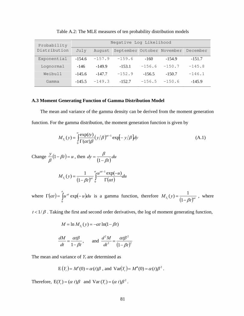
81

Table A.2: The MLE measures of ten probability distribution models

Negative Log Likelihood Probability Distribution July August September October November December

Exponential -154.6 -157.9 -159.6 -160 -154.9 -151.7

Lognormal -146 -149.9 -153.1 -156.6 -150.7 -145.8

Weibull -145.6 -147.7 -152.9 -156.5 -150.7 -146.1

Gamma -145.5 -149.3 -152.7 -156.5 -150.6 -145.9

A.3 Moment Generating Function of Gamma Distribution Model

The mean and variance of the gamma density can be derived from the moment generation

function. For the gamma distribution, the moment generation function is given by

( ) [ ]∫∞

− −Γ

=0

1 exp)(

)exp()( dyyyttyyM t

Ytββ

βαα (A.1)

Change ( ) uty=− β

β1 , then ( )du

tdy

ββ−

=1

( ) ( ) dut

uut

yMt

tYt ∫ Γ−

−=

−α α

α αβ 0

1 )exp(1

1)(

where ( ) ( )∫ −=Γa

at duuut0

expα is a gamma function, therefore ( ) tY t

yMt αβ−

=1

1)( , where

β/1<t . Taking the first and second order derivatives, the log of moment generating function,

)1ln( )(ln ttyMMtY βα −−==

t

tdt

dMββα

−=

1, and

( )22

2

2

1 tt

dtMd

ββα

−=

The mean and variance of Yt are determined as

( ) βα )()0( E tMYt =′= , and ( ) 2)()0( Var βα tMYt =′′= .

Therefore, βα ) ()E( tYt = and 2) ()(Var βα tYt = .

82

A.4 Prior Demand (Inverted Gamma Model)

The business cycle of the seasonal demand is split into two stages and stage-2 is divided

into six periods. The demand ratios of the six periods at stage-2 are taken with respect to the

demand at stage-1 collected from the past records from 1996 to 2004. [α, β] = invgamfit(D),

where D is the demand rate; The MAT LAB code is shown below:

function y = invgamfit(D)

D= 1928273; % average demand at quarter II (of 1998-2004). n = 100;

U = unifrnd(0,1,n,1); G = zeros(n,1); for i =1: n if U(i)<=0.165 G(i)= 1.67* D; elseif U(i)>0.165 & U(i)<=0.33 G(i)= 2.4*D; elseif U(i)>0.33 & U(i)<=0.50 G(i)= 2.83*D; elseif U(i)>0.50 & U(i)<=0.67 G(i)= 2.84*D; elseif U(i)>0.67 & U(i)<=0.84 G(i)= 1.65*D; else G(i)= 1.24*D; % India_supply at 2005 end end GInv = 1./G; y = gamfit(GInv); Posterior demand forecast (MATLAB-Code)

Demand forecasting from actual data [forecast for 2005] clear; % clear the memory

mu_D = 1928273.15; cov = 0.16; % COV for demand rate [COV: 0.21, 0.17, 0.24, 0.27, 0.26, 0.29] % COV for demand rate [COV: 0.16, 0.13, 0.14, 0.25, 0.19, 0.21,

% Average COV: 0.28]

% Month of July 2005 [Revised woolen apparel] t = [ 7-6]; D = [(11664953.6-9298179.8)]; % Month of August 2005 [Revised woolen apparel] %t = [ 8-7 ]; %D = [(14762640.4-11664953.6)];

83

% Month of September 2005 [Revised woolen apparel] %t = [ 9-8 ]; %D = [(19586403.9-14762640.4)];

% Month of October 2005 [Revised woolen apparel] %t = [10-9]; %D = [(25122553.0-19586403.9)];

% Month of November 2005 [Revised woolen apparel] %t = [11-10]; %D = [(28486960.3-25122553.0)];

% Month of December 2005 [Revised woolen apparel] %t = [12-11]; %D=[(30776936.0-28486960.3)];

K = length(t); % total number of inspections % Inv_COV = [1.; 1.; 1.]; % COV for each observation

% define the grid for the normal density of the measurement error: % fit a continuous inverted gamma density prior n = 10000; par = invgamfit(mu_D); a = par(1); % Shape parameter b = 1/par(2); % Scale parameter

% Define the grid over which the densities are calculated: GridLenth = mu_D/100; x = GridLenth:GridLenth:8*mu_D; N = length(x);

% the inverted gamma distributed prior is given by: Prior = exp(a*log(b)-gammaln(a)+(-a-1)*log(x)-b./x);

% inverted gamma posterior for 1 perfect inspection:555 A = a + t(K)/cov^2; % Posterior shape parameter B = b + D(K)/cov^2; % Posterior scale parameter Posterior = exp(A*log(B)-gammaln(A)+(-A-1)*log(x)-B./x);

Figure plot(x,Prior,'g--',x,Posterior,'r', 'LineWidth',2.5);

%(for Fixed COV, Sub-model B-P) plot(x,Prior,'r:',x,Posterior,'g', 'LineWidth',2.5);

%(for variable COV, Sub-model BP-I) grid legend('prior density','posterior'); title(['Forecast of woolen apparel, 2005']); xlabel('Periodic demand [July, 2005]'); ylabel('Density');

84

Figure A.1: Graphical presentation of prior and posterior density in (B-P) model

85

Figure A.2: Graphical presentation of prior and posterior density in (BP-I) model

86

APPENDIX B

ARIMA AND BAYESIAN ARIMA MODELS

B.1 Apparel Group Demand Data (units in millions) for ARIMA (0,1,1) (1,1,0)12 Period(s) of Differencing 1,12 Mean of Working Series 3,718.7 Standard Deviation 496,691 Number of Observations 101 Observation(s) eliminated by differencing 13 Autocorrelations Lag Correlation -1 9 8 7 6 5 4 3 2 1 0 1 2 3 4 5 6 7 8 9 1 Std Error 0 1.000 | |********************| 0 1 -0.496 | **********| . | 0.099 2 0.121 | . |** . | 0.121 3 -0.099 | . **| . | 0.122 4 -0.015 | . | . | 0.123 5 -0.050 | . *| . | 0.123 6 0.063 | . |* . | 0.123 7 -0.111 | . **| . | 0.124 8 0.153 | . |*** . | 0.125 9 -0.033 | . *| . | 0.126 10 -0.023 | . | . | 0.126 11 0.204 | . |****. | 0.126 12 -0.447 | *********| . | 0.130 13 0.382 | . |******** | 0.144 14 -0.188 | . ****| . | 0.154 15 0.097 | . |** . | 0.156 Inverse Autocorrelations Lag Correlation -1 9 8 7 6 5 4 3 2 1 0 1 2 3 4 5 6 7 8 9 1 1 0.646 | . |************* | 2 0.515 | . |********** | 3 0.436 | . |********* | 4 0.354 | . |******* | 5 0.295 | . |****** | 6 0.171 | . |***. | 7 0.117 | . |** . | 8 -0.001 | . | . | 9 -0.019 | . | . | 10 -0.043 | . *| . | 11 -0.021 | . | . | 12 0.059 | . |* . | 13 -0.076 | . **| . | 14 -0.035 | . *| . | 15 -0.021 | . | . |

87

Partial Autocorrelations Lag Correlation -1 9 8 7 6 5 4 3 2 1 0 1 2 3 4 5 6 7 8 9 1 1 -0.496 | **********| . | 2 -0.165 | .***| . | 3 -0.151 | .***| . | 4 -0.165 | .***| . | 5 -0.201 | ****| . | 6 -0.105 | . **| . | 7 -0.217 | ****| . | 8 -0.058 | . *| . | 9 0.004 | . | . | 10 -0.062 | . *| . | 11 0.261 | . |***** | 12 -0.311 | ******| . | 13 0.085 | . |** . | 14 0.022 | . | . | 15 0.044 | . |* . | Autocorrelation Check for White Noise To Chi- Pr > Lag Square DF ChiSq --------------------Autocorrelations-------------------- 6 28.86 6 <.0001 -0.496 0.121 -0.099 -0.015 -0.05 0.06 12 61.21 12 <.0001 -0.111 0.153 -0.033 -0.023 0.20 -0.45 Maximum Likelihood Estimation Standard Approx Parameter Estimate Error t Value Pr > |t| Lag MU 1226.80 7889.10 0.16 0.87 0 MA1,1 0.735 0.069 10.59 <.0001 1 AR1,1 -0.35 0.098 -3.59 0.0003 12

Constant Estimate 1657.36 Std Error Estimate 384482.40 AIC 2889.60 SBC 2897.49 Number of Residuals 101.00 Correlations of Parameter Estimates Parameter MU MA1,1 AR1,1 MU 1.000 -0.030 0.013 MA1,1 -0.030 1.000 0.086 AR1,1 0.013 0.086 1.000

88

Autocorrelation Check of Residuals To Chi- Pr > Lag Square DF ChiSq --------------------Autocorrelations-------------------- 6 6.11 4 0.191 -0.066 -0.167 -0.102 -0.125 -0.051 0.003 12 8.53 10 0.577 -0.057 0.089 -0.014 -0.031 0.057 -0.084 18 16.88 16 0.393 0.248 -0.102 -0.010 -0.032 0.003 -0.035 24 29.80 22 0.123 0.026 -0.089 -0.042 -0.199 0.108 0.199 Model for variable D Estimated Mean 1226.80 Period(s) of Differencing 1,12 Autoregressive Factors Factor 1: 1 + 0.35 B**(12) Moving Average Factors Factor 1: 1 - 0.735 B**(1)

The ARIMA Procedure (Women Apparel Demand Forecast)

OBS FORECAST STD L95 U95

115 2,743,345 384,482 1,989,132 3,496,275

116 3,652,484 397,727 2,781,752 4,340,812

117 4,921,266 410,544 4,349,932 5,959,235

118 5,265,951 422,973 5,250,699 6,908,722

119 2,690,180 435,047 2,606,103 4,311,455

120 2,702,920 446,795 1,826,754 3,578,157

89

Detail ARIMA Results (Women Apparel Demand Forecast)

OBS DEMAND FORECAST STD L95 U95 RESIDUAL

1 400,346 . . . . . 2 387,554 . . . . . 3 282,266 . . . . . 4 577,188 . . . . . 5 536,948 . . . . . 6 678,661 . . . . . 7 1,005,800 . . . . . 8 1,239,992 . . . . . 9 1,425,662 . . . . . 10 1,030,257 . . . . . 11 706,931 . . . . . 12 668,230 . . . . . 13 614,704 . . . . . 14 403,570 603,139 509,645 395,748 1,602,025 199,569 15 657,449 394,754 447,858 483,032 1,272,540 262,695 16 700,022 791,246 427,933 47,488 1,629,980 91,224 17 656,937 722,760 419,317 99,086 1,544,606 65,823 18 1,081,391 846,283 415,142 32,620 1,659,946 235,108 19 1,466,913 1,240,650 413,008 431,168 2,050,131 226,263 20 1,829,723 1,537,901 411,889 730,614 2,345,188 291,822 21 2,306,741 1,803,391 411,293 997,271 2,609,511 503,350 22 2,091,035 1,543,709 410,974 738,215 2,349,203 547,326 23 1,205,276 1,367,233 410,802 562,076 2,172,390 161,957 24 1,106,473 1,286,767 410,709 481,792 2,091,743 180,294 25 801,200 1,200,814 398,470 419,827 1,981,801 399,614 26 506,609 934,892 391,585 167,399 1,702,385 428,283 27 850,961 939,677 388,201 178,817 1,700,536 88,716 28 1,151,522 1,047,742 386,459 290,297 1,805,188 103,780 29 1,326,139 1,035,565 385,541 279,918 1,791,212 290,574 30 1,784,196 1,440,540 385,052 685,852 2,195,229 343,656 31 1,692,825 1,898,952 384,790 1,144,778 2,653,125 206,127 32 2,697,061 2,163,470 384,648 1,409,573 2,917,367 533,591 33 2,362,882 2,681,488 384,572 1,927,741 3,435,236 318,606 34 1,894,332 2,319,920 384,531 1,566,253 3,073,586 425,588 35 1,069,811 1,520,466 384,509 766,843 2,274,089 450,655 36 1,007,821 1,325,068 384,497 571,468 2,078,667 317,247 37 771,039 1,025,804 384,490 272,217 1,779,391 254,765 38 790,062 694,710 384,487 58,870 1,448,290 95,352 39 852,246 1,034,211 384,485 280,635 1,787,787 181,965 40 888,911 1,197,713 384,482 444,141 1,951,285 308,802 41 1,343,017 1,215,835 384,482 462,263 1,969,406 127,182 42 1,193,230 1,697,424 384,482 943,853 2,450,996 504,194

90

OBS DEMAND FORECAST STD L95 U95 RESIDUAL

43 1,349,451 1,641,607 384,482 888,035 2,395,179 292,156 44 2,018,771 2,345,044 384,482 1,591,472 3,098,616 326,273 45 2,166,497 2,210,846 384,482 1,457,275 2,964,418 44,349 46 1,906,160 1,820,951 384,482 1,067,379 2,574,523 85,209 47 1,440,326 999,153 384,482 245,581 1,752,724 441,173 48 1,007,062 1,042,691 384,482 289,119 1,796,262 35,629 49 844,005 774,097 384,482 20,525 1,527,668 69,908 50 572,093 703,218 384,482 50,354 1,456,790 131,125 51 971,594 831,376 384,482 77,805 1,584,948 140,218 52 1,100,097 999,435 384,482 245,863 1,753,007 100,662 53 1,111,883 1,383,757 384,482 630,185 2,137,329 271,874 54 1,603,974 1,376,983 384,482 623,412 2,130,555 226,991 55 2,070,043 1,508,058 384,482 754,486 2,261,629 561,985 56 3,108,957 2,445,350 384,482 1,691,778 3,198,921 663,607 57 2,744,466 2,601,279 384,482 1,847,707 3,354,851 143,187 58 2,535,864 2,307,430 384,482 1,553,859 3,061,002 228,434 59 1,664,043 1,777,842 384,482 1,024,270 2,531,414 113,799 60 1,349,740 1,446,412 384,482 692,840 2,199,983 96,672 61 1,232,589 1,233,546 384,482 479,974 1,987,118 957 62 1,257,118 1,065,144 384,482 311,573 1,818,716 191,974 63 1,293,980 1,398,739 384,482 645,167 2,152,310 104,759 64 1,205,326 1,468,935 384,482 715,364 2,222,507 263,609 65 1,243,011 1,567,830 384,482 814,259 2,321,402 324,819 66 1,270,732 1,750,317 384,482 996,745 2,503,889 479,585 67 2,059,496 1,982,340 384,482 1,228,769 2,735,912 77,156 68 3,207,157 2,913,624 384,482 2,160,053 3,667,196 293,533 69 3,356,925 2,808,264 384,482 2,054,692 3,561,836 548,661 70 3,475,341 2,728,408 384,482 1,974,836 3,481,980 746,933 71 2,162,664 2,198,463 384,482 1,444,891 2,952,034 35,799 72 981,247 1,834,590 384,482 1,081,018 2,588,161 853,343 73 1,499,544 1,477,082 384,482 723,510 2,230,654 22,462 74 849,768 1,405,176 384,482 651,604 2,158,748 555,408 75 1,127,911 1,423,935 384,482 670,364 2,177,507 296,024 76 1,168,875 1,334,786 384,482 581,214 2,088,358 165,911 77 1,172,453 1,321,118 384,482 567,546 2,074,690 148,665 78 1,449,888 1,474,116 384,482 720,544 2,227,687 24,228 79 2,185,608 2,144,870 384,482 1,391,299 2,898,442 40,738 80 3,017,227 3,266,807 384,482 2,513,236 4,020,379 249,580 81 3,920,854 3,171,678 384,482 2,418,106 3,925,250 749,176 82 3,359,162 3,375,309 384,482 2,621,737 4,128,880 16,147 83 2,413,125 2,214,737 384,482 1,461,165 2,968,309 198,388 84 1,560,131 1,391,818 384,482 638,246 2,145,389 168,313 85 1,382,481 1,733,313 384,482 979,741 2,486,885 350,832 86 1,325,336 1,228,973 384,482 475,401 1,982,545 96,363

91

OBS DEMAND FORECAST STD L95 U95 RESIDUAL

87 1,292,599 1,449,604 384,482 696,032 2,203,175 157,005 88 1,380,987 1,405,171 384,482 651,599 2,158,743 24,184 89 1,514,573 1,415,974 384,482 662,403 2,169,546 98,599 90 1,682,368 1,633,529 384,482 879,957 2,387,101 48,839 91 2,018,939 2,402,452 384,482 1,648,880 3,156,023 383,513 92 2,994,918 3,245,120 384,482 2,491,548 3,998,691 250,202 93 4,337,951 3,819,595 384,482 3,066,023 4,573,167 518,356 94 5,651,788 3,635,473 384,482 2,881,902 4,389,045 2,016,315 95 2,195,432 3,096,191 384,482 2,342,620 3,849,763 900,759 96 2,022,672 1,891,136 384,482 1,137,564 2,644,708 131,536 97 1,630,893 1,994,214 384,482 1,240,642 2,747,785 363,321 98 1,512,496 1,634,556 384,482 880,984 2,388,128 122,060 99 1,485,483 1,680,270 384,482 926,698 2,433,842 194,787 100 1,559,342 1,702,106 384,482 948,534 2,455,678 142,764 101 1,384,160 1,753,928 384,482 1,000,357 2,507,500 369,768 102 1,725,807 1,863,972 384,482 1,110,400 2,617,544 138,165 103 2,366,774 2,305,709 384,482 1,552,138 3,059,281 61,065 104 3,097,687 3,248,847 384,482 2,495,275 4,002,419 151,160 105 4,823,764 4,399,307 384,482 3,645,736 5,152,879 424,457 106 5,536,149 5,168,933 384,482 4,415,361 5,922,504 367,216 107 3,364,407 2,692,466 384,482 1,938,894 3,446,038 671,941 108 2,289,976 2,460,510 384,482 1,706,938 3,214,082 170,534 109 1,803,997 2,100,394 384,482 1,346,822 2,853,966 296,397 110 1,546,309 1,926,687 384,482 1,173,115 2,680,259 380,378 111 2,094,937 1,798,626 384,482 1,045,054 2,552,198 296,311 112 1,901,859 1,957,683 384,482 1,204,111 2,711,255 55,824 113 1,906,783 1,877,745 384,482 1,124,173 2,631,317 29,038 114 2,315,753 2,167,722 384,482 1,414,150 2,921,293 148,031 115 . 2,743,345 384,482 1,989,132 3,496,275 . 116 . 3,652,484 397,727 2,781,752 4,340,812 . 117 . 4,921,266 410,544 4,349,932 5,959,235 . 118 . 5,265,951 422,973 5,250,699 6,908,722 . 119 . 2,690,180 435,047 2,606,103 4,311,455 . 120 . 2,702,920 446,795 1,826,754 3,578,157 .

B.2 WinBUGS Code: Bayesian-sampling ARIMA (BS-ARIMA)

model { c ~ dnorm(0,0.001) alpha1 ~ dnorm (0,0.001) alpha2 ~ dnorm (0,0.001) alpha3 ~ dnorm (0,0.001) alpha4 ~ dnorm (0,0.001) beta ~ dnorm (1,0.1) tau ~ dchisqr(1) # priors for innovation and measurement error variances tau2 ~ dgamma(1,0.001)

92

# Data definitions for (t in 1:n) { y[t] <- (D[t]) } for (t in 1:N) { z[t] <- Dummy[t] } for (t in 1:N) {u[t] ~ dnorm(0,tau2)} for (j in 1:2) {RM[j] ~ dbeta(1,1) rm[j] <- 2*RM[j]-1} theta1 <- rm[1]-rm[2]*rm[1]; theta2 <- rm[2] # Model for (t in 26:n) { mu[t] <- c + alpha1*y[t-12] + alpha2*y[t-13] + alpha3*y[t-24] + alpha4*y[t-25] + u[t]-theta1*u[t-1] -theta2*u[t-2] + beta * z[t] y[t] ~ dnorm(mu[t], tau) y.new[t] ~ dnorm(mu[t], tau) sqresid[t] <- pow(mu[t] - y[t],2) } #ss <- sum(sqresid[2:n]) # Forecasts for t = n+1 … N for (t in n+1:N) { mu.new[t] <- c + alpha1*y.new[t-12] + alpha2*y.new[t-13] + alpha3*y.new[t- 24] + alpha4*y.new [t-25] + u[t]-theta1*u[t-1] -theta2*u[t-2] + beta*z[t]

y.new[t] ~ dnorm (mu.new[t], tau)} }

# Data list(D=c(400346, 387554, 282266, 577188, 536948, 678661, 1005800, 1239992, 1425662, 1030257, 706931, 668230, 614704, 403570, 657449, 700022, 656937, 1081391, 1466913, 1829723, 2306741, 2091035, 1205276, 1106473, 801200, 506609, 850961, 1151522, 1326139, 1784196, 1692825, 2697061, 2362882, 1894332, 1069811, 1007821, 771039, 790062, 852246, 888911, 1343017, 1193230, 1349451, 2018771, 2166497, 1906160, 1440326, 1007062, 844005, 572093, 971594, 1100097, 1111883, 1603974, 2070043, 3108957, 2744466, 2535864, 1664043, 1349740, 1232589,1257118, 1293980, 1205326, 1243011, 1270732, 2059496, 3207157, 3356925, 3475341, 2162664, 981247, 1499544, 849768, 1127911, 1168875, 1172453, 1449888, 2185608, 3017227, 3920854, 3359162, 2413125, 1560131, 1382481, 1325336, 1292599, 1380987, 1514573, 1682368, 2018939, 2994918, 4337951, 5651788, 2195432, 2022672, 1630893, 1512496, 1485483, 1559342, 1384160, 1725807, 1549696, 1549696, 1549696, 1549696, 1549696, 1549696, 1803997, 1546309, 2094937, 1901859, 1906783, 2315753), # Dummy Data Dummy=c(0,0,0,0,0,0,0,0,0,0,0,0, 0,0,0,0,0,0,0,0,0,0,0,0, 0,0,0,0,0,0,0,0,0,0,0,0, 0,0,0,0,0,0,0,0,0,0,0,0, 0,0,0,0,0,0,0,0,0,0,0,0, 0,0,0,0,0,0,0,0,0,0,0,0, 0,0,0,0,0,0,0,0,0,0,0,0, 0,0,0,0,0,0,0,0,0,0,0,0, 0,0,0,0,0,0, 0.39, 0.59, 0.63, 0.27, 36, 0.11, 0,0,0,0,0,0,0,0,0,0,0,0), n= 114, N=120)

93

B.3 Parameter Estimates and Demand Forecast of the BS-ARIMA Model

Table B.1: Parameter estimate of Bayesian ARIMA model (units in million)

node mean St.dev 2.50% median 97.50%

alpha1 0.15 0.16 -0.17 0.15 0.48

alpha2 0.23 0.15 -0.073 0.23 0.53

alpha3 0.68 0.19 0.29 0.68 1.05

alpha4 0.03 0.22 -0.39 0.03 0.44

theta1 -0.01 0.67 -1.45 -0.008 1.38

beta 1.00 3.22 -5.49 1.05 7.30

Table B.2: Mean, standard errors, and 95% CI using BS-ARIMA model

Node mean sd 2.50% median 97.50%

26 481,800 588,700 678,600 482,600 1,618,000 27 400,200 585,400 744,900 398,800 1,544,000 28 654,900 588,500 493,900 659,000 1,817,000 29 660,600 587,700 495,600 665,900 1,821,000 30 793,900 586,300 353,800 792,500 1,943,000 31 1,182,000 591,500 14,010 1,190,000 2,341,000 32 1,496,000 597,800 345,700 1,489,000 2,670,000 33 1,800,000 593,800 636,700 1,800,000 2,988,000 34 1,605,000 608,000 396,700 1,606,000 2,779,000 35 1,181,000 606,200 3,500 1,179,000 2,367,000 36 931,800 594,000 224,100 930,800 2,103,000 37 828,500 591,100 349,800 829,100 1,980,000 38 554,500 583,500 577,800 557,600 1,698,000 39 717,300 589,800 450,300 717,600 1,879,000 40 872,800 591,600 289,600 871,700 2,038,000 41 937,700 594,900 241,300 942,100 2,104,000 42 1,346,000 602,200 156,100 1,349,000 2,524,000 43 1,709,000 595,300 543,600 1,710,000 2,873,000 44 2,105,000 605,500 902,200 2,107,000 3,284,000 45 2,609,000 608,700 1,398,000 2,612,000 3,786,000 46 2,337,000 596,200 1,163,000 2,336,000 3,520,000 47 1,507,000 605,600 303,100 1,513,000 2,709,000 48 1,202,000 587,700 35,370 1,207,000 2,375,000 49 933,300 590,800 232,400 934,500 2,082,000 50 682,700 584,000 456,100 683,300 1,846,000 51 912,100 592,800 236,200 912,000 2,082,000 52 1,140,000 589,400 18,430 1,140,000 2,291,000 53 1,352,000 594,700 185,800 1,350,000 2,515,000 54 1,748,000 599,900 563,900 1,757,000 2,926,000 55 1,703,000 604,700 509,200 1,700,000 2,916,000 56 2,510,000 621,500 1,290,000 2,514,000 3,737,000 57 2,510,000 610,000 1,324,000 2,512,000 3,713,000

94

Node mean sd 2.50% median 97.50%

58 2,158,000 598,400 978,900 2,162,000 3,330,000 59 1,467,000 596,000 292,300 1,462,000 2,620,000 60 1,216,000 590,500 67,050 1,209,000 2,382,000 61 914,400 587,500 251,400 913,200 2,059,000 62 841,000 594,300 333,300 829,200 2,027,000 63 881,100 585,700 270,800 872,300 2,014,000 64 1,031,000 590,200 137,100 1,031,000 2,199,000 65 1,364,000 601,200 185,700 1,373,000 2,535,000 66 1,369,000 597,000 181,900 1,375,000 2,550,000 67 1,642,000 589,500 504,700 1,640,000 2,799,000 68 2,379,000 619,800 1,153,000 2,375,000 3,583,000 69 2,678,000 609,400 1,499,000 2,667,000 3,902,000 70 2,393,000 584,600 1,258,000 2,391,000 3,551,000 71 1,892,000 592,300 727,200 1,890,000 3,048,000 72 1,335,000 591,900 168,700 1,338,000 2,486,000 73 1,109,000 582,200 28,720 1,117,000 2,261,000 74 905,600 595,600 262,800 905,400 2,061,000 75 1,179,000 594,300 27,290 1,172,000 2,353,000 76 1,267,000 589,300 114,100 1,265,000 2,412,000 77 1,267,000 588,500 99,170 1,261,000 2,437,000 78 1,613,000 596,600 422,700 1,612,000 2,786,000 79 2,075,000 601,000 874,400 2,081,000 3,274,000 80 3,145,000 603,300 1,952,000 3,138,000 4,334,000 81 3,240,000 605,700 2,054,000 3,238,000 4,428,000 82 3,139,000 600,500 1,968,000 3,141,000 4,332,000 83 2,358,000 604,800 1,172,000 2,362,000 3,532,000 84 1,632,000 605,800 437,600 1,626,000 2,826,000 85 1,342,000 593,400 188,200 1,344,000 2,487,000 86 1,379,000 595,500 213,500 1,378,000 2,559,000 87 1,289,000 588,300 147,600 1,287,000 2,441,000 88 1,304,000 590,100 136,400 1,302,000 2,473,000 89 1,347,000 590,800 176,900 1,346,000 2,485,000 90 1,402,000 595,100 231,100 1,398,000 2,559,000 91 2,124,000 598,600 957,900 2,125,000 3,303,000 92 3,218,000 619,600 1,995,000 3,218,000 4,424,000 93 3,694,000 600,900 2,514,000 3,694,000 4,898,000 94 3,901,000 613,200 2,706,000 3,904,000 5,129,000 95 2,738,000 628,300 1,512,000 2,740,000 3,974,000 96 1,548,000 613,500 335,000 1,544,000 2,756,000

97 1,625,000 596,500 445,800 1,631,000 2,774,000 98 1,157,000 590,400 13,950 1,154,000 2,309,000 99 1,312,000 592,200 178,200 1,313,000 2,464,000 100 1,355,000 590,700 210,600 1,355,000 2,532,000 101 1,390,000 591,000 232,900 1,391,000 2,541,000 102 1,624,000 588,700 473,400 1,626,000 2,773,000 103 2,226,000 591,900 1,075,000 2,220,000 3,388,000 104 3,067,000 615,600 1,870,000 3,071,000 4,266,000 105 4,121,000 615,300 2,903,000 4,120,000 5,302,000 106 4,313,000 670,800 2,986,000 4,317,000 5,624,000

95

Node mean sd 2.50% median 97.50%

107 3,399,000 704,600 2,054,000 3,395,000 4,798,000 108 1,968,000 607,100 781,900 1,967,000 3,152,000 109 1,720,000 587,800 553,600 1,725,000 2,877,000 110 1,568,000 589,300 409,900 1,568,000 2,733,000 111 1,507,000 590,400 345,600 1,501,000 2,674,000 112 1,564,000 579,800 416,300 1,565,000 2,705,000 113 1,653,000 594,300 484,600 1,654,000 2,834,000 114 1,775,000 591,300 629,000 1,774,000 2,941,000 115 2,232,000 798,000 712,400 2,214,000 3,822,000 116 3,270,000 848,500 1,631,000 3,255,000 4,975,000 117 3,951,000 839,000 2,276,000 3,950,000 5,612,000

118 4,467,000 820,700 2,885,000 4,464,000 6,109,000

119 3,466,000 875,100 1,700,000 3,489,000 5,152,000

120 2,322,000 846,900 643,800 2,328,000 3,985,000

B.4 Initial Parametric Values of Multiplicative Exponential Smoothing (M-ES) Model

As a rule of thumb, a minimum of two full seasons (or 2L periods) of historical data is

needed to initialize a set of seasonal factors. Suppose data from m seasons are available and let

jx , j = 1, 2, · · ·, mL denote the average of the observations during the jth season.

(i) Estimation of trend component: The initial estimate of the trend component 0G is given by

Lmyy

G m

)1(1

0 −−

= (B.1)

(ii) Estimation of Index level: The initial estimate the index level 0R (which represents the

average level of time series at time 0) is given by

010 )2/( GLyR −= (B.2)

(iii) Estimation of seasonal components: Seasonal factors are computed for each time period t =

1, 2, · · ·, mL as the ratio of actual observation to the average seasonally adjusted value for that

season, further adjusted by the trend, that is,

0 ]2/)1[( GjLyyS

i

tt −+−= (B.3)

96

where ix is the average for the season corresponding to the t index, and j is the position of the

period t within the season. The above equation will produce m estimates of the seasonal factor

for each period.

∑−

=+=

1

0 1 m

kkLtt S

mS t = 1, 2, …, L (B.4)

)0(1∑ =

= L

t ttt

SLSS t = 1, 2, …, L (B.5)

B.5 Numerical Illustration (M-ES) Model

In Equation (B.1), the initial estimate of the trend, ])1/[()( 10 LmyyG m −−= , where my is

the average of the observations in year m, measures the average level of the time series. Similarly,

1y measures the average level of the time series for year 1. Thus ( 1yym − ) measures the

difference in these average levels. The total number of seasons between year 1 and the year m is

(m-1)L. The initial estimate of 0G is the change in average level per season from year 1 to the

year m. In this model, the proposed apparel data series (in Table A.1, Appendix A) consists of

three year of monthly data (from 2002 to 2004) to forecast demand in year 2005, then m = 3 and

L = 12. The average sales for year 1 is 1y = 2,316,670, while the average sales for year 3 is 3y =

2,740,505. Thus the initial estimate of the trend component is given by

0G = (2,740,505 - 2,316,670) / [(3-1)12] = 17,660

The number of seasons that have elapsed from the start of year 1 to the middle of year is L/2.

Following Equation (B.2), the initial estimate of index level 0R is therefore,

010 )2/( GLyR −= = 2,316,670 – (12/2) (17,660) = 2,210,711.

97

The initial estimate of seasonal factors is obtained following Equation (B.3). The calculation

of St value for the first June (6th month) for three-year sale history is illustrated as follows. The

seasonal factor for June (6th month) for the year 1 (i.e., 2003) is given by

01

66 ]2/)1[( GjLy

yS

−+−=

0.73)17,660](62/)112[(2,316,670

1,682,368=

−+−=

where demand at June 2003, y5 is 1,682,368, which the average demand of year 2003, 1y is

2,316,670; L = 12, and initial estimate of trend, 0G is 17,660. Similarly, the seasonal factor of

the month of June for the year 2 (i.e., 2004) is given by

02

1818 ]62/)1[( GLy

yS

−+−=

0.68)17,660](182/)112[(2,564,745

1,725,807=

−+−= .

The seasonal factor of June for the year 3 (i.e., 2005) is given by

03

3030 ]62/)1[( GLy

yS

−+−=

0.85)17,660](182/)112[(2,740,505

2,315,753=

−+−= .

The average seasonal index for each different season, tS (0) is given by Equation (B.5).

After obtaining the initial seasonal factor, the seasonal indices for the next years are adapted by

Ltt

tt S

Ry

S −−+= )1( γγ (B.6)

where 0 < γ < 1 is the third smoothing constant. Using Equation (B.6), the initial average

seasonal index for different seasons is illustrated in Table B.3.

98

Table B.3: Initial average seasonal index for different season

Month S1 S2 S3 tS L /∑ =

L

t tS1

tS (0) 1 0.62 0.66 0.68 0.66 1.007 0.660 2 0.59 0.61 0.58 0.59 1.007 0.598 3 0.57 0.59 0.78 0.65 1.007 0.654 4 0.61 0.62 0.71 0.64 1.007 0.649 5 0.66 0.55 0.70 0.64 1.007 0.641 6 0.73 0.68 0.85 0.75 1.007 0.756 7 0.87 0.92 1.03 0.94 1.007 0.946 8 1.28 1.20 1.20 1.23 1.007 1.234 9 1.84 1.85 1.47 1.72 1.007 1.732 10 2.38 2.11 1.89 2.13 1.007 2.142 11 0.92 1.27 1.23 1.14 1.007 1.147 12 0.84 0.86 0.80 0.83 1.007 0.840 Total = 11.91

Since 0G = 17,660, 0R = 2,210,711, S1 (0) = 0.66, then )0(] [)0(ˆ 1001 SGRy += = [2,210,711

+ 17,660] [0.11] = 1,471,073. Updating equations for level, trend, and seasonal factors are

( )00111 )1()]0(/[( GRSyR +−+= αα

= 0.2[1,382,481 / 0.66] + 0.8 [17,660 + 2,210,711] = 2,201,532

( ) 0011 )1( GRRG ββ −+−=

= 0.1[2,059,193 - 2,210,711] + 0.9 [17,660] = 742

0111 )1()/( SRyS γγ −+=

= 0.05[1,382,481 / 2,059,193] + 0.95 [0.66] = 0.66

The estimate for period 2 (February, 2002) is

[ ] )0( )1(ˆ 2112 SGRy += = [2,059,193 + 741.97] 0.59 = 1,326,191.

Therefore, y2 = 1,325,336, and the forecast error of [y2 – )0(ˆ2y ] = 1,325,336 – 1,326,191 = - 855.

The updated demand estimates and actual demand for stage-2 at year 2005 obtained by using 30

observations are shown in Table B.4.

99

Table B.4: Forecast results by M-ES model

Seasonal Factor Level Trend Forecast Actual Error RSE

Year Month

St Rt Gt ty yt E= ty - yt(E/

yt)100 2,210,711 17,660

Jan 0.660 2,201,532 14,976 1,471,073 1,382,481 88,592 -6.41

Feb 0.598 2,216,222 14,947 1,326,191 1,325,336 855 -0.06

Mar 0.654 2,180,041 9,834 1,459,866 1,292,599 167,267 -12.94

Apr 0.649 2,177,770 8,624 1,420,241 1,380,987 39,254 -2.84

May 0.641 2,221,673 12,152 1,401,502 1,514,573 113,071 7.47

Jun 0.756 2,232,086 11,978 1,688,943 1,682,368 6,575 -0.39

Jul 0.946 2,221,906 9,762 2,123,789 2,018,939 104,850 -5.19

Aug 1.234 2,270,610 13,656 2,754,587 2,994,918 240,331 8.02

Sep 1.732 2,328,234 18,053 3,957,118 4,337,951 380,833 8.78

Oct 2.142 2,404,815 23,906 5,025,037 5,651,788 626,751 11.09

Nov 1.147 2,325,849 13,619 2,785,308 2,195,432 589,876 -26.87

2003

Dec 0.840 2,353,162 14,988 1,965,159 2,022,672 57,513 2.84

Jan 0.659 2,389,821 17,155 1,585,105 1,630,893 45,788 2.81

Feb 0.598 2,431,171 19,575 1,466,303 1,512,496 46,192 3.05

Mar 0.651 2,416,800 16,180 1,584,445 1,485,483 98,962 -6.66

Apr 0.648 2,427,791 15,661 1,582,936 1,559,342 23,594 -1.51

May 0.643 2,385,262 9,842 1,540,163 1,384,160 156,004 -11.27

Jun 0.756 2,372,671 7,599 1,799,386 1,725,807 73,579 -4.26

Jul 0.945 2,405,377 10,110 2,281,466 2,366,774 85,308 3.60

Aug 1.239 2,432,601 11,821 3,027,542 3,097,687 70,145 2.26

Sep 1.739 2,510,351 18,414 4,397,216 4,823,764 426,547 8.84

Oct 2.152 2,537,494 19,287 5,502,506 5,536,149 33,643 0.61

Nov 1.137 2,637,398 27,349 3,028,953 3,364,407 335,454 9.97

2004

Dec 0.841 2,676,394 28,513 2,274,773 2,289,976 15,203 0.66

Jan 0.660 2,710,806 29,103 1,807,630 1,803,997 3,633 -0.20

Feb 0.599 2,707,794 25,892 1,638,844 1,546,309 92,535 -5.98

Mar 0.649 2,832,133 35,736 1,862,414 2,094,937 232,523 11.10

Apr 0.648 2,881,697 37,119 1,890,081 1,901,859 11,778 0.62

May 0.640 2,931,007 38,338 1,900,110 1,906,783 6,673 0.35

Stage-1 2005

Jun 0.755 2,989,304 40,334 2,285,950 2,315,753 29,803 1.29

Jul 0.95 3,022,677 39,638 2,898,443 2,834,571 63,871 -2.25

Aug 1.24 2,986,503 32,057 3,743,902 3,328,028 415,873 -12.50

Sep 1.75 2,884,235 18,624 5,074,236 4,102,475 971,761 -23.69

Oct 2.15 2,815,444 9,883 6,084,632 5,310,310 774,322 -14.58

Nov 1.14 2,865,449 13,895 3,292,890 3,460,540 167,650 4.84

Stage-2 2005

Dec 0.84 2,845,346 10,495 2,403,797 2,280,498 123,299 -5.41

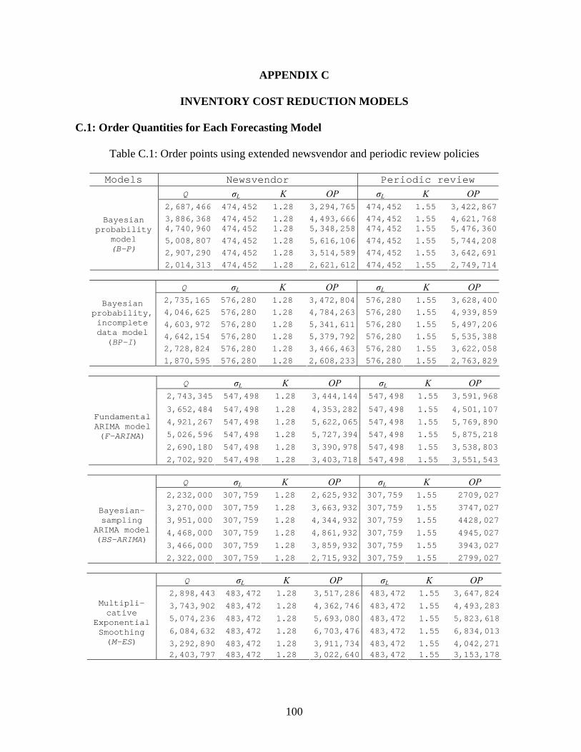
100

APPENDIX C

INVENTORY COST REDUCTION MODELS

C.1: Order Quantities for Each Forecasting Model

Table C.1: Order points using extended newsvendor and periodic review policies

Models Newsvendor Periodic review Q σL K OP σL K OP

2,687,466 474,452 1.28 3,294,765 474,452 1.55 3,422,8673,886,368 474,452 1.28 4,493,666 474,452 1.55 4,621,7684,740,960 474,452 1.28 5,348,258 474,452 1.55 5,476,3605,008,807 474,452 1.28 5,616,106 474,452 1.55 5,744,2082,907,290 474,452 1.28 3,514,589 474,452 1.55 3,642,691

Bayesian probability

model (B-P)

2,014,313 474,452 1.28 2,621,612 474,452 1.55 2,749,714

Q σL K OP σL K OP 2,735,165 576,280 1.28 3,472,804 576,280 1.55 3,628,4004,046,625 576,280 1.28 4,784,263 576,280 1.55 4,939,8594,603,972 576,280 1.28 5,341,611 576,280 1.55 5,497,2064,642,154 576,280 1.28 5,379,792 576,280 1.55 5,535,3882,728,824 576,280 1.28 3,466,463 576,280 1.55 3,622,058

Bayesian probability, incomplete data model

(BP-I)

1,870,595 576,280 1.28 2,608,233 576,280 1.55 2,763,829

Q σL K OP σL K OP 2,743,345 547,498 1.28 3,444,144 547,498 1.55 3,591,968

3,652,484 547,498 1.28 4,353,282 547,498 1.55 4,501,107

4,921,267 547,498 1.28 5,622,065 547,498 1.55 5,769,890

5,026,596 547,498 1.28 5,727,394 547,498 1.55 5,875,218

2,690,180 547,498 1.28 3,390,978 547,498 1.55 3,538,803

Fundamental ARIMA model (F-ARIMA)

2,702,920 547,498 1.28 3,403,718 547,498 1.55 3,551,543

Q σL K OP σL K OP 2,232,000 307,759 1.28 2,625,932 307,759 1.55 2709,027

3,270,000 307,759 1.28 3,663,932 307,759 1.55 3747,027

3,951,000 307,759 1.28 4,344,932 307,759 1.55 4428,027

4,468,000 307,759 1.28 4,861,932 307,759 1.55 4945,027

3,466,000 307,759 1.28 3,859,932 307,759 1.55 3943,027

Bayesian-sampling

ARIMA model (BS-ARIMA)

2,322,000 307,759 1.28 2,715,932 307,759 1.55 2799,027

Q σL K OP σL K OP 2,898,443 483,472 1.28 3,517,286 483,472 1.55 3,647,824

3,743,902 483,472 1.28 4,362,746 483,472 1.55 4,493,283

5,074,236 483,472 1.28 5,693,080 483,472 1.55 5,823,618

6,084,632 483,472 1.28 6,703,476 483,472 1.55 6,834,013

3,292,890 483,472 1.28 3,911,734 483,472 1.55 4,042,271

Multipli-cative

Exponential Smoothing (M-ES)

2,403,797 483,472 1.28 3,022,640 483,472 1.55 3,153,178

101

C.2 Numerical Illustration of Inventory Cost (units in million)

Step 1: One choice, just satisfy order point, Q1.

Step 2: Two choices, either j1* = 1 or j2* = 2.

Step3: Two choices, j3* = 2, 3.

Step 4: Two choices, j4* = 3, 4.

2

37.180

37.180 014.0)34.4(2591.71 06.183)34.4(624.)34.488.2(25015.0

min

2by procure ,1by procure ,

min

*2

222*

1

21111*2

=

=

⎩⎨⎧

=++=+++

=

⎩⎨⎧

++++

=

j

QCAFQhQCA

F

3

93.307

93.307 54.127016.037.180 54.316 32.331.241014.009.719

55.32232.302.620.313015.0min

3by procure ,)(2by procure ,)( 1by procure ,))()(

min

*3

333*

2

323222*

1

3232132111*

3

=

=

⎪⎩

⎪⎨

⎧

=++=+++

=+++=

⎪⎩

⎪⎨

⎧

++++++

++++++=

j

QCAFQhQQCAF

QhQQhQQQCAF

3

66.442

73.444 78.136016.093.307

66.442 41.386.258016.037.180min

4by procure ,QC

3by procure ,)(min

*4

444*

3

434333*

2*4

=

=

⎪⎩

⎪⎨⎧

=++

=+++=

⎪⎩

⎪⎨⎧

++

++++=

j

AF

QhQQCAFF

1

91.71)87.2(25015.0

*2

111*

1

=

=+=+=

j

QCAF

102

Step 5: Three choices, j5* = 3, 4, 5.

Step 6: Four choices, j6* = 3, 4, 5, 6.

And so on.

C.3 Optimal Inventory Cost Using Newsvendor Policy (units in million)

Table C.2: Inventory cost based on (B-P) Model (units in million)

Cost of ordering at stage-2, 2005 Fj Jul Aug Sep Oct Nov Dec

1 71.91* 183.06 322.55 469.58 563.59 633.822 180.37* 316.54 460.16 552.03 620.703 307.93* 442.66* 528.98* 593.59*4 444.73 532.34 597.895 531.57 598.066 603.92

Min 71.91 180.37 307.93 442.66 528.98 593.59j*(k) 1 2 3 3 3 4

3

98.528

56.581 89.88017.065.442

34.532 13.226.222016.093.307

98.528 13.246.5591.340016.037.180

min

,QC

4by procure ,)(

3by procure ,)()(

min

*5

555*

4

545444*

3

5454354333*

2

*5

=

=

⎪⎪⎩

⎪⎪⎨

⎧

=++

=+++

=++++

=

⎪⎪⎩

⎪⎪⎨

⎧

++

++++

+++++++

=

j

AF

QhQQCAF

QhQQhQQQCAF

F

103

Table C.3: Inventory cost based on forecasts for (BP-I) Model (units in million)

Cost of ordering at stage-2, 2005 Fj

Jul Aug Sep Oct Nov Dec

1 86.84* 209.43 349.63 494.20 589.51 662.862 206.46* 343.33 484.54 577.69 649.403 334.67* 467.14* 554.66* 622.14*4 469.18 558.01 626.475 557.29 626.736 632.93

Min 86.84 206.46 334.67 467.14 554.66 622.14j*(k) 1 2 3 3 3 3

Table C.4: Inventory cost based on (F-ARIMA) Model (units in million)

Cost of ordering at stage-2, 2005 Fj Jul Aug Sep Oct Nov Dec

1 86.12* 197.67 345.24 499.14 592.38 688.092 194.96* 339.02 489.36 580.48 674.073 329.91* 470.94* 556.56* 644.62*4 473.11 560.00 649.345 559.12 649.746 658.69

Min 86.12 194.96 329.91 470.94 556.56 644.62

j*(k) 1 2 3 3 3 3

Table C.5: Inventory cost based on (BS-ARIMA) Model (units in million)

Cost of ordering at stage-2, 2005 Fj

Jul Aug Sep Oct Nov Dec

1 65.66* 159.55 273.59 404.24 510.38 586.752 157.28* 268.61 396.23 499.95 574.633 261.57* 381.29* 478.75* 549.01*4 383.13 482.04 553.335 481.67 553.976 560.24

Min 65.66 157.28 261.57 381.29 478.75 549.01j*(k) 1 2 3 3 3 3

104

Table C.6: Inventory cost based on (M-ES) Model (units in million)

Cost of ordering at stage-2, 2005 Fj

Jul Aug Sep Oct Nov Dec

1 87.95* 199.74 349.17 529.31 636.86 721.862 197.03* 342.91 518.86 623.98 707.093 333.68* 498.75* 597.51* 675.71*4 501.28 601.52 680.865 600.47 680.946 688.21

Min 87.95 197.03 333.68 498.75 597.51 675.71j*(k) 1 2 3 3 3 3

C.4: Optimal Inventory Cost Using Periodic Review Policy (units in million)

Table C.7: Inventory cost based on (B-P) Model (units in million)

Cost of ordering at stage-2, 2005 Fj Jul Aug Sep Oct Nov Dec

1 85.59* 204.01 347.76 502.12 602.28 679.602 201.14* 341.47 492.25 590.13 665.743 332.59* 474.04* 566.01* 637.15*4 476.21 569.56 641.735 568.77 641.976 648.52

Min 85.59 201.14 332.59 474.04 566.01 637.15

j*(k) 1 2 3 3 3 3

Table C.8: Inventory cost based on (BP-I) Model (units in million)

Cost of ordering at stage-2, 2005 Fj Jul Aug Sep Oct Nov Dec

1 90.72* 217.30 361.59 510.34 609.93 687.652 214.24* 355.10 500.39 597.72 673.713 346.18* 482.49* 573.94* 645.44*4 484.59 577.40 649.945 576.68 650.266 656.87

Min 90.72 214.24 346.18 482.49 573.94 645.44

j*(k) 1 2 3 3 3 3

105

Table C.9: Inventory cost based on (F-ARIMA) Model (units in million)

Cost of ordering at stage-2, 2005 Fj Jul Aug Sep Oct Nov Dec

1 89.81* 205.15 356.60 514.48 611.78 711.652 202.36* 350.20 504.42 599.51 697.163 340.85* 485.52* 574.87* 666.75*4 487.75 578.42 671.645 577.55 672.106 681.43

Min 89.81 202.36 340.85 485.52 574.87 666.75

j*(k) 1 2 3 3 3 3

Table C.10: Inventory cost based on (BS-ARIMA) Model (units in million)

Cost of ordering at stage-2, 2005 Fj Jul Aug Sep Oct Nov Dec

1 82.00* 195.28 343.91 513.85 646.85 741.742 192.54* 337.63 503.62 633.61 726.393 328.45* 484.18* 606.30* 693.60*4 486.57 610.52 699.085 609.96 699.796 707.55

Min 82.00 192.54 328.45 484.18 606.30 693.60

j*(k) 1 2 3 3 3 3

Table C.11: Inventory cost based on (M-ES) Model (units in million)

Cost of ordering at stage-2, 2005 Fj

Jul Aug Sep Oct Nov Dec

1 91.21* 206.35 359.20 542.85 653.99 742.662 203.56* 352.78 532.16 640.78 727.483 343.34* 511.62* 613.68* 695.26*4 514.21 617.78 700.555 616.74 700.696 708.29

Min 91.21 203.56 343.34 511.62 613.68 695.26

j*(k) 1 2 3 3 3 3

106

VITA

Mohamed Anwar A. Rahman was born in Dhaka, Bangladesh. He received his Bachelor

in Mechanical Engineering and Master of Science in Industrial and Production Engineering

degrees from Bangladesh University of Engineering and Technology (BUET), Dhaka, in 1995

and 1998, respectively. He was employed in Navana Ltd. - a Toyota Automobiles Assembly

Plant, from 1997 to 1998. Then, he joined the graduate program in the Department of Industrial

Engineering at Louisiana State University, Baton Rouge, Louisiana, in the spring 2000. He

received the degree of Master of Science in Industrial Engineering from Louisiana State

University, Baton Rouge, Louisiana, in May 2003. He has published one paper in European

Journal of Operational Research. His research interests include supply chain management,

manufacturing process, scheduling, industrial simulation, applied probability, quality control,

reliability and replacement models, data analysis and interpretation, forecasting modeling, and

operations-marketing interface. He also received a Master of Science degree in applied

statistics from Louisiana State University, Baton Rouge, Louisiana, in December 2007. He is a

member of the Institute of Industrial Engineers (IIE), and the Institute for Operations Research

and Management Science (INFORMS).