Intermittent Demand Forecasting for Inventory Control: The Impact of Temporal and Cross-sectional Aggregation

by

Ngan Ngoc Chau Ph.D., Business Administration, University of Central Florida, 2012

B.S., Information Technology, Vietnam National University, 2005

B.B.A, Posts & Telecommunications Institute of Technology, 2004

SUBMITTED TO THE PROGRAM IN SUPPLY CHAIN MANAGEMENT

IN PARTIAL FULFILLMENT OF THE REQUIREMENTS FOR THE DEGREE OF

MASTER OF OF ENGINEERING IN SUPPLY CHAIN MANAGEMENT AT THE

MASSACHUSETTS INSTITUTE OF TECHNOLOGY

May 2020

© 2020 Ngan Ngoc Chau. All rights reserved. The authors hereby grant to MIT permission to reproduce and to distribute publicly paper and electronic

copies of this thesis document in whole or in part in any medium now known or hereafter created.

Signature of Author: ____________________________________________________________________ Department of Supply Chain Management

May 8, 2020

Certified by: __________________________________________________________________________ Dr. Nima Kazemi

Postdoctoral Associate Thesis Advisor

Accepted by: __________________________________________________________________________ Prof. Yossi Sheffi

Director, Center for Transportation and Logistics Elisha Gray II Professor of Engineering Systems Professor, Civil and Environmental Engineering

2

Intermittent Demand Forecasting for Inventory Control: The Impact of Temporal and Cross-sectional Aggregation

by

Ngan Ngoc Chau

Submitted to the Program in Supply Chain Management on May 8, 2020 in Partial Fulfillment of the

Requirements for the Degree of Master of Engineering in Supply Chain Management

ABSTRACT

Managing intermittent demand is a challenging operation in many industries since this type of demand is difficult to forecast. This challenge makes it hard to estimate inventory levels and thus affects service levels. The purpose of this study is to examine the impact of multiple levels of data aggregation on forecasting intermittent demand, and subsequently, on inventory control performance. In particular, we propose a procedure that integrates lead-time and customer heterogeneity into the forecasting using temporal and cross-sectional aggregation. Using data from a real-world setting and simulation, our analysis revealed that when high service levels were important for the company operations, the forecasting approach using temporal aggregation that incorporates lead-time information yielded a higher level of inventory efficiency in terms of both the holding cost and the realized service level. It appeared that when forecasts using temporal aggregation were augmented with information about customer behavior, their purchase patterns might be a helpful consideration for enhancing inventory performance. These findings allow us to provide useful recommendations for improving the current forecasting procedure and inventory control to the sponsor company of this project.

Thesis Advisor: Dr. Nima Kazemi Title: Postdoctoral Associate

3

ACKNOWLEDGMENTS

I would like to thank my thesis advisor Dr. Nima Kazemi for his encouragement and valuable comments on my work. I would also like to express my gratitude to the executives and personnel at G.L. Huyett who sponsored and were actively involved in this research project: Mr. Timothy O’Keeffe - CEO of G.L. Huyett, Ms. Sarah Sinnett – VP of Marketing and Technology, and Mr. Jacob Baker. Without their collaboration and relevant input, this project could not have been successfully conducted.

4

TABLE OF CONTENTS LIST OF FIGURES ........................................................................................................................ 5

LIST OF TABLES .......................................................................................................................... 6

1. INTRODUCTION ...................................................................................................................... 7

1.1 Research Motivation ............................................................................................................. 7

1.2 Problem Statement ................................................................................................................ 8 1.3 Research Question and Contribution ................................................................................... 10

2. LITERATURE REVIEW ......................................................................................................... 12

2.1 Intermittent Demand Time-series Forecasting Methods ..................................................... 12

2.2 Inventory Control for Intermittent Demand ........................................................................ 17

2.3 Data Aggregation ................................................................................................................ 19

2.3.1 Temporal Aggregation .................................................................................................. 19

2.3.2 Cross-sectional Aggregation ......................................................................................... 22

3. METHODOLOGY ................................................................................................................... 26 3.1 Data Collection .................................................................................................................... 27

3.2 Data Preparation .................................................................................................................. 27

3.3 Data Analysis ...................................................................................................................... 27

3.4 Demand Forecasting ............................................................................................................ 27

3.4.1 Time-series Forecasting Methods ................................................................................. 28

3.4.2 Data Aggregation .......................................................................................................... 29

3.5 Inventory Control ................................................................................................................ 31

3.6 Performance Assessment ..................................................................................................... 32

4. DATA ....................................................................................................................................... 34 4.1 Data Preparation .................................................................................................................. 34

4.2 Data Analysis ...................................................................................................................... 36

5. RESULTS ................................................................................................................................. 39

5.1 Temporal Aggregation ........................................................................................................ 39

5.2 Cross-sectional Aggregation ............................................................................................... 49

6. DISCUSSION ........................................................................................................................... 53

6.1 Result Implications .............................................................................................................. 53

6.2 Limitation and Future Research .......................................................................................... 55 7. CONCLUSION ......................................................................................................................... 56

REFERENCES ............................................................................................................................. 57

5

LIST OF FIGURES

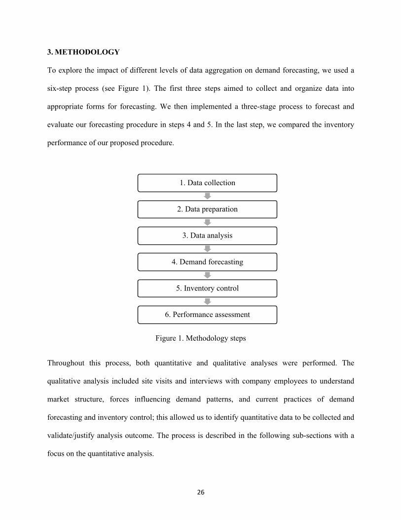
Figure 1. Methodology steps ......................................................................................................... 26

Figure 2. Cross-sectional aggregation based on customer heterogeneity ..................................... 30

Figure 3. Simulation flow chart .................................................................................................... 32

Figure 4. Lead-time distribution ................................................................................................... 37

Figure 5. Efficiency curves for weekly and monthly time buckets .............................................. 44

Figure 6. Efficiency curves for weekly and monthly time buckets with a warm-up period ......... 45

Figure 7. Efficiency curves for the baseline and temporal aggregation ....................................... 47

Figure 8. Efficiency curves for forecasting methods .................................................................... 48

Figure 9. An illustration of customer purchase patterns of an SKU ............................................. 51

6

LIST OF TABLES

Table 1. Descriptive statistics of monthly demand ....................................................................... 36

Table 2. Descriptive statistics of weekly demand ......................................................................... 37

Table 3. Descriptive statistics of lead-time and unit cost ............................................................. 37

Table 4. SKU demand classification ............................................................................................. 38

Table 5. Inventory performance of the baseline ........................................................................... 40

Table 6. Inventory performance of temporal aggregation ............................................................ 41

Table 7. Inventory performance of the baseline with a warm-up period ...................................... 42

Table 8. Inventory performance of temporal aggregation with a warm-up period ....................... 43

Table 9. The inventory performance of forecasting on regular customer demand ....................... 52

7

1. INTRODUCTION

1.1 Research Motivation

Products with intermittent demand − such as engineering spares and spare parts kept at the

wholesaling/retailing level − are found in many industrial settings including automotive,

aerospace, IT, and the military and may collectively account for up to 60 percent of the total

inventory value (Johnston, Boylan, & Shale, 2003). Intermittent demand occurs when a product

experiences several periods of zero demand interspersed by occasional non-zero demands.

Managing such items is a challenging operation since their demand nature makes it difficult to

forecast, and subsequently, to estimate inventory levels. As a result, organizations facing such

demand often experience both high inventory levels and unsatisfactory service levels at the same

time.

Research on intermittent demand has emerged as a separate research stream since the proposed

method of Croston in 1972 (Croston, 1972). Further, the growing business value generated by

intermittent demand items such as service parts has drawn substantial attention from researchers

(e.g., Hu, Boylan, Chen, & Labib, 2018). For example, according to a study by McKinsey &

Company, the global value for automotive service parts business was approximately $760 billion

in 2015 and expected to increase to $1,196 billion in 2030 (Breitschwerdt, Cornet, Kempf,

Michor, & Schmidt, 2017). Because of their practical and economic importance, several methods

and techniques for forecasting and inventory control of intermittent demand items have been

incorporated into various enterprise software packages. Nevertheless, there is a lack of recently

developed methods in commercial software (Hu et al., 2018). For instance, typical software

8

packages do not support temporal aggregation (defined in Section 2.3.1), although it may be

helpful for decision making (Syntetos, Babai, Boylan, Kolassa, & Nikolopoulos, 2016).

The general purpose of this study is to evaluate the impact of our proposed forecasting approach

on inventory performance. This research endeavor is validated in the context of a master

distributor of nonthreaded fasteners and specialty components located in the United States, G.L.

Huyett. The company offers more than 150,000 stock keeping units (SKUs) and many of them

(over 70 percent) exhibit intermittent demand, complicating forecasting and subsequently setting

inventory levels. Further, as a master distributor that sells a variety of manufactured products

through other distributors, G.L. Huyett is expected to maintain a very broad inventory as well as

high service levels.

1.2 Problem Statement

In practice, demand information for a product is captured at the individual order level at a

specific point in time. This information is then aggregated along some dimensions such as time,

customer, or location to inform decision makers at different organizational levels; for example,

inventory managers focus on lead time demand forecast per SKU while distribution managers

want weekly or monthly demand forecast per customer/location. From an academic perspective,

for a given level of aggregation required by decision-makers, it is not obvious what is the

optimal strategy of data aggregation for input and output of forecasting (Syntetos et al., 2016).

From the literature, there are two types of aggregation: temporal and cross-sectional. Temporal

aggregation refers to a process in which demand recorded in higher-frequency time buckets (e.g.,

hourly, daily) is combined in lower-frequency time buckets (e.g., weekly, monthly). Meanwhile,

9

cross-sectional aggregation is a process that combines multiple time series based on the product

family, location, or customer. Previous work has predominantly investigated these two types

separately although their combination has been identified to yield potential benefits (e.g.,

Syntetos et al., 2016).

More specifically, temporal aggregation focusing on the lead-time and cross-sectional

aggregation focusing on customer heterogeneity have been shown separately to be effective tools

for reducing demand intermittency and facilitating better inventory performance (e.g., Babai, Ali,

& Nikolopoulos, 2012; Zotteri, Kalchschmidt, & Caniato, 2005). Further, recent studies on

combining multiple ways of aggregation have confirmed an improvement in forecast

performance (Lei, Li, & Tan, 2016; Lei, Yin, Li, & Tan, 2017; Petropoulos & Kourentzes, 2015;

Spiliotis, Petropoulos, Kourentzes, & Assimakopoulos, 2020). Therefore, we believe that

focusing on lead-time and customer heterogeneity has important implications for intermittent

demand. First, temporal aggregation enables: (1) reducing the presence of zero-demand

occurrences, which leads to better extrapolation; and (2) focusing directly on lead-time demand

for inventory control instead of point estimates over the same period (Babai et al., 2012).

Second, it has been proven that understanding the demand generation process may yield

substantial benefits when demand distribution tends to be compound in nature; for example,

customer heterogeneity could significantly influence demand patterns (Kalchschmidt, Verganti,

& Zotteri, 2006). Hence, incorporating customer differences in terms of, for instance, purchase

behavior when examining lead-time demand would potentially improve the performance of the

overall system.

10

1.3 Research Question and Contribution

Our study explores the synergy of benefits from temporal and cross-sectional aggregation. In

particular, this study addresses the following question: Does integrating lead-time and customer

heterogeneity help organizations improve intermittent demand forecasting and minimize

inventory costs while maintaining a satisfactory service level?

Such a combination has not been explored in the literature; thus our study contributes to the area

of data aggregation in forecasting and inventory control. Our proposed procedure is empirically

assessed in a real-world setting. This assessment allows us to provide useful recommendations

for improving their current forecasting procedures and inventory control to industries/companies

that may have the same problem.

More specifically, our analysis of temporal aggregation highlights (1) the inventory efficiency of

this forecasting approach; (2) the distinct effect of aggregation applied to the input data and the

forecasting procedure; and (3) the heterogeneous effect of temporal aggregation on various

forecasting methods used. It appears that when forecasts using temporal aggregation are

augmented with information about customer behavior, their purchase patterns may be a helpful

consideration for enhancing inventory performance; however, this evidence is relatively weak

and exploratory in nature.

The rest of this thesis is organized as follows. Section 2 reviews the literature related to our

research. Sections 3 and 4 describe our methodology and the data used for empirical assessment,

11

respectively. We report the results of our analysis in Section 5. A discussion of the results and

the general research project is provided in Section 6. Section 7 concludes our study.

12

2. LITERATURE REVIEW

The purpose of this study is to examine to impact of data aggregation on intermittent demand

forecasting for inventory control. It follows that this section reviews three research areas that are

closely related to intermittent demand time-series forecasting methods, inventory control, and

data aggregation. First, an understanding of different forecasting methods in the context of

intermittent demand helps us identify those that may be useful to deploy in our research. Second,

since the goal of our forecasting approach is to support inventory control decisions, a review of

research on inventory control allows us to develop an appropriate framework for performance

assessment. Lastly, previous studies of data aggregation help us elaborate on the effectiveness of

different types of aggregation and incorporate them into our proposal.

2.1 Intermittent Demand Time-series Forecasting Methods

Since our study employs time-series forecasting methods, we will focus on exploring their usage

for intermittent demand. Note that a comprehensive review of forecasting methods for general

time series can be found in Syntetos et al. (2016); a discussion of other methods (e.g., causal

models) in the context of intermittent demand is beyond the scope of this study and is provided

in Hu et al. (2018) and Nikolopoulos (2020).

Intermittent demand is characterized by several periods of zero demand interspersed by

occasional non-zero demands. It follows that conventional time-series methods such as moving

average and simple exponential smoothing (SES) would over-estimate the mean demand if

applied immediately after a non-zero demand incident (Croston, 1972). To resolve this issue,

Croston (1972) separated the demand series into two components – i.e., demand sizes and inter-

13

demand intervals – and used SES for each of them; the per-period forecast was derived from the

ratio of the smoothed demand size to the inter-demand interval. Essentially, Croston (1972)

captures the compound nature of intermittent demand distribution. This method, however,

assumes a stationary mean model (i.e., without trend and seasonality; for extended models, see

Altay, Rudisill, & Litteral, 2008; Bermúdez, Segura, & Vercher, 2006).

In practice, Croston’s method is widely used in industry and is available in various forecasting

software packages (Syntetos & Boylan, 2005) although it is a biased estimator (Syntetos &

Boylan, 2001). Later works proposed different correction factors to overcome the bias associated

with Croston’s method (Levén & Segerstedt, 2004; Syntetos & Boylan, 2005; Teunter, Syntetos,

& Zied Babai, 2011; Teunter & Sani, 2009). Nevertheless, empirical studies have revealed

inconsistency on which is “the best” method (Bacchetti & Saccani, 2012).

When investigating the inconsistency of empirical work, Bacchetti and Saccani (2012) pointed

out several reasons including (1) undifferentiated application of forecasting methods on items

with heterogeneous demand patterns, and (2) inappropriate/inconsistent usage of forecast

performance metrics. We first address the former (the latter will be discussed at the end of this

sub-section) using the proposed three-phase forecasting process from Boylan and Syntetos

(2010). These authors argued that before applying any methods, it is important to define the

rules/protocols for evaluating and classifying the demand pattern (such as the level of

intermittence). The purpose of classification is to identify the appropriate forecasting method for

each demand category.

14

One of the first papers considering such a task is Williams (1984) in which demand classification

was based on partitioning the variance of the demand during the lead time; each constituent part

became a dimension for classification. Williams (1984) identified three demand categories when

lead times were constant – smooth, slow-moving, and sporadic – based on two dimensions: (1)

the mean number of lead times between demands (how often demand occurred); and (2) the

lumpiness of demand – measured via a product of the former dimension and the variability of the

non-zero demand sizes. Since then, many alternative classification schemes have emerged

(Eaves & Kingsman, 2004; Petropoulos & Kourentzes, 2015). The following describes the three

recent schemes that have been empirically validated (i.e., Kostenko & Hyndman, 2006; Lengu,

Syntetos, & Babai, 2014; Syntetos, Boylan, & Croston, 2005).

Syntetos et al. (2005) proposed a classification scheme (hereafter SBC) with two dimensions: the

average inter-demand interval (p) and the squared coefficient of variation of the demand sizes

(CV2). This outcome was derived from the comparisons of the theoretical mean square errors

(MSEs) of three forecasting methods: (1) Croston; (2) Syntetos and Boylan Approximation

(SBA) – a bias-adjusted version of Croston; and (3) SES. It has been shown that SBA was

optimal for p > 1.32 and/or CV2 > 0.49; otherwise, Croston was dominant. Accordingly, the

classification scheme consisted of four distinct demand categories – erratic, lumpy, smooth, and

intermittent – and their recommended forecasting methods – Croston for smooth demand and

SBA for the others. Kostenko and Hyndman (2006) elaborated the comparison between SBA and

Croston in Syntetos et al. (2005) and suggested another scheme (hereafter KH): using SBA for

CV2 > 2-(3/2)p and Croston otherwise. Based on this boundary, there were two demand

categories: smooth (when Croston was better) and lumpy (when SBA was better). Using a

15

sample of more than 10,000 SKUs from three different industries, Heinecke, Syntetos, and Wang

(2013) found that despite its simplicity, SBC did not perform as well as KH.

Unlike SBC and KH, which assumed the demand arrival process as a Bernoulli one (time is a

discrete variable), Lengu et al. (2014) assumed a Poisson process (time is a continuous variable)

and classified demand based on the distributional properties of the customer order sizes. Note

that the “order size” refers to the number of units in a customer order while the “demand size”

refers to the total number of units ordered during a given period of time. There were four

categories corresponding to four order size distributions: Geometric, Logarithmic series, Poisson,

and Pascal. Based on their differences, Lengu et al. (2014) developed a classification scheme

using the mode 𝑚"(𝑋) and the squared coefficient of variation of the order sizes CV2(X) as

follows:

(A) SKUs with 𝑚"(𝑋) = 1 and CV2(X) < 1 may have a Poisson-Geometric distribution;

(B) SKUs with 𝑚"(𝑋) = 1 and CV2(X) ³ 1 may have a Poisson-Logarithmic series

distribution;

(C) SKUs with 𝑚"(𝑋) ³ 2 and CV2(X) < 1 may have a Poisson-Poisson distribution; and

(D) SKUs with 𝑚"(𝑋) ³ 2 and CV2(X) ³ 1 may have a Poisson-Pascal distribution.

Despite their advantages and disadvantages, among these above schemes, SBC is widely adopted

in the literature. Hence, this study follows this scheme due to its parsimony and comparability to

previous work. In particular, we deploy three parametric forecasting methods – Croston, SBA,

and SES – in our analysis when examining different types of data aggregation. Another reason

for selecting these methods is that their effectiveness in inventory control has been proven in the

16

literature when comparing with non-parametric approaches such as bootstrapping (Syntetos, Zied

Babai, & Gardner, 2015).

Lastly, we review the usage of various forecast accuracy metrics when evaluating time-series

forecasting methods. In general, there are two basic types of metrics: scale-dependent and scale-

independent (see Hyndman & Koehler, 2006 for further refinement). The former has its scale

depending on the scale of the data; thus it is useful to compare different methods applied to the

same data set. By contrast, the latter can be used to compare forecast performance across

different data sets. Examples of the former include root mean square error (RMSE) and mean

absolute error (MAE), and of the latter include mean absolute percent error (MAPE), mean

absolute scaled error (MASE), and relative geometric root mean squared error (RGRMSE). It is

important to notice that some popular measures are ill-suited for intermittent demand because

they become infinite or undefined with zero values in the demand series; for example, the

commonly used metric MAPE cannot be deployed because of the “division by zero” problem

(more examples can be found in Hyndman, 2006). Among various measures, MASE has been

highly recommended for intermittent demand because it is scale-free and less sensitive to the

existence of trend and/or seasonality (Hyndman, 2006); RGRMSE has also been shown to be a

robust measure in the presence of outliers (Syntetos & Boylan, 2005). Another important

measure for our study is the RMSE. Despite its scale-dependency it is a useful measure to

estimate demand variation (or standard deviation) for inventory control purposes. In this study,

smoothed mean square error (MSE) has been used to estimate the variance of our forecast.

17

2.2 Inventory Control for Intermittent Demand

Forecasting is an integral part of inventory management systems (Cavalieri, Garetti, Macchi, &

Pinto, 2008). In fact, our purpose for examining forecasting methods is to support inventory-

related decisions; therefore, these methods should be evaluated based on their consequence –

a.k.a., inventory performance. In other words, inventory and service level measures should play

an important role in determining the optimal forecasting procedure (Petropoulos, Wang, &

Disney, 2019).

To obtain these measures, a simulation needs to be conducted with a defined inventory control

policy. Typically, a periodic review policy (vis-à-vis continuous review policy) is preferred for

intermittent demand items because of its relevance to practical situations, such as consolidating

orders to a common supplier and convenient delivery schedule (see Sani & Kingsman, 1997 for a

discussion of various periodic policies). For this study, we adopt the order-up-to policy (R, S) as

the inventory replenishment policy (defined in the next paragraph) due to its simple structure and

ease of implementation; where R and S represent the review period and the order-up-to-level,

respectively. This policy has been widely adopted in many studies about intermittent demand

(Babai et al., 2012; Syntetos, Babai, Dallery, & Teunter, 2009; Syntetos & Boylan, 2006;

Syntetos, Nikolopoulos, & Boylan, 2010; Syntetos et al., 2015; Teunter, Syntetos, & Babai,

2010).

The (R, S) policy is defined as follows. At the end of every review period R, the inventory

position is assessed such that if it is smaller than the order-up-to-level S, then a replenishment

order will be triggered to raise the inventory position to S. For simplicity purposes, it is assumed

18

that any unsatisfied demand is backlogged and capacity for supply is infinite. The determination

of R and S is followed by the instructions in Silver, Pyke, and Peterson (1998, p. 276); in

particular, R is assumed to be fixed when deriving the value of S. In practice, the value of R tends

to be predetermined by external factors such delivery schedules (though it can be selected via

cost optimization). The value of S needs to cover the demand during the review time R and the

lead time of a purchase delivery L with a target service level α. Given a continuous demand

distribution during the time horizon (R+L), the order-up-to-level S is determined by Equation (1)

S = H-1(α) (1)

where H-1 is the inverse cumulative distribution function of the demand during (R+L) period

with the mean and standard deviation estimated by the forecast demand during (R+L) and the

standard deviation of errors of forecasts over (R+L).

The performance of the above policy can be evaluated via financial, operational, and service-

related metrics (Petropoulos et al., 2019). Financial metrics consider costs incurred in the system

such as inventory holding, backlogs, and ordering. Operational metrics include order and

inventory variance. Lastly, service-related metrics consist of cycle service level (i.e., the

percentage of periods that end with non-negative inventory) and fill rate (i.e., the proportion of

the demand satisfied directly from the stock). It is known in the literature that there are trade-offs

between these metrics and previous work has adopted multiple criteria for evaluation purposes

such as a trade-off curve between the holding cost and service level (Babai et al., 2012), or the

19

root mean square RMS that combines the order variance, holding cost, and service level into one

single measure (Petropoulos et al., 2019).

2.3 Data Aggregation

For a given stage in a supply chain (e.g., retailing, wholesaling, or manufacturing), demand for

products is realized at the individual order line level at a specific time. To facilitate decision

making in an organization, this information is subsequently aggregated along important

dimensions such as product, location, customer, and time. The basic input for forecasting is

constructed from this selected level of data aggregation. Therefore, understanding the hierarchy

and characteristics of data forming may reveal useful information to enhance forecasting

outcome (Syntetos et al., 2016).

Extant literature has considered two types of data aggregation: temporal and cross-sectional.

Temporal aggregation refers to a process in which demand recorded in higher-frequency time

buckets (e.g., hourly, daily) is combined in lower-frequency time buckets (e.g., weekly,

monthly). Meanwhile, cross-sectional aggregation is a process that combines multiple time series

based on the product family, location, or customer. A review of different forms of data

aggregation is provided below.

2.3.1 Temporal Aggregation

Temporal aggregation has often been considered an effective way to eliminate zero-demand

periods and thus improving forecasting for intermittent demand (Nikolopoulos, Syntetos,

Boylan, Petropoulos, & Assimakopoulos, 2011; Rostami-Tabar, Babai, Syntetos, & Ducq, 2013).

20

There are two forms of temporal aggregation: non-overlapping and overlapping. The former

divides the time horizon into consecutive non-overlapping buckets of equal length while in the

latter equal-length buckets are constructed by dropping the oldest observation and adding the

newest. The concern with non-overlapping aggregation is the reduced number of data points used

for forecasting (a potential loss of information), especially for short demand histories. That said,

the result from Nikolopoulos et al. (2011) has empirically confirmed the benefits of such an

approach for intermittent demand series.

Using a sample of monthly demand of 5,000 SKUs over 7 years of history, Nikolopoulos et al.

(2011) proposed the aggregate-disaggregate intermittent demand (ADIDA) approach which

consists of the following steps: (1) aggregate monthly demand into lower-frequency series (e.g.,

quarterly data); (2) apply forecasting methods (e.g., Naïve, SBA) on the new data and obtain the

one-step ahead forecast; and (3) disaggregate the forecast into monthly forecasts using a chosen

set of weights (e.g., equal weights). Interestingly, this approach may lead to improvements for a

given forecasting method; thus, ADIDA may be perceived as a method self-improvement

mechanism. A discussion of the mathematical properties of ADIDA can also be found in

Spithourakis, Petropoulos, Nikolopoulos, and Assimakopoulos (2014). More relevant to our

study is that Nikolopoulos et al. (2011) illustrated a promising outcome from considering an

aggregation level equal to the lead-time plus one review period. This result has an important

implication for inventory control purposes, particularly with the order-up-to policy. In fact, later

work has confirmed that this aggregation level resulted in higher realized service levels and a

higher inventory efficiency with respect to service-cost performance (Babai et al., 2012).

21

Subsequent studies have refined and/or expanded the ADIDA approach to improve forecast

accuracy. Kourentzes, Petropoulos, and Trapero (2014) proposed the multi aggregation

prediction algorithm (MAPA) that constructed multiple time series through temporal aggregation

with different time bucket sizes and then leveraged the benefit of forecast combination on this

group of time series. Petropoulos and Kourentzes (2015) further examined both method and

temporal combinations; the former combined different forecasting methods on the same time

series (e.g., Naïve, Croston’s, SBA, and SES) while the latter combined different time series

generated via different aggregated frequencies. Petropoulos, Kourentzes, and Nikolopoulos

(2016) modified ADIDA via inverting the intermittent demand series. Last but not least, Lei et

al. (2016) combined MAPA and the fuzzy Markov chain model and found this improved

approach to be more stable and robust under various conditions.

Nevertheless, temporal aggregation does not always perform well (Jin, Williams, Tokar, &

Waller, 2015). Temporal aggregation is associated with a loss of information, and the statistical

theory of information loss suggested that forecast error may increase (Amemiya & Wu, 1972;

Marcellino, 1999). Babai et al. (2012) noted that for intermittent demand although the variance

for demand sizes may increase, the variance for inter-demand intervals decreases with higher

levels of temporal aggregation. Murray, Agard, and Barajas (2018a) argued that the inconclusive

effectiveness of temporal aggregation may attribute to the way how input data was obtained in

various studies. For example, temporal aggregation is more effective on distributor level data

than on point-of-sale data because it reduces the bullwhip effect associated with distributor level

data. Another example is that the chosen level of data aggregation (e.g., monthly, weekly) can

alter the outcome.

22

2.3.2 Cross-sectional Aggregation

In contrast to temporal aggregation, cross-sectional aggregation usually leads to a reduction in

data variation (Babai et al., 2012). Here data is aggregated based on a specific hierarchical

structure of the product, the location, or the customer. For example, aggregation of SKUs

according to their product families has been widely adopted by researchers as well as

practitioners; aggregation of demand across geographic regions or customer segments is

common in marketing and sales. Many studies have been dedicated to identifying the optimal

level of aggregation for forecasting (also referred to as hierarchical forecasting) – see Syntetos et

al. (2016) for a review. Typically, hierarchical forecasting is made of two distinct processes:

bottom-up and top-down. In the bottom-up approach, individual forecasts (e.g., SKU, store,

customer type) are combined to produce an aggregated forecast (e.g., product family, stores in a

region, all customer types). On the other hand, in the top-down approach, an aggregate forecast

(that is obtained from aggregate data) is disaggregated to produce individual forecasts for each

demand segment. In general, the literature is inconclusive as to which approach performs better

(Syntetos et al., 2016).

For intermittent demand, Viswanathan, Widiarta, and Piplani (2008) found contingent conditions

for when to use bottom-up or top-down approach to forecast the aggregate data series. More

specifically, when the variability of the inter-demand intervals of the sub-aggregate time series is

low, the bottom-up approach is better using Croston’s method. On the other hand, under a high

variability of inter-demand intervals and demand sizes and a high number of sub-aggregate

series, the top-down approach outperforms. This implies the important role of the demand

generation process in determining the level of aggregation (Zotteri et al., 2005). In fact, it has

23

been shown that understanding the demand generation process may yield substantial benefits

when demand distribution tends to be compound in nature. For example, customer heterogeneity

could significantly influence demand patterns (Kalchschmidt et al., 2006); or the degree of

difference among products (or locations) that form the individual forecasts could impact the

accuracy of the aggregate forecast (Zotteri et al., 2005).

Because of our focus on customer heterogeneity, we will look further into this kind of

aggregation. In a simulation study, Bartezzaghi, Verganti, & Zotteri (1999) illustrated that

intermittent demand patterns emerged due to various structural characteristics of the market such

as (1) low number of customers in the market, (2) high heterogeneity of customers, (3) low

frequency of customer requests, (4) high variety of customer requests, and (5) high correlation

between customer requests. In a case study, Kalchschmidt et al. (2006) examined three industrial

contexts where heterogeneity in customers resulted in heterogeneity in the demand generation

process. First, in the spare parts case, heterogeneity occurred due to varying customer size.

Second, in the retail case, it occurred because of varying customer reactions to environmental

conditions such as promotions and weather. Lastly, in the fresh food case, customers differed in

terms of their sizes as well as their reactions to promotional activities. The authors then

concluded that it would not be optimal to manage demand at an aggregate level when such

heterogeneity existed. Instead, one should cluster the demand according to the source of

heterogeneity and use appropriate forecasting method for each cluster base on its demand nature.

The challenge of following Kalchschmidt et al. (2006)’s recommendation is there is no definite

way to uncover customer heterogeneity. That said, one can rely on the segmentation variables

24

suggested by the marketing literature such as demographics, geography, and behavior (e.g.,

Foedermayr & Diamantopoulos, 2008; Kotler & Keller, 2011) to identify the source of

heterogeneity. This effort is certainly constrained by the availability of customer information in

the company’s internal systems as well as the cost of obtaining information from external

sources. Fortunately, most companies store customer transactional data comprised of customers’

location and order/delivered quantity time series at the minimum. More importantly, recent

developments in data mining have allowed effective solutions to create sub-groups of customers

with similar behavior patterns (Murray, Agard, & Barajas, 2017) thereby enhancing demand

prediction under the conditions of noisy and intermittent data (Murray, Agard, & Barajas, 2018a;

2018b).

Murray et al. (2017) proposed a behavioral segmentation approach under the condition of limited

customer information. Their clustering method identified behavior patterns in historical noisy

delivery data using the distance between multiple transaction time series. This proposed method

was tested on both synthetic and real-world data. Subsequently, it was compared with the

traditional method − i.e., clustering using the distance between multiple variables reflecting the

statistical features of the demand such as median, kurtosis, sum, or purchase frequency.

Relatively speaking, under hierarchical clustering, the proposed method (which uses dynamic

time warping to derive distance) generated sub-groups with a better indication of behavior

pattern regarding delivered quantity such as increasing, decreasing, behavior change, or stable.

Another form of data aggregation that we have observed in the literature is the combination of

temporal and cross-sectional aggregation. While the literature predominantly considered these

25

two types separately, their combination has been identified to yield potential benefits in recent

studies (Kourentzes & Athanasopoulos, 2019; Lei et al., 2017; Spiliotis et al., 2020; Yagli, Yang,

& Srinivasan, 2019). Lei et al. (2017) explored the effectiveness of combining MAPA and a

product hierarchical structure consisting of item level demand and group level demand. Using a

real dataset, they showed that the forecast generated would yield a smaller error (relative to SES

and hierarchical forecasting methods) as well as a better inventory performance. The other works

found an improvement in forecast accuracy when combining temporal aggregation with different

types of product/geography hierarchy (Kourentzes & Athanasopoulos, 2019; Spiliotis et al.,

2020; Yagli et al., 2019). Our study also considers the combination of temporal and cross-

sectional aggregation; we, however, focus on the customer hierarchical structure and attempt to

form customer groups endogenously according to the degree of similarity of demand patterns.

In summary, drawing on the literature of intermittent demand, this study examines various

forecasting methods (e.g., SES, Croston, SBA) in the context of combined temporal and cross-

sectional data aggregation with an emphasis on lead-time (plus one review period) and customer

heterogeneity. Our proposed forecasting procedure will be evaluated through the inventory

performance of an order-up-to policy.

26

3. METHODOLOGY

To explore the impact of different levels of data aggregation on demand forecasting, we used a

six-step process (see Figure 1). The first three steps aimed to collect and organize data into

appropriate forms for forecasting. We then implemented a three-stage process to forecast and

evaluate our forecasting procedure in steps 4 and 5. In the last step, we compared the inventory

performance of our proposed procedure.

Figure 1. Methodology steps

Throughout this process, both quantitative and qualitative analyses were performed. The

qualitative analysis included site visits and interviews with company employees to understand

market structure, forces influencing demand patterns, and current practices of demand

forecasting and inventory control; this allowed us to identify quantitative data to be collected and

validate/justify analysis outcome. The process is described in the following sub-sections with a

focus on the quantitative analysis.

1. Data collection

2. Data preparation

3. Data analysis

4. Demand forecasting

5. Inventory control

6. Performance assessment

27

3.1 Data Collection

The collection of data was directed through a series of meetings with the sponsor company.

These meetings allowed us to form a historical picture of how inventory management activities

had been performed and identify relevant data for the project from existing information systems.

Data collected for this study should include demand time series, lead-time, unit cost, and

customer information.

3.2 Data Preparation

The collected data was aggregated and/or re-formatted for further analysis. Various approaches

were applied to identify and handle missing data and outliers. Next, demand was aggregated into

weekly and monthly time buckets. Finally, these demand time series were split into two parts:

the training set and the test set.

3.3 Data Analysis

The purpose of this step is to understand the main characteristics of the data prepared in the

previous step. Descriptive statistics of demand, lead-time, and unit cost were calculated. We also

categorized demand patterns based on the SBC classification framework (see Section 2.1 for a

detailed description).

3.4 Demand Forecasting

Having examined the characteristics of our dataset, we are ready to apply various forecasting

methods. This section describes the three time-series forecasting methods used for different

levels of data aggregation in our study.

28

3.4.1 Time-series Forecasting Methods

There are three methods considered in this study including SES, Croston, and SBA. As discussed

in the literature review, SBA is a bias-adjusted modification of Croston’s method and it has been

shown to outperform this estimator both theoretically and empirically in many situations

(Syntetos & Boylan, 2005). Given the non-intermittent nature of the demand for some demand

series, especially the aggregate series, we decided to include SES.

With SES, the estimate of the demand level Ft made at the end of period t-1 for the demand in

period t is as follows:

Ft = Ft-1 + α(Dt-1 – Ft-1) (2)

where Dt-1 is the actual demand in period t-1 and α is the smoothing constant, 0 ≤ α ≤ 1.

With Croston’s method, the forecast is derived by:

𝐹! ="#!$#!

(3)

where

𝑇)! =𝑇)!%& + 𝛽(𝑇!%& −𝑇)!%&) (4)

and

𝑍/! =𝑍/!%& + 𝛾(𝑍!%& −𝑍/!%&) (5)

being the estimates of the inter-demand interval and demand size, respectively; β and γ are

smoothing constants, 0 ≤ β, γ ≤ 1. These estimates are updated at the end of periods with demand

occurrence; if no demand occurs, they remain the same – i.e., 𝑇)! =𝑇)!%& and 𝑍/! =𝑍/!%&. Note

that when demand occurs every period, Croston’s method is identical to SES.

29

With SBA, the forecast is given by:

𝐹! = 11 − '(3 "#!$#!

(6)

Following the literature (e.g., Syntetos et al., 2009) we estimated the variance of the forecast

error using the smoothed mean square error (MSE) given by:

MSEt = δ(Dt-1 – Ft-1)2 + (1-δ)MSEt-1 (7)

where MSEt is the estimated mean square error made at the end of period t-1; δ is the smoothing

constant, 0 ≤ δ ≤ 1.

In practice, the value of (α, β, γ) tends to be small and is set to 0.05; the value of δ is fixed to

0.25. These values are recommended by the literature as well as by many practitioners for

intermittent demand (Syntetos, Babai, Davies, & Stephenson, 2010).

3.4.2 Data Aggregation

Our aggregation approach was built on existing work on temporal aggregation (Babai et al.,

2012) and cross-sectional aggregation (Kalchschmidt et al., 2006; Zotteri et al., 2005). In

particular, there were three stages to evaluate the effect of data aggregation.

In the first stage, we developed a baseline using SES, Croston, and SBA for each demand series

that was arranged by fixed time buckets (weekly and monthly); this is a traditional forecasting

approach without temporal aggregation. Next, using the same forecasting methods (i.e., SES,

Croston, and SBA), we applied the ADIDA approach with an aggregation level equal to the lead

time plus one review period (L+R) to forecast weekly and monthly demand (Babai et al., 2012).

30

More specifically, the forecast was derived from the following steps: (1) original data (monthly

demand) was aggregated into a new series with (L+R)-month time bucket; (2) a specific

forecasting method (for example, SES) was applied on the derived new series to generate the

one-period ahead forecast; (3) this forecast was then broken down into equally weighted monthly

forecasts; (4) the generated monthly forecast was the demand forecast of the original data.

In the last stage, customer heterogeneity was considered. Selected forecasting methods were

applied on separate customer groups and the final forecast for a particular SKU was the sum of

the group forecasts. Adopted from Kalchschmidt et al. (2006), Figure 2 illustrates the cross-

sectional aggregation based on customer heterogeneity. In summary, our three-stage approach

allowed us to evaluate the impact of temporal aggregation (relative to the baseline) and the

subsequent impact of the combination of two levels of aggregation.

Figure 2. Cross-sectional aggregation based on customer heterogeneity. Reprinted from

“Forecasting Demand from Heterogeneous Customers,” by M. Kalchschmidt, R. Verganti, and

G. Zotteri, 2006, International Journal of Operations & Production Management, 26(6), p. 635.

Copyright by the Emerald Group Publishing Limited.

31

3.5 Inventory Control

In this section, we describe how to empirically assess the performance of our proposed

forecasting procedure via the up-to-level policy (S, R) in conjunction with three possible

estimators and two levels of data aggregation. In particular, the demand history from the training

set was used to initialize the estimates of the level and variance of demand. To evaluate the

inventory control performance, a simulation was run on the test set (the remaining demand

history) with initial inventory position, initial customer backorder quantity, and initial pending

orders from suppliers set to zero.

Our simulation model was a periodic review system that used the forecast obtained from our

proposed forecasting procedure to estimate the average demand during lead time plus one review

period (L+R) as well as the future demand variance (i.e., the MSE). For a given probability

distribution of demand during (L+R) and a target cycle service level (CSL), the order-up-to-level

S was computed as the inverse of the cumulative distribution function of demand over (L+R) and

would be updated every review period during the test period. The review period R was set at 1.

There were three target CSLs considered in our simulation: 90, 95, and 99 percent. Analogous to

Babai et al. (2012), our reason for choosing such high levels is due to the fact that the sponsor

company is a master distributor and has to maintain high service levels to its distributors (or

other types of customers); lower service levels are not usual or recommended. Figure 3 illustrates

our simulation flow chart.

32

3.6 Performance Assessment

Different model settings used in the simulation were compared through two measures: inventory

holding cost incurred and realized CSL. Following Babai et al. (2012), we constructed the

efficiency curve from these two measures to evaluate the inventory performance of a given

combination of time bucket and forecasting method.

Our total inventory-related cost included the inventory holding cost and the backlog cost. The

sponsor company had been calculating and tracking the inventory holding rate h for a number of

years and found that h tended to be relatively stable and was fluctuated around 21 percent per

Start

Model setting * Time bucket * Forecasting method * Target cycle service level

End

Y

Completed all model settings?

N

Results collection

Y

N Model parameter initializing or updating

Purchase order arrival Demand generation Demand fulfillment Inventory evaluation

Reached the end of test period?

Figure 3. Simulation flow chart. Adapted from do Rego & de Mesquita (2015, p. 8)

and Law (2015, p. 50).

33

year. For the backlog cost, we calculated the backordering charge b via a ratio h/b = 10% from

previous work (Syntetos et al., 2010). The realized CSL was calculated from the probability of

non-negative inventory-on-hand. All metrics were calculated using the following formulas over

the test period (a thorough discussion on inventory performance can be found in Petropoulos et

al., 2019).

• The inventory holding cost: HC = hE[max(IOHt ,0)] (8)

where IOHt is the inventory-on-hand at the end of period t (IOHt <0 indicates a backlog)

and E[.] is the expectation operator.

• The backlog cost: BC = bE[max(−IOHt ,0)] (9)

where the backordering charge b = 10*h = 2.1.

• The total cost: TC = HC + BC (10)

• The realized CSL: s = Probability {IOHt ≥ 0} (11)

In summary, our methodology allowed us to address our research question and evaluate our

proposed forecasting procedure. The next sections present our data and results after

implementing the steps elaborated here.

34

4. DATA

In this section, we describe the collected data at the sponsor company – G.L. Huyett. Data

preparation and analysis follow steps 2 and 3 in the methodology (Section 3).

After a series of meetings between the research team and the executives at G.L. Huyett, data

collection for a three-year time horizon was deemed appropriate (October 2016 − September

2019). As a wholesale business, the company’s product assortment was modified over time

based on customer demand dynamics; this time frame would allow us to include a considerate

number of SKUs with stable demand. Here an SKU is defined as a distinct product item stored at

a specific location/warehouse. The following describes key attributes of the collected dataset:

• Customer orders included the quantity ordered from customers at a specific time.

• SKU-specific characteristics included lead-times, average unit costs, and suppliers.

• Customer profile included main industry code, supply chain’s role, and organization type.

4.1 Data Preparation

The following discusses how we derived product (or SKU) demand, lead-time, and unit cost for

our final sample of 5,368 SKUs. From customer orders, the quantity ordered for each SKU was

aggregated into weekly and monthly time buckets. Demand data was split into two parts: the

training set including records of the first two years and the test set including the remaining one

year. According to Hyndman and Athanasopoulos (2018), a typical size of the test set is about 20

percent of the total sample. Further, previous studies on intermittent demand utilized a higher

percentage ranging from 29 percent (Babai et al., 2012; Nikolopoulos et al., 2011) to 42 percent

(do Rego & de Mesquita, 2015). Hence, we believe our chosen 33 percent (one out of three

years) is appropriate.

35

The supplier base in the provided dataset was very large with thousands of suppliers inside and

outside of the U.S. Each may supply multiple SKUs; however, the majority of them provided one

SKU. A supplier could be a primary supplier for one SKU and non-primary for another. For

simplicity, we focused on SKUs with a single supplier and assigned the lead-time for each SKU

based on the average of the four recent purchase orders. The unit cost for each SKU was

calculated from the average laid-in cost – i.e., the total cost incurred by the company to place the

product in inventory including the cost to purchase one unit at source plus varying cost factors

such as freight, processing fees, and tariffs.

After defining the scope of the data, we started to filter the demand time series to ensure that the

considered SKUs had relatively stable demand as well as had necessary data for performance

assessment (Babai et al., 2012; Bacchetti, Plebani, Saccani, & Syntetos, 2013; do Rego & de

Mesquita, 2015). More specifically, the following conditions were used:

• SKUs existed at least three months in the company’s product portfolio.

• SKUs had sufficient demand signals, i.e., having at least two non-zero demands to

perform forecasting tasks.

• SKUs had appropriate lead-times that allowed the initialization of demand interval

forecasts under temporal aggregation. We followed the guideline in Babai et al. (2012)

which imposed a maximum length of lead-time plus one review period; this maximum

was equal to one-third of the length of the training period. For example, with monthly

demand, a training set of 24 periods, and a review period of 1 month, the maximum

length of lead-time allowed was 7 (= 24/3 – 1).

36

• An assumption of the probability distribution of the demand was needed to calculate the

order-up-to-level S. Similar to Babai et al. (2012), we assumed demand was negative

binomially distributed (NBD).

4.2 Data Analysis

Descriptive statistics of the demand, lead-time, and unit cost are provided in Tables 1, 2, and 3.

Tables 1 and 2 present the distributional features across all SKUs including the minimum, 25th

percentile, median, 75th percentile, and the maximum of the demand series constituents − i.e.,

demand size, inter-demand interval, and demand per period; these statistics were rounded to the

third decimal place. A summary of lead-time and unit cost is provided in Table 3. This lead-time

information was used to derive the lead-time in weeks and months in later analysis. Figure 4

illustrates the distribution of the lead-time in days with a long tail; many SKUs had a lead-time

less than 30 calendar days.

Table 1. Descriptive statistics of monthly demand

Inter-demand interval (months)

Demand size (units)

Demand per period (units/month)

Mean S.D Mean S.D. Mean S.D.

Minimum 1.232 0.869 549.199 12,196.709 40.287 851.087

25th Percentile 1.650 1.348 1,224.073 13,937.620 234.309 2,089.018

Median 2.359 1.924 1,968.259 15,154.000 576.717 3,715.519

75th Percentile 3.526 2.663 3,450.329 20,619.788 1,502.836 8,641.003

Maximum 6.634 4.173 9,862.010 41,977.435 9,862.010 1,977.435

37

Table 2. Descriptive statistics of weekly demand

Inter-demand interval (weeks)

Demand size (units)

Demand per period (units/week)

Mean S.D Mean S.D. Mean S.D.

Minimum 2.463 4.222 442.068 12,075.767 0.000 0.000

25th Percentile 5.132 6.290 891.471 13,409.822 4.827 65.165

Median 8.668 8.723 1,434.098 14,616.279 27.490 332.545

75the Percentile 13.979 11.881 2,537.871 19,299.008 167.062 1,431.308

Maximum 28.986 18.368 8,634.183 37,949.151 8,634.183 37,949.151

Table 3. Descriptive statistics of lead-time and unit cost

Lead-time (days) Unit cost ($/unit)

Minimum 3.000 0.002

25th Percentile 16.000 0.033

Median 26.000 0.101

75the Percentile 43.000 0.289

Maximum 150.000 37.844

Figure 4. Lead-time distribution

38

Finally, we categorized demand patterns based on the average inter-demand interval (p) and the

squared coefficient of variation of the demand size (CV2) – a commonly used framework in the

literature developed by Syntetos et al. (2005). Table 4 reports the number of SKUs (and

corresponding percentage) in each category. It shows that when the time bucket is shorter, the

lumpiness of our demand series increases; in other words, it is harder to predict future demand.

Table 4. SKU demand classification according to Syntetos et al. (2005)

Demand category Monthly demand Weekly demand

Count Percent Count Percent

Lumpy (p > 1.32; CV2 > 0.49) 3,050 57.8% 4,117 76.7%

Erratic (p ≤ 1.32; CV2 > 0.49) 964 18.0% 129 2.4%

Intermittent (p > 1.32; CV2 ≤ 0.49) 1,160 21.6% 1,117 20.8%

Smooth (p ≤ 1.32; CV2 ≤ 0.49) 194 3.6% 5 0.1%

39

5. RESULTS

To evaluate the impact of different types of data aggregation on demand forecasting for

inventory control, we first discuss the results from temporal aggregation using lead-time

information and then examine the impact of customer heterogeneity on these results. In both

cases, the performance is reported using the metrics defined in Section 3.6. We conducted all

analyses in RStudio – an integrated development environment for R programming language for

statistical computing and graphics; to perform our forecasting task, we used the tsintermittent

package (Kourentzes & Petropoulos, 2014).

5.1 Temporal Aggregation

As described in Section 3.4.2, this section presents the comparison between the baseline (i.e., the

traditional forecasting approach without temporal aggregation) in Table 5 and the ADIDA

aggregation approach in Table 6. Three forecasting methods – Croston, SBA, and SES – have

been applied for both approaches with weekly and monthly time buckets. To distinguish the two,

we denoted the methods under the ADIDA approach as (ADIDA, Croston), (ADIDA, SBA), and

(ADIDA, SES). To facilitate cost comparison, we converted all inventory-related costs to

monthly values (one month is equivalent to four weeks).

For both Tables 5 and 6, the first three columns describe the model setting in our simulation (see

Figure 3). With two time buckets, three forecasting methods, and three target CSLs, we

conducted 18 simulation runs (=2*3*3) on each SKU for each approach. For every run, we

calculated the inventory holding cost (Equation 8), the backlog cost (Equation 9), the total cost

(Equation 10), and the realized CSL (Equation 11). There are 5,368 SKUs in our sample; thus

40

the value reported in the last four columns is the average value across all the SKUs. Note that

when the time bucket is “week” all the average costs (per SKU) were multiplied by four in order

to convert weekly costs to monthly costs.

Table 5. Inventory performance of the baseline

Time bucket

Forecasting method

Target CSL (%)

Monthly holding cost

($)

Monthly backlog cost

($)

Total monthly cost ($)

Realized CSL (%)

Week Croston 90% 2.92 7.15 10.07 80.36%

95% 4.84 5.88 10.72 85.00%

99% 13.23 4.39 17.62 90.14%

SBA 90% 2.84 7.23 10.07 80.06%

95% 4.75 5.93 10.68 84.83%

99% 13.15 4.41 17.56 90.09%

SES 90% 4.21 6.03 10.24 83.88%

95% 7.11 5.17 12.28 87.50%

99% 15.98 4.27 20.25 90.31%

Month Croston 90% 4.06 14.27 18.33 70.34%

95% 6.06 12.21 18.27 75.87%

99% 12.76 10.00 22.76 81.97%

SBA 90% 3.95 14.40 18.35 69.97%

95% 5.93 12.29 18.22 75.64%

99% 12.67 10.02 22.69 81.93%

SES 90% 3.78 13.47 17.25 72.45%

95% 6.07 11.46 17.53 77.82%

99% 13.19 9.76 22.95 82.33%

41

Table 6. Inventory performance of temporal aggregation

Time bucket

Forecasting method

Target CSL (%)

Monthly holding cost

($)

Monthly backlog cost

($)

Total monthly cost ($)

Realized CSL (%)

Week (ADIDA,

Croston)

90% 3.10 7.04 10.14 80.72%

95% 4.92 5.82 10.74 85.29%

99% 13.16 4.28 17.44 90.38%

(ADIDA,

SBA)

90% 3.02 7.13 10.15 80.45%

95% 4.82 5.88 10.70 85.11%

99% 13.06 4.30 17.36 90.33%

(ADIDA,

SES)

90% 3.75 6.17 9.92 83.47%

95% 5.90 5.05 10.95 87.60%

99% 14.72 3.90 18.62 91.13%

Month (ADIDA,

Croston)

90% 4.15 14.20 18.35 70.34%

95% 6.05 12.14 18.19 76.02%

99% 12.87 9.88 22.75 82.13%

(ADIDA,

SBA)

90% 4.03 14.33 18.36 70.01%

95% 5.93 12.23 18.16 75.78%

99% 12.77 9.90 22.67 82.09%

(ADIDA,

SES)

90% 4.89 13.12 18.01 73.70%

95% 6.95 11.35 18.30 78.51%

99% 13.68 9.70 23.38 82.78%

First, all the methods resulted in lower realized CSLs relative to the target CSLs. This outcome

was expected due to (i) our assumptions on the initial simulation conditions and (ii) the lumpy

nature of the dataset (Babai et al., 2012; Petropoulos et al., 2019). To better understand the

impact of initial simulation conditions, we followed do Rego and de Mesquita (2015) and

considered a warm-up period. The purpose of adding this period was to mitigate the impact of

zero initial inventory, backlog, and pending purchase orders; no inventory performance

42

indicators would be computed during this period. Analogous to do Rego and de Mesquita (2015),

we included a half-year warm-up period; hence, our test period in this scenario was half of a

year. Under this new condition, the realized CSLs were improved (see Tables 7 and 8).

Nevertheless, the insight from our analysis is qualitatively unchanged between with and without

a warm-up period.

Table 7. Inventory performance of the baseline with a warm-up period

Time bucket

Forecasting method

Target CSL (%)

Monthly holding cost

($)

Monthly backlog cost

($)

Total monthly cost (%)

Realized CSL (%)

Week Croston 90% 3.75 5.96 9.71 85.33%

95% 6.43 4.26 10.69 91.16%

99% 18.58 2.19 20.77 97.09%

SBA 90% 3.65 6.06 9.71 85.01%

95% 6.30 4.33 10.63 90.97%

99% 18.46 2.22 20.68 97.05%

SES 90% 5.74 4.14 9.88 90.10%

95% 9.98 3.03 13.01 94.58%

99% 23.08 1.86 24.94 97.56%

Month Croston 90% 5.62 9.00 14.62 81.59%

95% 8.42 6.06 14.48 88.82%

99% 18.07 2.78 20.85 96.47%

SBA 90% 5.46 9.19 14.65 81.09%

95% 8.25 6.18 14.43 88.52%

99% 17.95 2.81 20.76 96.40%

SES 90% 5.31 7.78 13.09 84.54%

95% 8.55 4.86 13.41 91.46%

99% 18.83 2.40 21.23 96.94%

43

Table 8. Inventory performance of temporal aggregation with a warm-up period

Time bucket

Forecasting method

Target CSL (%)

Monthly holding cost

($)

Monthly backlog cost

($)

Total monthly cost ($)

Realized CSL (%)

Week (ADIDA, Croston)

90% 3.98 5.74 9.72 85.71% 95% 6.52 4.16 10.68 91.45% 99% 18.45 2.05 20.50 97.37%

(ADIDA, SBA)

90% 3.87 5.85 9.72 85.40% 95% 6.39 4.23 10.62 91.23% 99% 18.31 2.07 20.38 97.33%

(ADIDA, SES)

90% 4.76 4.53 9.29 88.92% 95% 7.77 3.04 10.81 94.06% 99% 20.63 1.47 22.10 98.08%

Month (ADIDA, Croston)

90% 5.88 8.69 14.57 81.86% 95% 8.56 5.85 14.41 89.11% 99% 18.33 2.54 20.87 96.71%

(ADIDA, SBA)

90% 5.71 8.87 14.58 81.47% 95% 8.38 5.97 14.35 88.78% 99% 18.19 2.56 20.75 96.67%

(ADIDA, SES)

90% 6.82 7.18 14.00 85.93% 95% 9.71 4.72 14.43 91.94% 99% 19.36 2.32 21.68 97.40%

Second, our result clearly shows the basic trade-off among different inventory performance

metrics. As seen in all tables, for a given time bucket and forecasting method, as monthly

holding cost went up, monthly backlog cost went down, and the realized CSL went up. In other

words, when the company carried a higher level of inventory, the amount of backlog was

smaller, and the service level was higher. As noted in Section 3.6, to compare inventory

performance, we constructed the efficiency curves from the monthly holding cost and the

realized CSL. These curves depicted the realized CSL as a function of the inventory holding cost

(see Figure 5). For a given level of the holding cost, the curve that was further from the x-axis

44

indicated more efficiency. It follows that forecasting using a weekly time bucket generally

yielded a higher efficiency relative to the monthly time bucket (as shown in Figures 5 and 6).

Figure 5. Efficiency curves for weekly and monthly time buckets

45

Figure 6. Efficiency curves for weekly and monthly time buckets with a warm-up period

46

Due to its relatively consistent dominance, a weekly time bucket was used in our later analysis.

When comparing the baseline with the ADIDA temporal aggregation approach, the impact of the

latter was contingent on the forecasting method used, especially between Croston/SBA and SES.

In terms of realized CSL, while the ADIDA approach increased the service level under

Croston/SBA, that impact was only observed at higher levels of the target CSL under SES (see

Tables 5 and 6). In terms of efficiency, the ADIDA approach had a stronger positive impact on

SES than on Croston/SBA (see Figure 7); further, higher efficiency was observed at higher levels

of the target CSL.

47

Figure 7. Efficiency curves for the baseline and temporal aggregation

48

Lastly, a comparison across forecasting methods under the baseline and temporal aggregation is

illustrated in Figure 8. The efficiency curves of two methods − Croston and SBA − were almost

identical. The SES, however, outperformed the Croston/SBA for a certain range of the service

levels under the baseline and became more efficient under temporal aggregation.

Figure 8. Efficiency curves for forecasting methods under the baseline and temporal aggregation

49

5.2 Cross-sectional Aggregation

Our goal in this section is to explore a possible source of customer heterogeneity that may help

improve the performance discussed in Section 5.1. Given the available customer information

from the company’s information system, we identified 621 SKUs purchased from these

customers. Each customer was characterized by its organization type (such as headquarters and

branch), industry type (such as automotive, fasteners, and aerospace), and supply chain role

(such as original equipment manufacturer, wholesaler, and retailer). Three hundred and fourteen

SKUs (51 percent) were purchased by a single customer; many of these SKUs were customized

parts. The remaining 307 SKUs were each purchased by a range of 2 to 11 customers.

We focused on SKUs that had more than one customer and did not achieve good inventory

performance in Section 5.1. In particular, we selected SKUs with a realized CSL less than or

equal to 80 percent. Our purpose is to explore if customer heterogeneity could be a source to

improve inventory performance after considering temporal aggregation. There were 27 SKUs

that met our criteria; such a small sample made it impossible to conduct any data mining

techniques. Therefore, our approach here is exploratory in nature.

First, we plotted all the weekly demand series of every customer purchasing a specific SKU and

explored their patterns. There were 14 SKUs (approximately 52 percent) sharing a similar

pattern, in which one customer purchased more regularly than the others. Figure 9 illustrates the

identified patterns from an SKU in our sample with 7 customers; Customer 3 tended to purchase

more regularly than the other 6 customers. Next, we forecasted the demand of the relatively

regular customer using the SES with the ADIDA temporal aggregation approach and 95 percent

50

target CSL, and then compared its inventory performance (realized CSL) with the performance

of the whole SKU demand series. We found that the realized CSL of the forecasting on regular

customer series was at least the same or better than the performance of the SKU demand series,

with an increase of as high as 29.63 percent on the realized CSL (see SKU number 1 in Table 9).

Finally, we examined the characteristics of these customers; the descriptive characteristics,

however, did not provide any indicators to distinguish regular customers at the SKU level.

51

Figure 9. An illustration of customer purchase patterns of an SKU

52

Table 9. The inventory performance of forecasting on regular customer demand

SKU

number

Realized CSL of the regular

customer demand series (1)

Realized CSL of the

SKU (2)

Difference (1-2)

1 94.44% 64.81% 29.63%

2 85.19% 68.52% 16.67%

3 88.89% 72.22% 16.67%

4 85.19% 72.22% 12.96%

5 83.33% 70.37% 12.96%

6 77.78% 72.22% 5.56%

7 74.07% 72.22% 1.85%

8 77.78% 77.78% 0.00%

9 79.63% 79.63% 0.00%

10 70.37% 70.37% 0.00%

11 62.96% 62.96% 0.00%

12 77.78% 77.78% 0.00%

13 77.78% 77.78% 0.00%

14 72.22% 72.22% 0.00%

53

6. DISCUSSION

6.1 Result Implications

Our results may yield important implications for the forecasting practices at the sponsor

company as well as the literature on data aggregation. The following discusses our key findings.

First, the dominant performance of a weekly time bucket relative to a monthly time bucket

showed the sensitivity of the input data composition to the forecasting approach. On the one

hand, a longer time bucket may reduce the intermittence level of the series; on the other hand, it

may lose helpful demand signal information. Depending on the nature of the dataset, the

interaction of these two forces manifests differently. In the context of the study, our finding

might have an important implication for current practices at the sponsor company when setting

its forecasting update frequency. A more frequent update (such as weekly instead of monthly)

might help increase the overall inventory efficiency even though the demand patterns become

lumpier (as shown in Table 4). With automation, a higher update frequency is implementable. It

is important to note that when the target CSL was very high (such as 99 percent), the distinction

between weekly and monthly became less obvious (see Figure 6).

Second, it showed that temporal aggregation could be an effective tool to increase inventory

performance, especially at higher levels of the target CSL. Although this result is consistent with

Babai et al. (2012), our finding further contrasts the effect of temporal aggregation in

constructing input data (as discussed in the above paragraph) with its effect in forecasting future

demand. With our data, the former was not as helpful as the latter. This outcome is particularly

useful for small and medium-sized enterprises operating at high service levels, such as the

54

sponsor company of this project. In fact, temporal aggregation based on lead-time (plus one

review period) is intuitive for practitioners dealing with placing orders for intermittent demand

items. This behavior was manifested in the inventory classification framework that the sponsor

company has been using for several years. Hence, it would be relatively easy for practitioners to

adopt this new approach.

Third, our result on the comparison across forecasting methods is different from the framework

developed by Syntetos et al. (2005) in which the SES method was dominated by Croston/SBA

under the traditional approach without temporal aggregation (i.e., the baseline in our study). Note

that the recommendation from Syntetos et al. (2005) was based on the comparison of a measure

of the forecast error (i.e., MSE) while our study used the inventory efficiency curve. Therefore,

our finding is applicable to a specific purpose of demand forecasting – i.e., to support inventory

management. More importantly, it implies a heterogeneous effect of temporal aggregation on

forecasting methods.

Lastly, we explored the customer descriptive characteristics and their purchase behavior to

improve forecasting performance. Our result seems to indicate that taking into account the

purchase behavior of distinct types of customers could help improve the forecast; however, this

evidence was relatively weak and exploratory in nature. Further, the customer descriptive

information was incomplete and not helpful to address customer heterogeneity at the SKU level.

55

6.2 Limitation and Future Research

The results of this study have been developed using certain assumptions that are worth

considering. First, we assumed constant lead-time and negative binomially distributed demand.

Second, we imposed commonly used values of the smooth parameters in our estimates of future

demand and forecast variance. Third, there were no lost sales and unfulfilled demand was

backordered. Some of these assumptions were indeed relevant at the sponsor company (such as

constant lead-time and backlog practice); however, they certainly limited the generalization of

our results. Future research could consider relaxing these assumptions.

Another limitation of our work is our collected data. The demand sample was relatively short in

duration and thus many SKUs were excluded due to insufficient demand signals for analysis.

Our data on customer characteristics was incomplete. Future research at the sponsor company

should consider a longer time horizon in the demand sample.

56

7. CONCLUSION

The purpose of our study has been to examine the inventory efficiency of integrating lead-time

and customer heterogeneity into forecasting using temporal and cross-sectional aggregation.

Three time-series forecasting methods – Croston, SBA, and SES – have been deployed when

investigating the inventory performance of these types of aggregation. Our analysis of temporal

aggregation that incorporates lead-time information highlighted the favorable inventory

performance of such an approach. When augmented with customer purchase behavior over time,

the forecasting procedure appeared to enhance the performance. All in all, our work has

demonstrated the potential benefits of considering different types of data aggregation when

forecasting for inventory control.

Data aggregation can strengthen or attenuate different structural features of a time series,

including systematic and random components. Hence, it can be a helpful tool to better

understand the data generation process. We hope our study will spark further interest into this

stream of research.

57

REFERENCES

Altay, N., Rudisill, F., & Litteral, L. A. (2008). Adapting Wright’s modification of Holt’s

method to forecasting intermittent demand. International Journal of Production

Economics, 111(2), 389–408.

Amemiya, T., & Wu, R. Y. (1972). The effect of aggregation on prediction in the autoregressive

model. Journal of the American Statistical Association, 67(339), 628–632.

Babai, M. Z., Ali, M. M., & Nikolopoulos, K. (2012). Impact of temporal aggregation on stock

control performance of intermittent demand estimators: Empirical analysis. Omega,

40(6), 713–721.

Bacchetti, A., Plebani, F., Saccani, N., & Syntetos, A. A. (2013). Empirically-driven hierarchical

classification of stock keeping units. International Journal of Production Economics,

143(2), 263–274.

Bacchetti, A., & Saccani, N. (2012). Spare parts classification and demand forecasting for stock

control: Investigating the gap between research and practice. Omega, 40(6), 722–737.

Bartezzaghi, E., Verganti, R., & Zotteri, G. (1999). A simulation framework for forecasting

uncertain lumpy demand. International Journal of Production Economics, 59(1-3), 499-

510.

Bermúdez, J. D., Segura, J. V., & Vercher, E. (2006). Improving demand forecasting accuracy

using nonlinear programming software. Journal of the Operational Research Society,

57(1), 94–100.

Boylan, J. E., & Syntetos, A. A. (2010). Spare parts management: A review of forecasting

research and extensions. IMA Journal of Management Mathematics, 21(3), 227–237.

58

Breitschwerdt, D., Cornet, A., Kempf, S., Michor, L., & Schmidt, M. (2017). The changing

aftermarket game–and how automotive suppliers can benefit from arising opportunities.

Advanced Industries, June. Retrieved from https://clepa.eu/wp-

content/uploads/2017/07/McKinsey_The-changing-aftermarket-game.pdf

Cavalieri, S., Garetti, M., Macchi, M., & Pinto, R. (2008). A decision-making framework for

managing maintenance spare parts. Production Planning & Control, 19(4), 379–396.

Croston, J. D. (1972). Forecasting and stock control for intermittent demands. Journal of the

Operational Research Society, 23(3), 289-303.

do Rego, J. R., & de Mesquita, M. A. (2015). Demand forecasting and inventory control: A

simulation study on automotive spare parts. International Journal of Production

Economics, 161, 1-16.

Eaves, A. H. C., & Kingsman, B. G. (2004). Forecasting for the ordering and stock-holding of

spare parts. Journal of the Operational Research Society, 55(4), 431–437.

Foedermayr, E. K., & Diamantopoulos, A. (2008). Market segmentation in practice: Review of

empirical studies, methodological assessment, and agenda for future research. Journal of

Strategic Marketing, 16(3), 223–265.

Heinecke, G., Syntetos, A. A., & Wang, W. (2013). Forecasting-based SKU classification.

International Journal of Production Economics, 143(2), 455–462.

Hu, Q., Boylan, J. E., Chen, H., & Labib, A. (2018). OR in spare parts management: A review.

European Journal of Operational Research, 266(2), 395–414.

Hyndman, R. (2006). Another look at forecast accuracy metrics for intermittent demand.

Foresight: The International Journal of Applied Forecasting, (4), 43–46.

59

Hyndman, R. J., & Athanasopoulos, G. (2018). Forecasting: Principles and practice.

Melbourne, Australia: OTexts.

Hyndman, R. J., & Koehler, A. B. (2006). Another look at measures of forecast accuracy.

International Journal of Forecasting, 22(4), 679–688.

Jin, Y., Williams, B. D., Tokar, T., & Waller, M. A. (2015). Forecasting with temporally

aggregated demand signals in a retail supply chain. Journal of Business Logistics, 36(2),

199–211.

Johnston, F. R., Boylan, J. E., & Shale, E. A. (2003). An examination of the size of orders from

customers, their characterisation and the implications for inventory control of slow

moving items. Journal of the Operational Research Society, 54(8), 833–837.

Kalchschmidt, M., Verganti, R., & Zotteri, G. (2006). Forecasting demand from heterogeneous

customers. International Journal of Operations & Production Management, 26(6), 619–

638.

Kostenko, A. V., & Hyndman, R. J. (2006). A note on the categorization of demand patterns.

Journal of the Operational Research Society, 57(10), 1256–1257.

Kotler, P., & Keller, K. (2011). Marketing management (14th ed.). Upper Saddle River, NJ:

Prentice Hall.

Kourentzes, N., & Athanasopoulos, G. (2019). Cross-temporal coherent forecasts for Australian

tourism. Annals of Tourism Research, 75, 393–409.

Kourentzes, N., & Petropoulos, F. (2014). tsintermittent: Intermittent time series forecasting.

Software. Retrieved from https://cran.r-project.org/web/packages/tsintermittent/index.html

60

Kourentzes, N., Petropoulos, F., & Trapero, J. R. (2014). Improving forecasting by estimating

time series structural components across multiple frequencies. International Journal of

Forecasting, 30(2), 291–302.

Law, A. M. (2015). Simulation modeling and analysis (5th ed.). New York, NY: McGraw-Hill

Education.

Lei, M., Li, S., & Tan, Q. (2016). Intermittent demand forecasting with fuzzy markov chain and

multi aggregation prediction algorithm. Journal of Intelligent & Fuzzy Systems, 31(6),

2911–2918.

Lei, M., Yin, Z., Li, S., & Tan, Q. (2017). Intermittent demand forecasting and inventory control

with multiple temporal and cross-sectional aggregation and disaggregation methods. 2017

13th International Conference on Natural Computation, Fuzzy Systems and Knowledge

Discovery (ICNC-FSKD), 1969–1977.

Lengu, D., Syntetos, A. A., & Babai, M. Z. (2014). Spare parts management: Linking

distributional assumptions to demand classification. European Journal of Operational

Research, 235(3), 624–635.

Levén, E., & Segerstedt, A. (2004). Inventory control with a modified Croston procedure and

Erlang distribution. International Journal of Production Economics, 90(3), 361–367.

Marcellino, M. (1999). Some consequences of temporal aggregation in empirical analysis.

Journal of Business & Economic Statistics, 17(1), 129–136.

Murray, P. W., Agard, B., & Barajas, M. A. (2017). Market segmentation through data mining:

A method to extract behaviors from a noisy data set. Computers & Industrial

Engineering, 109, 233–252.

61

Murray, P. W., Agard, B., & Barajas, M. A. (2018a). ASACT-Data preparation for forecasting:

A method to substitute transaction data for unavailable product consumption data.

International Journal of Production Economics, 203, 264–275.

Murray, P. W., Agard, B., & Barajas, M. A. (2018b). Forecast of individual customer’s demand

from a large and noisy dataset. Computers & Industrial Engineering, 118, 33–43.

Nikolopoulos, K. (2020). We need to talk about intermittent demand forecasting. European

Journal of Operational Research. doi: 10.1016/j.ejor.2019.12.046

Nikolopoulos, K., Syntetos, A. A., Boylan, J. E., Petropoulos, F., & Assimakopoulos, V. (2011).

An aggregate–disaggregate intermittent demand approach (ADIDA) to forecasting: An

empirical proposition and analysis. Journal of the Operational Research Society, 62(3),

544–554.

Petropoulos, F., & Kourentzes, N. (2015). Forecast combinations for intermittent demand.

Journal of the Operational Research Society, 66(6), 914–924.

Petropoulos, F., Kourentzes, N., & Nikolopoulos, K. (2016). Another look at estimators for

intermittent demand. International Journal of Production Economics, 181, 154–161.

Petropoulos, F., Wang, X., & Disney, S. M. (2019). The inventory performance of forecasting

methods: Evidence from the M3 competition data. International Journal of Forecasting,

35(1), 251–265.

Rostami-Tabar, B., Babai, M. Z., Syntetos, A. A., & Ducq, Y. (2013). Demand forecasting by

temporal aggregation. Naval Research Logistics (NRL), 60(6), 479–498.

Sani, B., & Kingsman, B. (1997). Selecting the best periodic inventory control and demand

forecasting methods for low demand items. Journal of the Operational Research Society,

48, 700–713.

62

Silver, E. A., Pyke, D. F., & Peterson, R. (1998). Inventory management and production

planning and scheduling (Vol. 3). New York, NY: Wiley.

Spiliotis, E., Petropoulos, F., Kourentzes, N., & Assimakopoulos, V. (2020). Cross-temporal

aggregation: Improving the forecast accuracy of hierarchical electricity consumption.

Applied Energy, 261(114339), 1-12.

Spithourakis, G. P., Petropoulos, F., Nikolopoulos, K., & Assimakopoulos, V. (2014). A

systemic view of the ADIDA framework. IMA Journal of Management Mathematics,

25(2), 125–137.

Syntetos, A. A., Babai, M. Z., Dallery, Y., & Teunter, R. (2009). Periodic control of intermittent

demand items: Theory and empirical analysis. Journal of the Operational Research

Society, 60(5), 611–618.

Syntetos, A. A., Babai, M. Z., Davies, J., & Stephenson, D. (2010). Forecasting and stock

control: A study in a wholesaling context. International Journal of Production

Economics, 127(1), 103–111.

Syntetos, A. A., Babai, M. Z., Boylan, J. E., Kolassa, S., & Nikolopoulos, K. (2016). Supply

chain forecasting: Theory, practice, their gap and the future. European Journal of

Operational Research, 252(1), 1–26.

Syntetos, A. A., & Boylan, J. E. (2001). On the bias of intermittent demand estimates.

International Journal of Production Economics, 71(1–3), 457–466.

Syntetos, A. A., & Boylan, J. E. (2005). The accuracy of intermittent demand estimates.

International Journal of Forecasting, 21(2), 303–314.

Syntetos, A. A., & Boylan, J. E. (2006). On the stock control performance of intermittent

demand estimators. International Journal of Production Economics, 103(1), 36–47.

63

Syntetos, A. A., Boylan, J. E., & Croston, J. D. (2005). On the categorization of demand

patterns. Journal of the Operational Research Society, 56(5), 495–503.

Syntetos, A. A., Nikolopoulos, K., & Boylan, J. E. (2010). Judging the judges through accuracy-

implication metrics: The case of inventory forecasting. International Journal of

Forecasting, 26(1), 134–143.

Syntetos, A. A., Babai, M. Z., & Gardner, E. S. (2015). Forecasting intermittent inventory

demands: Simple parametric methods vs. bootstrapping. Journal of Business Research,

68(8), 1746–1752.

Teunter, R. H., Syntetos, A. A., & Babai, M. Z. (2010). Determining order-up-to levels under

periodic review for compound binomial (intermittent) demand. European Journal of

Operational Research, 203(3), 619–624.

Teunter, R. H., Syntetos, A. A., & Babai, M. Z. (2011). Intermittent demand: Linking forecasting

to inventory obsolescence. European Journal of Operational Research, 214(3), 606–615.

Teunter, R., & Sani, B. (2009). On the bias of Croston’s forecasting method. European Journal

of Operational Research, 194(1), 177–183.

Viswanathan, S., Widiarta, H., & Piplani, R. (2008). Forecasting aggregate time series with

intermittent subaggregate components: Top-down versus bottom-up forecasting. IMA

Journal of Management Mathematics, 19(3), 275–287.

Williams, T. M. (1984). Stock control with sporadic and slow-moving demand. The Journal of

the Operational Research Society, 35(10), 939–948.

Yagli, G. M., Yang, D., & Srinivasan, D. (2019). Reconciling solar forecasts: Sequential

reconciliation. Solar Energy, 179, 391–397.

64

Zotteri, G., Kalchschmidt, M., & Caniato, F. (2005). The impact of aggregation level on

forecasting performance. International Journal of Production Economics, 93, 479–491.