Supplement E - Special Inventory Models. Special Inventory Models Production quantity Demand during production interval Maximum inventory Production and

Supplement E -Supplement E -

Special Inventory ModelsSpecial Inventory Models


Production quantity

Demand during production interval

Maximum inventory

Production and demand

Demand only

TBO

On

-han

d i

nve

nto

ry

Q

Time

IImaxmax

p – d

Figure E.1



Demand only

TBO

Production quantity


Maximum inventory

On

-han

d i

nve

nto

ry

Q

Time

IImaxmax

p – d

Imax = (p – d) = Q( )Qp

p – dp



Demand only

TBO

Production quantity


Maximum inventory

On

-han

d i

nve

nto

ry

Q

Time

IImaxmax

p – d

C = (H) + (S)Imax

2DQ



Demand only

TBO

Production quantity


Maximum inventory

On

-han

d i

nve

nto

ry

Q

Time

IImaxmax

p – dC = ( ) + (S)

DQ

Q p – d2 p



Demand only

TBO

Production quantity


Maximum inventory

On

-han

d i

nve

nto

ry

Q

Time

IImaxmax

p – d

Figure E.1

ELS =p

p – d2DS

H


Demand = 30 barrels/day Setup cost = $200Production rate = 190 barrels/day Annual holding cost = $0.21/barrelAnnual demand = 10,500 barrels Plant operates 350 days/year

Economic Production Lot SizeEconomic Production Lot Size

ELS = 190190 – 30

2(10,500)($200)$0.21

Example E.1

ELS = 4873.4 barrels





C = ( )(H) + (S)DQ

Q p – d2 p

Example E.1





C = ( ) ($0.21) + ($200)10,5004873.4

4873.4 190 – 30 2 190





C = $430.91 + $430.91

Example E.1





C = $861.82

TBOELS = (350 days/year)ELS

DExample E.1

To Accompany Krajewski & Ritzman Operations Management: Strategy and Analysis, Sixth Edition © 2002 Prentice Hall, Inc. All rights reserved.

Special Inventory Special Inventory ModelsModels




C = $861.82

TBOELS = 162.4, or 162 daysExample E.1





C = $861.82

TBOELS = 162.4, or 162 days

Production time = ELS

p

Example E.1





C = $861.82

TBOELS = 162.4, or 162 days

Production time = 25.6, or 26 days

Example E.1

Special Inventory ModelsSpecial Inventory ModelsEconomic Production Lot SizeEconomic Production Lot Size

Figure E.2

C for P = $4.00C for P = $3.50C for P = $3.00

PD forP = $4.00 PD for

P = $3.50 PD forP = $3.00

Special Inventory ModelsSpecial Inventory ModelsQuantity DiscountsQuantity Discounts

EOQ 4.00

EOQ 3.50

EOQ 3.00

First price break

Second price break

To

tal c

ost

(d

olla

rs)

To

tal c

ost

(d

olla

rs)

Purchase quantity (Q)0 100 200 300

Purchase quantity (Q)0 100 200 300

First price break

Second price break

(a) Total cost curves with purchased materials added (b) EOQs and price break quantities

Figure E.3


EOQ57.00 =2DS

H

Annual demand = 936 unitsOrdering cost = $45

Holding cost = 25% of unit price

Order Quantity Price per Unit

0 – 299 $60.00300 – 499 $58.80500 or more $57.00

Example E.2

EOQ57.00 =2(936)(45)0.25(57.00)


EOQ57.00 = 77 units



EOQ58.80 = 76 units


0 – 299 $60.00300 – 499 $58.80500 or more $57.00

Example E.2




EOQ57.00 = 77 units EOQ58.80 = 76 units EOQ60.00 = 75 units


0 – 299 $60.00300 – 499 $58.80500 or more $57.00

Example E.2


EOQ57.00 = 77 units



EOQ58.80 = 76 units EOQ60.00 = 75 units

C = (H) + (S) + PDQ2

DQ


0 – 299 $60.00300 – 499 $58.80500 or more $57.00

Example E.2


EOQ57.00 = 77 units




C75 = [(0.25)($60.00)] + ($45) + $60.00(936)752

93675


0 – 299 $60.00300 – 499 $58.80500 or more $57.00

Example E.2

C75 = $57,284


EOQ57.00 = 77 units




C75 = $57,284


0 – 299 $60.00300 – 499 $58.80500 or more $57.00

C300 = [(0.25)($58.80)] + ($45) + $58.80(936)300

2936300


EOQ57.00 = 77 units




C75 = $57,284


0 – 299 $60.00300 – 499 $58.80500 or more $57.00

C300 = $57,382

Example E.2


EOQ57.00 = 77 units




C75 = $57,284


0 – 299 $60.00300 – 499 $58.80500 or more $57.00

C300 = $57,382

C500 = [(0.25)($57.00)] + ($45) + $57.00(936)500

2936500 Example E.2


Special Inventory Special Inventory ModelsModelsQuantity DiscountsQuantity Discounts

EOQ57.00 = 77 units




C75 = $57,284


0 – 299 $60.00300 – 499 $58.80500 or more $57.00

C300 = $57,382

C500 = $56,999Example E.2


EOQ57.00 = 77 units




C75 = $57,284


0 – 299 $60.00300 – 499 $58.80500 or more $57.00

C300 = $57,382

C500 = $56,999Example E.2


Figure E.4

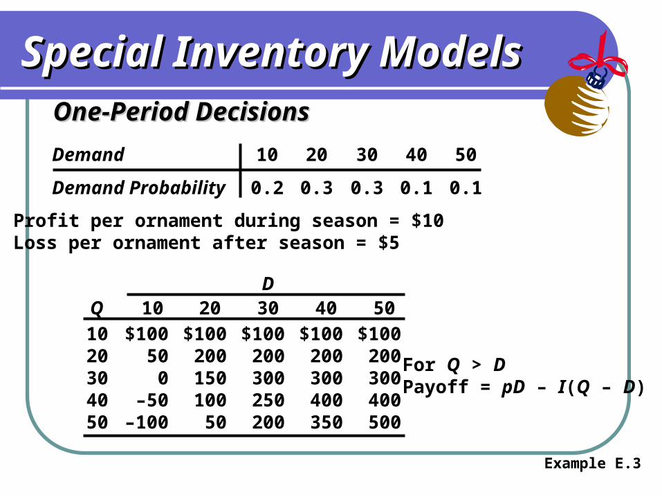
Special Inventory ModelsSpecial Inventory ModelsOne-Period DecisionsOne-Period Decisions

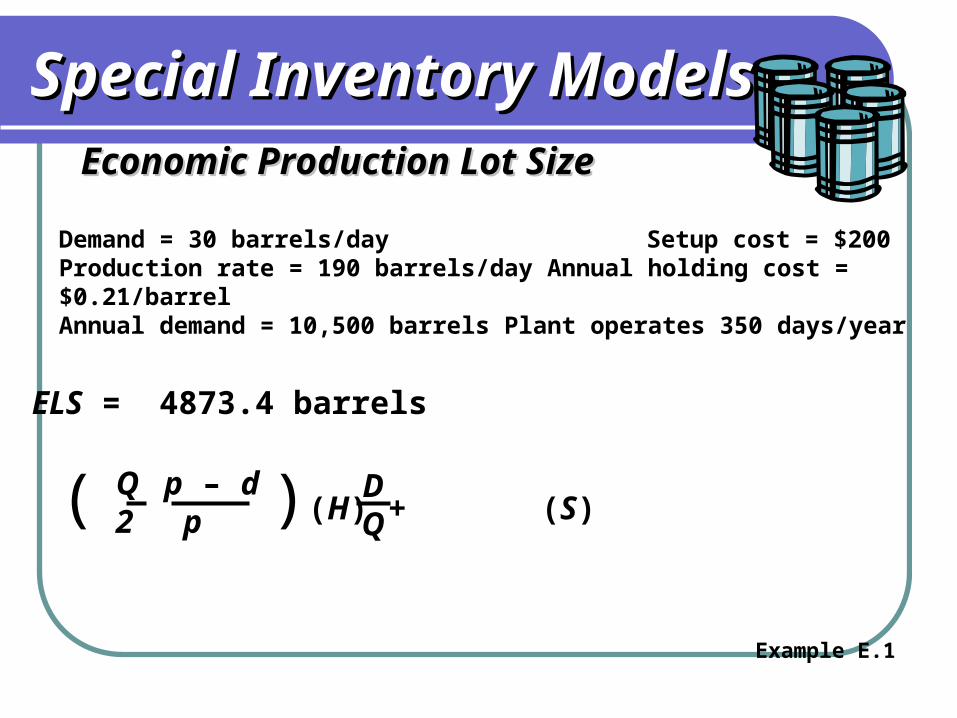
Demand 10 20 30 40 50

Demand Probability 0.2 0.3 0.3 0.1 0.1

Profit per ornament during season = $10Loss per ornament after season = $5

10 $100 $100 $100 $100 $10020304050

DQ 10 20 30 40 50

For Q ≤ DPayoff = pQ

Example E.3


Demand 10 20 30 40 50



10 $100 $100 $100 $100 $10020 200 200 200 20030 300 300 30040 400 40050 500

DQ 10 20 30 40 50

For Q ≤ DPayoff = pQ

Example E.3


Demand 10 20 30 40 50



10 $100 $100 $100 $100 $10020 200 200 200 20030 300 300 30040 400 40050 500

DQ 10 20 30 40 50

For Q > DPayoff = pD – I(Q – D)

Example E.3


Demand 10 20 30 40 50



10 $100 $100 $100 $100 $10020 200 200 200 20030 300 300 30040 400 40050 500

DQ 10 20 30 40 50

For Q > DPayoff = ($10)(30) – ($5)(40 – 30)

Example E.3


Demand 10 20 30 40 50



10 $100 $100 $100 $100 $10020 200 200 200 20030 300 300 30040 250 400 40050 500

DQ 10 20 30 40 50

For Q > DPayoff = $250

Example E.3


Demand 10 20 30 40 50



10 $100 $100 $100 $100 $10020 50 200 200 200 20030 0 150 300 300 30040 –50 100 250 400 40050 –100 50 200 350 500

DQ 10 20 30 40 50

For Q > DPayoff = pD – I(Q – D)

Example E.3


Figure E.5


Demand 10 20 30 40 50



10 $100 $100 $100 $100 $10020 50 200 200 200 20030 0 150 300 300 30040 –50 100 250 400 40050 –100 50 200 350 500

DQ 10 20 30 40 50

Expected payoff30 =

Example E.3


Special Inventory Special Inventory ModelsModelsOne-Period DecisionsOne-Period Decisions

Demand 10 20 30 40 50



10 $100 $100 $100 $100 $10020 50 200 200 200 20030 0 150 300 300 30040 –50 100 250 400 40050 –100 50 200 350 500

DQ 10 20 30 40 50

Expected payoff30 = 0.2($0) + 0.3($150) + 0.3($300) + 0.1($300) + 0.1($300)

Example E.3


Demand 10 20 30 40 50



10 $100 $100 $100 $100 $10020 50 200 200 200 20030 0 150 300 300 300 19540 –50 100 250 400 40050 –100 50 200 350 500

DQ 10 20 30 40 50 Expected Payoff

Expected payoff30 = $195

Example E.3


Demand 10 20 30 40 50



10 $100 $100 $100 $100 $100 $10020 50 200 200 200 200 17030 0 150 300 300 300 19540 –50 100 250 400 400 17550 –100 50 200 350 500 140


Figure E.6


Demand 10 20 30 40 50



10 $100 $100 $100 $100 $100 $10020 50 200 200 200 200 17030 0 150 300 300 300 19540 –50 100 250 400 400 17550 –100 50 200 350 500 140


Figure E.6

Documents

Supplement E - Special Inventory Models. Special Inventory Models Production quantity Demand during production interval Maximum inventory Production and