8623 2020

October 2020

Still in Search of the Sunk Cost Bias Marcello Negrini, Arno Riedl, Matthias Wibral

Impressum:

CESifo Working Papers ISSN 2364-1428 (electronic version) Publisher and distributor: Munich Society for the Promotion of Economic Research - CESifo GmbH The international platform of Ludwigs-Maximilians University’s Center for Economic Studies and the ifo Institute Poschingerstr. 5, 81679 Munich, Germany Telephone +49 (0)89 2180-2740, Telefax +49 (0)89 2180-17845, email office@cesifo.de Editor: Clemens Fuest https://www.cesifo.org/en/wp An electronic version of the paper may be downloaded · from the SSRN website: www.SSRN.com · from the RePEc website: www.RePEc.org · from the CESifo website: https://www.cesifo.org/en/wp

CESifo Working Paper No. 8623

Still in Search of the Sunk Cost Bias

Abstract Evidence from hypothetical scenarios strongly suggests the existence of a sunk cost bias, the tendency to ‘throw good money after bad money.’ However, the few studies using incentives are inconclusive. In addition, evidence on potential psychological channels underlying such a bias is scarce. We present a laboratory experiment designed to investigate the sunk cost bias and to test some prominent psychological mechanisms. Inspired by the hypothetical scenarios, we use a two-stage investment task in which an initial investment needs to be made to start a project. In the initial investment stage, the size of the investment and the responsibility of the investor are exogenously varied. In the second investment stage, participants can either decide to terminate the project or to make an additional investment to finish the project. We do not find evidence for the sunk cost bias. To the contrary, we observe a robust reverse sunk cost bias. That is, the larger the initial investment, the lower the likelihood to continue investing in a project. Moreover, whether or not subjects are responsible for the initial investment, does not affect their additional investment. More waste averse individuals also do not react more strongly to sunk cost whereas being in the loss domain decreases additional investment. Importantly, we replicate the sunk cost bias when using hypothetical scenarios. Surprisingly, the reverse sunk cost bias also holds for those participants who exhibit a strong sunk cost bias in the hypothetical scenarios.

JEL-Codes: C910, D010, D900, D910.

Keywords: sunk cost bias, incentivized experiment, hypothetical scenario, cognitive dissonance, loss aversion, waste aversion.

Marcello Negrini* Maastricht University / The Netherlands

m.negrini@maastrichtuniversity.nl

Arno Riedl Maastricht University / The Netherlands

a.riedl@maastrichtuniversity.nl Matthias Wibral

Maastricht University / The Netherlands m.wibral@maastrichtuniversity.nl

*corresponding author October 2020 The authors thank the Maastricht University – Center for Neuroeconomics (MU-CEN) and the Graduate School of Business and Economics (GSBE) at Maastricht University, for financial support. Matthias Wibral gratefully acknowledges financial support from the European Union’s Horizon 2020 research and innovation programme under the Marie Skłodowska-Curie grant agreement 749741. We thank Andreas Schwaab and Edris Noori for research assistance and Shu Chen for programming the task with z-Tree. We thank the members of the Prague Summer School on Behavioral Economics and Psychology, the members of the MU-CEN and of the Human Decisions & Policy Design research theme (HDPD) at Maastricht University, and seminar participants at the University of Bonn for their comments. We especially thank Andrea Mannberg, Eveline Vandewal, Holger Gerhardt, Peter Werner, Riccardo Saulle and Jona Linde for their insightful feedback, and Nickolas Gagnon for his extensive feedback on an earlier version of this manuscript. This study was preregistered at OSF (https://osf.io/c253e).

1 Introduction

The sunk cost bias refers to the behavioral tendency to continue an endeavor once an investment

has been made, even if it is not optimal to do so (Arkes and Blumer, 1985). The bulk of the

evidence suggesting the existence of the sunk cost bias consists of responses to hypothetical survey

questions (e.g. Arkes and Ayton, 1999; Fox and Staw, 1979; Molden and Hui, 2011; Soman and

Cheema, 2001; Staw, 1976; Strough et al., 2008). For instance, in the seminal paper by Arkes

and Blumer (1985), participants are asked to imagine that they are the owners of a company

and have previously invested a large sum of money in what seemed to be a promising project.

When the project is almost finished, they learn that a competitor is about to release a better

product at a cheaper price. Respondents then need to consider whether to stop investing in the

development of their product and realize the loss or to persist with the project by making an

additional investment. Participants overwhelmingly state to carry out the additional investment

and are thus considered to fall prey to the sunk cost bias.

Examining the sunk cost bias is important because it has been implicated in a wide spectrum

of situations involving sunk costs in practice. For example, the sunk cost bias has been put

forward as an explanation for why politicians continue public works that went over budget (Ross

and Staw, 1993), why firms continue to invest in hopeless projects (Arkes and Blumer, 1985),

why people stay in failing relationships (Strube, 1988), or why researchers continue less promising

projects instead of starting new ones.

Interestingly, despite the intuitive appeal of the concept and the substantial body of evidence

from survey studies, it has been hard to demonstrate the sunk cost bias in incentivized studies,

both in the field and the lab (e.g. Friedman et al., 2007; Ashraf et al., 2010). Existing attempts

to study the sunk cost bias in the laboratory often have quite complicated designs and may be

prone to game form misconceptions (Cason and Plott, 2014), which might explain the incon-

sistent evidence. Therefore, it is important to have a workhorse for studying the bias that is

simple to understand and easily implementable, yet rich enough to allow learning more about the

psychological mechanisms underlying the sunk cost bias.

In this paper we present a novel design with incentivized choices to investigate the sunk

cost bias as well as important potential psychological mechanisms that could drive the bias.1

The experimental design is inspired by the classic project continuation example from the survey

literature. Specifically, we study a two-stage investment task in which an initial investment needs

1The study reported in the paper was preregistered at OSF (https://osf.io/c253e).

1

to be made to start a project and to advance it to a second investment stage. In the second

investment stage, participants know the size of the initial investment size and can either decide

to terminate the project, or to carry out an additional investment to finish the project. If an

additional investment is made, the project is successful and yields a high payoff with some known

probability.

When participants make the decision about the initial investment, the exact cost of the

initial investment are unknown to them, but they do know the distribution of the potential

costs. Participants learn the exact costs of their initial investment only when they have to decide

whether to make the additional investment. The key idea here is that by varying the amount

initially invested (i.e., the sunk cost), we can study the impact of the size of the sunk cost on the

willingness to make the additional investment. A rational decision-maker should ignore the initial

investment and decide whether to make the additional investment based solely on the expected

utility of the available options. If we observe that participants are more willing to make the

additional investment after larger initial investments, this is evidence in favor of the sunk cost

bias.

Our design also includes features that allow us to test several psychological mechanisms that

have been proposed as drivers of the sunk cost bias. Specifically, we examine the roles of re-

sponsibility for the initial investment, of waste aversion, and of being in the loss domain when

making the additional investment decision. Concerning the role of responsibility, self-justification

and cognitive dissonance theory (e.g. Bazerman et al., 1984; Brockner, 1992; Staw, 1976) propose

that abandoning a project after an initial investment requires admitting that the initial invest-

ment was a bad decision. The sunk cost bias arises because continuing to pour resources into a

failing course of action is a way to justify one’s own past decisions. Personal responsibility for the

sunk cost should thus increase the willingness to invest additional resources for the continuation

of a project. To test this, we compare two types of situations, one in which participants are

responsible for the initial investment, and one in which they are not.

Another reason why the sunk cost bias may occur could be waste aversion. Arkes and Blumer

(1985) suggest that people are more willing to invest after bad news because not investing con-

stitutes an admission that the prior expenses were wasted. To investigate this, we include a

questionnaire measure of waste aversion (Haller and Schwabe, 2014). If waste aversion drives

the sunk cost bias, we would expect that more waste averse participants display a stronger sunk

cost bias independent of responsibility for the initial investment. In addition, the effect should

increase with the size of the sunk cost.

2

Our exogenous variation of sunk cost at the individual level also allows us to test whether

the sunk cost bias depends on being in the loss domain. Prospect Theory suggests that the value

function is concave in the gain domain and convex in the loss domain, relatively to a reference

point (Kahneman and Tversky, 1979). According to this S-shaped value function, individuals are

risk seeking in the domain of losses and risk averse in the gain domain. Being in the loss domain

may thus lead to the sunk cost bias because further losses do not result in large decreases in

value; however, comparable gains do result in large increases in value.

There are two additional features of our design. First, it is simple and easy to understand.

As we discuss below, some of the previous work in experimental economics has used relatively

complicated designs which may have confused subjects (Weigel, 2018). Second, we also replicate

classic survey measures of the sunk cost bias from the psychology literature (Arkes and Blumer,

1985) in a post-experimental questionnaire. We can thus compare the results from our incentivized

task to classic survey measures within subject. This comparison can shed light on the discrepancy

of findings between surveys and incentivized studies.

Most of the evidence in favor of the sunk cost bias comes from hypothetical scenarios, whereas

the evidence from incentivized studies is mixed (for reviews, see, e.g., Sleesman et al., 2012;

Roth et al., 2015). To account for the inconsistent evidence, alternative explanations have been

suggested. For instance, responses in hypothetical vignette scenarios that have been interpreted

as a sunk cost bias may actually be due to the fact that participants do not fully adopt the

preferences described in the scenarios, but use their own homegrown preferences (Friedman et al.,

2007).2 In addition, as noted by Weigel (2018), subjects who are indifferent or confused might

exhibit choices that could be misinterpreted as the sunk cost bias.

Regarding field data, three recent papers report evidence that is consistent with a sunk cost

bias. Augenblick (2016) shows that data from penny auctions are in line with the predictions of

a theoretical model in which players’ value of winning the good increases with their previous bid

costs. Ratnadiwakara and Yerramilli (2017) find that past property taxes in California lead to

a significant increase of the sellers’ chosen listing price. Ho et al. (2018) exploit changes in the

price of a government license to buy a car in Singapore and find that an increase in sunk costs

(i.e., the price of the license) leads to an increase in driving.

2For example, a common scenario tells participants that they have accidentally booked vacations for the samedate at two different locations and now have to decide where to go. They are told to imagine that they spent moremoney on location A, but that they actually prefer location B. Choosing location A is interpreted as evidence forthe sunk cost bias. However, if the participant actually prefers A over B and chooses A for this reason then theresponse is not necesarily biased.

3

Attempts to find the sunk cost bias in field experiments have been less successful. Arkes

and Blumer (1985) find that randomly providing discounts to buyers of theatre season tickets

decreases show attendance. However, this effect is only observed for the first half of the theatre

season and the sample is quite small. Ashraf et al. (2010) conducted field experiments testing the

impact of transaction price on the usage of a certain product. They report no evidence of a sunk

cost bias as households paying a higher transaction price are not more likely to use the product.

Ketel et al. (2016) test for a sunk cost bias in an educational setting. Students signing up for

extra-curricular tutorial sessions randomly received a discount on the tuition fee. The authors

find that on average the discount does not affect attendance or performance.

Overall, the picture emerging from field data and field experiments is thus quite mixed. One

potential reason is that it is hard to fully control for the possible confounds of selection, reputation,

and subjective beliefs (Weigel, 2018). Mcafee et al. (2010) also argue that conditioning behavior

on sunk costs could be rationalized, if agents react to sunk costs because of informational content,

reputation, or financial and time constraints.

There are only a few incentivized laboratory experiments investigating the sunk cost bias. To

our knowledge, the first attempt in economics is by Phillips et al. (1991). They study whether

identical lottery tickets are valued differently depending on the price (i.e., the sunk cost) at which

they were bought. Only a quarter of participants value the ticket more as the price increases and

thus exhibit a sunk cost bias, while another quarter of subjects show a reverse sunk cost bias, as

they value the ticket less with an increased price. In additional treatments with opportunities to

learn in a market environment, very few subjects exhibit a sunk cost bias. Heath (1995) studies

investments in a lottery where subjects can invest again in the same lottery when they have lost.

He finds a reverse sunk cost bias when the sum of incremental and sunk cost leads to an overall

loss. Offerman and Potters (2006) show that higher entry fees paid to gain the right to operate

in a market lead some players to set prices in a more collusive way.

The most comprehensive laboratory investigation of the sunk cost bias to date is Friedman

et al. (2007). The authors use a computer game where participants decide whether to keep

digging for a treasure on a virtual island or to incur a cost to move to another island. They only

find a very small sunk cost bias that is inconsistent across treatments with some treatments even

showing a reverse sunk cost bias. Our design is similar in spirit to two recent neuroeconomics

papers (Bogdanov et al., 2017; Haller and Schwabe, 2014). However, these papers use deception

in a way that makes their findings hard to interpret. In their setup, both a rational decision-

4

maker and an individual prone to the sunk cost bias may exhibit the same behavior.3 Haita-Falah

(2017) studies a potential sunk cost bias in a setup in which the channels of loss aversion and

cognitive dissonance cannot drive the effect. She finds weak evidence for a sunk cost bias, which is

significant only for high sunk costs. Similar to Heath (1995), Weigel (2018) studies an individual

decision-making task inspired by penny auctions in which subjects endogenously accumulate

sunk cost. In contrast to Heath (1995), he reports that sunk costs increase the decision maker’s

willingness to continue along an unprofitable course of action. Finally, Ronayne et al. (2020) find

that 23% of participants in an MTurk study who have worked for a ticket for a certain lottery do

not switch to a ticket for a dominant lottery when offered to do so.

Our experiment differs from all previous studies in at least one of the following dimensions.

First, our design allows us to test the impact of different levels of sunk cost within subjects.

Second, it considers both situations where the participant is in the gain domain and situations

in which the participant is in the loss domain, relative to the initial endowment. Third, we use

exogenous variation to test the role of responsibility in a clean way at the individual level. We

have a larger sample per treatment and a simpler design than previous studies.4 Fourth, we are

also able to study the role of waste aversion. Finally, our design differs from previous experimental

studies (except Ashraf 2010 and Ketel et al., 2016) as it allows us to compare the tendency to

exhibit the sunk cost bias in both an incentivized and a hypothetical setting.

Our results can be summarized as follows. First, in contrast to studies using hypothetical

questions and all other incentivized studies (except for Heath, 1995), and in contrast to our pre-

registered hypotheses, we do not observe a sunk cost bias but a reverse sunk cost bias. That

is, the larger the initial investment, the lower the likelihood of continuing to invest in a project.

This result also holds when we only consider those participants who display the sunk cost effect

in the hypothetical choice scenarios. Second, contrary to our hypothesis, we find no difference in

behavior depending on whether subjects are responsible for the initial investment or not. That is,

the reverse sunk cost bias is observed irrespective of whether or not participants are responsible for

the initial investment. Third, contrary to our expectation, we observe that participants are even

3Haller and Schwabe (2014) and Bogdanov et al. (2017) study a setup in which a risky investment projectis sometimes successful immediately after a first investment, and sometimes further investments are needed. Ahigher willingness to make the second investment compared to the first one is taken as evidence for a sunk costbias. However, the true success probabilities and the stated ones differ in a way such that first investments have alower success probability. If subjects learn this over time, then they will be less likely to make the first investmentcompared to the second one even if they do not exhibit a sunk cost bias.

4For example, Friedman et al. (2007) state: “it took us several tries over a period of months to get it [theequilibrium strategy in their experiment] right.” In a replication attempt of Haita-Falah (2017) reported by Weigel(2018), numerous subjects complained that they did not understand the instructions.

5

less willing to continue investing when they find themselves in the loss domain compared to the

gain domain. Fourth, we observe that higher self-reported waste aversion is positively correlated

with the willingness to make the additional investment. However, this effect is not larger for

higher higher levels of sunk cost. Finally, we replicate the findings from the hypothetical scenarios

of Arkes and Blumer (1985). Participants generally exhibit the sunk cost bias in hypothetical

scenarios, and especially when they imagine they were responsible for them. Our reverse sunk

cost bias in the incentivized settings thus does not seem to be due to an idiosyncratic sample.

We do not find support that the sunk cost bias in the hypothetical scenarios translates into a

sunk cost bias in the incentivized investment task. Even those participants who exhibit a strong

sunk cost bias in the hypothetical scenarios show a reverse sunk cost bias in the incentivized

investment task.

The rest of the paper is organized as follows. Section 2 presents the experimental design.

Section 3 describes the pre-registered testable hypotheses. Section 4 shows the experimental

results. Finally, Section 5 discusses the results and limitations of the study and concludes.

2 Experimental design

The main part of the experiment consisted of a repeated choice task comprising two investment

stages, which was followed by a questionnaire and an additional choice task. Instructions were

given prior to the start of each respective part. The questionnaire included questions on sociode-

mographic characteristics, waste aversion, and hypothetical scenarios (adapted from Arkes and

Blumer, 1985) to elicit the sunk cost bias. After the questionnaire, participants played a lottery

choice task developed by Gächter et al. (2007) to measure individual loss aversion. The complete

set of instructions used in the experiment (including screenshots) are provided in Appendix G.

2.1 Investment task

The investment task is framed as investing in a project and is inspired by project continuation

scenarios used in some of the questionnaire studies reporting a sunk cost bias. It consists of two

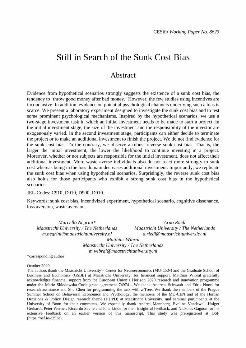
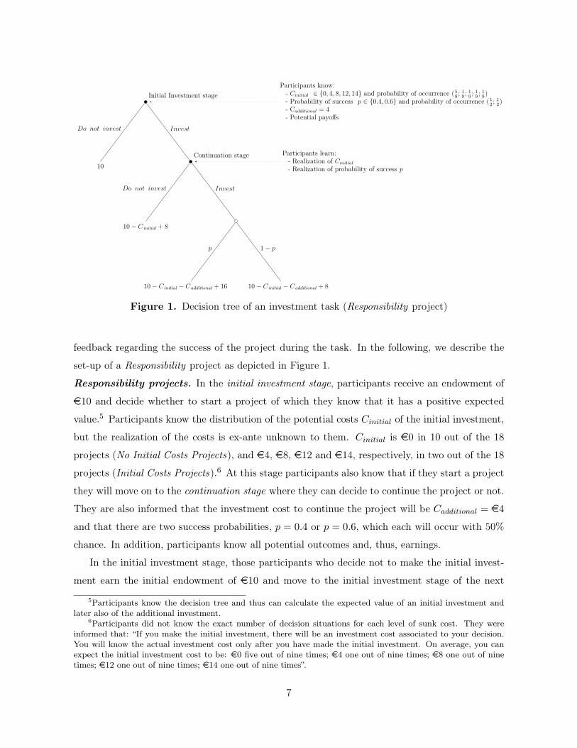
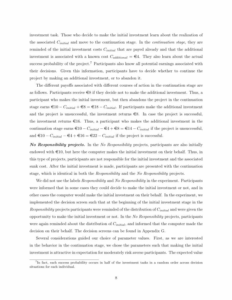
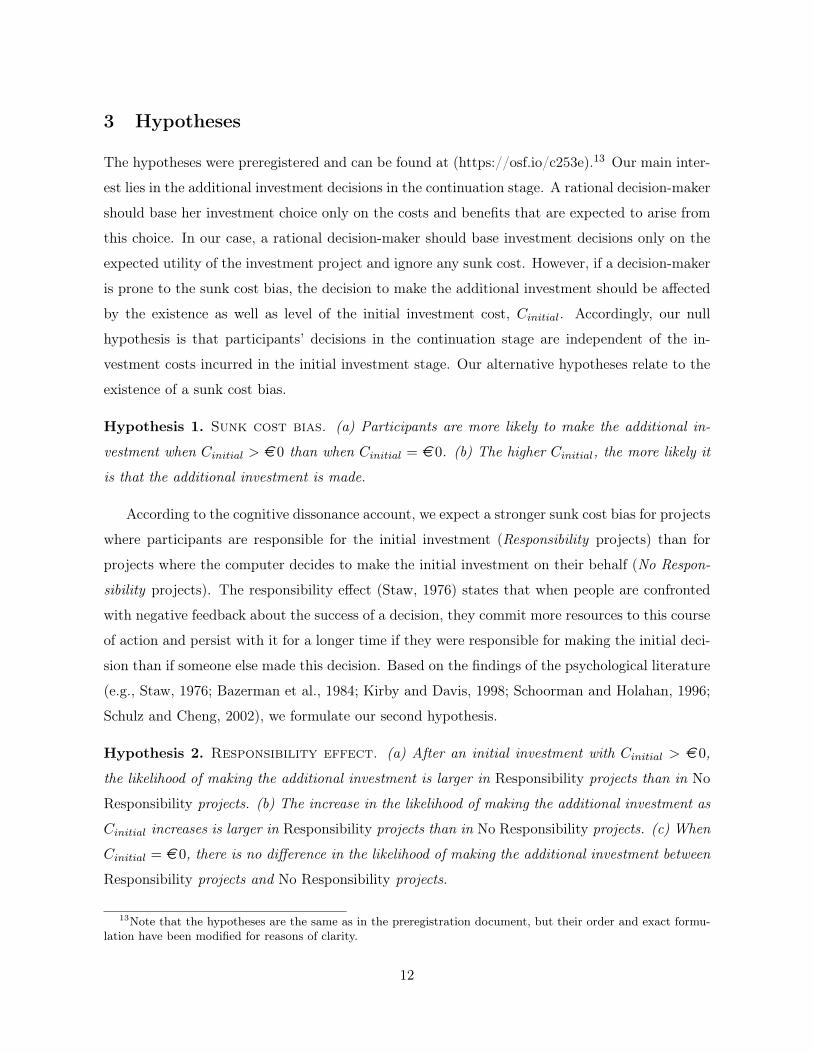
investment stages: an initial investment stage and a continuation stage. Figure 1 provides an

overview of the setup of the investment task. In total, each participant makes decisions in 36

investment tasks, which are evenly split into so-called Responsibility projects and No Responsi-

bility projects. These projects are presented in random order and participants do not receive any

6

Initial Investment stage

10

Doanotainvest Invest

Continuation stage

10− C initial + 8

Doanotainvest Invest

10− C initial − Cadditional + 16aaa

p

aaaa10− C initial − Cadditional + 8

1− p

Participants know:a - Cinitial ∈ {0, 4, 8, 12, 14} and probability of occurrence (5

9 ; 19 ; 1

9 ; 19 ; 1

9)a - Probability of success p ∈ {0.4, 0.6} and probability of occurrence (1

2 ; 12)

a - Cadditional = 4a - Potential payoffs

Participants learn:a - Realization of Cinitial

a - Realization of probability of success p

Figure 1. Decision tree of an investment task (Responsibility project)

feedback regarding the success of the project during the task. In the following, we describe the

set-up of a Responsibility project as depicted in Figure 1.

Responsibility projects. In the initial investment stage, participants receive an endowment of

e10 and decide whether to start a project of which they know that it has a positive expected

value.5 Participants know the distribution of the potential costs Cinitial of the initial investment,

but the realization of the costs is ex-ante unknown to them. Cinitial is e0 in 10 out of the 18

projects (No Initial Costs Projects), and e4, e8, e12 and e14, respectively, in two out of the 18

projects (Initial Costs Projects).6 At this stage participants also know that if they start a project

they will move on to the continuation stage where they can decide to continue the project or not.

They are also informed that the investment cost to continue the project will be Cadditional = e4

and that there are two success probabilities, p = 0.4 or p = 0.6, which each will occur with 50%

chance. In addition, participants know all potential outcomes and, thus, earnings.

In the initial investment stage, those participants who decide not to make the initial invest-

ment earn the initial endowment of e10 and move to the initial investment stage of the next

5Participants know the decision tree and thus can calculate the expected value of an initial investment andlater also of the additional investment.

6Participants did not know the exact number of decision situations for each level of sunk cost. They wereinformed that: “If you make the initial investment, there will be an investment cost associated to your decision.You will know the actual investment cost only after you have made the initial investment. On average, you canexpect the initial investment cost to be: e0 five out of nine times; e4 one out of nine times; e8 one out of ninetimes; e12 one out of nine times; e14 one out of nine times”.

7

investment task. Those who decide to make the initial investment learn about the realization of

the associated Cinitial and move to the continuation stage. In the continuation stage, they are

reminded of the initial investment costs Cinitial that are payed already and that the additional

investment is associated with a known cost Cadditional = e4. They also learn about the actual

success probability of the project.7 Participants also know all potential earnings associated with

their decisions. Given this information, participants have to decide whether to continue the

project by making an additional investment, or to abandon it.

The different payoffs associated with different courses of action in the continuation stage are

as follows. Participants receive e8 if they decide not to make the additional investment. Thus, a

participant who makes the initial investment, but then abandons the project in the continuation

stage earns e10− Cinitial + e8 = e18− Cinitial. If participants make the additional investment

and the project is unsuccessful, the investment returns e8. In case the project is successful,

the investment returns e16. Thus, a participant who makes the additional investment in the

continuation stage earns e10− Cinitial −e4 +e8 = e14− Cinitial if the project is unsuccessful,

and e10− Cinitial − e4 + e16 = e22− Cinitial if the project is successful.

No Responsibility projects. In the No Responsibility projects, participants are also initially

endowed with e10, but here the computer makes the initial investment on their behalf. Thus, in

this type of projects, participants are not responsible for the initial investment and the associated

sunk cost. After the initial investment is made, participants are presented with the continuation

stage, which is identical in both the Responsibility and the No Responsibility projects.

We did not use the labels Responsibility and No Responsibility in the experiment. Participants

were informed that in some cases they could decide to make the initial investment or not, and in

other cases the computer would make the initial investment on their behalf. In the experiment, we

implemented the decision screen such that at the beginning of the initial investment stage in the

Responsibility projects participants were reminded of the distribution of Cinitial and were given the

opportunity to make the initial investment or not. In the No Responsibility projects, participants

were again reminded about the distribution of Cinitial, and informed that the computer made the

decision on their behalf. The decision screens can be found in Appendix G.

Several considerations guided our choice of parameter values. First, as we are interested

in the behavior in the continuation stage, we chose the parameters such that making the initial

investment is attractive in expectation for moderately risk averse participants. The expected value

7In fact, each success probability occurs in half of the investment tasks in a random order across decisionsituations for each individual.

8

of making the initial investment is e14.18 and thus substantially higher than the endowment of

e10. Ex-ante only someone with very strong risk aversion should not make the initial investment.8

We chose the distribution of Cinitial (i.e., the sunk cost) such that the probability of Cinitial = 0

is above 50% with the goal to make the initial investment decision attractive, while at the same

time still having a fairly equal number of observations with Cinitial > 0.

Second, we chose the different levels of the sunk cost such that for half of the decision situations

in which there is a strictly positive sunk cost, abandoning the project in the continuation stage

does not lead to a loss compared to the endowment. For Cinitial of e4, participants who decide to

abandon the project in the continuation stage receive a payoff of e14 and are better off than if they

had not made the initial investment and received their endowment of e10. For a Cinitial of e8,

they break exactly even. For the other two levels of Cinitial (e12 and e14), participants make a

loss compared to their endowment if they decide to abandon the project. These values were chosen

such that assuming a reference point of e10, given the median estimated curvature parameters,

loss aversion coefficient, and probability weighting values from Tversky and Kahneman (1992),

Cumulative Prospect Theory would predict the following: a participant will make the additional

investment with success probability p ≥ 0.4 only for Cinitial ≥ e12.9 Third, we chose to have

two different success probabilities in the continuation stage to minimize possible floor and ceiling

effects, thus having a greater chance of finding a sunk cost bias.

2.2 Psychological measures related to the sunk cost bias

Waste aversion has been proposed as an explanation for the sunk cost bias (Arkes and Blumer,

1985). To explore this mechanism, we ask participants fill out a short questionnaire (Haller and

Schwabe, 2014) that aims to assess their desire not to waste resources after the investment task.

This questionnaire consists of four statements that are answered on a scale from 1 (“I do not

agree”) to 11 (“I completely agree): “It is important for me not to appear wasteful”, “Wasted

investments hurt me”, “People who know me think I am wasteful” (inversely coded), and “It

8For example, any decision maker with the CRRA utility function U(x) = 11−rx

1−r with an r < 2.05 willalways make the initial investment. For comparison, Holt and Laury (2002) do not observe any participant withr > 1.37.

9 We apply Cumulative Prospect Theory as in Tversky and Kahneman (1992), where the prospect is the

product of decision weights π(p) and value of the potential outcome, as shown by: V (x) =

{xα if x ≥ 0

−λ(−x)β if x < 0.

We assume a reference point of e10 (i.e., the initial endowment) and the parameters as estimated in Tversky andKahneman (1992) of loss aversion λ = −2.25, curvature coefficients in the positive domain (α) and in the negativedomain (β) = 0.88, and a decision weight π(p) = ργ

(ργ+(1−ρ)γ)1γ

with γ = 0.61 in the gain domain and γ = 0.69 in

the loss domain.

9

annoys me if investments are not successful”. The scores for the 4 items are summed up and the

total score is taken as an indicator of the strength of the individual’s desire not to appear wasteful.

With our design, we can disentangle the role of waste aversion from cognitive dissonance as its

effect should be present both with and without responsibility for incurring sunk costs, whereas

cognitive dissonance should only affect behavior in the Responsibility projects.

To examine whether the survey measure of the sunk cost bias used in the literature correlates

with our incentivized measure, participants also answer four binary hypothetical questions related

to the sunk cost bias. These questions are slightly modified versions of four vignette studies in the

seminal paper by Arkes and Blumer (1985). To make them more relatable to our subject pool,

we changed the travel destinations and the monetary amounts used in the hypothetical scenarios.

The scenarios are reported in full in Appendix F. For two scenarios, participants were instructed

to imagine they were responsible for the initial investment, while for the other two scenarios they

were told someone else was responsible for it. From the answers, we construct an index ranging

from 0 to 4 indicating the strength of the tendency to show the sunk cost bias in hypothetical

scenarios.

2.3 Loss aversion

To measure loss aversion, we use a task by Gächter et al. (2007).10 In this task, participants

decide for each of six lotteries whether they want to accept it or reject it. Across lotteries, the

winning prize is fixed at e6 while the potential loss varies between e2 and e7, as shown in

Table D.1 in Appendix D.

Under Cumulative Prospect Theory, behavior in this task is jointly determined by probability

weighting, the curvatures of the utility function in the gain and loss domain, and loss aversion.

Under certain assumptions, in particular, linearity of the value function, the task provides a

simple measure of the loss aversion parameter in cumulative prospect theory.11 In the context of

the sunk cost bias, the linearity assumption can influence predictions substantially. For example,

10To keep the experiment within reasonable time limits, we decided against a full-blown estimation of theparameters of a prospect theoretic utility function (e.g., Sokol-Hessner et al., 2009)

11Gächter et al. (2007) assume that a participant is indifferent between accepting and rejecting the lottery ifw

+

(0.5)v(G) = w−(0.5)λ v(L), where L denotes the loss in a given lottery and G the gain; v(x) is the utility of theoutcome x ∈ {G,L}, λ denotes the coefficient of loss aversion in the choice task; and w

+

(0.5) and w−(0.5) denote

the probability weights for the 0.50 chance of gaining G or losing L, respectively. Considering that w+

(0.5) =

w−(0.5), only the ratio v(G)

v(L)= λ defines an individual’s implied loss aversion in the lottery choice task. The

additional assumption that v(x) is linear (v(x) = x) for small amounts yields a very simple measure of lossaversion: λ = G/L.

10

a loss averse individual who does not weight probabilities and has a linear value function will not

display a sunk cost bias in our experiment. In fact, for a sufficiently high degree of loss aversion

(λ > 2), such an individual would be less likely to make the additional investment around their

reference point than when all outcomes lie either in the gain or in the loss domain. In contrast,

another individual with the median cumulative prospect theory parameter values estimated in

Tversky and Kahneman (1992) would show an identical choice pattern in our loss aversion task

as the previous individual, but display a sunk cost bias in the investment task.12

In keeping with the convention, we call the switching point between acceptance and rejection

of the lottery “Loss aversion”, but the reader should be aware that this switching point might

also reflect factors other than loss aversion such as probability weighting and curvature. We also

ran all analyses using the loss aversion λ coefficient as calculated by Gächter et al. (2007), i.e.,

assuming that the value function is linear, instead of the switching point between acceptance and

rejection lottery. All results are qualitatively robust to this alternative specification.

2.4 Procedure

We recruited 108 participants (42 men; mean age = 21.5 years, s.d. =2.5 years) using ORSEE

(Greiner, 2015). The experiment was programmed with z-Tree (Fischbacher, 2007) and conducted

at the Behavioral and Experimental Economics Laboratory (BEELab) of Maastricht University.

Each participant completed the experiment in a randomly assigned cubicle isolated from other

participants. In total, we conducted five experimental sessions and each session lasted about

60 minutes. Each participant completed the incentivized investment task first, followed by the

psychological measures and finally by the loss aversion task. At the end of the experiment, one

randomly selected decision of the investment task and one randomly selected decision in the loss

aversion task counted for payment. Participants were informed that any losses in the loss aversion

task would be deducted from a flat fee of e7 they earned for answering the questionnaire and

the hypothetical questions reported in Section 2.2. During the investment task, participants did

not know that there would be other tasks or payments later in the experiment. Participants

earned e13.75 on average and all earnings were paid via bank transfers, a common procedure in

the Netherlands. Subjects were truthfully informed that the payments were issued by research

assistants unrelated to the experiment and subsequent data analysis, and that their anonymity

was thus assured.

12Such an individual would always make the additional investment for Cinitial ≥ 12, but not for Cinitial < 12,assuming a reference point of 10, i.e., the initial endowment (see Footnote 9).

11

3 Hypotheses

The hypotheses were preregistered and can be found at (https://osf.io/c253e).13 Our main inter-

est lies in the additional investment decisions in the continuation stage. A rational decision-maker

should base her investment choice only on the costs and benefits that are expected to arise from

this choice. In our case, a rational decision-maker should base investment decisions only on the

expected utility of the investment project and ignore any sunk cost. However, if a decision-maker

is prone to the sunk cost bias, the decision to make the additional investment should be affected

by the existence as well as level of the initial investment cost, Cinitial. Accordingly, our null

hypothesis is that participants’ decisions in the continuation stage are independent of the in-

vestment costs incurred in the initial investment stage. Our alternative hypotheses relate to the

existence of a sunk cost bias.

Hypothesis 1. Sunk cost bias. (a) Participants are more likely to make the additional in-

vestment when Cinitial > e 0 than when Cinitial = e 0. (b) The higher Cinitial, the more likely it

is that the additional investment is made.

According to the cognitive dissonance account, we expect a stronger sunk cost bias for projects

where participants are responsible for the initial investment (Responsibility projects) than for

projects where the computer decides to make the initial investment on their behalf (No Respon-

sibility projects). The responsibility effect (Staw, 1976) states that when people are confronted

with negative feedback about the success of a decision, they commit more resources to this course

of action and persist with it for a longer time if they were responsible for making the initial deci-

sion than if someone else made this decision. Based on the findings of the psychological literature

(e.g., Staw, 1976; Bazerman et al., 1984; Kirby and Davis, 1998; Schoorman and Holahan, 1996;

Schulz and Cheng, 2002), we formulate our second hypothesis.

Hypothesis 2. Responsibility effect. (a) After an initial investment with Cinitial > e 0,

the likelihood of making the additional investment is larger in Responsibility projects than in No

Responsibility projects. (b) The increase in the likelihood of making the additional investment as

Cinitial increases is larger in Responsibility projects than in No Responsibility projects. (c) When

Cinitial = e 0, there is no difference in the likelihood of making the additional investment between

Responsibility projects and No Responsibility projects.

13Note that the hypotheses are the same as in the preregistration document, but their order and exact formu-lation have been modified for reasons of clarity.

12

Conditional on finding that participants exhibit a sunk cost bias, we formulate further hy-

potheses relating to potential mechanisms behind the sunk cost bias. If the desire not to waste

resources or not to appear wasteful drives the sunk cost effect (Arkes and Blumer, 1985), we

expect that waste aversion correlates with the sunk cost bias.

Hypothesis 3. Waste aversion. (a) The higher the initial investment cost, the more the

waste aversion score positively correlates with the likelihood of making the additional investment.

(b) Hypothesis 2(c) is confirmed and, after initial investment when Cinitial > e 0, there is no

difference in the likelihood of making an additional investment between Responsibility and No

Responsibility projects.

The sunk cost bias may emerge when participants fall behind their initial endowment of e10.

That is, when they are in the loss domain relative to this endowment. Recall that, for projects

with Cinitial of e12 and e14, participants who do not make an additional investment fall behind

the initial endowment for sure, because in that case they only earn e6 and e4, respectively. Thus,

based on Cumulative Prospect Theory (see Footnote 9) we formulate the following hypothesis.

Hypothesis 4. Loss domain (a) The likelihood of making the additional investment when

Cinitial is e12 or e14 is higher than for lower non-zero initial investment costs. (b) This differ-

ence in the likelihood of making the additional investment is positively related to the loss aversion

score.

4 Results

In this section, we describe our findings in relation to the preregistered hypotheses. When a

hypothesis is rejected, we present additional exploratory analyses. First, we investigate whether

we find evidence of a sunk cost bias. Second, we describe the influence of responsibility for the

sunk costs on the willingness to continue to invest. Third, we investigate the impact of waste

aversion, and of being in the loss domain. Finally, we show whether the tendency to exhibit a

sunk cost in a hypothetical setting is correlated with the findings in the incentivized setting.

We present results using both non-parametric tests and regression analyses. All reported tests

are two-sided. In the regression analyses, we use logit models with standard errors clustered at the

participant level. The dependent variable is the decision to make the additional investment in the

continuation stage, coded as a binary variable taking on value 1 when the additional investment

was made and value 0 when it was not made. Depending on the hypotheses considered, the sunk

13

costs are coded in three different ways: (1) as a dummy variable that takes on value 1 when the

initial investment cost is strictly positive (called Initial Cost > 0 ), (2) as a continuous variable

with the values of Cinitial (called Initial Cost), and (3) as a dummy variable that takes on value

1 if Cinitial is e12 or e14 (called Loss Domain).

In the presentation of regression results we focus on those specifications where control variables

are included, but also report the results without control variables for completeness. Control

variables comprise the probability of project success, the measure of loss aversion and waste

aversion, the score in the hypothetical sunk cost questionnaire, gender, whether the field of study

is economics, and the repetitions of trials in the task, unless otherwise specified.14 The coefficient

estimates of the control variable estimates are reported in Appendix A.

4.1 Is there evidence of a sunk cost bias?

According to the sunk cost hypothesis, we expected that participants should be more likely to

make the additional investment with Cinitial > e 0 (Hypothesis 1a). We also expected that the

higher Cinitial, the more likely a participant is to make the additional investment (Hypothe-

sis 1b). In contrast, however, we observe that participants are less willing to make the additional

investment when Cinitial > e 0 (61%) compared to when Cinitial = e 0 (79%). This difference in

the relative frequency of investment choices in the continuation stage is statistically significant

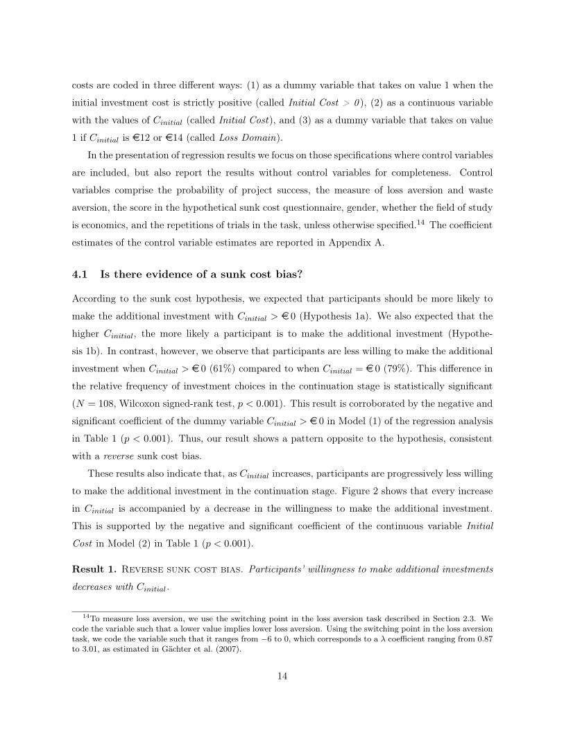
(N = 108, Wilcoxon signed-rank test, p < 0.001). This result is corroborated by the negative and

significant coefficient of the dummy variable Cinitial > e 0 in Model (1) of the regression analysis

in Table 1 (p < 0.001). Thus, our result shows a pattern opposite to the hypothesis, consistent

with a reverse sunk cost bias.

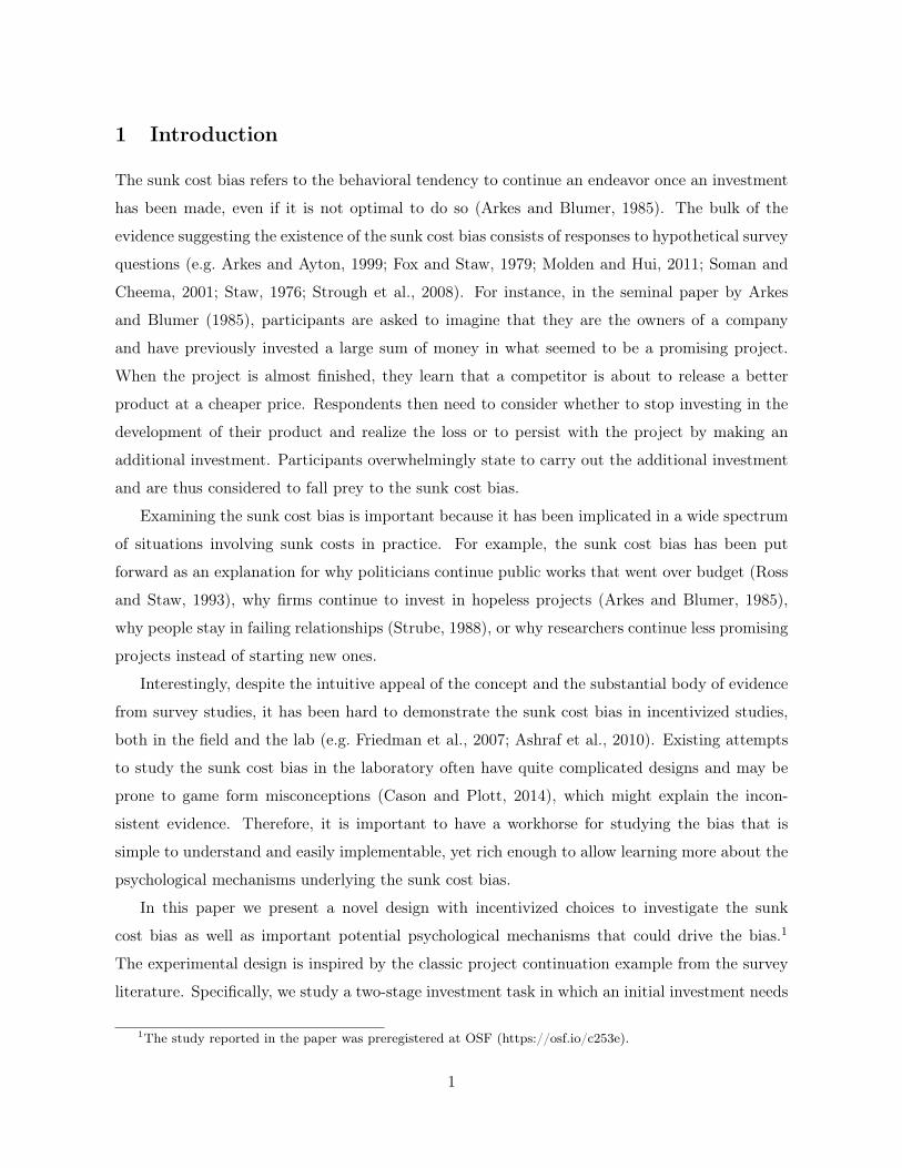
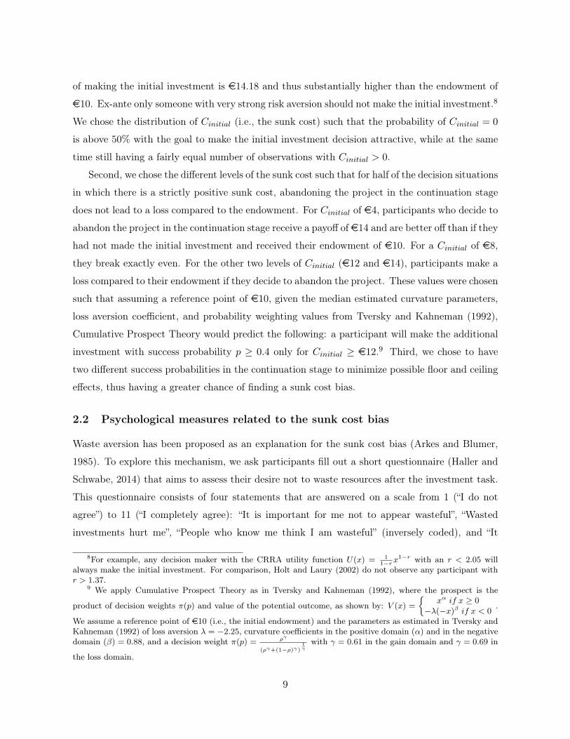
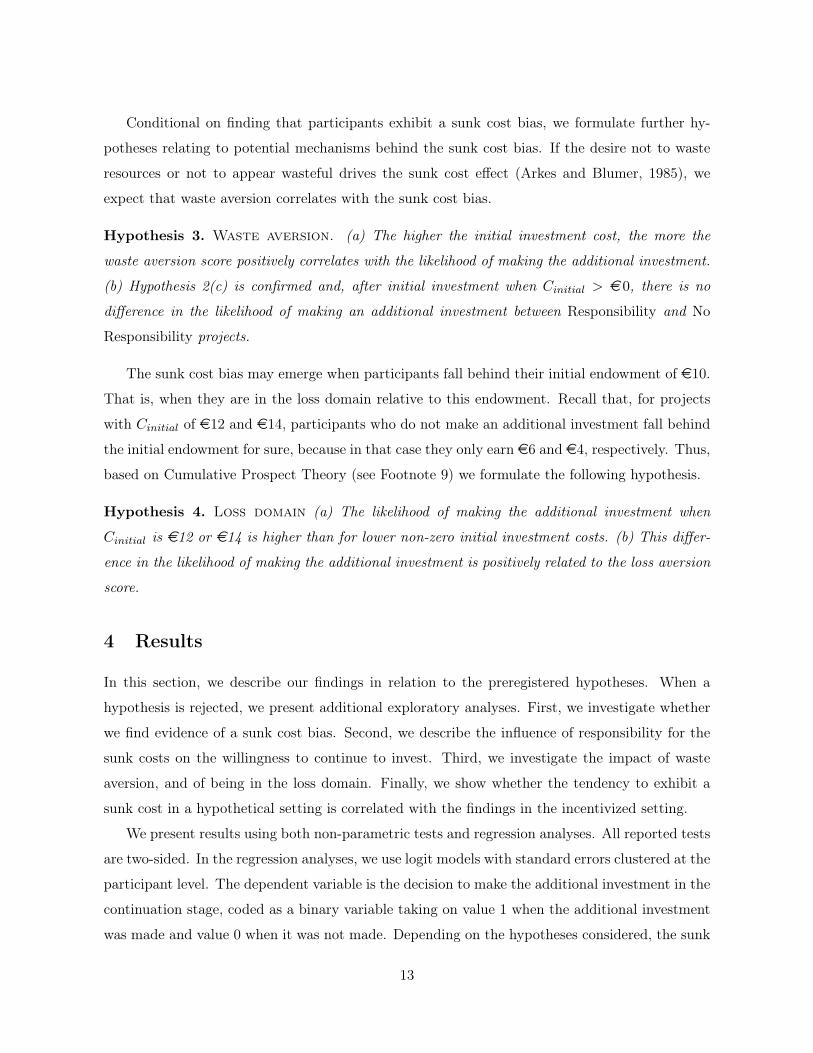
These results also indicate that, as Cinitial increases, participants are progressively less willing

to make the additional investment in the continuation stage. Figure 2 shows that every increase

in Cinitial is accompanied by a decrease in the willingness to make the additional investment.

This is supported by the negative and significant coefficient of the continuous variable Initial

Cost in Model (2) in Table 1 (p < 0.001).

Result 1. Reverse sunk cost bias. Participants’ willingness to make additional investments

decreases with Cinitial.

14To measure loss aversion, we use the switching point in the loss aversion task described in Section 2.3. Wecode the variable such that a lower value implies lower loss aversion. Using the switching point in the loss aversiontask, we code the variable such that it ranges from −6 to 0, which corresponds to a λ coefficient ranging from 0.87to 3.01, as estimated in Gächter et al. (2007).

14

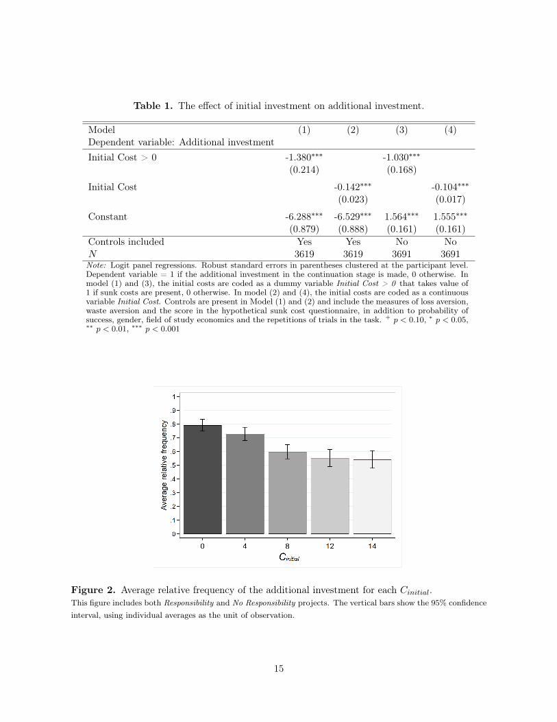
Table 1. The effect of initial investment on additional investment.

Model (1) (2) (3) (4)Dependent variable: Additional investmentInitial Cost > 0 -1.380∗∗∗ -1.030∗∗∗

(0.214) (0.168)

Initial Cost -0.142∗∗∗ -0.104∗∗∗

(0.023) (0.017)

Constant -6.288∗∗∗ -6.529∗∗∗ 1.564∗∗∗ 1.555∗∗∗

(0.879) (0.888) (0.161) (0.161)Controls included Yes Yes No NoN 3619 3619 3691 3691Note: Logit panel regressions. Robust standard errors in parentheses clustered at the participant level.Dependent variable = 1 if the additional investment in the continuation stage is made, 0 otherwise. Inmodel (1) and (3), the initial costs are coded as a dummy variable Initial Cost > 0 that takes value of1 if sunk costs are present, 0 otherwise. In model (2) and (4), the initial costs are coded as a continuousvariable Initial Cost. Controls are present in Model (1) and (2) and include the measures of loss aversion,waste aversion and the score in the hypothetical sunk cost questionnaire, in addition to probability ofsuccess, gender, field of study economics and the repetitions of trials in the task. + p < 0.10, ∗ p < 0.05,∗∗ p < 0.01, ∗∗∗ p < 0.001

Figure 2. Average relative frequency of the additional investment for each Cinitial.This figure includes both Responsibility and No Responsibility projects. The vertical bars show the 95% confidenceinterval, using individual averages as the unit of observation.

15

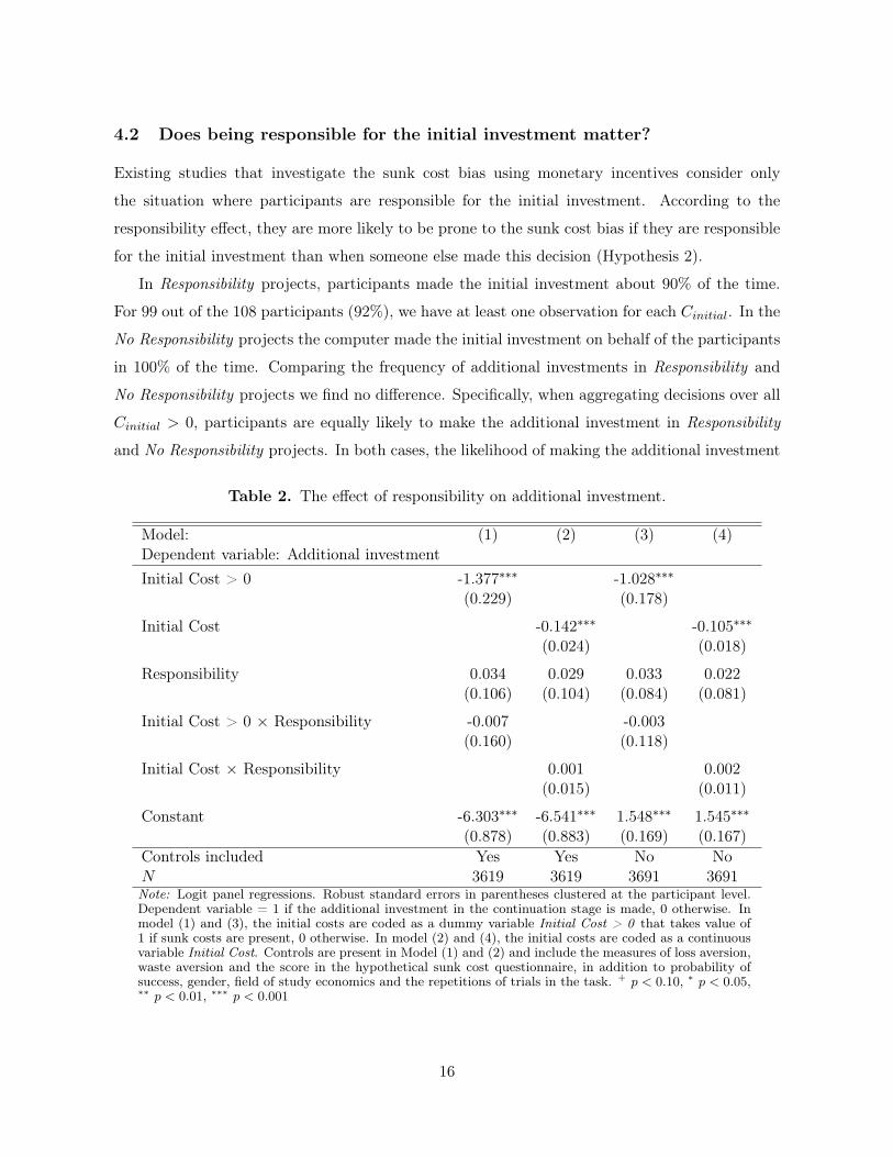
4.2 Does being responsible for the initial investment matter?

Existing studies that investigate the sunk cost bias using monetary incentives consider only

the situation where participants are responsible for the initial investment. According to the

responsibility effect, they are more likely to be prone to the sunk cost bias if they are responsible

for the initial investment than when someone else made this decision (Hypothesis 2).

In Responsibility projects, participants made the initial investment about 90% of the time.

For 99 out of the 108 participants (92%), we have at least one observation for each Cinitial. In the

No Responsibility projects the computer made the initial investment on behalf of the participants

in 100% of the time. Comparing the frequency of additional investments in Responsibility and

No Responsibility projects we find no difference. Specifically, when aggregating decisions over all

Cinitial > 0, participants are equally likely to make the additional investment in Responsibility

and No Responsibility projects. In both cases, the likelihood of making the additional investment

Table 2. The effect of responsibility on additional investment.

Model: (1) (2) (3) (4)Dependent variable: Additional investmentInitial Cost > 0 -1.377∗∗∗ -1.028∗∗∗

(0.229) (0.178)

Initial Cost -0.142∗∗∗ -0.105∗∗∗

(0.024) (0.018)

Responsibility 0.034 0.029 0.033 0.022(0.106) (0.104) (0.084) (0.081)

Initial Cost > 0 × Responsibility -0.007 -0.003(0.160) (0.118)

Initial Cost × Responsibility 0.001 0.002(0.015) (0.011)

Constant -6.303∗∗∗ -6.541∗∗∗ 1.548∗∗∗ 1.545∗∗∗

(0.878) (0.883) (0.169) (0.167)Controls included Yes Yes No NoN 3619 3619 3691 3691Note: Logit panel regressions. Robust standard errors in parentheses clustered at the participant level.Dependent variable = 1 if the additional investment in the continuation stage is made, 0 otherwise. Inmodel (1) and (3), the initial costs are coded as a dummy variable Initial Cost > 0 that takes value of1 if sunk costs are present, 0 otherwise. In model (2) and (4), the initial costs are coded as a continuousvariable Initial Cost. Controls are present in Model (1) and (2) and include the measures of loss aversion,waste aversion and the score in the hypothetical sunk cost questionnaire, in addition to probability ofsuccess, gender, field of study economics and the repetitions of trials in the task. + p < 0.10, ∗ p < 0.05,∗∗ p < 0.01, ∗∗∗ p < 0.001

16

was 60.5% (N = 107; Wilcoxon signed-rank test, p = 0.546).15 This result is corroborated in

the regression analysis of Model (1) in Table 2 by the insignificant coefficient of the interaction

between Initial Cost > 0 and a dummy variable Responsibility which takes value 1 when the

participant is responsible for making the initial investment (p = 0.965). This indicates that,

when Cinitial > e0, there is no difference in the likelihood of making an additional investment

between Responsibility and No Responsibility projects. Hypothesis 2a is thus rejected.

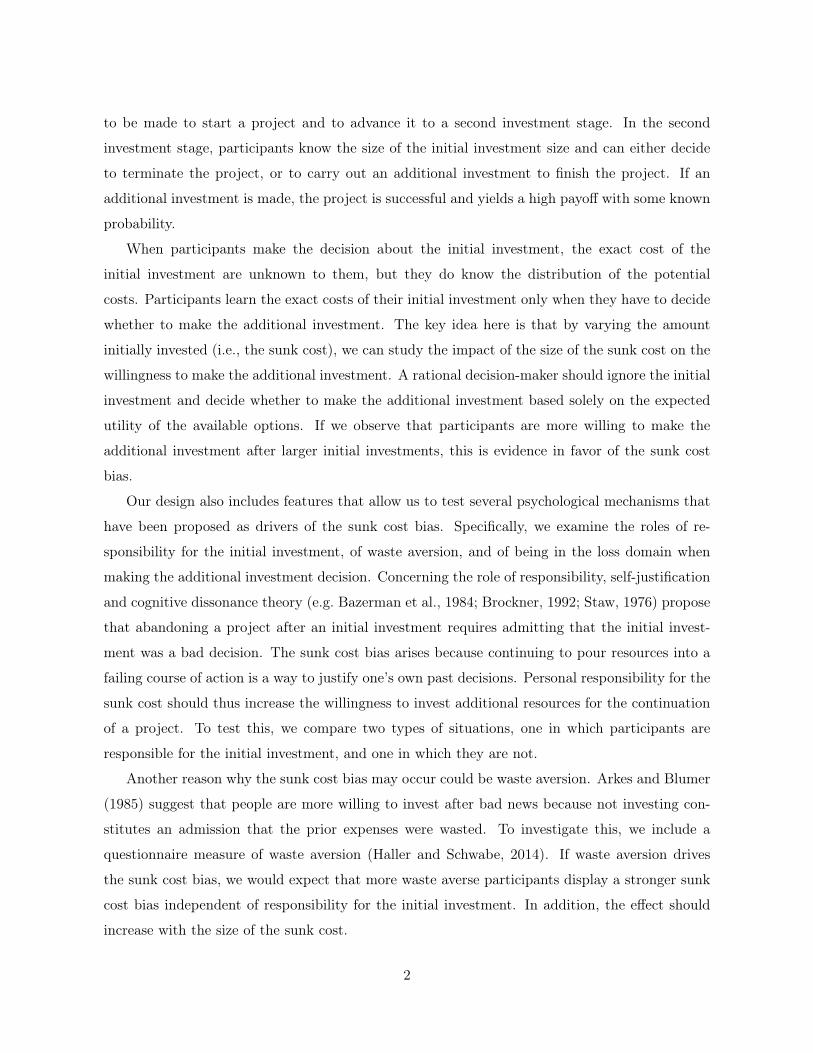
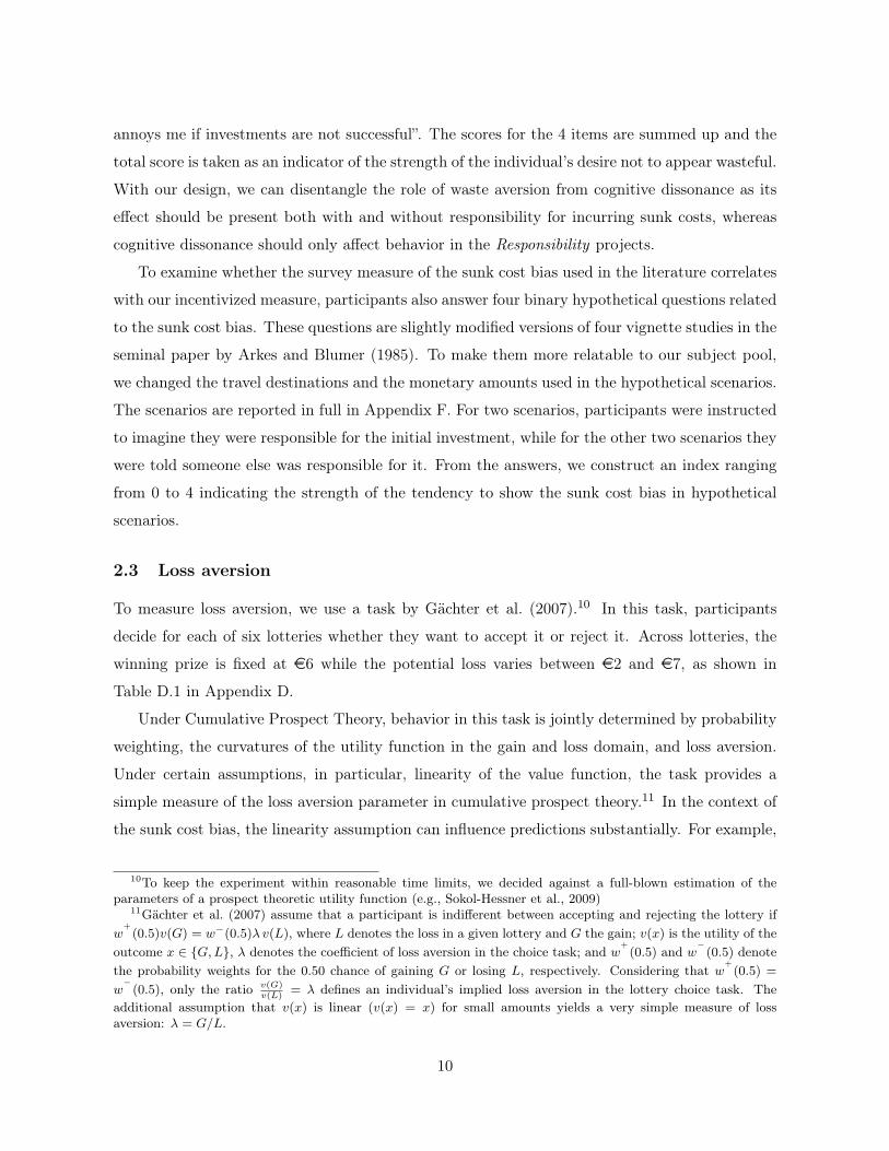
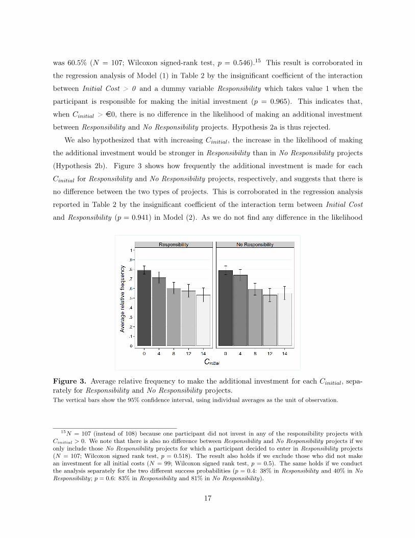
We also hypothesized that with increasing Cinitial, the increase in the likelihood of making

the additional investment would be stronger in Responsibility than in No Responsibility projects

(Hypothesis 2b). Figure 3 shows how frequently the additional investment is made for each

Cinitial for Responsibility and No Responsibility projects, respectively, and suggests that there is

no difference between the two types of projects. This is corroborated in the regression analysis

reported in Table 2 by the insignificant coefficient of the interaction term between Initial Cost

and Responsibility (p = 0.941) in Model (2). As we do not find any difference in the likelihood

Figure 3. Average relative frequency to make the additional investment for each Cinitial, sepa-rately for Responsibility and No Responsibility projects.The vertical bars show the 95% confidence interval, using individual averages as the unit of observation.

15N = 107 (instead of 108) because one participant did not invest in any of the responsibility projects withCinitial > 0. We note that there is also no difference between Responsibility and No Responsibility projects if weonly include those No Responsibility projects for which a participant decided to enter in Responsibility projects(N = 107; Wilcoxon signed rank test, p = 0.518). The result also holds if we exclude those who did not makean investment for all initial costs (N = 99; Wilcoxon signed rank test, p = 0.5). The same holds if we conductthe analysis separately for the two different success probabilities (p = 0.4: 38% in Responsibility and 40% in NoResponsibility ; p = 0.6: 83% in Responsibility and 81% in No Responsibility).

17

of making the additional investment between Responsibility and No Responsibility as Cinitial

increases, we thus reject Hypothesis 2b.16

Finally, we hypothesized that participants would be equally likely to make the additional

investment in Responsibility and No Responsibility projects when Cinitial is zero (Hypothesis 2c).

A Wilcoxon signed-rank test supports this hypothesis (N = 108; p = 0.785), which is corroborated

by the insignificant coefficient of the variable Responsibility in Model (1) in Table 2 (p = 0.747).17

Result 2. Responsibility effect. Responsibility for the initial investment does not signifi-

cantly influence the likelihood of making the additional investment.

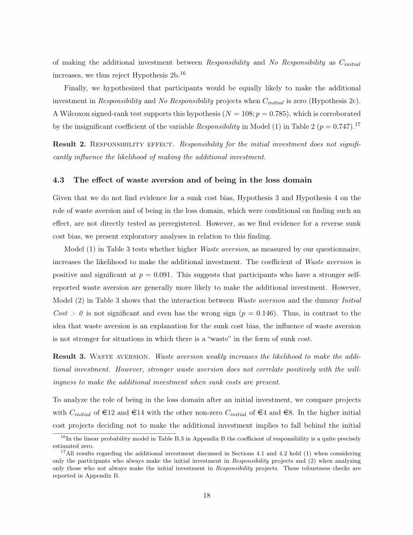
4.3 The effect of waste aversion and of being in the loss domain

Given that we do not find evidence for a sunk cost bias, Hypothesis 3 and Hypothesis 4 on the

role of waste aversion and of being in the loss domain, which were conditional on finding such an

effect, are not directly tested as preregistered. However, as we find evidence for a reverse sunk

cost bias, we present exploratory analyses in relation to this finding.

Model (1) in Table 3 tests whether higher Waste aversion, as measured by our questionnaire,

increases the likelihood to make the additional investment. The coefficient of Waste aversion is

positive and significant at p = 0.091. This suggests that participants who have a stronger self-

reported waste aversion are generally more likely to make the additional investment. However,

Model (2) in Table 3 shows that the interaction between Waste aversion and the dummy Initial

Cost > 0 is not significant and even has the wrong sign (p = 0.146). Thus, in contrast to the

idea that waste aversion is an explanation for the sunk cost bias, the influence of waste aversion

is not stronger for situations in which there is a “waste” in the form of sunk cost.

Result 3. Waste aversion. Waste aversion weakly increases the likelihood to make the addi-

tional investment. However, stronger waste aversion does not correlate positively with the will-

ingness to make the additional investment when sunk costs are present.

To analyze the role of being in the loss domain after an initial investment, we compare projects

with Cinitial of e12 and e14 with the other non-zero Cinitial of e4 and e8. In the higher initial

cost projects deciding not to make the additional investment implies to fall behind the initial16In the linear probability model in Table B.3 in Appendix B the coefficient of responsibility is a quite precisely

estimated zero.17All results regarding the additional investment discussed in Sections 4.1 and 4.2 hold (1) when considering

only the participants who always make the initial investment in Responsibility projects and (2) when analyzingonly those who not always make the initial investment in Responsibility projects. These robustness checks arereported in Appendix B.

18

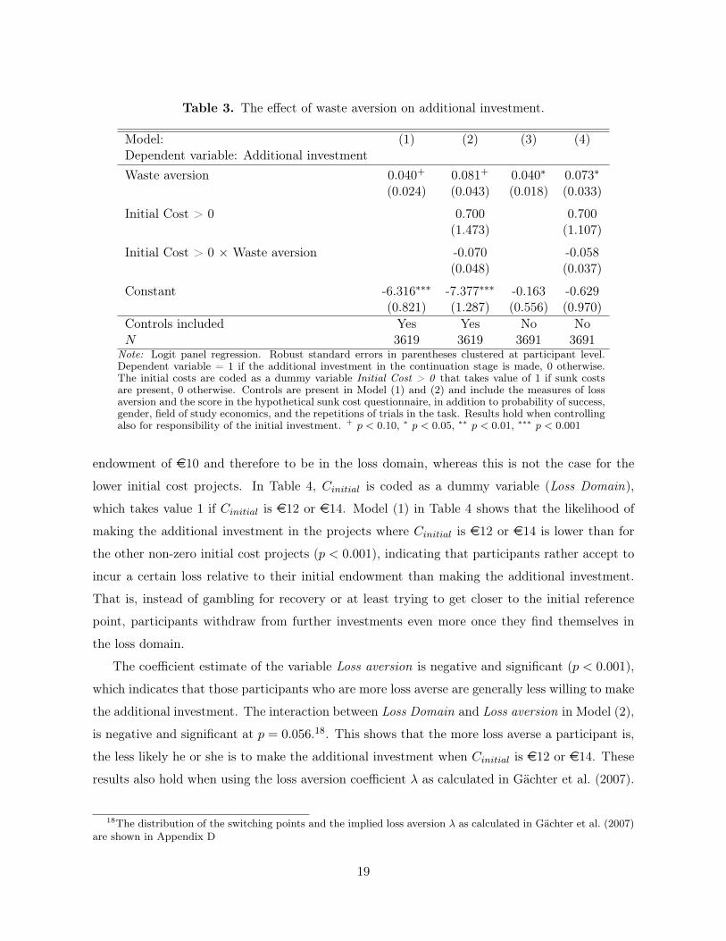
Table 3. The effect of waste aversion on additional investment.

Model: (1) (2) (3) (4)Dependent variable: Additional investmentWaste aversion 0.040+ 0.081+ 0.040∗ 0.073∗

(0.024) (0.043) (0.018) (0.033)

Initial Cost > 0 0.700 0.700(1.473) (1.107)

Initial Cost > 0 × Waste aversion -0.070 -0.058(0.048) (0.037)

Constant -6.316∗∗∗ -7.377∗∗∗ -0.163 -0.629(0.821) (1.287) (0.556) (0.970)

Controls included Yes Yes No NoN 3619 3619 3691 3691

Note: Logit panel regression. Robust standard errors in parentheses clustered at participant level.Dependent variable = 1 if the additional investment in the continuation stage is made, 0 otherwise.The initial costs are coded as a dummy variable Initial Cost > 0 that takes value of 1 if sunk costsare present, 0 otherwise. Controls are present in Model (1) and (2) and include the measures of lossaversion and the score in the hypothetical sunk cost questionnaire, in addition to probability of success,gender, field of study economics, and the repetitions of trials in the task. Results hold when controllingalso for responsibility of the initial investment. + p < 0.10, ∗ p < 0.05, ∗∗ p < 0.01, ∗∗∗ p < 0.001

endowment of e10 and therefore to be in the loss domain, whereas this is not the case for the

lower initial cost projects. In Table 4, Cinitial is coded as a dummy variable (Loss Domain),

which takes value 1 if Cinitial is e12 or e14. Model (1) in Table 4 shows that the likelihood of

making the additional investment in the projects where Cinitial is e12 or e14 is lower than for

the other non-zero initial cost projects (p < 0.001), indicating that participants rather accept to

incur a certain loss relative to their initial endowment than making the additional investment.

That is, instead of gambling for recovery or at least trying to get closer to the initial reference

point, participants withdraw from further investments even more once they find themselves in

the loss domain.

The coefficient estimate of the variable Loss aversion is negative and significant (p < 0.001),

which indicates that those participants who are more loss averse are generally less willing to make

the additional investment. The interaction between Loss Domain and Loss aversion in Model (2),

is negative and significant at p = 0.056.18. This shows that the more loss averse a participant is,

the less likely he or she is to make the additional investment when Cinitial is e12 or e14. These

results also hold when using the loss aversion coefficient λ as calculated in Gächter et al. (2007).

18The distribution of the switching points and the implied loss aversion λ as calculated in Gächter et al. (2007)are shown in Appendix D

19

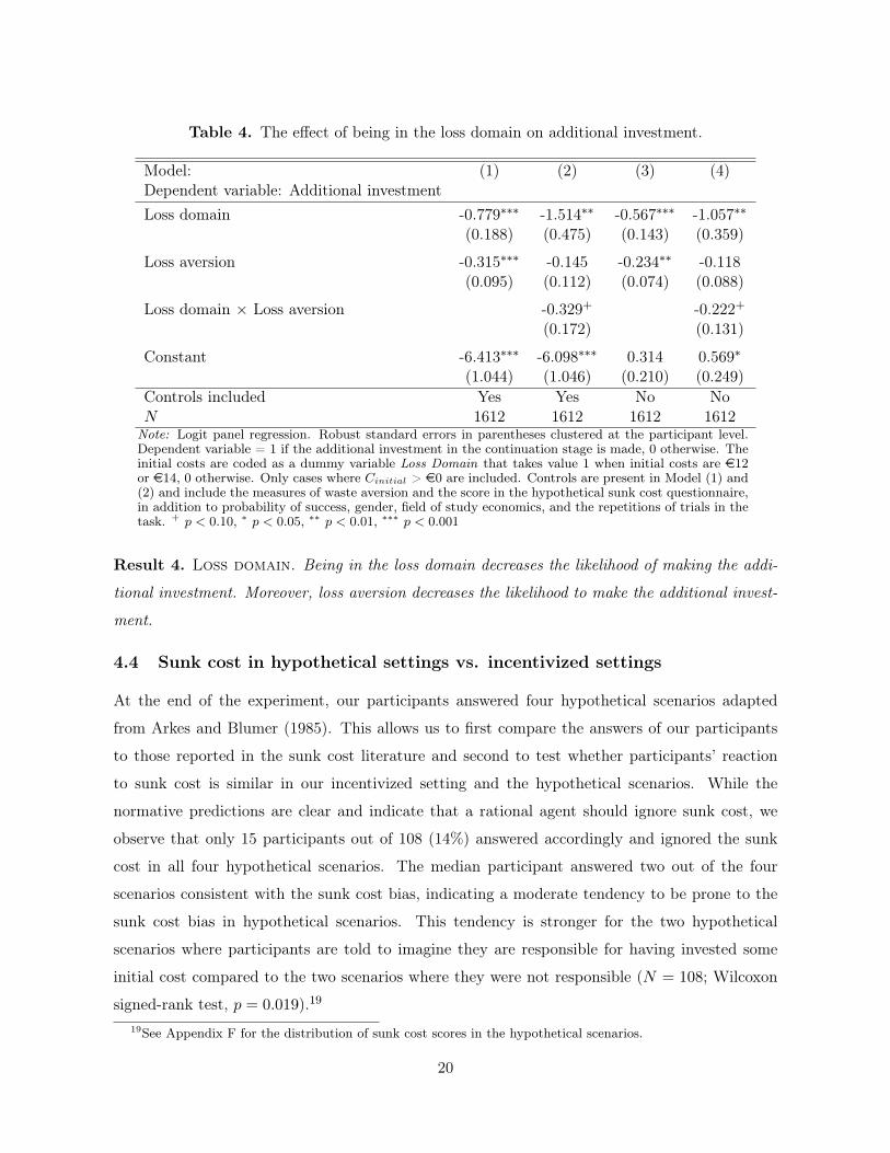
Table 4. The effect of being in the loss domain on additional investment.

Model: (1) (2) (3) (4)Dependent variable: Additional investmentLoss domain -0.779∗∗∗ -1.514∗∗ -0.567∗∗∗ -1.057∗∗

(0.188) (0.475) (0.143) (0.359)

Loss aversion -0.315∗∗∗ -0.145 -0.234∗∗ -0.118(0.095) (0.112) (0.074) (0.088)

Loss domain × Loss aversion -0.329+ -0.222+

(0.172) (0.131)

Constant -6.413∗∗∗ -6.098∗∗∗ 0.314 0.569∗

(1.044) (1.046) (0.210) (0.249)Controls included Yes Yes No NoN 1612 1612 1612 1612

Note: Logit panel regression. Robust standard errors in parentheses clustered at the participant level.Dependent variable = 1 if the additional investment in the continuation stage is made, 0 otherwise. Theinitial costs are coded as a dummy variable Loss Domain that takes value 1 when initial costs are e12or e14, 0 otherwise. Only cases where Cinitial > e0 are included. Controls are present in Model (1) and(2) and include the measures of waste aversion and the score in the hypothetical sunk cost questionnaire,in addition to probability of success, gender, field of study economics, and the repetitions of trials in thetask. + p < 0.10, ∗ p < 0.05, ∗∗ p < 0.01, ∗∗∗ p < 0.001

Result 4. Loss domain. Being in the loss domain decreases the likelihood of making the addi-

tional investment. Moreover, loss aversion decreases the likelihood to make the additional invest-

ment.

4.4 Sunk cost in hypothetical settings vs. incentivized settings

At the end of the experiment, our participants answered four hypothetical scenarios adapted

from Arkes and Blumer (1985). This allows us to first compare the answers of our participants

to those reported in the sunk cost literature and second to test whether participants’ reaction

to sunk cost is similar in our incentivized setting and the hypothetical scenarios. While the

normative predictions are clear and indicate that a rational agent should ignore sunk cost, we

observe that only 15 participants out of 108 (14%) answered accordingly and ignored the sunk

cost in all four hypothetical scenarios. The median participant answered two out of the four

scenarios consistent with the sunk cost bias, indicating a moderate tendency to be prone to the

sunk cost bias in hypothetical scenarios. This tendency is stronger for the two hypothetical

scenarios where participants are told to imagine they are responsible for having invested some

initial cost compared to the two scenarios where they were not responsible (N = 108; Wilcoxon

signed-rank test, p = 0.019).19

19See Appendix F for the distribution of sunk cost scores in the hypothetical scenarios.

20

Thus, our results in the hypothetical scenarios are generally in line with the findings reported

in Arkes and Blumer (1985) and we replicate them using a larger sample size. In addition, in our

within-subject design in the hypothetical scenarios, we also find support for the responsibility

effect as participants show a stronger tendency to show a sunk cost bias in the scenarios where

they were told to imagine to be responsible for the sunk cost compared to when they were asked

to imagined not to be responsible.

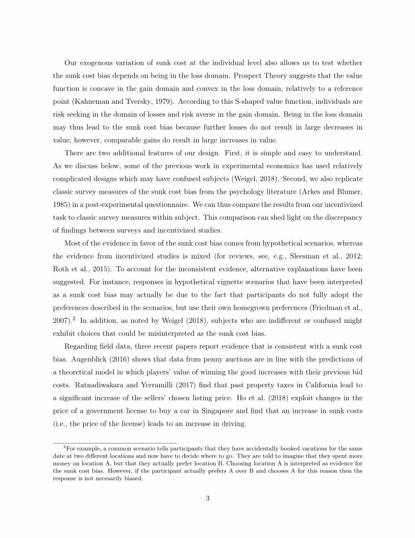
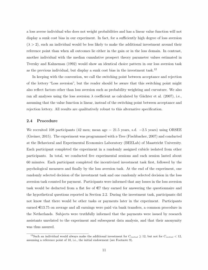
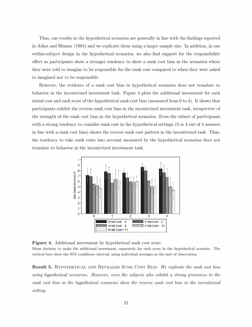
However, the evidence of a sunk cost bias in hypothetical scenarios does not translate to

behavior in the incentivized investment task. Figure 4 plots the additional investment for each

initial cost and each score of the hypothetical sunk cost bias (measured from 0 to 4). It shows that

participants exhibit the reverse sunk cost bias in the incentivized investment task, irrespective of

the strength of the sunk cost bias in the hypothetical scenarios. Even the subset of participants

with a strong tendency to consider sunk cost in the hypothetical settings (3 or 4 out of 4 answers

in line with a sunk cost bias) shows the reverse sunk cost pattern in the incentivized task. Thus,

the tendency to take sunk costs into account measured by the hypothetical scenarios does not

translate to behavior in the incentivized investment task.

Figure 4. Additional investment by hypothetical sunk cost score.Mean decision to make the additional investment, separately for each score in the hypothetical scenario. Thevertical bars show the 95% confidence interval, using individual averages as the unit of observation.

Result 5. Hypothetical and Revealed Sunk Cost Bias. We replicate the sunk cost bias

using hypothetical scenarios. However, even the subjects who exhibit a strong proneness to the

sunk cost bias in the hypothetical scenarios show the reverse sunk cost bias in the incentivized

setting.

21

5 Discussion and conclusion

Using a novel experimental design, we study the sunk cost bias in an incentivized setting and

assess potential channels underlying such an effect. We find that participants do indeed react

to exogenous variations in sunk cost, but not in the direction predicted by the sunk cost bias.

Instead, our main finding is that participants are less likely to make an additional investment the

higher the sunk cost. Our data thus provide evidence for a reverse sunk cost bias.

The overall pattern of our behavioral findings regarding the effect of sunk cost can be ratio-

nalized in different ways. For example, a risk averse decision maker with a CRRA utility function

who thinks about the payoffs from the experiment in isolation (i.e., considers only the money

in the experiment in the utility function instead of her total wealth) would be increasingly less

likely to make the additional investment as sunk costs increase.

A loss averse decision maker with linear utility in the loss and gain domain could also display a

behavioral pattern resembling the one we observe. This would be the case if the decision maker’s

reference point is somewhat lower than the endowment of e10. Such a reference point may reflect

the amount a participant expects to (minimally) gain for the time spent on the investment task.

For instance, with a reference point of e7 making the additional investment becomes a mixed

gamble for initial costs of at least e8. Thus, a sufficiently loss averse decision maker would be

less likely to make the additional investment than when initial costs are e0 and e4.

Our findings are also reminiscent of ideas suggested in two previous papers in the psychology

literature. Heath (1995) argues that participants set a mental limit for their expenditures when

this is easily feasible. When an expenditure reaches the mental limit, they quit investing. In a

study with hypothetical incentives, Zeelenberg and Van Dijk (1997) find that behavioral sunk

costs increase risk averse instead of risk seeking behavior in a subsequent monetary gamble. The

authors argue that this is more likely to occur when a risk avoiding choice allows reaching an

aspiration level. In our setup, an aspiration level equal to earning a positive payoff in the task

could explain that participants are more willing to gamble when the “losing” outcome of the

additional investment is considered satisfactory (with low Cinitial), but not when the “losing”

outcome fails to satisfy the aspiration level (with high Cinitial). We note however, that one could

also argue in favor of the opposite. If costs have been high, people could be far off their aspiration

levels and therefore willing to gamble in order to reach it. Exploring which exact channel is at

work would be an interesting question for future research.

Our results clearly show that findings using hypothetical scenarios do not necessarily trans-

late into behavior with real monetary consequences. Our findings in the hypothetical scenarios

22

replicate the ones in the seminal work by Arkes and Blumer (1985). However, even when con-

sidering only the participants who exhibit a strong hypothetical sunk cost bias, we observe a

reverse sunk cost bias in the incentivized setting. We consider this as strong evidence that stated

preferences elicited with questionnaires and revealed preferences using incentivized methods differ

substantially, at least in the sunk cost domain.

In addition to the incentives themselves, a potential explanation for this discrepancy could

be that the descriptions of the decision environments in the vignette studies leave room for

interpretation. The participants might therefore interpret the incentives differently than the

researchers intend and in a way that actually makes reacting to sunk cost rational. Mcafee

et al. (2010) characterize a broad range of environments in which this may be the case. For

example, reputational concerns could play a role. Some decision makers might believe that

stopping investing and admitting that the project failed would ruin their reputation as effective

decision makers (Davis et al., 1997), especially when they are responsible for the initial investment.

Our results for the hypothetical scenarios are consistent with this explanation as participants are

more sunk cost prone in the responsibility condition. Other misconceptions of the incentives

described in the hypothetical scenarios are also plausible. In contrast to this, the incentives in

our investment task are clear at every stage. Participants also make their investment decisions

privately and reputational concerns are thus absent.

Studies with hypothetical decision situations have found that responsibility leads to a greater

sunk cost bias (Sleesman et al., 2012; Staw, 1976). In our incentivized setting, we do not find that

responsibility for the initial investment affects the propensity to make the additional investment.

In that respect, a potential caveat regarding our within-subject design could be that subjects

would like to appear consistent. However, this should then also hold for the hypothetical decision

situations where we replicate, also within-subject, the responsibility effect found in previous

hypothetical studies.

Our paper contributes to the literature on the sunk cost bias and our findings underline the

need for more controlled laboratory experiments with real consequences. For instance, one avenue

of future research could be to test whether a more vivid and engaging initial investment (e.g.,

real effort task) is a crucial component for the sunk cost bias to emerge. In addition, one could

also test the role of different proximity to project completion (Conlon and Garland, 1993) and

different accountability in terms of reputational loss (Fox and Staw, 1979). In any case, the search

for the sunk cost bias in the laboratory needs to go on.

23

References

Arkes and Ayton, P. (1999). The sunk cost and Concorde effects: Are humans less rational than

lower animals? Psychological Bulletin, 125(5):591–600.

Arkes and Blumer, C. (1985). The psychology of sunk cost. Organizational Behavior and Human

Decision, 35(1):124–140.

Ashraf, N., Berry, J., and Shapiro, J. M. (2010). Can higher prices stimulate product use?

Evidence from a field experiment in Zambia. American Economic Review, 100(5):2383–2413.

Augenblick, N. (2016). The Sunk-Cost Fallacy in Penny Auctions. The Review of Economic

Studies, 83(1):58–86.

Bazerman, M. H., Giuliano, T., and Appelman, A. (1984). Escalation of commitment in individual

and group decision making. Organizational Behavior and Human Performance, 33(2):141–152.

Bogdanov, M., Ruff, C. C., and Schwabe, L. (2017). Transcranial Stimulation Over the Dorso-

lateral Prefrontal Cortex Increases the Impact of Past Expenses on Decision-Making. Cerebral

Cortex, 27(2):1094–1102.

Brockner, J. (1992). The Escalation of Commitment to a Failing Course of Action: Toward

Theoretical Progress. Academy of Management Review, 17(1):39.

Cason, T. N. and Plott, C. R. (2014). Misconceptions and game form recognition: Challenges to

theories of revealed preference and framing. Journal of Political Economy, 122(6):1235–1270.

Conlon, D. E. and Garland, H. (1993). The Role of Project Completion Information in Resource

Allocation Decisions. Academy of Management Journal, 36(2):402–413.

Davis, J. H., Schoorman, F. D., and Donaldson, L. (1997). Toward a stewardship theory of

management. Academy of Management Review, 22(1):20–47.

Fischbacher, U. (2007). z-tree: Zurich toolbox for ready-made economic experiments. Experi-

mental Economics, 10(2):171–178.

Fox, F. V. and Staw, B. M. (1979). The Trapped Administrator: Effects of Job Insecurity and

Policy Resistance Upon Commitment to a Course of Action. Administrative Science Quarterly,

24(3):449.

Friedman, D., Pommerenke, K., Lukose, R., Milam, G., and Huberman, B. A. (2007). Searching

for the sunk cost fallacy. Experimental Economics, 10(1):79–104.

Gächter, S., Johnson, E., and Herrmann, A. (2007). Individual-level loss aversion in riskless and

risky choices. Institute for the Study of Labor (IZA), IZA Discussion Papers.

Greiner, B. (2015). Subject pool recruitment procedures: organizing experiments with ORSEE.

24

Journal of the Economic Science Association, 1(1):114–125.

Haita-Falah, C. (2017). Sunk-cost fallacy and cognitive ability in individual decision-making.

Journal of Economic Psychology, 58:44–59.

Haller, A. and Schwabe, L. (2014). Sunk costs in the human brain. Neuroimage, 97:127–133.

Heath, C. (1995). Escalation and De-escalation of Commitment in Response to Sunk Costs:

The Role of Budgeting in Mental Accounting. Organizational Behavior and Human Decision

Processes, 62(1):38–54.

Ho, T. H., Png, I. P., and Reza, S. (2018). Sunk cost fallacy in driving the world’s costliest cars.

Management Science, 64(4):1761–1778.

Holt, C. A. and Laury, S. K. (2002). Risk aversion and incentive effects. American Economic

Review, 92(5):1644–1655.

Kahneman, D. and Tversky, A. (1979). Prospect Theory: An Analysis of Decision under Risk.

Econometrica, 47(2):263.

Ketel, N., Linde, J., Oosterbeek, H., and van der Klaauw, B. (2016). Tuition Fees and Sunk-cost

Effects. The Economic Journal, 126(598):2342–2362.

Kirby, S. L. and Davis, M. A. (1998). A study of escalating commitment in principal-agent

relationships: Effects of monitoring and personal responsibility. Journal of Applied Psychology,

83(2):206–217.

Mcafee, R. P., Mialon, H. M., and Mialon, S. H. (2010). Do sunk costs matter? Economic

Inquiry, 48(2):323–336.

Molden, D. C. and Hui, C. M. (2011). Promoting de-escalation of commitment: A regulatory-

focus perspective on sunk costs. Psychological Science, 22(1):8–12.

Offerman, T. and Potters, J. (2006). Does auctioning of entry licences induce collusion? an

experimental study. The Review of Economic Studies, 73(3):769–791.

Phillips, O. R., Battalio, R. C., and Kogut, C. A. (1991). Sunk and Opportunity Costs in

Valuation and Bidding. Southern Economic Journal, 58(1):112.

Ratnadiwakara, D. and Yerramilli, V. (2017). Sunk-cost fallacy and seller behavior in the housing

market. Working paper. Available at SSRN: https://ssrn.com/abstract=3040712.

Ronayne, D., Sgroi, D., and Tuckwell, A. (2020). Evaluating the sunk cost effect. Working paper.

Competitive Advantage in the Global Economy (CAGE) No. 475.

Ross, J. and Staw, B. M. (1993). Organizational escalation and exit: Lessons from the shoreham

nuclear power plant. Academy of Management journal, 36(4):701–732.

Roth, S., Robbert, T., and Straus, L. (2015). On the sunk-cost effect in economic decision-making:

25

a meta-analytic review. Business Research, 8(1):99–138.

Schoorman, F. D. and Holahan, P. J. (1996). Psychological antecedents of escalation behavior:

Effects of choice, responsibility, and decision consequences. Journal of Applied Psychology,

81(6):786.

Schulz, A. K. and Cheng, M. M. (2002). Persistence in capital budgeting reinvestment decisions -

Personal responsibility antecedent and information asymmetry moderator: A note. Accounting

and Finance, 42(1):73–86.

Sleesman, D. J., Conlon, D. E., McNamara, G., and Miles, J. E. (2012). Cleaning up the big

muddy: A meta-analytic review of the determinants of escalation of commitment. Academy of

Management Journal, 55(3):541–562.

Sokol-Hessner, P., Hsu, M., Curley, N. G., Delgado, M. R., Camerer, C. F., and Phelps, E. A.

(2009). Thinking like a trader selectively reduces individuals’ loss aversion. Proceedings of the

National Academy of Sciences, 106(13):5035–5040.

Soman, D. and Cheema, A. (2001). The Effect of Windfall Gains on the Sunk-Cost Effect.

Marketing Letters, 12(1):51–62.

Staw, B. M. (1976). Knee-deep in the big muddy: a study of escalating commitment to a chosen

course of action. Organizational Behavior and Human Performance, 16(1):27–44.

Strough, J. N., Mehta, C. M., McFall, J. P., and Schuller, K. L. (2008). Are older adults less

subject to the sunk-cost fallacy than younger adults?: Short report. Psychological Science,

19(7):650–652.

Strube, M. J. (1988). The decision to leave an abusive relationship: Empirical evidence and

theoretical issues. Psychological Bulletin, 104(2):236–250.

Tversky, A. and Kahneman, D. (1992). Advances in prospect theory: Cumulative representation

of uncertainty. Journal of Risk and Uncertainty, 5(4):297–323.

Weigel, C. (2018). Don’t stop now: The sunk cost effect in an incentivized lab experiment.

Working Paper. Available at SSRN: https://ssrn.com/abstract=3207806.

Zeelenberg, M. and Van Dijk, E. (1997). A reverse sunk cost effect in risky decision making:

Sometimes we have too much invested to gamble. Journal of Economic Psychology, 18(6):677–

691.

26

Appendix

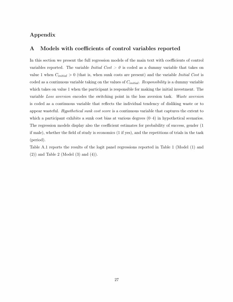
A Models with coefficients of control variables reported

In this section we present the full regression models of the main text with coefficients of control

variables reported. The variable Initial Cost > 0 is coded as a dummy variable that takes on

value 1 when Cinitial > 0 (that is, when sunk costs are present) and the variable Initial Cost is

coded as a continuous variable taking on the values of Cinitial. Responsibility is a dummy variable

which takes on value 1 when the participant is responsible for making the initial investment. The

variable Loss aversion encodes the switching point in the loss aversion task. Waste aversion

is coded as a continuous variable that reflects the individual tendency of disliking waste or to

appear wasteful. Hypothetical sunk cost score is a continuous variable that captures the extent to

which a participant exhibits a sunk cost bias at various degrees (0–4) in hypothetical scenarios.

The regression models display also the coefficient estimates for probability of success, gender (1

if male), whether the field of study is economics (1 if yes), and the repetitions of trials in the task

(period).

Table A.1 reports the results of the logit panel regressions reported in Table 1 (Model (1) and

(2)) and Table 2 (Model (3) and (4)).

27

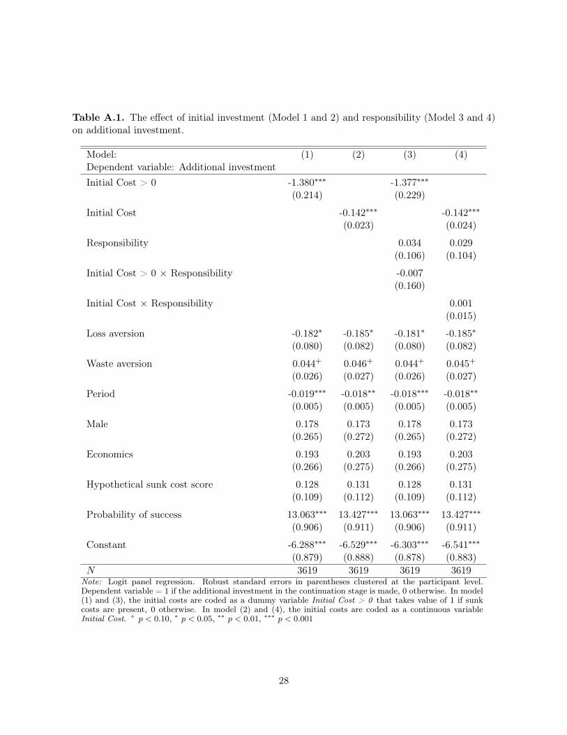
Table A.1. The effect of initial investment (Model 1 and 2) and responsibility (Model 3 and 4)on additional investment.

Model: (1) (2) (3) (4)Dependent variable: Additional investmentInitial Cost > 0 -1.380∗∗∗ -1.377∗∗∗

(0.214) (0.229)

Initial Cost -0.142∗∗∗ -0.142∗∗∗

(0.023) (0.024)

Responsibility 0.034 0.029(0.106) (0.104)

Initial Cost > 0 × Responsibility -0.007(0.160)

Initial Cost × Responsibility 0.001(0.015)

Loss aversion -0.182∗ -0.185∗ -0.181∗ -0.185∗

(0.080) (0.082) (0.080) (0.082)

Waste aversion 0.044+ 0.046+ 0.044+ 0.045+

(0.026) (0.027) (0.026) (0.027)

Period -0.019∗∗∗ -0.018∗∗ -0.018∗∗∗ -0.018∗∗

(0.005) (0.005) (0.005) (0.005)

Male 0.178 0.173 0.178 0.173(0.265) (0.272) (0.265) (0.272)

Economics 0.193 0.203 0.193 0.203(0.266) (0.275) (0.266) (0.275)

Hypothetical sunk cost score 0.128 0.131 0.128 0.131(0.109) (0.112) (0.109) (0.112)

Probability of success 13.063∗∗∗ 13.427∗∗∗ 13.063∗∗∗ 13.427∗∗∗

(0.906) (0.911) (0.906) (0.911)

Constant -6.288∗∗∗ -6.529∗∗∗ -6.303∗∗∗ -6.541∗∗∗

(0.879) (0.888) (0.878) (0.883)N 3619 3619 3619 3619

Note: Logit panel regression. Robust standard errors in parentheses clustered at the participant level.Dependent variable = 1 if the additional investment in the continuation stage is made, 0 otherwise. In model(1) and (3), the initial costs are coded as a dummy variable Initial Cost > 0 that takes value of 1 if sunkcosts are present, 0 otherwise. In model (2) and (4), the initial costs are coded as a continuous variableInitial Cost. + p < 0.10, ∗ p < 0.05, ∗∗ p < 0.01, ∗∗∗ p < 0.001

28

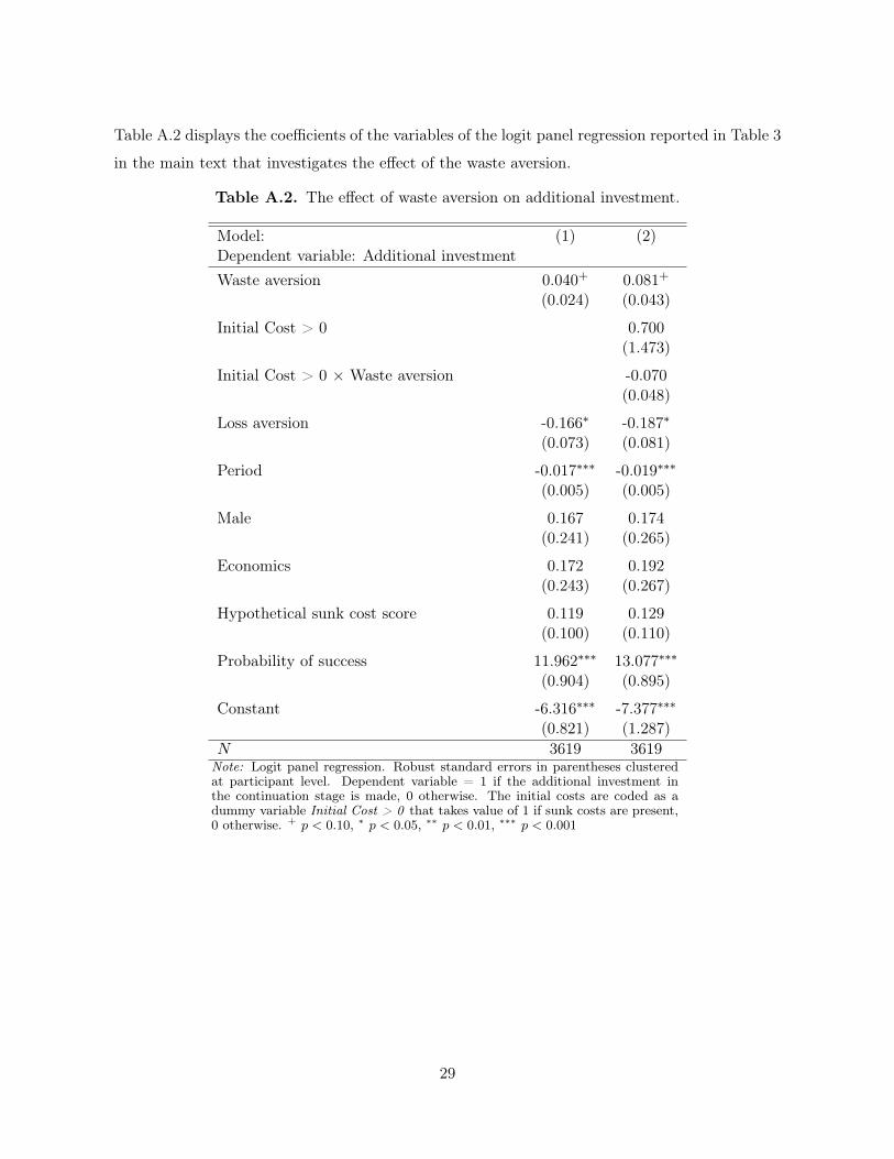
Table A.2 displays the coefficients of the variables of the logit panel regression reported in Table 3

in the main text that investigates the effect of the waste aversion.

Table A.2. The effect of waste aversion on additional investment.

Model: (1) (2)Dependent variable: Additional investmentWaste aversion 0.040+ 0.081+

(0.024) (0.043)

Initial Cost > 0 0.700(1.473)

Initial Cost > 0 × Waste aversion -0.070(0.048)

Loss aversion -0.166∗ -0.187∗

(0.073) (0.081)

Period -0.017∗∗∗ -0.019∗∗∗

(0.005) (0.005)

Male 0.167 0.174(0.241) (0.265)

Economics 0.172 0.192(0.243) (0.267)

Hypothetical sunk cost score 0.119 0.129(0.100) (0.110)

Probability of success 11.962∗∗∗ 13.077∗∗∗

(0.904) (0.895)

Constant -6.316∗∗∗ -7.377∗∗∗

(0.821) (1.287)N 3619 3619

Note: Logit panel regression. Robust standard errors in parentheses clusteredat participant level. Dependent variable = 1 if the additional investment inthe continuation stage is made, 0 otherwise. The initial costs are coded as adummy variable Initial Cost > 0 that takes value of 1 if sunk costs are present,0 otherwise. + p < 0.10, ∗ p < 0.05, ∗∗ p < 0.01, ∗∗∗ p < 0.001

29

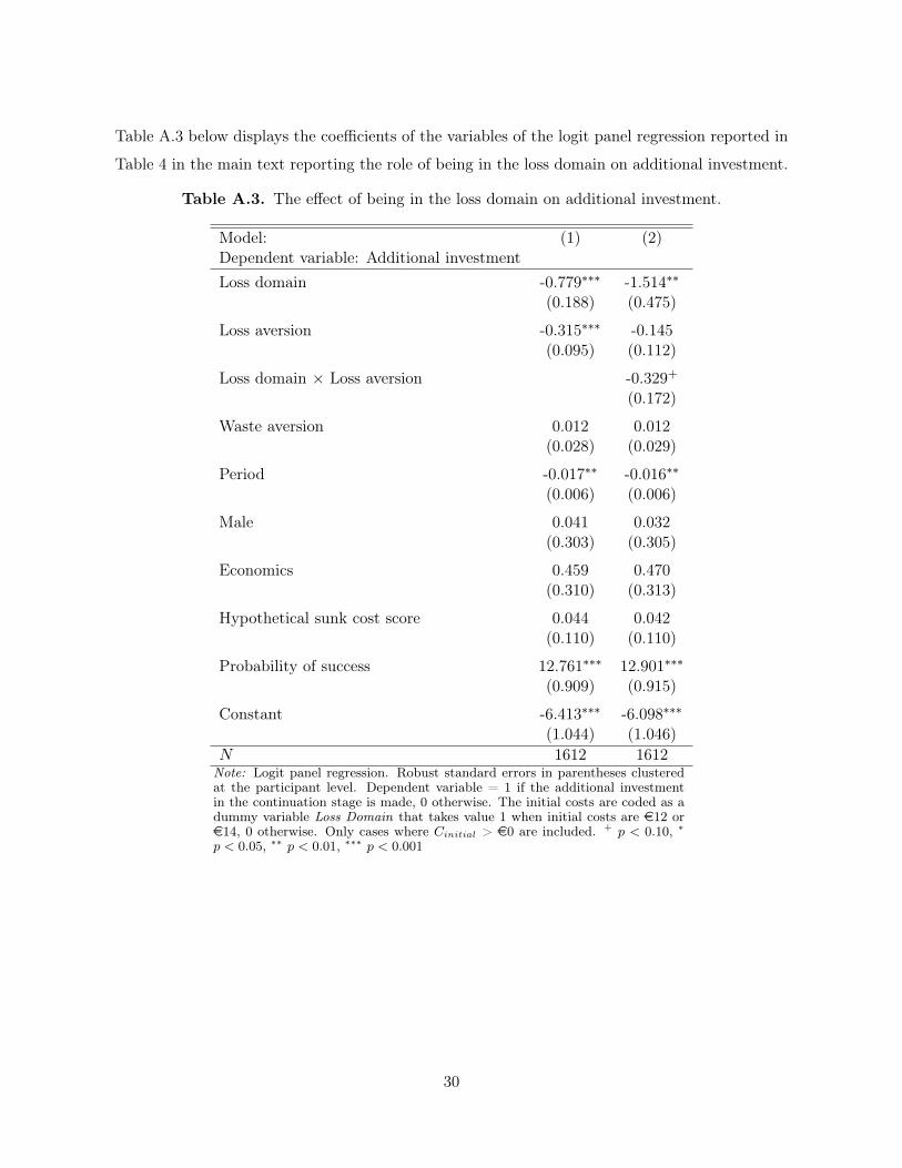
Table A.3 below displays the coefficients of the variables of the logit panel regression reported in

Table 4 in the main text reporting the role of being in the loss domain on additional investment.

Table A.3. The effect of being in the loss domain on additional investment.

Model: (1) (2)Dependent variable: Additional investmentLoss domain -0.779∗∗∗ -1.514∗∗

(0.188) (0.475)

Loss aversion -0.315∗∗∗ -0.145(0.095) (0.112)

Loss domain × Loss aversion -0.329+

(0.172)

Waste aversion 0.012 0.012(0.028) (0.029)

Period -0.017∗∗ -0.016∗∗

(0.006) (0.006)

Male 0.041 0.032(0.303) (0.305)

Economics 0.459 0.470(0.310) (0.313)

Hypothetical sunk cost score 0.044 0.042(0.110) (0.110)

Probability of success 12.761∗∗∗ 12.901∗∗∗

(0.909) (0.915)

Constant -6.413∗∗∗ -6.098∗∗∗

(1.044) (1.046)N 1612 1612

Note: Logit panel regression. Robust standard errors in parentheses clusteredat the participant level. Dependent variable = 1 if the additional investmentin the continuation stage is made, 0 otherwise. The initial costs are coded as adummy variable Loss Domain that takes value 1 when initial costs are e12 ore14, 0 otherwise. Only cases where Cinitial > e0 are included. + p < 0.10, ∗

p < 0.05, ∗∗ p < 0.01, ∗∗∗ p < 0.001

30

B Robustness checks

In this section we present different robustness checks of the regression model investigating the

role of the initial investment and the role of responsibility (Hypothesis 1 and Hypothesis 2). The

main finding of a reverse sunk cost effect and the null effect of responsibility are robust and

present in all the different checks reported below, such as when considering only the participants

who always made the initial investment when responsible for it, when analyzing only those who

not always make the initial investment when responsible for it, or when using a linear probability

model instead of a logit model.

B.1 Only participants who always made the initial investment

Table B.1 includes only those participants who always made the initial investment when respon-

sible for it. Model (1) and (2) reports the effect of the initial investment on the likelihood to

make the additional investment (cf. Table 1 in the main text). Model (3) and (4) report the

effect of responsibility (cf. Table 2 in the main text).

31

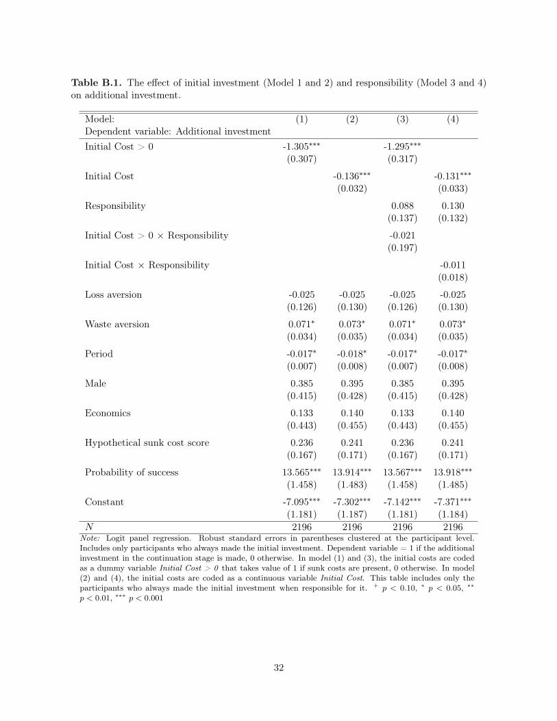
Table B.1. The effect of initial investment (Model 1 and 2) and responsibility (Model 3 and 4)on additional investment.

Model: (1) (2) (3) (4)Dependent variable: Additional investmentInitial Cost > 0 -1.305∗∗∗ -1.295∗∗∗

(0.307) (0.317)

Initial Cost -0.136∗∗∗ -0.131∗∗∗

(0.032) (0.033)

Responsibility 0.088 0.130(0.137) (0.132)

Initial Cost > 0 × Responsibility -0.021(0.197)

Initial Cost × Responsibility -0.011(0.018)

Loss aversion -0.025 -0.025 -0.025 -0.025(0.126) (0.130) (0.126) (0.130)

Waste aversion 0.071∗ 0.073∗ 0.071∗ 0.073∗

(0.034) (0.035) (0.034) (0.035)

Period -0.017∗ -0.018∗ -0.017∗ -0.017∗

(0.007) (0.008) (0.007) (0.008)

Male 0.385 0.395 0.385 0.395(0.415) (0.428) (0.415) (0.428)

Economics 0.133 0.140 0.133 0.140(0.443) (0.455) (0.443) (0.455)

Hypothetical sunk cost score 0.236 0.241 0.236 0.241(0.167) (0.171) (0.167) (0.171)

Probability of success 13.565∗∗∗ 13.914∗∗∗ 13.567∗∗∗ 13.918∗∗∗

(1.458) (1.483) (1.458) (1.485)

Constant -7.095∗∗∗ -7.302∗∗∗ -7.142∗∗∗ -7.371∗∗∗

(1.181) (1.187) (1.181) (1.184)N 2196 2196 2196 2196

Note: Logit panel regression. Robust standard errors in parentheses clustered at the participant level.Includes only participants who always made the initial investment. Dependent variable = 1 if the additionalinvestment in the continuation stage is made, 0 otherwise. In model (1) and (3), the initial costs are codedas a dummy variable Initial Cost > 0 that takes value of 1 if sunk costs are present, 0 otherwise. In model(2) and (4), the initial costs are coded as a continuous variable Initial Cost. This table includes only theparticipants who always made the initial investment when responsible for it. + p < 0.10, ∗ p < 0.05, ∗∗

p < 0.01, ∗∗∗ p < 0.001

32

B.2 Only participants who did not always make the initial investment

Table B.2 below includes only those participants who did not always made the initial investment

when responsible for it. Model (1) and (2) reports the effect of the initial investment on the

likelihood of making the additional investment (cf. Table 1 in the main text). Model (3) and (4)

reports the effect of responsibility of the initial investment (cf. Table 2 in the main text).

33

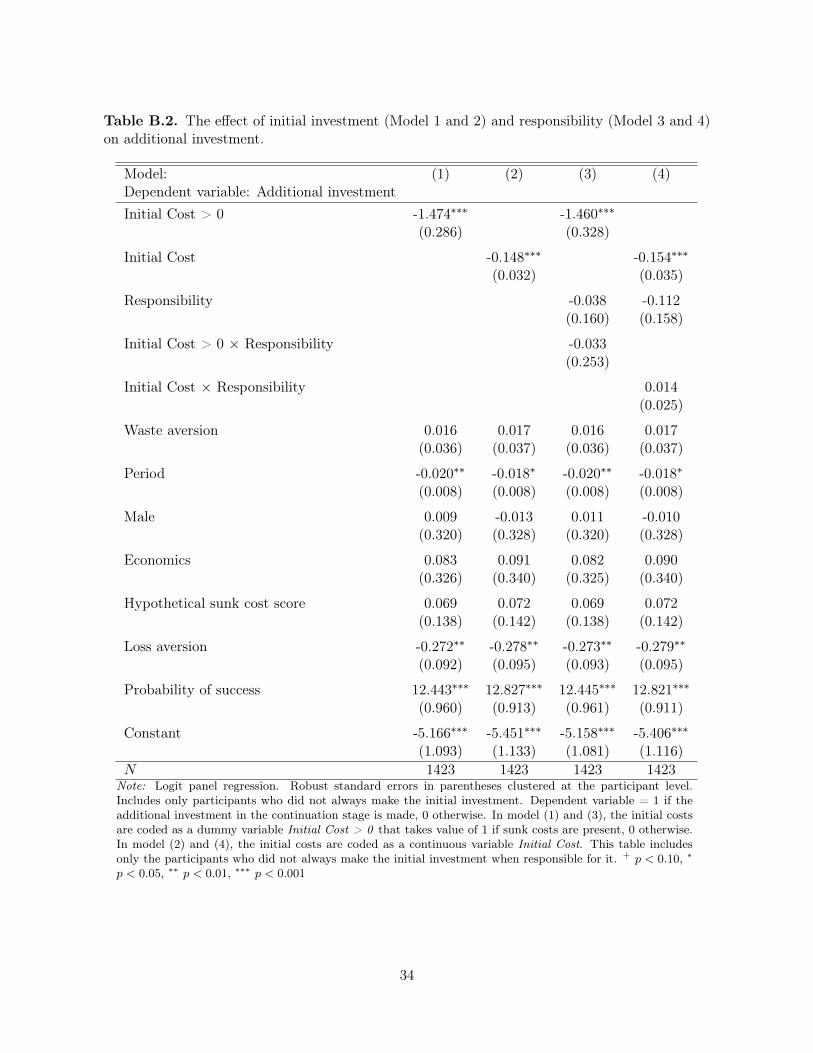
Table B.2. The effect of initial investment (Model 1 and 2) and responsibility (Model 3 and 4)on additional investment.

Model: (1) (2) (3) (4)Dependent variable: Additional investmentInitial Cost > 0 -1.474∗∗∗ -1.460∗∗∗

(0.286) (0.328)

Initial Cost -0.148∗∗∗ -0.154∗∗∗

(0.032) (0.035)

Responsibility -0.038 -0.112(0.160) (0.158)

Initial Cost > 0 × Responsibility -0.033(0.253)

Initial Cost × Responsibility 0.014(0.025)

Waste aversion 0.016 0.017 0.016 0.017(0.036) (0.037) (0.036) (0.037)

Period -0.020∗∗ -0.018∗ -0.020∗∗ -0.018∗

(0.008) (0.008) (0.008) (0.008)

Male 0.009 -0.013 0.011 -0.010(0.320) (0.328) (0.320) (0.328)

Economics 0.083 0.091 0.082 0.090(0.326) (0.340) (0.325) (0.340)

Hypothetical sunk cost score 0.069 0.072 0.069 0.072(0.138) (0.142) (0.138) (0.142)

Loss aversion -0.272∗∗ -0.278∗∗ -0.273∗∗ -0.279∗∗

(0.092) (0.095) (0.093) (0.095)

Probability of success 12.443∗∗∗ 12.827∗∗∗ 12.445∗∗∗ 12.821∗∗∗

(0.960) (0.913) (0.961) (0.911)

Constant -5.166∗∗∗ -5.451∗∗∗ -5.158∗∗∗ -5.406∗∗∗

(1.093) (1.133) (1.081) (1.116)N 1423 1423 1423 1423

Note: Logit panel regression. Robust standard errors in parentheses clustered at the participant level.Includes only participants who did not always make the initial investment. Dependent variable = 1 if theadditional investment in the continuation stage is made, 0 otherwise. In model (1) and (3), the initial costsare coded as a dummy variable Initial Cost > 0 that takes value of 1 if sunk costs are present, 0 otherwise.In model (2) and (4), the initial costs are coded as a continuous variable Initial Cost. This table includesonly the participants who did not always make the initial investment when responsible for it. + p < 0.10, ∗

p < 0.05, ∗∗ p < 0.01, ∗∗∗ p < 0.001

34

B.3 Linear probability models instead of logit regression models

Table B.3 presents regression results using a linear probability model instead of a logit model.

Model (1) and (2) reports the effect of the initial investment on the likelihood of making the

additional investment (cf. Table 1 in the main text). Model (3) and (4) reports the effect of

responsibility of the initial investment (cf. Table 2 in the main text).

35

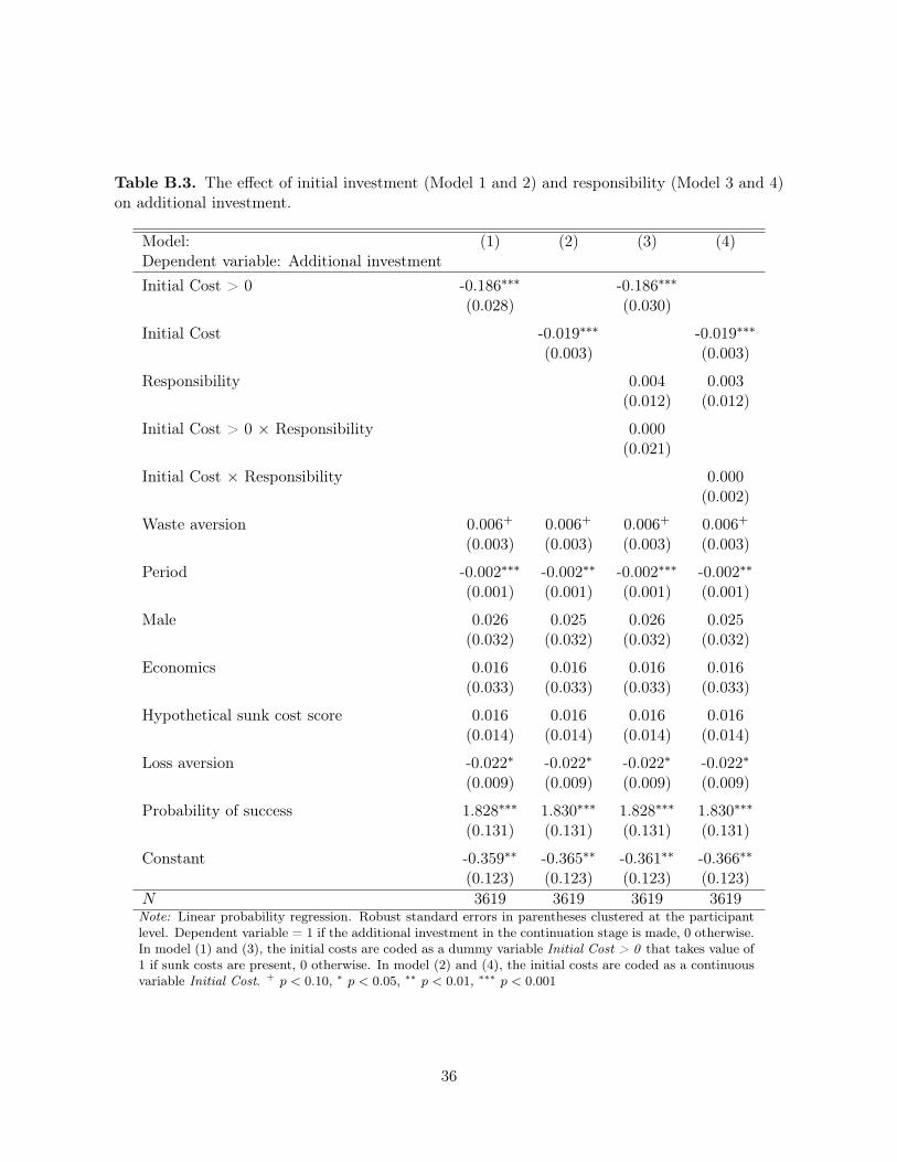
Table B.3. The effect of initial investment (Model 1 and 2) and responsibility (Model 3 and 4)on additional investment.

Model: (1) (2) (3) (4)Dependent variable: Additional investmentInitial Cost > 0 -0.186∗∗∗ -0.186∗∗∗

(0.028) (0.030)

Initial Cost -0.019∗∗∗ -0.019∗∗∗

(0.003) (0.003)

Responsibility 0.004 0.003(0.012) (0.012)

Initial Cost > 0 × Responsibility 0.000(0.021)

Initial Cost × Responsibility 0.000(0.002)

Waste aversion 0.006+ 0.006+ 0.006+ 0.006+

(0.003) (0.003) (0.003) (0.003)

Period -0.002∗∗∗ -0.002∗∗ -0.002∗∗∗ -0.002∗∗

(0.001) (0.001) (0.001) (0.001)

Male 0.026 0.025 0.026 0.025(0.032) (0.032) (0.032) (0.032)

Economics 0.016 0.016 0.016 0.016(0.033) (0.033) (0.033) (0.033)

Hypothetical sunk cost score 0.016 0.016 0.016 0.016(0.014) (0.014) (0.014) (0.014)

Loss aversion -0.022∗ -0.022∗ -0.022∗ -0.022∗

(0.009) (0.009) (0.009) (0.009)

Probability of success 1.828∗∗∗ 1.830∗∗∗ 1.828∗∗∗ 1.830∗∗∗

(0.131) (0.131) (0.131) (0.131)

Constant -0.359∗∗ -0.365∗∗ -0.361∗∗ -0.366∗∗

(0.123) (0.123) (0.123) (0.123)N 3619 3619 3619 3619Note: Linear probability regression. Robust standard errors in parentheses clustered at the participantlevel. Dependent variable = 1 if the additional investment in the continuation stage is made, 0 otherwise.In model (1) and (3), the initial costs are coded as a dummy variable Initial Cost > 0 that takes value of1 if sunk costs are present, 0 otherwise. In model (2) and (4), the initial costs are coded as a continuousvariable Initial Cost. + p < 0.10, ∗ p < 0.05, ∗∗ p < 0.01, ∗∗∗ p < 0.001

36

C Initial cost as dummy variables

Table C.1 shows the results of a logit panel regression testing for the effect of each initial cost

on the additional investment. Each initial cost is coded as a dummy variable. The results of the

comparison between levels is summarized below.

• All the estimated coefficients for each initial cost level are negative and significantly different

from Initial cost = 0 (p < 0.001).

• Initial cost = 4 is significantly different from all the other Initial cost level (p < 0.001).

• Initial cost = 8 is not significantly different from Initial cost = 12 (p = 0.122) and from

Initial cost = 14 (p = 0.018).

• Initial cost = 12 is not significantly different from Initial cost = 14 (p = 0.405).

37

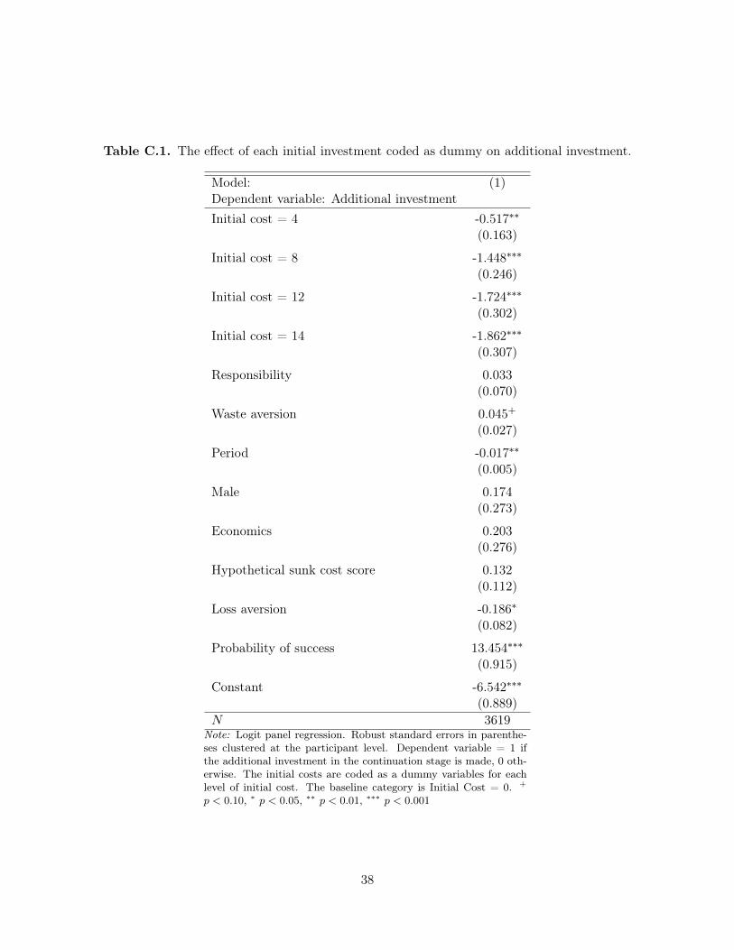
Table C.1. The effect of each initial investment coded as dummy on additional investment.

Model: (1)Dependent variable: Additional investmentInitial cost = 4 -0.517∗∗

(0.163)

Initial cost = 8 -1.448∗∗∗

(0.246)

Initial cost = 12 -1.724∗∗∗

(0.302)

Initial cost = 14 -1.862∗∗∗

(0.307)

Responsibility 0.033(0.070)

Waste aversion 0.045+

(0.027)

Period -0.017∗∗

(0.005)

Male 0.174(0.273)

Economics 0.203(0.276)

Hypothetical sunk cost score 0.132(0.112)

Loss aversion -0.186∗

(0.082)

Probability of success 13.454∗∗∗

(0.915)

Constant -6.542∗∗∗

(0.889)N 3619

Note: Logit panel regression. Robust standard errors in parenthe-ses clustered at the participant level. Dependent variable = 1 ifthe additional investment in the continuation stage is made, 0 oth-erwise. The initial costs are coded as a dummy variables for eachlevel of initial cost. The baseline category is Initial Cost = 0. +

p < 0.10, ∗ p < 0.05, ∗∗ p < 0.01, ∗∗∗ p < 0.001

38

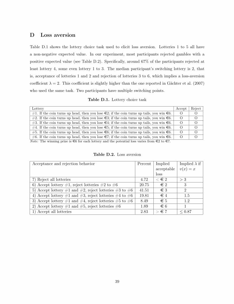
D Loss aversion

Table D.1 shows the lottery choice task used to elicit loss aversion. Lotteries 1 to 5 all have

a non-negative expected value. In our experiment, most participants rejected gambles with a

positive expected value (see Table D.2). Specifically, around 67% of the participants rejected at

least lottery 4, some even lottery 1 to 3. The median participant’s switching lottery is 2, that

is, acceptance of lotteries 1 and 2 and rejection of lotteries 3 to 6, which implies a loss-aversion

coefficient λ = 2. This coefficient is slightly higher than the one reported in Gächter et al. (2007)

who used the same task. Two participants have multiple switching points.

Table D.1. Lottery choice task

Lottery Accept Reject#1. If the coin turns up head, then you lose e2; if the coin turns up tails, you win e6. O O#2. If the coin turns up head, then you lose e3; if the coin turns up tails, you win e6. O O#3. If the coin turns up head, then you lose e4; if the coin turns up tails, you win e6. O O#4. If the coin turns up head, then you lose e5; if the coin turns up tails, you win e6. O O#5. If the coin turns up head, then you lose e6; if the coin turns up tails, you win e6. O O#6. If the coin turns up head, then you lose e7; if the coin turns up tails, you win e6. O O

Note: The winning prize is e6 for each lottery and the potential loss varies from e2 to e7.

Table D.2. Loss aversion

Acceptance and rejection behavior Percent Impliedacceptableloss

Implied λ ifv(x) = x

7) Reject all lotteries 4.72 < e 2 > 3

6) Accept lottery #1, reject lotteries #2 to #6 20.75 e 2 35) Accept lottery #1 and #2, reject lotteries #3 to #6 41.51 e 3 24) Accept lottery #1 and #3, reject lotteries #4 to #6 19.81 e 4 1.53) Accept lottery #1 and #4, reject lotteries #5 to #6 8.49 e 5 1.22) Accept lottery #1 and #5, reject lotteries #6 1.89 e 6 11) Accept all lotteries 2.83 > e 7 ≤ 0.87

39

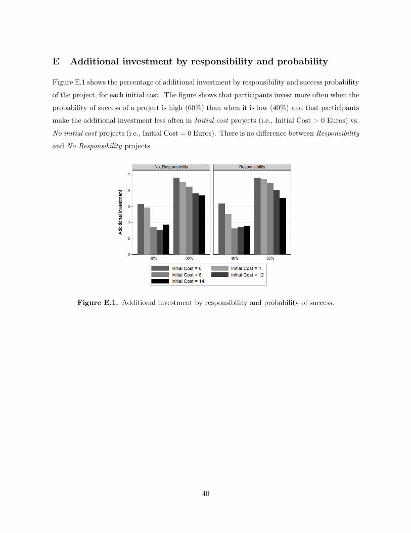
E Additional investment by responsibility and probability

Figure E.1 shows the percentage of additional investment by responsibility and success probability

of the project, for each initial cost. The figure shows that participants invest more often when the

probability of success of a project is high (60%) than when it is low (40%) and that participants

make the additional investment less often in Initial cost projects (i.e., Initial Cost > 0 Euros) vs.

No initial cost projects (i.e., Initial Cost = 0 Euros). There is no difference between Responsibility

and No Responsibility projects.

Figure E.1. Additional investment by responsibility and probability of success.

40

F Hypothetical sunk cost score

Below are the hypothetical scenarios used in the sunk cost questionnaire. We adapted vignettes

1, 3A, 8 and 9 used in Arkes and Blumer (1985). Textual changes to the original versions are

emphasized in italic. The original text is shown between brackets.

1. Responsibility. Imagine that you have spent e400 [$100] on a ticket for a weekend ski trip

to France [Michigan]. Several weeks later you buy a e200 [$50] ticket for a weekend ski trip to

Italy [Wisconsin]. You think you will enjoy the Italy [Wisconsin] ski trip more than the France

[Michigan] ski trip. As you are putting your just-purchased Italy [Wisconsin] ski trip ticket in

your wallet, you notice that the France [Michigan] ski trip and the Italy [Wisconsin] ski trip are

for the same weekend! It’s too late to sell either ticket, and you cannot return either one. You

must use one ticket and not the other. Which ski trip will you go on?

Sunk cost answers: France (45/108 participants, 41.67%; in Arkes and Blumer (1985): 64%)

2. Responsibility. As the president of an airline company, you have invested 10 million Euros

[dollars] of the company’s money into a research project. The purpose was to build a plane that

would not be detected by conventional radar, in other words, a radar-blank plane. When the

project is 90% completed, another firm begins marketing a plane that cannot be detected by

radar. Also, it is apparent that their plane is much faster and far more economical than the plane

your company is building. The question is: should you invest the last 10% of the research funds

to finish your radar-blank plane?

Sunk cost answer: Yes (74/108 participants, 68.52%; in Arkes and Blumer (1985): 85%)

3. No Responsibility. The Acme Airline Company has invested 10 million Euros [dollars] of the

company’s money into a research project. The purpose was to build a plane that would not be

detected by conventional radar, in other words, a radar-blank plane. When the project is 90%

completed, another firm begins marketing a plane that cannot be detected by radar. Also, it is

apparent that their plane is much faster and more economical than the plane Acme is building.

The question is should Acme Airlines invest the last million Euros of its research funds to finish

the radar-blank plane?

Sunk cost answer: Yes (74/108 participants, 68.52%; in Arkes and Blumer (1985): 63%)

4. No Responsibility. As you are listening to the radio one morning, the disk jockey calls you.

He informs you that you have won a free ski trip to either France [Michigan] or Italy [Wisconsin]

41

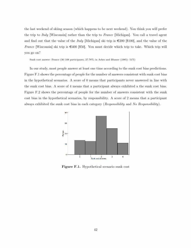
the last weekend of skiing season (which happens to be next weekend). You think you will prefer

the trip to Italy [Wisconsin] rather than the trip to France [Michigan]. You call a travel agent

and find out that the value of the Italy [Michigan] ski trip is e200 [$100], and the value of the

France [Wisconsin] ski trip is e400 [$50]. You must decide which trip to take. Which trip will

you go on?

Sunk cost answer: France (30/108 participants, 27.78%; in Arkes and Blumer (1985): 51%)

In our study, most people answer at least one time according to the sunk cost bias predictions.

Figure F.1 shows the percentage of people for the number of answers consistent with sunk cost bias

in the hypothetical scenarios. A score of 0 means that participants never answered in line with

the sunk cost bias. A score of 4 means that a participant always exhibited a the sunk cost bias.

Figure F.2 shows the percentage of people for the number of answers consistent with the sunk

cost bias in the hypothetical scenarios, by responsibility. A score of 2 means that a participant

always exhibited the sunk cost bias in each category (Responsibility and No Responsibility).

Figure F.1. Hypothetical scenario sunk cost

42

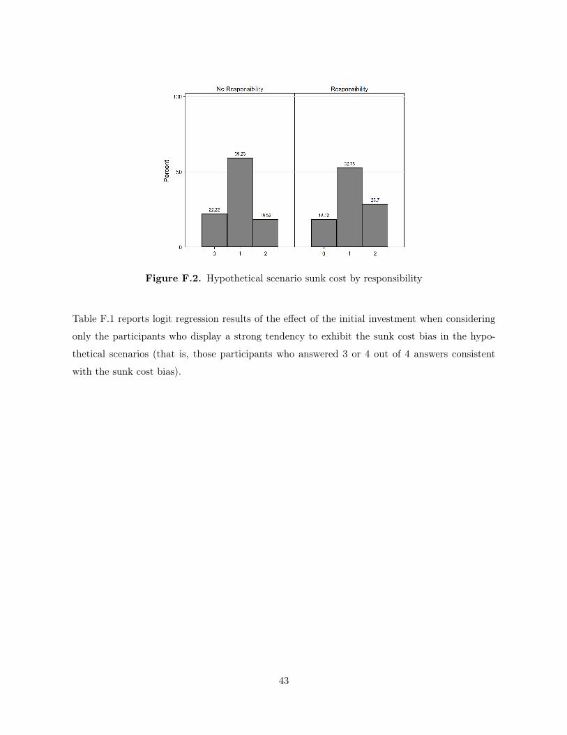
Figure F.2. Hypothetical scenario sunk cost by responsibility

Table F.1 reports logit regression results of the effect of the initial investment when considering

only the participants who display a strong tendency to exhibit the sunk cost bias in the hypo-

thetical scenarios (that is, those participants who answered 3 or 4 out of 4 answers consistent

with the sunk cost bias).

43

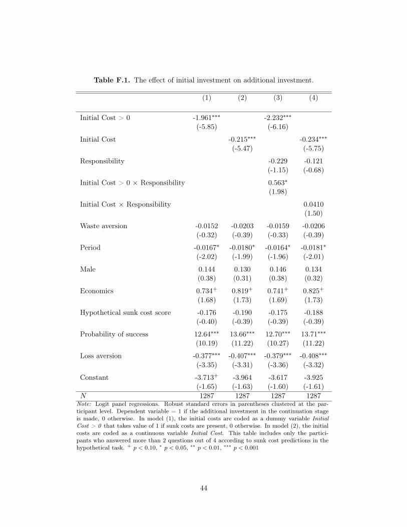
Table F.1. The effect of initial investment on additional investment.

(1) (2) (3) (4)

Initial Cost > 0 -1.961∗∗∗ -2.232∗∗∗

(-5.85) (-6.16)

Initial Cost -0.215∗∗∗ -0.234∗∗∗

(-5.47) (-5.75)

Responsibility -0.229 -0.121(-1.15) (-0.68)

Initial Cost > 0 × Responsibility 0.563∗

(1.98)

Initial Cost × Responsibility 0.0410(1.50)

Waste aversion -0.0152 -0.0203 -0.0159 -0.0206(-0.32) (-0.39) (-0.33) (-0.39)

Period -0.0167∗ -0.0180∗ -0.0164∗ -0.0181∗

(-2.02) (-1.99) (-1.96) (-2.01)

Male 0.144 0.130 0.146 0.134(0.38) (0.31) (0.38) (0.32)

Economics 0.734+ 0.819+ 0.741+ 0.825+

(1.68) (1.73) (1.69) (1.73)

Hypothetical sunk cost score -0.176 -0.190 -0.175 -0.188(-0.40) (-0.39) (-0.39) (-0.39)

Probability of success 12.64∗∗∗ 13.66∗∗∗ 12.70∗∗∗ 13.71∗∗∗

(10.19) (11.22) (10.27) (11.22)

Loss aversion -0.377∗∗∗ -0.407∗∗∗ -0.379∗∗∗ -0.408∗∗∗

(-3.35) (-3.31) (-3.36) (-3.32)

Constant -3.713+ -3.964 -3.617 -3.925(-1.65) (-1.63) (-1.60) (-1.61)

N 1287 1287 1287 1287Note: Logit panel regressions. Robust standard errors in parentheses clustered at the par-ticipant level. Dependent variable = 1 if the additional investment in the continuation stageis made, 0 otherwise. In model (1), the initial costs are coded as a dummy variable InitialCost > 0 that takes value of 1 if sunk costs are present, 0 otherwise. In model (2), the initialcosts are coded as a continuous variable Initial Cost. This table includes only the partici-pants who answered more than 2 questions out of 4 according to sunk cost predictions in thehypothetical task. + p < 0.10, ∗ p < 0.05, ∗∗ p < 0.01, ∗∗∗ p < 0.001

44

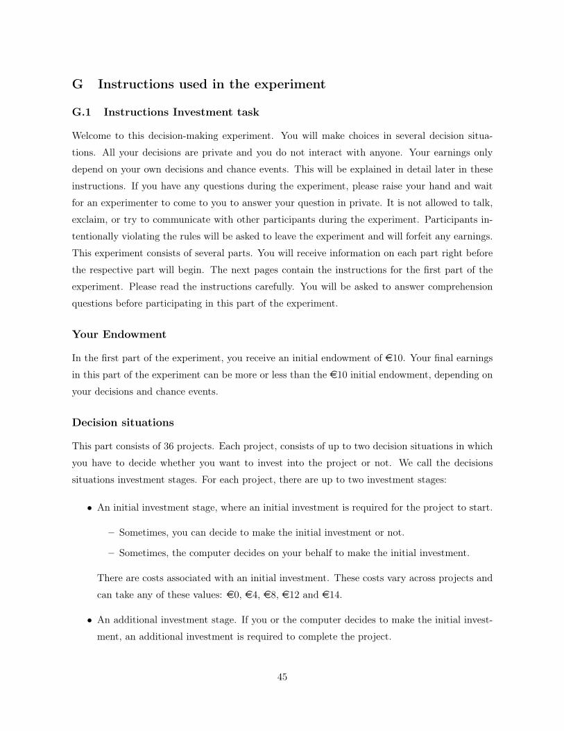
G Instructions used in the experiment

G.1 Instructions Investment task

Welcome to this decision-making experiment. You will make choices in several decision situa-

tions. All your decisions are private and you do not interact with anyone. Your earnings only

depend on your own decisions and chance events. This will be explained in detail later in these

instructions. If you have any questions during the experiment, please raise your hand and wait

for an experimenter to come to you to answer your question in private. It is not allowed to talk,

exclaim, or try to communicate with other participants during the experiment. Participants in-

tentionally violating the rules will be asked to leave the experiment and will forfeit any earnings.

This experiment consists of several parts. You will receive information on each part right before

the respective part will begin. The next pages contain the instructions for the first part of the

experiment. Please read the instructions carefully. You will be asked to answer comprehension

questions before participating in this part of the experiment.

Your Endowment

In the first part of the experiment, you receive an initial endowment of e10. Your final earnings

in this part of the experiment can be more or less than the e10 initial endowment, depending on

your decisions and chance events.

Decision situations

This part consists of 36 projects. Each project, consists of up to two decision situations in which

you have to decide whether you want to invest into the project or not. We call the decisions

situations investment stages. For each project, there are up to two investment stages:

• An initial investment stage, where an initial investment is required for the project to start.

– Sometimes, you can decide to make the initial investment or not.

– Sometimes, the computer decides on your behalf to make the initial investment.

There are costs associated with an initial investment. These costs vary across projects and

can take any of these values: e0, e4, e8, e12 and e14.

• An additional investment stage. If you or the computer decides to make the initial invest-

ment, an additional investment is required to complete the project.

45

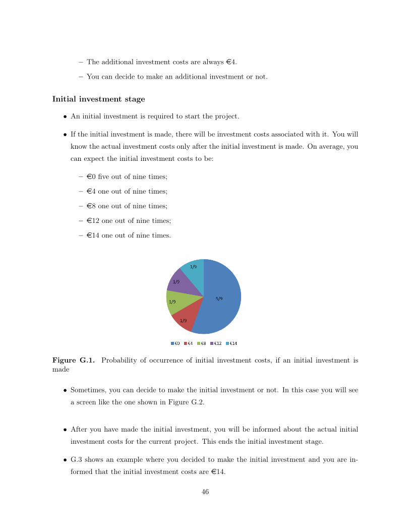
– The additional investment costs are always e4.

– You can decide to make an additional investment or not.

Initial investment stage

• An initial investment is required to start the project.

• If the initial investment is made, there will be investment costs associated with it. You will

know the actual investment costs only after the initial investment is made. On average, you

can expect the initial investment costs to be:

– e0 five out of nine times;

– e4 one out of nine times;

– e8 one out of nine times;

– e12 one out of nine times;

– e14 one out of nine times.

Figure G.1. Probability of occurrence of initial investment costs, if an initial investment ismade

• Sometimes, you can decide to make the initial investment or not. In this case you will see

a screen like the one shown in Figure G.2.

• After you have made the initial investment, you will be informed about the actual initial

investment costs for the current project. This ends the initial investment stage.

• G.3 shows an example where you decided to make the initial investment and you are in-

formed that the initial investment costs are e14.

46

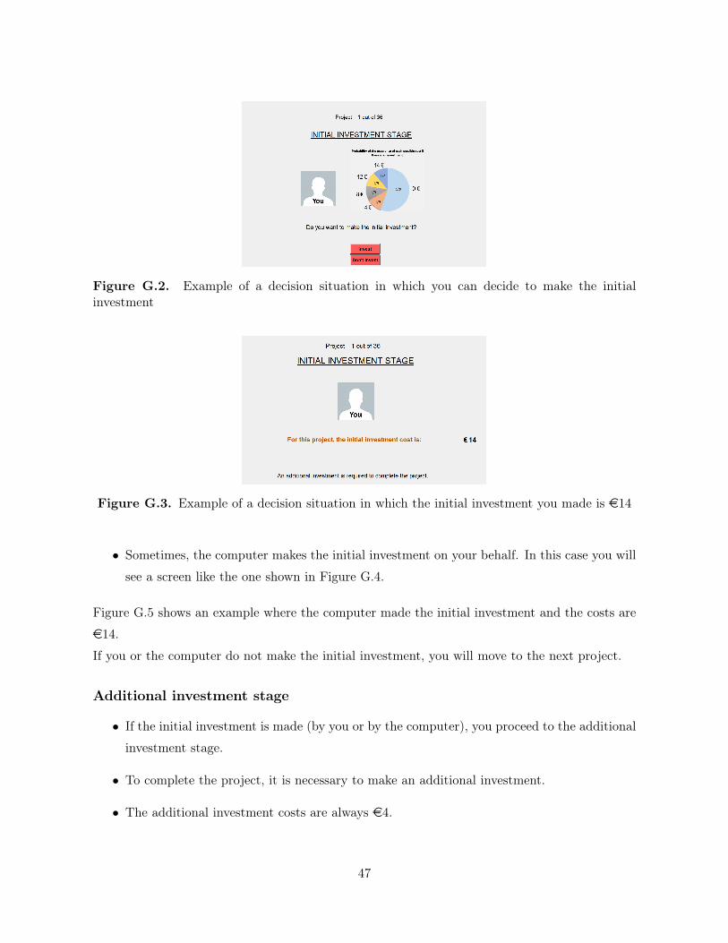
Figure G.2. Example of a decision situation in which you can decide to make the initialinvestment

Figure G.3. Example of a decision situation in which the initial investment you made is e14

• Sometimes, the computer makes the initial investment on your behalf. In this case you will

see a screen like the one shown in Figure G.4.

Figure G.5 shows an example where the computer made the initial investment and the costs are

e14.

If you or the computer do not make the initial investment, you will move to the next project.

Additional investment stage

• If the initial investment is made (by you or by the computer), you proceed to the additional

investment stage.

• To complete the project, it is necessary to make an additional investment.

• The additional investment costs are always e4.

47

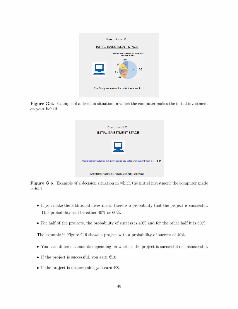
Figure G.4. Example of a decision situation in which the computer makes the initial investmenton your behalf

Figure G.5. Example of a decision situation in which the initial investment the computer madeis e14

• If you make the additional investment, there is a probability that the project is successful.

This probability will be either 40% or 60%.

• For half of the projects, the probability of success is 40% and for the other half it is 60%.

The example in Figure G.6 shows a project with a probability of success of 40%.

• You earn different amounts depending on whether the project is successful or unsuccessful.

• If the project is successful, you earn e16

• If the project is unsuccessful, you earn e8.

48

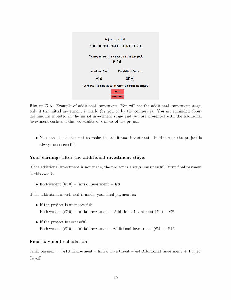
Figure G.6. Example of additional investment. You will see the additional investment stage,only if the initial investment is made (by you or by the computer). You are reminded aboutthe amount invested in the initial investment stage and you are presented with the additionalinvestment costs and the probability of success of the project.

• You can also decide not to make the additional investment. In this case the project is

always unsuccessful.

Your earnings after the additional investment stage:

If the additional investment is not made, the project is always unsuccessful. Your final payment

in this case is:

• Endowment (e10) – Initial investment + e8

If the additional investment is made, your final payment is:

• If the project is unsuccessful:

Endowment (e10) – Initial investment – Additional investment (e4) + e8

• If the project is successful:

Endowment (e10) – Initial investment– Additional investment (e4) + e16

Final payment calculation

Final payment = e10 Endowment - Initial investment – e4 Additional investment + Project

Payoff

49

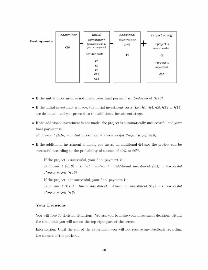
• If the initial investment is not made, your final payment is: Endowment (e10).

• If the initial investment is made, the initial investment costs (i.e., e0, e4, e8, e12 or e14)

are deducted, and you proceed to the additional investment stage.

• If the additional investment is not made, the project is automatically unsuccessful and your

final payment is:

Endowment (e10) – Initial investment + Unsuccessful Project payoff (e8).

• If the additional investment is made, you invest an additional e4 and the project can be

successful according to the probability of success of 40% or 60%.

– If the project is successful, your final payment is:

Endowment (e10) – Initial investment – Additional investment (e4) + Successful

Project payoff (e16)

– If the project is unsuccessful, your final payment is:

Endowment (e10) – Initial investment – Additional investment (e4) + Unsuccessful

Project payoff (e8)

Your Decisions

You will face 36 decision situations. We ask you to make your investment decisions within

the time limit you will see on the top right part of the screen.

Information: Until the end of the experiment you will not receive any feedback regarding

the success of the projects.

50

Payment

At the end of the experiment, one of the 36 decision situations will be randomly selected for

payout. Each decision situation is equally likely and your decisions in one decision situation

do not affect any other decision situation. Thus, each decision situation could be the one

relevant for your payment. Therefore, carefully consider your decisions in each decision

situation. The amount you earn will be transferred to your bank account at the end of the

experimental session. All bank transfers will be made on the same day of the experiment

by someone who is not directly involved in this study and who does not have access to the

data related to your decisions. Your anonymity is thus guaranteed.

Your Identity

For the entire duration of the experiment, your anonymity and the anonymity of all other

participants is guaranteed. You will never be asked to reveal your choices to other par-

ticipants during or after the experiment. Your decisions are thus private. Your name and

personal information are recorded only at the end of the experiment to pay you. To keep

your decisions private, please do not reveal your choices to any other participant. All the

interactions are anonymous and none of the participants can communicate or influence the

choices of the others.

This is the end of the instructions for Part 1. You can now answer the comprehension

questions. If you have any questions please raise your hand and wait for the experimenter.

G.2 Instructions loss aversion task

Welcome to this part of the experiment. You see below a list of lotteries. Each lottery consists

of a coin toss with 50% probability of success. You are asked to Accept or Reject each of these

lotteries. If you Accept the lottery, you can either win or lose money. This amount will be added

(if the lottery is successful) or subtracted (if the lottery fails) from the e7 you earned by answering

the questionnaire in the previous part of the experiment. If you Reject the lottery, you will neither

win nor lose money and you receive the e7 you earned by completing the questionnaire. At the

end of the experiment, one of the lotteries will be randomly selected for payout and you will be

paid according to your decision. Any earnings from this part of the experiment will be added

to your previous earnings, and will be transferred to your bank account after the end of this

experimental session.

Participants then saw the lotteries as in Table D.1.

51