econstorMake Your Publications Visible.

A Service of

zbwLeibniz-InformationszentrumWirtschaftLeibniz Information Centrefor Economics

Imas, Alex; Sadoff, Sally; Samek, Anya

Working Paper

Do People Anticipate Loss Aversion?

CESifo Working Paper, No. 5277

Provided in Cooperation with:Ifo Institute – Leibniz Institute for Economic Research at the University of Munich

Suggested Citation: Imas, Alex; Sadoff, Sally; Samek, Anya (2015) : Do People Anticipate LossAversion?, CESifo Working Paper, No. 5277, Center for Economic Studies and ifo Institute(CESifo), Munich

This Version is available at:http://hdl.handle.net/10419/110779

Standard-Nutzungsbedingungen:

Die Dokumente auf EconStor dürfen zu eigenen wissenschaftlichenZwecken und zum Privatgebrauch gespeichert und kopiert werden.

Sie dürfen die Dokumente nicht für öffentliche oder kommerzielleZwecke vervielfältigen, öffentlich ausstellen, öffentlich zugänglichmachen, vertreiben oder anderweitig nutzen.

Sofern die Verfasser die Dokumente unter Open-Content-Lizenzen(insbesondere CC-Lizenzen) zur Verfügung gestellt haben sollten,gelten abweichend von diesen Nutzungsbedingungen die in der dortgenannten Lizenz gewährten Nutzungsrechte.

Terms of use:

Documents in EconStor may be saved and copied for yourpersonal and scholarly purposes.

You are not to copy documents for public or commercialpurposes, to exhibit the documents publicly, to make thempublicly available on the internet, or to distribute or otherwiseuse the documents in public.

If the documents have been made available under an OpenContent Licence (especially Creative Commons Licences), youmay exercise further usage rights as specified in the indicatedlicence.

www.econstor.eu

Do People Anticipate Loss Aversion?

Alex Imas Sally Sadoff Anya Samek

CESIFO WORKING PAPER NO. 5277 CATEGORY 13: BEHAVIOURAL ECONOMICS

MARCH 2015

An electronic version of the paper may be downloaded • from the SSRN website: www.SSRN.com • from the RePEc website: www.RePEc.org

• from the CESifo website: Twww.CESifo-group.org/wp T

ISSN 2364-1428

CESifo Working Paper No. 5277

Do People Anticipate Loss Aversion?

Abstract There is growing interest in the use of loss contracts that offer performance incentives as upfront payments that employees can lose. Standard behavioral models predict a tradeoff in the use of loss contracts: employees will work harder under loss contracts than under gain contracts; but, anticipating loss aversion, they will prefer gain contracts to loss contracts. In a series of experiments, we test these predictions by measuring performance and preferences for payoff-equivalent gain and loss contracts. We find that people indeed work harder under loss than gain contracts, as the theory predicts. Surprisingly, rather than a preference for the gain contract, we find that people actually prefer loss contracts. In exploring mechanisms for our results, we find suggestive evidence that people do anticipate loss aversion but select into loss contracts as a commitment device to improve performance.

JEL-Code: D030.

Alex Imas Social and Decision Sciences Carnegie Mellon University

5000 Forbes Avenue, 319C Porter Hall USA - 15213 Pittsburgh PA

aimas@andrew.cmu.edu

Sally Sadoff* University of California San Diego

Rady School of Management Wells Fargo Hall, Room 4W121

9500 Gilman Drive #0553 USA - La Jolla, CA 92093-0553

ssadoff@ucsd.edu

Anya Samek

University of Wisconsin-Madison School of Human Ecology 4214 Nancy Nicholas Hall

1300 Linden Drive USA - Madison, WI 53706

asamak@wisc.edu *corresponding author March, 2014 This Version: March 10, 2015 We thank Christa Gibbs and Stephanie Schwartz for providing truly outstanding research assistance. This research has been conducted with IRB approval.

1 Introduction

Attempts to take advantage of findings from behavioral economics have become in-

creasingly popular in management and public policy (Madrian, 2014). A prime ex-

ample is the phenomenon of loss aversion, which predicts that gains and losses are

evaluated relative to a reference point, and that losses loom larger than gains.1 An

important behavioral prediction of loss aversion is that individuals first endowed with

a payment will work harder to avoid losing it than to earn the same amount presented

as a gain. Recent work has explored whether the design of incentive contracts can

exploit this insight to increase e↵ort and performance in the workplace (Hossain and

List, 2012; Fryer et al., 2012). These studies find that presenting incentives in the form

of loss contracts (i.e., bonuses workers could potentially lose) increases productivity

relative to payo↵-equivalent gain contracts where the same bonuses are presented as

gains.

A natural criticism of the economic significance of loss contracts is that if people

are averse to losses, they will have a preference for gain contracts. In turn, firms may

have to pay a premium for workers to accept loss contracts, which could outweigh

their productivity benefits and make loss contracts ine�cient. As we discuss further

in the next section, a standard behavioral model of reference-dependent preferences

makes two central predictions: first, in order to avoid potential losses, individuals will

exert more e↵ort under a loss contract than a gain contract; and second, anticipating

this loss aversion, individuals will have a strict preference for the gain contract.2

1Kahneman and Tversky’s (1979) seminal work on prospect theory introduced and formalizedloss aversion. Since then, loss aversion has been used to explain a variety of behavioral anomaliesincluding the endowment e↵ect (Kahneman, Knetsch and Thaler, 1990) and status quo bias (Samuel-son and Zeckhauser, 1988). For recent reviews of applications of reference dependent preferences,see Camerer et al. (2004), DellaVigna (2009), Barberis (2013) and Ericson and Fuster (2014).

2Models using the status-quo as the reference point (e.g., Thaler and Johnson, 1990) predictthat individuals will work harder under loss-framed contracts conditional on the endowment beingincorporated as the status-quo. If the expectation is taken as the reference point (e.g., Koszegi and

2

The intuition is that because losses are painful, people will work harder to avoid

losing a bonus than they would to receive the same bonus o↵ered as a gain. At the

same time, working harder than is otherwise optimal in order to avoid losses lowers

expected utility relative to working under a gain contract. If employees anticipate

this di↵erence in expected utility, they will demand a wage premium to work under

a loss contract, which may o↵set the prospective productivity gains. As discussed

above, several recent studies have provided evidence for the first prediction – that loss

contracts increase workplace productivity (Brooks, Stremitzer, and Tontrup, 2011;

Hossain and List 2012; Fryer et al., 2012).3 However, less work has been done to

directly investigate the second prediction, that individuals have a preference for gain

contracts over loss contracts. Understanding individuals’ preferences over contracts

is critical to determining optimal contract design from the perspective of the firm or

manager.

In this paper, we present results from a series of incentivized laboratory exper-

iments that test how gain and loss contracts a↵ect productivity, and measure the

ex ante preferences for selecting into payo↵-equivalent gain and loss contracts for

the same task. We first test whether participants exert greater e↵ort when payo↵-

equivalent incentives are presented as a loss contract rather than a gain contract. We

then conduct a second experiment to examine whether people anticipate the di↵er-

ential e↵ect of the loss contract in line with the standard behavioral model – that

is, whether they prefer gain rather than loss contracts. To do this, we use the same

task and compare participants’ willingness to pay (WTP) to work under the loss con-

Rabin, 2006), then no di↵erence between the frames should be observed either in e↵ort or in contractpreference. As such, in our context, a “standard behavioral model” refers to models assuming thestatus quo as the reference point.

3Note that field studies in some other contexts including incentives for student performance(Levitt et al., 2012) and child food choice (List and Samek, 2014) have not found significant di↵er-ences in e↵ort in loss and gain frames.

3

tract versus their WTP to work under the gain contract. Finally, we investigate the

correlation of performance and selection into contracts with a separately elicited loss

aversion parameter.4

In line with the standard model of prospect theory, we find that individuals as-

signed to the loss contract work harder than those assigned to the gain contract.

However, we do not find support for the theoretical prediction that people prefer the

gain contract to the loss contract. Surprisingly, people are willing to pay more to

enter the loss contract than to enter the payo↵-equivalent gain contract for the same

task. We conclude that participants do not anticipate the di↵erential e↵ects of the

loss contract in the direction predicted by standard behavioral theory.

To shed light on the mechanisms behind our results, we examine the relationship

between performance, contract preferences and the separately elicited individual-level

loss aversion parameter. We test the predictions of the standard behavioral model

that more loss averse people are more sensitive to loss contracts. First, we test

that performance under loss contracts is increasing in an individual’s degree of loss

aversion, and second that WTP for loss contracts is decreasing in an individual’s

degree of loss aversion. As discussed above, losses are more painful for people who

are more loss averse and this leads to two predictions: greater loss aversion leads to

greater e↵ort when assigned to a loss contract, and this greater e↵ort corresponds

to lower expected welfare ex ante. In turn, if people anticipate their degree of loss

aversion when selecting into a contract, more loss averse people will have a greater

ex ante preference against loss contracts.

We find suggestive evidence to support the first prediction: performance under

loss contracts increases with the degree of loss aversion while loss aversion has no

4Prior to conducting the experiments, we ran a series of pilots with a smaller sample, which aresummarized in Appendix B. The results of the pilot experiments are consistent with the findings ofthe experiments reported here.

4

relationship with performance under the gain contract. However, we find no evi-

dence for the second prediction; rather, willingness to pay for loss contracts seems

to increase rather than decrease with the degree of loss aversion. As discussed in

Section 6, our findings may provide support for a behavioral model that incorporates

dynamic inconsistency in preferences. Particularly, in this framework loss contracts

can be viewed as a commitment device which (sophisticated) workers select in order

to improve their performance and thus increase their expected earnings. Those who

are most sensitive to losses (i.e., the most loss averse) will both work hardest and

have the highest WTP for loss contracts – consistent with our empirical results.

The few prior studies examining contract preferences in this context have found

mixed evidence on selection into loss and gain contracts. Luft (1994) examines entry

into gain and loss contracts (with an emphasis on calling them ‘bonus’ and ‘penalty’

contracts), and finds that participants are more likely to enter into contracts framed

as gains. More recently, Brooks et al. (2014) find that entry rates for loss contracts

are lower than gain contracts when the performance threshold is very high. In work

conducted concurrently to our own, de Quidt (2014) examines the e↵ect of framing on

entry into contracts o↵ered on the crowdsourcing platform Amazon Mechanical Turk.

In line with our empirical results, but in contrast to standard behavioral theory, de

Quidt (2014) finds that entry rates are higher in the loss-framed contract than in

the gain-framed contract. To our knowledge, ours is the only study to separately ex-

amine preferences between contracts and the e↵ect of contract type on productivity.

This allows us to identify the role of loss aversion in both contract preference and

productivity without issues of selection e↵ects (which our results suggest could be a

potentially serious confound). Ours is also the first study to investigate how perfor-

mance and contract preferences vary by individuals’ degree of loss aversion, which

5

allows us to identify potential mechanisms driving the results.5

The remainder of the paper is organized as follows. In Section 2, we discuss four

theoretical predictions of a simple behavioral model of reference dependent preferences

and loss aversion, which motivate our experimental design and analysis. Section 3

presents the design and results of our first experiment, which separately identifies

the e↵ect of contract type on productivity. Section 4 presents our second experiment

investigating preferences over gain versus loss contracts. Section 5 describes our

elicitation of an individual-level loss aversion parameter and subsequent tests. Section

6 discusses implications of the results, and Section 7 concludes.

2 Theoretical Predictions

We consider a standard behavioral model in which people derive additively separable

utility from consumption net of costs, net consumption utility, as in the standard

framework; and also derive gain-loss utility relative to a reference point, as in the

prospect theory model. We assume the reference point is determined by the status

quo (e.g., Thaler and Johnson, 1990). In our context, a performance incentive can be

o↵ered as a gain, in which the status quo is not having the incentive, or as a potential

loss, in which the status quo is having the incentive. In gain contracts, people work to

increase the probability they will receive the incentive. In loss contracts, people work

to increase the probability they will avoid losing the incentive. There are two critical

assumptions of this model. First, people experience utility relative to a reference

point, deriving positive gain-loss utility from gains and negative gain-loss utility from

5De Quidt (2014) includes an unincentivized survey measure of risk preferences using hypotheticallotteries. Unlike our incentivized measure, this survey measure does not separately identify lossaversion from utility curvature in the gain and loss domains, and hence cannot be used as a clean testof the theory. Additionally, individuals who selected out of participating in the loss or gain contractdid not complete the survey, making it di�cult to examine the relationship between individuals’degree of risk preferences and selection into contracts.

6

losses (Kahneman and Tversky, 1979); utility from remaining at the reference point

is normalized to zero. Second, losses loom larger than gains such that the negative

gain-loss utility from a loss of x relative to the reference point is larger in absolute

value than the positive gain-loss utility from a gain of x. This greater sensitivity

to losses – loss aversion – leads to our first two predictions for relative performance

under gain versus loss contracts. See Appendix A for proofs of all results.

Prediction 1: If people are loss averse, performance will be higher under a loss

contract than a gain contract.

Under both a gain and loss contract, individuals choose optimal e↵ort to maximize

expected utility – i.e., the e↵ort level at which the marginal benefits from increasing

the likelihood of earning the incentive equal the marginal costs. Both contract types

have identical marginal costs of e↵ort and identical marginal benefits to consumption

utility, and thus identical marginal benefits to net consumption utility. Where they

di↵er is in their marginal benefits to gain-loss utility, which in the gain contract is

the increased likelihood of experiencing a pleasant gain and in the loss contract is the

increased likelihood of avoiding an unpleasant loss. If people are loss averse, the gain-

loss utility from avoiding the loss is greater than the gain-loss utility from obtaining

the gain. In turn, the marginal benefit of e↵ort under loss contracts is greater than

under gain contracts. People will therefore work harder under the loss contract than

the gain contract.

Prediction 2: Among people who are loss averse, performance di↵erences between

contracts are increasing in individuals’ degree of loss aversion.

As discussed above, a greater sensitivity to losses than gains leads to performance

di↵erences between gain and loss contracts. Larger di↵erences in sensitivity will lead

7

to larger di↵erences in performance. If a person is not at all loss averse, she is equally

sensitive to gains and losses and her performance will not di↵er between contracts.6

Our next two behavioral predictions concern preferences over gain and loss con-

tracts. We consider the decision between selecting into a contract and potentially

earning the incentive, or accepting a fixed payment. The highest amount someone is

willing to forgo in order to participate in the contract is her willingness to pay (WTP).

A person’s WTP is determined by her maximum expected utility from working under

the contract – i.e., exerting the optimal level of e↵ort as discussed in Prediction 1.

Prediction 3: If people have dynamically consistent preferences and rational expec-

tations, willingness to pay for the gain contract will be higher than willingness to pay

for the loss contract.

Under the behavioral model, expected utility is the sum of expected net con-

sumption utility plus expected gain-loss utility. We first compare expected gain-loss

utility across contracts. Gain-loss utility is positive for gains and negative for losses.

As such, gain-loss utility is always (weakly) greater under gain contracts than loss

contracts. This is because the worst a person can do under a gain contract is not

receive the incentive; if she does not receive the incentive, the agent will remain at her

reference point and derive zero gain-loss utility. Any positive probability of earning

the incentive increases her expected gain-loss utility above zero. In contrast, under

loss contracts the best a person can do is to keep the incentive – she will remain at

her reference point and derive zero gain-loss utility. Any positive probability that she

does not earn the incentive decreases her expected gain-loss utility below zero.

We now compare expected net consumption utility across contracts, which is the

expected consumption utility minus e↵ort costs as in the standard Expected Utility

6If a person is less sensitive to losses than she is to gains, performance will be higher under gaincontracts and the gain-loss gap will increase as loss sensitivity decreases.

8

model:

e[u(b)]� c(e) (1)

where the probability of earning the incentive b > 0 equals e↵ort e 2 (0, 1), u(·) is

consumption utility from the incentive and c(·) is the cost of e↵ort. We assume u is

increasing and concave and c is increasing and convex, and we normalize consumption

utility from not receiving the incentive to zero. Let e⇤S maximize (1). As discussed in

Prediction 1, optimal e↵ort under the loss contract e

⇤L will be greater than optimal

e↵ort under the gain contract e

⇤G. By the same logic, e⇤G will be greater than e

⇤S

(because e↵ort increases the marginal benefits to gain-loss utility). Because e↵ort

under the gain contract e⇤G does not equal e⇤S, it cannot maximize (1) – in particular,

it is too high. E↵ort under the loss contract e⇤L is even farther from maximizing (1),

as it is higher than e

⇤G. Thus, e⇤Su(b) � c(e⇤S) > e

⇤Gu(b) � c(e⇤G) > e

⇤Lu(b) � c(e⇤L).

Expected net consumption utility is higher under gain contracts than loss contracts.

Note that because e↵ort is higher under loss contracts than gain contracts, ex-

pected earnings will also be higher. However, this increase in e↵ort represents a

distortion from what is otherwise optimal from the perspective of maximizing con-

sumption utility net of e↵ort costs. It occurs because people are trying to compensate

for the negative expected gain-loss utility imposed by facing the threat of potential

losses.

Both expected gain-loss utility and expected net consumption utility are lower

in loss contracts than gain contracts. If people have rational expectations, they will

anticipate this di↵erence and will have a higher willingness to pay for a gain contract

than a loss contract. If people do not have rational expectations regarding their degree

of loss aversion, and in turn, the di↵erential e↵ect of the loss contract on behavior,

they will expect their reference point and optimal e↵ort under the loss contract to be

9

the same as it is under the gain contract. In this case, willingness to pay for the loss

contract will be equal to willingness to pay for the gain contract.

Prediction 4: If people are dynamically consistent and have rational expectations,

di↵erences in willingness to pay will be larger among people who are more loss averse.

As discussed above, a greater sensitivity to losses than gains decreases WTP for

loss contracts through both a decrease in gain-loss utility and a distortion in e↵ort

(relative to gain-loss utility and e↵ort under gain contracts). Larger di↵erences in

sensitivity lead to larger gaps in WTP for a gain contract compared to a loss contract.

Note that this model assumes that people are dynamically consistent. That is, the

preferences of a person when choosing the contract are consistent with her preferences

when working under a contract. As we discuss further in Section 6, individuals who

have dynamically inconsistent preferences – where the relative weight placed on the

cost of e↵ort is disproportionately greater in the period the individual has to work

than in the preceding periods – may actually prefer loss contracts as commitment

devices to induce their future selves to work harder.

3 Experiment 1: E↵ort under gain and loss con-

tracts

3.1 Experimental Design

To test whether people anticipate loss aversion, we first need to establish that individ-

ual e↵ort is indeed di↵erentially a↵ected by the two contract types, which is what we

set out to do in our first experiment. Experiment 1 was implemented with 83 subjects

at Carnegie Mellon University (CMU), with 4-8 subjects in each session. Subjects

were randomized at the session level to either a GAIN or LOSS treatment, which

corresponded to working under a gain contract or a loss contract, respectively. Then,

10

subjects participated in a real-e↵ort task where we o↵ered them an incentive based

on their performance. Performance in the real-e↵ort task is the primary outcome

measure in Experiment 1.

Upon arriving at the lab, subjects were assigned to a private computer station

and given the instructions for the real-e↵ort task, which were also read out loud.

We used a one-shot version of the slider task developed and validated by Gill and

Prowse (2012). In this task, subjects complete a series of sliders by moving them

sequentially on their computer screen to an assigned point along a bar using their

computer mouse. Subjects were incentivized to complete as many sliders as possible

(max 30) in 1.5 minutes (see Appendix C for instructions and a screen shot of the

task).

All subjects were o↵ered a non-monetary incentive for completing more sliders

than a previously determined exogenous threshold. In both treatments, the threshold

was the average performance of subjects who previously completed the same task for

a piece-rate.7 In both treatments, the incentive was a custom made T-shirt with an

unknown outside value and a subjective personal value (its actual cost was about

$8). The exogenous threshold, which was the same for both the GAIN and LOSS

treatments, assures that expectations about the level of e↵ort required to end up with

the incentive does not vary by treatment and does not depend on beliefs about the

performance of other participants in the experiment. The value of the threshold was

also unknown to subjects in advance, and hence beliefs were such that any increase

in performance should increase the probability of ending up with the incentive.

In the GAIN treatment, the experimenter held up the T-shirt at the front of the

7Subjects were told that the threshold was determined by the average performance of a group ofCMU students who worked on the same task but who were paid cash based on their performance.The previous group had worked on the task in the previous year, earning $0.50 per completed slider.Average earnings in the previous task were $9.50, which is similar to the cost of the non-financialincentive we o↵ered participants in our experiment.

11

room and told subjects that they would receive it if their performance on the slider

task was equal to or above the threshold; otherwise they would receive nothing. In

the LOSS treatment, participants were first given the T-shirt, which remained at

their station throughout the session. The experimenter told subjects that they would

keep the T-shirt if their performance was equal to or above the threshold; otherwise

they would have to return it. This design created two contracts that were equivalent

in payo↵s - requiring the same level of e↵ort to end up with the incentive. However,

in the GAIN treatment the contract incentivized participants to work to gain the

payo↵, whereas the LOSS treatment incentivized participants to work to avoid losing

the same payo↵. After learning about the incentive scheme, subjects performed the

slider task.

At the end of the real-e↵ort task, but before participants learned whether they

earned the T-shirt, we endowed all participants with an additional $10 and elicited

individual loss aversion parameters using a multiple price list (we discuss details and

results in Section 5). After completing the experiment, subjects filled out a short

survey and received payment from the task including a pre-announced show-up fee of

$5. Participation in Experiment 1 took about 25 minutes.

3.2 Results

The behavioral model presented in Section 2 predicts that if people are loss averse, the

number of sliders completed (performance) will be higher under a loss contract than

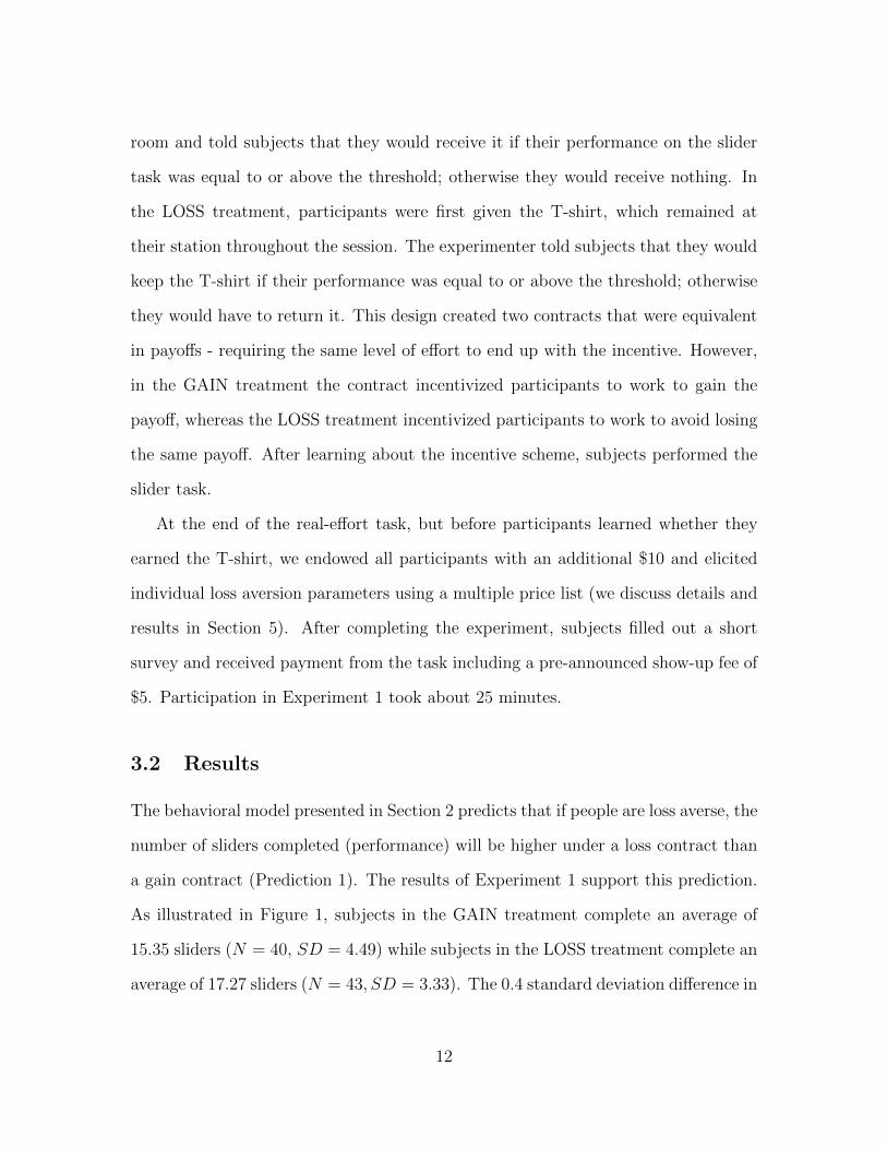
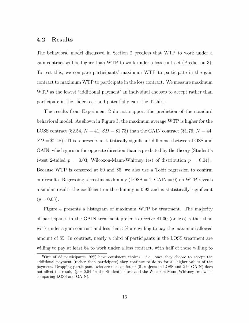
a gain contract (Prediction 1). The results of Experiment 1 support this prediction.

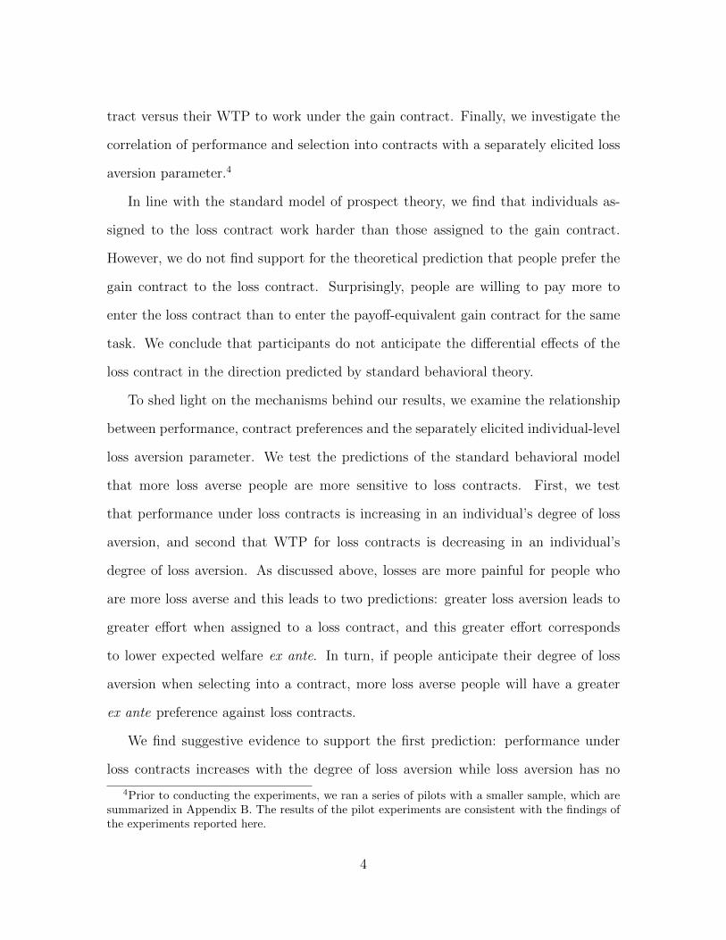
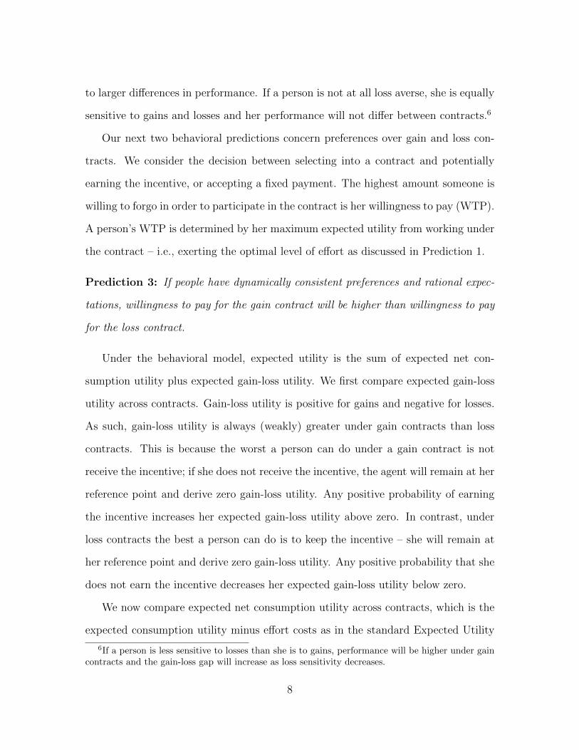
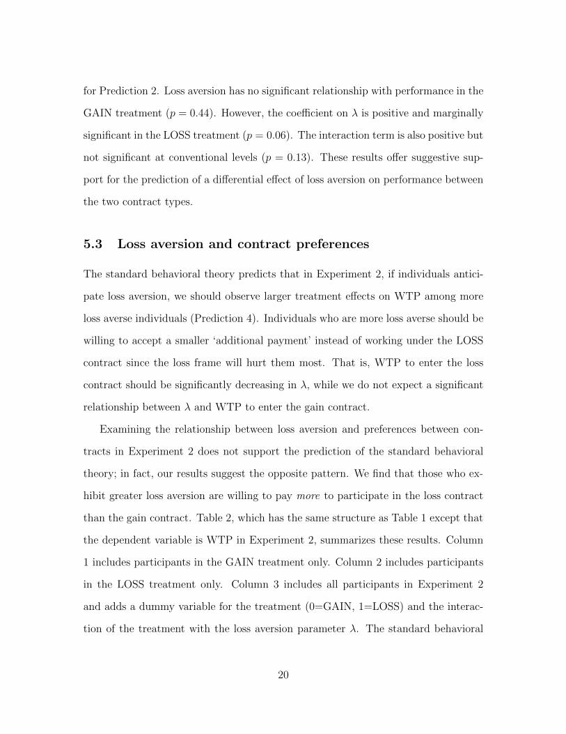
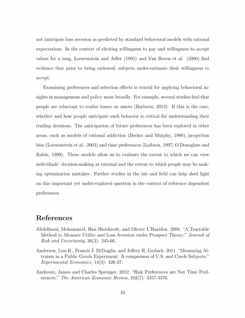
As illustrated in Figure 1, subjects in the GAIN treatment complete an average of

15.35 sliders (N = 40, SD = 4.49) while subjects in the LOSS treatment complete an

average of 17.27 sliders (N = 43, SD = 3.33). The 0.4 standard deviation di↵erence in

12

performance is statistically significant (Student’s t-test 2-tailed p = 0.03, Wilcoxon-

Mann-Whitney test of distribution p = 0.05).

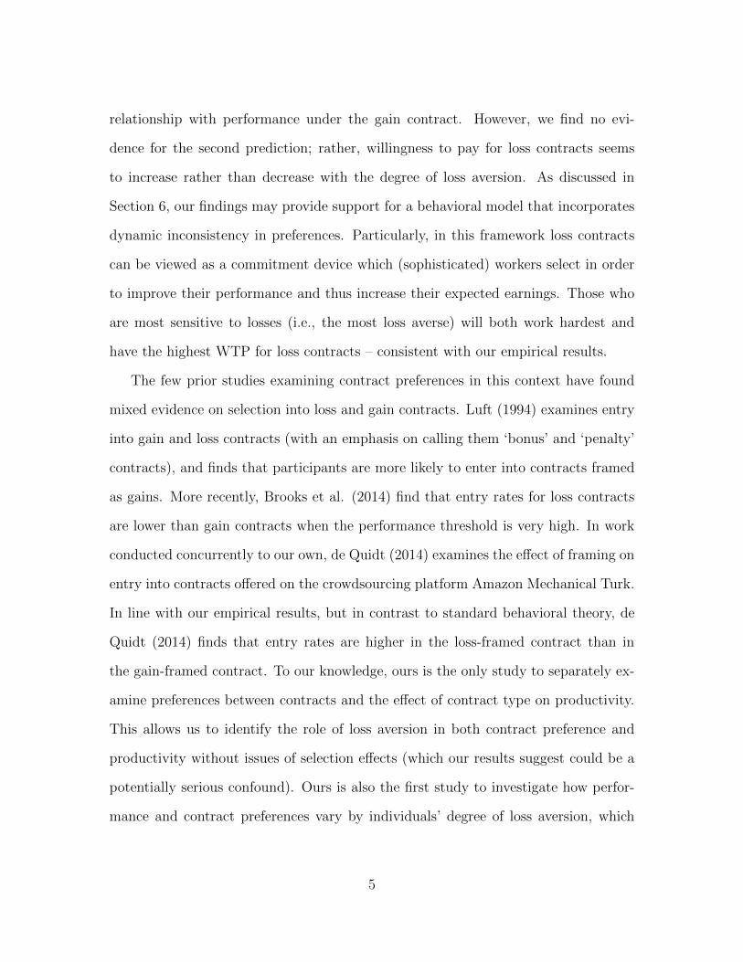
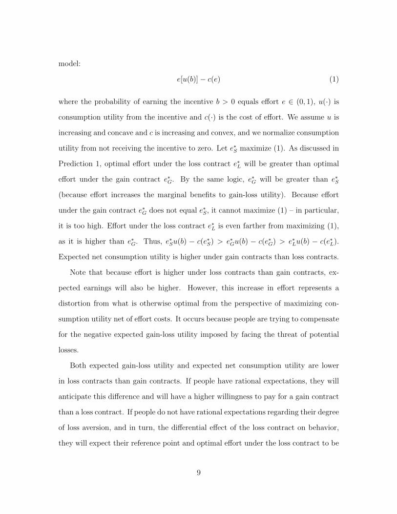
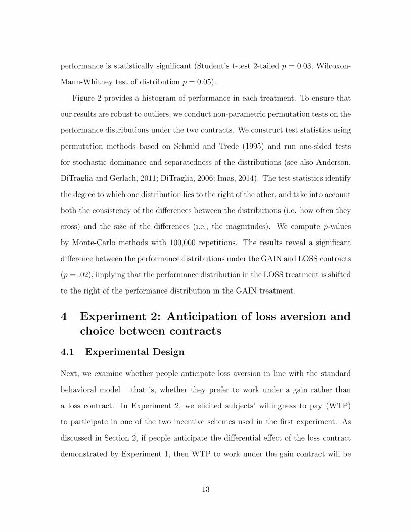
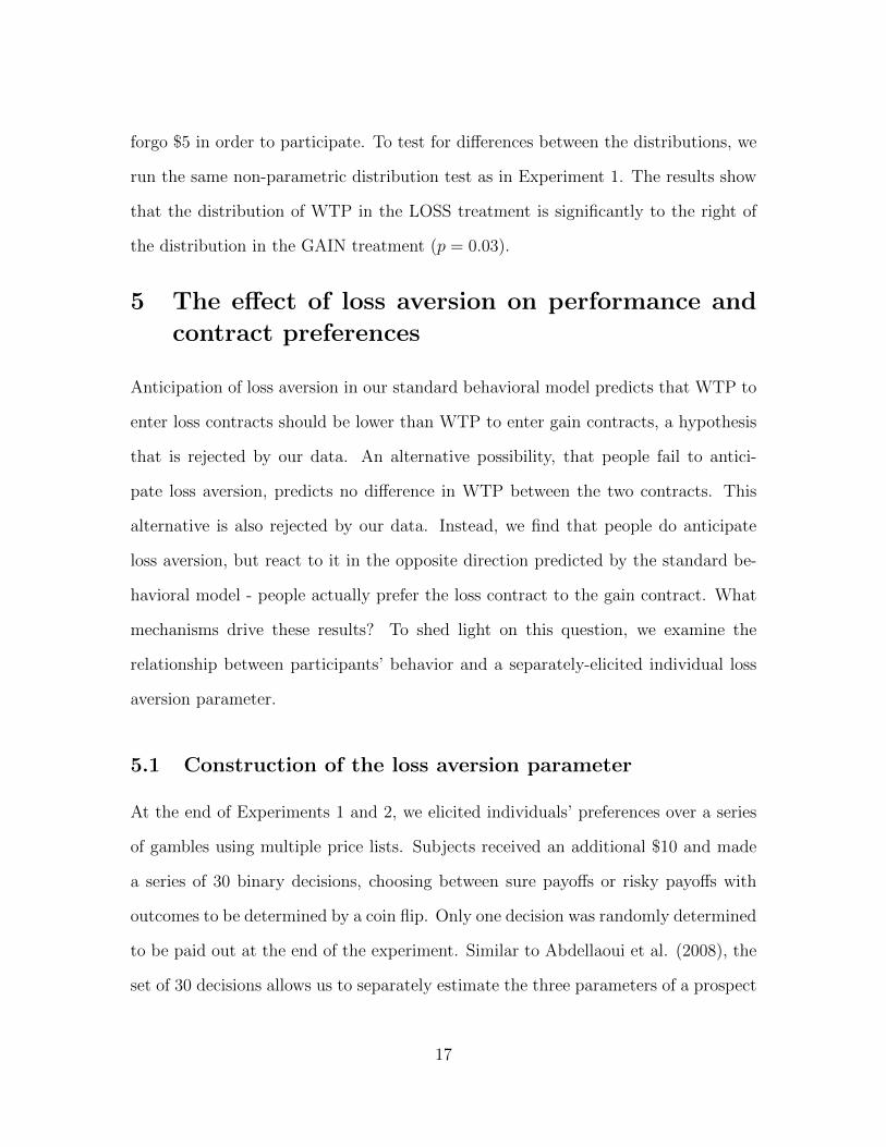
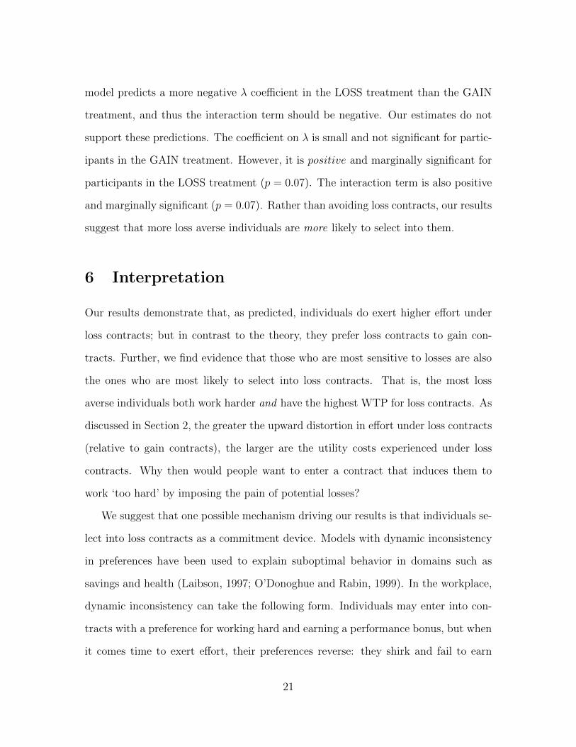
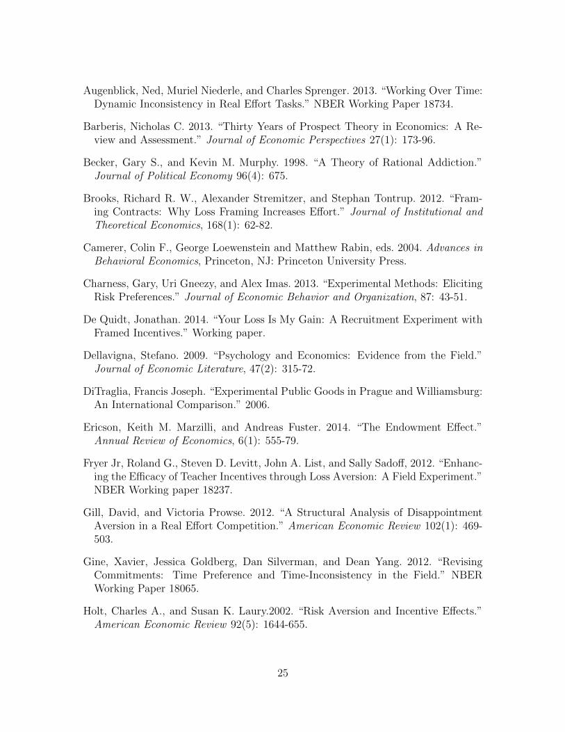
Figure 2 provides a histogram of performance in each treatment. To ensure that

our results are robust to outliers, we conduct non-parametric permutation tests on the

performance distributions under the two contracts. We construct test statistics using

permutation methods based on Schmid and Trede (1995) and run one-sided tests

for stochastic dominance and separatedness of the distributions (see also Anderson,

DiTraglia and Gerlach, 2011; DiTraglia, 2006; Imas, 2014). The test statistics identify

the degree to which one distribution lies to the right of the other, and take into account

both the consistency of the di↵erences between the distributions (i.e. how often they

cross) and the size of the di↵erences (i.e., the magnitudes). We compute p-values

by Monte-Carlo methods with 100,000 repetitions. The results reveal a significant

di↵erence between the performance distributions under the GAIN and LOSS contracts

(p = .02), implying that the performance distribution in the LOSS treatment is shifted

to the right of the performance distribution in the GAIN treatment.

4 Experiment 2: Anticipation of loss aversion and

choice between contracts

4.1 Experimental Design

Next, we examine whether people anticipate loss aversion in line with the standard

behavioral model – that is, whether they prefer to work under a gain rather than

a loss contract. In Experiment 2, we elicited subjects’ willingness to pay (WTP)

to participate in one of the two incentive schemes used in the first experiment. As

discussed in Section 2, if people anticipate the di↵erential e↵ect of the loss contract

demonstrated by Experiment 1, then WTP to work under the gain contract will be

13

higher than WTP to work under the loss contract (Prediction 3). The elicited WTP

is the primary outcome measure for Experiment 2.

Experiment 2 was implemented using 85 subjects at CMU, with 4-8 subjects in

each session. Using a between-subject design, we randomized subjects to one of the

two treatments described in Experiment 1: GAIN or LOSS. As in Experiment 1,

subjects were randomized to treatment at the session level. Unlike in Experiment 1,

rather than simply participating in the real-e↵ort task, subjects were asked to indicate

their WTP to participate.

Upon arriving at the lab, subjects were assigned to a private computer station and

given the instructions, which were also read out loud. The experiment proceeded in

two parts. In the first part, we explained the slider task (using the same instructions

as in Experiment 1), and then elicited WTP to participate in the slider task with the

T-shirt as the incentive. In both the GAIN and LOSS treatments, the experimenter

held up the T-shirt at the front of the room and read the instructions describing

either the gain or the loss contract from Experiment 1.

To elicit WTP, we asked subjects to make a series of trade-o↵s between either

working under the respective contract (GAIN or LOSS) or receiving a sum of money.8

We used a multiple price list, which has been employed as an incentive-compatible

method to elicit attitudes for risk (Holt and Laury, 2002; Sprenger, 2013; Char-

ness, Gneezy and Imas, 2013) and time preferences (Andersen et al. 2007). In our

paradigm, participants made a series of decisions between either participating in the

task or not participating and receiving an ‘additional payment’ at the end of the

experiment. The additional payment was $0 for the first decision and increased to $5

8In this design, subjects are paying to participate with the foregone payo↵ from not participating.This is more natural for subjects who are used to earning money, rather than spending money, toparticipate in experiments. In addition, it models the opportunity costs employees are willing toforego in order to enter a contract and matches the theoretical model discussed in Section 2.

14

by the last decision in increments of $0.50 (see Appendix C for instructions).

We used a die roll to randomly choose a single decision from the list to be im-

plemented. The additional payment o↵ered in the implemented decision determined

the opportunity cost of working under the contract. If a subject had indicated that

she was willing to forego the payment and participate, then she participated and

received no additional compensation. If a subject indicated she preferred to receive

the payment, then she waited at the computer terminal during the 1.5 minutes of the

task instead of participating (and received the additional payment at the end of the

experiment).

In the second part of the experiment, those who were willing to pay the randomly

selected cost participated in the contract described in Experiment 1. In the GAIN

treatment, those who elected to participate completed the slider task and received the

T-shirt if their performance was equal to or above the performance threshold. Those

who opted to participate in the LOSS treatment were first given the T-shirt to keep at

their desk, performed the slider task, and got to keep the T-shirt if their performance

was equal to or above the threshold, or had to return it if their performance was

below the threshold. Those who opted not to participate waited at their computer

terminals until the slider task was complete.

Finally, at the end of the experiment (before participants learned whether they

earned the T-shirt) we elicited individual loss aversion parameters. As in Experiment

1, we endowed all participants with an additional $10 and used multiple price lists,

which we describe in detail in Section 5. At the end of the session, all participants filled

out a short survey and received their pre-announced $5 show-up fee plus additional

payments earned in the experiment. The session lasted approximately 45 minutes.

15

4.2 Results

The behavioral model discussed in Section 2 predicts that WTP to work under a

gain contract will be higher than WTP to work under a loss contract (Prediction 3).

To test this, we compare participants’ maximum WTP to participate in the gain

contract to maximumWTP to participate in the loss contract. We measure maximum

WTP as the lowest ‘additional payment’ an individual chooses to accept rather than

participate in the slider task and potentially earn the T-shirt.

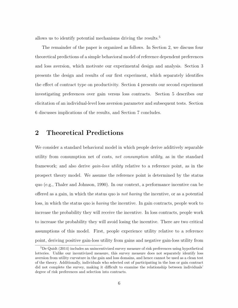
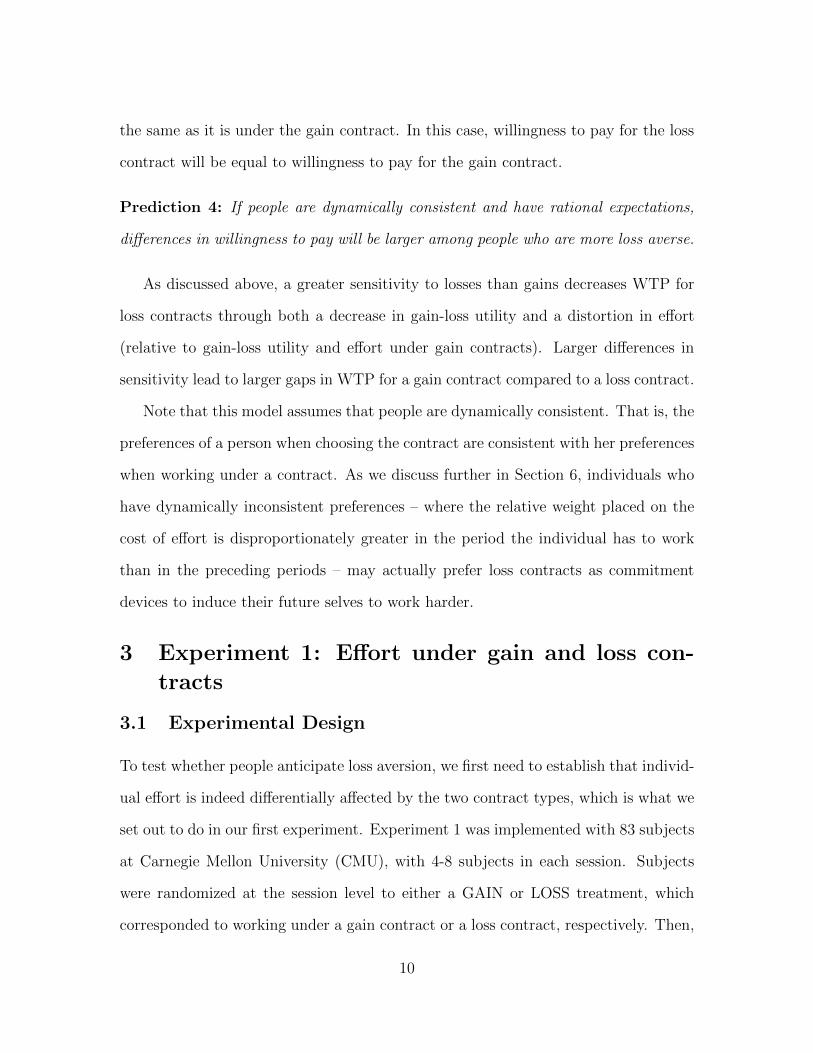
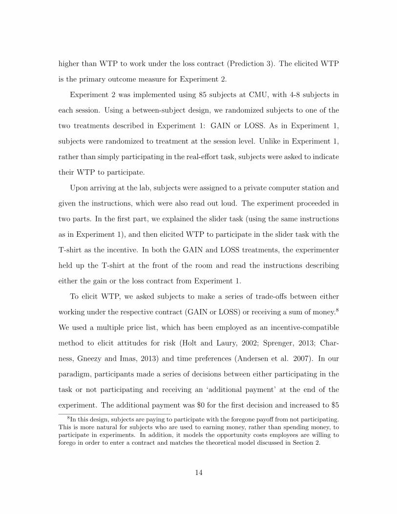
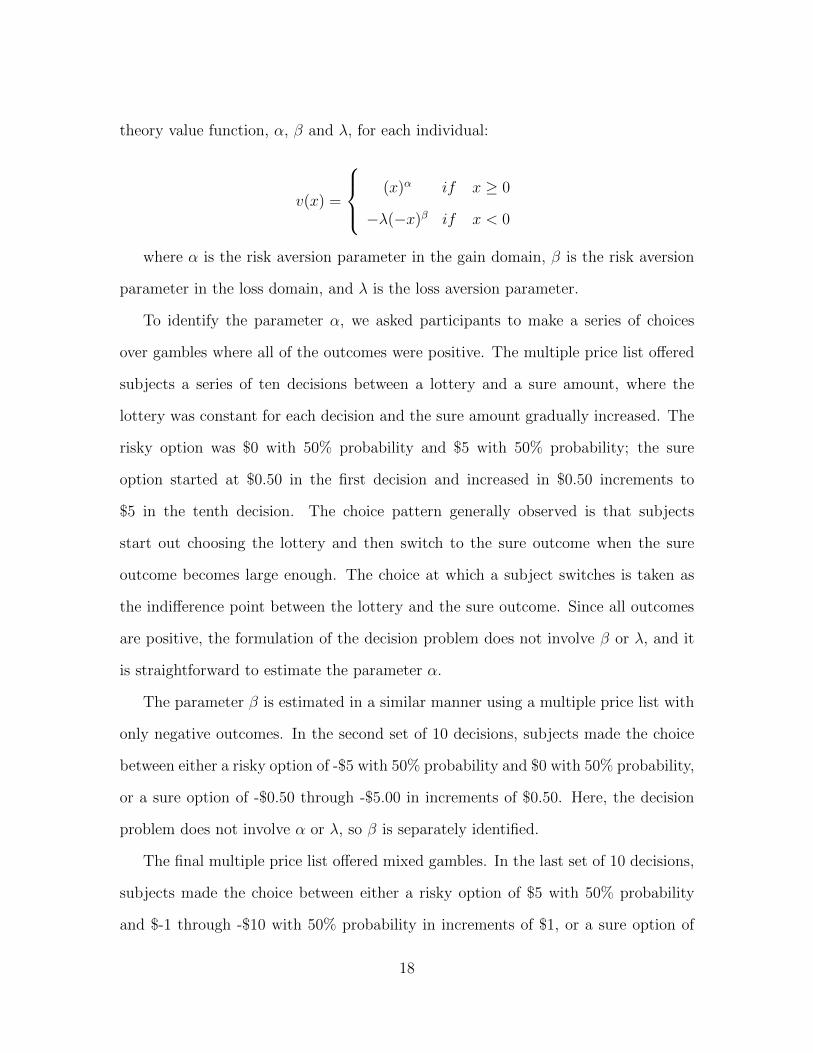
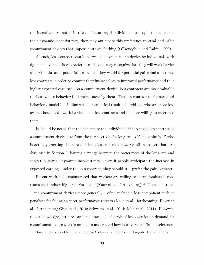
The results from Experiment 2 do not support the prediction of the standard

behavioral model. As shown in Figure 3, the maximum average WTP is higher for the

LOSS contract ($2.54, N = 41, SD = $1.73) than the GAIN contract ($1.76, N = 44,

SD = $1.48). This represents a statistically significant di↵erence between LOSS and

GAIN, which goes in the opposite direction than is predicted by the theory (Student’s

t-test 2-tailed p = 0.03, Wilcoxon-Mann-Whitney test of distribution p = 0.04).9

Because WTP is censored at $0 and $5, we also use a Tobit regression to confirm

our results. Regressing a treatment dummy (LOSS = 1, GAIN = 0) on WTP reveals

a similar result: the coe�cient on the dummy is 0.93 and is statistically significant

(p = 0.03).

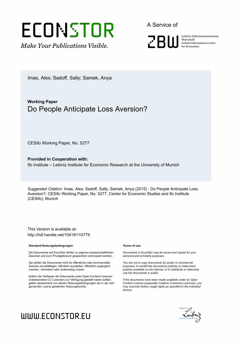
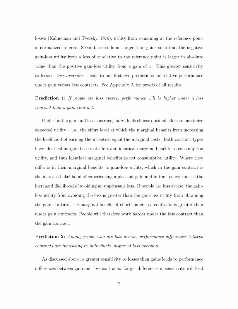
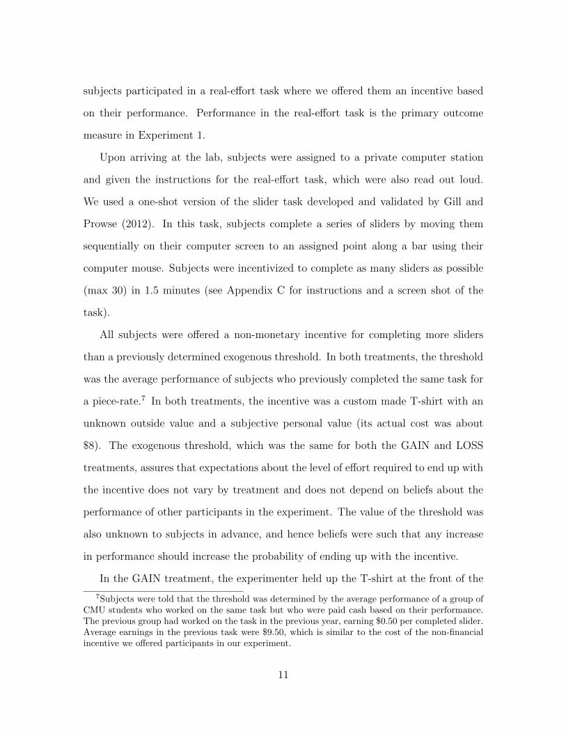
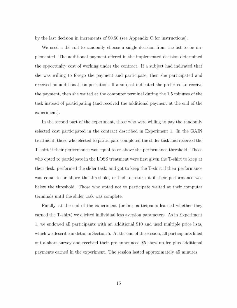
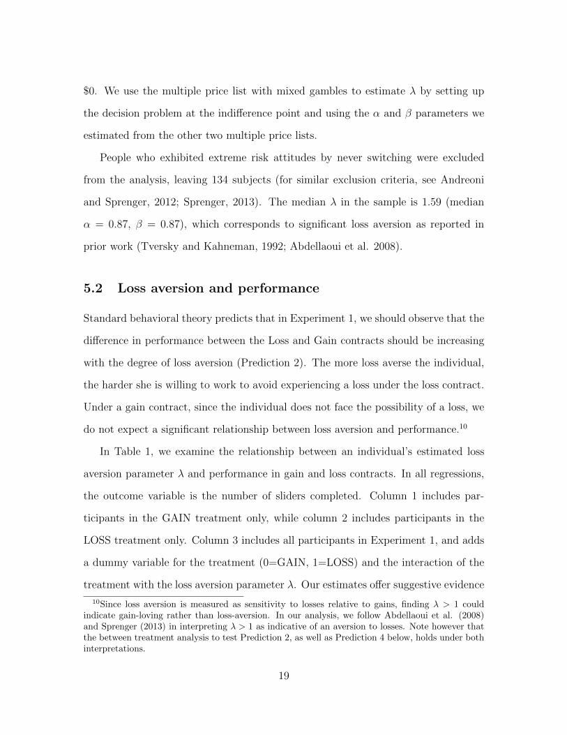
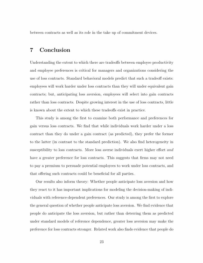
Figure 4 presents a histogram of maximum WTP by treatment. The majority

of participants in the GAIN treatment prefer to receive $1.00 (or less) rather than

work under a gain contract and less than 5% are willing to pay the maximum allowed

amount of $5. In contrast, nearly a third of participants in the LOSS treatment are

willing to pay at least $4 to work under a loss contract, with half of those willing to

9Out of 85 participants, 92% have consistent choices – i.e., once they choose to accept theadditional payment (rather than participate) they continue to do so for all higher values of thepayment. Dropping participants who are not consistent (5 subjects in LOSS and 2 in GAIN) doesnot a↵ect the results (p = 0.04 for the Student’s t-test and the Wilcoxon-Mann-Whitney test whencomparing LOSS and GAIN).

16

forgo $5 in order to participate. To test for di↵erences between the distributions, we

run the same non-parametric distribution test as in Experiment 1. The results show

that the distribution of WTP in the LOSS treatment is significantly to the right of

the distribution in the GAIN treatment (p = 0.03).

5 The e↵ect of loss aversion on performance and

contract preferences

Anticipation of loss aversion in our standard behavioral model predicts that WTP to

enter loss contracts should be lower than WTP to enter gain contracts, a hypothesis

that is rejected by our data. An alternative possibility, that people fail to antici-

pate loss aversion, predicts no di↵erence in WTP between the two contracts. This

alternative is also rejected by our data. Instead, we find that people do anticipate

loss aversion, but react to it in the opposite direction predicted by the standard be-

havioral model - people actually prefer the loss contract to the gain contract. What

mechanisms drive these results? To shed light on this question, we examine the

relationship between participants’ behavior and a separately-elicited individual loss

aversion parameter.

5.1 Construction of the loss aversion parameter

At the end of Experiments 1 and 2, we elicited individuals’ preferences over a series

of gambles using multiple price lists. Subjects received an additional $10 and made

a series of 30 binary decisions, choosing between sure payo↵s or risky payo↵s with

outcomes to be determined by a coin flip. Only one decision was randomly determined

to be paid out at the end of the experiment. Similar to Abdellaoui et al. (2008), the

set of 30 decisions allows us to separately estimate the three parameters of a prospect

17

theory value function, ↵, � and �, for each individual:

v(x) =

8><

>:

(x)↵ if x � 0

��(�x)� if x < 0

where ↵ is the risk aversion parameter in the gain domain, � is the risk aversion

parameter in the loss domain, and � is the loss aversion parameter.

To identify the parameter ↵, we asked participants to make a series of choices

over gambles where all of the outcomes were positive. The multiple price list o↵ered

subjects a series of ten decisions between a lottery and a sure amount, where the

lottery was constant for each decision and the sure amount gradually increased. The

risky option was $0 with 50% probability and $5 with 50% probability; the sure

option started at $0.50 in the first decision and increased in $0.50 increments to

$5 in the tenth decision. The choice pattern generally observed is that subjects

start out choosing the lottery and then switch to the sure outcome when the sure

outcome becomes large enough. The choice at which a subject switches is taken as

the indi↵erence point between the lottery and the sure outcome. Since all outcomes

are positive, the formulation of the decision problem does not involve � or �, and it

is straightforward to estimate the parameter ↵.

The parameter � is estimated in a similar manner using a multiple price list with

only negative outcomes. In the second set of 10 decisions, subjects made the choice

between either a risky option of -$5 with 50% probability and $0 with 50% probability,

or a sure option of -$0.50 through -$5.00 in increments of $0.50. Here, the decision

problem does not involve ↵ or �, so � is separately identified.

The final multiple price list o↵ered mixed gambles. In the last set of 10 decisions,

subjects made the choice between either a risky option of $5 with 50% probability

and $-1 through -$10 with 50% probability in increments of $1, or a sure option of

18

$0. We use the multiple price list with mixed gambles to estimate � by setting up

the decision problem at the indi↵erence point and using the ↵ and � parameters we

estimated from the other two multiple price lists.

People who exhibited extreme risk attitudes by never switching were excluded

from the analysis, leaving 134 subjects (for similar exclusion criteria, see Andreoni

and Sprenger, 2012; Sprenger, 2013). The median � in the sample is 1.59 (median

↵ = 0.87, � = 0.87), which corresponds to significant loss aversion as reported in

prior work (Tversky and Kahneman, 1992; Abdellaoui et al. 2008).

5.2 Loss aversion and performance

Standard behavioral theory predicts that in Experiment 1, we should observe that the

di↵erence in performance between the Loss and Gain contracts should be increasing

with the degree of loss aversion (Prediction 2). The more loss averse the individual,

the harder she is willing to work to avoid experiencing a loss under the loss contract.

Under a gain contract, since the individual does not face the possibility of a loss, we

do not expect a significant relationship between loss aversion and performance.10

In Table 1, we examine the relationship between an individual’s estimated loss

aversion parameter � and performance in gain and loss contracts. In all regressions,

the outcome variable is the number of sliders completed. Column 1 includes par-

ticipants in the GAIN treatment only, while column 2 includes participants in the

LOSS treatment only. Column 3 includes all participants in Experiment 1, and adds

a dummy variable for the treatment (0=GAIN, 1=LOSS) and the interaction of the

treatment with the loss aversion parameter �. Our estimates o↵er suggestive evidence

10Since loss aversion is measured as sensitivity to losses relative to gains, finding � > 1 couldindicate gain-loving rather than loss-aversion. In our analysis, we follow Abdellaoui et al. (2008)and Sprenger (2013) in interpreting � > 1 as indicative of an aversion to losses. Note however thatthe between treatment analysis to test Prediction 2, as well as Prediction 4 below, holds under bothinterpretations.

19

for Prediction 2. Loss aversion has no significant relationship with performance in the

GAIN treatment (p = 0.44). However, the coe�cient on � is positive and marginally

significant in the LOSS treatment (p = 0.06). The interaction term is also positive but

not significant at conventional levels (p = 0.13). These results o↵er suggestive sup-

port for the prediction of a di↵erential e↵ect of loss aversion on performance between

the two contract types.

5.3 Loss aversion and contract preferences

The standard behavioral theory predicts that in Experiment 2, if individuals antici-

pate loss aversion, we should observe larger treatment e↵ects on WTP among more

loss averse individuals (Prediction 4). Individuals who are more loss averse should be

willing to accept a smaller ‘additional payment’ instead of working under the LOSS

contract since the loss frame will hurt them most. That is, WTP to enter the loss

contract should be significantly decreasing in �, while we do not expect a significant

relationship between � and WTP to enter the gain contract.

Examining the relationship between loss aversion and preferences between con-

tracts in Experiment 2 does not support the prediction of the standard behavioral

theory; in fact, our results suggest the opposite pattern. We find that those who ex-

hibit greater loss aversion are willing to pay more to participate in the loss contract

than the gain contract. Table 2, which has the same structure as Table 1 except that

the dependent variable is WTP in Experiment 2, summarizes these results. Column

1 includes participants in the GAIN treatment only. Column 2 includes participants

in the LOSS treatment only. Column 3 includes all participants in Experiment 2

and adds a dummy variable for the treatment (0=GAIN, 1=LOSS) and the interac-

tion of the treatment with the loss aversion parameter �. The standard behavioral

20

model predicts a more negative � coe�cient in the LOSS treatment than the GAIN

treatment, and thus the interaction term should be negative. Our estimates do not

support these predictions. The coe�cient on � is small and not significant for partic-

ipants in the GAIN treatment. However, it is positive and marginally significant for

participants in the LOSS treatment (p = 0.07). The interaction term is also positive

and marginally significant (p = 0.07). Rather than avoiding loss contracts, our results

suggest that more loss averse individuals are more likely to select into them.

6 Interpretation

Our results demonstrate that, as predicted, individuals do exert higher e↵ort under

loss contracts; but in contrast to the theory, they prefer loss contracts to gain con-

tracts. Further, we find evidence that those who are most sensitive to losses are also

the ones who are most likely to select into loss contracts. That is, the most loss

averse individuals both work harder and have the highest WTP for loss contracts. As

discussed in Section 2, the greater the upward distortion in e↵ort under loss contracts

(relative to gain contracts), the larger are the utility costs experienced under loss

contracts. Why then would people want to enter a contract that induces them to

work ‘too hard’ by imposing the pain of potential losses?

We suggest that one possible mechanism driving our results is that individuals se-

lect into loss contracts as a commitment device. Models with dynamic inconsistency

in preferences have been used to explain suboptimal behavior in domains such as

savings and health (Laibson, 1997; O’Donoghue and Rabin, 1999). In the workplace,

dynamic inconsistency can take the following form. Individuals may enter into con-

tracts with a preference for working hard and earning a performance bonus, but when

it comes time to exert e↵ort, their preferences reverse: they shirk and fail to earn

21

the incentive. As noted in related literature, if individuals are sophisticated about

their dynamic inconsistency, they may anticipate this preference reversal and value

commitment devices that impose costs on shirking (O’Donoghue and Rabin, 1999).

As such, loss contracts can be viewed as a commitment device by individuals with

dynamically inconsistent preferences. People may recognize that they will work harder

under the threat of potential losses than they would for potential gains and select into

loss contracts in order to commit their future selves to improved performance and thus

higher expected earnings. As a commitment device, loss contracts are most valuable

to those whose behavior is distorted most by them. Thus, in contrast to the standard

behavioral model but in line with our empirical results, individuals who are more loss

averse should both work harder under loss contracts and be more willing to enter into

them.

It should be noted that the benefits to the individual of choosing a loss contract as

a commitment device are from the perspective of a long-run self, since the ‘self’ who

is actually exerting the e↵ort under a loss contract is worse o↵ in expectation. As

discussed in Section 2, barring a wedge between the preferences of the long-run and

short-run selves - dynamic inconsistency - even if people anticipate the increase in

expected earnings under the loss contract, they should still prefer the gain contract.

Recent work has demonstrated that workers are willing to enter dominated con-

tracts that induce higher performance (Kaur et al., forthcoming).11 These contracts

– and commitment devices more generally – often include a loss component such as

penalties for failing to meet performance targets (Kaur et al., forthcoming; Royer et

al., forthcoming; Gine et al., 2010; Schwartz et al., 2014; John et al., 2011). However,

to our knowledge, little research has examined the role of loss aversion in demand for

commitment. More work is needed to understand how loss aversion a↵ects preferences

11See also the work of Kaur et al. (2010), Cadena et al. (2011) and Augenblick et al. (2013).

22

between contracts as well as its role in the take up of commitment devices.

7 Conclusion

Understanding the extent to which there are tradeo↵s between employee productivity

and employee preferences is critical for managers and organizations considering the

use of loss contracts. Standard behavioral models predict that such a tradeo↵ exists:

employees will work harder under loss contracts than they will under equivalent gain

contracts; but, anticipating loss aversion, employees will select into gain contracts

rather than loss contracts. Despite growing interest in the use of loss contracts, little

is known about the extent to which these tradeo↵s exist in practice.

This study is among the first to examine both performance and preferences for

gain versus loss contracts. We find that while individuals work harder under a loss

contract than they do under a gain contract (as predicted), they prefer the former

to the latter (in contrast to the standard prediction). We also find heterogeneity in

susceptibility to loss contracts. More loss averse individuals exert higher e↵ort and

have a greater preference for loss contracts. This suggests that firms may not need

to pay a premium to persuade potential employees to work under loss contracts, and

that o↵ering such contracts could be beneficial for all parties.

Our results also inform theory: Whether people anticipate loss aversion and how

they react to it has important implications for modeling the decision-making of indi-

viduals with reference-dependent preferences. Our study is among the first to explore

the general question of whether people anticipate loss aversion. We find evidence that

people do anticipate the loss aversion, but rather than deterring them as predicted

under standard models of reference dependence, greater loss aversion may make the

preference for loss contracts stronger. Related work also finds evidence that people do

23

not anticipate loss aversion as predicted by standard behavioral models with rational

expectations. In the context of eliciting willingness to pay and willingness to accept

values for a mug, Loewenstein and Adler (1995) and Van Boven et al. (2000) find

evidence that prior to being endowed, subjects under-estimate their willingness to

accept.

Examining preferences and selection e↵ects is crucial for applying behavioral in-

sights in management and policy more broadly. For example, several studies find that

people are reluctant to realize losses on assets (Barberis, 2013). If this is the case,

whether and how people anticipate such behavior is critical for understanding their

trading decisions. The anticipation of future preferences has been explored in other

areas, such as models of rational addiction (Becker and Murphy, 1988), projection

bias (Loewenstein et al., 2003) and time preferences (Laibson, 1997; O’Donoghue and

Rabin, 1999). These models allow us to evaluate the extent to which we can view

individuals’ decision-making as rational and the extent to which people may be mak-

ing optimization mistakes. Further studies in the lab and field can help shed light

on this important yet under-explored question in the context of reference dependent

preferences.

References

Abdellaoui, Mohammed, Han Bleichrodt, and Olivier L’Haridon. 2008. “A TractableMethod to Measure Utility and Loss Aversion under Prospect Theory.” Journal ofRisk and Uncertainty, 36(3): 245-66.

Anderson, Lisa R., Francis J. DiTraglia, and Je↵rey R. Gerlach. 2011. “Measuring Al-truism in a Public Goods Experiment: A comparison of U.S. and Czech Subjects.”Experimental Economics, 14(3): 426-37.

Andreoni, James and Charles Sprenger. 2012. “Risk Preferences are Not Time Pref-erences.” The American Economic Review, 102(7): 3357-3376.

24

Augenblick, Ned, Muriel Niederle, and Charles Sprenger. 2013. “Working Over Time:Dynamic Inconsistency in Real E↵ort Tasks.” NBER Working Paper 18734.

Barberis, Nicholas C. 2013. “Thirty Years of Prospect Theory in Economics: A Re-view and Assessment.” Journal of Economic Perspectives 27(1): 173-96.

Becker, Gary S., and Kevin M. Murphy. 1998. “A Theory of Rational Addiction.”Journal of Political Economy 96(4): 675.

Brooks, Richard R. W., Alexander Stremitzer, and Stephan Tontrup. 2012. “Fram-ing Contracts: Why Loss Framing Increases E↵ort.” Journal of Institutional andTheoretical Economics, 168(1): 62-82.

Camerer, Colin F., George Loewenstein and Matthew Rabin, eds. 2004. Advances inBehavioral Economics, Princeton, NJ: Princeton University Press.

Charness, Gary, Uri Gneezy, and Alex Imas. 2013. “Experimental Methods: ElicitingRisk Preferences.” Journal of Economic Behavior and Organization, 87: 43-51.

De Quidt, Jonathan. 2014. “Your Loss Is My Gain: A Recruitment Experiment withFramed Incentives.” Working paper.

Dellavigna, Stefano. 2009. “Psychology and Economics: Evidence from the Field.”Journal of Economic Literature, 47(2): 315-72.

DiTraglia, Francis Joseph. “Experimental Public Goods in Prague and Williamsburg:An International Comparison.” 2006.

Ericson, Keith M. Marzilli, and Andreas Fuster. 2014. “The Endowment E↵ect.”Annual Review of Economics, 6(1): 555-79.

Fryer Jr, Roland G., Steven D. Levitt, John A. List, and Sally Sado↵, 2012. “Enhanc-ing the E�cacy of Teacher Incentives through Loss Aversion: A Field Experiment.”NBER Working paper 18237.

Gill, David, and Victoria Prowse. 2012. “A Structural Analysis of DisappointmentAversion in a Real E↵ort Competition.” American Economic Review 102(1): 469-503.

Gine, Xavier, Jessica Goldberg, Dan Silverman, and Dean Yang. 2012. “RevisingCommitments: Time Preference and Time-Inconsistency in the Field.” NBERWorking Paper 18065.

Holt, Charles A., and Susan K. Laury.2002. “Risk Aversion and Incentive E↵ects.”American Economic Review 92(5): 1644-655.

25

Hossain, Tanjim, and John A. List. 2012. “The Behavioralist Visits the Factory: In-creasing Productivity Using Simple Framing Manipulations.” Management Science58(12): 2151-167.

Imas, Alex. 2014. “Working for the ‘Warm Glow’: On the Benefits and Limits ofProsocial Incentives.” Journal of Public Economics, 114.

Kahneman, Daniel, and Amos Tversky. 1979.“Prospect Theory: An Analysis of De-cision under Risk.” Econometrica 47(2): 263.

Kahneman, Daniel, Jack L. Knetsch, and Richard H. Thaler. 1990. “Experimen-tal Tests of the Endowment E↵ect and the Coase Theorem.” Journal of PoliticalEconomy 98(6): 1325.

Kaur, Supreet, Michael Kremer, and Sendhil Mullainathan. 2010. “Self-Control andthe Development of Work Arrangements.” American Economic Review, Papers andProceedings, 100 (2): 624-628.

Kaur, Supreet, Michael Kremer, and Sendhil Mullainathan. “Self-control at Work.”Forthcoming, Journal of Political Economy

Koszegi, Botand, and Matthew Rabin. 2006. “A Model of Reference-Dependent Pref-erences.” The Quarterly Journal of Economics 121(4): 1133-165.

Laibson, David. 1997. “Golden Eggs and Hyperbolic Discounting.” The QuarterlyJournal of Economics, 112(2): 443-78.

Levitt, Steven D., John A. List, Susanne Neckermann and Sally Sado↵. 2012. “TheBehavioralist Goes to School: Leveraging Behavioral Economics to Improve Edu-cational Performance” NBER Working Paper 18165.

List, John A., and Anya Savikhin Samek. 2014. “The Behavioralist as Nutritionist:Leveraging Behavioral Economics To Improve Child Food Choice and Consump-tion.” Journal of Health Economics, 133-46.

Loewenstein, George, Ted O’Donoghue, and Matthew Rabin. 2003. “Projection Biasin Predicting Future Utility.” The Quarterly Journal of Economics, 118(4): 1209-248.

Loewenstein, George, and Daniel Adler. “A Bias in the Prediction of Tastes.” TheEconomic Journal, 105(431): 929.

Luft, Joan. 1994. “Bonus and Penalty Incentives Contract Choice by Employees.”Journal of Accounting and Economics 18(2): 181-206.

Madrian, Brigitte C. 2014. “Applying Insights from Behavioral Economics to PolicyDesign.” Annual Review of Economics, 6(1): 663-88.

26

O’Donoghue, Ted, and Matthew Rabin. 1999. “Doing It Now or Later.” AmericanEconomic Review 89(1): 103-24.

Royer, Heather, Mark F Stehr, and Justin R Sydnor. “Incentives, Commitments andHabit Formation in Exercise: Evidence from a Field Experiment with Workersat a Fortune-500 Company.”’ Forthcoming, American Economic Journal: AppliedEconomics

Samuelson, William, and Richard Zeckhauser. 1988. “Status Quo Bias in DecisionMaking.” Journal of Risk and Uncertainty, 1(1): 7-59.

Schmid, Friedrich, and Mark Trede. 1995. “A Distribution Free Test for the Two Sam-ple Problem for General Alternatives.” Computational Statistics and Data Analysis,20(4): 409-19.

Schwartz, J, Mochon, D., Wyper, L., Maroba, J., Patel, D., and Ariely, D. 2014.“Healthier by Precommitment.” Psychological Science, 25(2): 538-546.

Sprenger, Charles. 2013. “An Endowment E↵ect for Risk: Experimental Tests ofStochastic Reference Points,” Mimeo

Thaler, Richard H., and Eric J. Johnson. 1990. “Gambling with the House Moneyand Trying to Break Even: The E↵ects of Prior Outcomes on Risky Choice.”Management Science 36(6): 643-60.

Tversky, Amos, and Daniel Kahneman. 1992.“Advances in Prospect Theory: Cu-mulative Representation of Uncertainty.” Journal of Risk and Uncertainty, 5(4):297-323.

Van Boven, L., D. Dunning, and G. Loewenstein. 2000.“ Egocentric Empathy Gapsbetween Owners and Buyers: Misperceptions of the Endowment E↵ect.” Journalof Personality and Social Psychology, 79 (1): 66-76.

27

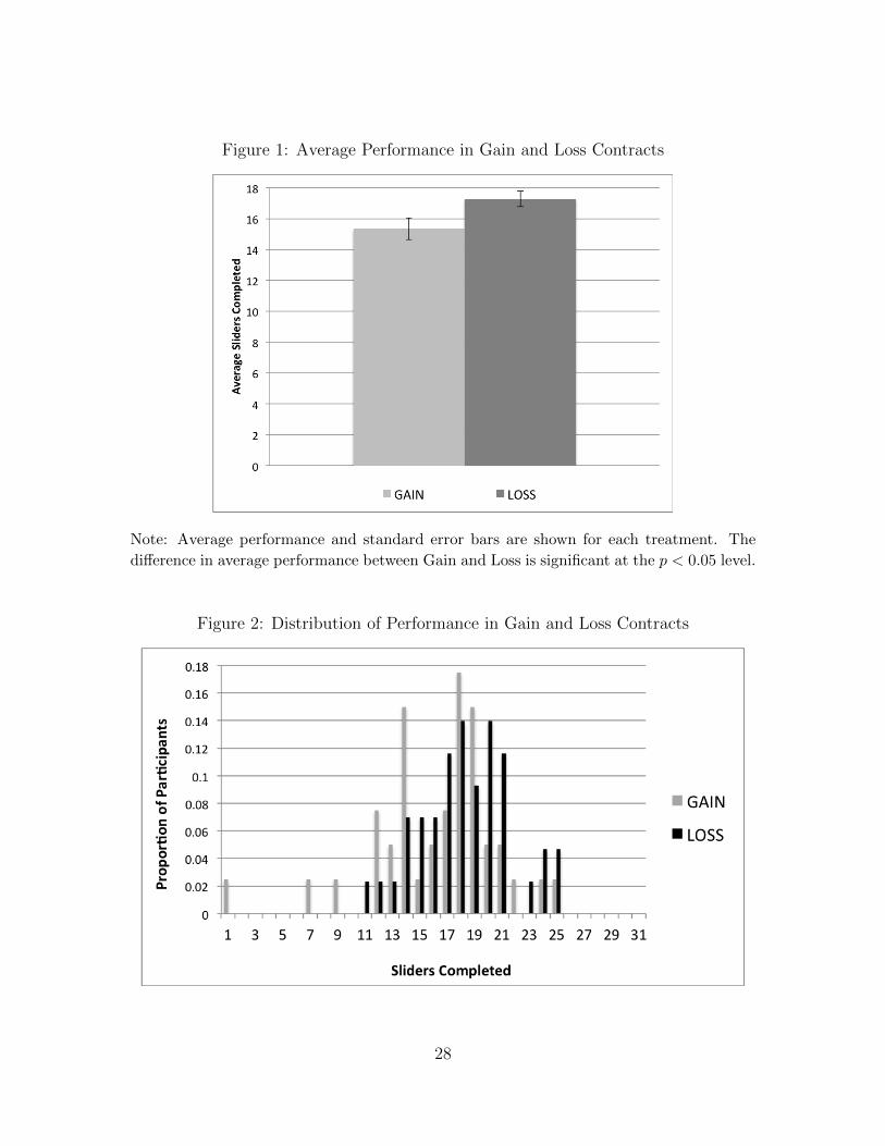
Figure 1: Average Performance in Gain and Loss Contracts

Note: Average performance and standard error bars are shown for each treatment. The

di↵erence in average performance between Gain and Loss is significant at the p < 0.05 level.

Figure 2: Distribution of Performance in Gain and Loss Contracts

28

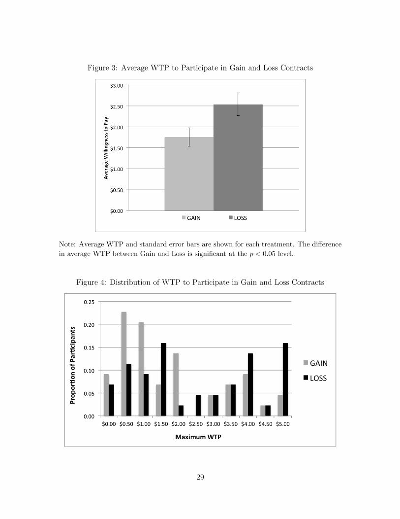
Figure 3: Average WTP to Participate in Gain and Loss Contracts

Note: Average WTP and standard error bars are shown for each treatment. The di↵erence

in average WTP between Gain and Loss is significant at the p < 0.05 level.

Figure 4: Distribution of WTP to Participate in Gain and Loss Contracts

29

A Proofs of Theoretical Predictions

To formalize the intuition discussed above, consider a representative agent whose

utility V is given by:

V = V (e, b, r) = e[u(b) + v(b|r)] + [1� e]v(0|r)� c(e)

where an individual receives a payo↵ b > 0 with probability equal to e↵ort e 2 (0, 1)

and receives 0 with probability 1�e; u(·) corresponds to standard consumption utility

over the payo↵, v(·|r) is the gain-loss prospect theory value function and c(·) is the

cost of e↵ort e that an individual exerts to obtain the bonus.12 Let u be an increasing

and concave function of b, and c be an increasing and convex function of e. Normalize

u(0) = 0. We define the utility derived in relation to a reference point r as follows

v(x|r) =

8><

>:

(x� r)↵ if x � r

�(x� r)� if x < r

where � > 1 is the loss aversion parameter and we assume ↵ = �.13 An individual

chooses optimal e↵ort e⇤ to maximize overall utility V :

maxe

V (e, b, r) = maxe

e[u(b) + v(b|r)] + [1� e]v(0|r)� c(e)

Taking the status quo model of prospect theory, when working under the gain contract

(r = 0), optimal e↵ort in the gain contract e

⇤G satisfies the following first order

condition:

c

0(e⇤G) = u(b) + b

↵ (2)

12In practice, we measure e↵ort through performance, which we assume is increasing in e↵ort e.13Tversky and Kahneman (1992) estimate � = 2.25 and median ↵ = � = 0.88. As discussed in

Section 5, we estimate �, ↵ and � separately in our data and find similar support for our assumptions.

30

Under the loss contract (r = b), optimal e↵ort in the loss contract e

⇤L satisfies the

following first order condition:

c

0(e⇤L) = u(b) + �b

� (3)

The first order conditions lead to our first prediction:

Proof of Prediction 1 If people are loss averse, performance will be higher under

a loss contract than a gain contract.

Proof. Under the assumptions that costs c are convex, the left hand sides of equa-

tion (2) and equation (3) are increasing in e↵ort e. If � > 1, then the right-hand side of

equation (3) is greater than the right hand side of equation (2), u(b)+�b

�> u(b)+b

↵

(under the assumption that ↵ = �).14 Thus, optimal e↵ort in the loss contract will

be greater than optimal e↵ort in the gain contract e⇤L > e

⇤G. Under the assumption

that performance is an increasing function of e↵ort, performance will be higher under

the loss contract than the gain contract. If � = 1, optimal e↵ort and performance

will be the same in loss and gain contracts; if � > 1, e↵ort and performance will be

higher in loss contracts.

Note that by the same logic as Prediction 1, if � < 1, e↵ort and performance will

be lower in loss contracts than gain contracts.

Proof of Prediction 2 Among people who are loss averse, performance di↵er-

ences between contracts are increasing in individuals’ degree of loss aversion.

Proof. As discussed above, among people who are loss averse, greater optimal e↵ort

under loss contracts versus gain contracts is due to greater sensitivity to losses than

gains � > 1. The di↵erence in optimal e↵ort e

⇤L � e

⇤G is increasing in the di↵erence

14This result does not require that ↵ = �. It is su�cient that � > b↵

b� .

31

in gain-loss utility � (under the assumption that e↵ort costs are convex). That is,

the more loss averse someone is, the harder she will work to avoid losses relative to

working for gains. Given the assumption that performance is an increasing function of

e↵ort, performance di↵erences between loss and gain contracts will be higher among

more loss averse people compared to less loss averse people.

Note that among people for whom � < 1, e↵ort and performance are higher under

gain contracts and this di↵erence increases as � decreases. That is, if a person is

less sensitive to losses than she is to gains, performance will be higher under gain

contracts and the gain-loss gap will increase as loss sensitivity decreases.

We now consider the participation constraint in which individuals are o↵ered a

choice between a certain amount w � 0 or the chance to participate in the task and

earn the uncertain payo↵ b. An individual will participate if V (e⇤, b, r) � u(w) +

w

↵, where V (e⇤, b, r) is the agent’s utility under optimal e↵ort e

⇤. Note as argued

and demonstrated by Kahneman, Knetsch and Thaler (1990), individuals choosing

between goods without being endowed with either behave as if their reference point

was the status quo. We follow this assumption when outlining the decision problem

between a certain payo↵ and the contract.

The greatest amount the agent would be willing to forgo in order to participate

(i.e., maximum willingness to pay) in the gain contract wG solves the following:

u(wG) + w

↵G = V (e⇤G, b, 0) (4)

where e

⇤G is optimal e↵ort under the gain contract as defined in equation (2).

Assuming that the agent has rational expectations over her preferences under

the loss contract, her maximum willingness to pay (WTP) to participate in the loss

32

contract wL solves the following:

u(wL) + w

↵L = V (e⇤L, b, b) (5)

where e

⇤L is optimal e↵ort under the loss contract as defined by equation (3).

Proof of Prediction 3 If people have dynamically consistent preferences and

rational expectations, willingness to pay for the gain contract will be higher than will-

ingness to pay for the loss contract, wG > wL.

Proof. Subtracting equation (5) from equation (4) gives:

[u(wG) + w

↵G]� [u(wL) + w

↵L] = V (e⇤G, b, 0)� V (e⇤L, b, b) (6)

We will show that the right hand side is positive which implies that wG > wL under

the assumption that u is increasing. Expanding terms

V (e⇤G, b, 0)� V (e⇤L, b, b) =⇣e

⇤G[u(b) + b

↵]� c(e⇤G)⌘�

⇣e

⇤Lu(b) + [1� e

⇤L]�(�b

�)� c(e⇤L)⌘

=⇣[e⇤Gu(b)� c(e⇤G)]� [e⇤Lu(b)� c(e⇤L)]

⌘+⇣e

⇤Gb

↵ + [1� e

⇤L]�b

�⌘

(7)

We first consider the term e

⇤Gb

↵ + [1 � e

⇤L]�b

� from (7), which is the di↵erence in

expected gain-loss utility under gain and loss contracts. From the assumptions that

e 2 (0, 1), b > 0 and � > 1, the term is positive15

e

⇤Gb

↵ + [1� e

⇤L]�b

�> 0 (8)

We next consider the term [e⇤Gu(b)� c(e⇤G)]� [e⇤Lu(b)� c(e⇤L)], which is the di↵erence

15Note that this result requires only reference dependent preferences and does not depend on thedegree of loss aversion as long as � > 0.

33

between gain and loss contracts in expected consumption utility net of costs. This

is Expected Utility from the standard framework where an agent chooses e↵ort to

maximize the following objective function:

maxe

e[u(b)]� c(e)

Optimal e↵ort under the standard framework e

⇤S satisfies the following first order

condition:

c

0(e⇤S) = u(b) (9)

The right-hand side of equation (9) is less than the right-hand side of equation (2)

(under the assumption that b > 0). Thus, e

⇤G > e

⇤S (under the assumption that

e↵ort costs are convex). From Prediction 1, if people are loss averse, then e

⇤L > e

⇤G.

Since e

⇤S optimizes equation (9), e⇤G and e

⇤L cannot be the optimal e↵ort – they are

too high. Because e

⇤L > e

⇤G, e

⇤L is further from the optimal e

⇤S than e

⇤G. Thus,

e

⇤Su(b)� c(e⇤S) > e

⇤Gu(b)� c(e⇤G) > e

⇤Lu(b)� c(e⇤L) and

[e⇤Gu(b)� c(e⇤G)]� [e⇤Lu(b)� c(e⇤L)] > 0 (10)

By equations (6), (7), (8) and (10), wG > wL. The maximum WTP for the gain

contract is higher than the maximum WTP for the loss contract.

Note that if people do not have rational expectations regarding their degree of

loss aversion, and in turn, the di↵erential e↵ect of the loss contract on behavior,

they will expect their reference point and optimal e↵ort under the loss contract to

be the same as it is under the gain contract. In this case, the maximum WTP for

the loss contract will be equal to maximum WTP for the gain contract, given by (4),

wL = wG = V (e⇤G, b, 0).

34

Our last prediction follows,

Proof of Prediction 4 If people are dynamically consistent and have rational

expectations, di↵erences in willingness to pay will be larger among people who are

more loss averse.

Proof. We will show that the right hand side of equation (6) is increasing in �. This

implies that the di↵erence in WTP for gain and loss contracts wG�wL is increasing in

loss aversion (under the assumptions that u is increasing and concave). Di↵erentiating

with respect to � gives

@

@�

�V (e⇤G, b, 0)� V (e⇤L, b, b)

�= �@e

⇤L

@�

u(b)� @e

⇤L

@�

�b

� + [1� e

⇤L]b

� +@c

@e

⇤L

@e

⇤L

@�

= [1� e

⇤L]b

� +@e

⇤L

@�

⇣@c

@e

⇤L

� [(u)b+ �b

�]⌘

= [1� e

⇤L]b

�

where the final equality follows from equation (3) which shows that c0(e⇤L) � [(u)b +

�b

�] = 0 evaluated at e

⇤L. The right hand side is positive [1 � e

⇤L]b

�> 0 under the

assumptions that e 2 (0, 1) and b > 0. Thus V (e⇤L, b, 0) � V (e⇤L, b, b) is increasing in

� which implies that the di↵erence in willingness to pay for gain and loss contracts

wG � wL is increasing in individuals’ degree of loss aversion.

35

B Description of pilot experiments

Below we describe the design and results of two pilot experiments conducted prior

to the experiments discussed in the main text. Pilot experiment 1 is analogous to

Experiment 1 (Section 3). Pilot experiment 2 is analogous to Experiment 2 (Section

4).

Pilot experiment 1: E↵ort under gain and loss contracts

Experimental design

Pilot experiment 1 was implemented among 62 participants at the University of Cal-

ifornia San Diego. Subjects were randomized at the session level to either a GAIN or

LOSS treatment and then participated in a one-shot task (sessions included 6 people

on average and lasted about 15 minutes).

Upon arriving in the lab, subjects were assigned to a computer station and given

the instructions, which were also read aloud. In both treatments, we first explained

the task students would perform and then o↵ered a performance-based incentive. For

the real-e↵ort task, we used the slider task discussed in Section 3. Subjects had 2

minutes to move up to 48 “sliders”.

All subjects were o↵ered an incentive for correctly completing more sliders than a

previously determined threshold. The threshold was set within each treatment such

that half of the participants in each group were expected to receive the incentive.16

In the GAIN treatment, subjects received the incentive if their performance on the

slider task was equal to or above the threshold. In the LOSS treatment, participants

16The threshold was determined by the average performance from a randomly chosen previoussession of the same treatment. Participants were informed of what constituted the threshold, butnot its value, prior to performing the e↵ort task. In the first session of each treatment, we used anaverage from a previous pilot study.

36

were endowed with the incentive before performing the slider task and were told they

would keep the incentive if their performance was equal to or above the threshold.

If their performance was below the threshold, participants in the LOSS treatment

had to return the incentive. This design created two payo↵-equivalent contracts: one

framed as a gain and the other framed as a loss (the intra-treatment threshold ensures

that earnings do not di↵er across treatments even if average e↵ort does).

In both treatments, the incentive was a custom made t-shirt with an unknown

outside value and a subjective personal value (its actual cost was about $8). In the

GAIN treatment, the experimenter held up the T-shirt at the front of the room and

told subjects they would receive it if their performance on the slider task was equal to

or above the threshold; otherwise they would receive nothing. In the LOSS treatment,

participants were given a T-shirt, which remained at their station throughout the

session. The experimenter told subjects that they would keep the T-shirt if their

performance was equal to or above the threshold; otherwise they would have to return

it. Subjects then performed the slider task for 2 minutes. After completing the task,

subjects filled out a short survey and received payment, including a show-up fee of

$5.

Results

Similar to the results of Experiment 1, the results in pilot experiment 1 support the

prediction of the standard behavioral model that performance will be higher in loss

contracts than gain contracts. Subjects in the GAIN treatment completed an average

of 11.88 sliders (N = 32, SD = 5.55) compared to an average in the LOSS treatment

of 15.27 sliders (N = 30, SD = 4.44). The 0.6 standard deviation di↵erence in

performance is statistically significant at the p < 0.01 level.

37

Pilot experiment 2: Anticipation of loss aversion and choicebetween contracts

Experimental design

In pilot experiment 2, we examine whether people anticipate loss aversion – that is,

whether they are more likely to select into a gain rather than a loss contract. To

do this, we elicited participants’ willingness to pay to participate in each of the two

incentive schemes used in pilot experiment 1.

Pliot experiment 2 was implemented among 60 participants at the University

of Wisconsin-Madison BRITE (Behavioral Research Insights through Experiments)

Laboratory. Using a between-subject design, we elicited willingness to pay to partic-

ipate in one of the two treatments described in pilot experiment 1: GAIN or LOSS.

As in pilot experiment 1, we randomized at the session level (sessions included 10

people on average and lasted about 40 minutes).

Upon arriving in the lab, subjects were assigned to a computer station and given

the instructions, which were also read aloud. The experiment proceeded in two parts.

In the first part, subjects were given 2 minutes to participate in the slider task for

no pay. In the second part, we elicited willingness to pay (WTP) to participate in

an incentivized version of the task. In the GAIN treatment, the experimenter held

up the T-shirt at the front of the room and read the instructions describing the gain

contract from pilot experiment 1. The LOSS treatment was identical except that the

experimenter read the instructions describing the loss contract from pilot experiment

1.

Subjects were then asked to indicate their maximum WTP out of their $10 show-

up fee to work under the o↵ered contract. We elicited WTP using a multiple price

list. In our paradigm, participants made a series of decisions between paying a price

38

and participating, or paying nothing and not participating. The decision to not

participate was constant (i.e., $0) while the price to participate increased from $0 to

$10 from the first decision to the last. We then used a die roll to randomly choose a

single decision from the list to be implemented. If a subject indicated she was willing

to pay the chosen cost, she participated and the cost was deducted from her show up

fee. If she indicated she was not willing to pay the chosen cost, she did not participate

and nothing was deducted from her show up fee.

In the GAIN treatment, those who paid to participate completed the slider task

and received the T-shirt if their performance was above average. Participating sub-

jects in the LOSS treatment were first given the T-shirt, then performed the slider

task, and either got to keep the T-shirt or had to return it, again depending on their

performance. At the end of the session, all participants filled out a short survey and

received payment.

Results

Similar to Experiment 2, the results from pilot study 2 do not support the prediction

of the standard behavioral model that WTP will be higher for the gain contract than

the loss contract. As in Experiment 2, average WTP in Pilot study 2 was higher for

the LOSS contract ($2.58, N=30, SD=$1.97) than the GAIN contract ($2.17, N=30,

SD=$2.14).17 Overall, we find no evidence that people prefer GAIN to LOSS.

17One participant in the gain treatment reported inconsistent WTP across the multiple price list.The results reported above use the subject’s first switching point (i.e., lowest WTP). Dropping theparticipant from the analysis decreases average WTP in the gain treatment to $2.14.

39

C Instructions for Experiment 1 and 2

Instructions for all treatments

Welcome to our short experiment. You will get a $5 show up fee just for coming in

today.

Please pay attention to the instructions carefully. You will be asked several ques-

tions throughout the study to make sure that you are reading and understanding the

instructions. You will NOT get paid if you do not follow all instructions carefully.

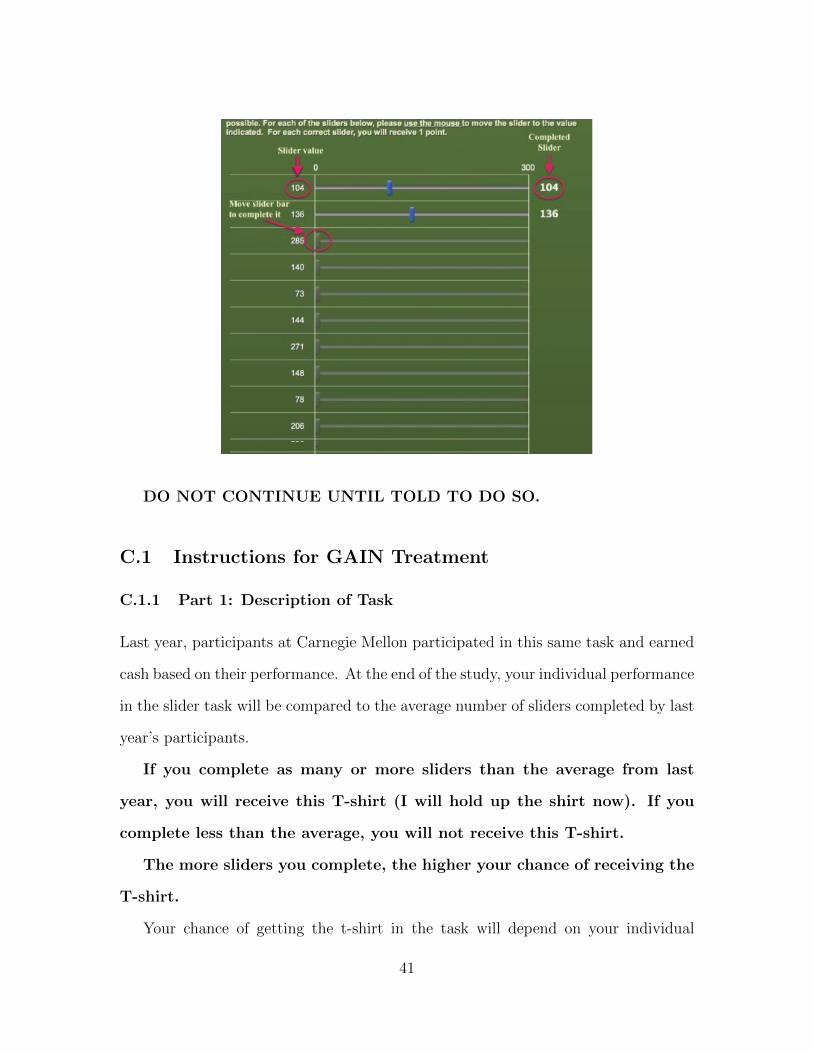
Today you will perform a slider task.

In this task, you will see a screen with 30 sliders on it. In this part you will have

1.5 minutes (90 seconds) to move as many sliders as you can to the value indicated.

Each slider you move to the value indicated is considered completed and earns you 1

point. You should only use your mouse to move sliders by clicking and dragging on

the slider – using the keyboard is not allowed. You should try to complete as many

sliders as you can.

The picture below shows you the slider task. The value that you need to move

each slider to appears to the left of the slider. Dragging the slider changes the value

on the right. Match the value on the right to the one on the left to complete the

slider. You can complete sliders in any order you like

40

DO NOT CONTINUE UNTIL TOLD TO DO SO.

C.1 Instructions for GAIN Treatment

C.1.1 Part 1: Description of Task

Last year, participants at Carnegie Mellon participated in this same task and earned

cash based on their performance. At the end of the study, your individual performance

in the slider task will be compared to the average number of sliders completed by last

year’s participants.

If you complete as many or more sliders than the average from last

year, you will receive this T-shirt (I will hold up the shirt now). If you

complete less than the average, you will not receive this T-shirt.

The more sliders you complete, the higher your chance of receiving the

T-shirt.

Your chance of getting the t-shirt in the task will depend on your individual

41

performance relative to last year’s average. It does not depend on the performance

of anyone else in this room.

[EXPERIMENT 2 ONLY - PARTICIPANTS COMPLETE ELICITATION OF

WILLLINGNESS TO PAY (SECTION C.3.1)]

C.1.2 Part 2: Performance of Task

Slider Task Instructions

C.1.3 Part 1: Description of Task

You will now perform the slider task. If you complete as many or more sliders

than last years average, you will get the T-shirt as a bonus. If you complete

fewer sliders than last year’s average, you will not get the T-shirt.

The more sliders you complete, the higher your chance of getting the

T-shirt.

Welcome to the Slider Task. You have 90 seconds to complete as many of the

sliders as possible. For each of the sliders below, please use the mouse to move the

slider to the value indicated. For each correct slider, you will receive 1 point.

C.2 Instructions for LOSS Treatment

You will receive a t-shirt for performing the slider task (I will hold up the

T-shirt now).

Last year, participants at Carnegie Mellon participated in this same task and

earned cash based on their performance. At the end of the study, your individual

performance in the slider task will be compared to the average number of sliders

completed by last year’s participants.

42

If you complete as many or more sliders than the average from last

year, you will keep your T-shirt. If you complete fewer sliders than the

average, you will give up your T-shirt.

The more sliders you complete, the higher your chance of keeping your

T-shirt.

Your chance of keeping your t-shirt in the task will depend on your individual

performance relative to last years average. It does not depend on the performance of

anyone else in this room.

[EXPERIMENT 2 ONLY - PARTICIPANTS COMPLETE ELICITATION OF

WILLLINGNESS TO PAY (SECTION C.3.2)]

C.2.1 Part 2: Performance of Task

Slider Task Instructions

PLEASE WAIT TO RECEIVE YOUR T-SHIRT FOR THE TASK

You will now perform the slider task. You were given a T-shirt to carry out this

task. If you complete as many or more sliders than last year’s average,

you will keep your T-shirt. If you complete fewer sliders than last year’s

average, you will lose your T-shirt.

The more sliders you complete, the higher your chance of keeping your

T-shirt and not losing it.

Welcome to the Slider Task. You have 90 seconds to complete as many of the

sliders as possible. For each of the sliders below, please use the mouse to move the

slider to the value indicated. For each correct slider, you will receive 1 point.

43

C.3 Elicitation of Willingness to Pay (WTP)

C.3.1 Instructions for GAIN Treatment

Do you want to participate?

In this part, you will make a series of decisions. In each line, you will decide either

to participate in the slider task, or to get an additional amount of money between

$0 and $10. After you are done making your decisions, we will roll a die to be the

‘choice that counts.’

If you decide to participate in the slider task in the choice that counts, then: You

will perform the slider task. If you complete as many or more sliders than

last years average, you will receive the T-shirt.

If you decide to get the additional amount of money in the ‘choice that counts,’

then: You will wait quietly for 1.5 minutes and will not participate in the

task You will not have a chance to receive the T-shirt.

You will not know which choice is the ‘choice that counts’ until after you have

made your decisions. Because we are making a random draw, any of the choices could

be the ‘choice that counts.’ Therefore, you should think carefully about the choice

you make on each line. The more often you answer “YES”, the greater your chances

of participating in part 2.

Here is an example. Look at question 4 below. Suppose question 4 is chosen as

the ‘choice that counts.’ If you said “YES” in question 4, you would participate in

the slider task for a chance to get the T-shirt but receive no additional amount of

money. If you said “NO” in question 4, you would receive a $1.50 additional amount

of money but would not participate in the slider task.

If the additional payment is $1.50, do you want to participate in the slider task?

a. Yes, I want to participate and have the opportunity of receiving the T-shirt. b.

44

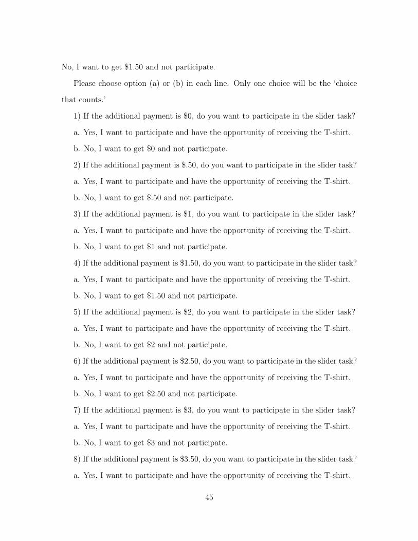
No, I want to get $1.50 and not participate.

Please choose option (a) or (b) in each line. Only one choice will be the ‘choice

that counts.’

1) If the additional payment is $0, do you want to participate in the slider task?

a. Yes, I want to participate and have the opportunity of receiving the T-shirt.

b. No, I want to get $0 and not participate.

2) If the additional payment is $.50, do you want to participate in the slider task?

a. Yes, I want to participate and have the opportunity of receiving the T-shirt.

b. No, I want to get $.50 and not participate.

3) If the additional payment is $1, do you want to participate in the slider task?

a. Yes, I want to participate and have the opportunity of receiving the T-shirt.

b. No, I want to get $1 and not participate.

4) If the additional payment is $1.50, do you want to participate in the slider task?

a. Yes, I want to participate and have the opportunity of receiving the T-shirt.

b. No, I want to get $1.50 and not participate.

5) If the additional payment is $2, do you want to participate in the slider task?

a. Yes, I want to participate and have the opportunity of receiving the T-shirt.

b. No, I want to get $2 and not participate.

6) If the additional payment is $2.50, do you want to participate in the slider task?

a. Yes, I want to participate and have the opportunity of receiving the T-shirt.

b. No, I want to get $2.50 and not participate.

7) If the additional payment is $3, do you want to participate in the slider task?

a. Yes, I want to participate and have the opportunity of receiving the T-shirt.

b. No, I want to get $3 and not participate.

8) If the additional payment is $3.50, do you want to participate in the slider task?

a. Yes, I want to participate and have the opportunity of receiving the T-shirt.

45

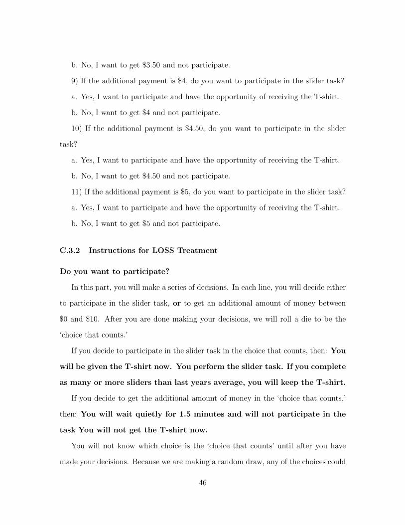
b. No, I want to get $3.50 and not participate.

9) If the additional payment is $4, do you want to participate in the slider task?

a. Yes, I want to participate and have the opportunity of receiving the T-shirt.

b. No, I want to get $4 and not participate.

10) If the additional payment is $4.50, do you want to participate in the slider

task?

a. Yes, I want to participate and have the opportunity of receiving the T-shirt.

b. No, I want to get $4.50 and not participate.

11) If the additional payment is $5, do you want to participate in the slider task?

a. Yes, I want to participate and have the opportunity of receiving the T-shirt.

b. No, I want to get $5 and not participate.

C.3.2 Instructions for LOSS Treatment

Do you want to participate?

In this part, you will make a series of decisions. In each line, you will decide either

to participate in the slider task, or to get an additional amount of money between

$0 and $10. After you are done making your decisions, we will roll a die to be the

‘choice that counts.’

If you decide to participate in the slider task in the choice that counts, then: You

will be given the T-shirt now. You perform the slider task. If you complete

as many or more sliders than last years average, you will keep the T-shirt.

If you decide to get the additional amount of money in the ‘choice that counts,’

then: You will wait quietly for 1.5 minutes and will not participate in the

task You will not get the T-shirt now.

You will not know which choice is the ‘choice that counts’ until after you have

made your decisions. Because we are making a random draw, any of the choices could

46

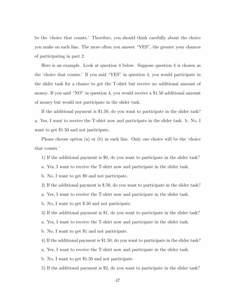
be the ‘choice that counts.’ Therefore, you should think carefully about the choice

you make on each line. The more often you answer “YES”, the greater your chances

of participating in part 2.

Here is an example. Look at question 4 below. Suppose question 4 is chosen as

the ‘choice that counts.’ If you said “YES” in question 4, you would participate in

the slider task for a chance to get the T-shirt but receive no additional amount of

money. If you said “NO” in question 4, you would receive a $1.50 additional amount

of money but would not participate in the slider task.

If the additional payment is $1.50, do you want to participate in the slider task?

a. Yes, I want to receive the T-shirt now and participate in the slider task. b. No, I

want to get $1.50 and not participate.

Please choose option (a) or (b) in each line. Only one choice will be the ‘choice

that counts.’

1) If the additional payment is $0, do you want to participate in the slider task?

a. Yes, I want to receive the T-shirt now and participate in the slider task.

b. No, I want to get $0 and not participate.

2) If the additional payment is $.50, do you want to participate in the slider task?

a. Yes, I want to receive the T-shirt now and participate in the slider task.

b. No, I want to get $.50 and not participate.

3) If the additional payment is $1, do you want to participate in the slider task?

a. Yes, I want to receive the T-shirt now and participate in the slider task.

b. No, I want to get $1 and not participate.

4) If the additional payment is $1.50, do you want to participate in the slider task?

a. Yes, I want to receive the T-shirt now and participate in the slider task.

b. No, I want to get $1.50 and not participate.

5) If the additional payment is $2, do you want to participate in the slider task?

47

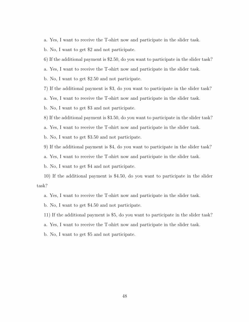
a. Yes, I want to receive the T-shirt now and participate in the slider task.

b. No, I want to get $2 and not participate.

6) If the additional payment is $2.50, do you want to participate in the slider task?

a. Yes, I want to receive the T-shirt now and participate in the slider task.

b. No, I want to get $2.50 and not participate.

7) If the additional payment is $3, do you want to participate in the slider task?

a. Yes, I want to receive the T-shirt now and participate in the slider task.

b. No, I want to get $3 and not participate.

8) If the additional payment is $3.50, do you want to participate in the slider task?

a. Yes, I want to receive the T-shirt now and participate in the slider task.

b. No, I want to get $3.50 and not participate.

9) If the additional payment is $4, do you want to participate in the slider task?

a. Yes, I want to receive the T-shirt now and participate in the slider task.

b. No, I want to get $4 and not participate.

10) If the additional payment is $4.50, do you want to participate in the slider

task?

a. Yes, I want to receive the T-shirt now and participate in the slider task.

b. No, I want to get $4.50 and not participate.

11) If the additional payment is $5, do you want to participate in the slider task?

a. Yes, I want to receive the T-shirt now and participate in the slider task.

b. No, I want to get $5 and not participate.

48