Seediscussions,stats,andauthorprofilesforthispublicationat:https://www.researchgate.net/publication/238620918

Steady-stateSolutionofFixed-speedWindTurbinesFollowingFaultConditionsThroughExtrapolationtotheLimitCycle

ARTICLEinIETEJOURNALOFRESEARCH·JANUARY2011

ImpactFactor:0.19·DOI:10.4103/0377-2063.78297

CITATIONS

2

READS

15

4AUTHORS,INCLUDING:

RafaelPeña

UniversidadAutónomadeSanLuisPotosí

22PUBLICATIONS33CITATIONS

SEEPROFILE

Availablefrom:RafaelPeña

Retrievedon:18February2016

12 IETE JOURNAL OF RESEARCH | VOL 57 | ISSUE 1 | JAN-FEB 2011

Steady-state Solution of Fixed-speed Wind Turbines Following Fault Conditions Through Extrapolation to

the Limit CycleRafael Peña, Aurelio Medina and Olimpo Anaya-Lara1

División de Estudios de Posgrado, Facultad de Ingeniería Eléctrica, Universidad Michoacana de San Nicolás de Hidalgo, Edificio de la División de Estudios de Posgrado de la Facultad de Ingeniería Eléctrica, Ciudad Universitaria,

Francisco J. Mújica S/N, CP: 58030, Morelia, Michoacán, México, 1Institute for Energy and Environment, University of Strathclyde, 204 George Street, Glasgow, G1 1XW, United Kingdom

ABSTRACT

A methodology to efficiently calculate the steady-state solution of fixed-speed induction generator (FSIG) based wind turbines, using a Newton algorithm and a Numerical Differentiation (ND) process for the extrapolation to the limit cycle is presented. This approach can be extremely useful in the development of steady-state studies of modern large-scale power systems with significant share of wind power based on FSIGs. A conventional Brute Force (BF) procedure is applied for comparison purposes to demonstrate the efficiency of the proposed methodology. The study involves the starting sequence of wind turbines and also the transient behavior of a single wind turbine after a disturbance. The simulations are conducted using a modeling platform developed by the authors to analyze power networks with high penetration of renewable sources.

Keywords:Brute force, Limit cycle, Numerical differentiation, Simulations, Steady state, Wind turbines.

1. INTRODUCTION

In order to analyze the steady-state and dynamic behavior of wind farms and their interaction with the network, it has become increasingly important to have suitable wind turbine models which can be easily integrated into power systems simulation software. There are several models available in the open literature, which may differ significantly in terms of the level of modeling detail and data requirements, depending on the particular aims of the study and the wind turbine technology under consideration [1-5].

The generator most widely used in both fixed-speed and variable-speed wind energy systems is the induction generator [6]. To simplify the analysis and to reduce the computational simulation effort, the generator is typically represented in the dq reference frame [7-9], and some models have been developed in state-space form to facilitate control design [10].

A direct integration of the state variables can be used to get the steady-state solution of a fixed-speed induction generator (FSIG) following a disturbance; this repetitive process, known as Brute Force (BF), is applied until the initial transient dies out. However, convergence difficulties and a considerable computational effort can be two important disadvantages of the BF technique.

Hence, in order to reach the steady state in a more efficient way, the use of a Newton method for the extrapolation to the limit cycle based on a Numerical Differentiation (ND) [11] procedure is described. It can be applied for the analysis of large-scale power systems which contain nonlinear and time-varying components, thus avoiding the considerably long periods of time that may be needed by a conventional time-domain solution based on the repetitive application of a numerical integration method [12-14].

The proposed methodology may be very useful in studies where the time period of interest is the steady state, such as in harmonic, contingency analysis and risk assessment of networks with high penetration of wind power. The concept is illustrated with two case studies: with a single wind turbine connected to an infinite bus and with a 15-turbine wind farm. A modeling platform developed by the authors was used to conduct the studies.

2. MODEL OF A FIXED-SPEED WIND TURBINE

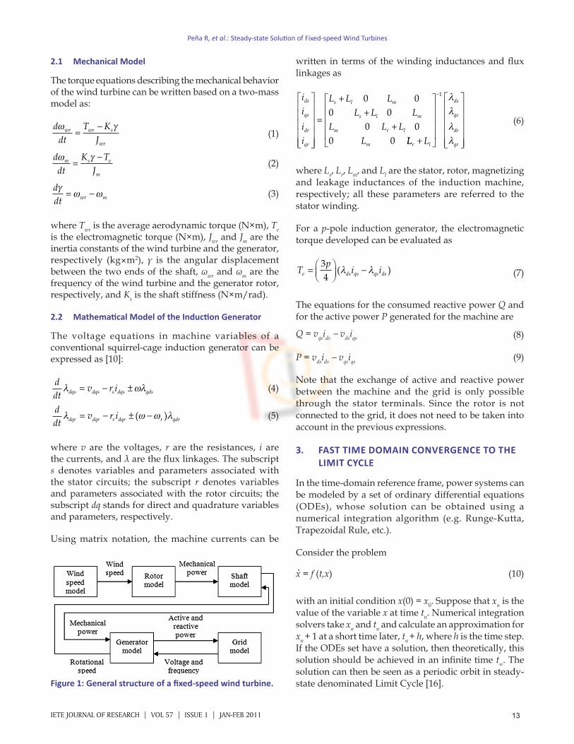
Figure 1 shows the general structure of a fixed-speed wind turbine model [15]. Due to relevance to the proposed methodology, only the mechanical model of the turbine and the mathematical model of the squirrel-cage induction generator are discussed in more detail.

13IETE JOURNAL OF RESEARCH | VOL 57 | ISSUE 1 | JAN-FEB 2011

2.1 Mechanical Model

The torque equations describing the mechanical behavior of the wind turbine can be written based on a two-mass model as:

ddt

T KJ

wr wr s

wr

ω γ=

−

(1)

ddt

K TJ

m s e

m

ω γ=

−

(2)

ddt wr mγ

ω ω= −

(3)

where Twr is the average aerodynamic torque (N×m), Te is the electromagnetic torque (N×m), Jwr and Jm are the inertia constants of the wind turbine and the generator, respectively (kg×m2), γ is the angular displacement between the two ends of the shaft, ωwr and ωm are the frequency of the wind turbine and the generator rotor, respectively, and Ks is the shaft stiffness (N×m/rad).

2.2 Mathematical Model of the Induction Generator

The voltage equations in machine variables of a conventional squirrel-cage induction generator can be expressed as [10]:

ddt

v r idqs dqs s dqs qdsλ ωλ= − ±

(4)

ddt

v r idqr dqr r dqr r qdrλ ω ω λ= − ± −( )

(5)

where v are the voltages, r are the resistances, i are the currents, and λ are the flux linkages. The subscript s denotes variables and parameters associated with the stator circuits; the subscript r denotes variables and parameters associated with the rotor circuits; the subscript dq stands for direct and quadrature variables and parameters, respectively.

Using matrix notation, the machine currents can be

written in terms of the winding inductances and flux linkages as

iiii

L L LL L L

L L LL

ds

qs

dr

qr

s l m

s l m

m r l

m

=

++

+

0 00 0

0 00 0 LL Lr l

ds

qs

dr

qr+

−1

(6)

where Ls, Lr, Lm, and Ll are the stator, rotor, magnetizing and leakage inductances of the induction machine, respectively; all these parameters are referred to the stator winding.

For a p-pole induction generator, the electromagnetic torque developed can be evaluated as

Tp

i ie ds qs qs ds=

−34( )

(7)

The equations for the consumed reactive power Q and for the active power P generated for the machine are

Q = vqsids - vdsiqs (8)

P = vdsids - vqsiqs (9)

Note that the exchange of active and reactive power between the machine and the grid is only possible through the stator terminals. Since the rotor is not connected to the grid, it does not need to be taken into account in the previous expressions.

3. FAST TIME DOMAIN CONVERGENCE TO THE LIMIT CYCLE

In the time-domain reference frame, power systems can be modeled by a set of ordinary differential equations (ODEs), whose solution can be obtained using a numerical integration algorithm (e.g. Runge-Kutta, Trapezoidal Rule, etc.).

Consider the problem .x = f (t,x) (10)

with an initial condition x(0) = x0. Suppose that xn is the value of the variable x at time tn. Numerical integration solvers take xn and tn and calculate an approximation for xn + 1 at a short time later, tn + h, where h is the time step. If the ODEs set have a solution, then theoretically, this solution should be achieved in an infinite time t∞. The solution can then be seen as a periodic orbit in steady-state denominated Limit Cycle [16].Figure 1: General structure of a fixed-speed wind turbine.

Peña R, et al.: Steady-state Solution of Fixed-speed Wind Turbines

14 IETE JOURNAL OF RESEARCH | VOL 57 | ISSUE 1 | JAN-FEB 2011

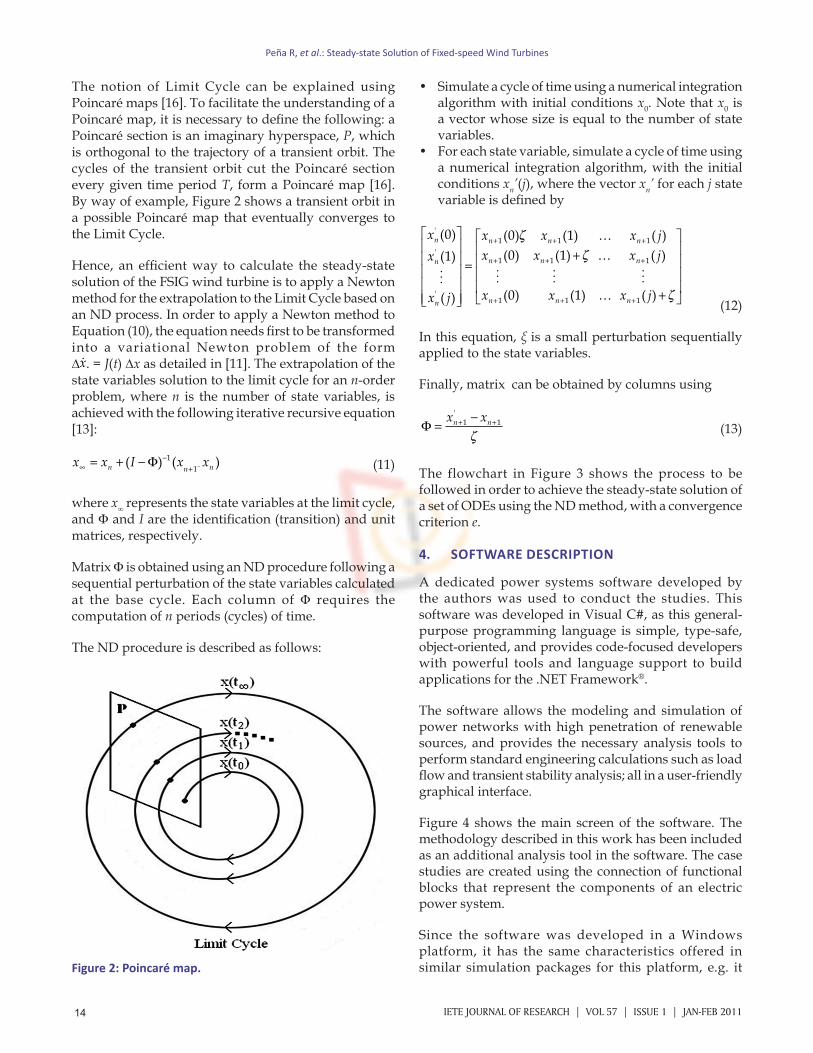
The notion of Limit Cycle can be explained using Poincaré maps [16]. To facilitate the understanding of a Poincaré map, it is necessary to define the following: a Poincaré section is an imaginary hyperspace, P, which is orthogonal to the trajectory of a transient orbit. The cycles of the transient orbit cut the Poincaré section every given time period T, form a Poincaré map [16]. By way of example, Figure 2 shows a transient orbit in a possible Poincaré map that eventually converges to the Limit Cycle.

Hence, an efficient way to calculate the steady-state solution of the FSIG wind turbine is to apply a Newton method for the extrapolation to the Limit Cycle based on an ND process. In order to apply a Newton method to Equation (10), the equation needs first to be transformed into a variational Newton problem of the form ∆x. = J(t) ∆x as detailed in [11]. The extrapolation of the state variables solution to the limit cycle for an n-order problem, where n is the number of state variables, is achieved with the following iterative recursive equation [13]:

x x I x xn n n∞−

+= + − −( ) ( )Φ 1

1 (11)

where x∞ represents the state variables at the limit cycle, and F and I are the identification (transition) and unit matrices, respectively.

Matrix F is obtained using an ND procedure following a sequential perturbation of the state variables calculated at the base cycle. Each column of F requires the computation of n periods (cycles) of time.

The ND procedure is described as follows:

• Simulate a cycle of time using a numerical integration algorithm with initial conditions x0. Note that x0 is a vector whose size is equal to the number of state variables.

• For each state variable, simulate a cycle of time using a numerical integration algorithm, with the initial conditions xn’(j), where the vector xn’ for each j state variable is defined by

'1 1 1

'1 1 1

'1 1 1

(0) (0) (1) … ( )(0) (1) … ( )(1)

(0) (1) … ( )( )

n n n n

n n nn

n n nn

x x x x jx x x jx

x x x jx j

+ + +

+ + +

+ + +

+ = +

� � ��

(12)

In this equation, ξ is a small perturbation sequentially applied to the state variables.

Finally, matrix can be obtained by columns using

Φ =−+ +x xn n1 1

'

(13)

The flowchart in Figure 3 shows the process to be followed in order to achieve the steady-state solution of a set of ODEs using the ND method, with a convergence criterion e.

4. SOFTWARE DESCRIPTION

A dedicated power systems software developed by the authors was used to conduct the studies. This software was developed in Visual C#, as this general-purpose programming language is simple, type-safe, object-oriented, and provides code-focused developers with powerful tools and language support to build applications for the .NET Framework®.

The software allows the modeling and simulation of power networks with high penetration of renewable sources, and provides the necessary analysis tools to perform standard engineering calculations such as load flow and transient stability analysis; all in a user-friendly graphical interface.

Figure 4 shows the main screen of the software. The methodology described in this work has been included as an additional analysis tool in the software. The case studies are created using the connection of functional blocks that represent the components of an electric power system.

Since the software was developed in a Windows platform, it has the same characteristics offered in similar simulation packages for this platform, e.g. it Figure 2: Poincaré map.

Peña R, et al.: Steady-state Solution of Fixed-speed Wind Turbines

15IETE JOURNAL OF RESEARCH | VOL 57 | ISSUE 1 | JAN-FEB 2011

is based on a graphic platform and the options of the software are accessed via windows, menus, icons, and bars. Additional options are also included such as creation, save and opening of existent projects, print and edition functions (redo, undo, delete, copy, cut and paste).

5. CASE STUDY

In order to demonstrate the concept of the proposed methodology, the single FSIG wind turbine connected to an infinite bus of Figure 5 is first used. The system has a wind turbine connected to an induction generator; the generator terminals are directly connected to the infinite bus; a capacitor bank is included to compensate the reactive power requirements of the FSIG. The infinite bus is modeled as an equivalent voltage source behind

Figure 3: Numerical differentiation process.

Figure 4: Main screen of the software developed by the authors.

Figure 5: Simulation model components.

Figure 6: Stator current in phase A at the wind turbine start-up (a) with the BF application and (b) with the ND application.

a 0.1 Ω impedance. The parameters of the test system are given in Appendix A.

The simulations analyze the start-up sequence of the FSIG and its transient operation following the application of a three-phase to ground fault at the machine terminals. The following considerations are taken into account: • A stationary reference frame is assumed (ω = 0);• the wind speed is kept fixed during the simulation

period (at vwind = 6 m/sec);• the ND method converges when the absolute error

difference between two consecutive estimations of x∞ falls within an established tolerance of 1 × 10-8 pu; and

• the fourth-order Runge-Kutta method is used to solve the ODEs set.

5.1 FSIG Start-up Sequence

In this case study, the start-up sequence of the FSIG

Peña R, et al.: Steady-state Solution of Fixed-speed Wind Turbines

F

16 IETE JOURNAL OF RESEARCH | VOL 57 | ISSUE 1 | JAN-FEB 2011

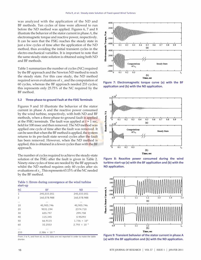
was analyzed with the application of the ND and BF methods. Ten cycles of time were allowed to run before the ND method was applied. Figures 6, 7 and 8 illustrate the behavior of the stator current in phase A, the electromagnetic torque and reactive power, respectively. It can be seen that the FSIG reaches the steady state in just a few cycles of time after the application of the ND method, thus avoiding the initial transient cycles in the electro-mechanical variables. It is important to note that the same steady-state solution is obtained using both ND and BF methods.

Table 1 summarizes the number of cycles (NC) required by the BF approach and the Newton ND method to reach the steady state. For this case study, the ND method required seven evaluations of x∞ and the computation of 60 cycles, whereas the BF approach needed 233 cycles; this represents only 25.75% of the NC required by the BF method.

5.2 Three-phase-to-ground Fault at the FSIG Terminals

Figures 9 and 10 illustrate the behavior of the stator current in phase A and the reactive power consumed by the wind turbine, respectively, with both ND and BF methods, when a three-phase-to-ground fault is applied at the FSIG terminals. The fault was applied at t = 1 sec, held for 100 msec and then removed. The ND method was applied one cycle of time after the fault was removed. It can be seen that when the BF method is applied, the system returns to its pre-fault state several cycles after the fault has been removed. However, when the ND method is applied, this is obtained in a fewer cycles than with the BF approach.

The number of cycles required to achieve the steady-state solution of the FSIG after the fault is given in Table 2. Ninety-nine cycles of time are needed by the BF approach whilst the ND method requires only 60 cycles after six evaluations of x∞. This represents 63.15% of the NC needed by the BF method.

Table 1: Errors during convergence at the wind turbine start-upNC BF ND1 245,033.051 245,033.0512 160,078.988 160,078.988... ... ...10 40,905.746 40,905.74620 9031.194 2374.71030 655.797 299.758 40 115.345 0.95293 50 66.9115 1.736 × 105 60 32.2553 2.793 × 10−9 … …233 2.386 × 10−8

From 3 to 9, and from 61 to 232 data are not reported in order to make the table shorter.

Figure 7: Electromagnetic torque curve (a) with the BF application and (b) with the ND application.

Figure 9: Transient behavior of the stator current in phase A (a) with the BF application and (b) with the ND application.

Figure 8: Reactive power consumed during the wind turbine start-up (a) with the BF application and (b) with the ND application.

Peña R, et al.: Steady-state Solution of Fixed-speed Wind Turbines

17IETE JOURNAL OF RESEARCH | VOL 57 | ISSUE 1 | JAN-FEB 2011

Table 2: Errors during convergence at the three-phase-to-ground faultNC BF ND1 251.291 251.291 10 10,789.757 20,5189.895 20 2068.487 7420.902 30 198.687 157.022 40 67.1481 0.08979 50 13.9526 1.206 × 10-7 60 3.4976 6.170 × 10-9

… …95 3.981 × 108

From 70 to 90 data are not reported in order to make the table shorter.

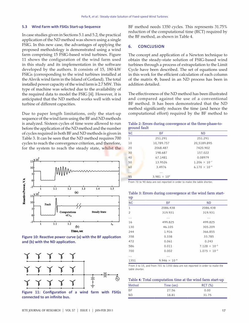
Figure 10: Reactive power curve (a) with the BF application and (b) with the ND application.

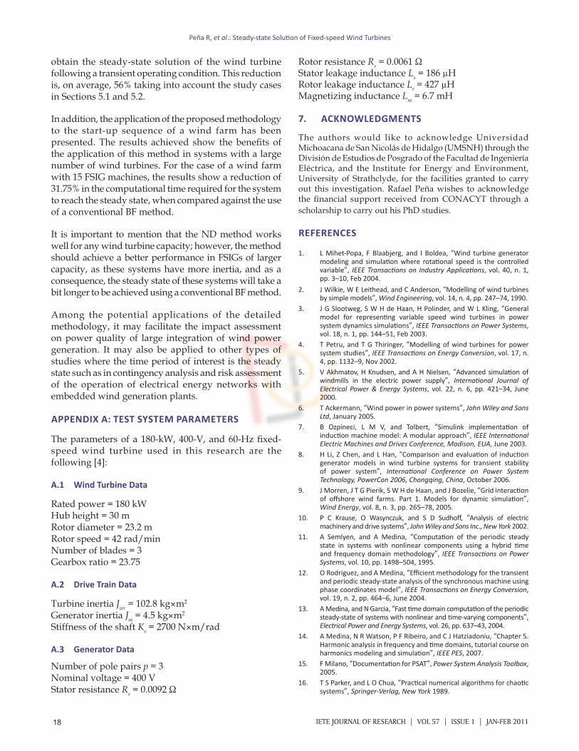
Figure 11: Configuration of a wind farm with FSIGs connected to an infinite bus.

5.3 Wind Farm with FSIGs Start-up Sequence

In case studies given in Sections 5.1 and 5.2, the practical application of the ND method was shown using a single FSIG. In this new case, the advantages of applying the proposed methodology is demonstrated using a wind farm comprising 15 FSIG-based wind turbines. Figure 11 shows the configuration of the wind farm used in this study and its implementation in the software developed by the authors. It consists of 15, 180-kW FSIGs (corresponding to the wind turbines installed at the Alsvik wind farm in the Island of Gotland). The total installed power capacity of the wind farm is 2.7 MW. This type of machine was selected due to the availability of the required data to model the FSIG [4]. However, it is anticipated that the ND method works well with wind turbine of different capacities.

Due to paper length limitations, only the start-up sequence of the wind farm using the BF and ND methods is analyzed. Sixteen cycles of time were allowed to run before the application of the ND method and the number of cycles required in both BF and ND methods is given in Table 3. It can be seen that the ND method requires 700 cycles to reach the convergence criterion, and therefore, for the system to reach the steady state, whilst the

BF method needs 1350 cycles. This represents 31.75% reduction of the computational time (RCT) required by the BF method, as shown in Table 4.

6. CONCLUSION

The concept and application of a Newton technique to obtain the steady-state solution of FSIG-based wind turbines through a process of extrapolation to the Limit Cycle have been described. The set of equations used in this work for the efficient calculation of each column of the matrix F, based in an ND process has been in addition detailed.

The effectiveness of the ND method has been illustrated and compared against the use of a conventional BF method. It has been demonstrated that the ND method significantly reduces the time (and hence the computational effort) required by the BF method to

Table 3: Errors during convergence at the wind farm start-upNC BF ND 1 2086.438 2086.438 2 319.931 319.931 … … … 16 499.825 499.825 130 46.105 305.209 244 1.916 366.855 358 0.338 33.785 472 0.061 0.243 586 0.011 7.128 × 10-5 700 0.002 1.075 × 10-9 … … 1351 9.946 × 10-8

From 3 to 15, and from 701 to 1350 data are not reported in order to make the table shorter.

Table 4: Total computation time at the wind farm start-upMethod Time (sec) RCT (%) BF 27.56 0.00 ND 18.81 31.75

Peña R, et al.: Steady-state Solution of Fixed-speed Wind Turbines

18 IETE JOURNAL OF RESEARCH | VOL 57 | ISSUE 1 | JAN-FEB 2011

obtain the steady-state solution of the wind turbine following a transient operating condition. This reduction is, on average, 56% taking into account the study cases in Sections 5.1 and 5.2.

In addition, the application of the proposed methodology to the start-up sequence of a wind farm has been presented. The results achieved show the benefits of the application of this method in systems with a large number of wind turbines. For the case of a wind farm with 15 FSIG machines, the results show a reduction of 31.75% in the computational time required for the system to reach the steady state, when compared against the use of a conventional BF method.

It is important to mention that the ND method works well for any wind turbine capacity; however, the method should achieve a better performance in FSIGs of larger capacity, as these systems have more inertia, and as a consequence, the steady state of these systems will take a bit longer to be achieved using a conventional BF method.

Among the potential applications of the detailed methodology, it may facilitate the impact assessment on power quality of large integration of wind power generation. It may also be applied to other types of studies where the time period of interest is the steady state such as in contingency analysis and risk assessment of the operation of electrical energy networks with embedded wind generation plants.

APPENDIX A: TEST SYSTEM PARAMETERS

The parameters of a 180-kW, 400-V, and 60-Hz fixed-speed wind turbine used in this research are the following [4]:

A.1 Wind Turbine Data

Rated power = 180 kW Hub height = 30 m Rotor diameter = 23.2 m Rotor speed = 42 rad/min Number of blades = 3 Gearbox ratio = 23.75

A.2 Drive Train Data

Turbine inertia Jwr = 102.8 kg×m2

Generator inertia Jm = 4.5 kg×m2

Stiffness of the shaft Ks = 2700 N×m/rad

A.3 Generator Data

Number of pole pairs p = 3 Nominal voltage = 400 V Stator resistance Rs = 0.0092 Ω

Rotor resistance Rr = 0.0061 Ω Stator leakage inductance Ls = 186 µH Rotor leakage inductance Lr = 427 µH Magnetizing inductance Lm = 6.7 mH

7. ACKNOWLEDGMENTS

The authors would like to acknowledge Universidad Michoacana de San Nicolás de Hidalgo (UMSNH) through the División de Estudios de Posgrado of the Facultad de Ingeniería Eléctrica, and the Institute for Energy and Environment, University of Strathclyde, for the facilities granted to carry out this investigation. Rafael Peña wishes to acknowledge the financial support received from CONACYT through a scholarship to carry out his PhD studies.

REFERENCES

1. L Mihet-Popa, F Blaabjerg, and I Boldea, �Wind turbine generator modeling and simulation where rotational speed is the controlled variable�, IEEE Transactions on Industry Applications, vol. 40, n. 1, pp. 3–10, Feb 2004.

2. J Wilkie, W E Leithead, and C Anderson, �Modelling of wind turbines by simple models�, Wind Engineering, vol. 14, n. 4, pp. 247–74, 1990.

3. J G Slootweg, S W H de Haan, H Polinder, and W L Kling, �General model for representing variable speed wind turbines in power system dynamics simulations�, IEEE Transactions on Power Systems, vol. 18, n. 1, pp. 144–51, Feb 2003.

4. T Petru, and T G Thiringer, �Modelling of wind turbines for power system studies�, IEEE Transactions on Energy Conversion, vol. 17, n. 4, pp. 1132–9, Nov 2002.

5. V Akhmatov, H Knudsen, and A H Nielsen, �Advanced simulation of windmills in the electric power supply�, International Journal of Electrical Power & Energy Systems, vol. 22, n. 6, pp. 421–34, June 2000.

6. T Ackermann, �Wind power in power systems�, John Wiley and Sons Ltd, January 2005.

7. B Ozpineci, L M V, and Tolbert, �Simulink implementation of induction machine model: A modular approach�, IEEE International Electric Machines and Drives Conference, Madison, EUA, June 2003.

8. H Li, Z Chen, and L Han, �Comparison and evaluation of induction generator models in wind turbine systems for transient stability of power system�, International Conference on Power System Technology, PowerCon 2006, Chongqing, China, October 2006.

9. J Morren, J T G Pierik, S W H de Haan, and J Bozelie, �Grid interaction of offshore wind farms. Part 1. Models for dynamic simulation�, Wind Energy, vol. 8, n. 3, pp. 265–78, 2005.

10. P C Krause, O Wasynczuk, and S D Sudhoff, �Analysis of electric machinery and drive systems�, John Wiley and Sons Inc., New York 2002.

11. A Semlyen, and A Medina, �Computation of the periodic steady state in systems with nonlinear components using a hybrid time and frequency domain methodology�, IEEE Transactions on Power Systems, vol. 10, pp. 1498–504, 1995.

12. O Rodriguez, and A Medina, �Efficient methodology for the transient and periodic steady-state analysis of the synchronous machine using phase coordinates model�, IEEE Transactions on Energy Conversion, vol. 19, n. 2, pp. 464–6, June 2004.

13. A Medina, and N Garcia, �Fast time domain computation of the periodic steady-state of systems with nonlinear and time-varying components�, Electrical Power and Energy Systems, vol. 26, pp. 637–43, 2004.

14. A Medina, N R Watson, P F Ribeiro, and C J Hatziadoniu, �Chapter 5. Harmonic analysis in frequency and time domains, tutorial course on harmonics modeling and simulation�, IEEE PES, 2007.

15. F Milano, �Documentation for PSAT�, Power System Analysis Toolbox, 2005.

16. T S Parker, and L O Chua, �Practical numerical algorithms for chaotic systems�, Springer-Verlag, New York 1989.

Peña R, et al.: Steady-state Solution of Fixed-speed Wind Turbines

19IETE JOURNAL OF RESEARCH | VOL 57 | ISSUE 1 | JAN-FEB 2011

AUTHORSRafael Peña was born in Morelia, Mexico in 1979. He received his B.E. and M.Sc. degrees from the Facultad de Ingeniería Eléctrica, UMSNH, Morelia, Mexico, in 2004 and 2006, respectively. Currently, he is doing his Ph.D. studies in the Division de Estudios de Posgrado of the Facultad de Ingeniería Eléctrica, UMSNH, Morelia, Mexico. His research interests include Distributed

Generation Systems based on Renewable Energy, Artificial intelligence, and Applied Computer Programming.

E-mail: rpena@faraday.fie.umich.mx

Aurelio Medina obtained his Ph.D. from the University of Canterbury, Christchurch, New Zealand in 1992. He has worked as a Post-Doctoral Fellow at the Universities of Canterbury, New Zealand (1 year) and Toronto, Canada (2 years). He joined the Facultad de Ingeniería Eléctrica, UMSNH, Morelia, Mexico in 1995 where he is at present the Head of the Division for Postgraduate

DOI: 10.4103/0377-2063.78297; Paper No. JR 451_09; Copyright © 2011 by the IETE

Studies. He is Senior Member of the IEEE. His research interests are in the Dynamic and Steady State Analysis of Power Systems.

E-mail: amedina@umich.mx

Olimpo Anaya-Lara received the B.E. and M.Sc. degrees from Instituto Tecnológico de Morelia, Morelia, México, and the Ph.D. degree from University of Glasgow, Glasgow, U.K., in 1990, 1998 and 2003, respectively. His industrial experience includes periods with Nissan Mexicana, Toluca, Mexico, and CSG Consultants, Coatzacoalcos, México. Currently, he is a Lecturer with

the Institute for Energy and Environment, University of Strathclyde, Glasgow, U.K. His research interests include Wind Generation, Power Electronics, and Stability of Mixed Generation Power Systems.

E-mail: olimpo.anaya-lara@eee.strath.ac.uk

Peña R, et al.: Steady-state Solution of Fixed-speed Wind Turbines