Embed Size (px)
Citation preview
OiV
Na
b
ARRAA
KIVPNPH
1
dnkehcecIitcpnopcmr
0h
Electric Power Systems Research 103 (2013) 92– 104
Contents lists available at SciVerse ScienceDirect
Electric Power Systems Research
jou rn al hom epage: www.elsev ier .com/ locate /epsr
n the periodic steady-state analysis of induction machinesnterfaced through VSCs using the Poincaré map method and aoltage-Behind-Reactance model
orberto Garciaa,∗, Enrique Achab
Facultad de Ingeniería Eléctrica, Universidad Michoacana de San Nicolás de Hidalgo, Ciudad Universitaria, 58030 Morelia, MexicoDepartment of Electrical Energy Engineering, Tampere University of Technology, Tekniikankatu 8 B, FI-33720 Tampere, Finland
a r t i c l e i n f o
rticle history:eceived 31 October 2012eceived in revised form 21 February 2013ccepted 10 May 2013vailable online 14 June 2013
a b s t r a c t
This paper presents the most efficient method to date to determine the periodic steady-state solutionof three-phase induction machines based on the amalgamation of the Poincaré map method and theso-called Voltage-Behind-Reactance (VBR) representation. An acceleration procedure based on the dis-cretization of the dynamic equations with the Poincaré map and the application of Newton’s methodallows locating periodic solutions. A per-unit VBR formulation, suitable for the Newton-based accelera-
eywords:nduction machineSCeriodic steady-stateewton methodsoincaré map
tion procedure, is used in this paper to ensure highly efficient solutions. To test further the robustnessand versatility of the per-unit VBR model, it is interfaced to a voltage source converter (VSC) and theresults show that the high efficiency of the new model remains unabated – this applies to both smalland large induction machines. The method is particularly useful to carry out harmonic-oriented analyseswhere the computational effort reduces dramatically compared to cases when more traditional inductionmachine models and solution approaches are employed.
armonics
. Introduction
Research work on induction machine modelling, analysis andesign continues to be areas of great interest to electrical engi-eers owing to the proliferation of new applications involving thisind of rotating machinery. The use of induction machines to gen-rate electricity using the wind as the primary energy resourceas increased very considerably over the past two decades, andontinues to receive a great deal of attention by the global powerngineering community, particularly, the newer breed of highlyontrollable induction machines based on the so-called Doubly-Fednduction Generator (DFIG) technology. More recently, an emerg-ng power transmission technology based on a variable frequencyransformer applies a wound rotor induction machine to inter-onnect power systems in an asynchronous manner. The use ofower electronics plays a key role in the integration of such tech-ology applications to ensure high performances at their intendedperational regime. However, the voltage and current harmonicsroduced by the associated power electronic converters have the
apacity to impair the performance and efficiency of the rotatingachinery, if left unchecked. Hence, it is an essential engineeringequirement to assess the harmonic impact in both the induction
∗ Corresponding author. Tel.: +52 443 3279728; fax: +52 443 3279728.E-mail addresses: [email protected] (N. Garcia), [email protected] (E. Acha).
378-7796/$ – see front matter © 2013 Elsevier B.V. All rights reserved.ttp://dx.doi.org/10.1016/j.epsr.2013.05.008
© 2013 Elsevier B.V. All rights reserved.
machine and the power grid with a view to apply corrective actionsif and when the need arises.
The study of the dynamic behavior of an induction machine maybe carried out with a state-of-the-art model based on a Voltage-Behind-Reactance representation of the induction machine whichhas shown to exhibit a superior performance than the classicalinduction machine model expressed in full phase coordinates, asreported in [1]. While the mechanical equations involved in theVBR model of the induction machine are described by the tradi-tional single rigid body system, the electric subsystem makes useof a state variable approach for an efficient, direct interface withthe external circuits [2]. This novel formulation has been used forelectromagnetic transient studies [3], extended to include the sat-uration characteristics of this machine [4]. No related informationseems to exist concerning the use of this efficient VBR inductionmachine model to the solution of harmonic-oriented problems. Inprinciple, any Electromagnetic Transients Program (EMTP) may beused to derive the periodic steady-state waveforms, which involvesintegrating the associated system of equations until a specifiedtolerance is reached. Despite the simplicity of the approach, conver-gence to the steady-state may be quite slow when solving lightlydamping components and the determination of the steady-state
becomes difficult to establish [5]. To circumvent such a problem,accelerated time domain solutions for the derivation of periodicsteady-state current and voltage waveforms have been put forward[6], with a great deal of research progress having been achieved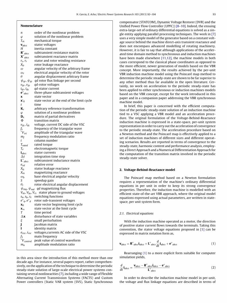
N. Garcia, E. Acha / Electric Power Syste
Nomenclature
n order of the nonlinear problemϕ solution of the nonlinear problemTm mechanical torquevabcs stator voltagesH inertia constantR′′abcs subtransient resistance matrix
X′′abcs subtransient reactance matrix
rs, rr stator and rotor winding resistanceXlr rotor leakage reactanceω angular velocity of the arbitrary frameωr electrical angular velocity of the rotor� angular displacement arbitrary frame qr, dr qd rotor flux linkage per secondvqr , vdr qd-rotor voltagesiqs, ids qd-stator currente′′abcs three-phase subtransient voltages
x state vectorx′
0 state vector at the end of the limit cyclet timeKs arbitrary reference transformationϕ solution of a nonlinear problemDx matrix of partial derivatives� transition matrixvdc , idc voltage, current DC side of the VSCfs frequency of the triangular waveˆVtri amplitude of the triangular wavemf frequency modulation ratioi column numberTrated rated torqueTe electromagnetic torqueiabcs stator currents�t integration time stepL′′abcs subtransient inductance matrix
erel relative errorXls stator leakage reactanceXm magnetizing reactanceωb base electrical angular velocityS speedup gain�r rotor electrical angular displacement mq, md qd magnetizing fluxVas, Vbs, Vcs stator phase to ground voltagessa, sb, sc switching functionse′′q, e′′d rotor sub-transient voltagesx0 state vector beginning limit cyclex∞ state vector at the limit cycleT time period�x disturbance of state variables� small perturbationJ Jacobian matrixI identity matrixevsc, ivsc voltages,currents AC side of the VSCf1 main frequencyˆV peak value of control waveform
idsstAP
iabcs = ′′ (2)
control
ma amplitude modulation ratio
n this area since the introduction of this method more than oneecade ago. For instance, several papers report, rather comprehen-ively, on the application of the technique to determine the periodic
teady-state solution of large-scale electrical power systems con-aining several nonlinearities [7], including a wide range of Flexiblelternating Current Transmission Systems (FACTS) and Customower controllers (Static VAR system (SVS), Static Synchronousms Research 103 (2013) 92– 104 93
compensator (STATCOM), Dynamic Voltage Restorer (DVR) and theUnified Power Flow Controller (UPFC)) [8–10]. Indeed, the ensuingextra-large-set of ordinary differential equations is solved as a sin-gle entity applying parallel processing techniques. The work in [7]uses a very simple model of the generator based on a constant volt-age source behind the machine direct-axis transient reactance anddoes not encompass advanced modelling of rotating machinery.However, it is fair to say that although applications of the acceler-ated time domain method to synchronous and induction machineshave been made elsewhere [11,12], the machine models in bothcases correspond to the classical phase coordinates as opposed tothe more efficient, newer generation of models based on the VBRconcept. More importantly, the results achieved by the per-unitVBR induction machine model using the Poincaré map method todetermine the periodic steady-state are shown to be far superior toany other method thus far available in the open literature. Cer-tainly, no work on acceleration to the periodic steady-state hasbeen applied to either synchronous or induction machines modelsbased on the VBR concept, except for the work introduced in thispaper and in a companion paper addressing the VBR synchronousmachine model.
In brief, this paper is concerned with the efficient computa-tion of the periodic steady-state solution of an induction machinetied to a VSC applying a VBR model and an acceleration proce-dure. The original formulation of the Voltage-Behind-Reactanceinduction machine is expressed in a state-space, per-unit systemrepresentation in order to carry out the acceleration of convergenceto the periodic steady-state. The acceleration procedure based ona Newton method and the Poincaré map is effectively applied to aset of induction machines of different sizes and different operat-ing scenarios. Results are reported in terms of convergence to thesteady-state, harmonic content and performance analysis, employ-ing a Direct Approach and a Numerical Differentiation Approach forthe computation of the transition matrix involved in the periodicsteady-state solver.
2. Voltage-Behind-Reactance model
The Poincaré map method based on a Newton formulationrequires a representation of the machine’s ordinary differentialequations in per unit in order to keep its strong convergenceproperties. Therefore, the induction machine is modelled with anefficient state-of-the-art VBR approach, where the original modelequations expressed using actual parameters, are written in state-space, per unit system form.
2.1. Electrical equations
With the induction machine operated as a motor, the directionof positive stator current flows towards the terminals. Taking thisconvention, the stator voltage equations proposed in [1] can beexpressed in matrix notation form as,
vabcs = R′′abcsiabcs + L′′
abcsd
dtiabcs + e′′
abcs (1)
Rearranging (1) to a more explicit form suitable for computersimulation yields,
d vabcs − R′′abcsiabcs − e′′
abcs
dt L abcs
In order to describe the induction machine model in per-unit,the voltage and flux linkage equations are described in terms of
9 r Syste
ru
X
R
wo
X
X
X
R
R
R
a
X
irtr
w
a
i
˙
4 N. Garcia, E. Acha / Electric Powe
eactances rather than inductances, where all quantities are in pernit. Therefore, the stator currents can be rewritten as,
d
dtiabcs = ωb
[vabcs − R′′
abcsiabcs − e′′abcs
X′′abcs
](3)
The reactance and resistance matrices are expressed as,
′′abcs =
⎡⎢⎣XS XM XM
XM XS XM
XM XM XS
⎤⎥⎦ (4)
′′abcs =
⎡⎢⎣RS RM RM
RM RS RM
RM RM RS
⎤⎥⎦ (5)
here the resistances and inductances [1] are re-written in termsf reactances as follows,
S = Xls + Xa (6)
M = −Xa2
(7)
a = 23X ′′m (8)
S = rs + Ra (9)
M = −Ra2
(10)
a = 23
(X ′′m
Xlr
)2
rr (11)
nd
′′m =
(1Xm
+ 1Xlr
)−1(12)
In the above equations, ωb is the base electrical angular veloc-ty, ωr is the electrical angular velocity of the rotor and �r is theotor electrical angular displacement. From the rotor voltage equa-ions reported in [1], the per-unit representation using an arbitraryeference frame is derived,
d
dt qr = ωb
[− rrXlr
( qr − mq
)−
(ω − ωrωb
) dr + vqr
](13)
d
dt dr = ωb
[− rrXlr
( dr − md
)−
(ω − ωrωb
) qr + vdr
](14)
here
mq = X ′′m
( qrXlr
+ iqs
)(15)
md = X ′′m
( drXlr
+ ids
)(16)
The stator currents transformed into the rotor reference framere,
qd0s = Ksiabcs (17)
ms Research 103 (2013) 92– 104
where
Ks = 23
⎡⎢⎢⎢⎢⎢⎣
cos(�)
cos(� − 2�
3
)cos
(� + 2�
3
)
sin(�)
sin(� − 2�
3
)sin
(� + 2�
3
)
12
12
12
⎤⎥⎥⎥⎥⎥⎦
(18)
The stator voltage equations are,
vabcs =[Vas Vbs Vcs
]T(19)
where Vas, Vbs and Vcs are the phase to ground voltages at thepoint of connection of the induction machine. The three-phase sub-transient voltages are,
e′′abcs = (Ks)
−1[ e′′q e′′d 0]T
(20)
with the output sub-transient voltages of the rotor model definedas,
e′′q = ωrωb
X ′′m
Xlr dr + rrX ′′
m
(Xlr)2
(X ′′m
Xlr− 1
) qr + X ′′
m
Xlrvqr (21)
e′′d = −ωrωb
X ′′m
Xlr qr + rrX ′′
m
(Xlr)2
(X ′′m
Xlr− 1
) dr + X ′′
m
Xlrvdr (22)
2.2. Mechanical equations
The rotor speed is computed as follows,
d
dt
(ωrωb
)= Te − Tm
2H(23)
where Tm is the mechanical torque and the per unit electromagnetictorque is defined as [13],
Te = mdiqs − mqids (24)
The rotor position is defined as,
d
dt�r = ωb
(ωrωb
)(25)
2.3. State-space model
The state variable representation of the induction machine canbe described using a state-space representation as follows,
x = Ax + N (x) + Bu (26)
The linear terms involved in the induction machine model are
contained in matrix A, while the nonlinear terms are separatedand placed in the arrangement N (x). Besides, matrix B containsthe inputs to the induction machine. Hence, Eq. (26) can also beexpanded as shown in (26b).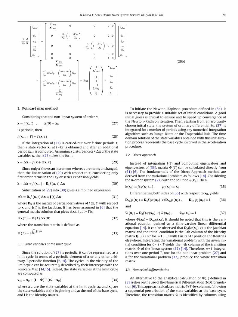
r Syste
iabcs
qr
dr
ωrωb
�r
3
˙x
i
f
tpv
˙x
tfi
˙x
�
wtg
�
w
�
3
ltlPa
x
wta
˙
˙
N. Garcia, E. Acha / Electric Powe
1ωb
d
dt
⎡⎢⎢⎢⎢⎢⎢⎢⎣
iabcs
qr
dr
ωrωb
�r
⎤⎥⎥⎥⎥⎥⎥⎥⎦
=
⎡⎢⎢⎢⎢⎢⎢⎢⎢⎢⎣
− R′′abcs
X′′abcs
0 0 0 0
0 − rrXlr
(1 − X ′′
m
Xlr
)0 0 0
0 0 − rrXlr
(1 − X ′′
m
Xlr
)0 0
0 0 0 0 0
0 0 0 1 0
⎤⎥⎥⎥⎥⎥⎥⎥⎥⎥⎦
⎡⎢⎢⎢⎢⎢⎢⎢⎣
−
⎡⎢⎢⎢⎢⎢⎢⎢⎢⎢⎢⎢⎣
e′′abcs
X′′abcs
−rrXlrX ′′miqs +
(ω − ωrωb
) dr
−rrXlrX ′′mids +
(ω − ωrωb
) qr
−Te2Hωb
0
⎤⎥⎥⎥⎥⎥⎥⎥⎥⎥⎥⎥⎦
+ diag
⎛⎜⎜⎜⎜⎜⎜⎝
1X′′
abcs
1
1−1
2Hωb
0
⎞⎟⎟⎟⎟⎟⎟⎠
·
⎡⎢⎢⎢⎢⎢⎢⎣
vabcs
vqr
vdr
Tm
0
⎤⎥⎥⎥⎥⎥⎥⎦
. Poincaré map method
Considering that the non-linear system of order n,
= f (x, t) , x (0) = x0 (27)
s periodic, then
(x, t + T) = f (x, t) (28)
If the integration of (27) is carried-out over k time periods T,hen a state vector xk at t = kT is obtained and after an additionaleriod xk+1 is computed. Assuming a disturbance x + �x of the stateariables x, then (27) takes the form,
+ �˙x = f (x + �x, t) (29)
Since only x shows an increment whereas t remains unchanged,hen the linearization of (29) with respect to x, considering onlyrst order terms in the Taylor series expansion yields,
+ �˙x ≈ f (x, t) + Dxf (x, t)�x (30)
Substitution of (27) into (30) gives a simplified expression
˙x ≈ Dxf (x, t)�x = J (t)�x (31)
here Dx is the matrix of partial derivatives of f (x, t) with respecto x and J (t) is the Jacobian. It has been assumed in [6] that theeneral matrix solution that gives �x (t) at t = T is,
x (T) = � (T)�x (0) (32)
here the transition matrix is defined as
(T) = e
∫ T
0J(t)dt
(33)
.1. State variables at the limit cycle
Since the solution of (27) is periodic, it can be represented as aimit cycle in terms of a periodic element of x or any other arbi-rary T-periodic function [6,14]. The cycles in the vicinity of theimit cycle can be accurately described by their intercepts with theoincaré Map [14,15]. Indeed, the state variables at the limit cyclere computed as,
∞ = x0 + (I − �)−1(x′0 − x0) (34)
here x∞ are the state variables at the limit cycle, x0 and x′0 are
he state variables at the beginning and at the end of the base cycle,nd I is the identity matrix.
ms Research 103 (2013) 92– 104 95
⎤⎥⎥⎥⎥⎥⎥⎥⎦
(26b)
To initiate the Newton–Raphson procedure defined in (34), itis necessary to provide a suitable set of initial conditions. A goodinitial guess is crucial to ensure and to speed up convergence ofthe Newton–Raphson iteration. Then, starting from an arbitrarilychosen initial state, the system of ordinary differential Eq. (27) isintegrated for a number of periods using any numerical integrationalgorithm such as Runge–Kutta or the Trapezoidal Rule. The timedomain solution of the state variables obtained with this initializa-tion process represents the base cycle involved in the accelerationprocedure.
3.2. Direct approach
Instead of integrating J (t) and computing eigenvalues andeigenvectors of (33), matrix � (T) can be calculated directly from(31) [6]. The fundamentals of the Direct Approach method arederived from the variational problem as follows [14]. Consideringthe n-order system (27) with the solution ϕ(x0). Then,
ϕ(x0) = f (ϕ(x0), t) , ϕ0(x0) = x0 (35)
Differentiating both sides of (35) with respect to x0, yields,
Dx0 ˙ϕ (x0) = Dxf (ϕ (x0) , t) Dx0ϕ (x0) , Dx0ϕ0 (x0) = I (36)
and
� (x0) = Dxf (ϕ (x0) , t)� (x0) , �0 (x0) = I (37)
where �(x0) = Dx0ϕ(x0). It should be noted that this is the vari-ational equation defined as a time-varying linear differentialequation [14]. It can be observed that Dxf(ϕ(x0), t) is the Jacobianmatrix and the initial condition is the i-th column of the identitymatrix I(:, i) ∈ R
n for i = 1 . . . n with 1 in its i-th position and 0 entrieselsewhere. Integrating the variational problem with the given ini-tial condition for 0 ≤ t ≤ T yields the i-th column of the transitionmatrix � of the linear system (37) [14]. Therefore, n + 1 integra-tions over one period T, one for the nonlinear problem (27) andn for the variational problem (37), produce the whole transitionmatrix.
3.3. Numerical differentiation
An alternative to the analytical calculation of �(T) defined in
(33) relies on the use of the Numerical Differentiation (ND) formula-tion [6]. This approach calculates matrix �(T) by columns, followinga sequential perturbation of the state variables at the base cycle.Therefore, the transition matrix � is identified by columns using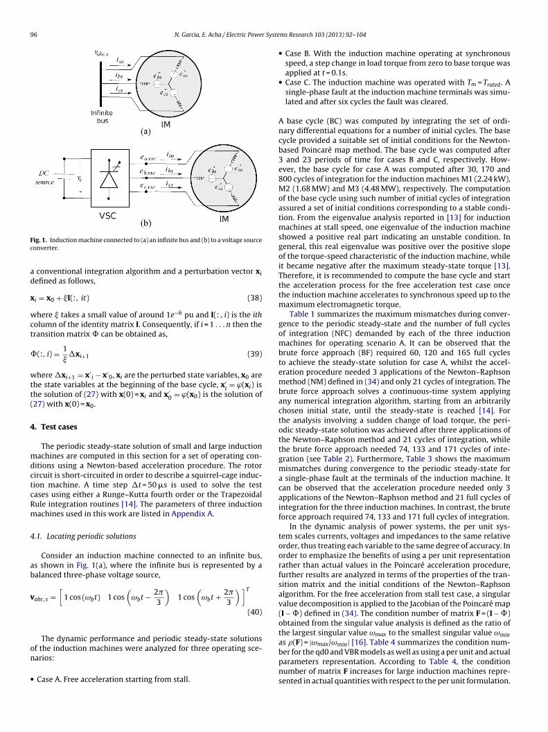
96 N. Garcia, E. Acha / Electric Power Syste
Fc
ad
x
wct
�
wtt(
4
mdctcRm
4
ab
v
on
•
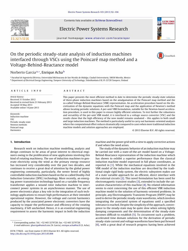
ig. 1. Induction machine connected to (a) an infinite bus and (b) to a voltage sourceonverter.
conventional integration algorithm and a perturbation vector xiefined as follows,
i = x0 + �I(:, it) (38)
here � takes a small value of around 1e−6 pu and I(: , i) is the itholumn of the identity matrix I. Consequently, if i = 1 . . . n then theransition matrix � can be obtained as,
(:, i) = 1��xi+1 (39)
here �xi+1 = x′i − x′
0, xi are the perturbed state variables, x0 arehe state variables at the beginning of the base cycle, x′
i= ϕ(xi) is
he solution of (27) with x(0) = xi and x′0 = ϕ(x0) is the solution of
27) with x(0) = x0.
. Test cases
The periodic steady-state solution of small and large inductionachines are computed in this section for a set of operating con-
itions using a Newton-based acceleration procedure. The rotorircuit is short-circuited in order to describe a squirrel-cage induc-ion machine. A time step �t = 50 �s is used to solve the testases using either a Runge–Kutta fourth order or the Trapezoidalule integration routines [14]. The parameters of three inductionachines used in this work are listed in Appendix A.
.1. Locating periodic solutions
Consider an induction machine connected to an infinite bus,s shown in Fig. 1(a), where the infinite bus is represented by aalanced three-phase voltage source,
abc,s =[
1 cos (ωbt) 1 cos(ωbt − 2�
3
)1 cos
(ωbt + 2�
3
)]T(40)
The dynamic performance and periodic steady-state solutionsf the induction machines were analyzed for three operating sce-
arios:Case A. Free acceleration starting from stall.
ms Research 103 (2013) 92– 104
• Case B. With the induction machine operating at synchronousspeed, a step change in load torque from zero to base torque wasapplied at t = 0.1s.
• Case C. The induction machine was operated with Tm = Trated. Asingle-phase fault at the induction machine terminals was simu-lated and after six cycles the fault was cleared.
A base cycle (BC) was computed by integrating the set of ordi-nary differential equations for a number of initial cycles. The basecycle provided a suitable set of initial conditions for the Newton-based Poincaré map method. The base cycle was computed after3 and 23 periods of time for cases B and C, respectively. How-ever, the base cycle for case A was computed after 30, 170 and800 cycles of integration for the induction machines M1 (2.24 kW),M2 (1.68 MW) and M3 (4.48 MW), respectively. The computationof the base cycle using such number of initial cycles of integrationassured a set of initial conditions corresponding to a stable condi-tion. From the eigenvalue analysis reported in [13] for inductionmachines at stall speed, one eigenvalue of the induction machineshowed a positive real part indicating an unstable condition. Ingeneral, this real eigenvalue was positive over the positive slopeof the torque-speed characteristic of the induction machine, whileit became negative after the maximum steady-state torque [13].Therefore, it is recommended to compute the base cycle and startthe acceleration process for the free acceleration test case oncethe induction machine accelerates to synchronous speed up to themaximum electromagnetic torque.
Table 1 summarizes the maximum mismatches during conver-gence to the periodic steady-state and the number of full cyclesof integration (NFC) demanded by each of the three inductionmachines for operating scenario A. It can be observed that thebrute force approach (BF) required 60, 120 and 165 full cyclesto achieve the steady-state solution for case A, whilst the accel-eration procedure needed 3 applications of the Newton–Raphsonmethod (NM) defined in (34) and only 21 cycles of integration. Thebrute force approach solves a continuous-time system applyingany numerical integration algorithm, starting from an arbitrarilychosen initial state, until the steady-state is reached [14]. Forthe analysis involving a sudden change of load torque, the peri-odic steady-state solution was achieved after three applications ofthe Newton–Raphson method and 21 cycles of integration, whilethe brute force approach needed 74, 133 and 171 cycles of inte-gration (see Table 2). Furthermore, Table 3 shows the maximummismatches during convergence to the periodic steady-state fora single-phase fault at the terminals of the induction machine. Itcan be observed that the acceleration procedure needed only 3applications of the Newton–Raphson method and 21 full cycles ofintegration for the three induction machines. In contrast, the bruteforce approach required 74, 133 and 171 full cycles of integration.
In the dynamic analysis of power systems, the per unit sys-tem scales currents, voltages and impedances to the same relativeorder, thus treating each variable to the same degree of accuracy. Inorder to emphasize the benefits of using a per unit representationrather than actual values in the Poincaré acceleration procedure,further results are analyzed in terms of the properties of the tran-sition matrix and the initial conditions of the Newton–Raphsonalgorithm. For the free acceleration from stall test case, a singularvalue decomposition is applied to the Jacobian of the Poincaré map(I − �) defined in (34). The condition number of matrix F = (I − �)obtained from the singular value analysis is defined as the ratio ofthe largest singular value ωmax to the smallest singular value ωminas (F) = |ωmax/ωmin| [16]. Table 4 summarizes the condition num-
ber for the qd0 and VBR models as well as using a per unit and actualparameters representation. According to Table 4, the conditionnumber of matrix F increases for large induction machines repre-sented in actual quantities with respect to the per unit formulation.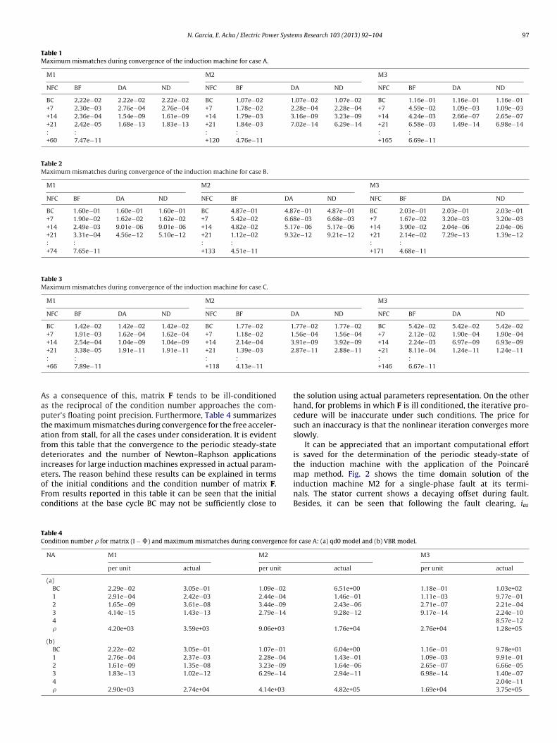
N. Garcia, E. Acha / Electric Power Systems Research 103 (2013) 92– 104 97
Table 1Maximum mismatches during convergence of the induction machine for case A.
M1 M2 M3
NFC BF DA ND NFC BF DA ND NFC BF DA ND
BC 2.22e−02 2.22e−02 2.22e−02 BC 1.07e−02 1.07e−02 1.07e−02 BC 1.16e−01 1.16e−01 1.16e−01+7 2.30e−03 2.76e−04 2.76e−04 +7 1.78e−02 2.28e−04 2.28e−04 +7 4.59e−02 1.09e−03 1.09e−03+14 2.36e−04 1.54e−09 1.61e−09 +14 1.79e−03 3.16e−09 3.23e−09 +14 4.24e−03 2.66e−07 2.65e−07+21 2.42e−05 1.68e−13 1.83e−13 +21 1.84e−03 7.02e−14 6.29e−14 +21 6.58e−03 1.49e−14 6.98e−14: : : : : :+60 7.47e−11 +120 4.76e−11 +165 6.69e−11
Table 2Maximum mismatches during convergence of the induction machine for case B.
M1 M2 M3
NFC BF DA ND NFC BF DA ND NFC BF DA ND
BC 1.60e−01 1.60e−01 1.60e−01 BC 4.87e−01 4.87e−01 4.87e−01 BC 2.03e−01 2.03e−01 2.03e−01+7 1.90e−02 1.62e−02 1.62e−02 +7 5.42e−02 6.68e−03 6.68e−03 +7 1.67e−02 3.20e−03 3.20e−03+14 2.49e−03 9.01e−06 9.01e−06 +14 4.82e−02 5.17e−06 5.17e−06 +14 3.90e−02 2.04e−06 2.04e−06+21 3.31e−04 4.56e−12 5.10e−12 +21 1.12e−02 9.32e−12 9.21e−12 +21 2.14e−02 7.29e−13 1.39e−12: : : : : :+74 7.65e−11 +133 4.51e−11 +171 4.68e−11
Table 3Maximum mismatches during convergence of the induction machine for case C.
M1 M2 M3
NFC BF DA ND NFC BF DA ND NFC BF DA ND
BC 1.42e−02 1.42e−02 1.42e−02 BC 1.77e−02 1.77e−02 1.77e−02 BC 5.42e−02 5.42e−02 5.42e−02+7 1.91e−03 1.62e−04 1.62e−04 +7 1.18e−02 1.56e−04 1.56e−04 +7 2.12e−02 1.90e−04 1.90e−04+14 2.54e−04 1.04e−09 1.04e−09 +14 2.14e−04 3.91e−09 3.92e−09 +14 2.24e−03 6.97e−09 6.93e−09+21 3.38e−05 1.91e−11 1.91e−11 +21 1.39e−03 2.87e−11 2.88e−11 +21 8.11e−04 1.24e−11 1.24e−11
AaptafdieoFc
TC
: : : :
+66 7.89e−11 +118 4.13e−11
s a consequence of this, matrix F tends to be ill-conditioneds the reciprocal of the condition number approaches the com-uter’s floating point precision. Furthermore, Table 4 summarizeshe maximum mismatches during convergence for the free acceler-tion from stall, for all the cases under consideration. It is evidentrom this table that the convergence to the periodic steady-stateeteriorates and the number of Newton–Raphson applications
ncreases for large induction machines expressed in actual param-ters. The reason behind these results can be explained in terms
f the initial conditions and the condition number of matrix F.rom results reported in this table it can be seen that the initialonditions at the base cycle BC may not be sufficiently close toable 4ondition number for matrix (I − �) and maximum mismatches during convergence fo
NA M1 M2
per unit actual per unit
(a)BC 2.29e−02 3.05e−01 1.09e−02
1 2.91e−04 2.42e−03 2.44e−04
2 1.65e−09 3.61e−08 3.44e−09
3 4.14e−15 1.43e−13 2.79e−14
4
4.20e+03 3.59e+03 9.06e+03
(b)BC 2.22e−02 3.05e−01 1.07e−01
1 2.76e−04 2.37e−03 2.28e−04
2 1.61e−09 1.35e−08 3.23e−09
3 1.83e−13 1.02e−12 6.29e−14
4
2.90e+03 2.74e+04 4.14e+03
: :+146 6.67e−11
the solution using actual parameters representation. On the otherhand, for problems in which F is ill conditioned, the iterative pro-cedure will be inaccurate under such conditions. The price forsuch an inaccuracy is that the nonlinear iteration converges moreslowly.
It can be appreciated that an important computational effortis saved for the determination of the periodic steady-state ofthe induction machine with the application of the Poincarémap method. Fig. 2 shows the time domain solution of the
induction machine M2 for a single-phase fault at its termi-nals. The stator current shows a decaying offset during fault.Besides, it can be seen that following the fault clearing, iasr case A: (a) qd0 model and (b) VBR model.
M3
actual per unit actual
6.51e+00 1.18e−01 1.03e+021.46e−01 1.11e−03 9.77e−012.43e−06 2.71e−07 2.21e−049.28e−12 9.17e−14 2.24e−10
8.57e−121.76e+04 2.76e+04 1.28e+05
6.04e+00 1.16e−01 9.78e+011.43e−01 1.09e−03 9.91e−011.64e−06 2.65e−07 6.66e−052.94e−11 6.98e−14 1.40e−07
2.04e−114.82e+05 1.69e+04 3.75e+05
98 N. Garcia, E. Acha / Electric Power Systems Research 103 (2013) 92– 104
Fig. 2. Stator current for the induction machine M2 for a single-phase fault at phase A: (a) transient solution and (b) steady-state solution.
Table 5Maximum mismatches during convergence of induction machines under unbalanced voltage: (a) sag type-B and (b) sag type-C.
M1 M2 M3
NFC BF DA ND NFC BF DA ND NFC BF DA ND
(a)BC 7.47e−03 7.47e−03 7.47e−03 BC 3.74e−02 3.74e−02 3.74e−02 BC 2.75e−02 2.75e−02 2.75e−02+7 1.60e−03 1.11e−04 1.11e−04 +7 4.69e−03 1.03e−04 1.03e−04 +7 5.28e−03 8.76e−05 8.76e−05+14 2.45e−04 4.15e−10 4.31e−10 +14 1.23e−03 5.21e−10 5.36e−10 +14 1.16e−03 3.97e−09 3.99e−09+21 3.76e−05 2.15e−14 2.55e−14 +21 3.37e−04 3.11e−14 1.15e−14 +21 3.94e−04 9.99e−15 1.65e−14: : : : : :+69 9.81e−11 +113 6.18e−11 +137 5.05e−11
(b)BC 3.39e−02 3.39e−02 3.39e−02 BC 2.91e−02 2.91e−02 2.91e−02 BC 2.38e−02 2.38e−02 2.38e−02+7 1.56e−03 1.15e−04 1.15e−04 +7 5.56e−03 2.91e−04 2.91e−04 +7 3.71e−03 3.20e−05 3.20e−05+14 2.39e−04 1.28e−09 1.32e−09 +14 4.57e−04 8.82e−09 8.88e−09 +14 8.03e−04 1.40e−08 1.41e−08
1.04e−14 2.17e−14 +21 1.51e−04 2.28e−14 1.14e−14: :+125 9.52e−11
utaot
4
taTac
vvtai6(tfcasmP
Table 6Percent of total harmonic distortion at selected variables of the induction machineunder unbalanced voltage.
sag type-B sag type-C
M1 M2 M3 M1 M2 M3
ia 0.5144 0.4784 0.4800 0.5044 0.4944 0.4946
+21 3.67e−05 3.26e−14 1.75e−14 +21 6.37e−04
: : : :
+69 9.59e−11 +117 2.05e−11
ndergoes sustained oscillations. It can be observed from Fig. 2hat the proposal presented in this work predicted transientnd periodic steady-state responses that are identical to thosef the power-systems-computer-aided-design/electromagnetic-ransients-program-for-DC simulation (PSCAD/EMTDC) [17].
.2. Operation under unbalanced voltage
In this section, a test case is carried out in order to determineorque pulsations and harmonic content that may arise from oper-ting the induction machine under unbalanced supply conditions.he induction machine is operated with a rated load torque andn unbalanced voltage, which consists of type-B and type-C sagonditions [18] with 3% voltage unbalance.
Table 5 summarizes the maximum mismatches during con-ergence of the induction machine operated under unbalancedoltage. Results reported in Table 5 correspond to three induc-ion machines reported in Appendix A. While the DA and NDpproaches required three applications of the Newton–Raphsonteration for type-B voltage sag, the brute force approach needed9, 113 and 137 NFC for induction machines M1, M2 and M3see Table 5(a)). In addition, it can be seen from Table 5(b)hat the brute force approach required 69, 117 and 125 NFCor type-C voltage sag. On the contrary, the acceleration pro-edure based on the DA and ND approaches needed only 3
pplications of the Newton iteration. Fig. 3 depicts the periodicteady-state waveforms of the stator currents and the electro-agnetic torque obtained with the Poincaré map method andSCAD/EMTDC. It can be noted that the periodic steady-state
ω 0.0225 0.0131 0.0030 0.0225 0.0131 0.0030Te 22.8843 13.1816 12.2280 22.8683 13.1849 12.2319
waveforms obtained with the acceleration procedure matchedresults obtained with PSCAD/EMTDC very closely. It can beappreciated that the pulsating torque was dominated by thesecond harmonic component of the alternating current (AC) sourcefrequency [19]. The amplitude of the pulsating toque is 8.225 kNm.These results show that the stator supply asymmetry produced adouble supply frequency harmonic in the torque spectrum. Themagnitude of the pulsating torque is not negligible and, there-fore, minimization of this component will benefit the operationand integrity of the induction machine.
The periodic steady-state waveforms reported in Fig. 3, rep-resented by sets of discrete values at equally spaced intervals,were subjected to Fast Fourier Transformation (FFT) processingto derive the harmonic spectra. Table 6 summarizes the percentof total harmonic distortion (%THD) for stator current at phase
A, rotor speed and electromagnetic torque. These results indicatethat the presence of unbalance in the stator circuit caused a risein the harmonic distortion when compared to induction machineoperation with balanced excitation. The effect of an unbalanced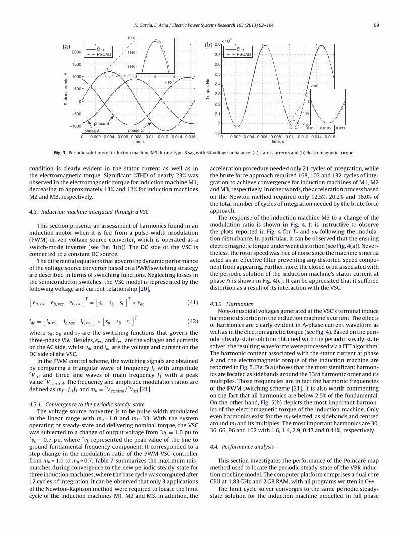
N. Garcia, E. Acha / Electric Power Systems Research 103 (2013) 92– 104 99
ith 3%
ctodM
4
i(sc
oatf[
i
wtoD
bˆvd
4
iowˆgsfmt1oc
Fig. 3. Periodic solutions of induction machine M3 during type-B sag w
ondition is clearly evident in the stator current as well as inhe electromagnetic torque. Significant %THD of nearly 23% wasbserved in the electromagnetic torque for induction machine M1,ecreasing to approximately 13% and 12% for induction machines2 and M3, respectively.
.3. Induction machine interfaced through a VSC
This section presents an assessment of harmonics found in annduction motor when it is fed from a pulse-width modulationPWM)-driven voltage source converter, which is operated as awitch-mode inverter (see Fig. 1(b)). The DC side of the VSC isonnected to a constant DC source.
The differential equations that govern the dynamic performancef the voltage source converter based on a PWM switching strategyre described in terms of switching functions. Neglecting losses inhe semiconductor switches, the VSC model is represented by theollowing voltage and current relationship [20],
ea,vsc eb,vsc ec,vsc]T =
[sa sb sc
]T × vdc (41)
dc =[ia,vsc ib,vsc ic,vsc
]×
[sa sb sc
]T(42)
here sa, sb and sc are the switching functions that govern thehree-phase VSC. Besides, evsc and ivsc are the voltages and currentsn the AC side, whilst vdc and idc are the voltage and current on theC side of the VSC.
In the PWM control scheme, the switching signals are obtainedy comparing a triangular wave of frequency fs with amplitudeVtri and three sine waves of main frequency f1 with a peakalue ˆVcontrol . The frequency and amplitude modulation ratios areefined as mf = fs/f1 and ma = ˆVcontrol/ˆVtri [21].
.3.1. Convergence to the periodic steady-stateThe voltage source converter is to be pulse-width modulated
n the linear range with ma = 1.0 and mf = 33. With the systemperating at steady-state and delivering nominal torque, the VSCas subjected to a change of output voltage from ˆvL = 1.0 pu to
vL = 0.7 pu, where ˆvL represented the peak value of the line toround fundamental frequency component. It corresponded to atep change in the modulation ratio of the PWM-VSC controllerrom ma = 1.0 to ma = 0.7. Table 7 summarizes the maximum mis-
atches during convergence to the new periodic steady-state for
hree induction machines, where the base cycle was computed after2 cycles of integration. It can be observed that only 3 applicationsf the Newton–Raphson method were required to locate the limitycle of the induction machines M1, M2 and M3. In addition, thevoltage unbalance: (a) stator currents and (b)electromagnetic torque.
acceleration procedure needed only 21 cycles of integration, whilethe brute force approach required 168, 103 and 132 cycles of inte-gration to achieve convergence for induction machines of M1, M2and M3, respectively. In other words, the acceleration process basedon the Newton method required only 12.5%, 20.2% and 16.0% ofthe total number of cycles of integration needed by the brute forceapproach.
The response of the induction machine M3 to a change of themodulation ratio is shown in Fig. 4. It is instructive to observethe plots reported in Fig. 4 for Te and ωr following the modula-tion disturbance. In particular, it can be observed that the ensuingelectromagnetic torque underwent distortion (see Fig. 4(a)). Never-theless, the rotor speed was free of noise since the machine’s inertiaacted as an effective filter preventing any distorted speed compo-nent from appearing. Furthermore, the closed orbit associated withthe periodic solution of the induction machine’s stator current atphase A is shown in Fig. 4(c). It can be appreciated that it suffereddistortion as a result of its interaction with the VSC.
4.3.2. HarmonicsNon-sinusoidal voltages generated at the VSC’s terminal induce
harmonic distortion in the induction machine’s current. The effectsof harmonics are clearly evident in A-phase current waveform aswell as in the electromagnetic torque (see Fig. 4). Based on the peri-odic steady-state solution obtained with the periodic steady-statesolver, the resulting waveforms were processed via a FFT algorithm.The harmonic content associated with the stator current at phaseA and the electromagnetic torque of the induction machine arereported in Fig. 5. Fig. 5(a) shows that the most significant harmon-ics are located as sidebands around the 33rd harmonic order and itsmultiples. Those frequencies are in fact the harmonic frequenciesof the PWM switching scheme [21]. It is also worth commentingon the fact that all harmonics are below 2.5% of the fundamental.On the other hand, Fig. 5(b) depicts the most important harmon-ics of the electromagnetic torque of the induction machine. Onlyeven harmonics exist for the mf selected, as sidebands and centredaround mf and its multiples. The most important harmonics are 30,36, 66, 96 and 102 with 1.6, 1.4, 2.9, 0.47 and 0.44%, respectively.
4.4. Performance analysis
This section investigates the performance of the Poincaré mapmethod used to locate the periodic steady-state of the VBR induc-
tion machine model. The computer platform comprises a dual coreCPU at 1.83 GHz and 2 GB RAM, with all programs written in C++.The limit cycle solver converges to the same periodic steady-state solution for the induction machine modelled in full phase

100 N. Garcia, E. Acha / Electric Power Systems Research 103 (2013) 92– 104
Table 7Maximum mismatches during convergence of the induction machine and a VSC for a change of the output voltage.
M1 M2 M3
NFC BF DA ND NFC BF DA ND NFC BF DA ND
BC 2.14e−02 2.14e−02 2.14e−02 BC 2.44e−02 2.44e−02 2.44e−02 BC 1.72e−02 1.72e−02 1.72e−02+7 9.24e−03 3.73e−03 3.73e−03 +7 6.31e−03 5.37e−04 5.37e−04 +7 9.22e−03 2.02e−03 2.02e−03+14 4.07e−03 1.29e−06 1.29e−06 +14 1.44e−03 4.61e−07 4.61e−07 +14 4.73e−03 7.08e−06 7.09e−06+21 1.81e−03 5.48e−12 5.68e−12 +21 3.62e−04 9.90e−12 1.02e−11 +21 1.81e−03 5.25e−11 4.23e−11: : : : : :+168 9.19e−11 +103 6.04e−11 +132 9.29e−11
0.15 0.2 0.25 0.3 0.35 0.4 0.45−4
−2
0
2
4
6x 10
4
time, s
Te,
Nm
Base cycle
Change of output voltage
Steady−state
Steady−state
0.15 0.2 0.25 0.3 0.35 0.4 0.451774
1776
1778
1780
1782
1784
1786
1788
1790
time, s
wr,
r/m
in
−6 −4 −2 0 2 4 6−1.5
−1
−0.5
0
0.5
1
1.5
Source, KV
Cur
rent
pha
se A
, KA
(a) (b)
(c)
Fig. 4. Selected variables of the induction machine M3 during a change of PWM modulation ratio: (a) time domain solution for electromagnetic torque, (b) time domainsolution for rotor speed and (c) periodic solution for stator current at phase A.
0 33 66 990
0.5
1
1.5
2
2.5
Harmonic
Mag
nitu
de, %
of F
und.
0 33 66 990
0.5
1
1.5
2
2.5
3
Harmonic
Mag
nitu
de, %
of D
C c
ompo
nent
(a) (b)
Fig. 5. Harmonic content for induction machine M3 (a) stator current at phase A and (b) electromagnetic torque.
N. Garcia, E. Acha / Electric Power Syste
10−6
10−5
10−4
10−10
10−8
10−6
10−4
Rel
ativ
e er
ror,
%
NM−PD, Runge−KuttaNM−VBR, Runge−KuttaNM−PD, Trapezoidal RuleNM−VBR, Trapezoidal Rule
FD
dioPwtVic1eaoofairimaTwtmaN
the DA method and a stationary frame of reference (DA-STAT) pro-
Time step, s
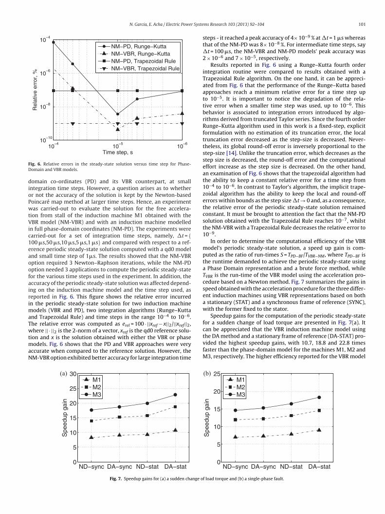
ig. 6. Relative errors in the steady-state solution versus time step for Phase-omain and VBR models.
omain co-ordinates (PD) and its VBR counterpart, at smallntegration time steps. However, a question arises as to whetherr not the accuracy of the solution is kept by the Newton-basedoincaré map method at larger time steps. Hence, an experimentas carried-out to evaluate the solution for the free accelera-
ion from stall of the induction machine M1 obtained with theBR model (NM-VBR) and with an induction machine modelled
n full phase-domain coordinates (NM-PD). The experiments werearried-out for a set of integration time steps, namely, �t = {00 �s,50 �s,10 �s,5 �s,1 �s} and compared with respect to a ref-rence periodic steady-state solution computed with a qd0 modelnd small time step of 1�s. The results showed that the NM-VBRption required 3 Newton–Raphson iterations, while the NM-PDption needed 3 applications to compute the periodic steady-stateor the various time steps used in the experiment. In addition, theccuracy of the periodic steady-state solution was affected depend-ng on the induction machine model and the time step used, aseported in Fig. 6. This figure shows the relative error incurredn the periodic steady-state solution for two induction machine
odels (VBR and PD), two integration algorithms (Runge–Kuttand Trapezoidal Rule) and time steps in the range 10−4 to 10−6.he relative error was computed as erel = 100 · ||xref − x||2/||xref||2,here || · ||2 is the 2-norm of a vector, xref is the qd0 reference solu-
ion and x is the solution obtained with either the VBR or phase
odels. Fig. 6 shows that the PD and VBR approaches were veryccurate when compared to the reference solution. However, theM-VBR option exhibited better accuracy for large integration time
ND−sync DA−sync ND−stat DA−stat0
5
10
15
20
25
30
Spe
edup
gai
n
M1M2M3
(a)
Fig. 7. Speedup gains for (a) a sudden change o
ms Research 103 (2013) 92– 104 101
steps - it reached a peak accuracy of 4× 10⁻⁹ % at �t = 1 �s whereasthat of the NM-PD was 8× 10⁻⁸ %. For intermediate time steps, say�t = 100 �s, the NM-VBR and NM-PD models’ peak accuracy was2 × 10−6 and 7 × 10⁻⁵, respectively.
Results reported in Fig. 6 using a Runge–Kutta fourth orderintegration routine were compared to results obtained with aTrapezoidal Rule algorithm. On the one hand, it can be appreci-ated from Fig. 6 that the performance of the Runge–Kutta basedapproaches reach a minimum relative error for a time step upto 10−5. It is important to notice the degradation of the rela-tive error when a smaller time step was used, up to 10−6. Thisbehavior is associated to integration errors introduced by algo-rithms derived from truncated Taylor series. Since the fourth orderRunge–Kutta algorithm used in this work is a fixed-step, explicitformulation with no estimation of its truncation error, the localtruncation error decreased as the step-size is decreased. Never-theless, its global round-off error is inversely proportional to thestep-size [14]. Unlike the truncation error, which decreases as thestep size is decreased, the round-off error and the computationaleffort increase as the step size is decreased. On the other hand,an examination of Fig. 6 shows that the trapezoidal algorithm hadthe ability to keep a constant relative error for a time step from10−4 to 10−6. In contrast to Taylor’s algorithm, the implicit trape-zoidal algorithm has the ability to keep the local and round-offerrors within bounds as the step size �t → 0 and, as a consequence,the relative error of the periodic steady-state solution remainedconstant. It must be brought to attention the fact that the NM-PDsolution obtained with the Trapezoidal Rule reaches 10−7, whilstthe NM-VBR with a Trapezoidal Rule decreases the relative error to10−9.
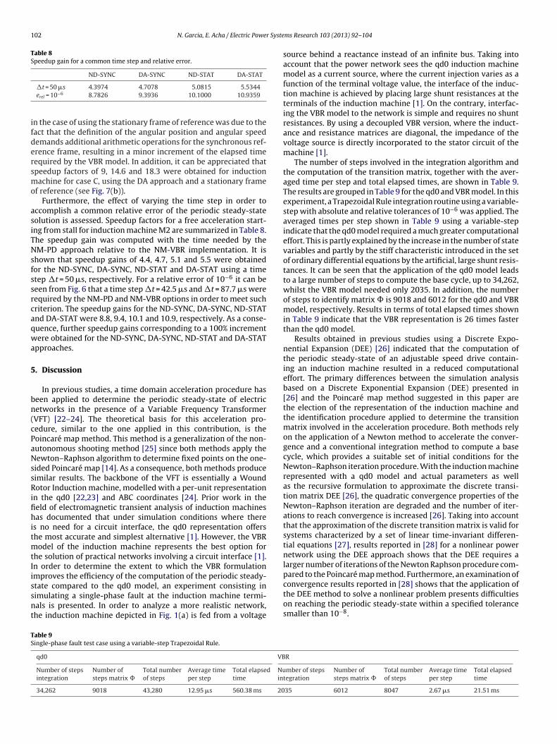
In order to determine the computational efficiency of the VBRmodel’s periodic steady-state solution, a speed up gain is com-puted as the ratio of run-times S = TPD−BF/TVBR−NM, where TPD−BF isthe runtime demanded to achieve the periodic steady-state usinga Phase Domain representation and a brute force method, whileTVBR is the run-time of the VBR model using the acceleration pro-cedure based on a Newton method. Fig. 7 summarizes the gains inspeed obtained with the acceleration procedure for the three differ-ent induction machines using VBR representations based on botha stationary (STAT) and a synchronous frame of reference (SYNC),with the former fixed to the stator.
Speedup gains for the computation of the periodic steady-statefor a sudden change of load torque are presented in Fig. 7(a). Itcan be appreciated that the VBR induction machine model using
vided the highest speedup gains, with 10.7, 18.8 and 22.8 timesfaster than the phase-domain model for the machines M1, M2 andM3, respectively. The higher efficiency reported for the VBR model
ND−sync DA−sync ND−stat DA−stat0
5
10
15
20
25
Spe
edup
gai
n
M1M2M3
(b)
f load torque and (b) a single-phase fault.
102 N. Garcia, E. Acha / Electric Power Syste
Table 8Speedup gain for a common time step and relative error.
ND-SYNC DA-SYNC ND-STAT DA-STAT
ifdersmo
asiTNsfssrcaqwa
5
bn(cPaNssRifihitmtIissnt
TS
�t = 50 �s 4.3974 4.7078 5.0815 5.5344erel = 10−6 8.7826 9.3936 10.1000 10.9359
n the case of using the stationary frame of reference was due to theact that the definition of the angular position and angular speedemands additional arithmetic operations for the synchronous ref-rence frame, resulting in a minor increment of the elapsed timeequired by the VBR model. In addition, it can be appreciated thatpeedup factors of 9, 14.6 and 18.3 were obtained for inductionachine for case C, using the DA approach and a stationary frame
f reference (see Fig. 7(b)).Furthermore, the effect of varying the time step in order to
ccomplish a common relative error of the periodic steady-stateolution is assessed. Speedup factors for a free acceleration start-ng from stall for induction machine M2 are summarized in Table 8.he speedup gain was computed with the time needed by theM-PD approach relative to the NM-VBR implementation. It is
hown that speedup gains of 4.4, 4.7, 5.1 and 5.5 were obtainedor the ND-SYNC, DA-SYNC, ND-STAT and DA-STAT using a timetep �t = 50 �s, respectively. For a relative error of 10−6 it can beeen from Fig. 6 that a time step �t = 42.5 �s and �t = 87.7 �s wereequired by the NM-PD and NM-VBR options in order to meet suchriterion. The speedup gains for the ND-SYNC, DA-SYNC, ND-STATnd DA-STAT were 8.8, 9.4, 10.1 and 10.9, respectively. As a conse-uence, further speedup gains corresponding to a 100% incrementere obtained for the ND-SYNC, DA-SYNC, ND-STAT and DA-STAT
pproaches.
. Discussion
In previous studies, a time domain acceleration procedure haseen applied to determine the periodic steady-state of electricetworks in the presence of a Variable Frequency TransformerVFT) [22–24]. The theoretical basis for this acceleration pro-edure, similar to the one applied in this contribution, is theoincaré map method. This method is a generalization of the non-utonomous shooting method [25] since both methods apply theewton–Raphson algorithm to determine fixed points on the one-
ided Poincaré map [14]. As a consequence, both methods produceimilar results. The backbone of the VFT is essentially a Woundotor Induction machine, modelled with a per-unit representation
n the qd0 [22,23] and ABC coordinates [24]. Prior work in theeld of electromagnetic transient analysis of induction machinesas documented that under simulation conditions where there
s no need for a circuit interface, the qd0 representation offershe most accurate and simplest alternative [1]. However, the VBR
odel of the induction machine represents the best option forhe solution of practical networks involving a circuit interface [1].n order to determine the extent to which the VBR formulationmproves the efficiency of the computation of the periodic steady-
tate compared to the qd0 model, an experiment consisting inimulating a single-phase fault at the induction machine termi-als is presented. In order to analyze a more realistic network,he induction machine depicted in Fig. 1(a) is fed from a voltageable 9ingle-phase fault test case using a variable-step Trapezoidal Rule.
qd0 VB
Number of stepsintegration
Number ofsteps matrix �
Total numberof steps
Average timeper step
Total elapsedtime
Nuin
34,262 9018 43,280 12.95 �s 560.38 ms 20
ms Research 103 (2013) 92– 104
source behind a reactance instead of an infinite bus. Taking intoaccount that the power network sees the qd0 induction machinemodel as a current source, where the current injection varies as afunction of the terminal voltage value, the interface of the induc-tion machine is achieved by placing large shunt resistances at theterminals of the induction machine [1]. On the contrary, interfac-ing the VBR model to the network is simple and requires no shuntresistances. By using a decoupled VBR version, where the induct-ance and resistance matrices are diagonal, the impedance of thevoltage source is directly incorporated to the stator circuit of themachine [1].
The number of steps involved in the integration algorithm andthe computation of the transition matrix, together with the aver-aged time per step and total elapsed times, are shown in Table 9.The results are grouped in Table 9 for the qd0 and VBR model. In thisexperiment, a Trapezoidal Rule integration routine using a variable-step with absolute and relative tolerances of 10−6 was applied. Theaveraged times per step shown in Table 9 using a variable-stepindicate that the qd0 model required a much greater computationaleffort. This is partly explained by the increase in the number of statevariables and partly by the stiff characteristic introduced in the setof ordinary differential equations by the artificial, large shunt resis-tances. It can be seen that the application of the qd0 model leadsto a large number of steps to compute the base cycle, up to 34,262,whilst the VBR model needed only 2035. In addition, the numberof steps to identify matrix � is 9018 and 6012 for the qd0 and VBRmodel, respectively. Results in terms of total elapsed times shownin Table 9 indicate that the VBR representation is 26 times fasterthan the qd0 model.
Results obtained in previous studies using a Discrete Expo-nential Expansion (DEE) [26] indicated that the computation ofthe periodic steady-state of an adjustable speed drive contain-ing an induction machine resulted in a reduced computationaleffort. The primary differences between the simulation analysisbased on a Discrete Exponential Expansion (DEE) presented in[26] and the Poincaré map method suggested in this paper arethe election of the representation of the induction machine andthe identification procedure applied to determine the transitionmatrix involved in the acceleration procedure. Both methods relyon the application of a Newton method to accelerate the conver-gence and a conventional integration method to compute a basecycle, which provides a suitable set of initial conditions for theNewton–Raphson iteration procedure. With the induction machinerepresented with a qd0 model and actual parameters as wellas the recursive formulation to approximate the discrete transi-tion matrix DEE [26], the quadratic convergence properties of theNewton–Raphson iteration are degraded and the number of iter-ations to reach convergence is increased [26]. Taking into accountthat the approximation of the discrete transition matrix is valid forsystems characterized by a set of linear time-invariant differen-tial equations [27], results reported in [28] for a nonlinear powernetwork using the DEE approach shows that the DEE requires alarger number of iterations of the Newton Raphson procedure com-pared to the Poincaré map method. Furthermore, an examination of
convergence results reported in [28] shows that the application ofthe DEE method to solve a nonlinear problem presents difficultieson reaching the periodic steady-state within a specified tolerancesmaller than 10−8.R
mber of stepstegration
Number ofsteps matrix �
Total numberof steps
Average timeper step
Total elapsedtime
35 6012 8047 2.67 �s 21.51 ms
N. Garcia, E. Acha / Electric Power Systems Research 103 (2013) 92– 104 103
Table 10Maximum mismatches during convergence and elapsed time for case A using a variable-step Trapezoidal Rule.
M1 M2 M3
NA VBR-PM QD0-DEE VBR-PM QD0-DEE VBR-PM QD0-DEE
BC 2.23e−02 3.05e−01 1.02e−02 2.99e−01 1.12e−01 1.65e−011 2.75e−04 5.73e−04 2.27e−04 1.83e−04 1.07e−03 1.55e−032 3.95e−09 3.19e−09 4.13e−09 2.18e−08 1.50e−07 3.93e−073 5.01e−12 3.92e−11 1.22e−11 2.21e−10 3.87e−11 1.66e−104 6.82e−11 1.95e−105 1.08e−10
6.78e−11
19 ms 142.90 ms 278.51 ms 547.08 ms
tvmtdtvoczsaaaswcertoaFrofrssilccip
6
msptcsmitatt
Table 11Induction machine parameters in per unit.
Machine number M1 M2 M3
Power 2.24 kW 1.68 MW 4.48 MWP 4 4 4H 7.0648e−1 6.7599e−1 2.6790rs 2.0114e−2 9.2016e−3 5.6902e−3rr 3.7732e−2 6.9805e−3 5.6902e−3Xls 3.4864e−2 7.1771e−2 7.8005e−2
6
Elapsed time 19.57 ms 26.85 ms 59.
In order to compare the efficiency of the DEE method appliedo the qd0 induction machine with actual parameters (QD0-DEE)ersus the Poincaré map method together with a per unit VBR for-ulation (VBR-PMM), an experiment is presented which relates
o the energization from stall of an induction machine, with threeifferent ratings of machines being considered. The integration rou-ine used to compute the base cycle is a Trapezoidal Rule withariable-step and the specified tolerance to determine the peri-dic steady-state is set to 10−10. In addition, tolerance conditionsorresponding to absolute and relative errors within the Trape-oidal Rule integration routine are important to reach the periodicteady-state within the specified tolerance. Thus, whereas bothbsolute and relative tolerances are set to 10−11 for the QD0-DEEpproach as suggested in [26], tolerances of the order of only 10−6
re required for the VBR-PMM option. Table 10 shows a compari-on between results obtained with the VBR-PMM and the QD0-DEE,hich includes the maximum mismatches during convergence and
omputational effort. It should be noticed from the results of thexperiment that the convergence properties and elapsed timesesulting from the VBR-PMM are better than the ones obtained withhe QD0-DEE. It can be appreciated that the VBR-PMM requiresnly 3 applications of the Newton–Raphson, whilst the QD0-DEEpproach requires 3, 4 and 6 applications of the Newton iteration.urthermore, it can be appreciated from Table 10 that the VBR-PMMeaches reasonably faster the periodic steady-state. The VBR-PMMption is 1.4, 2.4 and 2.0 times faster than the QD0-DEE approachor the induction machines M1, M2 and M3, respectively. Theseesults suggest that the QD0-DEE approach tends to require a verymall absolute and relative tolerances in order to reach the periodicteady-state for a tolerance error of 10−10. It is important to real-ze that if the absolute and relative tolerances are too small, a veryarge number of evaluations of each time step will be necessary toover the specified solution time interval. This operation is ineffi-ient and costly in terms of computation time. In practice, therefore,t is desirable to use as large absolute and relative tolerances asossible.
. Conclusions
A blended algorithm based on a VBR model and the Poincaréap method for the efficient determination of the periodic steady-
tate solution of large induction machines tied to VSCs has beenresented in this paper. The VBR model, as originally proposed inerms of actual parameters is not suitable for the acceleration pro-edure to the periodic steady-state. Indeed, it does not meet currenttandards for convergence to the periodic steady-state. Therefore, aodified VBR that uses per-unit values has been developed, which
s tailored to the sequential perturbation procedure involved in
he computation of the transition matrix of the system. Test casesre reported for the operation of the induction machine connectedo an infinite bus and the connection to a VSC. Harmonic distor-ion at the stator terminals of the induction machine and a noisyXlr 3.4864e−2 7.1771e−2 7.8005e−2Xm 1.2080 4.1388 5.7431
electromagnetic torque have been detected due to the fact that thestator circuit is fed by a PWM inverter. Furthermore, torque pul-sations arising from the operation of the induction machine underunbalanced supply conditions have been evaluated using the peri-odic steady-state solver. Results show that speed up factors of upto 23 are obtained for the computation of the periodic steady-stateusing the per-unit VBR induction machine model with a station-ary frame of reference and the Poincaré map method based on theDirect Approach method. A performance analysis showed that theVBR model provides additional speed up gain of 100% comparedto the classical phase coordinates model, expressed in per-unit,when a common relative error of the periodic steady-state is evalu-ated. This gain is even greater when compared to the classical phasecoordinates as implemented in [12], where it stands at 140%.
Appendix A.
The per-unit parameters of three induction machines are listedin Table 11 [29].
References
[1] L. Wang, J. Jatskevich, S.D. Pekarek, Modeling of induction machines using aVoltage-Behind-Reactance formulation, IEEE Transactions on Energy Conver-sion 23 (2008) 382–392.
[2] S.D. Pekarek, O. Wasynczuk, H.J. Hegner, An efficient and accurate model forthe simulation and analysis of synchronous machine/converter systems, IEEETransactions on Energy Conversion 13 (1998) 42–48.
[3] L. Wang, J. Jatskevich, C. Wang, P. Li, A Voltage-Behind-Reactance inductionmachine model for EMTP-type solution, IEEE Transactions on Power Systems23 (2008) 1226–1238.
[4] L. Wang, J. Jatskevich, Including magnetic saturation in Voltage-Behind-Reactance induction machine model for EMTP-Type solution, IEEE Transactionson Power Systems 25 (2010) 975–987.
[5] N.R. Watson, J. Arrillaga, Harmonics in large systems, Electric Power SystemsResearch 66 (2003) 15–29.
[6] A. Semlyen, A. Medina, Computation of the periodic steady state in systems withnonlinear components using a hybrid time and frequency domain methodol-ogy, IEEE Transactions on Power Systems 10 (1995) 1498–1504.
[7] N. Garcia, E. Acha, Periodic steady-state analysis of large-scale electric sys-
tems using Poincaré map and parallel processing, IEEE Transactions on PowerSystems 19 (2004) 1784–1793.[8] N. García, A. Medina, Swift time domain solution of electric systems includingSVSs, IEEE Transactions on Power Delivery 18 (2003) 921–927.
1 r Syste
[
[
[
[
[
[
[
[
[
[
[
[
[
[
[
[
[
[
[
04 N. Garcia, E. Acha / Electric Powe
[9] N. García, E. Acha, A. Medina, Application of Newton methods and parallelprocessing to the solution of electric systems, in: Proceedings of 14th PowerSystems Computation Conference, 2002, pp. 1–7.
10] N. García, M. Madrigal, E. Acha, Time domain modelling and analysis of a cou-pled DVR-STATCOM (UPFC) system, in: Proceedings of 14th Power SystemsComputation Conference, 2002, pp. 1–7.
11] O. Rodriguez, A. Medina, Efficient methodology for the transient and periodicsteady-state analysis of the synchronous machine using a phase coordinatesmodel, IEEE Transactions on Energy Conversion 19 (2004) 464–466.
12] R. Pena, A. Medina, Fast steady-state parallel solution of the induction machine,in: Proceedings of XIX International Conference on Electrical Machines, 2010,pp. 1–5.
13] P.C. Krause, O. Wasynczuk, S.D. Sudhoff, Analysis of Electric Machinery andDrive Systems, 2nd ed., IEEE Press, New York, 2002.
14] T.S. Parker, L.O. Chua, Practical Numerical Algorithms for Chaotic Systems, 1sted., Springer-Verlag, New York, 1989.
15] J. Guckenheimer, P. Holmes, Nonlinear Oscillations, Dynamical Systems andBifurcations of Vector Fields, 5th ed., Springer-Verlag, New York, 1997.
16] W.H. Press, S.A. Teukolsky, W.T. Vetterling, B.P. Flannery, Numerical Recipesin C++: The Art of Scientific Computing, 2nd ed., Cambridge University Press,Cambridge, 2002.
17] Manitoba HVDC Research Centre, PSCAD/EMTDC: Electromagnetic TransientsProgram Including dc Systems, 1994.
18] M.H.J. Bollen, Understanding Power Quality Problems—Voltages and Interrup-tions, 1st ed., IEEE Press, New York, 1999.
19] K. Lee, T.M. Jahns, W.E. Berkopec, T.A. Lipo, Closed-form analysis of adjustable-speed drive performance under input-voltage unbalance and sag conditions,IEEE Transactions on Industrial Applications 42 (2006) 733–741.
[
ms Research 103 (2013) 92– 104
20] E. Acha, M. Madrigal, Power Systems Harmonics, 1st ed., John Wiley & Sons,Chichester, 2001.
21] N. Mohan, T.M. Undeland, W.P. Robbins, Power Electronics Converters Appli-cations and Design, 2nd ed., John Wiley & Sons, USA, 1995.
22] L. Contreras-Aguilar, N. Garcia, Fast convergence to the steady-state operatingpoint of a VFT park using the limit cycle method and a reduced order model,in: Proceedings of IEEE PES General Meeting, 2009, pp. 1–5.
23] L. Contreras-Aguilar, N. Garcia, Steady-state solution of a VFT park using thelimit cycle method and a reduced order model, in: Proceedings of IEEE PowerTechnology, 2009, pp. 1–6.
24] L. Contreras-Aguilar, N. Garcia, Accelerated time domain solutions of a VFTusing the Poincaré map method with an embedded implicit integration algo-rithm, in: Proceedings of 40th North American Power Symposium, 2008, pp.1–8.
25] T.J. Aprille, T.N. Trick, Steady state analysis of nonlinear circuits with periodicinputs, Proceedings of the IEEE 60 (1972) 108–114.
26] J. Segundo-Ramirez, E. Barcenas, A. Medina, V. Cardenas, Steady-state anddynamic state-space model for fast and efficient solution and stabilityassessment of ASDs, IEEE Transactions on Industrial Electronics 58 (2011)2836–2847.
27] H. D’Angelo, Linear Time-Varying Systems: Analysis and Synthesis, 1st ed.,Allyn and Bacon Inc, Boston, 1970.
28] J. Segundo-Ramirez, A. Medina, Computation of the steady-state solution of
nonlinear power systems by extrapolation to the limit cycle using a discreteexponential expansion method, International Journal of Nonlinear Sciences andNumerical Simulations 11 (2010) 660–665.29] J.J. Cathey, R.K. Cavin, A.K. Ayoub, Transient load model of an induction motor,IEEE Transactions on Power Apparatus Systems 92 (1973) 1399–1406.


![Electrical Power and Energy Systems - Iniciodep.fie.umich.mx/produccion_dep/media/pdfs/00063_ferroresonance_in_s.pdf · works a damping reactor has been used [1,2,12] instead of damp-](https://img.pdfslide.us/doc/110x75/5d46a1a488c993a5648ca408/electrical-power-and-energy-systems-works-a-damping-reactor-has-been-used.jpg)