Embed Size (px)
Citation preview

THESIS FOR THE DEGREE OF LICENTIATE ENGINEERING
Steady State Operation and Control of Power Distribution Systems in the Presence of
Distributed Generation
by
FERRY AUGUST VIAWAN
Division of Electric Power Engineering Department of Energy and Environment
CHALMERS UNIVERSITY OF TECHNOLOGY Göteborg, Sweden
2006

Steady State Operation and Control of Power Distribution Systems in the Presence of Distributed Generation FERRY AUGUST VIAWAN © FERRY AUGUST VIAWAN, 2006. Technical Report at Chalmers University of Technology Division of Electric Power Engineering Department of Energy and Environment Chalmers University of Technology SE-412 96 Göteborg Sweden Phone: +46-31-772 1000 Fax: +46-31-772 1633 http://www.elteknik.chalmers.se Chalmers Bibliotek, Reproservice Göteborg, Sweden 2006

To my parents, my wife and my daughter


v
Abstract
In this thesis, the impact of distributed generation (DG) on steady state operation and control of power distribution systems is investigated. Over the last few years, a number of factors have led to an increased interest in DG schemes. DG is gaining more and more attention worldwide as an alternative to large-scale central generating stations.
A number of DG technologies are in a position to compete with central generating stations. There are also likely opportunities for renewable energy technologies in DG. Indeed, some renewable energy based DG technologies are not yet generally cost-competitive. However, technology development may lead to major innovative progress in materials, processes, designs and products, with higher efficiency and cost reduction opportunities.
In electric power systems with large central generating stations, the electric power flows in one way direction: from generation stations to transmission systems, then to distribution systems and finally to the loads. Therefore, distribution systems were designed as radial systems; and many operation and control in distribution systems, such as voltage control and protection, are based on the assumption that distribution systems are radial.
In a radial distribution feeder, voltage decreases towards the end of the feeder, as loads cause a voltage drop. However, it will be altered with the presence of DG. DG will increase the voltage at its connection point, which in turn will increase the voltage profile along the feeder. This increase may exceed the maximum allowed voltage when the DG power is high. One way to mitigate this overvoltage is when DG absorbs reactive power from the grid. This method is effective for mitigation of overvoltage-caused DG in low voltage (LV) feeders where the mean of voltage control is obtained from an off-load tap changer. However, if DG absorbs reactive power, feeder losses will increase.
The maximum DG that can be integrated in a feeder (DG integration limit) is limited by maximum allowed voltage variation, conductor thermal ampacity and upstream transformer rating. The DG integration limit is usually defined based on maximum DG and minimum load scenario. However, when DG and load power fluctuate throughout the day, this scenario will lead to unnecessary restriction of DG integration. Minimum load and maximum DG may not happen at the same time. Stochastic assessment using Monte Carlo simulations will be more reliable to determine the DG integration limit in this circumstance.
In medium voltage (MV) feeder, where the voltage control is normally achieved by using on-load tap changer (LTC) and capacitor banks; the mitigation of overvoltage-caused DG can be obtained by coordinating DG with the LTC and capacitors. The use of line drop compensation (LDC), which is present in most LTCs but often not used, can also mitigate the overvoltage. When the LDC is coordinated properly with DGs, LDC will even extend the DG integration limit. The DG integration limit in a MV feeder can also be extended by allowing DG to absorb reactive power as in an LV feeder, or by installing a voltage regulator (VR). However,

vi
if DG absorbs reactive power, it means that the reactive power should be generated somewhere else in the system, and VR installation means investment cost. The DG integration limit can also be extended by operating the MV feeders in a meshed system (closed-loop). The expense of this meshed operation is that the protection of the feeder is more complicated.
The presence of DG will obviously increase residual voltage (dip magnitude) during a short circuit. However, depending on the location of the DG relative to the protection device (PD) and fault, DG may shorten or lengthen the duration of the short circuit, which directly correlates to dip duration. This is because, the location of the DG relative to the PD and fault defines whether DG will increase or decrease the short circuit current sensed by PD. However, PDs in distribution systems are normally overcurrent (OC) based PDs, which clear the fault in a certain time delay depending on the short circuit current sensed by them. Thus, though DG increases dip magnitude, further investigation on coordination of voltage dip and OC protection is needed to investigate whether the DG will prevent sensitive equipment from tripping, due to voltage dip, or not.
Protection coordination in distribution systems can be affected by the increasing or decreasing short circuit current sensed by PDs. Certain corrective actions are then needed. However, when the DG is not expected to be in islanding operation; DG still has to be disconnected from distribution systems every time a fault occurs, even if all corrective actions have been implemented. Disconnecting all DGs every time a temporary fault occurs would make the system very unreliable. This is especially because most of the faults in overhead distribution systems are temporary. Thus, when the DG is not expected to be in islanding operation, a protection scheme that can keep DG on line to supply the load during the fault is necessary. The scheme should ensure that the OC PDs in on the feeder can clear the fault without loosing their proper coordination. Keywords: Distributed Generation, distribution systems, voltage control, reactive power control, losses, stochastic assessment, on-load tap changer, line drop compensation, short circuit, voltage dip, sensitive equipment, voltage dip immunity, protection, protection coordination, overcurrent protection, distance protection, pilot protection.

vii
Acknowledgements
This work has been carried out at the Division of Electric Power Engineering, Department of Energy and Environment, Chalmers University of Technology. The project has been financed by Göteborg Energi Research Foundation. The financial support is gratefully acknowledged. I would like to thank my supervisor Dr. Ambra Sannino and my examiner Professor Jaap Daalder for their guidance, encouragement and support. I am grateful for their decision on employing me. I would also like to thank Dr. Daniel Karlsson for his comments and discussions on a certain part of this work. Thanks go to Ferruccio and Reza who have collaborated in writing conference papers. In addition, my colleagues at old-Elteknik have provided the nice working environment. My friends Indonesian students in Göteborg, their togetherness and helpfulness have made living in Sweden enjoyable for me. Thanks a lot to all of you. Last but not least, I would like to express my gratitude to my parents and my parents in law who have always been praying for me, to my wife for her support and encouragement, and to my daughter Kayyisah who inspires me a lot.

viii
ix
List of Publications 1. F.A. Viawan and A. Sannino, “Analysis of Voltage Profile on LV Distribution
Feeders with DG and Maximization of DG Integration Limit”, in Proceedings of 2005 CIGRE Symposium on Power Systems with Dispersed Generation, Athens.
2. F.A. Viawan and A. Sannino, ”Voltage Control in LV Feeder with Distributed
Generation and Its Impact to the Losses”, in Proceedings of 2005 Power Tech Conference, St. Petersburg.
3. F.A. Viawan, F. Vuinovich and A. Sannino, “Probabilistic Approach to the
Design of Photovoltaic Distributed Generation in Low Voltage Feeder”, accepted at 2006 International Conference on Probabilistic Methods Applied to Power Systems, Stockholm.
4. F.A. Viawan, A. Sannino and J. Daalder, “Voltage Control in MV Feeder in
Presence of Distributed Generation”, accepted for publication in Electric Power System Research.
5. F.A. Viawan and M. Reza, ”The Impact of Synchronous Distributed Generation
on Voltage Dip and Overcurrent Protection Coordination”, in Proceedings of 2005 International Conference on Future Power Systems, Amsterdam.
6. F.A. Viawan, D. Karlsson, A. Sannino and J. Daalder, “Protection Scheme for
Meshed Distribution Systems with High Penetration of Distributed Generation”, in Proceedings of 2006 Power System Conference on Advanced Metering, Protection, Control and Distributed Resources, South Carolina.

x

xi
Abstract ................................................................................................iii Acknowledgements .............................................................................vii List of Publications .............................................................................. ix List of abbreviations, symbols and nomenclatures.......................... xv Chapter 1 ............................................................................................... 1 Introduction .......................................................................................... 1
1.1 Background and Motivation ................................................... 1 1.2 Aim and Outline of the Thesis................................................ 4
Chapter 2 ............................................................................................... 5 Distributed Generation Technology ................................................... 5
2.1 Introduction ............................................................................ 5 2.2 Internal Combustion Engines ................................................. 7 2.3 Gas Turbines........................................................................... 7 2.4 Combined Cycle Gas Turbines............................................... 7 2.5 Microturbines ......................................................................... 8 2.6 Fuel Cells................................................................................ 8 2.7 Solar Photovoltaic .................................................................. 9 2.8 Solar Thermal (Concentrating Solar) ..................................... 9 2.9 Wind Power .......................................................................... 10 2.10 Small Hydropower................................................................ 11 2.11 Geothermal ........................................................................... 11
Chapter 3 ............................................................................................. 13 Voltage Control on Low Voltage Feeder with Distributed Generation........................................................................................... 13
3.1 Introduction .......................................................................... 13 3.2 Voltage Drop Calculation Methods...................................... 14
3.2.1 Approximate Method.................................................... 14 3.2.2 Loss Summation Method.............................................. 17 3.2.3 Comparison between AM and LSM............................. 19
3.3 Voltage Profile with the Presence of DG ............................. 25
xii
3.4 Overvoltage Mitigation with DG Operation at Leading Power Factor ....................................................................................27
3.5 Voltage Control with DG and its Impact on Losses .............31 3.5.1 Minimum Losses Operation..........................................34 3.5.2 Unchanged Losses Operation........................................36 3.5.3 Effect of Feeder and Load Parameters to the Losses ....38
3.6 Conclusions...........................................................................42 Chapter 4 .............................................................................................43 Voltage Control and Losses on LV Feeder with Stochastic DG Output and Load Power.....................................................................43
4.1 Introduction...........................................................................43 4.2 Monte Carlo Simulations ......................................................45 4.3 Modeling of Solar Irradiance ................................................45
4.3.1 Statistical Data ..............................................................45 4.3.2 Random Samplings .......................................................46
4.4 Modeling of Load Consumption ...........................................49 4.4.1 Statistical Data ..............................................................49 4.4.2 Random Samplings .......................................................51
4.5 Probabilistic Design of PV Systems .....................................51 4.5.1 Case Study 1: PV Farm.................................................53 4.5.2 Case Study 2: Distributed PV .......................................57
4.6 Conclusions...........................................................................60 Chapter 5 .............................................................................................61 Voltage Control on Medium Voltage Feeders with Distributed Generation ...........................................................................................61
5.1 Introduction...........................................................................61 5.2 Voltage Control in Conventional MV Feeder with LTC/LDC. ...............................................................................................63
5.1.1 Voltage Control with LTC Regulation..........................63 5.1.2 Voltage Control with LDC Regulation .........................65
5.3 Impact of DG on Voltage Regulation ...................................70 5.3.1 DG Connection to Feeder with LTC Regulation ..........71 5.3.2 DG Connection to Feeder with LDC Regulation..........71
5.4 Case Study.............................................................................73 5.4.1 System Model ...............................................................73 5.4.2 Results and Discussion..................................................75
xiii
5.5 Conclusions .......................................................................... 82 Chapter 6 ............................................................................................. 83 Voltage Dip and Overcurrent Protection in the Presence of Distributed Generation ...................................................................... 83
6.1 Introduction .......................................................................... 83 6.2 Short Circuit and Voltage Dip Magnitude on A Radial Feeder .............................................................................................. 85
6.2.1 System Grounding ........................................................ 91 6.2.2 Fault Impedance ........................................................... 92
6.3 Case Study ............................................................................ 93 6.4 Overcurrent Protection and Voltage Dip Duration on A
Radial Feeder........................................................................ 99 6.4.1 OC Protection Coordination ....................................... 100 6.4.2 Voltage Dip Duration ................................................. 103
6.5 Effect of Voltage Dip on Sensitive Equipment .................. 104 6.6 Coordination of Voltage Dip and OC Protection ............... 106 6.7 DG Impact on Short Circuit and OC Protection................. 108
6.7.1 Mal-coordination between IOC Relay and Downstream Recloser/Fuse.............................................................. 111
6.7.2 TOC Relay does not Sense High Impedance Faults... 112 6.7.3 Mal-coordination between Recloser and Fuse............ 113 6.7.4 IOC Relay Operates due to Faults on Adjacent Feeders .. .................................................................................... 115 6.7.5 Recloser and Fuse Operate due to Upstream-Faults... 116
6.8 DG Impact on Voltage Dip and its Coordination with OC Protection............................................................................ 117
6.9 Conclusions ........................................................................ 125 Chapter 7 ........................................................................................... 127 A Protection Scheme for MV Distribution Systems with a High Penetration of Distributed Generation ........................................... 127
7.1 Introduction ........................................................................ 127 7.2 Protection Practices in Transmission Lines........................ 129
7.2.1 Directional OC Protection .......................................... 129 7.2.2 Distance Protection..................................................... 130 7.2.3 Back-up Protection ..................................................... 134 7.2.4 Pilot Protection ........................................................... 134
xiv
7.3 The Use of HV Transmission Lines Protection Schemes to Protect MV Distribution Lines with DG.............................137
7.4 Proposed Protection Scheme...............................................138 7.4.1 Breaking Up the Loop.................................................139 7.4.2 Fault Clearing..............................................................142 7.4.3 Reclosing.....................................................................142
7.5 Study Case and Analysis.....................................................146 7.6 Conclusions.........................................................................152
Chapter 8 ...........................................................................................153 Conclusions and Future Work.........................................................153
8.1 Conclusions.........................................................................153 8.2 Future Work ........................................................................155
References ..........................................................................................157
xv
List of abbreviations, symbols and nomenclatures The followings abbreviations, symbols and nomenclatures are used throughout the text of this thesis. A.1.1 Abbreviations ac alternating current AM approximate method cdf cumulative density function CT current transformer dc direct current DG distributed generation DNO distribution network operator HV high voltage IEA International Energy Agency IOC instantaneous overcurrent IPP Independent Power Producer LBDL live bus dead line LC load center LDC line drop compensation LFD load factor difference LLDB live line dead bus LLLB live line live bus LSM loss summation method LTC on-load tap changer LV low voltage MV medium voltage OC overcurrent OH overhead PCC point of common coupling PD protective device pf power factor POTT Permissive Overreaching Transfer Trip PV photovoltaic SE sensitive equipment sec second TCC time-current characteristic TOC time overcurrent UC underground cable VR voltage regulator VT voltage transformer

xvi
A.1.2 Symbols and nomenclatures I current I1, I2, I0 positive, negative and zero sequence currents Ia, Ib, Ic phase a, phase b and phase c currents IF fault current IFL full load current IF,DG fault current contribution from DG IF,FS fault current sensed by fuse IF,GR fault current contribution from the grid IF,RL fault current sensed by recloser IF,RL fault current sensed by relay ILL low load current Imax conductor’s thermal ampacity IPU pick up current L losses Lave average losses Lmax1 losses that corresponds to DG integration limit at unity power factor Lmax
* losses that corresponds to maximum DG integration limit
Lmin minimum losses L0 losses without DG NCT CT turn ratio NVT VT turn ratio P active power PDG DG active power output PDG,ave average DG active power output PDG,L0 DG active power that causes feeder losses equal to the losses
without DG PDG,Lmin,ap approximated PDG,L0 PDG,Lmin DG active power that causes feeder losses to be minimum PDG,Lmin,ap approximated PDG,Lmin PDG,max DG integration limit PDG,max1 DG integration limit at unity power factor PDG,max
* maximum DG integration limit PDG,rat DG rating pfDG DG power factor pfL load power factor PL load active power (load power) PL maximum load power PL,max maximum load power PL,pu load power in pu PL,T total load power QDG DG reactive power output QDG
* optimum DG reactive power absorption

xvii
QL load reactive power QL,T total load reactive power r line resistance per unit length; apparatus resistance R resistance RG grounding resistance RL line resistance Rset LDC setting for resistive compensation Rset,HV Rset read at primary side of CT and PT t time T time delay tclear fault clearing time tcrit critical fault clearing time tcrit-a, tcrit-b, tcrit-c critical fault clearing time for SE connected to phase a, b and c,
respectively tcrit-ab, tcrit-bc, tcrit-ca critical fault clearing time for SE connected to phase a-b, b-c and c-
a, respectively tD time dial top operating time S apparent power SDG
* optimum DG apparent power STX transformer rating U voltage magnitude U0 sending-end voltage U0,FL sending-end voltage at full load U0,LL sending-end voltage at light load U1, U2, U0 positive, negative and zero sequence voltages Ua, Ub, Uc phase a, phase b and phase c voltages UA, UB, UC phase a, phase b and phase c voltages UF voltage at faulted point Uin initial voltage ULB lower boundary voltage ULC voltage at load centre Umax maximum allowed voltage Umin minimum allowed voltage UPCC voltage at PCC Uset setpoint voltage UUB upper boundary voltage U voltage drop X reactance x line reactance per unit length; apparatus reactance XL line reactance Xset LDC setting for reactive compensation

xviii
Xset,HV Xset read at the primary side of CT and VT z line impedance per unit length; apparatus impedance Z impedance Z1, Z2, Z0 positive, negative and zero sequence impedances ZDG impedance of the DG ZDG-F impedance of the line between DG and faulted point ZF fault impedance ZFS impedance at fault side ZG grounding impedance ZGR impedance of the grid ZL line impedance ZLOAD load impedance ZRL impedance corresponds to relay ZSS impedance at source side ZSB-DG impedance of the line between MV substation bus and DG ZSB-F impedance of the line between MV substation bus and faulted point solar irradiance marginal losses Device Numbers The protection device numbers used are according to Standard IEEE C37.2, as follows: 21 distance 25 synchronism-check 27 undervoltage 50 instantaneous overcurrent 50 BF breaker failure 51 time overcurrent 67 directional overcurrent 79 reclosing

xix

xx
Chapter 1
Introduction
1.1 Background and Motivation
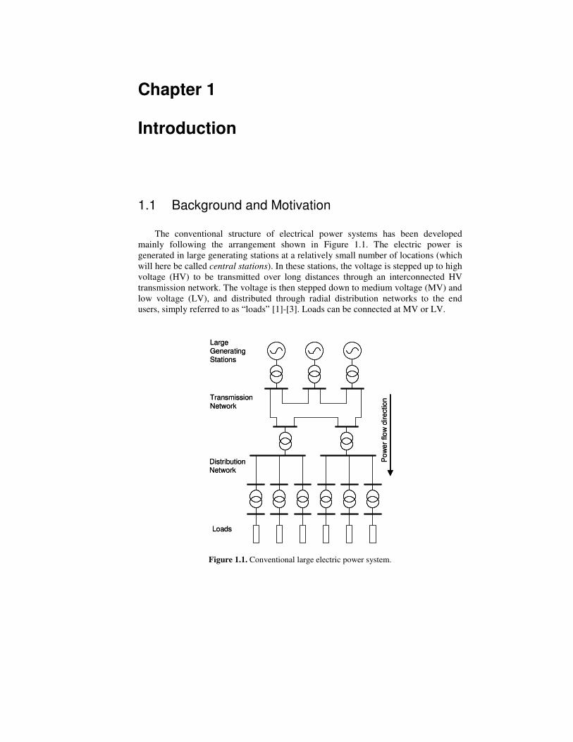
The conventional structure of electrical power systems has been developed mainly following the arrangement shown in Figure 1.1. The electric power is generated in large generating stations at a relatively small number of locations (which will here be called central stations). In these stations, the voltage is stepped up to high voltage (HV) to be transmitted over long distances through an interconnected HV transmission network. The voltage is then stepped down to medium voltage (MV) and low voltage (LV), and distributed through radial distribution networks to the end users, simply referred to as “loads” [1]-[3]. Loads can be connected at MV or LV.
LargeGeneratingStations
TransmissionNetwork
DistributionNetwork
Loads
Pow
er fl
ow d
irect
ion
LargeGeneratingStations
TransmissionNetwork
DistributionNetwork
Loads
Pow
er fl
ow d
irect
ion
Figure 1.1. Conventional large electric power system.
Chapter 1: Introduction
2
The conventional large electric power systems have existed for more than 50 years and improved through the years. These conventional systems offer a number of advantages [4]. Large generating units can be made efficient and operated with only a relatively small number of personnel. The interconnected high voltage transmission network allows generator reserve requirements to be minimized and the most efficient generating plant to be dispatched at any time, and bulk power can be transported over large distances with limited electrical losses. The distribution networks can be designed for unidirectional (radial) flows of power.
However, over the last few years, a number of factors have led to an increased interest in distributed generation schemes. According to the Kyoto Protocol, the EU has to reduce emissions of greenhouse gasses substantially to counter climate change [5]. The CIRED survey [6] asked representatives from 17 countries what the policy drivers are encouraging distributed generation. The answers include:
• reduction in gaseous emissions (mainly CO2); • energy efficiency or rational use of energy; • deregulation or competition energy; • diversification of energy resources; • national power requirements.
The CIGRE report [7], [8] listed similar reasons but with additional emphasis on commercial considerations, such as:
• availability of modular generating plant; • ease of finding sites for smaller generators; • short construction time and lower capital costs for smaller plant; • generation may be sited closer to load, which may reduce transmission costs. Hence most governments have programs to support the exploitation of so-called
new renewable energy resources. As renewable energy sources have a much lower energy density than fossil fuels, the generation plants are smaller and geographically spread.
Many terms and definitions are used to designate a small and geographically spread generation [9]. In this thesis distributed generation (DG) is defined according to [10], i.e. DG is any small-scale electrical power generation technology that provides electric power at or near the load site; it is either interconnected to the distribution system, directly to the customer’s facilities, or both. DG technologies considered in this thesis include internal combustion engines, small gas turbines, microturbines, small combined cycle gas turbines, microturbines, solar photovoltaic, fuel cells, and biomass, as considered in [10]-[11]. Geothermal and wind power are considered as DG when they are connected to the distribution system.
DG is gaining more and more attention worldwide as an alternative to large-scale centralized generating stations. For instance, cumulative wind power capacity in the EU countries increased by 20% to 34,205 MW at the end of 2004, up from 28,567 MW at the end of 2003 [12]. UK has targeted that 10% of the electricity generation should come from renewable resources by 2010, and 20% by 2020 [13]. In Sweden, electricity generation from solid biomass increased steadily from 1200 MW in 1990 to about 1800 MW by 2001; in IEA countries, solar photovoltaic generation
3
experienced an annual growth rate of 29% between 1992 and 2001 and wind turbine generation experienced an annual growth rate of 22.2% between 1990 and 2001 [14]. Indeed, the available data do not inform how many of those winds and renewable energy are connected to the distribution systems. However, those numbers indicate how DG is gaining attention.
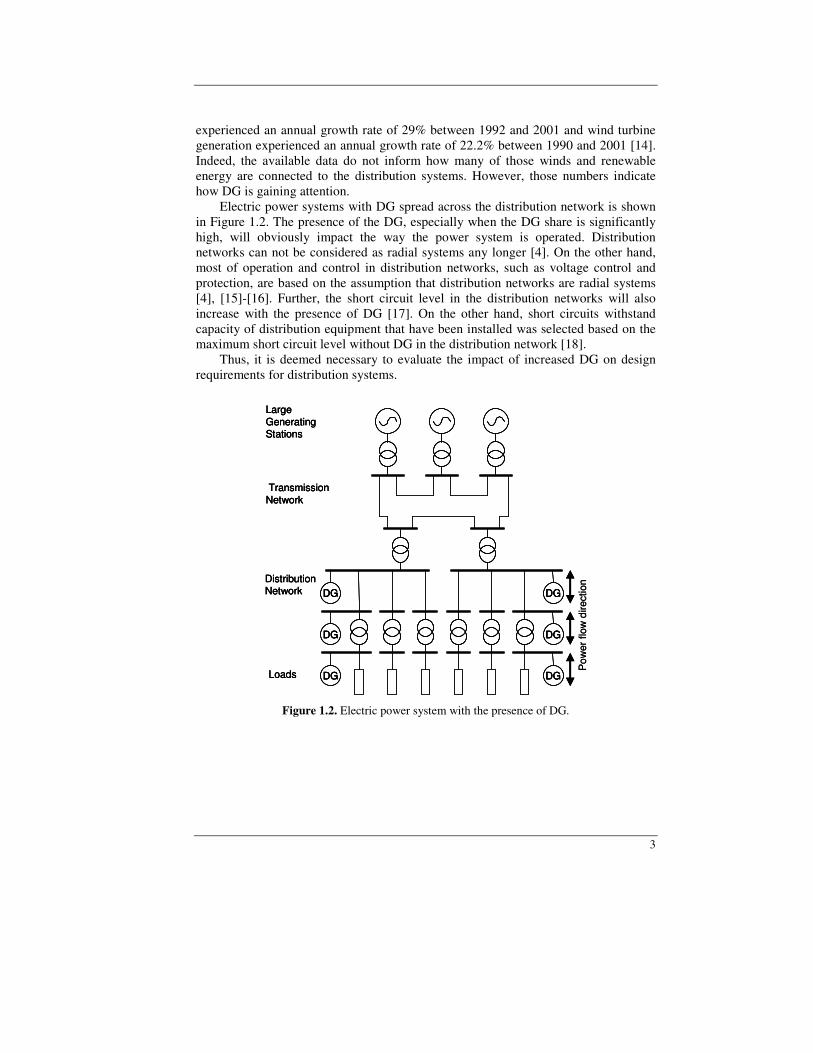
Electric power systems with DG spread across the distribution network is shown in Figure 1.2. The presence of the DG, especially when the DG share is significantly high, will obviously impact the way the power system is operated. Distribution networks can not be considered as radial systems any longer [4]. On the other hand, most of operation and control in distribution networks, such as voltage control and protection, are based on the assumption that distribution networks are radial systems [4], [15]-[16]. Further, the short circuit level in the distribution networks will also increase with the presence of DG [17]. On the other hand, short circuits withstand capacity of distribution equipment that have been installed was selected based on the maximum short circuit level without DG in the distribution network [18].
Thus, it is deemed necessary to evaluate the impact of increased DG on design requirements for distribution systems.
LargeGeneratingStations
TransmissionNetwork
DistributionNetwork
Loads
DG
DG
DG
DG
DG
DGP
ower
flow
dire
ctio
n
LargeGeneratingStations
TransmissionNetwork
DistributionNetwork
Loads
DG
DG
DG
DG
DG
DG
LargeGeneratingStations
TransmissionNetwork
DistributionNetwork
Loads
DGDG
DGDG
DGDG
DGDG
DGDG
DGDGP
ower
flow
dire
ctio
n
Figure 1.2. Electric power system with the presence of DG.
Chapter 1: Introduction
4
1.2 Aim and Outline of the Thesis
The aim of the thesis is to evaluate the impact of the DG to the steady state design and operation requirements for the distribution system. The emphasis is on voltage control, voltage dip and protection in the distribution system.
The thesis starts with an overview of DG in Chapter 2. Different DG technologies are treated briefly.
Chapter 3 presents the consequences of DG on voltage control in a LV feeder. Voltage control by controlling reactive power absorbed by the DG is presented as the solution to mitigate voltage control problems in a LV feeder with DG.
Chapter 4 discusses DG impact on voltage control in a LV feeder when DG power and load are varying stochastically. The selection of DG rating when taking into account the uncertainty of DG and load power, particularly in the case of solar photovoltaic generation, is presented.
Chapter 5 analyses voltage control in MV feeders with the presence of DG. Different mitigation methods to keep the voltage variation within allowed limits and their impacts are presented and compared.
Chapter 6 investigates the impact of DG on short circuit, voltage dip and overcurrent protection. The voltage dip study is extended to the coordination between voltage dip sensed by customers in a LV feeder and overcurrent protection in a MV feeder.
Chapter 7 proposes protection scheme for distribution systems with a high penetration of DG. The chapter starts with an overview of protection and control practices in transmission lines. The proposed scheme utilizes integrated microprocessor relays, which are normally used for high-speed protection and control of transmission lines.
Finally, conclusions and recommendations for future works are presented in Chapter 8.

Chapter 2
Distributed Generation Technology DG is based on different technologies, which are characterized by the source of energy. This chapter presents those DG technologies. The points that will be addressed such as: their potentials, challenges, typical sizes and ability to control their power output.
2.1 Introduction
DG produces electricity at a small scale at or near the load site. This approach is not likely to be used to replace central station plants, but it could respond to particular needs within competitive markets. However, many observers predict an increasing share of distributed generation in competitive electricity markets. Possible growth applications for distributed generation are [19]:
• industrial co-generation • support for network operation (provision of ancillary services) • insurance against power outages (standby power) • avoidance of high electricity prices during periods of peak demand • overcoming power transmission bottlenecks • applications requiring high power quality
The real potential for DG is difficult to assess, but any growth will be based on
the ability of small generating units to beat central station economy of scale, including transmission costs. A number of DG technologies are in a position to compete with central-station generation. Industrial co-generation is probably the largest potential area of growth for DG. Gas turbines, small Combine Cycle Gas Turbines (CCGTs), and industrial combustion engines have already proven their merit in industrial co-generation applications. Turbine and engine manufacturers have been intensifying their efforts to produce small, economic generation packages for DG [20]-[21].
There are likely to be opportunities for renewable energy technologies in DG. Remote sites with limited or no access to a central transmission network can sometimes take advantage of renewable energy sources because of the high cost of fossil fuel transport or of extending transmission lines. Indeed some renewable based
Chapter 2: Distributed Generation Technology
6
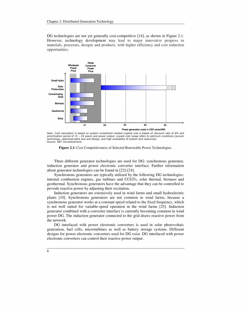
DG technologies are not yet generally cost-competitive [14], as shown in Figure 2.1. However, technology development may lead to major innovative progress in materials, processes, designs and products, with higher efficiency and cost reduction opportunities.
Wind
Geothermal
Biomass
Concentrating Solar
Solar Photovoltaic
Small Hydro
WholesalePowerPrice
RetailConsumer
PowerPrice
Power generation costs in USD cents/kWh
10 20 30 40 50
Wind
Geothermal
Biomass
Concentrating Solar
Solar Photovoltaic
Small Hydro
WholesalePowerPrice
RetailConsumer
PowerPrice
Power generation costs in USD cents/kWh
10 20 30 40 50
!" #
$#% #%$ #$ !&'("!& !
Figure 2.1: Cost Competitiveness of Selected Renewable Power Technologies. Three different generator technologies are used for DG: synchronous generator,
induction generator and power electronic converter interface. Further information about generator technologies can be found in [22]-[24].
Synchronous generators are typically utilized by the following DG technologies: internal combustion engines, gas turbines and CCGTs, solar thermal, biomass and geothermal. Synchronous generators have the advantage that they can be controlled to provide reactive power by adjusting their excitation.
Induction generators are extensively used in wind farms and small hydroelectric plants [10]. Synchronous generators are not common in wind farms, because a synchronous generator works at a constant speed related to the fixed frequency, which is not well suited for variable-speed operation in the wind farms [25]. Induction generator combined with a converter interface is currently becoming common in wind power DG. The induction generator connected to the grid draws reactive power from the network.
DG interfaced with power electronic converters is used in solar photovoltaic generation, fuel cells, microturbines as well as battery storage systems. Different designs for power electronic converters used for DG exist. DG interfaced with power electronic converters can control their reactive power output.
7
DG technology is characterized by the energy source of the DG, which will be discussed briefly in the following sections. Further information can be read in [10]-[11], [19], [26]-[28].
2.2 Internal Combustion Engines
Reciprocating internal combustion engines (ICEs) convert heat from combustion of a fuel into rotary motion which, in turn, drives a generator in a distributed generation (DG) system.
ICEs are the most common technology used for DG [10]-[11]. They are a proven technology with low capital cost; large size range, from a few kW to MW; good efficiency; possible thermal or electrical cogeneration in buildings and good operating reliability. These characteristics, combined with the engines’ ability to start up fast during a power outage, make them the main choice for emergency or standby power supplies.
The key barriers to ICE usage are: high maintenance cost, which is the highest among the DG technologies; high NOX emissions, which are also highest among the DG technologies and a high noise level.
2.3 Gas Turbines
Gas turbines consist of a compressor, combustor, and turbine-generator assembly that converts the rotational energy into electrical power output.
Gas turbines of all sizes are now widely used in the power industry. Small industrial gas turbines of 1 – 20 MW are commonly used in CHP applications [11]. They are particularly useful when higher temperature steam is required than can be produced by a reciprocating engine. The maintenance cost is slightly lower than for reciprocating engines.
Gas turbines can be noisy. Emissions are somewhat lower than for combustion engines, and cost-effective NOX emissions-control technology is commercially available.
2.4 Combined Cycle Gas Turbines
In a CCGT, the exhaust air–fuel mixture exchanges energy with water in the boiler to produce steam for the steam turbine. The steam enters the steam turbine and
Chapter 2: Distributed Generation Technology
8
expands to produce shaft work, which is converted into additional electric energy in the generator. Finally, the outlet flow from the turbine is condensed and returned to the boiler. The CCGT is becoming increasingly popular due to its high efficiency. However, GT installations below 10 MW are generally not combined-cycle, due to the scaling inefficiencies of the steam turbine [10].
2.5 Microturbines
Microturbines extend gas-turbine technology to smaller scales. The technology was originally developed for transportation applications, but is now finding a niche in power generation. One of the most striking technical characteristics of microturbines is their extremely high rotational speed. The turbine rotates up to 120 000 rpm and the generator up to 40 000 rpm. Microturbines produce high frequency ac power. Power electronic inverter converts this high frequency power into a usable form.
Individual unit of microturbines ranges from 30 - 200 kW but can be combined readily into systems of multiple units [11]. Low combustion temperatures can assure very low NOX emissions levels. They make much less noise than an engine of comparable size.
The main disadvantages of microturbines at the moment are its short track record and high costs compared with gas combustion engines.
2.6 Fuel Cells
Fuel cells are electrochemical devices that convert the chemical energy of a fuel directly to usable energy — electricity and heat — without combustion. This is quite different from most electric generating devices (e.g., steam turbines, gas turbines, and combustion engines) which first convert the chemical energy of a fuel to thermal energy, then to mechanical energy, and, finally, to electricity.
Fuel cells produce electricity with high efficiencies, 40 to 60%, with negligible harmful emissions, and operate so quietly that they can be used in residential neighborhoods. These are the main advantages of fuel cells, besides their scalability and modularity. The Individual module of a fuel cell can range from 1 kW to 5 MW [9].
The main challenge to make fuel cells widely used in the DG market is to make fuel cells more economically competitive with current technologies.

9
2.7 Solar Photovoltaic Photovoltaic (PV) systems involve the direct conversion of sunlight into
electricity without heat engine. PV systems have been used as the power sources for calculators, watches, water
pumping, remote buildings, communications, satellites and space vehicles, as well as megawatt-scale power plants.
As indicated in Figure 2.1, PV systems are expensive. Without subsidies, PV power remains two to five times as expensive as grid power, where grid power exists. However, where there is no grid, PV power is the cheapest electricity source, when operating and maintenance costs are considered. PV systems can also be competitive to supply load during peak demand period, where the peaking power is sold at high multiples of the average cost.
The attractive features of PV systems are modularity, easy maintainability, low weight, very low operation cost, environmental benignness and their ability for off-grid application. Mostly, individual range of PV module ranges from 20 Watt to 100 kW [9]. Several barriers for PV systems include significant area requirements due to the diffuse nature of the solar resource, higher installation cost than other DG technologies, and intermittent output with a low load factor [10]-[11].
2.8 Solar Thermal (Concentrating Solar)
Solar thermal systems use solar radiation for a heat engine to generate electricity. Applications of concentrating solar power are now feasible from a few kilowatts to hundreds of megawatts. Solar-thermal plants can function in dispatchable, grid-connected markets or in distributed, stand-alone applications. They are suitable for fossil-hybrid operation or can include cost-effective thermal storage to meet dispatchability requirements [25].
Moreover, they can operate worldwide in regions having high direct normal insolation, including large areas of Africa, Australia, China, India, the Mediterranean region, the Middle East, the South-western United States, and Central and South America. “High direct normal insolation” means strong sunlight where the atmosphere contains little water vapour, which tends to diffuse the light.

Chapter 2: Distributed Generation Technology
10
2.9 Wind Power The use of wind energy dates back many centuries, perhaps even thousands of
years. The step from mechanical to electrical use of wind energy was made in the USA. In 1888, Charles F. Brush developed an automatically operating wind machine performing at a rated power of 12 kW dc. Small-scale stand-alone systems continued to be the main focus of wind power applications for another five decades. The first ac turbine was built in the 1930s in the USA. At first, further use of wind power suffered from the less expensive grid power but interest in wind energy grew through energy emergencies such as World War II and the oil crisis in the early 1970s. The development of modern wind power machines has been led by Denmark, Germany, the Netherlands, Spain, and the USA. Through these developments, wind power has become an important electricity option for large-scale on-grid use [25].
Today, large wind-power plants are competing with electric utilities in supplying economical clean power in many parts of the world [27]. In this sense, wind power is more like central generation than distributed generation. The average turbine size of the wind installations has increased significantly from 20 kW in 1985 to be 1.4 MW in 2002 [14], as shown in Figure 2.2, which creates an economic of scale for the wind technology.
Figure 2.2: Average Wind Turbine Size at Market Introduction
However, wind power generation faces some challenges for future growth. The main challenges are intermittency and grid reliability [14]. Since wind power generation is based on natural forces, it cannot dispatch power on demand. On the other hand, utilities must supply power in close balance to demand. Thus, as the share of wind energy increases, integration of wind turbines into the electrical network will need both more attention and investment. Another barrier is transmission availability.
11
This is because, sometimes, the best locations for wind farms are in remote area without close access to a transmission line.
2.10 Small Hydropower
Hydropower turbines were first used to generate electricity for large scale use was in the 1880s [25]. Expansion and increasing access to transmission networks had led to concentrating power generation in large units benefiting from economies of scale. This resulted in a trend of building large hydropower installations rather than small hydropower systems for several decades. However, liberalization of the electricity industry has contributed in some areas to the development of hydropower generating capacity by independent power producers (IPPs).
There is no international consensus on the definition of small hydropower. However, common definitions for small hydropower electric facilities are [14], [25]:
• Small hydropower: capacity of less than 10 MW. • Mini hydropower: capacity between 100 kW and 1 MW. • Micro hydropower: capacity below 100 kW.
2.11 Geothermal
Geothermal is energy available as heat emitted from within the earth, usually in the form of hot water or steam. Geothermal as a recoverable energy resource is very site specific. Geothermal power plant can range from hundreds kW to hundreds MW [25].

Chapter 2: Distributed Generation Technology
12
Chapter 3
Voltage Control on Low Voltage Feeder
with Distributed Generation
This chapter discusses voltage control in a LV feeder with DG. The chapter starts with two calculation methods. It then continues with an overview of voltage increase due to the DG and voltage rise mitigation by DG operation at a leading power factor. The impact of DG and voltage rise mitigation on feeder losses is investigated further. Simplified expressions of DG active power that will give loss minimization or unchanged losses are derived.
3.1 Introduction Steady-state voltage in distribution networks can be controlled in several ways. The most popular voltage control equipment includes on-load tap changer on substation transformer, capacitor bank and line voltage regulator, which are mostly used in MV networks [2]. On the other hand, off-load tap changer on distribution transformer can be used to adjust the voltage at the LV side. One of voltage control objectives is to keep the voltage at the customer within a suitable range during normal operation. The voltage range for normal operation is defined in different standards. IEEE Std. 1159-1995 and CENELEC EN 50160 indicate + 10% voltage variation (from the nominal voltage) as normal operating voltage [29]-[30]. The Swedish Standard SS 421-18-11 indicates +6%/-10% voltage variations as normal operating voltage. Voltage control equipment were designed and operated based on a planned centralized generation and on the assumption that the current always flows from the substation to the MV system, and then to LV customers; and that the voltage decreases towards the end of the feeder. The introduction of DG makes this assumption no longer valid. DG generally will increase voltage at its connection point, which may cause overvoltage during low load conditions [4],[31]. The effect of a single DG on the voltage profile of a LV distribution feeder was analyzed in [32], by assuming that the line reactance is negligible. However, the reactance of overhead (OH) lines in a LV feeder is in the same order as the resistance. This indicates that the reactance should not be neglected.
Chapter 3: Voltage Control on LV Feeder with DG
14
When the contribution of DG power is high; DG may cause either the voltage to exceed maximum allowed voltage Umax, or the reverse current (from the DG to the source) exceeds the thermal ampacity of the conductor Imax, or the reverse power exceeds the rating of distribution transformer STX [31],[33]. Maximum power that DG can generate without violating Umax, Imax and STX is here referred to as the DG integration limit and denoted as PDG,max. The voltage rise due to DG can be deferred by DG absorbs reactive power from the grid [31],[33]. When DG is operated at unity pf, Umax will most probably be reached earlier, except when the location of DG is very close to the source (MV/LV transformer). Consequently, reactive power absorption, when it is limited by Umax, will probably extend the DG integration limit. A linear approximation is commonly used to calculate voltage rise due to DG, as in [34]-[36]. The calculation may be correct when the DG power source is only small. However, when the approximation is used to find the DG integration limit, further assessment is needed to ensure that the calculations yield correct numbers. It has been mentioned in many papers that DG offers loss reduction benefits. However, this benefit cannot be taken for granted [17],[37]. Moreover, reactive power absorption will likely cause an increase in losses. Detailed investigations are needed to ensure whether the DG decreases or increases the feeder losses.
3.2 Voltage Drop Calculation Methods
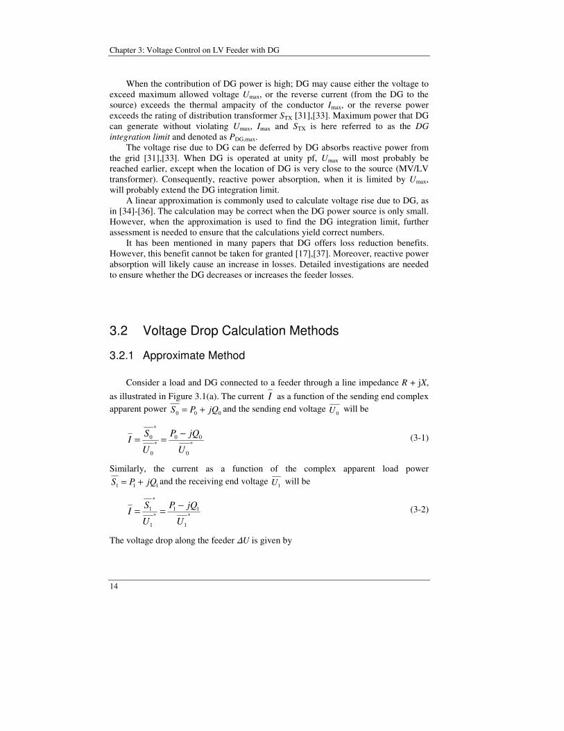
3.2.1 Approximate Method Consider a load and DG connected to a feeder through a line impedance R + jX, as illustrated in Figure 3.1(a). The current I as a function of the sending end complex apparent power 000 jQPS += and the sending end voltage
0U will be
*
0
00*
0
*
0
U
jQP
U
SI
−== (3-1)
Similarly, the current as a function of the complex apparent load power
111 jQPS += and the receiving end voltage 1U will be
*
1
11*
1
*
1
U
jQP
U
SI
−== (3-2)
The voltage drop along the feeder U is given by
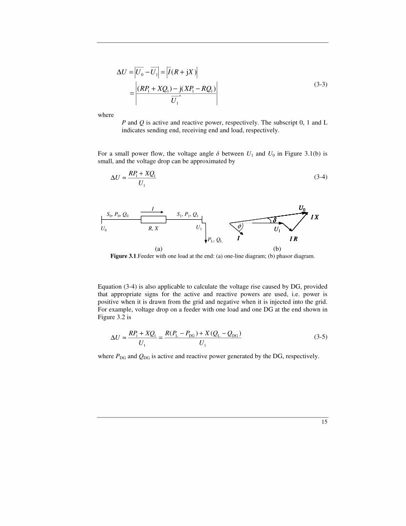
15
*
1
1111
10
)(j)(
)j(
U
RQXPXQRP
XRIUUU
−−+=
+=−=∆
(3-3)
where P and Q is active and reactive power, respectively. The subscript 0, 1 and L indicates sending end, receiving end and load, respectively.
For a small power flow, the voltage angle between U1 and U0 in Figure 3.1(b) is small, and the voltage drop can be approximated by
1
11
UXQRP
U+≈∆ (3-4)
U0
IS1, P1, Q1S0, P0, Q0
R, X U1
PL, QL
δU1
U0
I R
I X
I
φδ
U0
I R
I X
I
φδU1
U0
I R
I X
I
φδ
U0
I R
I X
I
φ
(a) (b)
Figure 3.1.Feeder with one load at the end: (a) one-line diagram; (b) phasor diagram.
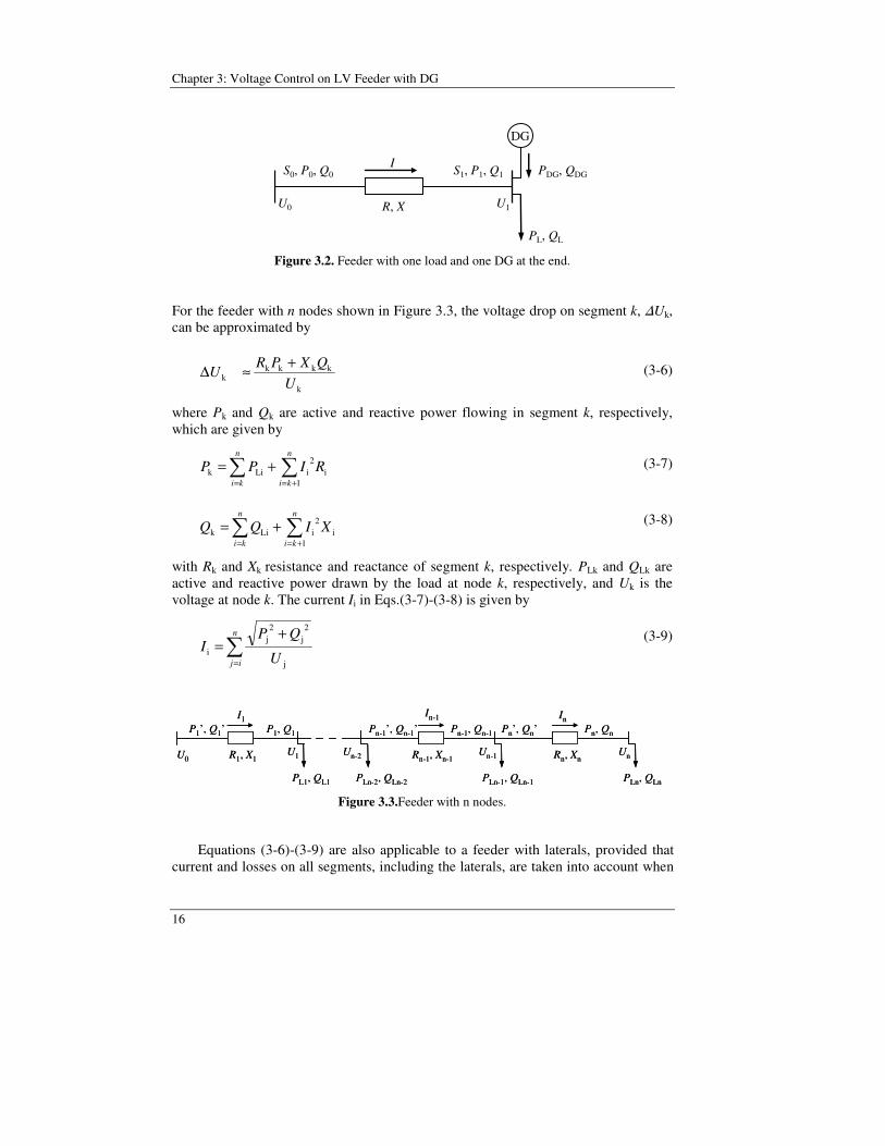
Equation (3-4) is also applicable to calculate the voltage rise caused by DG, provided that appropriate signs for the active and reactive powers are used, i.e. power is positive when it is drawn from the grid and negative when it is injected into the grid. For example, voltage drop on a feeder with one load and one DG at the end shown in Figure 3.2 is
1
DGLDGL
1
11 )()(U
QQXPPRU
XQRPU
−+−=+≈∆ (3-5)
where PDG and QDG is active and reactive power generated by the DG, respectively.
Chapter 3: Voltage Control on LV Feeder with DG
16
U0
I S1, P1, Q1S0, P0, Q0
U1
PL, QL
R, X
DG
PDG, QDG
Figure 3.2. Feeder with one load and one DG at the end.
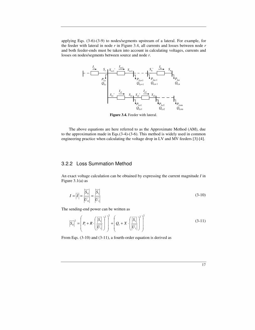
For the feeder with n nodes shown in Figure 3.3, the voltage drop on segment k, Uk, can be approximated by
k
kkkkk U
QXPRU
+≈∆ (3-6)
where Pk and Qk are active and reactive power flowing in segment k, respectively, which are given by
= +=
+=n
ki
n
ki
RIPP1
i2
iLik (3-7)
= +=
+=n
ki
n
ki
XIQQ1
i2
iLik (3-8)
with Rk and Xk resistance and reactance of segment k, respectively. PLk and QLk are active and reactive power drawn by the load at node k, respectively, and Uk is the voltage at node k. The current Ii in Eqs.(3-7)-(3-8) is given by
=
+=
n
ij U
QPI
j
2j
2j
i (3-9)
U0
I1P1, Q1P1’, Q1’
R1, X1U1
PL1, QL1
In-1
Pn-1, Qn-1Pn-1’, Qn-1’
Rn-1, Xn-1Un-1
PLn-1, QLn-1
Un-2
PLn-2, QLn-2
InPn, QnPn’, Qn’
Rn, XnUn
PLn, QLn
U0
I1P1, Q1P1’, Q1’
R1, X1U1
PL1, QL1
In-1
Pn-1, Qn-1Pn-1’, Qn-1’
Rn-1, Xn-1Un-1
PLn-1, QLn-1
Un-2
PLn-2, QLn-2
InPn, QnPn’, Qn’
Rn, XnUn
PLn, QLn Figure 3.3.Feeder with n nodes.
Equations (3-6)-(3-9) are also applicable to a feeder with laterals, provided that current and losses on all segments, including the laterals, are taken into account when
17
applying Eqs. (3-6)-(3-9) to nodes/segments upstream of a lateral. For example, for the feeder with lateral in node r in Figure 3.4, all currents and losses between node r and both feeder-ends must be taken into account in calculating voltages, currents and losses on nodes/segments between source and node r.
PLrQLr
PLn-1QLn-1
PLnQLn
Sn’In Sn
PLr+1QLr+1
Ir Sr Sr+1’Ir+1
Sr+1
PLr1QLr1
Ir1Sr1Sr1’
PLr2QLr2
Ir2Sr2Sr2’
PLrmQLrm
Figure 3.4. Feeder with lateral.
The above equations are here referred to as the Approximate Method (AM), due to the approximation made in Eqs.(3-4)-(3-6). This method is widely used in common engineering practice when calculating the voltage drop in LV and MV feeders [3]-[4].
3.2.2 Loss Summation Method An exact voltage calculation can be obtained by expressing the current magnitude I in Figure 3.1(a) as
1
1
0
0
U
S
U
SII === (3-10)
The sending-end power can be written as
22
1
1
1
22
1
1
1
2
0
⋅++
⋅+=
U
SXQ
U
SRPS (3-11)
From Eqs. (3-10) and (3-11), a fourth-order equation is derived as
Chapter 3: Voltage Control on LV Feeder with DG
18
0
2
1
1
22
1
1 =+
+
C
U
SB
U
SA (3-12)
Where
21
21
2011
22
22
QPC
UXQRPB
XRA
+=
−+=
+=
The current magnitude I can be derived from (3-10) as
1
21
21
U
QPI
+= (3-13)
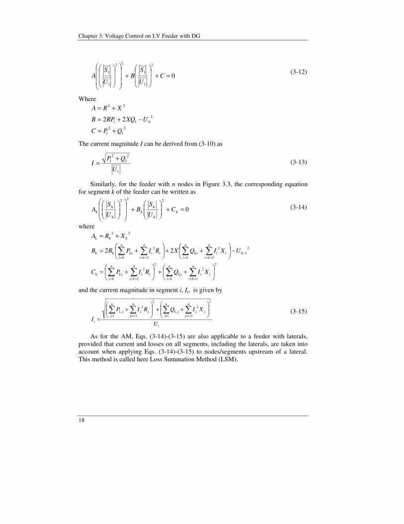
Similarly, for the feeder with n nodes in Figure 3.3, the corresponding equation for segment k of the feeder can be written as
0k
2
k
kk
22
k
kk =+
+
C
U
SB
U
SA (3-14)
where
2
1i
2iLi
2
1i
2iLik
21k
1i
2iLi
1i
2iLikk
2k
2kk
22
++
+=
−
++
+=
+=
= +== +=
−= +== +=
n
ki
n
ki
n
ki
n
ki
n
ki
n
ki
n
ki
n
ki
XIQRIPC
UXIQXRIPRB
XRA
and the current magnitude in segment i, Ii, is given by
i
2n
ij
n
1ijj
2jjL,
2n
ij
n
1ijj
2jjL,
i U
XIQRIP
I
++
+
=
= +== += (3-15)
As for the AM, Eqs. (3-14)-(3-15) are also applicable to a feeder with laterals, provided that current and losses on all segments, including the laterals, are taken into account when applying Eqs. (3-14)-(3-15) to nodes/segments upstream of a lateral. This method is called here Loss Summation Method (LSM).
19
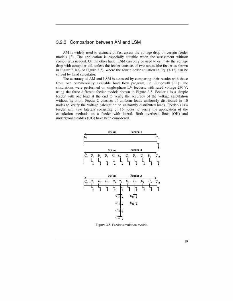
3.2.3 Comparison between AM and LSM AM is widely used to estimate or fast assess the voltage drop on certain feeder models [3]. The application is especially suitable when the assessment without computer is needed. On the other hand, LSM can only be used to estimate the voltage drop with computer aid, unless the feeder consists of two nodes (the feeder as shown in Figure 3.1(a) or Figure 3.2), where the fourth order equation in Eq. (3-12) can be solved by hand calculator. The accuracy of AM and LSM is assessed by comparing their results with those from one commercially available load flow program, i.e. Simpow® [38]. The simulations were performed on single-phase LV feeders, with rated voltage 230 V, using the three different feeder models shown in Figure 3.5. Feeder-1 is a simple feeder with one load at the end to verify the accuracy of the voltage calculation without iteration. Feeder-2 consists of uniform loads uniformly distributed in 10 nodes to verify the voltage calculation on uniformly distributed loads. Feeder-3 is a feeder with two laterals consisting of 16 nodes to verify the application of the calculation methods on a feeder with lateral. Both overhead lines (OH) and underground cables (UG) have been considered.
Feeder-2
U10
0.5 km Feeder-1
U0
Feeder-3
U0 U10
U1
U1 U2 U5 U7U3 U4 U6 U9U8
U11
U16
U12U14
U15
U13
0.5 km
0.5 km
U0 U1 U2 U5 U7U3 U4 U6 U9U8
Feeder-2
U10
0.5 km Feeder-1
U0
Feeder-3
U0 U10
U1
U1 U2 U5 U7U3 U4 U6 U9U8
U11
U16
U12U14
U15
U13
0.5 km
0.5 km
U0 U1 U2 U5 U7U3 U4 U6 U9U8
Figure 3.5. Feeder simulation models.
Chapter 3: Voltage Control on LV Feeder with DG
20
Conductor parameters (resistance per km r, reactance per km x and ampacity Imax) shown in Table 3.1 have been adapted by the author based on information from [39]-[41]. The load power factor (pfL) was varied between 1.0 and 0.7 (lagging). It is assumed that the secondary voltage of the MV/LV transformer is 1.0 pu, which will be held throughout this chapter. The simulation results pu will be equally valid for three phase feeders.
TABLE 3.1
CONDUCTOR PARAMETERS FOR LV FEEDER SIMULATION
Overhead line (OH) Underground cable (UG) Size (mm2) r (Ω/km) x (Ω/km) Imax (A) r (Ω/km) x (Ω/km) Imax (A)
16 1.10 0.32 150 1.15 0.11 115 70 0.27 0.27 360 0.27 0.095 260
160 0.12 0.25 610 0.12 0.09 400
Voltage drop simulation using both AM and LSM and their comparison with Simpow simulation for feeder-1 is shown in Figure 3.6. The simulations were performed by increasing the load power until maximum load PL,max is reached by the AM. PL,max is the load that causes either the conductor ampacity Imax or the minimum allowed voltage Umin to be reached. Umin is taken as 0.90 pu as defined by standards presented in Section 3.1. Figure 3.6 indicates that the accuracy of AM decreases with the increase of load, and the increase of pf. This can intuitively be concluded from Eqs. (3-3)-(3-4), i.e.: error will increase with the increase of P, meanwhile RQ counteracts the error caused by XP. On the other hand, LSM, which is still simple for this two-node feeder (hand calculation is still possible), always yields accurate results. The accuracy of voltage drop calculation with AM was also found to be affected by the type of conductor used, as can be seen in Figure 3.7 - Figure 3.8. For the same active power drawn by the load, the error will be approximately the same for the three OH lines, as those conductors have almost the same reactance. The same is true thing for the three UG cables. On the other hand, for the same active power drawn by the load, UG cables give better accuracy. All of those can intuitively be observed from Eqs. (3-3)-(3-4); i.e. when there is no reactive power drawn by the loads, the error will increase with the increase of PX.

21
pfL = 1.0
pfL = 0.95
pfL = 0.70
pfL = 0.85
pfL = 1.0
pfL = 0.95
pfL = 0.70
pfL = 0.85
Figure 3.6. Voltage at the end of for feeder-1 as function of load power for different values of pf with AM and LSM. The conductor used is 160 mm2 OH in Table 3.1.
The markers “”, “”,“”, and “” indicate results from Simpow. These markers will be used thorough this Chapter.
160 mm2 OH
70 mm2 OH16 mm2 OH
160 mm2 OH
70 mm2 OH16 mm2 OH
Figure 3.7. Comparison between AM and LSM in the calculation of the voltage at the end of
for feeder-1, when different OH lines are used. Loads have unity power factor.

Chapter 3: Voltage Control on LV Feeder with DG
22
160 mm2 UG
70 mm2 UG16 mm2 UG
Figure 3.8. Comparison between AM and LSM in the calculation of the voltage at the end of
feeder-1, when different UG cables are used. Loads have unity power factor.
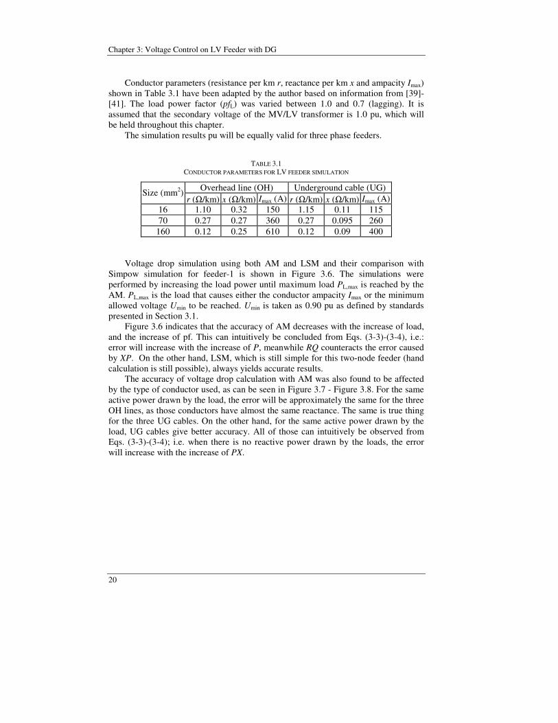
Voltage drop simulation for feeder-2 is shown in Figure 3.9. The figure indicates that both AM and LSM are accurate to calculate the voltage drop on the feeder with many nodes. Accordingly, further simulations (not shown) also indicate that both AM and LSM are also accurate to calculate voltage drop on feeder-3 for any loads lower than PL,max. As in case of feeder-1; the accuracy is even better when UG cables are used (not shown here). Thus, AM is considerably accurate to calculate the voltage drop on the feeder with many nodes. However, it should be noted that the application of AM in this case requires iterative calculation, as shown in Eqs.(3-6)-(3-9), as it is needed in LSM. This means that computer aid is still needed. Calculation by hand is still possible when the loads are uniformly distributed and the feeder has no laterals [3], at the expense of less accuracy, especially when the number of load nodes is not big enough. The voltage at the end of the feeder as a function of DG power when DG is connected at the end of feeder-1 is shown in Figure 3.10. The simulations were performed by increasing the load power until DG integration limit PDG,max is reached. Umax is taken as 1.06 pu as defined by the strictest standard presented in Section 3.1.
23
pfL = 1.0
pfL = 0.95
pfL = 0.70
pfL = 0.85
pfL = 1.0
pfL = 0.95
pfL = 0.70
pfL = 0.85
Figure 3.9. Voltage at the end of for feeder-2 as function of load power for different values of
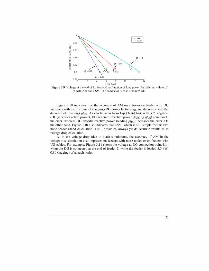
pf with AM and LSM. The conductor used is 160 mm2 OH. Figure 3.10 indicates that the accuracy of AM on a two-node feeder with DG increases with the decrease of (lagging) DG power factor pfDG, and decreases with the decrease of (leading) pfDG. As can be seen from Eqs.(3-3)-(3-4), with XP1 negative (DG generates active power), DG generates reactive power (lagging pfDG) counteracts the error, whereas DG absorbs reactive power (leading pfDG) increases the error. On the other hand, Figure 3.10 also indicates that LSM, which is still simple for this two node feeder (hand calculation is still possible), always yields accurate results as in voltage drop calculation. As in the voltage drop (due to load) simulations, the accuracy of AM in the voltage rise simulation also improves on feeders with more nodes or on feeders with UG cables. For example, Figure 3.11 shows the voltage at DG connection point UDG when the DG is connected at the end of feeder-2, while the feeder is loaded 5.5 kW, 0.80 (lagging) pf at each nodes.

Chapter 3: Voltage Control on LV Feeder with DG
24
pfDG = 1.0
pfDG = 0.99
pfDG = 0.98
pfDG = 1.0
pfDG = 0.99
pfDG = 0.98
pfDG = 1.0
pfDG = 0.99
pfDG = 0.98
pfDG = 1.0
pfDG = -0.99
pfDG = -0.98
pfDG = 1.0
pfDG = -0.99
pfDG = -0.98
Figure 3.10. Voltage at the end of Feeder-1 as function of DG power for different values of
pfDG with AM and LSM, for lagging pfDG (top) and leading pfDG (bottom). No load is connected to the feeder. The conductor used is 160 mm2 OH.
Due to possible error caused by AM when the DG or load power is high and the better accuracy of LSM, LSM is used for the simulation in the remainder of this chapter, unless otherwise specified. However, AM is still used for analysis. Further, the simulation results are always verified against the results from Simpow, even when they are not shown in the plot.
25
pfDG = 1.0
pfDG = -0.99
pfDG = -0.98
pfDG = 1.0
pfDG = -0.99
pfDG = -0.98
Figure 3.11. Voltage at the end of for feeder-2 as function of DG power for different values of
pfDG with AM (left) and LSM (right). The conductor used is 160 mm2 OH.
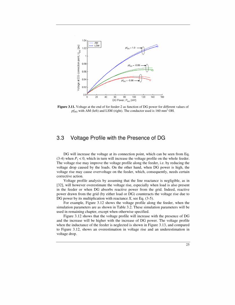
3.3 Voltage Profile with the Presence of DG DG will increase the voltage at its connection point, which can be seen from Eq. (3-4) when P1 < 0, which in turn will increase the voltage profile on the whole feeder. The voltage rise may improve the voltage profile along the feeder, i.e. by reducing the voltage drop caused by the loads. On the other hand, when DG power is high, the voltage rise may cause overvoltage on the feeder, which, consequently, needs certain corrective action. Voltage profile analysis by assuming that the line reactance is negligible, as in [32], will however overestimate the voltage rise, especially when load is also present in the feeder or when DG absorbs reactive power from the grid. Indeed, reactive power drawn from the grid (by either load or DG) counteracts the voltage rise due to DG power by its multiplication with reactance X, see Eq. (3-5). For example, Figure 3.12 shows the voltage profile along the feeder, when the simulation parameters are as shown in Table 3.2. These simulation parameters will be used in remaining chapter, except when otherwise specified. Figure 3.12 shows that the voltage profile will increase with the presence of DG and the increase will be higher with the increase of DG power. The voltage profile when the inductance of the feeder is neglected is shown in Figure 3.13, and compared to Figure 3.12, shows an overestimation in voltage rise and an underestimation in voltage drop.

Chapter 3: Voltage Control on LV Feeder with DG
26
TABLE 3.2 SIMULATION PARAMETERS
Feeder model : Feeder-2 Load power, PL : 3 kW at each node Load power factor, pfL : 0.85 lagging DG connection : Node-10 Conductor : 70 mm2
OH in Table 3.1
Figure 3.12. Voltage profile along Feeder-2 with and without DG. Simulation parameters are given in Table 3.2.
Figure 3.13. Voltage profile along Feeder-2 as the case in Figure 3.12 when line reactance is
neglected.
27
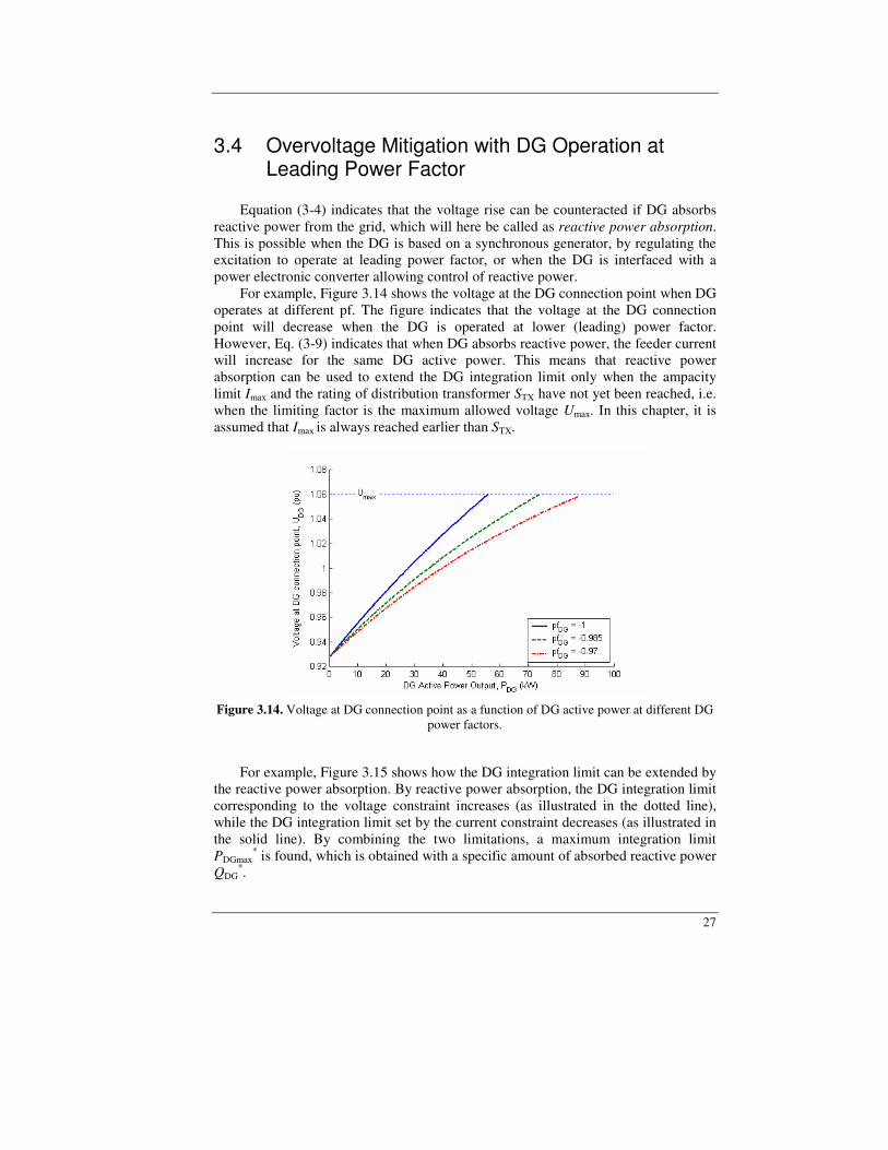
3.4 Overvoltage Mitigation with DG Operation at Leading Power Factor
Equation (3-4) indicates that the voltage rise can be counteracted if DG absorbs reactive power from the grid, which will here be called as reactive power absorption. This is possible when the DG is based on a synchronous generator, by regulating the excitation to operate at leading power factor, or when the DG is interfaced with a power electronic converter allowing control of reactive power. For example, Figure 3.14 shows the voltage at the DG connection point when DG operates at different pf. The figure indicates that the voltage at the DG connection point will decrease when the DG is operated at lower (leading) power factor. However, Eq. (3-9) indicates that when DG absorbs reactive power, the feeder current will increase for the same DG active power. This means that reactive power absorption can be used to extend the DG integration limit only when the ampacity limit Imax and the rating of distribution transformer STX have not yet been reached, i.e. when the limiting factor is the maximum allowed voltage Umax. In this chapter, it is assumed that Imax is always reached earlier than STX.
Figure 3.14. Voltage at DG connection point as a function of DG active power at different DG
power factors.
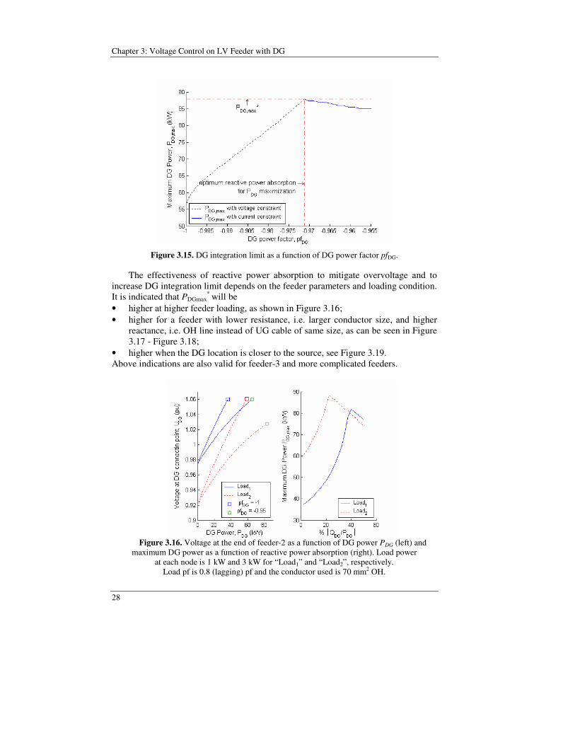
For example, Figure 3.15 shows how the DG integration limit can be extended by the reactive power absorption. By reactive power absorption, the DG integration limit corresponding to the voltage constraint increases (as illustrated in the dotted line), while the DG integration limit set by the current constraint decreases (as illustrated in the solid line). By combining the two limitations, a maximum integration limit PDGmax
* is found, which is obtained with a specific amount of absorbed reactive power QDG
*.
Chapter 3: Voltage Control on LV Feeder with DG
28
Figure 3.15. DG integration limit as a function of DG power factor pfDG.
The effectiveness of reactive power absorption to mitigate overvoltage and to
increase DG integration limit depends on the feeder parameters and loading condition. It is indicated that PDGmax
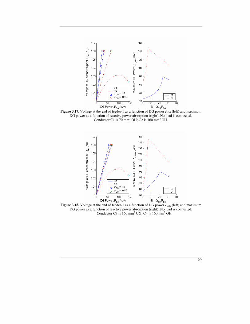
* will be • higher at higher feeder loading, as shown in Figure 3.16; • higher for a feeder with lower resistance, i.e. larger conductor size, and higher
reactance, i.e. OH line instead of UG cable of same size, as can be seen in Figure 3.17 - Figure 3.18;
• higher when the DG location is closer to the source, see Figure 3.19. Above indications are also valid for feeder-3 and more complicated feeders.
Figure 3.16. Voltage at the end of feeder-2 as a function of DG power PDG (left) and
maximum DG power as a function of reactive power absorption (right). Load power at each node is 1 kW and 3 kW for “Load1” and “Load2”, respectively.
Load pf is 0.8 (lagging) pf and the conductor used is 70 mm2 OH.
29
Figure 3.17. Voltage at the end of feeder-1 as a function of DG power PDG (left) and maximum
DG power as a function of reactive power absorption (right). No load is connected. Conductor C1 is 70 mm2 OH; C2 is 160 mm2 OH.
Figure 3.18. Voltage at the end of feeder-1 as a function of DG power PDG (left) and maximum
DG power as a function of reactive power absorption (right). No load is connected. Conductor C3 is 160 mm2 UG; C4 is 160 mm2 OH.
Chapter 3: Voltage Control on LV Feeder with DG
30
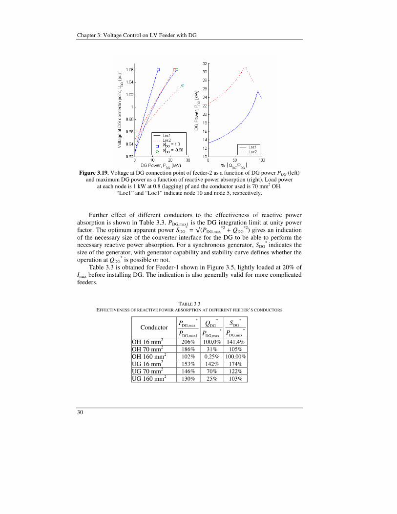
Figure 3.19. Voltage at DG connection point of feeder-2 as a function of DG power PDG (left)
and maximum DG power as a function of reactive power absorption (right). Load power at each node is 1 kW at 0.8 (lagging) pf and the conductor used is 70 mm2 OH.
“Loc1” and “Loc1” indicate node 10 and node 5, respectively. Further effect of different conductors to the effectiveness of reactive power
absorption is shown in Table 3.3. PDG,max1 is the DG integration limit at unity power factor. The optimum apparent power SDG
* = (PDG,max*2 + QDG
*2) gives an indication of the necessary size of the converter interface for the DG to be able to perform the necessary reactive power absorption. For a synchronous generator, SDG
* indicates the size of the generator, with generator capability and stability curve defines whether the operation at QDG
* is possible or not. Table 3.3 is obtained for Feeder-1 shown in Figure 3.5, lightly loaded at 20% of
Imax before installing DG. The indication is also generally valid for more complicated feeders.
TABLE 3.3 EFFECTIVENESS OF REACTIVE POWER ABSORPTION AT DIFFERENT FEEDER’S CONDUCTORS
Conductor max1DG,
*maxDG,
P
P *
maxDG,
*DG
PQ
*maxDG,
*DG
PS
OH 16 mm2 206% 100,0% 141,4% OH 70 mm2 186% 31% 105% OH 160 mm2
2102% 0,25% 100,00%
UG 16 mm2 153% 142% 174% UG 70 mm2 146% 70% 122% UG 160 mm2 130% 25% 103%

31
It can be seen from Table 3.3 that the DG integration limit increases greatly with the reactive power absorption for OH line. The increase is more contained for UG cable. Moreover, the DG integration limit increases more for lower size of conductor (both for OH and UG). Note however that the reactive power absorption necessary to achieve the maximum integration limit can be very high for a small conductor. For example, the size of the converter must be 1.4 times the size of the generator for OH line with 16 mm2 conductor. In comparison, for a OH line with 70 mm2 conductor, the injected active power can be increased by 86% with the size of converter 105% of the generator.
3.5 Voltage Control with DG and its Impact on Losses DG may reduce the current flowing on the feeder, which in turn will decrease the losses on the feeder. However, when DG integration is high, DG may reverse the current flow on the feeder and increase the feeder losses. Whether DG will increase or decrease losses is assessed in [42], where the increase or decrease is estimated from DG size in a node/feeder relative to the load size in a node/feeder. However, this rough estimation does not consider the reactive power flow, which may significantly contribute to the losses. For the two-node feeder in Figure 3.1(a), feeder active losses, or simply called losses and denoted by L, are calculated as
RU
QPRIL 2
1
21
212 +== (3-16)
And for a feeder with n nodes in Figure 3.3, feeder losses L are
=
=+++=n
i
RIRIRIRIL1
i2
in2
n2
22
212
1 ... (3-17)
with the current in segment i, Ii, given by Eq.(3-15). For a feeder with load and DG as shown in Figure 3.2, with DG generating active power and absorbing reactive power; Eq.(3-16) can be rewritten as
( ) ( )R
UQQPP
L 21
2DGL
2DGL ++−= (3-18)
As previously explained, overvoltage due to a DG on distribution feeder can be mitigated by allowing DG to absorb reactive power from the grid. However, Eq. (3-

Chapter 3: Voltage Control on LV Feeder with DG
32
18) indicates that allowing DG to absorb reactive power from the grid will increase losses. This is as shown in Figure 3.20, for instance.
Figure 3.20. Feeder losses as a function of DG active power at different DG power factor.
Equation (3-18) and Figure 3.20 imply that reactive power absorption should only be used when it is needed, because it will most probably increase feeder losses. Reactive power absorption also means that there should be reactive power supply from somewhere else in the grid. Therefore, for a DG that is not designed to generate reactive power, the DG should be operated at unity power factor until its terminal voltage UDG reaches Umax. If Umax has been reached and the DG is expected to generate more power, the DG should be operated at leading pf with controlled reactive power absorption to keep UDG = Umax, until the maximum DG integration limit at unity pf PDG,max1 is reached. For example, the voltage at the DG connection point as a function of DG active power at proposed DG operation can be developed from Figure 3.14 as shown in Figure 3.21. DG operation at unity power factor is shown by a solid line, and the operation at leading power factor is shown by a dotted line. It is assumed that the DG is not designed to generate reactive power, which will be held throughout this chapter.

33
Figure 3.21. Voltage at DG terminal as a function of DG power at proposed DG operation.
Losses as a function of DG active power at proposed DG operation is shown in Figure 3.22. Lmax1 and Lmax
* are losses that correspond to PDG,max1 and PDG,max*,
respectively. Figure 3.22 shows that DG reduces losses, i.e. losses will be less than losses without DG L0, only when DG generates active power less than PDG,L0. Beyond this point, DG will give higher losses. The highest benefit in loss reduction is obtained when DG generates PDG,Lmin that gives minimum losses Lmin for the given feeder and load parameters.
Figure 3.22. Losses as a function of DG power at proposed DG operation.
Chapter 3: Voltage Control on LV Feeder with DG
34
3.5.1 Minimum Losses Operation If loss minimization is one of the objectives of DG installation, the DG unit should be designed to operate at PDG,min in Figure 3.22, and no voltage control (reactive power absorption) should be adopted, i.e., the DG unit operates at unity pf. In this condition, the losses for the simple feeder in Figure 3.2 can be rewritten from Eqs. (3-18) as
RU
QPPL 2
1
2L
2LDG )( +−= (3-19)
where, for a small voltage drop/rise, the voltage at the receiving end can be approximated as
1
LLDG01
)(U
XQPPRUU
−−+≈ (3-20)
Equation (3-20) shows that losses will be small when PDG is very close to PL, which also means that the voltage drop/rise will be very small, yielding
0
LLDG01
)(U
XQPPRUU
−−+≈ (3-21)
From Eqs.(3-19) and (3-21), the derivative of the losses with respect to the DG active power will be
( )
RU
QPPU
RUPP
dPdL
31
2L
2LDG
01LDG
DG
)(2
)(2 +−−−=
(3-22)
By substituting Eq. (3-21) in Eq.(3-22) and equating to zero, the DG active power that gives minimum losses PDG,min,ap is found as
)( L
20
2L
Lapmin,L,DG QXUQR
PP−
+≈ (3-23)
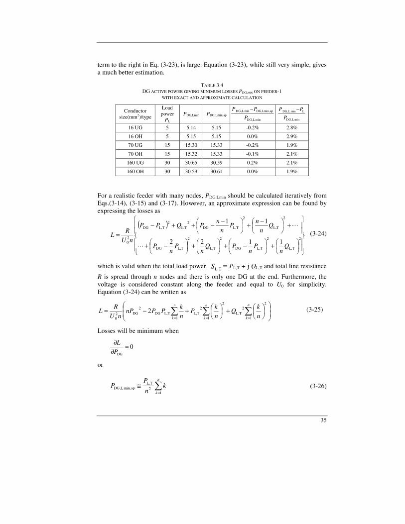
Table 3.4 shows PDG,Lmin on feeder-1 with exact and approximate calculations, for different conductors used and 0.8 (lagging) pfL. The table shows that for Feeder-1, with one load and one DG at the end of the feeder, PDG,Lmin,ap is very close to PDG,Lmin (calculated iteratively from the LSM). The table also shows that, if PDG,Lmin is estimated equal to PL, the error can be as high as 3% in case of small cross-section of the feeder conductor, when the resistance is high and therefore the error, which is the
35
term to the right in Eq. (3-23), is large. Equation (3-23), while still very simple, gives a much better estimation.
TABLE 3.4
DG ACTIVE POWER GIVING MINIMUM LOSSES PDG,MIN ON FEEDER-1 WITH EXACT AND APPROXIMATE CALCULATION
Conductor size(mm2)/type
Load power
PL (kW)
PDG,Lmin PDG,Lmin,ap minL,DG
apLmin,DG,minL,DG
P
PP −
minL,DG
LminL,DG
P
PP −
16 UG 5 5.14 5.15 -0.2% 2.8%
16 OH 5 5.15 5.15 0.0% 2.9%
70 UG 15 15.30 15.33 -0.2% 1.9%
70 OH 15 15.32 15.33 -0.1% 2.1%
160 UG 30 30.65 30.59 0.2% 2.1%
160 OH 30 30.59 30.61 0.0% 1.9%
For a realistic feeder with many nodes, PDG,Lmin should be calculated iteratively from Eqs.(3-14), (3-15) and (3-17). However, an approximate expression can be found by expressing the losses as
( )
+
−+
+
−+
+
−+
−−++−=
2
TL,
2
TL,DG
2
TL,
2
TL,DG
2
TL,
2
TL,DG2
TL,2
TL,DG
20 1122
11
Qn
Pn
PQn
Pn
P
Qn
nP
nn
PQPP
nUR
L
(3-24)
which is valid when the total load power TL,S = PL,T + j QL,T and total line resistance
R is spread through n nodes and there is only one DG at the end. Furthermore, the voltage is considered constant along the feeder and equal to U0 for simplicity. Equation (3-24) can be written as
+
+−= ===
n
k
n
k
n
k nk
Qnk
Pnk
PPnPnU
RL
1
22
TL,1
22
TL,1
TL,DG2
DG20
2 (3-25)
Losses will be minimum when
0DG
=∂∂PL
or
=
≅n
k
kn
PP
12TL,
apmin,L,DG (3-26)
Chapter 3: Voltage Control on LV Feeder with DG
36
By using the identity
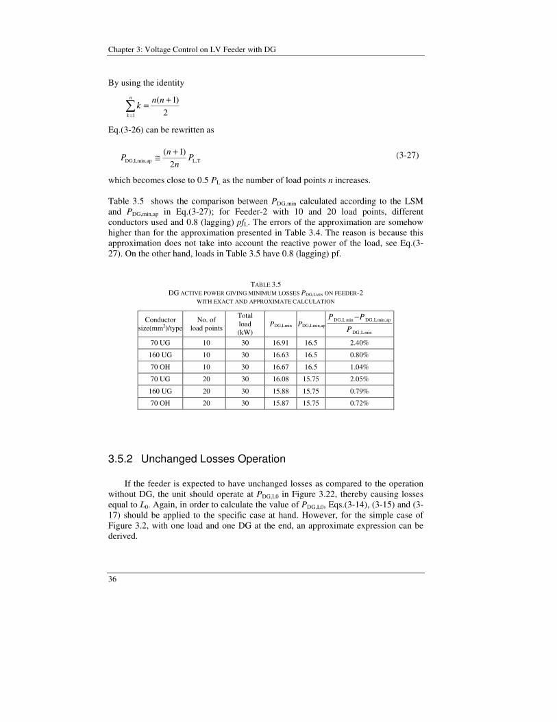
2
)1(
1
+==
nnk
n
k
Eq.(3-26) can be rewritten as
TL,apLmin,DG, 2)1(
Pn
nP
+≅ (3-27)
which becomes close to 0.5 PL as the number of load points n increases. Table 3.5 shows the comparison between PDG,min calculated according to the LSM and PDG,min,ap in Eq.(3-27); for Feeder-2 with 10 and 20 load points, different conductors used and 0.8 (lagging) pfL. The errors of the approximation are somehow higher than for the approximation presented in Table 3.4. The reason is because this approximation does not take into account the reactive power of the load, see Eq.(3-27). On the other hand, loads in Table 3.5 have 0.8 (lagging) pf.
TABLE 3.5 DG ACTIVE POWER GIVING MINIMUM LOSSES PDG,LMIN ON FEEDER-2
WITH EXACT AND APPROXIMATE CALCULATION
Conductor size(mm2)/type
No. of load points
Total load (kW)
PDG,Lmin PDG,Lmin,apminL,DG
apmin,L,DGminL,DG
P
PP −
70 UG 10 30 16.91 16.5 2.40%
160 UG 10 30 16.63 16.5 0.80%
70 OH 10 30 16.67 16.5 1.04%
70 UG 20 30 16.08 15.75 2.05%
160 UG 20 30 15.88 15.75 0.79%
70 OH 20 30 15.87 15.75 0.72%
3.5.2 Unchanged Losses Operation If the feeder is expected to have unchanged losses as compared to the operation without DG, the unit should operate at PDG,L0 in Figure 3.22, thereby causing losses equal to L0. Again, in order to calculate the value of PDG,L0, Eqs.(3-14), (3-15) and (3-17) should be applied to the specific case at hand. However, for the simple case of Figure 3.2, with one load and one DG at the end, an approximate expression can be derived.
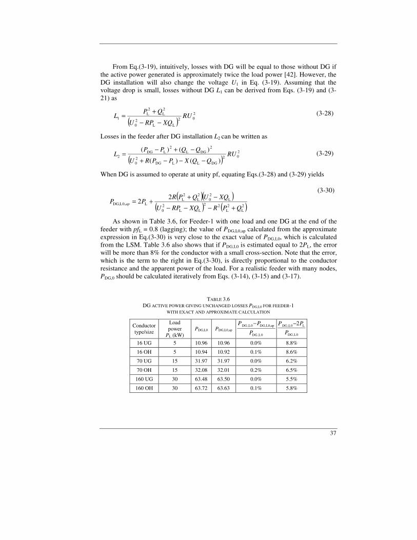
37
From Eq.(3-19), intuitively, losses with DG will be equal to those without DG if the active power generated is approximately twice the load power [42]. However, the DG installation will also change the voltage U1 in Eq. (3-19). Assuming that the voltage drop is small, losses without DG L1 can be derived from Eqs. (3-19) and (3-21) as
( )
202
LL20
2L
2L
1 RUXQRPU
QPL
−−
+= (3-28)
Losses in the feeder after DG installation L2 can be written as
( )
202
DGLLDG20
2DGL
2LDG
2)()(
)()(RU
QQXPPRU
QQPPL
−−−+
−+−= (3-29)
When DG is assumed to operate at unity pf, equating Eqs.(3-28) and (3-29) yields
( )( )
( ) ( )2L
2L
22
LL20
L20
2L
2L
L,0LDG,
22
QPRXQRPU
XQUQPRPP ap
+−−−−++=
(3-30)
As shown in Table 3.6, for Feeder-1 with one load and one DG at the end of the feeder with pfL = 0.8 (lagging); the value of PDG,L0,ap calculated from the approximate expression in Eq.(3-30) is very close to the exact value of PDG,L0, which is calculated from the LSM. Table 3.6 also shows that if PDG,L0 is estimated equal to 2PL, the error will be more than 8% for the conductor with a small cross-section. Note that the error, which is the term to the right in Eq.(3-30), is directly proportional to the conductor resistance and the apparent power of the load. For a realistic feeder with many nodes, PDG,0 should be calculated iteratively from Eqs. (3-14), (3-15) and (3-17).
TABLE 3.6 DG ACTIVE POWER GIVING UNCHANGED LOSSES PDG,L0 FOR FEEDER-1
WITH EXACT AND APPROXIMATE CALCULATION
Conductor type/size
Load power
PL (kW) PDG,L0 PDG,L0,ap
0L,DG
apL0,DG,0L,DG
P
PP −
0L,DG
L0L,DG 2
P
PP −
16 UG 5 10.96 10.96 0.0% 8.8%
16 OH 5 10.94 10.92 0.1% 8.6%
70 UG 15 31.97 31.97 0.0% 6.2%
70 OH 15 32.08 32.01 0.2% 6.5%
160 UG 30 63.48 63.50 0.0% 5.5%
160 OH 30 63.72 63.63 0.1% 5.8%
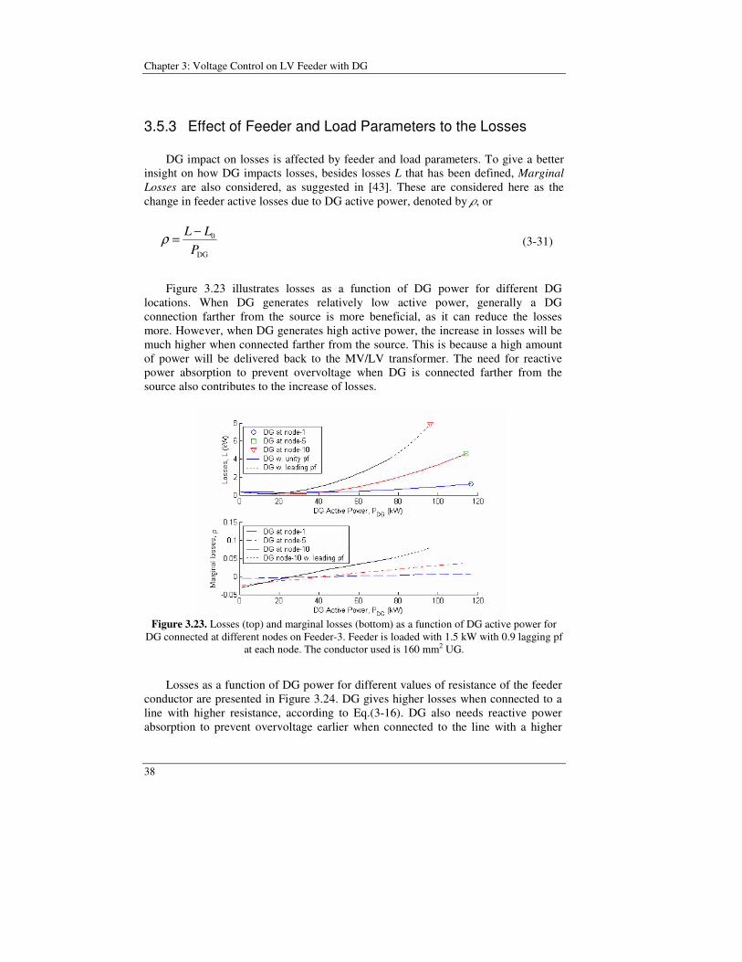
Chapter 3: Voltage Control on LV Feeder with DG
38
3.5.3 Effect of Feeder and Load Parameters to the Losses DG impact on losses is affected by feeder and load parameters. To give a better insight on how DG impacts losses, besides losses L that has been defined, Marginal Losses are also considered, as suggested in [43]. These are considered here as the change in feeder active losses due to DG active power, denoted by , or
DG
0
PLL −=ρ (3-31)
Figure 3.23 illustrates losses as a function of DG power for different DG locations. When DG generates relatively low active power, generally a DG connection farther from the source is more beneficial, as it can reduce the losses more. However, when DG generates high active power, the increase in losses will be much higher when connected farther from the source. This is because a high amount of power will be delivered back to the MV/LV transformer. The need for reactive power absorption to prevent overvoltage when DG is connected farther from the source also contributes to the increase of losses.
Figure 3.23. Losses (top) and marginal losses (bottom) as a function of DG active power for
DG connected at different nodes on Feeder-3. Feeder is loaded with 1.5 kW with 0.9 lagging pf at each node. The conductor used is 160 mm2 UG.
Losses as a function of DG power for different values of resistance of the feeder conductor are presented in Figure 3.24. DG gives higher losses when connected to a line with higher resistance, according to Eq.(3-16). DG also needs reactive power absorption to prevent overvoltage earlier when connected to the line with a higher
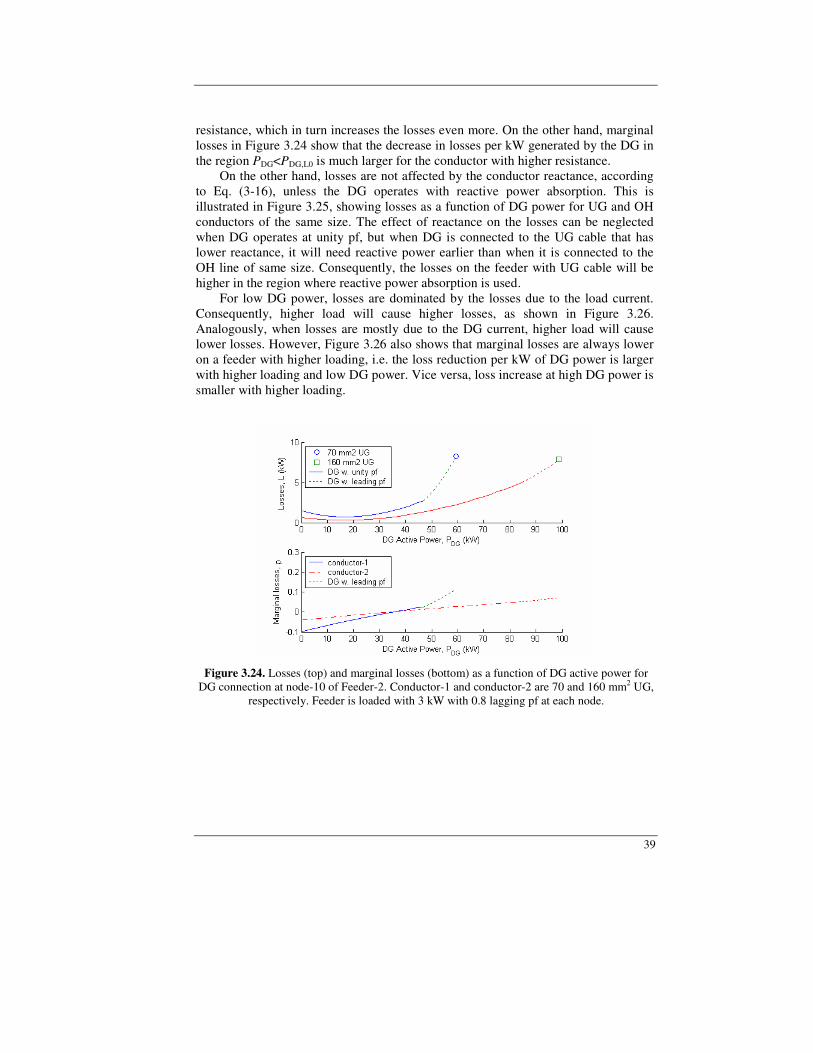
39
resistance, which in turn increases the losses even more. On the other hand, marginal losses in Figure 3.24 show that the decrease in losses per kW generated by the DG in the region PDG<PDG,L0 is much larger for the conductor with higher resistance. On the other hand, losses are not affected by the conductor reactance, according to Eq. (3-16), unless the DG operates with reactive power absorption. This is illustrated in Figure 3.25, showing losses as a function of DG power for UG and OH conductors of the same size. The effect of reactance on the losses can be neglected when DG operates at unity pf, but when DG is connected to the UG cable that has lower reactance, it will need reactive power earlier than when it is connected to the OH line of same size. Consequently, the losses on the feeder with UG cable will be higher in the region where reactive power absorption is used. For low DG power, losses are dominated by the losses due to the load current. Consequently, higher load will cause higher losses, as shown in Figure 3.26. Analogously, when losses are mostly due to the DG current, higher load will cause lower losses. However, Figure 3.26 also shows that marginal losses are always lower on a feeder with higher loading, i.e. the loss reduction per kW of DG power is larger with higher loading and low DG power. Vice versa, loss increase at high DG power is smaller with higher loading.
Figure 3.24. Losses (top) and marginal losses (bottom) as a function of DG active power for DG connection at node-10 of Feeder-2. Conductor-1 and conductor-2 are 70 and 160 mm2 UG,
respectively. Feeder is loaded with 3 kW with 0.8 lagging pf at each node.
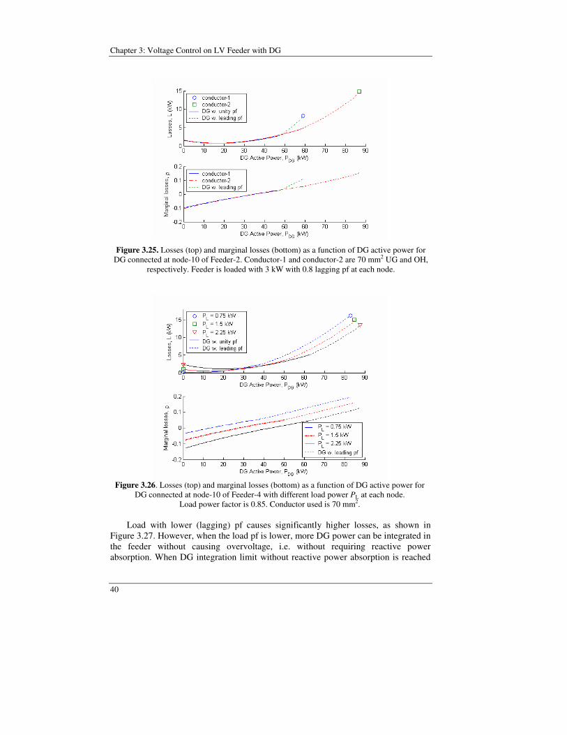
Chapter 3: Voltage Control on LV Feeder with DG
40
Figure 3.25. Losses (top) and marginal losses (bottom) as a function of DG active power for
DG connected at node-10 of Feeder-2. Conductor-1 and conductor-2 are 70 mm2 UG and OH, respectively. Feeder is loaded with 3 kW with 0.8 lagging pf at each node.
Figure 3.26. Losses (top) and marginal losses (bottom) as a function of DG active power for
DG connected at node-10 of Feeder-4 with different load power PL at each node. Load power factor is 0.85. Conductor used is 70 mm2.
Load with lower (lagging) pf causes significantly higher losses, as shown in Figure 3.27. However, when the load pf is lower, more DG power can be integrated in the feeder without causing overvoltage, i.e. without requiring reactive power absorption. When DG integration limit without reactive power absorption is reached

41
for a given load pf, e.g. 0.7 in Figure 3.27, losses are in fact comparable with those due to load with better (higher) pf, e.g. 0.85 in Figure 3.27. This is because lower losses due to the load current are compensated by higher losses due to the reactive current of the DG, requiring reactive power absorption.
Figure 3.27 Losses (top) and marginal losses (bottom) as a function of DG active power for
DG connected at node-10 of Feeder-2 in Figure 3.5 with different load power factor pfL. Load power is 4 kW at each node. Conductor used is 70 mm2 OH.
Chapter 3: Voltage Control on LV Feeder with DG
42
3.6 Conclusions In this chapter, voltage control in a LV feeder with DG has been investigated. It is shown that the well-known linear approximation for voltage calculation may lead to gross underestimation of the maximum voltage variation along the feeder. The loss summation model is instead shown to yield accurate results. Controlled reactive power absorption by the DG can significantly increase the maximum allowed DG active power with respect to feeder voltage limitation. However, when a certain amount of reactive power absorption is reached, which corresponds to the feeder being loaded at its ampacity, more reactive power will decrease the maximum allowed active power. The effectiveness of reactive power absorption for overvoltage mitigation and maximization of DG integration limit has been shown to depend on DG location, feeder and load parameters. The reactive power absorption for overvoltage mitigation will be more effective if the feeder is an overhead line rather than an underground cable. It will also be more effective when the conductor has a higher cross section. Reactive power absorption to maximize the DG integration limit will increase feeder losses and therefore should only be used when necessary. If DG is not designed to generate reactive power, the DG should be operated at unity power factor until Umax is reached. If more power has to be generated, the DG should be operated at voltage control mode by keeping the terminal voltage equal to Umax with reactive power absorption, until the amount of required power is fulfilled or the amount of tolerable losses is reached, as long as the feeder current is kept below the conductor ampacity. DG impact on losses is affected by DG location, feeder and load parameters. DG is most effective for loss reduction when the feeder has a high resistance, is highly loaded and the power factor of the load is low. Impact of feeder reactance is negligible unless the DG unit operates in voltage control mode.

Chapter 4
Voltage Control and Losses on LV
Feeder with Stochastic DG Output and
Load Power
This chapter analyzes voltage control and losses in a LV Feeder with photovoltaic (PV) generation by taking into account the fact that PV and load power stochastically vary. A probabilistic approach to the design of PV systems is treated. Monte Carlo simulation is used to predict the variation of solar radiation intensity and load, and LSM is used to solve the power flow. The method is tested on two study cases, and the results are compared with those from a deterministic approach based on commonly used scenarios. The probabilistic approach is shown necessary to obtain the optimum PV rating based on technical constraints and different objectives, including a reasonable risk.
4.1 Introduction Voltage control and losses with DG presented in Chapter 3 are based on a deterministic approach, i.e. both load and DG are assumed constant and known. Furthermore, the DG integration limit is defined based on minimum load – maximum generation scenario. Indeed, this scenario is commonly used by distribution network operators (DNOs) to define the DG integration limit. Some DNOs even assume no load – maximum generation as the worst case scenario [31]. However, in reality, the DG power output can vary stochastically, especially when the energy source is renewable, and also the load is not known with certainty, particularly in residential areas at LV level. For a stochastically variable sources DG, using the minimum load – maximum DG scenario to define DG integration limit will result in underestimation of the integration limit, as both minimum load and maximum generation may not occur at the same time.
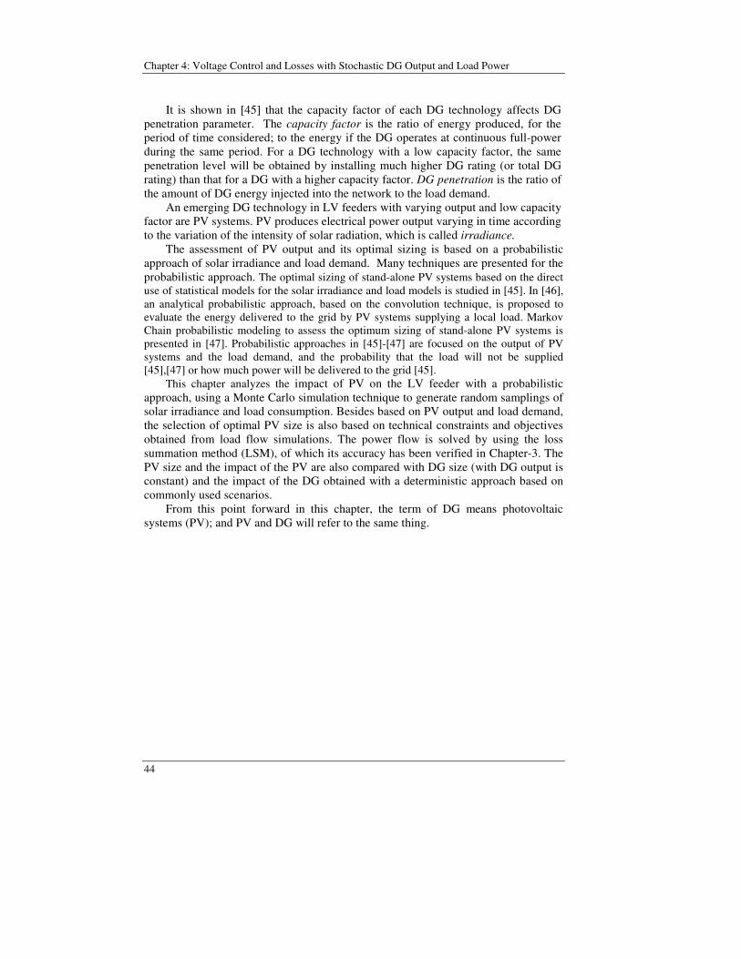
Chapter 4: Voltage Control and Losses with Stochastic DG Output and Load Power
44
It is shown in [45] that the capacity factor of each DG technology affects DG penetration parameter. The capacity factor is the ratio of energy produced, for the period of time considered; to the energy if the DG operates at continuous full-power during the same period. For a DG technology with a low capacity factor, the same penetration level will be obtained by installing much higher DG rating (or total DG rating) than that for a DG with a higher capacity factor. DG penetration is the ratio of the amount of DG energy injected into the network to the load demand. An emerging DG technology in LV feeders with varying output and low capacity factor are PV systems. PV produces electrical power output varying in time according to the variation of the intensity of solar radiation, which is called irradiance. The assessment of PV output and its optimal sizing is based on a probabilistic approach of solar irradiance and load demand. Many techniques are presented for the probabilistic approach. The optimal sizing of stand-alone PV systems based on the direct use of statistical models for the solar irradiance and load models is studied in [45]. In [46], an analytical probabilistic approach, based on the convolution technique, is proposed to evaluate the energy delivered to the grid by PV systems supplying a local load. Markov Chain probabilistic modeling to assess the optimum sizing of stand-alone PV systems is presented in [47]. Probabilistic approaches in [45]-[47] are focused on the output of PV systems and the load demand, and the probability that the load will not be supplied [45],[47] or how much power will be delivered to the grid [45]. This chapter analyzes the impact of PV on the LV feeder with a probabilistic approach, using a Monte Carlo simulation technique to generate random samplings of solar irradiance and load consumption. Besides based on PV output and load demand, the selection of optimal PV size is also based on technical constraints and objectives obtained from load flow simulations. The power flow is solved by using the loss summation method (LSM), of which its accuracy has been verified in Chapter-3. The PV size and the impact of the PV are also compared with DG size (with DG output is constant) and the impact of the DG obtained with a deterministic approach based on commonly used scenarios. From this point forward in this chapter, the term of DG means photovoltaic systems (PV); and PV and DG will refer to the same thing.
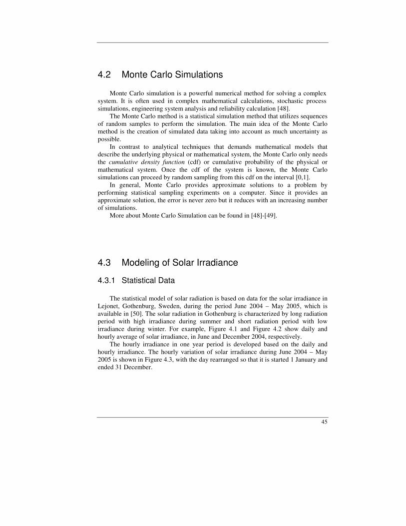
45
4.2 Monte Carlo Simulations
Monte Carlo simulation is a powerful numerical method for solving a complex system. It is often used in complex mathematical calculations, stochastic process simulations, engineering system analysis and reliability calculation [48].
The Monte Carlo method is a statistical simulation method that utilizes sequences of random samples to perform the simulation. The main idea of the Monte Carlo method is the creation of simulated data taking into account as much uncertainty as possible.
In contrast to analytical techniques that demands mathematical models that describe the underlying physical or mathematical system, the Monte Carlo only needs the cumulative density function (cdf) or cumulative probability of the physical or mathematical system. Once the cdf of the system is known, the Monte Carlo simulations can proceed by random sampling from this cdf on the interval [0,1].
In general, Monte Carlo provides approximate solutions to a problem by performing statistical sampling experiments on a computer. Since it provides an approximate solution, the error is never zero but it reduces with an increasing number of simulations.
More about Monte Carlo Simulation can be found in [48]-[49].
4.3 Modeling of Solar Irradiance
4.3.1 Statistical Data
The statistical model of solar radiation is based on data for the solar irradiance in Lejonet, Gothenburg, Sweden, during the period June 2004 – May 2005, which is available in [50]. The solar radiation in Gothenburg is characterized by long radiation period with high irradiance during summer and short radiation period with low irradiance during winter. For example, Figure 4.1 and Figure 4.2 show daily and hourly average of solar irradiance, in June and December 2004, respectively.
The hourly irradiance in one year period is developed based on the daily and hourly irradiance. The hourly variation of solar irradiance during June 2004 – May 2005 is shown in Figure 4.3, with the day rearranged so that it is started 1 January and ended 31 December.
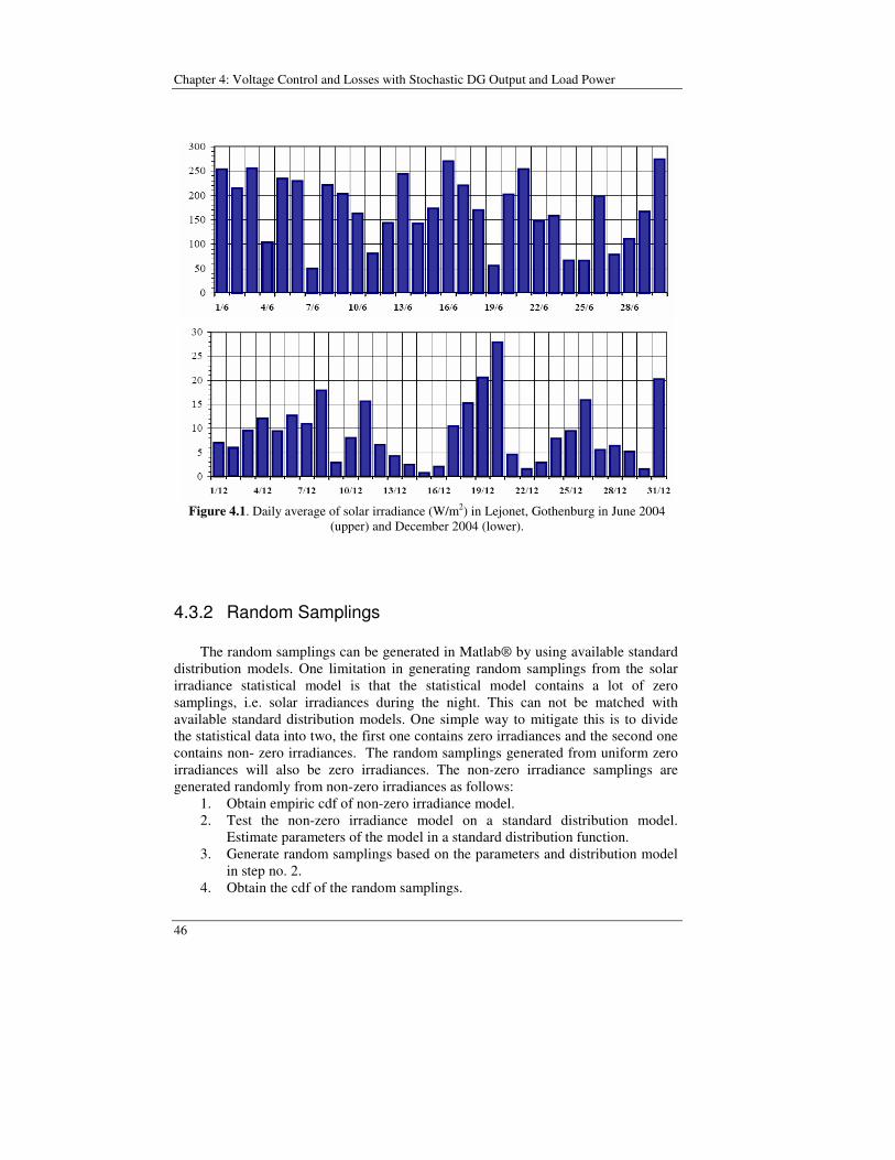
Chapter 4: Voltage Control and Losses with Stochastic DG Output and Load Power
46
Figure 4.1. Daily average of solar irradiance (W/m2) in Lejonet, Gothenburg in June 2004
(upper) and December 2004 (lower).
4.3.2 Random Samplings The random samplings can be generated in Matlab® by using available standard distribution models. One limitation in generating random samplings from the solar irradiance statistical model is that the statistical model contains a lot of zero samplings, i.e. solar irradiances during the night. This can not be matched with available standard distribution models. One simple way to mitigate this is to divide the statistical data into two, the first one contains zero irradiances and the second one contains non- zero irradiances. The random samplings generated from uniform zero irradiances will also be zero irradiances. The non-zero irradiance samplings are generated randomly from non-zero irradiances as follows:
1. Obtain empiric cdf of non-zero irradiance model. 2. Test the non-zero irradiance model on a standard distribution model.
Estimate parameters of the model in a standard distribution function. 3. Generate random samplings based on the parameters and distribution model
in step no. 2. 4. Obtain the cdf of the random samplings.
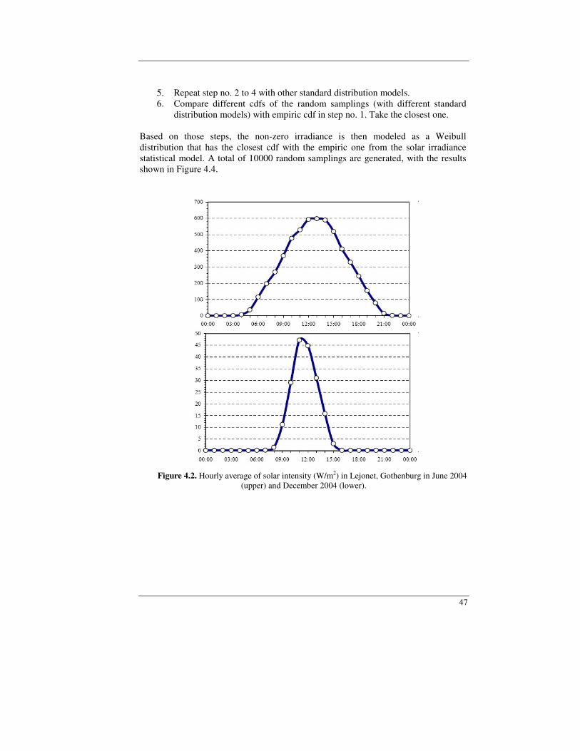
47
5. Repeat step no. 2 to 4 with other standard distribution models. 6. Compare different cdfs of the random samplings (with different standard
distribution models) with empiric cdf in step no. 1. Take the closest one. Based on those steps, the non-zero irradiance is then modeled as a Weibull distribution that has the closest cdf with the empiric one from the solar irradiance statistical model. A total of 10000 random samplings are generated, with the results shown in Figure 4.4.
Figure 4.2. Hourly average of solar intensity (W/m2) in Lejonet, Gothenburg in June 2004
(upper) and December 2004 (lower).
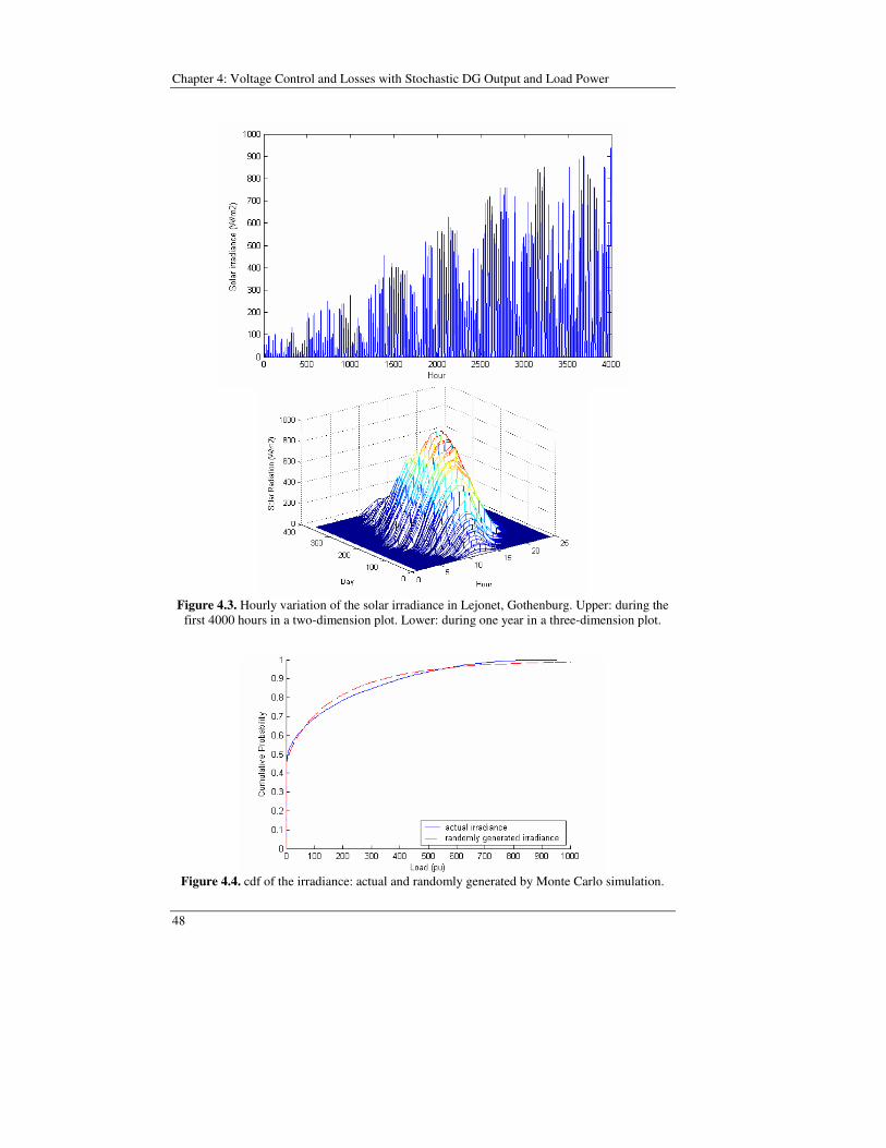
Chapter 4: Voltage Control and Losses with Stochastic DG Output and Load Power
48
Figure 4.3. Hourly variation of the solar irradiance in Lejonet, Gothenburg. Upper: during the
first 4000 hours in a two-dimension plot. Lower: during one year in a three-dimension plot.
Figure 4.4. cdf of the irradiance: actual and randomly generated by Monte Carlo simulation.
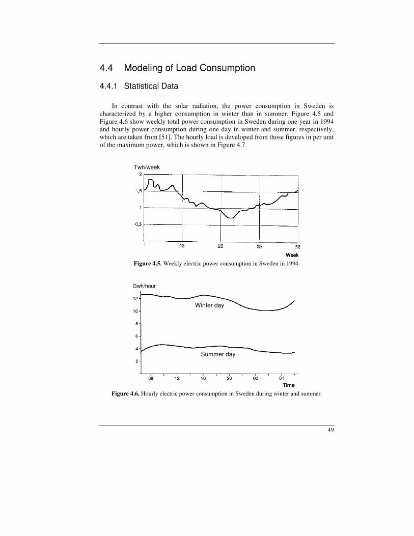
49
4.4 Modeling of Load Consumption
4.4.1 Statistical Data In contrast with the solar radiation, the power consumption in Sweden is characterized by a higher consumption in winter than in summer. Figure 4.5 and Figure 4.6 show weekly total power consumption in Sweden during one year in 1994 and hourly power consumption during one day in winter and summer, respectively, which are taken from [51]. The hourly load is developed from those figures in per unit of the maximum power, which is shown in Figure 4.7.
Week
Twh/week
WeekWeek
Twh/week
Figure 4.5. Weekly electric power consumption in Sweden in 1994.
Winter day
Summer day
Time
Gwh/hour
Winter day
Summer day
Time
Winter day
Summer day
Winter day
Summer day
Time
Gwh/hour
Figure 4.6. Hourly electric power consumption in Sweden during winter and summer.
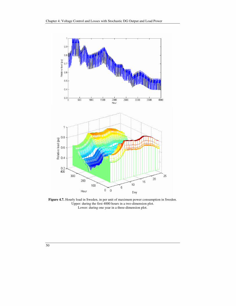
Chapter 4: Voltage Control and Losses with Stochastic DG Output and Load Power
50
Figure 4.7. Hourly load in Sweden, in per unit of maximum power consumption in Sweden.
Upper: during the first 4000 hours in a two-dimension plot. Lower: during one year in a three-dimension plot.
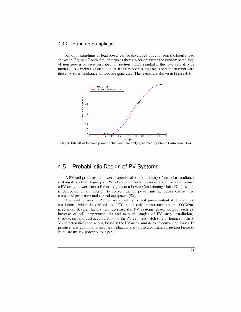
51
4.4.2 Random Samplings Random samplings of load power can be developed directly from the hourly load shown in Figure 4.7 with similar steps as they are for obtaining the random samplings of non-zero irradiance described in Section 4.3.2. Similarly, the load can also be modeled as a Weibull distribution. A 10000 random samplings, the same number with those for solar irradiance, of load are generated. The results are shown in Figure 4.8.
Figure 4.8. cdf of the load power: actual and randomly generated by Monte Carlo simulation.
4.5 Probabilistic Design of PV Systems A PV cell produces dc power proportional to the intensity of the solar irradiance
striking its surface. A group of PV cells are connected in series and/or parallel to form a PV array. Power from a PV array goes to a Power Conditioning Unit (PCU), which is composed of an inverter (to convert the dc power into ac power output) and associated protection and control equipment [52].
The rated power of a PV cell is defined by its peak power output at standard test conditions, which is defined as 250C solar cell temperature under 1000W/m2 irradiance. Several factors will decrease the PV systems power output, such as: increase of cell temperature, tilt and azimuth (angles of PV array installation), shadow, dirt and dust accumulation on the PV cell, mismatch (the difference in the I-V characteristics) and wiring losses in the PV array, and dc to ac conversion losses. In practice, it is common to assume no shadow and to use a constant correction factor to calculate the PV power output [52].

Chapter 4: Voltage Control and Losses with Stochastic DG Output and Load Power
52
As explained in Chapter 2, PV is a capital-intensive technology with very low operating costs. Thus, once a PV is installed, it is really important to maximize the power that the PV system can generate based on the available solar radiation.
With the correction factor assumed constant, the ac power output of PV system is assumed to be linearly proportional to the solar irradiance, with the power equal to the PV rating, when the solar radiation is 1000 W/m2, or higher, according to the standard test conditions. The number and size of PV cells, and tilt and azimuth of PV array installation to obtain the PV system with specified rating is not discussed in this thesis. Further, PV is assumed to be without energy storage. Two different cases are treated. The first case assumes that the PV installation is owned by a generation company and concentrated at one node in a PV farm, i.e. to allow deferring the upgrade of a MV distribution line due to high load growth. The objective in this case is the maximization of the power produced by the PV installation, taking into account the effect on feeder losses. The second case assumes that the PV is owned by individual customers and distributed along the feeder, representing e.g. PV installation on house roof. The objective function in this case is minimization of active power exchanged with the grid PL-PDG. Both cases are subjected to the following constraints:
1. Ui < Umax, nodes 2. PDG 3. 0 < PDG < PDG,rat
where PDG is the PV power output in kW. PDG,rat is the PV rating in kW. U is the voltage, and Umax is the maximum allowed voltage. is the solar irradiance in W/m2.
The proposed method is tested on feeder-4 shown in Figure 3.5 in Chapter 3, with the following additional quantities: • Voltage limit: Umax = 1.06 pu and Umin = 0.9 pu as applied in Chapter 3. • Conductor: 70 mm2 overhead (O/H) line, as specified in Table 3.1 in Chapter 3. • Load: constant power, uniformly distributed at each node, with PL,max = 2.510. This
load will represent 1.0 pu load in the probabilistic model. • In the first case study, the PV farm is connected to node-7, whereas in the second
case study, the PVs are connected at every node.

53
4.5.1 Case Study 1: PV Farm The flow chart of PV size selection on case study 1 presented in Figure 4.9 can be explained as follows:
1. The simulation is started by generating random samples of solar irradiance (in W/m2) and random samples of load power PL,pu (in per unit of maximum load).
2. Find maximum load of the feeder PL,max from conductor thermal capacity. 3. Select PV rating PDG,rat. 4. Calculate load power in kW PL. 5. Calculate PV power PDG, which is assumed to be linearly proportional to the
irradiance. 6. Calculate voltage at PV connection point UDG, feeder current I and feeder
losses L for PV operation at unity power factor. LSM described in Chapter-3 is used to solve this load flow calculation.
7. If voltage at PV connection point UDG is higher than maximum allowed voltage Umax, repeat step no 6 by operating the PV at leading power factor.
8. If steps no. 4 to 7 have been repeated for all random samplings of and PL,pu; average PV power PDG,ave and average losses Lave can be calculated.
9. If the test will be continued to different rating of PV, back to step no. 3. The cdf of voltage when a PV installation of different ratings is connected at node-7, shown in Figure 4.10, indicates that PV can be operated at unity power factor without reaching Umax as long as the rating of the PV is below 90 kW. For a higher rating there is a certain probability that Umax is reached and PV needs to be operated at leading power factor to deliver the corresponding active power. On the other hand, calculating the DG rating deterministically based on minimum load – maximum generation scenario yields a maximum rating for operation at unity power factor of less than 50 kW, as shown in Figure 4.11. Similar conclusions are valid when DG is operated at a leading power factor, after Umax is reached, i.e. when the active power is limited by the conductor ampacity. The cdf of feeder current when a PV installation of different ratings is connected at node-7, shown in Figure 4.12, indicates that the DG integration limit is around 95 kW. With a deterministic approach the corresponding limit based on a minimum load – maximum generation scenario is around 85 kW, see Figure 4.11.

Chapter 4: Voltage Control and Losses with Stochastic DG Output and Load Power
54
i = 1
Select PDG,rat(i)
j = 0
j = j+1
j > 10000 ?
)(000,1
)(),( ratDG,DG iP
jijP
β=
maxL,puL,L )()( PjPjP ⋅=
Randomly generatePL,pu(1:10000) (1:10000)
QDG(j,i) = 0
Calculate UDG(j,i), I(j,i), L(j,i)
k = 0
k = k+1
QDG(j,i) = - PDG(j,i) tan(cos-1(1-k/100))
Try anotherPDG,rat ?
Finish
yes
no
yes
10000
),()(
10000
),()(
10000
1
10000
1DG
aveDG,
=
=
=
=
jave
j
ijLiL
ijPiP
i = i+1
UDG(j,i) > Umax
no
no
yes
Calculate UDG(j,i), I(j,i), L(j,i)
Start
i = 1
Select PDG,rat(i)
j = 0
j = j+1
j > 10000 ?
)(000,1
)(),( ratDG,DG iP
jijP
β=
maxL,puL,L )()( PjPjP ⋅=
Randomly generatePL,pu(1:10000) (1:10000)
QDG(j,i) = 0
Calculate UDG(j,i), I(j,i), L(j,i)
k = 0
k = k+1
QDG(j,i) = - PDG(j,i) tan(cos-1(1-k/100))
Try anotherPDG,rat ?
FinishFinish
yes
no
yes
10000
),()(
10000
),()(
10000
1
10000
1DG
aveDG,
=
=
=
=
jave
j
ijLiL
ijPiP
10000
),()(
10000
),()(
10000
1
10000
1DG
aveDG,
=
=
=
=
jave
j
ijLiL
ijPiP
i = i+1
UDG(j,i) > Umax
no
no
yes
Calculate UDG(j,i), I(j,i), L(j,i)
Start
Figure 4.9. Flow chart to design PV on case study 1.
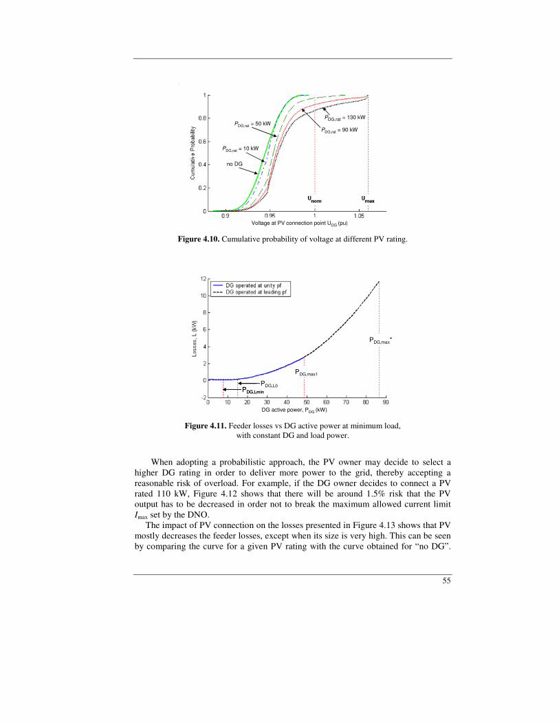
55
no DG
PDG,rat = 10 kW
PDG,rat = 50 kWPDG,rat = 90 kW
PDG,rat = 130 kW
Voltage at PV connection point UDG (pu)
no DG
PDG,rat = 10 kW
PDG,rat = 50 kWPDG,rat = 90 kW
PDG,rat = 130 kW
Voltage at PV connection point UDG (pu) Figure 4.10. Cumulative probability of voltage at different PV rating.
PDG,max1
PDG,max*
PDG,Lmin
PDG,L0
DG active power, PDG (kW)
PDG,max1
PDG,max*
PDG,Lmin
PDG,L0
PDG,max1
PDG,max*
PDG,Lmin
PDG,L0
DG active power, PDG (kW) Figure 4.11. Feeder losses vs DG active power at minimum load,
with constant DG and load power.
When adopting a probabilistic approach, the PV owner may decide to select a higher DG rating in order to deliver more power to the grid, thereby accepting a reasonable risk of overload. For example, if the DG owner decides to connect a PV rated 110 kW, Figure 4.12 shows that there will be around 1.5% risk that the PV output has to be decreased in order not to break the maximum allowed current limit Imax set by the DNO. The impact of PV connection on the losses presented in Figure 4.13 shows that PV mostly decreases the feeder losses, except when its size is very high. This can be seen by comparing the curve for a given PV rating with the curve obtained for “no DG”.
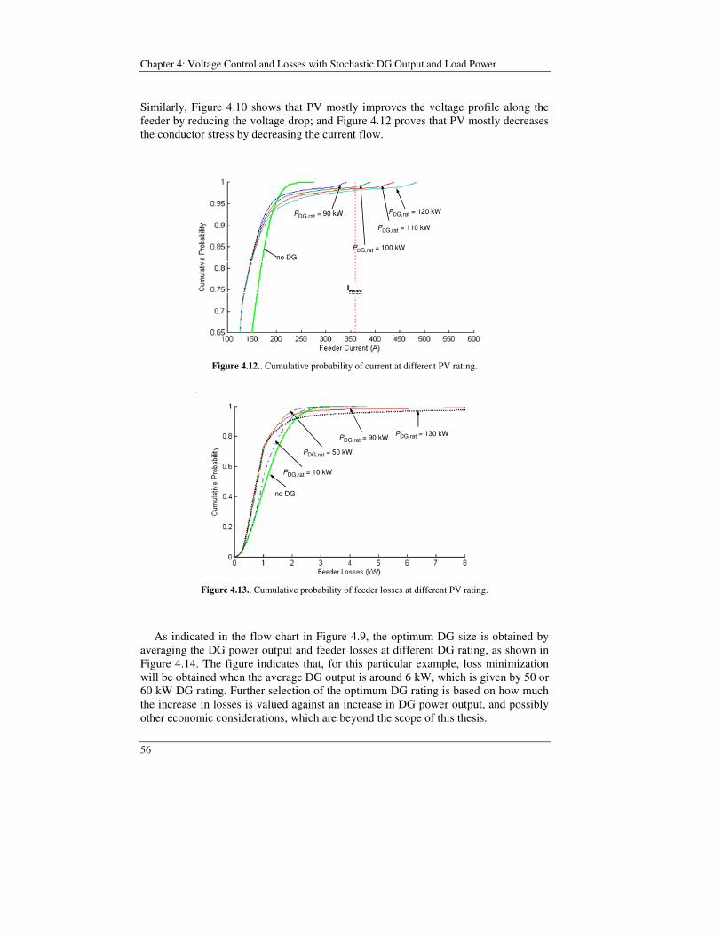
Chapter 4: Voltage Control and Losses with Stochastic DG Output and Load Power
56
Similarly, Figure 4.10 shows that PV mostly improves the voltage profile along the feeder by reducing the voltage drop; and Figure 4.12 proves that PV mostly decreases the conductor stress by decreasing the current flow.
no DG
PDG,rat = 90 kW PDG,rat = 120 kW
PDG,rat = 110 kW
PDG,rat = 100 kWno DG
PDG,rat = 90 kW PDG,rat = 120 kW
PDG,rat = 110 kW
PDG,rat = 100 kW
Figure 4.12.. Cumulative probability of current at different PV rating.
no DG
PDG,rat = 10 kW
PDG,rat = 50 kW
PDG,rat = 90 kW PDG,rat = 130 kW
no DG
PDG,rat = 10 kW
PDG,rat = 50 kW
PDG,rat = 90 kW PDG,rat = 130 kW
Figure 4.13.. Cumulative probability of feeder losses at different PV rating.
As indicated in the flow chart in Figure 4.9, the optimum DG size is obtained by averaging the DG power output and feeder losses at different DG rating, as shown in Figure 4.14. The figure indicates that, for this particular example, loss minimization will be obtained when the average DG output is around 6 kW, which is given by 50 or 60 kW DG rating. Further selection of the optimum DG rating is based on how much the increase in losses is valued against an increase in DG power output, and possibly other economic considerations, which are beyond the scope of this thesis.

57
PDG,rat = 10 kW
PDG,rat = 140 kW
PDG,rat = 110 kW
PDG,rat isincreased by 10 kW
PDG,rat = 10 kW
PDG,rat = 140 kW
PDG,rat = 110 kW
PDG,rat isincreased by 10 kW
Figure 4.14. Average losses as a function of average PV power output at different DG rating.
Finally, predicting the DG impact on losses with a deterministic approach leads to underestimating the capability of DG to decrease feeder losses. In the case presented, loss calculation with a deterministic approach based on minimum load scenario shown in Figure 4.11 indicates that DG will always increase the feeder losses, unless its size is less than 15 kW. This is contrast with Figure 4.14, which indicates that the PV will decrease the losses, except when the DG rating is more than 110 kW.
4.5.2 Case Study 2: Distributed PV The flow chart of PV size selection on study case-2 presented in Figure 4.15. In contrast with the previous case, load flow simulation is not necessary to be run, as the objective of the DG installation by customer is to minimize their power consumption from the grid, PL-PDG. Indeed, PL and PDG can be obtained directly from the generated random samplings.
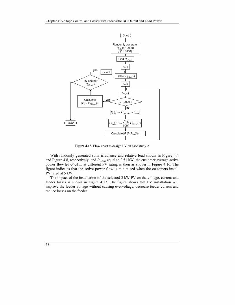
Chapter 4: Voltage Control and Losses with Stochastic DG Output and Load Power
58
Find PL,max
i = 1
Select PDG,rat(i)
j = 0
j = j+1
j > 10000 ?
)()(
),( ratDG,DG iPj
ijP1000β=
maxL,puL,L )()( PjPjP ⋅=
Calculate PL(j)-PDG(j,i)
yes
no
i = i+1
Try anotherPDG,rat ?
Finish
yes
CalculatePL – PDGave(i)
Randomly generatePL,pu(1:10000)(1:10000)
Start
Find PL,max
i = 1
Select PDG,rat(i)
j = 0
j = j+1
j > 10000 ?
)()(
),( ratDG,DG iPj
ijP1000β=
maxL,puL,L )()( PjPjP ⋅=
Calculate PL(j)-PDG(j,i)
yes
no
i = i+1
Try anotherPDG,rat ?
Finish
yes
CalculatePL – PDGave(i)
Randomly generatePL,pu(1:10000)(1:10000)
StartStart
Figure 4.15. Flow chart to design PV on case study 2. With randomly generated solar irradiance and relative load shown in Figure 4.4 and Figure 4.8, respectively; and PL,max equal to 2.51 kW, the customer average active power flow PL-PDG,ave at different PV rating is then as shown in Figure 4.16. The figure indicates that the active power flow is minimized when the customers install PV rated at 5 kW. The impact of the installation of the selected 5 kW PV on the voltage, current and feeder losses is shown in Figure 4.17. The figure shows that PV installation will improve the feeder voltage without causing overvoltage, decrease feeder current and reduce losses on the feeder.

59
PL –
PD
G a
ve (k
W)
PL –
PD
G a
ve (k
W)
Figure 4.16. Average customer active power flow PL-PDGave at different DG rating.
Figure 4.17. Voltage (top), current (middle) and losses (bottom)
before and after PV installation.
Chapter 4: Voltage Control and Losses with Stochastic DG Output and Load Power
60
4.6 Conclusions In this thesis, the use of probabilistic methods to the design of PV systems has been treated. The stochastic variability of both generation and load has been considered. A method for selection of the optimal size of a PV system, based on actual hourly solar radiation in Gothenburg, Sweden, and typical hourly load in Sweden has been presented. The same method can be used to evaluate the impact of PVof a given size on the distribution network. It has been demonstrated that, when the energy source is varying stochastically, limiting the DG integration based on minimum load – maximum generation scenario results in underestimation of the DG integration limit, since minimum load and maximum generation may not occur at the same time. When the DG is intended to deliver as much power as possible, this approach makes it possible to define an acceptable risk of overload that the DG owner may accept in order to install DG of higher rating, thereby being able to deliver more power to the network. Furthermore, it was demonstrated that the positive impact of PV-based DG on losses is also grossly underestimated when using a deterministic method. For completeness, the use of Monte Carlo simulation to investigate the PV size selection when the PV is owned by an individual customer interested in minimizing the active power drawn from the grid has also been examined. Finally, it should be remarked that, in the example shown, the PV will most probably improve the voltage profile and decrease the losses in the feeder.
Chapter 5
Voltage Control on Medium Voltage
Feeders with Distributed Generation
This chapter discusses different voltage control methods on MV feeders with the presence of DG. Voltage control by on-load tap changers (LTCs) and Line Drop Compensation (LDC) on MV Feeders is examined, and how these voltage regulations are affected by DG is analyzed. The voltage regulation constraints with LTC and LDC are reformulated for the case of DG connected along a feeder in a single- or multi-feeder system. Voltage control by using a line voltage regulator (VR), DG reactive power and feeder operation in a closed-loop are also discussed briefly. The DG integration limits with different voltage control methods are then compared.
5.1 Introduction Voltage control of MV distribution feeders can be achieved by using on-load tap changers and capacitor banks. The LTC keeps the voltage at the substation busbar constant. Normally, a LTC is also provided with line drop compensation (LDC) to keep the voltage constant at a remote load center (LC) [2],[53]-[55]. LTCs are widespread in distribution networks and are likely to remain in service for many years to come [55]. DG causes reduction or possibly reversal of real power flows, which may impart significant power factor changes detected by a HV/MV transformer. These changes may affect the effectiveness of the voltage regulation provided by LDC. Therefore, DG should be coordinated with LDC to ensure that the distribution network will not loose the function of proper voltage regulation. Proper coordination is also necessary in order to ensure that the DG integration will not be unnecessarily limited. The DG integration limit has been defined in Chapter 3, where the transformer constraint STX is referred to the rating of the upstream HV/MV transformer. The reduction or reversal of active power flow due to DG will increase the voltage along the feeder. DG coordination with switched capacitor banks is also required to ensure that the capacitors will not cause overvoltages [56].
Chapter 5: Voltage Control on MV Feeder with DG
62
Voltage controls in MV Feeders with the presence of DG have been presented in several papers. On a feeder with LTC regulation, the sending end voltage U0, at the substation busbar, is kept constant, and a DG connection will increase the voltage profile on the feeder, which may lead to overvoltage. Thus, the reduction of the LTC setting in a HV/MV substation will increase the DG integration limit, as presented in [57]. However, when the limiting point is the minimum allowed voltage Umin at the end of the feeder, the use of LDC may increase the DG integration limit. In [58], the maximum DG integration limit on multiple feeders with LDC is derived mathematically. The proposed calculation method is based on the relation of sending end voltage and DG power factor to the maximum DG integration limit. Voltage at all nodes of all feeders will be within permissible range and the LTC tap will not operate with the introduction of DG. The change in voltage profile can be minimized with this method. However, the integration limit obtained by preventing LTC from changing its position will be very marginal. More DG power can be introduced without violating the permissible voltage limits when the LTC tap position is allowed to change. In [31] and [59], the installation of a line voltage regulator (VR) is presented to solve unacceptable voltage variations. The installation of additional VR in a feeder with DG to prevent overvoltage, is similar to the installation of VR in a conventional feeder with only loads to prevent undervoltage. This method allows the connection of a larger amount of DG power to the feeder. However, VR installation means additional investment costs. Improvement of LDC performance is proposed in [60] by utilizing multiple LDCs (MLDCs) on multiple feeders with different loading. The performance of MLDCs is shown to be more accurate and flexible than that of the conventional LDC method, with the drawback that the tap changing operation of MLDC occurs more frequently than that of the conventional LDC. This method is based on system-wide coordination of voltages using remote control, communication and optimization. Besides the need of a communication link and the modification of the existing LDC control system, the voltage control of the distribution network is far more complicated when using this method [57], which may be considered undesirable by many DNOs nowadays. On a distribution system of several feeders fed by one HV/MV transformer, DG will deteriorate the voltage control when the DG is connected on a feeder which is lightly loaded, and at the same time the adjacent feeder – which is fed by the same transformer – is highly loaded. DG may cause overvoltage on the feeder where it is connected, whereas the highly loaded feeder may suffer undervoltage. Operating the distribution feeder in a meshed system will minimize the voltage unbalance among the feeders and increase the DG integration limit, as presented in [57] and [61]. One major concern with operating feeder in a meshed system is the increase in short circuit current [62] and protection of the distribution system. Protection of meshed distribution network with DG will be discussed in Chapter 7 of this thesis.
63
5.2 Voltage Control in Conventional MV Feeder with LTC/LDC
The objective of voltage control in conventional feeders, i.e., feeders with only loads and no DG connected, can be either to minimize feeder losses or to operate the feeder close to the nominal voltage. One means of voltage control is the LTC regulator, which is an autotransformer with automatically adjusted taps. Commonly, a LTC provides a regulation range from -10% to 10% using 32 steps [2],[53]-[54]. The LTC will keep the voltage constant at the local busbar, or at a LC, if provided with LDC. In practice, many LTCs are operated with the LDC feature disabled, which is much simpler. In this chapter, voltage regulation using both LTC with LDC disabled (called LTC regulation) and LTC with LDC activated (called LDC regulation) are analyzed. Another means of voltage control are capacitor banks, which inject reactive power into the feeder, thus decreasing the line current and losses and increasing the voltage. Capacitors can either be fixed or switched by capacitor control. Many capacitor controls can be used in conventional MV feeders, such as time control, voltage control, current control and VAR control [2].
5.2.1 Voltage Control with LTC Regulation The basic arrangement of voltage control with LTC regulation is shown in Figure 5.1. The LTC will keep the local busbar voltage, i.e. the sending end voltage U0, constant within the range
ULB < U0 < UUB (5-1)
where ULB = Uset – 0.5 bandwidth is the lower boundary voltage; UUB = Uset + 0.5 bandwidth is the upper boundary voltage; Uset is the setpoint voltage.
The voltage of a conventional MV feeder decreases towards the end. The LTC shall then be set to ensure that the voltage at the feeder end is higher than the minimum allowed voltage Umin, and the sending-end voltage is lower than the maximum allowed voltage Umax. Since the LTC keeps the sending-end voltage U0 constant, it is possible to operate the feeder with minimum losses at any load condition. No load or feeder parameters appear in Eq. (5-1), so LTC regulation will not be affected by changes in the pf or reversal of active/reactive power. With the sending-end voltage kept constant, multiple-feeders controlled by the same LTC can be treated
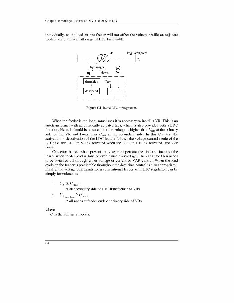
Chapter 5: Voltage Control on MV Feeder with DG
64
individually, as the load on one feeder will not affect the voltage profile on adjacent feeders, except in a small range of LTC bandwidth.
USET
deadband
timedelay
tapchanger
up down
+ -
Regulated point
U0
USET
deadband
timedelay
tapchanger
up down
+ -
Regulated point
U0
Figure 5.1. Basic LTC arrangement. When the feeder is too long, sometimes it is necessary to install a VR. This is an autotransformer with automatically adjusted taps, which is also provided with a LDC function. Here, it should be ensured that the voltage is higher than Umin at the primary side of the VR and lower than Umax at the secondary side. In this Chapter, the activation or deactivation of the LDC feature follows the voltage control mode of the LTC; i.e. the LDC in VR is activated when the LDC in LTC is activated, and vice versa. Capacitor banks, when present, may overcompensate the line and increase the losses when feeder load is low, or even cause overvoltage. The capacitor then needs to be switched off through either voltage or current or VAR control. When the load cycle on the feeder is predictable throughout the day, time control is also appropriate. Finally, the voltage constraints for a conventional feeder with LTC regulation can be simply formulated as
i. max0 UU ≤ ,
all secondary side of LTC transformer or VRs
ii. minloadmax i UU ≥ ,
all nodes at feeder-ends or primary side of VRs
where Ui is the voltage at node i.
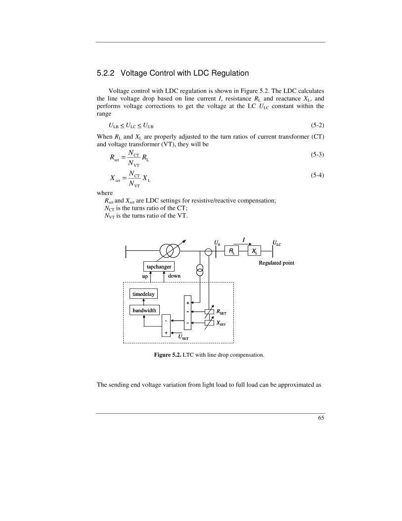
65
5.2.2 Voltage Control with LDC Regulation
Voltage control with LDC regulation is shown in Figure 5.2. The LDC calculates the line voltage drop based on line current I, resistance RL and reactance XL, and performs voltage corrections to get the voltage at the LC ULC constant within the range
ULB < ULC < UUB (5-2)
When RL and XL are properly adjusted to the turn ratios of current transformer (CT) and voltage transformer (VT), they will be
L
VT
CTset R
NN
R = (5-3)
L
VT
CTset X
NN
X = (5-4)
where Rset and Xset are LDC settings for resistive/reactive compensation; NCT is the turns ratio of the CT; NVT is the turns ratio of the VT.
RL XL
RSET
XSET-
+USET
bandwidth
timedelay
tapchanger
up down
Regulated point
ULC
+
-
-
U0I
RL XL
RSET
XSET-
+USET
bandwidth
timedelay
tapchanger
up down
Regulated point
ULC
+
-
-
+
-
-
U0I
Figure 5.2. LTC with line drop compensation. The sending end voltage variation from light load to full load can be approximated as

Chapter 5: Voltage Control on MV Feeder with DG
66
)sincos()sincos( LLLLLLFLLL0,FL0, φφφφ XRIXRIUU +−+=− (5-5)
where U0,FL and U0,LL are full load and light load sending-end voltage at substation MV bus, respectively; IFL and ILL are full load and light load line current; cos is pf at LTC location.
The LDC setpoint voltage can be derived from Eq.(5-5) as
LL
LLFL
LL,0FL,0LL,0set I
IIUU
UU−−
−= (5-6)
As the LDC boosts the voltage most during high load and least during light load, the feeder can be operated close to its nominal voltage at any load condition. However, minimization of losses at any load condition cannot be achieved. As LDC regulation employs load and feeder parameters, see Eqs.(5-5)-(5-6), changes in the pf or direction of active/reactive power will affect the performance of the regulator [2]. One case is when the X/R ratio of the setting is poorly adjusted [55]. For example, consider a feeder with a load at the LC regulated by LDC in Figure 5.3(a). LDC tries to keep the voltage at the load constant by adjusting the sending-end voltage as
)sincos( HVset,HVset,set0 φφ XRIUU ++= (5-7)
where Rset,HV and Xset,HV are Rset and Xset read on primary side of the CT and VT. With the sending-end voltage as in (5-7), the actual voltage at LC is then
)sincos( LL0LC φφ XRIUU +−= (5-8)
If Rset is properly adjusted, i.e. Rset= RL, the voltage error at the LC is
−=−
L
L
set
setLsetLC sin
RX
RX
IRUU φ (5-9)
The error increases with decreasing pf and increasing load, for instance as shown in Figure 5.3(b).
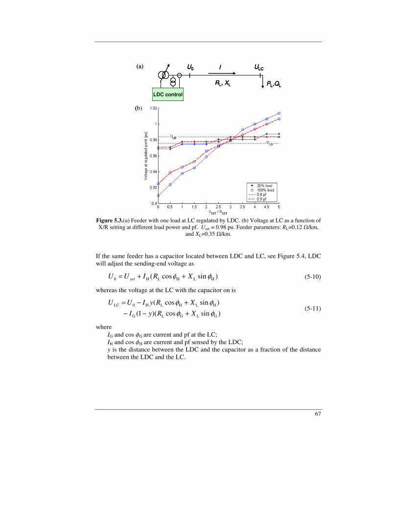
67
U0 ULC
PL,QL
I
RL, XL
LDC control
U0 ULC
PL,QL
I
RL, XL
LDC controlLDC control
(a) U0 ULC
PL,QL
I
RL, XL
LDC control
U0 ULC
PL,QL
I
RL, XL
LDC controlLDC control
(a)
(b)(b)
Figure 5.3.(a) Feeder with one load at LC regulated by LDC. (b) Voltage at LC as a function of X/R setting at different load power and pf. Uset = 0.98 pu. Feeder parameters: RL=0.12 /km,
and XL=0.35 /km. If the same feeder has a capacitor located between LDC and LC, see Figure 5.4, LDC will adjust the sending-end voltage as
)sincos( HLHLH0 φφ XRIUU set ++= (5-10)
whereas the voltage at the LC with the capacitor on is
)sincos)(1(
)sincos(
GLGLG
HLHLH0LC
φφφφ
XRyI
XRyIUU
+−−+−=
(5-11)
where IG and cos G are current and pf at the LC;
IH and cos H are current and pf sensed by the LDC; y is the distance between the LDC and the capacitor as a fraction of the distance between the LDC and the LC.
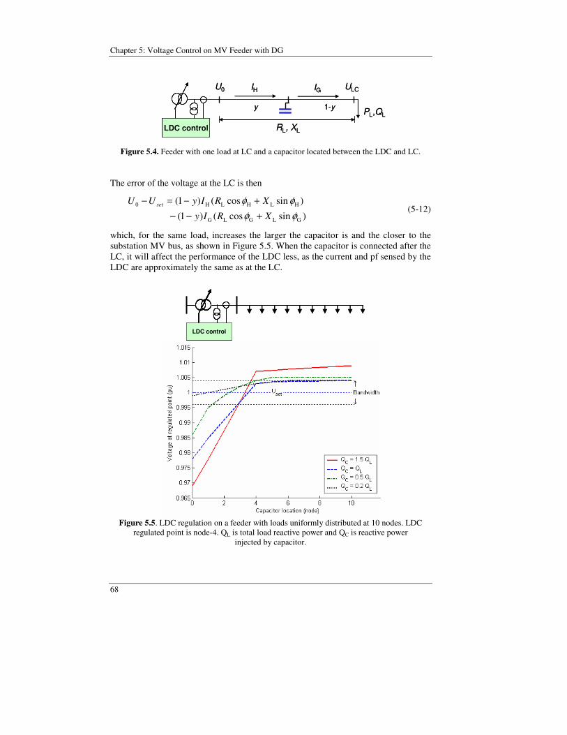
Chapter 5: Voltage Control on MV Feeder with DG
68
U0 ULC
PL,QL
IG
RL, XLLDC control
IH
y 1-y
U0 ULC
PL,QL
IG
RL, XLLDC controlLDC control
IH
y 1-y
Figure 5.4. Feeder with one load at LC and a capacitor located between the LDC and LC. The error of the voltage at the LC is then
)sincos()1(
)sincos()1(
GLGLG
HLHLH0
φφφφ
XRIy
XRIyUU set
+−−+−=−
(5-12)
which, for the same load, increases the larger the capacitor is and the closer to the substation MV bus, as shown in Figure 5.5. When the capacitor is connected after the LC, it will affect the performance of the LDC less, as the current and pf sensed by the LDC are approximately the same as at the LC.
LDC controlLDC controlLDC controlLDC controlLDC control
Figure 5.5. LDC regulation on a feeder with loads uniformly distributed at 10 nodes. LDC
regulated point is node-4. QL is total load reactive power and QC is reactive power injected by capacitor.
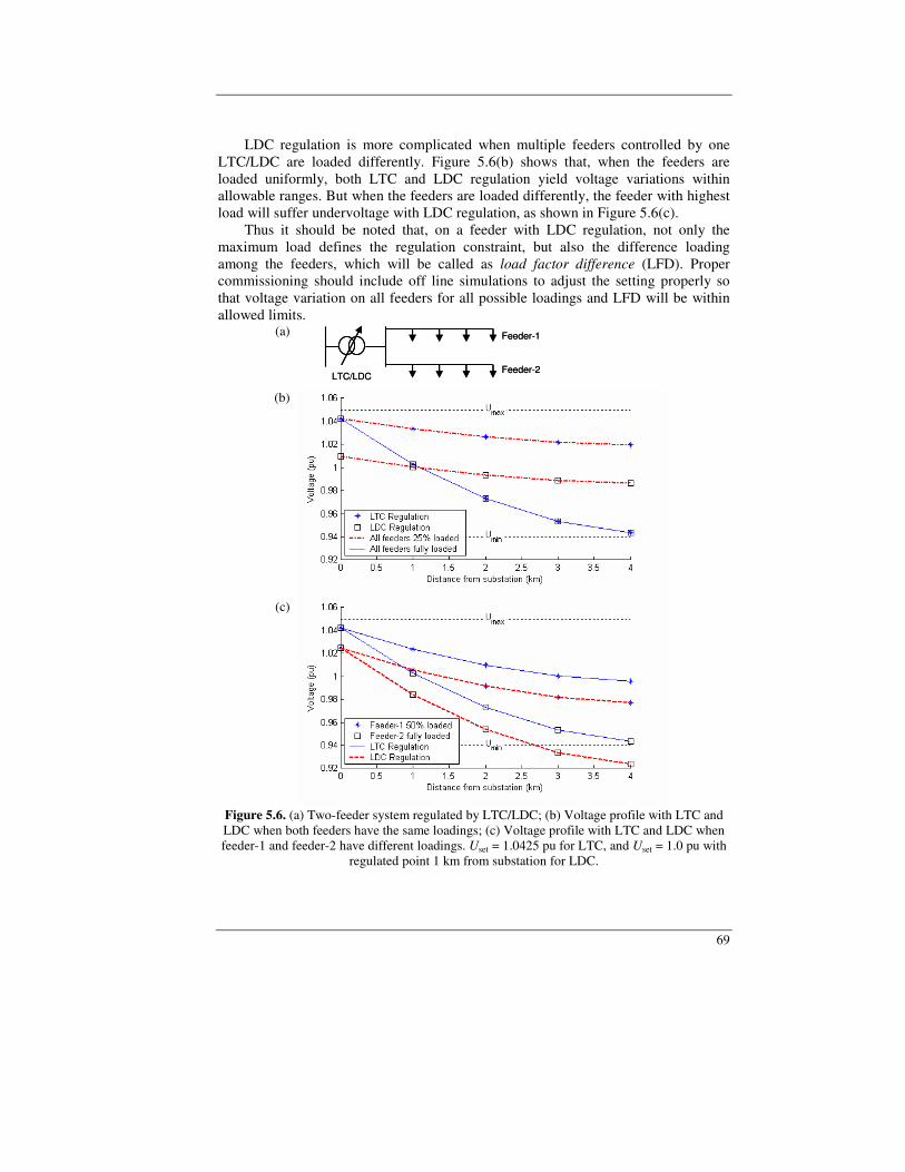
69
LDC regulation is more complicated when multiple feeders controlled by one LTC/LDC are loaded differently. Figure 5.6(b) shows that, when the feeders are loaded uniformly, both LTC and LDC regulation yield voltage variations within allowable ranges. But when the feeders are loaded differently, the feeder with highest load will suffer undervoltage with LDC regulation, as shown in Figure 5.6(c). Thus it should be noted that, on a feeder with LDC regulation, not only the maximum load defines the regulation constraint, but also the difference loading among the feeders, which will be called as load factor difference (LFD). Proper commissioning should include off line simulations to adjust the setting properly so that voltage variation on all feeders for all possible loadings and LFD will be within allowed limits.
(a)
(b)
(c)
Feeder-1
Feeder-2LTC/LDC
Feeder-1
Feeder-2LTC/LDC
Figure 5.6. (a) Two-feeder system regulated by LTC/LDC; (b) Voltage profile with LTC and LDC when both feeders have the same loadings; (c) Voltage profile with LTC and LDC when feeder-1 and feeder-2 have different loadings. Uset = 1.0425 pu for LTC, and Uset = 1.0 pu with
regulated point 1 km from substation for LDC.
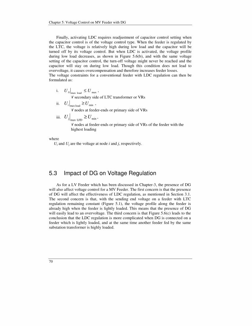
Chapter 5: Voltage Control on MV Feeder with DG
70
Finally, activating LDC requires readjustment of capacitor control setting when the capacitor control is of the voltage control type. When the feeder is regulated by the LTC, the voltage is relatively high during low load and the capacitor will be turned off by its voltage control. But when LDC is activated, the voltage profile during low load decreases, as shown in Figure 5.6(b), and with the same voltage setting of the capacitor control, the turn-off voltage might never be reached and the capacitor will stay on during low load. Though this condition does not lead to overvoltage, it causes overcompensation and therefore increases feeder losses. The voltage constraints for a conventional feeder with LDC regulation can then be formulated as:
i. maxloadmax 0 UU ≤ ,
secondary side of LTC transformer or VRs
ii. minloadmax i UU ≥ ,
nodes at feeder-ends or primary side of VRs
iii. minLFDmax j UU ≥ ,
nodes at feeder-ends or primary side of VRs of the feeder with the highest loading
where Ui and Uj are the voltage at node i and j, respectively.
5.3 Impact of DG on Voltage Regulation
As for a LV Feeder which has been discussed in Chapter-3, the presence of DG will also affect voltage control for a MV Feeder. The first concern is that the presence of DG will affect the effectiveness of LDC regulation, as mentioned in Section 3.1. The second concern is that, with the sending end voltage on a feeder with LTC regulation remaining constant (Figure 5.1), the voltage profile along the feeder is already high when the feeder is lightly loaded. This means that the presence of DG will easily lead to an overvoltage. The third concern is that Figure 5.6(c) leads to the conclusion that the LDC regulation is more complicated when DG is connected on a feeder which is lightly loaded, and at the same time another feeder fed by the same substation transformer is highly loaded.

71
5.3.1 DG Connection to Feeder with LTC Regulation As explained in Section 5.2.1, the performance of LTC regulation is not affected by changes in pf or the direction of active/reactive power, and, for multi-feeder systems, each feeder can be treated individually. This means that only the voltage rise at the DG connection point and its impact on the voltage profile of the particular feeder where DG is connected need to be considered. Voltage constraints for LTC regulated feeder with DG can then be formulated as:
i. max0 UU ≤ , secondary side of LTC transformer or VRs
ii. minDG no load,max i UU ≥ , nodes at feeder-ends or primary side of VRs
iii. maxDGmax load,min DG UU ≤
where Ui is the voltage at node i. Other constraints are conductor ampacity Imax and transformer rating STX. To obtain safe results, one should take as reference UUB when the limiting factor is Umax, and ULB when the limiting factor is Umin, Imax or STX. The linear voltage drop/rise approximation for a simplified feeder with one load and one DG at LC
DG
LGL0DG
)(U
QXPPRUU LL +−−= (5-13)
indicates that the DG integration limit can be increased by lowering the sending-end voltage U0. On the other hand, the current will increase when U0 decreases, which means that the ampacity constraint could be violated. However, the effect on the voltage profile is more significant. One drawback of LTC regulation is that the DG integration limit is relatively low, especially for DG connection far away from the substation. LTC keeps the sending-end voltage constant, which causes the voltage along the feeder to be high when the feeder is lightly loaded, so there is very little margin before the power produced by DG causes overvoltage.
5.3.2 DG Connection to Feeder with LDC Regulation As explained in Section 5.2.2, LDC is affected by changes in pf and by power direction reversal, which can occur due to DG connection.

Chapter 5: Voltage Control on MV Feeder with DG
72
Equation (5-9) is still valid, with I being the net current flow due to the combined effect of load and DG. Rewriting Eq.(5-9) using the net active power (PL-PDG), it can easily be concluded that a low value of PDG, less than about twice the load power, will decrease the net active power flow and thereby reduces the error due to poorly adjusted X/R of the setting. On the other hand, the pf also decreases, which counteracts the error reduction. For higher values of PDG, the error will increase as compared to the conventional feeder and with the increase of DG power. Moreover, while DG operating at unity pf will have the beneficial effect of increasing the overall pf, the situation is aggravated if the DG operates at leading pf, which should be avoided. Similar to the case of the capacitor shown in Figure 5.5, DG connected between LTC and LC will alter the current and pf seen at the LTC and thereby introduces an error. This situation can be more serious than in the case of the capacitor, since the capacitor is normally smaller than the total reactive power consumed by loads, while the DG can in principle be larger than the total load. The regulated point should in this case be moved upstream the DG connection point. DG will also worsen the voltage variations among the feeders with different loading when it is connected to the feeder with the lowest load. In this particular case, a solution can be to move the regulated point closer to the source (with appropriate adjustment of Uset). Thus, on feeders with LDC regulation, DG will not only affect the voltage profile on the feeder where it is connected, but will also cause more voltage drop on adjacent feeders, and decrease the sending-end voltage U0 when the load is minimum and the DG is maximum. The voltage constraints for a LDC regulated feeder with DG can then be formulated as:
i. maxDG no load, max0 UU ≤ ,
secondary side of LTC transformer or VRs ii. minDG no ,load maxi UU ≥ ,
nodes at feeder-ends or primary side of VRs
iii. minLFDmax j UU ≥ ,
nodes at feeder-ends or primary side of VRs of the feeder with the highest loading
iv. minDGmax ,LFD maxk UU ≥ ,
nodes at feeder-ends or primary side of VRs of the feeder with the highest loading, with DG connected on the feeder with lowest loading
v. minDGmax load,min 0 UU ≥
vi. maxDGmax load,min DG UU ≤
where Ui, Uj and Uk are the voltage at node i, j and k, respectively.
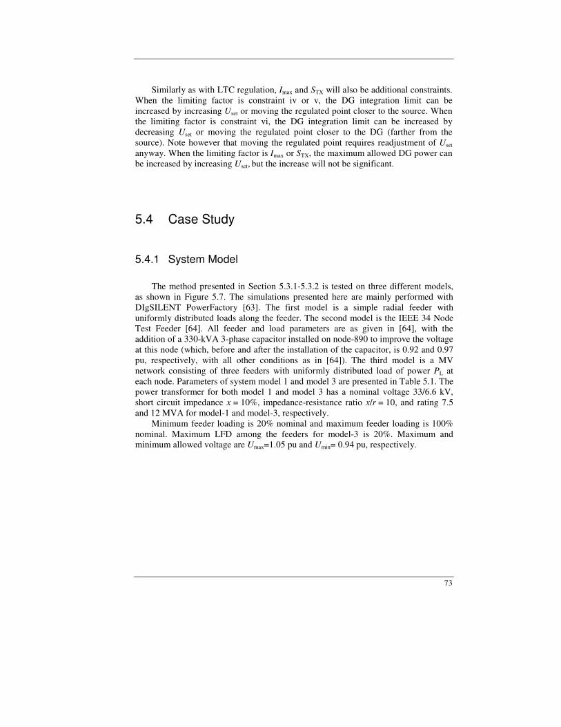
73
Similarly as with LTC regulation, Imax and STX will also be additional constraints. When the limiting factor is constraint iv or v, the DG integration limit can be increased by increasing Uset or moving the regulated point closer to the source. When the limiting factor is constraint vi, the DG integration limit can be increased by decreasing Uset or moving the regulated point closer to the DG (farther from the source). Note however that moving the regulated point requires readjustment of Uset anyway. When the limiting factor is Imax or STX, the maximum allowed DG power can be increased by increasing Uset, but the increase will not be significant.
5.4 Case Study
5.4.1 System Model The method presented in Section 5.3.1-5.3.2 is tested on three different models, as shown in Figure 5.7. The simulations presented here are mainly performed with DIgSILENT PowerFactory [63]. The first model is a simple radial feeder with uniformly distributed loads along the feeder. The second model is the IEEE 34 Node Test Feeder [64]. All feeder and load parameters are as given in [64], with the addition of a 330-kVA 3-phase capacitor installed on node-890 to improve the voltage at this node (which, before and after the installation of the capacitor, is 0.92 and 0.97 pu, respectively, with all other conditions as in [64]). The third model is a MV network consisting of three feeders with uniformly distributed load of power PL at each node. Parameters of system model 1 and model 3 are presented in Table 5.1. The power transformer for both model 1 and model 3 has a nominal voltage 33/6.6 kV, short circuit impedance x = 10%, impedance-resistance ratio x/r = 10, and rating 7.5 and 12 MVA for model-1 and model-3, respectively. Minimum feeder loading is 20% nominal and maximum feeder loading is 100% nominal. Maximum LFD among the feeders for model-3 is 20%. Maximum and minimum allowed voltage are Umax=1.05 pu and Umin= 0.94 pu, respectively.
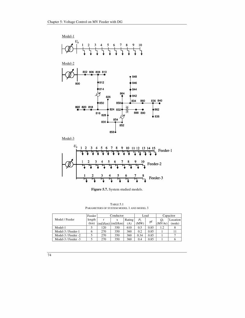
Chapter 5: Voltage Control on MV Feeder with DG
74
Model-1
1 2 3 4 5 6 7 8 9 10U0
1 2 3 4 5 6 7 8 9 10U0
Model-2
800
806 808 810
812
802
824
826
814
850
816
822 820 818
828
830
856
832888 890
838
862
836860834
842
844
846
848
864
858
854
852
840
800
806 808 810
812
802
824
826
814
850
816
822 820 818822 820 818
828
830
856
832888 890
838
862
836860834
842
844
846
848
864
858
854
852
840
Model-3
Feeder-21 2 3 4 5 6 7 8 9 10
Feeder-11 2 3 4 5 6 7 8 9 10 11 12 13 14 15
Feeder-31 2 3 4 5 6 7 8
U0
Feeder-21 2 3 4 5 6 7 8 9 101 2 3 4 5 6 7 8 9 10
Feeder-11 2 3 4 5 6 7 8 9 10 11 12 13 14 151 2 3 4 5 6 7 8 9 10 11 12 13 14 15
Feeder-31 2 3 4 5 6 7 81 2 3 4 5 6 7 8
U0
Figure 5.7. System studied models.
TABLE 5.1 PARAMETERS OF SYSTEM MODEL 1 AND MODEL 3
Conductor Load Capacitor
Model / Feeder Feeder length (km)
r (m/km)
x (m/km)
Rating (A)
PL (MW) pf QC
(MVAr) Location (node)
Model-1 5 120 350 610 0.5 0.85 1.2 8 Model-3 / Feeder-1 6 270 350 360 0.2 0.85 1 11 Model-3 / Feeder -2 5 270 350 360 0.34 0.85 1 7 Model-3 / Feeder -3 5 270 350 360 0.4 0.85 1 6
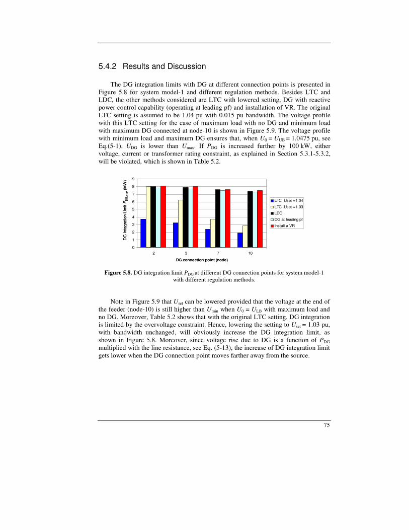
75
5.4.2 Results and Discussion The DG integration limits with DG at different connection points is presented in Figure 5.8 for system model-1 and different regulation methods. Besides LTC and LDC, the other methods considered are LTC with lowered setting, DG with reactive power control capability (operating at leading pf) and installation of VR. The original LTC setting is assumed to be 1.04 pu with 0.015 pu bandwidth. The voltage profile with this LTC setting for the case of maximum load with no DG and minimum load with maximum DG connected at node-10 is shown in Figure 5.9. The voltage profile with minimum load and maximum DG ensures that, when U0 = UUB = 1.0475 pu, see Eq.(5-1), UDG is lower than Umax. If PDG is increased further by 100 kW, either voltage, current or transformer rating constraint, as explained in Section 5.3.1-5.3.2, will be violated, which is shown in Table 5.2.
0
1
2
3
4
5
6
7
8
9
2 3 7 10
DG connection point (node)
LTC, Uset =1.04
LTC, Uset =1.03
LDC
DG at leading pf
Install a VR
DG
Inte
grat
ion
Lim
it P
DG
,max
(MW
)
0
1
2
3
4
5
6
7
8
9
2 3 7 10
DG connection point (node)
LTC, Uset =1.04
LTC, Uset =1.03
LDC
DG at leading pf
Install a VR
DG
Inte
grat
ion
Lim
it P
DG
,max
(MW
)
Figure 5.8. DG integration limit PDG at different DG connection points for system model-1
with different regulation methods.
Note in Figure 5.9 that Uset can be lowered provided that the voltage at the end of the feeder (node-10) is still higher than Umin when U0 = ULB with maximum load and no DG. Moreover, Table 5.2 shows that with the original LTC setting, DG integration is limited by the overvoltage constraint. Hence, lowering the setting to Uset = 1.03 pu, with bandwidth unchanged, will obviously increase the DG integration limit, as shown in Figure 5.8. Moreover, since voltage rise due to DG is a function of PDG
multiplied with the line resistance, see Eq. (5-13), the increase of DG integration limit gets lower when the DG connection point moves farther away from the source.
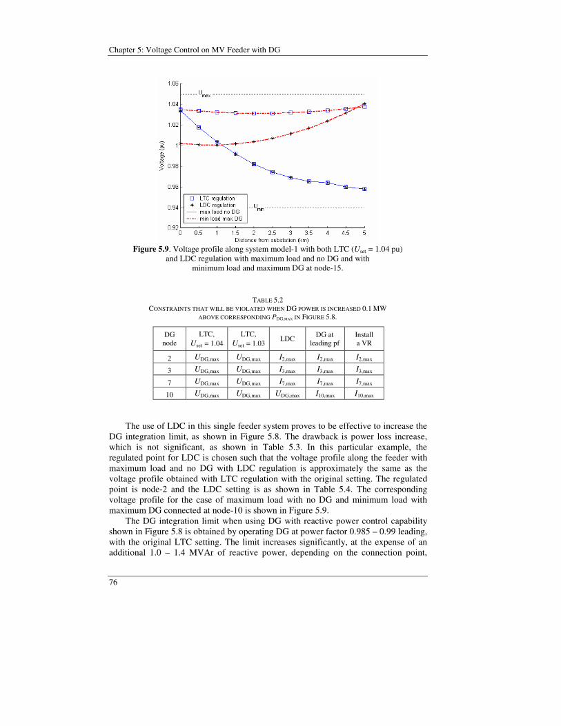
Chapter 5: Voltage Control on MV Feeder with DG
76
Figure 5.9. Voltage profile along system model-1 with both LTC (Uset = 1.04 pu)
and LDC regulation with maximum load and no DG and with minimum load and maximum DG at node-15.
TABLE 5.2 CONSTRAINTS THAT WILL BE VIOLATED WHEN DG POWER IS INCREASED 0.1 MW
ABOVE CORRESPONDING PDG,MAX IN FIGURE 5.8.
DG node
LTC, Uset = 1.04
LTC, Uset = 1.03
LDC DG at leading pf
Install a VR
2 UDG,max UDG,max I2,max I2,max I2,max
3 UDG,max UDG,max I3,max I3,max I3,max
7 UDG,max UDG,max I7,max I7,max I7,max
10 UDG,max UDG,max UDG,max I10,max I10,max The use of LDC in this single feeder system proves to be effective to increase the DG integration limit, as shown in Figure 5.8. The drawback is power loss increase, which is not significant, as shown in Table 5.3. In this particular example, the regulated point for LDC is chosen such that the voltage profile along the feeder with maximum load and no DG with LDC regulation is approximately the same as the voltage profile obtained with LTC regulation with the original setting. The regulated point is node-2 and the LDC setting is as shown in Table 5.4. The corresponding voltage profile for the case of maximum load with no DG and minimum load with maximum DG connected at node-10 is shown in Figure 5.9. The DG integration limit when using DG with reactive power control capability shown in Figure 5.8 is obtained by operating DG at power factor 0.985 – 0.99 leading, with the original LTC setting. The limit increases significantly, at the expense of an additional 1.0 – 1.4 MVAr of reactive power, depending on the connection point,
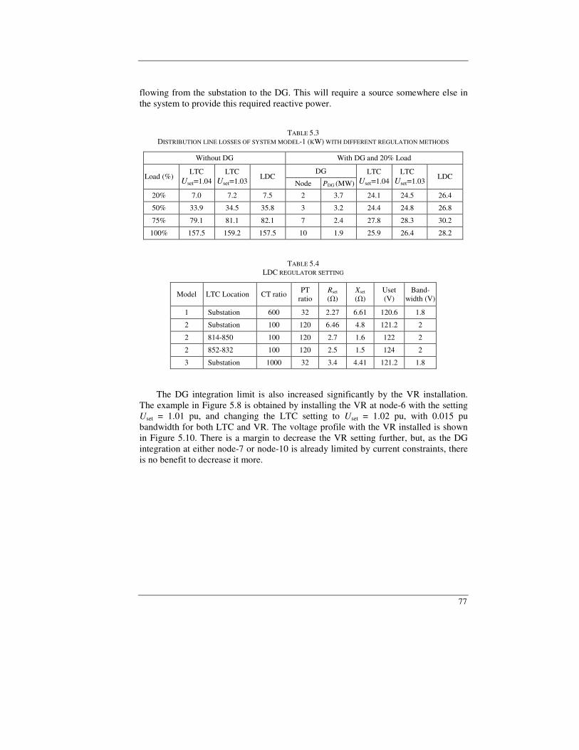
77
flowing from the substation to the DG. This will require a source somewhere else in the system to provide this required reactive power.
TABLE 5.3
DISTRIBUTION LINE LOSSES OF SYSTEM MODEL-1 (KW) WITH DIFFERENT REGULATION METHODS
Without DG With DG and 20% Load
DG Load (%)
LTC Uset=1.04
LTC Uset=1.03
LDC Node PDG (MW)
LTC Uset=1.04
LTC Uset=1.03
LDC
20% 7.0 7.2 7.5 2 3.7 24.1 24.5 26.4
50% 33.9 34.5 35.8 3 3.2 24.4 24.8 26.8
75% 79.1 81.1 82.1 7 2.4 27.8 28.3 30.2
100% 157.5 159.2 157.5 10 1.9 25.9 26.4 28.2
TABLE 5.4 LDC REGULATOR SETTING
Model LTC Location CT ratio PT ratio
Rset ()
Xset ()
Uset (V)
Band-width (V)
1 Substation 600 32 2.27 6.61 120.6 1.8
2 Substation 100 120 6.46 4.8 121.2 2
2 814-850 100 120 2.7 1.6 122 2
2 852-832 100 120 2.5 1.5 124 2
3 Substation 1000 32 3.4 4.41 121.2 1.8 The DG integration limit is also increased significantly by the VR installation. The example in Figure 5.8 is obtained by installing the VR at node-6 with the setting Uset = 1.01 pu, and changing the LTC setting to Uset = 1.02 pu, with 0.015 pu bandwidth for both LTC and VR. The voltage profile with the VR installed is shown in Figure 5.10. There is a margin to decrease the VR setting further, but, as the DG integration at either node-7 or node-10 is already limited by current constraints, there is no benefit to decrease it more.

Chapter 5: Voltage Control on MV Feeder with DG
78
the voltage is stepped up/down by the VR
the voltage is stepped up/down by the VR
Figure 5.10. Voltage profile along the system model-1 with VR installation at node-6
(Uset = 1.02 pu for the LTC and Uset = 1.01 pu for the VR). The DG integration limits for system model-2 with different regulation methods are presented in Figure 5.11. The constraints that will be violated when further increasing PDG by 100 kW are presented in Table 5.5. Compared with system model-1, this model has a lower voltage drop during maximum load. Therefore, the LTC setting can be decreased until 1.02 pu to allow higher DG integration. For the case of DG with reactive power control capability, the limit is obtained by limiting the minimum power factor of the DG to 0.90. The VR is installed at node-808 with setting 1.01 pu. After installation of this VR, the regulator settings are 1.00 pu for the LTC and 1.02 for both VRs at 850-814 and at 852-832. The increase in DG integration limit by operating DG at leading power factor in this model is shown to be less effective than it is in system model-1. The main reason is that the line in system model-2 has a much higher resistance than in system model-1. The impact of line resistance on the effectiveness of reactive power control with DG to limit voltage rise due to DG has already been shown in Chapter 3.
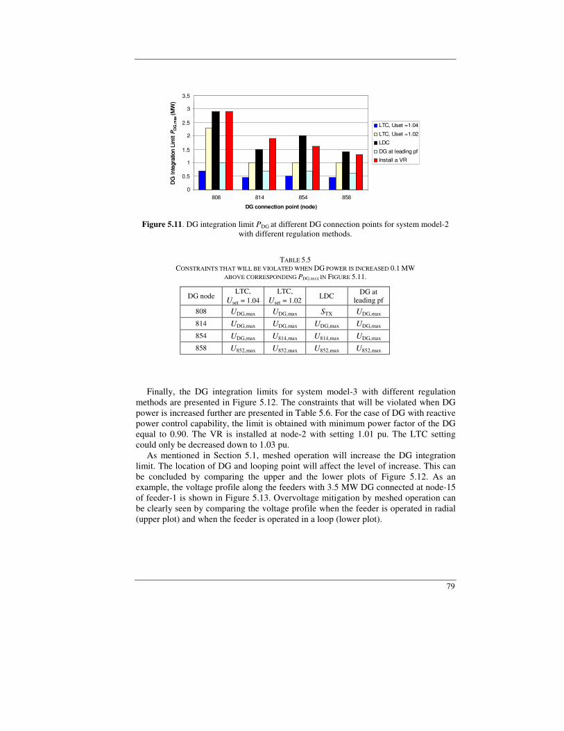
79
0
0,5
1
1,5
2
2,5
3
3,5
808 814 854 858
DG connection point (node)
LTC, Uset =1.04
LTC, Uset =1.02
LDC
DG at leading pf
Install a VR
3.5
2.5
1.5
0.5D
G In
tegr
atio
n Li
mit
PD
G,m
ax(M
W)
0
0,5
1
1,5
2
2,5
3
3,5
808 814 854 858
DG connection point (node)
LTC, Uset =1.04
LTC, Uset =1.02
LDC
DG at leading pf
Install a VR
3.5
2.5
1.5
0.5D
G In
tegr
atio
n Li
mit
PD
G,m
ax(M
W)
Figure 5.11. DG integration limit PDG at different DG connection points for system model-2
with different regulation methods.
TABLE 5.5 CONSTRAINTS THAT WILL BE VIOLATED WHEN DG POWER IS INCREASED 0.1 MW
ABOVE CORRESPONDING PDG,MAX IN FIGURE 5.11.
DG node LTC,
Uset = 1.04 LTC,
Uset = 1.02 LDC DG at
leading pf 808 UDG,max UDG,max STX UDG,max 814 UDG,max UDG,max UDG,max UDG,max 854 UDG,max U814,max U814,max UDG,max 858 U852,max U852,max U852,max U852,max
Finally, the DG integration limits for system model-3 with different regulation methods are presented in Figure 5.12. The constraints that will be violated when DG power is increased further are presented in Table 5.6. For the case of DG with reactive power control capability, the limit is obtained with minimum power factor of the DG equal to 0.90. The VR is installed at node-2 with setting 1.01 pu. The LTC setting could only be decreased down to 1.03 pu. As mentioned in Section 5.1, meshed operation will increase the DG integration limit. The location of DG and looping point will affect the level of increase. This can be concluded by comparing the upper and the lower plots of Figure 5.12. As an example, the voltage profile along the feeders with 3.5 MW DG connected at node-15 of feeder-1 is shown in Figure 5.13. Overvoltage mitigation by meshed operation can be clearly seen by comparing the voltage profile when the feeder is operated in radial (upper plot) and when the feeder is operated in a loop (lower plot).
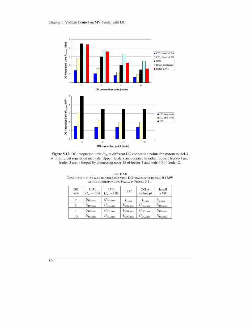
Chapter 5: Voltage Control on MV Feeder with DG
80
0
1
2
3
4
5
3 7 11 15
DG connection point (node)
LTC, Uset =1.04
LTC, Uset =1.03
LDC
DG at leading pf
Install a VRD
G In
tegr
atio
n Li
mit
PD
G,m
ax(M
W)
0
1
2
3
4
5
3 7 11 15
DG connection point (node)
LTC, Uset =1.04
LTC, Uset =1.03
LDC
DG at leading pf
Install a VRD
G In
tegr
atio
n Li
mit
PD
G,m
ax(M
W)
0
1
2
3
4
5
3 7 11 15
DG connection point (node)
LTC, Uset =1.04
LTC, Uset =1.03
LDC
DG
Inte
grat
ion
Lim
it P
DG
,max
(MW
)
0
1
2
3
4
5
3 7 11 15
DG connection point (node)
LTC, Uset =1.04
LTC, Uset =1.03
LDC
DG
Inte
grat
ion
Lim
it P
DG
,max
(MW
)
Figure 5.12. DG integration limit PDG at different DG connection points for system model-3 with different regulation methods. Upper: feeders are operated in radial. Lower: feeder-1 and
feeder-3 are in looped by connecting node-15 of feeder-1 and node-10 of feeder-2.
TABLE 5.6
CONSTRAINTS THAT WILL BE VIOLATED WHEN DG POWER IS INCREASED 0.1 MW ABOVE CORRESPONDING PDG,MAX IN FIGURE 5.11.
DG node
LTC, Uset = 1.04
LTC, Uset = 1.03
LDC DG at leading pf
Install a VR
2 UDG,max UDG,max I3,max I3,max U2,max
3 UDG,max UDG,max UDG,max UDG,max UDG,max
7 UDG,max UDG,max UDG,max UDG,max UDG,max
10 UDG,max UDG,max UDG,max UDG,max UDG,max
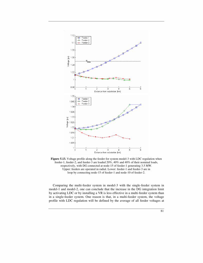
81
Figure 5.13. Voltage profile along the feeder for system model-3 with LDC regulation when
feeder-1, feeder-2, and feeder-3 are loaded 20%, 40% and 40% of their nominal loads, respectively, with DG connected at node-15 of feeder-1 generating 3.5 MW.
Upper: feeders are operated in radial. Lower: feeder-1 and feeder-3 are in loop by connecting node-15 of feeder-1 and node-10 of feeder-2.
Comparing the multi-feeder system in model-3 with the single-feeder system in model-1 and model-2, one can conclude that the increase in the DG integration limit by activating LDC or by installing a VR is less effective in a multi-feeder system than in a single-feeder system. One reason is that, in a multi-feeder system, the voltage profile with LDC regulation will be defined by the average of all feeder voltages at

Chapter 5: Voltage Control on MV Feeder with DG
82
the regulated points. Furthermore, when a VR is installed in a multi-feeder system, the LTC setting cannot be decreased as much as in a single-feeder system, as the decrease will affect the voltage profile on other feeders. After the VR installation, the LTC setting was changed to 1.03 pu in system model-3, compared to 1.02 and 1.00 pu in system model-1 and model-2, respectively.
5.5 Conclusions
In this chapter, voltage regulation in MV feeders with DG has been analyzed. The principle of operation of LTCs with and without LDC has been reviewed and the effect of DG on LTC and LDC regulation has been analyzed. Based on simulations on three different feeder models, the effectiveness of different regulation methods (LTC with reduced setting, LDC, DG with reactive power control capability, VR installation and feeder operation in loop) has been analyzed and is shown to depend on feeder structure, parameters and DG connection point.
It has been demonstrated that the use of LTCs with LDC can significantly increase the maximum size of DG that can be connected to a given feeder without disrupting voltage regulation. By revising the LTC settings and activating the LDC feature, which is present in most LTCs but often not used, connection of DG can be allowed without the need for additional equipment to counteract problems such as voltage rise in low load conditions.
The use of LDC to increase the DG integration limit should be explored as an alternative before e.g. operating DG at leading power factor, which implies additional reactive power flowing from the substation to the DG, and VR installation, which means additional investment cost.
The performance of LDC is affected by changes in the power factor and direction of power flow, which can occur with the installation of DG. However, with a proper commissioning and a set of off-line simulations, it can be ensured that a given size of DG can be connected at a given location without violating the voltage regulation constraints, for all load conditions. It is also indicated that power loss increase due to the use of LDC in MV feeder, with and without DG, is not significant.
Finally, it is shown that meshed operation of feeders will minimize the voltage unbalance among the feeders and increase the DG integration limit.
Chapter 6
Voltage Dip and Overcurrent Protection
in the Presence of Distributed
Generation
This chapter discusses the impact of DG in MV feeders on overcurrent protection in a MV feeder and the voltage dip sensed by LV customers. The voltage dip is coordinated with overcurrent protection and the result is compared to voltage dip immunity of a sensitive equipment (SE) in order to investigate whether the DG will have a role in preventing SE from tripping or not. The chapter firstly investigates voltage dips, short circuit and overcurrent protection in a radial MV distribution network without DG. A distribution model is developed for a study case. DG impact is then investigated based on literature studies and simulations using this developed model.
6.1 Introduction According to the International Electrotechnical Commission (IEC) a voltage dip
is “a sudden reduction of the voltage at a point in the electrical system, followed by a voltage recovery after a short period of time, from half a cycle to a few seconds” [65]. Voltage dip is also called voltage sag, referring to the Institute of Electrical and Electronics Engineers (IEEE), which is defined as “a decrease in rms voltage at the power frequency for durations of 0.5 cycle to 1 minute” [66].
A voltage dip is associated with an occurrence of a short circuit or another extreme increase in current like motor starting or transformer energizing. This thesis focuses on voltage dips caused by short circuits (faults). The dip is characterized by its magnitude and duration, see Figure 6.1. Basically, fault types, source and fault impedances define the dip magnitude, whereas fault clearing time defines the dip duration of a fault-caused dip. Dip magnitude is considered here as the remaining
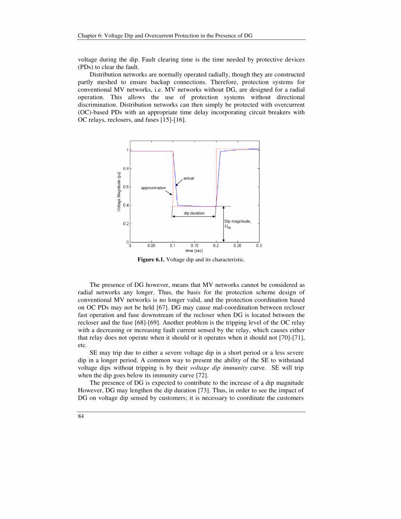
Chapter 6: Voltage Dip and Overcurrent Protection in the Presence of DG
84
voltage during the dip. Fault clearing time is the time needed by protective devices (PDs) to clear the fault. Distribution networks are normally operated radially, though they are constructed partly meshed to ensure backup connections. Therefore, protection systems for conventional MV networks, i.e. MV networks without DG, are designed for a radial operation. This allows the use of protection systems without directional discrimination. Distribution networks can then simply be protected with overcurrent (OC)-based PDs with an appropriate time delay incorporating circuit breakers with OC relays, reclosers, and fuses [15]-[16].
approximation
actual
dip duration
Dip magnitude,Udip
approximation
actual
dip duration
Dip magnitude,Udip
Figure 6.1. Voltage dip and its characteristic.
The presence of DG however, means that MV networks cannot be considered as radial networks any longer. Thus, the basis for the protection scheme design of conventional MV networks is no longer valid, and the protection coordination based on OC PDs may not be held [67]. DG may cause mal-coordination between recloser fast operation and fuse downstream of the recloser when DG is located between the recloser and the fuse [68]-[69]. Another problem is the tripping level of the OC relay with a decreasing or increasing fault current sensed by the relay, which causes either that relay does not operate when it should or it operates when it should not [70]-[71], etc. SE may trip due to either a severe voltage dip in a short period or a less severe dip in a longer period. A common way to present the ability of the SE to withstand voltage dips without tripping is by their voltage dip immunity curve. SE will trip when the dip goes below its immunity curve [72]. The presence of DG is expected to contribute to the increase of a dip magnitude However, DG may lengthen the dip duration [73]. Thus, in order to see the impact of DG on voltage dip sensed by customers; it is necessary to coordinate the customers
85
voltage dip immunity, voltage dip magnitude and fault clearing time performed by the PD, which here will be called as coordination of voltage dip and OC protection.
In [74], the voltage dip in a feeder with DG is coordinated with OC protection in a voltage-time coordinate. The available fault currents are combined with PD’s clearing times to obtain fault clearing times along the feeder. The fault clearing times are plotted against voltage dips sensed by SE to obtain a voltage-time curve of the voltage dip sensed by SE. The curve is then compared with the voltage dip immunity of SE. The limitation of this study is that the coordination of voltage dip and OC protection is based on the coordination of voltage dip with a single PD and is focused on how the PD clearing time should be set to prevent SE from tripping. However, a feeder may consist of several PDs in series, where the PDs have to be selected in such way that all the PDs in series perform a proper protection coordination. Thus, it is necessary to include the OC protection coordination in the coordination of voltage dip and OC protection. This chapter discusses the impact of DG in MV feeders on OC protection in MV feeder, the voltage dip sensed by LV customers, and analyzes how the DG will prevent the LV customers from tripping. Potential problems and solutions to OC protection coordination in MV feeders with a high penetration of DG are investigated. The coordination of voltage dip and OC protection is presented in a time-current curve (TCC), by taking into account proper protection coordination in the feeder. The presentation of voltage dip and OC protection in a TCC is intended to give a better overview of how the TCC of the PD should be, in order to prevent the LV customers from tripping.
6.2 Short Circuit and Voltage Dip Magnitude on A Radial Feeder
Consider a MV network with a balanced three-phase fault at feeder-1 and SE connected at the LV side of feeder-2 through a Dy transformer in Figure 6.2. Assume that the initial voltage behind the source impedance is 1.0 pu as shown in the equivalent diagram in Figure 6.3, the short circuit current IF, in per unit, will be
FS,1SS,1
1ZZ
IF += (6-1)
where Z1,SS and Z1,FS are the positive sequence impedances at source side and at fault side, respectively. Neglecting the fault current contribution from loads, the voltage dip at SE connection point, Udip, on a balanced three-phase fault is equal to the dip at the primary side of Dy transformer (see Figure 6.3), which is also equal to the voltage at the point of common coupling (PCC). The voltage dip, in per unit, is then given by

Chapter 6: Voltage Dip and Overcurrent Protection in the Presence of DG
86
PCCdip UU = (6-2)
FS,1SS,1
FS,1PCC ZZ
ZU
+= (6-3)
Grid
Dy
PCC
IF
SE
Feeder-2
Feeder-1
Grid
Dy
PCC
IF
SE
Feeder-2
Feeder-1
Figure 6.2. A simple radial circuit for fault and voltage dip studies.
Z1,SS Z1,FS
UPCC1 pu+
IF
+
Z1,SS Z1,FS
UPCC1 pu+
IF
+
Figure 6.3. Short circuit and voltage dip diagram for three phase balance faults.
The short circuit current and the voltage dip at PCC for unbalanced faults can be calculated by means of sequence voltages, currents and impedances. The phase currents and voltages are related to the sequence currents and voltages with the following transformations [75]-[76]:
=
2
1
0
2
2
c
b
a
11
111
I
II
I
II
αααα (6-4)
=
2
1
0
2
2
c
b
a
11
111
U
U
U
U
U
U
αααα (6-5)
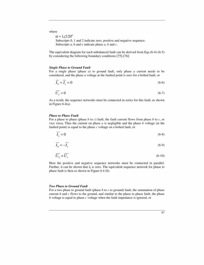
87
where o1201∠=α
Subscripts 0, 1 and 2 indicate zero, positive and negative sequence. Subscripts a, b and c indicate phase a, b and c.
The equivalent diagram for each unbalanced fault can be derived from Eqs.(6-4)-(6-5) by considering the following boundary conditions [75]-[76]: Single Phase to Ground Fault For a single phase (phase a) to ground fault, only phase a current needs to be considered, and the phase a voltage at the faulted point is zero for a bolted fault, or
0cb == II (6-6)
0a =U (6-7)
As a result, the sequence networks must be connected in series for this fault, as shown in Figure 6.4(a). Phase to Phase Fault For a phase to phase (phase b to c) fault, the fault current flows from phase b to c, or vice versa. Thus the current on phase a is negligible and the phase b voltage (at the faulted point) is equal to the phase c voltage on a bolted fault, or
0a =I (6-8)
cb II −= (6-9)
cb UU = (6-10)
Here the positive and negative sequence networks must be connected in parallel. Further, it can be shown that I0 is zero. The equivalent sequence network for phase to phase fault is then as shown in Figure 6.4 (b). Two Phase to Ground Fault For a two phase to ground fault (phase b to c to ground) fault, the summation of phase current b and c flows to the ground, and similar to the phase to phase fault, the phase b voltage is equal to phase c voltage when the fault impedance is ignored, or
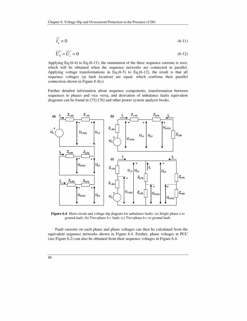
Chapter 6: Voltage Dip and Overcurrent Protection in the Presence of DG
88
0a =I (6-11)
0cb == UU (6-12)
Applying Eq.(6-4) to Eq.(6-11), the summation of the three sequence currents is zero, which will be obtained when the sequence networks are connected in parallel. Applying voltage transformations in Eq.(6-5) to Eq.(6-12), the result is that all sequence voltages (at fault location) are equal, which confirms their parallel connection shown in Figure 6.4(c). Further detailed information about sequence components, transformation between sequences to phases and vice versa, and derivation of unbalance faults equivalent diagrams can be found in [75]-[76] and other power system analysis books.
(c)
Z1,SS Z1,FS
U1,PCC U1,FUin
+
(b)(a)
Uin
+
I1 I2I1
I2
I0
+ + ++ +
+ +
+ +
Uin
+
I0
+ +
++
+
Z1,FS Z2,FS
Z1,SS
Z2,SS
U1,PCC
U1,F U2,F
U2,PCC
Z2,SS Z2,FS
U2,PCC U2,F
Z0,SS Z0,FS
U0,PCC U0,F
Z1,SS
Z1,FS
I1
U1,PCC
U1,F U2,F
Z2,FS
Z2,SS
I2
U2,PCC
U0,F
U0,PCC
Z0,FS
Z0,SS
(c)
Z1,SS Z1,FS
U1,PCC U1,FUin
+
(b)(a)
Uin
+
I1 I2I1
I2
I0
+ + ++ +
+ +
+ +
Uin
+
I0
+ +
++
+
Z1,FS Z2,FS
Z1,SS
Z2,SS
U1,PCC
U1,F U2,F
U2,PCC
Z2,SS Z2,FS
U2,PCC U2,F
Z0,SS Z0,FS
U0,PCC U0,F
Z1,SS
Z1,FS
I1
U1,PCC
U1,F U2,F
Z2,FS
Z2,SS
I2
U2,PCC
U0,F
U0,PCC
Z0,FS
Z0,SS
Figure 6.4. Short circuit and voltage dip diagram for unbalance faults: (a) Single phase a to ground fault; (b) Two-phase b-c fault; (c) Two-phase b-c to ground fault.
Fault currents on each phase and phase voltages can then be calculated from the equivalent sequence networks shown in Figure 6.4. Further, phase voltages at PCC (see Figure 6.2) can also be obtained from their sequence voltages in Figure 6.4.
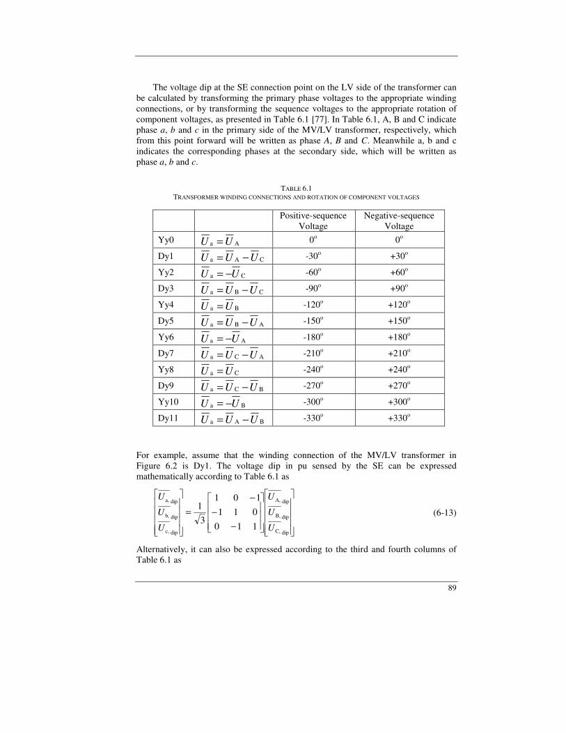
89
The voltage dip at the SE connection point on the LV side of the transformer can be calculated by transforming the primary phase voltages to the appropriate winding connections, or by transforming the sequence voltages to the appropriate rotation of component voltages, as presented in Table 6.1 [77]. In Table 6.1, A, B and C indicate phase a, b and c in the primary side of the MV/LV transformer, respectively, which from this point forward will be written as phase A, B and C. Meanwhile a, b and c indicates the corresponding phases at the secondary side, which will be written as phase a, b and c.
TABLE 6.1 TRANSFORMER WINDING CONNECTIONS AND ROTATION OF COMPONENT VOLTAGES
Positive-sequence Voltage
Negative-sequence Voltage
Yy0 Aa UU = 0o 0o
Dy1 CAa UUU −= -30o +30o
Yy2 Ca UU −= -60o +60o
Dy3 CBa UUU −= -90o +90o
Yy4 Ba UU = -120o +120o
Dy5 ABa UUU −= -150o +150o
Yy6 Aa UU −= -180o +180o
Dy7 ACa UUU −= -210o +210o
Yy8 Ca UU = -240o +240o
Dy9 BCa UUU −= -270o +270o
Yy10 Ba UU −= -300o +300o
Dy11 BAa UUU −= -330o +330o For example, assume that the winding connection of the MV/LV transformer in Figure 6.2 is Dy1. The voltage dip in pu sensed by the SE can be expressed mathematically according to Table 6.1 as
−−
−=
dipC,
dipB,
dipA,
dipc,
dipb,
dipa,
110011101
31
U
U
U
U
U
U (6-13)
Alternatively, it can also be expressed according to the third and fourth columns of Table 6.1 as
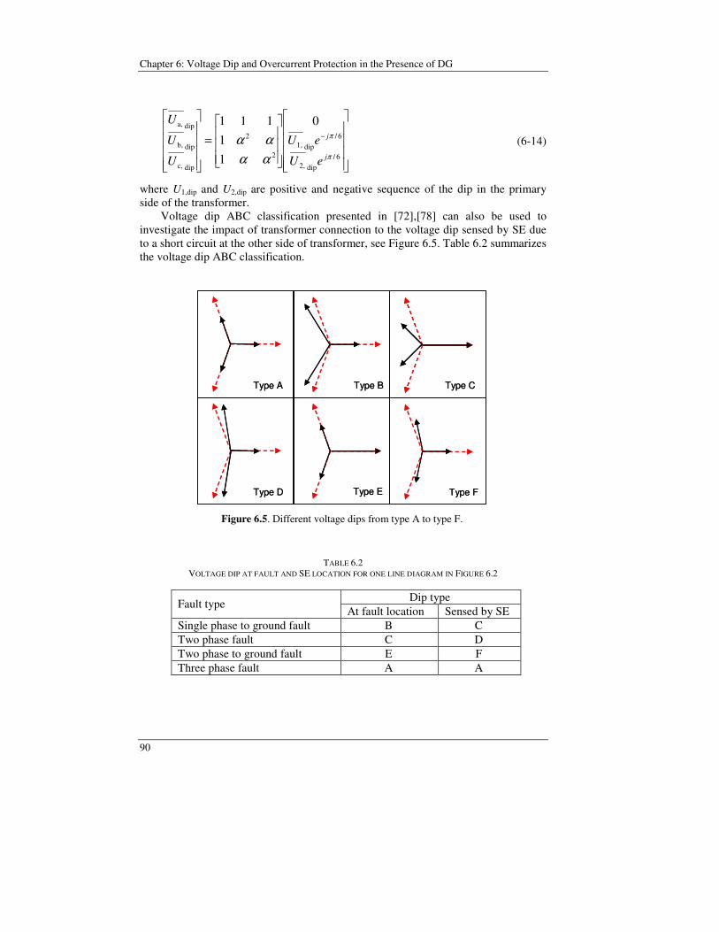
Chapter 6: Voltage Dip and Overcurrent Protection in the Presence of DG
90
=
−
6/dip2,
6/dip1,
2
2
dipc,
dipb,
dipa, 0
11
111
π
π
αααα
j
j
eU
eU
U
U
U (6-14)
where U1,dip and U2,dip are positive and negative sequence of the dip in the primary side of the transformer.
Voltage dip ABC classification presented in [72],[78] can also be used to investigate the impact of transformer connection to the voltage dip sensed by SE due to a short circuit at the other side of transformer, see Figure 6.5. Table 6.2 summarizes the voltage dip ABC classification.
Type A
Type D
Type B Type C
Type E Type F
Type A
Type D
Type B Type C
Type E Type F
Figure 6.5. Different voltage dips from type A to type F.
TABLE 6.2 VOLTAGE DIP AT FAULT AND SE LOCATION FOR ONE LINE DIAGRAM IN FIGURE 6.2
Dip type Fault type
At fault location Sensed by SE Single phase to ground fault B C Two phase fault C D Two phase to ground fault E F Three phase fault A A
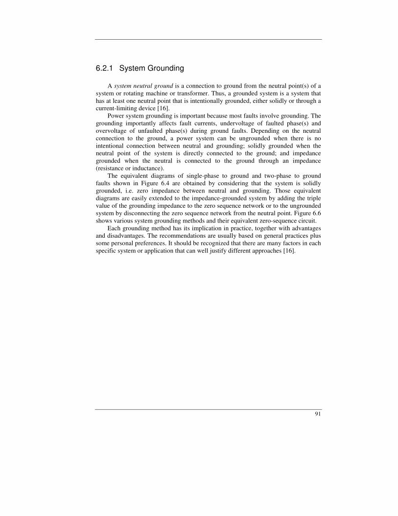
91
6.2.1 System Grounding A system neutral ground is a connection to ground from the neutral point(s) of a system or rotating machine or transformer. Thus, a grounded system is a system that has at least one neutral point that is intentionally grounded, either solidly or through a current-limiting device [16]. Power system grounding is important because most faults involve grounding. The grounding importantly affects fault currents, undervoltage of faulted phase(s) and overvoltage of unfaulted phase(s) during ground faults. Depending on the neutral connection to the ground, a power system can be ungrounded when there is no intentional connection between neutral and grounding; solidly grounded when the neutral point of the system is directly connected to the ground; and impedance grounded when the neutral is connected to the ground through an impedance (resistance or inductance). The equivalent diagrams of single-phase to ground and two-phase to ground faults shown in Figure 6.4 are obtained by considering that the system is solidly grounded, i.e. zero impedance between neutral and grounding. Those equivalent diagrams are easily extended to the impedance-grounded system by adding the triple value of the grounding impedance to the zero sequence network or to the ungrounded system by disconnecting the zero sequence network from the neutral point. Figure 6.6 shows various system grounding methods and their equivalent zero-sequence circuit. Each grounding method has its implication in practice, together with advantages and disadvantages. The recommendations are usually based on general practices plus some personal preferences. It should be recognized that there are many factors in each specific system or application that can well justify different approaches [16].
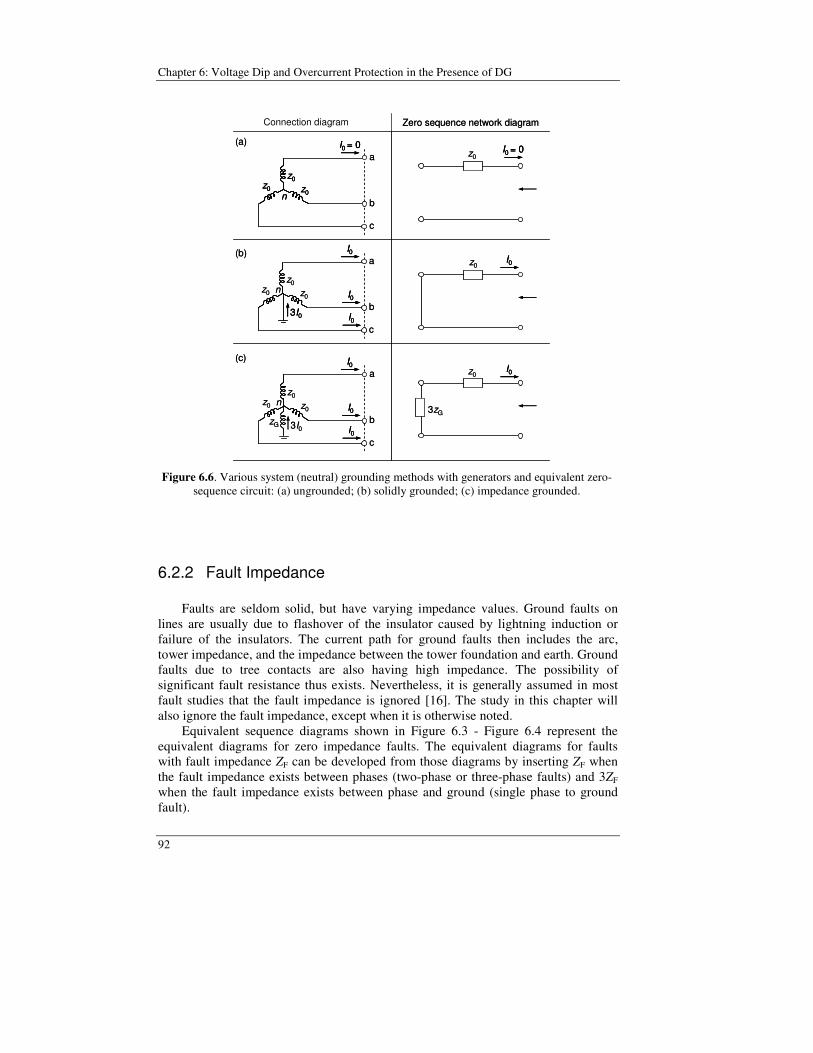
Chapter 6: Voltage Dip and Overcurrent Protection in the Presence of DG
92
a
b
c
I0 = 0
a
b
c
3I0
a
b
c
3I0
3zGzG
(a)
(b)
(c)
Connection diagram Zero sequence network diagram
z0
nz0
z0
z0
z0n z0
z0
I0
I0
I0
I0
I0I0
I0
I0
I0 = 0
z0
z0
z0n z0
z0
a
b
c
I0 = 0I0 = 0
a
b
c
3I03I0
a
b
c
3I0
3zGzG
(a)
(b)
(c)
Connection diagram Zero sequence network diagram
z0
nz0
z0
z0
nz0
z0
z0
z0n z0
z0
I0I0
I0I0
I0I0
I0I0
I0I0I0I0
I0I0
I0I0
I0 = 0I0 = 0
z0
z0
z0n z0
z0
Figure 6.6. Various system (neutral) grounding methods with generators and equivalent zero-
sequence circuit: (a) ungrounded; (b) solidly grounded; (c) impedance grounded.
6.2.2 Fault Impedance Faults are seldom solid, but have varying impedance values. Ground faults on
lines are usually due to flashover of the insulator caused by lightning induction or failure of the insulators. The current path for ground faults then includes the arc, tower impedance, and the impedance between the tower foundation and earth. Ground faults due to tree contacts are also having high impedance. The possibility of significant fault resistance thus exists. Nevertheless, it is generally assumed in most fault studies that the fault impedance is ignored [16]. The study in this chapter will also ignore the fault impedance, except when it is otherwise noted.
Equivalent sequence diagrams shown in Figure 6.3 - Figure 6.4 represent the equivalent diagrams for zero impedance faults. The equivalent diagrams for faults with fault impedance ZF can be developed from those diagrams by inserting ZF when the fault impedance exists between phases (two-phase or three-phase faults) and 3ZF when the fault impedance exists between phase and ground (single phase to ground fault).

93
6.3 Case Study
For further illustration and analysis voltage dip and OC protection coordination in this chapter, 13.8 kV OH distribution feeders supplied from a 115 kV line through a 115/13.8 kV transformer are used. The typical one line diagram of protection systems and load connections of the feeder is shown in Figure 6.10. The protections and load connections of two other feeders are similar, but different, which are not shown here.
SubstationTransformer
Grid
R
R
A
A
Cus
tom
ers
Transformer fuse
Distribution Transformer
Recloser
Linefuse
Breaker with OC relays
SubstationTransformer
Grid
R
R
A
AA
Cus
tom
ers
Transformer fuse
Distribution Transformer
Recloser
Linefuse
Breaker with OC relays
Figure 6.7. Typical one line diagram of protection systems and
load connections for the case study.
Based on typical protections and load connections in Figure 6.10, a model shown in Figure 6.8 is developed. LV customers connecting to feeder-2 (see Figure 6.8) are of interest for voltage dip analysis. The distribution transformer is protected by transformer fuse but not shown in the figure in order not to make any confusion with line fuses. Indeed, this chapter will only focus on faults on MV lines, in which the transformer fuse does not have any role. The connection of LV customers to the LV feeder is shown in Figure 6.9. Figure 6.8 - Figure 6.9 will be used extensively for the case model in this chapter.
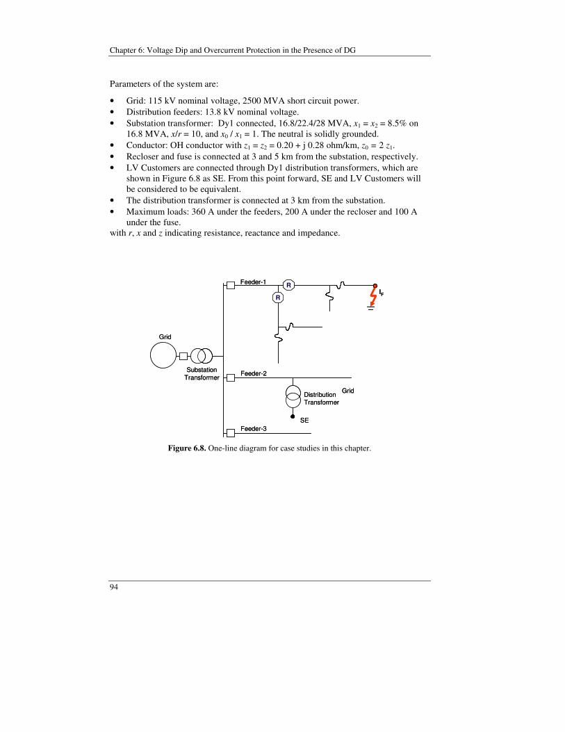
Chapter 6: Voltage Dip and Overcurrent Protection in the Presence of DG
94
Parameters of the system are:
• Grid: 115 kV nominal voltage, 2500 MVA short circuit power. • Distribution feeders: 13.8 kV nominal voltage. • Substation transformer: Dy1 connected, 16.8/22.4/28 MVA, x1 = x2 = 8.5% on
16.8 MVA, x/r = 10, and x0 / x1 = 1. The neutral is solidly grounded. • Conductor: OH conductor with z1 = z2 = 0.20 + j 0.28 ohm/km, z0 = 2 z1. • Recloser and fuse is connected at 3 and 5 km from the substation, respectively. • LV Customers are connected through Dy1 distribution transformers, which are
shown in Figure 6.8 as SE. From this point forward, SE and LV Customers will be considered to be equivalent.
• The distribution transformer is connected at 3 km from the substation. • Maximum loads: 360 A under the feeders, 200 A under the recloser and 100 A
under the fuse. with r, x and z indicating resistance, reactance and impedance.
SE
Feeder-1
Feeder-2
IF
Feeder-3
SubstationTransformer
Distribution Transformer
Grid
R
R
Grid
SE
Feeder-1
Feeder-2
IFIF
Feeder-3
SubstationTransformer
Distribution Transformer
Grid
R
R
Grid
Figure 6.8. One-line diagram for case studies in this chapter.

95
13.8 kV
3-phaseprimary
4-wire, 3-phase secondary, 220/380 V
Customers
DistributionTransformer 13.8 kV
3-phaseprimary
4-wire, 3-phase secondary, 220/380 V
Customers
DistributionTransformer
Figure 6.9. Three-phase diagram of customer connection to the LV Feeder.
Fault currents and phase voltages (at substation 13.8 kV bus) as a function of fault location, for bolted faults, are shown in Figure 6.10 and Figure 6.11, respectively. For simplicity, the fault currents due to two-phase to ground faults are not shown in Figure 6.10, as this fault results in different fault current magnitudes flowing on the faulted phases and neutral. The two-phase to ground faults will also not be analyzed further. The three-phase fault current is shown to be 2/3 times the corresponding two-phase fault current. This is because the negative sequence impedance for the whole system is equal to that of the positive sequence.
As explained before, the voltage dip due to a three phase fault sensed by LV customers, at any phases they are connected to, is equal to the voltage at Substation 13.8 kV bus.
Figure 6.10. Fault currents as a function of fault locations for different faults types.

Chapter 6: Voltage Dip and Overcurrent Protection in the Presence of DG
96
UA, UB, UC3-phase faults
UA1-phase faults
UB2-phase faults
UC2-phase faults
UB2-phase to ground faults
UC2-phase to ground faults
UA, UB, UC3-phase faults
UA1-phase faults
UB2-phase faults
UC2-phase faults
UB2-phase to ground faults
UC2-phase to ground faults
Figure 6.11. Voltage at substation 13.8 kV Bus as a function of fault locations for different
faults types (phase A to ground, phase B to C, phase B to C to ground, and phase A to B to C). The notation “UA 1-phase faults”, for instance,
means voltage dips at phase A due to 1-phase faults.
Voltage dips sensed by LV customers due to 2-phase (phase B to C) faults in
feeder-1 are shown in Figure 6.12. As can be concluded from Figure 6.5 and Table 6.2, the two-phase faults will cause voltage dips on all three phases at the secondary side of a Dy transformer. When the customers are connected to phase voltages; the customers connected to phase c will suffer a severe voltage dip, as severe as voltage dip due to a corresponding three-phase fault; whereas the customers connected to phase a and b will experience less severe voltage dip. When the customers are connected to line voltages; the customers connected to phase a-b do not feel any voltage dip at all.
Voltage dips sensed by LV customers due to single-phase (phase A) to ground faults in feeder-1 are shown in Figure 6.13. The single-phase to ground fault is sensed as a two phase voltage dip by the LV customers, as can also be concluded from Figure 6.5 and Table 6.2. The customers connected to phase a (to neutral) will not feel the voltage dip. When the LV customers are connected to line voltages, the customers connected to phase a-b will suffer a severe voltage dip.
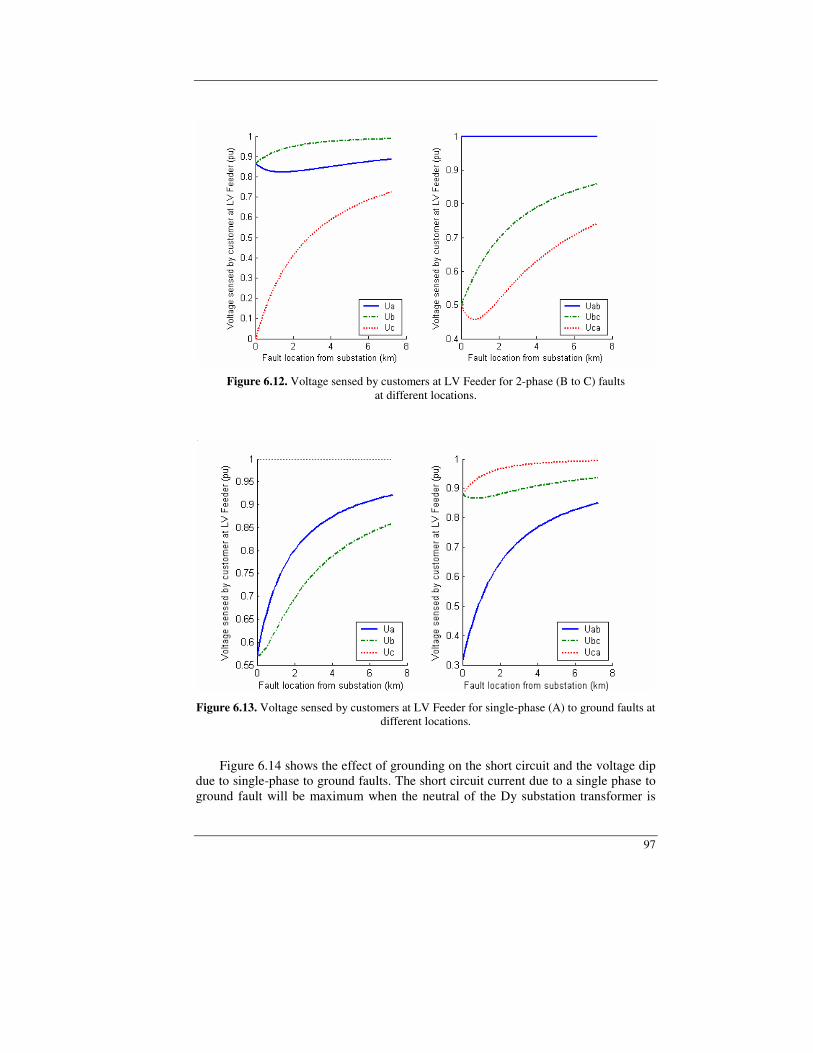
97
Figure 6.12. Voltage sensed by customers at LV Feeder for 2-phase (B to C) faults
at different locations.
Figure 6.13. Voltage sensed by customers at LV Feeder for single-phase (A) to ground faults at different locations.
Figure 6.14 shows the effect of grounding on the short circuit and the voltage dip due to single-phase to ground faults. The short circuit current due to a single phase to ground fault will be maximum when the neutral of the Dy substation transformer is
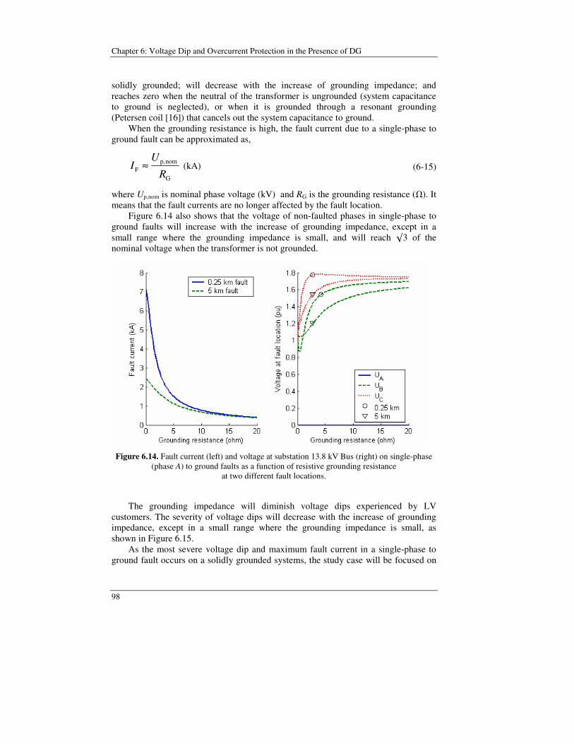
Chapter 6: Voltage Dip and Overcurrent Protection in the Presence of DG
98
solidly grounded; will decrease with the increase of grounding impedance; and reaches zero when the neutral of the transformer is ungrounded (system capacitance to ground is neglected), or when it is grounded through a resonant grounding (Petersen coil [16]) that cancels out the system capacitance to ground. When the grounding resistance is high, the fault current due to a single-phase to ground fault can be approximated as,
G
nomp,F R
UI ≈ (kA) (6-15)
where Up,nom is nominal phase voltage (kV) and RG is the grounding resistance (). It means that the fault currents are no longer affected by the fault location. Figure 6.14 also shows that the voltage of non-faulted phases in single-phase to ground faults will increase with the increase of grounding impedance, except in a small range where the grounding impedance is small, and will reach 3 of the nominal voltage when the transformer is not grounded.
Figure 6.14. Fault current (left) and voltage at substation 13.8 kV Bus (right) on single-phase
(phase A) to ground faults as a function of resistive grounding resistance at two different fault locations.
The grounding impedance will diminish voltage dips experienced by LV customers. The severity of voltage dips will decrease with the increase of grounding impedance, except in a small range where the grounding impedance is small, as shown in Figure 6.15. As the most severe voltage dip and maximum fault current in a single-phase to ground fault occurs on a solidly grounded systems, the study case will be focused on
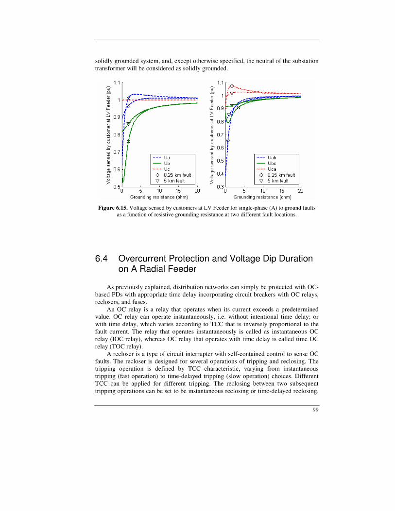
99
solidly grounded system, and, except otherwise specified, the neutral of the substation transformer will be considered as solidly grounded.
Figure 6.15. Voltage sensed by customers at LV Feeder for single-phase (A) to ground faults
as a function of resistive grounding resistance at two different fault locations.
6.4 Overcurrent Protection and Voltage Dip Duration on A Radial Feeder
As previously explained, distribution networks can simply be protected with OC-based PDs with appropriate time delay incorporating circuit breakers with OC relays, reclosers, and fuses. An OC relay is a relay that operates when its current exceeds a predetermined value. OC relay can operate instantaneously, i.e. without intentional time delay; or with time delay, which varies according to TCC that is inversely proportional to the fault current. The relay that operates instantaneously is called as instantaneous OC relay (IOC relay), whereas OC relay that operates with time delay is called time OC relay (TOC relay). A recloser is a type of circuit interrupter with self-contained control to sense OC faults. The recloser is designed for several operations of tripping and reclosing. The tripping operation is defined by TCC characteristic, varying from instantaneous tripping (fast operation) to time-delayed tripping (slow operation) choices. Different TCC can be applied for different tripping. The reclosing between two subsequent tripping operations can be set to be instantaneous reclosing or time-delayed reclosing.
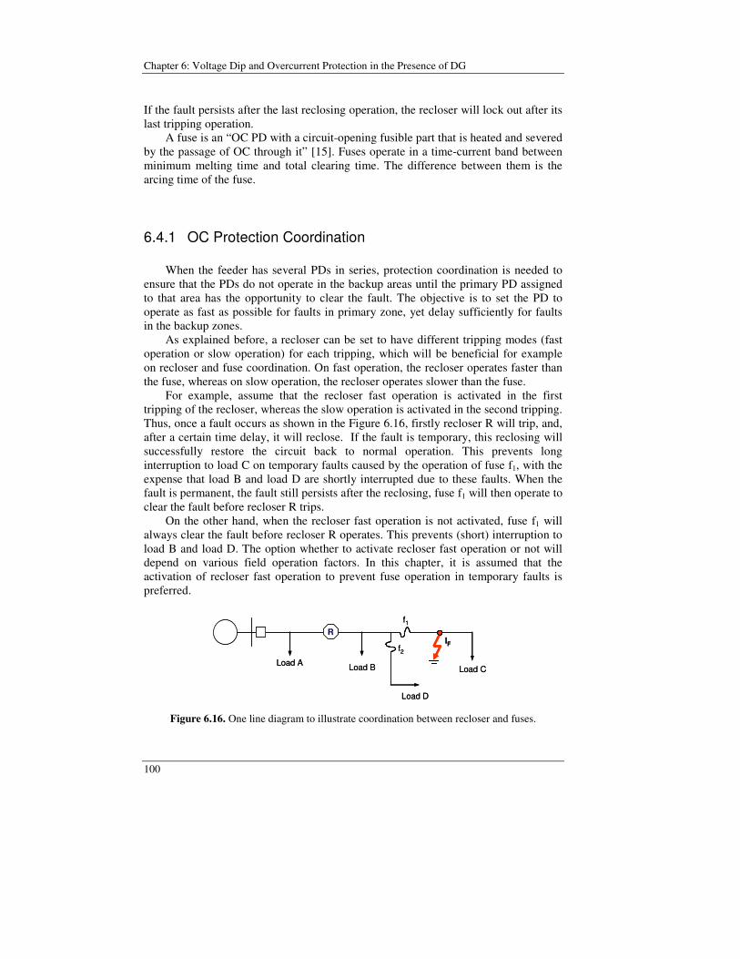
Chapter 6: Voltage Dip and Overcurrent Protection in the Presence of DG
100
If the fault persists after the last reclosing operation, the recloser will lock out after its last tripping operation. A fuse is an “OC PD with a circuit-opening fusible part that is heated and severed by the passage of OC through it” [15]. Fuses operate in a time-current band between minimum melting time and total clearing time. The difference between them is the arcing time of the fuse.
6.4.1 OC Protection Coordination When the feeder has several PDs in series, protection coordination is needed to ensure that the PDs do not operate in the backup areas until the primary PD assigned to that area has the opportunity to clear the fault. The objective is to set the PD to operate as fast as possible for faults in primary zone, yet delay sufficiently for faults in the backup zones.
As explained before, a recloser can be set to have different tripping modes (fast operation or slow operation) for each tripping, which will be beneficial for example on recloser and fuse coordination. On fast operation, the recloser operates faster than the fuse, whereas on slow operation, the recloser operates slower than the fuse.
For example, assume that the recloser fast operation is activated in the first tripping of the recloser, whereas the slow operation is activated in the second tripping. Thus, once a fault occurs as shown in the Figure 6.16, firstly recloser R will trip, and, after a certain time delay, it will reclose. If the fault is temporary, this reclosing will successfully restore the circuit back to normal operation. This prevents long interruption to load C on temporary faults caused by the operation of fuse f1, with the expense that load B and load D are shortly interrupted due to these faults. When the fault is permanent, the fault still persists after the reclosing, fuse f1 will then operate to clear the fault before recloser R trips. On the other hand, when the recloser fast operation is not activated, fuse f1 will always clear the fault before recloser R operates. This prevents (short) interruption to load B and load D. The option whether to activate recloser fast operation or not will depend on various field operation factors. In this chapter, it is assumed that the activation of recloser fast operation to prevent fuse operation in temporary faults is preferred.
RIF
Load A Load B
f1
f2
Load C
Load D
RIFIF
Load A Load B
f1
f2
Load C
Load D Figure 6.16. One line diagram to illustrate coordination between recloser and fuses.

101
With maximum short circuit currents at various locations as shown in Table 6.3, protection coordination on feeder-1 of the case model in Figure 6.8 can be developed as shown in Figure 6.17.
TABLE 6.3 MAXIMUM SHORT CIRCUIT CURRENTS AT VARIOUS FAULT LOCATIONS [KA]
Fault Type Fault Location Three-phase Single-Phase
Relay 7.7 7.9 Reclosers 4.0 3.4
Fuses 3.0 2.5 Furthers-end of the line 2.3 1.9
The fuse and recloser curves are adapted from those in CYMTCC [79], and the relay’s curves are based on IEEE Standard Very Inverse OC Relay in [80] given by the formula
( )
+
−= 491.0
1/61.19
2PU
D IIttop
(6-16)
where top is operating time. tD is time dial. IPU is pickup current. 125A rated fuses are selected for the protection of lateral. The fuse starts operate at around 240A, more than double of the maximum load, which is enough to override the cold load. A 100A rated fuse is also enough to override the cold load, but the fuse needs to be coordinated with recloser fast operation, which can not maintained when a 100A fuse is used. As fuse can not differentiate phase and ground faults, the 125A rated fuses will protect both phase and ground faults. Reclosers are assumed to be conventional reclosers, which have limited option of TCCs [81]. It is shown that the fuse and the recloser can coordinate in a certain range of fault current only. However, the fuse and the recloser coordinate properly for any possible bolted faults downstream the fuse (which is noted as y1 for the fault at furthest end of the feeder, and y2 for the fault at fuse terminal), with sufficient margins to cover high impedance faults. The margin for coordination between the fuse minimum melting time and the recloser tripping time is very narrow, especially for bolted faults occurring immediately downstream of the fuse. This is taken as a compromise to prevent fuse overrating. Though, a better decision either to have narrow coordination (between fuse and recloser fast) or overrating the fuse can be obtained from the fault history of the system. The use of microprocessor type reclosers with much more options of TCC
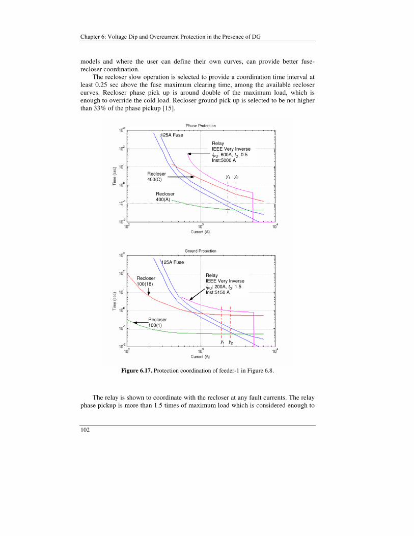
Chapter 6: Voltage Dip and Overcurrent Protection in the Presence of DG
102
models and where the user can define their own curves, can provide better fuse-recloser coordination. The recloser slow operation is selected to provide a coordination time interval at least 0.25 sec above the fuse maximum clearing time, among the available recloser curves. Recloser phase pick up is around double of the maximum load, which is enough to override the cold load. Recloser ground pick up is selected to be not higher than 33% of the phase pickup [15].
RelayIEEE Very InverseIPU: 600A, tD: 0.5Inst:5000 A
125A Fuse
Recloser400(A)
Recloser400(C)
y1 y2
Recloser100(1)
Recloser100(18)
125A Fuse
RelayIEEE Very InverseIPU: 200A, tD: 1.5Inst:5150 A
y1 y2
RelayIEEE Very InverseIPU: 600A, tD: 0.5Inst:5000 A
125A Fuse
Recloser400(A)
Recloser400(C)
y1 y2
Recloser100(1)
Recloser100(18)
125A Fuse
RelayIEEE Very InverseIPU: 200A, tD: 1.5Inst:5150 A
y1 y2
Figure 6.17. Protection coordination of feeder-1 in Figure 6.8.
The relay is shown to coordinate with the recloser at any fault currents. The relay phase pickup is more than 1.5 times of maximum load which is considered enough to
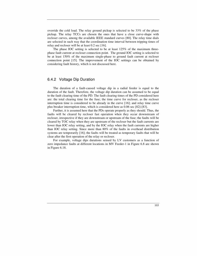
103
override the cold load. The relay ground pickup is selected to be 33% of the phase pickup. The relay TCCs are chosen the ones that have a close curve-shape with recloser curves, among the available IEEE standard curves [80]. The relay time dials are selected in such way that the coordination time interval between tripping times of relay and recloser will be at least 0.2 sec [16]. The phase IOC setting is selected to be at least 125% of the maximum three-phase fault current at recloser connection point. The ground IOC setting is selected to be at least 150% of the maximum single-phase to ground fault current at recloser connection point [15]. The improvement of the IOC settings can be obtained by considering fault history, which is not discussed here.
6.4.2 Voltage Dip Duration
The duration of a fault-caused voltage dip in a radial feeder is equal to the duration of the fault. Therefore, the voltage dip duration can be assumed to be equal to the fault clearing time of the PD. The fault clearing times of the PD considered here are: the total clearing time for the fuse; the time curve for recloser, as the recloser interruption time is considered to be already in the curve [16]; and relay time curve plus breaker interruption time, which is considered here as 0.06 sec [82]-[83].
Further, it is assumed here that the PDs operate properly as they should. Thus, the faults will be cleared by recloser fast operation when they occur downstream of recloser, irrespective if they are downstream or upstream of the fuse; the faults will be cleared by TOC relay when they are upstream of the recloser but the fault currents are lower than IOC relay setting, and by the IOC relay when the fault currents are higher than IOC relay setting. Since more than 80% of the faults in overhead distribution systems are temporarily [16]; the faults will be treated as temporary faults that will be clear after the first operation of the relay or recloser.
For example, voltage dips durations sensed by LV customers as a function of zero impedance faults at different locations in MV Feeder-1 in Figure 6.8 are shown in Figure 6.18.
Chapter 6: Voltage Dip and Overcurrent Protection in the Presence of DG
104
Figure 6.18. Duration of voltage dips sensed by LV customers as a function of zero impedance faults at different locations in MV Feeder-1 in the case study, for three different types of fault.
6.5 Effect of Voltage Dip on Sensitive Equipment Examples of SE are IT equipment, contactors and adjustable-speed drives. IT equipment requires regulated direct current (dc) supply. These supplies are obtained by converting the alternating current (ac) from a power supply into non regulated dc supply, and converting the non regulated dc supply to a regulated dc output. If the ac supply drops, the non regulated dc supply does, too. However, the voltage regulator is able to keep the regulated dc output constant over a certain range of input voltage. But, if the non regulated dc supply becomes too low, the regulated dc output will start to drop and ultimately errors will occur in the digital electronics. As explained before, a common way to presents the ability of the SE to withstand voltage dips without tripping is by presenting their voltage dip immunity curve. A well known voltage dip immunity curve for computers and microprocessor based equipment is issued by the Computer Business Equipment Manufacturing Association (CBEMA). CBEMA curve is used in IEEE Standard 1346 and became a kind of reference for equipment voltage tolerance as well as for severity of voltage dip [72]. However, different sources draw the CBEMA curve differently, for examples as presented in [72], [84] and many online sources such as in [85]. Nowadays, the revised of CBEMA curve has been issued by the Information Technology Industrial Council (ITIC), the successor of CBEMA.

105
Contactors are a very common way of connecting motor load to the supply. The supply voltage is used to power an electromagnet which keeps the contact in place. When the voltage fails or drops the contacts open, preventing the motor from suddenly restarting when the supply voltage comes back. This works fine for example in a long interruption where an unexpected motor starting can be very dangerous. Adjustable speed drives can trip by a voltage dip due to several phenomena, such as [72]: • The drive controller or protection detects the sudden change in operating
conditions and trip the drive to prevent damage to the power electronics components.
• The drop in dc bus voltage, which results from the voltage dip will cause maloperation or tripping of the drive controller or of the PWM inverter.
• The increased ac currents during the dips will cause an OC trip or blowing of fuses protecting the power electronics components. In this thesis, the CBEMA curve presented in [84] will be used to represent the
voltage dip immunity of SE. However, the method presented in this chapter is also applicable to other SE immunity curves.
Further, for quantitative analysis, the CBEMA curve will be approximated analytically as [84]:
( ) =− 287 Ut constant , U < 87 (6-17)
where t is time in cycle at 60 Hz, U is voltage in percent and the constant is 4400. Figure 6.19 shows the CBEMA curve.
Figure 6.19. Voltage dip immunity curve.

Chapter 6: Voltage Dip and Overcurrent Protection in the Presence of DG
106
6.6 Coordination of Voltage Dip and OC Protection
By coordinating voltage dip and OC protection, it can be seen whether the operation of PD can prevent SE from tripping, due to a dip, or not. Obviously, fault clearing time needs to be as short as possible. However, it sometimes can not be achieved. For example, when there are several PDs in series, the upstream PD needs a certain time delay to give the downstream PDs a chance to clear the fault in their protected area. Even when the PD operates instantaneously, the clearing time is sometimes not short enough to prevent the SE from tripping when the voltage dip magnitude sensed by the SE is very low. For example, Figure 6.18 indicates that SE will sense the voltage dip for 0.07 sec when the fault is cleared by IOC relay, meanwhile Figure 6.19 indicates that the SE will only be able to withstand 50% voltage dip for a duration less than 0.06 sec.
The coordination of voltage dip and OC protection will be presented in a TCC. Fault clearing time tclear is obtained from PD’s clearing time, which is a function of fault current. Voltage dips sensed by SE due to the faults are combined with voltage dip immunity of SE to obtain critical fault clearing time in which the SE is still able to withstand the dip, tcrit. The tcrit and tclear are plotted against fault currents and compared. The coordination is successful to prevent SE from tripping when tcrit is higher than tclear for a certain fault current.
For example, the coordination of voltage dip and overcurrent protection of the study case in Section 6.3 is presented in Figure 6.20. The figure shows that the coordination is successful to prevent SE from tripping for any fault occurs downstream of recloser, where the fault is cleared by recloser fast operation. On the other hand, the SE will always trip when a three-phase fault occurs at any location upstream the recloser, even when the fault is cleared by the IOC relay. For two-phase and single-phase to ground fault upstream the recloser; the fault location and the phase where the SE is connected defines whether the coordination is successful or not.

107
tclear
tcrit
tclear
tclear
tcrit-atcrit-b
tcrit-c
tcrit-bc
tcrit-ca
tcrit-a
tcrit-b
tcrit-ab
tcrit-bc
tclear
tcrit
tclear
tclear
tcrit-atcrit-b
tcrit-c
tcrit-bc
tcrit-ca
tcrit-a
tcrit-b
tcrit-ab
tcrit-bc
recloser TOC relay IOC relay
tclear
tcrit
tclear
tclear
tcrit-atcrit-b
tcrit-c
tcrit-bc
tcrit-ca
tcrit-a
tcrit-b
tcrit-ab
tcrit-bc
tclear
tcrit
tclear
tclear
tcrit-atcrit-b
tcrit-c
tcrit-bc
tcrit-ca
tcrit-a
tcrit-b
tcrit-ab
tcrit-bc
recloser TOC relay IOC relay
Figure 6.20. Coordination of voltage dip sensed by SE and overcurrent protection on feeder-1
of the study model. The notation “tcrit-a” and “tcrit-ab”, for instance, means the critical fault clearing time for the SE connected at phase a (to neutral) and phase a to b, respectively.
The notation “recloser”, ”TOC relay” and “IOC relay” for tclear means fault clearing time of recloser, TOC relay and IOC relay, respectively, which is typical
for all three plots, but only shown in the upper plot.
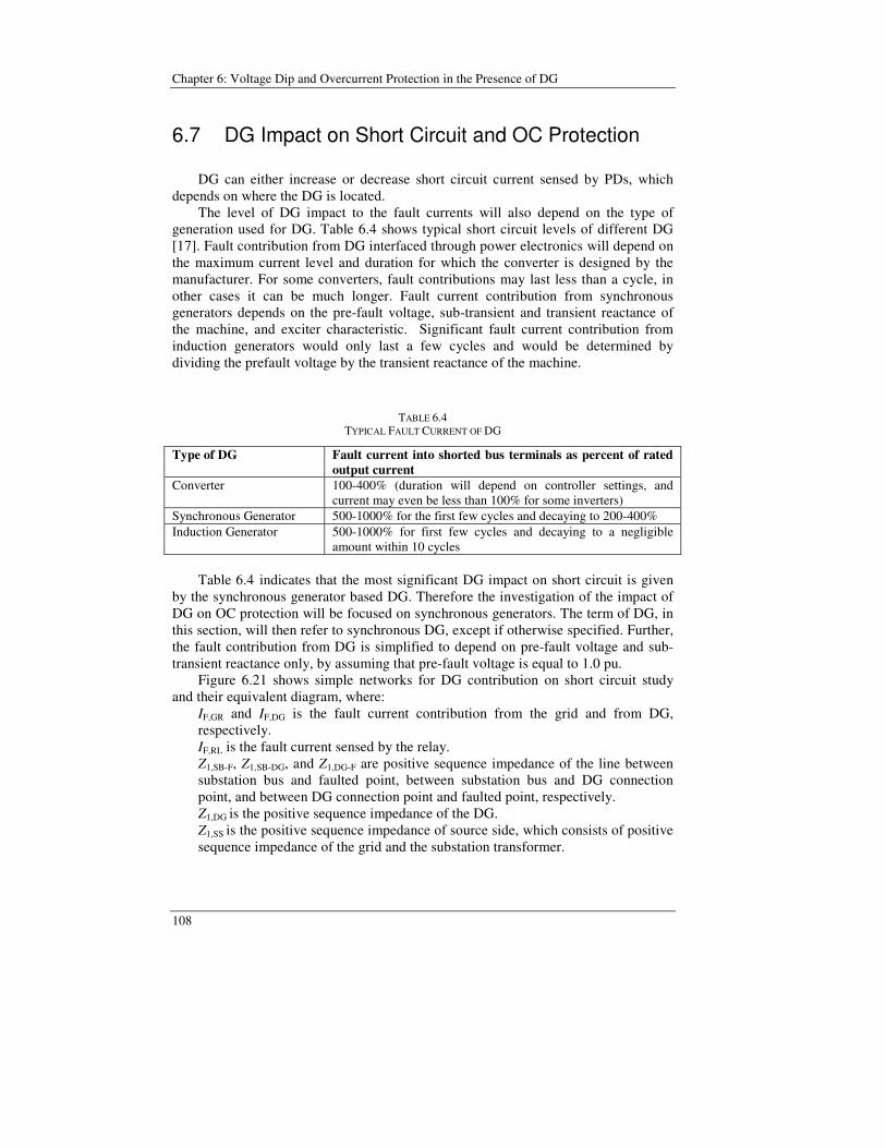
Chapter 6: Voltage Dip and Overcurrent Protection in the Presence of DG
108
6.7 DG Impact on Short Circuit and OC Protection
DG can either increase or decrease short circuit current sensed by PDs, which depends on where the DG is located.
The level of DG impact to the fault currents will also depend on the type of generation used for DG. Table 6.4 shows typical short circuit levels of different DG [17]. Fault contribution from DG interfaced through power electronics will depend on the maximum current level and duration for which the converter is designed by the manufacturer. For some converters, fault contributions may last less than a cycle, in other cases it can be much longer. Fault current contribution from synchronous generators depends on the pre-fault voltage, sub-transient and transient reactance of the machine, and exciter characteristic. Significant fault current contribution from induction generators would only last a few cycles and would be determined by dividing the prefault voltage by the transient reactance of the machine.
TABLE 6.4 TYPICAL FAULT CURRENT OF DG
Type of DG Fault current into shorted bus terminals as percent of rated output current
Converter 100-400% (duration will depend on controller settings, and current may even be less than 100% for some inverters)
Synchronous Generator 500-1000% for the first few cycles and decaying to 200-400% Induction Generator 500-1000% for first few cycles and decaying to a negligible
amount within 10 cycles Table 6.4 indicates that the most significant DG impact on short circuit is given
by the synchronous generator based DG. Therefore the investigation of the impact of DG on OC protection will be focused on synchronous generators. The term of DG, in this section, will then refer to synchronous DG, except if otherwise specified. Further, the fault contribution from DG is simplified to depend on pre-fault voltage and sub-transient reactance only, by assuming that pre-fault voltage is equal to 1.0 pu.
Figure 6.21 shows simple networks for DG contribution on short circuit study and their equivalent diagram, where:
IF,GR and IF,DG is the fault current contribution from the grid and from DG, respectively. IF,RL is the fault current sensed by the relay. Z1,SB-F, Z1,SB-DG, and Z1,DG-F are positive sequence impedance of the line between substation bus and faulted point, between substation bus and DG connection point, and between DG connection point and faulted point, respectively.
Z1,DG is the positive sequence impedance of the DG. Z1,SS is the positive sequence impedance of source side, which consists of positive sequence impedance of the grid and the substation transformer.
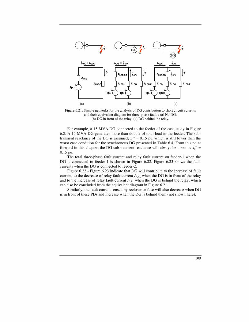
109
z1,SS
z1,SB-DG
z1,DG
+ +1pu 1pu
z1,DG-F
IF,RL = IF,GR
IFIF,DG
z1,SS
+1pu
z1,SB-F
IF,RL = IF,GR
IF
z1,SS
z1,SB-DG
z1,DG
+ +1pu 1pu
z1,SB-F
IF,GR
IFIF,DG
IF,RL
IF IFDGIF
DG
z1,SS
z1,SB-DG
z1,DG
+ +1pu 1pu
z1,DG-F
IF,RL = IF,GR
IFIF,DG
z1,SS
+1pu
z1,SB-F
IF,RL = IF,GR
IF
z1,SS
z1,SB-DG
z1,DG
+ +1pu 1pu
z1,SB-F
IF,GR
IFIF,DG
IF,RL
z1,SS
z1,SB-DG
z1,DG
+ +1pu 1pu
z1,DG-F
IF,RL = IF,GR
IFIF,DG
z1,SS
+1pu
z1,SB-F
IF,RL = IF,GR
IF
z1,SS
z1,SB-DG
z1,DG
+ +1pu 1pu
z1,SB-F
IF,GR
IFIF,DG
IF,RL
IF IFDGIF
DG
IF IFDGIF
DGDG
(a) (b) (c)
Figure 6.21. Simple networks for the analysis of DG contribution to short circuit currents and their equivalent diagram for three-phase faults: (a) No DG;
(b) DG in front of the relay; (c) DG behind the relay.
For example, a 15 MVA DG connected to the feeder of the case study in Figure 6.8. A 15 MVA DG generates more than double of total load in the feeder. The sub-transient reactance of the DG is assumed, xd” = 0.15 pu, which is still lower than the worst case condition for the synchronous DG presented in Table 6.4. From this point forward in this chapter, the DG sub-transient reactance will always be taken as xd” = 0.15 pu.
The total three-phase fault current and relay fault current on feeder-1 when the DG is connected to feeder-1 is shown in Figure 6.22. Figure 6.23 shows the fault currents when the DG is connected to feeder-2.
Figure 6.22 - Figure 6.23 indicate that DG will contribute to the increase of fault current, to the decrease of relay fault current IF,RL when the DG is in front of the relay and to the increase of relay fault current IF,RL when the DG is behind the relay; which can also be concluded from the equivalent diagram in Figure 6.21.
Similarly, the fault current sensed by recloser or fuse will also decrease when DG is in front of these PDs and increase when the DG is behind them (not shown here).
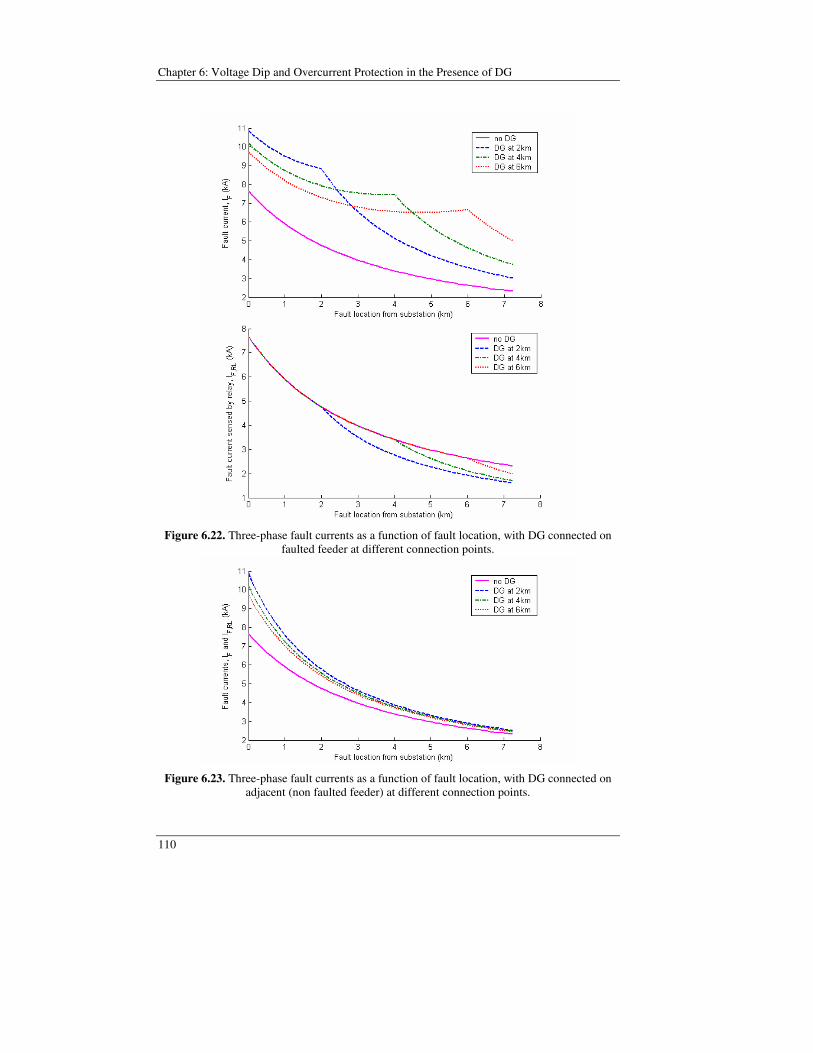
Chapter 6: Voltage Dip and Overcurrent Protection in the Presence of DG
110
Figure 6.22. Three-phase fault currents as a function of fault location, with DG connected on
faulted feeder at different connection points.
Figure 6.23. Three-phase fault currents as a function of fault location, with DG connected on
adjacent (non faulted feeder) at different connection points.
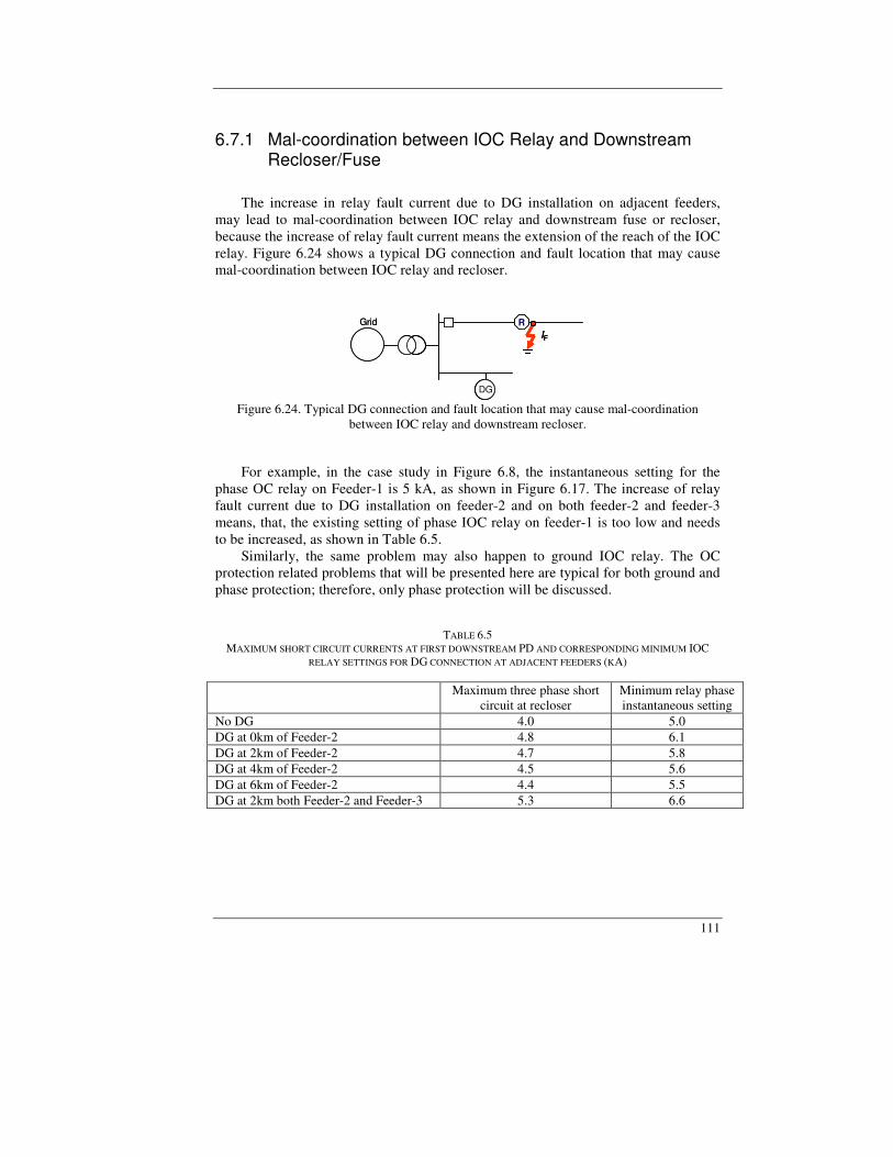
111
6.7.1 Mal-coordination between IOC Relay and Downstream Recloser/Fuse
The increase in relay fault current due to DG installation on adjacent feeders,
may lead to mal-coordination between IOC relay and downstream fuse or recloser, because the increase of relay fault current means the extension of the reach of the IOC relay. Figure 6.24 shows a typical DG connection and fault location that may cause mal-coordination between IOC relay and recloser.
IFGrid R
DG
IFIFGrid R
DGDG Figure 6.24. Typical DG connection and fault location that may cause mal-coordination
between IOC relay and downstream recloser.
For example, in the case study in Figure 6.8, the instantaneous setting for the phase OC relay on Feeder-1 is 5 kA, as shown in Figure 6.17. The increase of relay fault current due to DG installation on feeder-2 and on both feeder-2 and feeder-3 means, that, the existing setting of phase IOC relay on feeder-1 is too low and needs to be increased, as shown in Table 6.5. Similarly, the same problem may also happen to ground IOC relay. The OC protection related problems that will be presented here are typical for both ground and phase protection; therefore, only phase protection will be discussed.
TABLE 6.5 MAXIMUM SHORT CIRCUIT CURRENTS AT FIRST DOWNSTREAM PD AND CORRESPONDING MINIMUM IOC
RELAY SETTINGS FOR DG CONNECTION AT ADJACENT FEEDERS (KA)
Maximum three phase short circuit at recloser
Minimum relay phase instantaneous setting
No DG 4.0 5.0 DG at 0km of Feeder-2 4.8 6.1 DG at 2km of Feeder-2 4.7 5.8 DG at 4km of Feeder-2 4.5 5.6 DG at 6km of Feeder-2 4.4 5.5 DG at 2km both Feeder-2 and Feeder-3 5.3 6.6

Chapter 6: Voltage Dip and Overcurrent Protection in the Presence of DG
112
6.7.2 TOC Relay does not Sense High Impedance Faults
The decrease in relay fault current due to DG installation on the faulted feeder may cause TOC relay not to operate, especially for high impedance faults. Figure 6.25 shows a typical DG connection and fault location that may cause the TOC relay not to sense a high impedance fault.
Grid
DG
IF
Figure 6.25. Typical DG connection that may cause TOC relay not to sense high impedance faults.
The relay fault current (in pu) without DG, see Figure 6.21.(a), for three-phase
faults with fault impedance ZF, can be written as
FF-SB,1SS,1RLF,
1ZZZ
I++
= (6-18)
Meanwhile, if DG is connected to the feeder as in Figure 6.21.(b), the relay fault current will be
( ) ( )( )DG,1DG-SB,1SS,1FF-DG,1DG,1DG-SB,1SS,1
DG,1
RLF,ZZZZZZZZ
ZI
+++++= (6-19)
For example, for the study case in Figure 6.8, the OC relay is supposed to be the
back-up for the recloser, which means that the relay has to reach the end of recloser’s main protected area, i.e. 5 km from substation. The three-phase fault current sensed by the relay, when the fault occurs at 5 km from the substation, as a function of resistive fault impedances, is shown in Figure 6.26. DG, when present, is connected 2 km from the substation. The figure shows that the presence of DG increases the possibility that the relay does not operate for high impedance faults, particularly with the increase of DG size. To mitigate this problem, the pick up current setting of the TOC relay needs to be decreased when DG is present in the feeder.
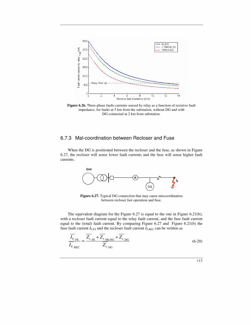
113
Figure 6.26. Three-phase faults currents sensed by relay as a function of resistive fault
impedance, for faults at 5 km from the substation, without DG and with DG connected at 2 km from substation.
6.7.3 Mal-coordination between Recloser and Fuse
When the DG is positioned between the recloser and the fuse, as shown in Figure 6.27, the recloser will sense lower fault currents and the fuse will sense higher fault currents.
Grid
RIF
DG
Grid
RIFIF
DGDG
Figure 6.27. Typical DG connection that may cause miscoordination between recloser fast operation and fuse.
The equivalent diagram for the Figure 6.27 is equal to the one in Figure 6.21(b),
with a recloser fault current equal to the relay fault current, and the fuse fault current equal to the (total) fault current. By comparing Figure 6.27 and Figure 6.21(b) the fuse fault current IF,FS and the recloser fault current IF,REC can be written as
DG1,
DG1,DG-SB1,SS1,
RECF,
FSF,
Z
ZZZ
I
I ++= (6-20)
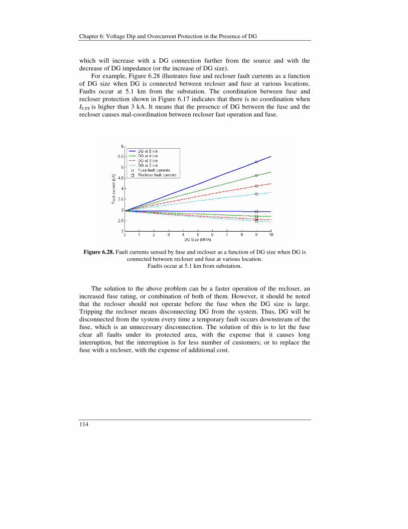
Chapter 6: Voltage Dip and Overcurrent Protection in the Presence of DG
114
which will increase with a DG connection further from the source and with the decrease of DG impedance (or the increase of DG size). For example, Figure 6.28 illustrates fuse and recloser fault currents as a function of DG size when DG is connected between recloser and fuse at various locations. Faults occur at 5.1 km from the substation. The coordination between fuse and recloser protection shown in Figure 6.17 indicates that there is no coordination when IF,FS is higher than 3 kA. It means that the presence of DG between the fuse and the recloser causes mal-coordination between recloser fast operation and fuse.
Figure 6.28. Fault currents sensed by fuse and recloser as a function of DG size when DG is
connected between recloser and fuse at various location. Faults occur at 5.1 km from substation.
The solution to the above problem can be a faster operation of the recloser, an increased fuse rating, or combination of both of them. However, it should be noted that the recloser should not operate before the fuse when the DG size is large. Tripping the recloser means disconnecting DG from the system. Thus, DG will be disconnected from the system every time a temporary fault occurs downstream of the fuse, which is an unnecessary disconnection. The solution of this is to let the fuse clear all faults under its protected area, with the expense that it causes long interruption, but the interruption is for less number of customers; or to replace the fuse with a recloser, with the expense of additional cost.

115
6.7.4 IOC Relay Operates due to Faults on Adjacent Feeders
The increase of DG penetration may cause IOC relay operate due to a fault on an adjacent feeder. Figure 6.29 shows a typical DG connection and fault location that may cause the IOC relay operates due to a fault on an adjacent feeder.
Grid
DG
IF
Grid
DGDG
IFIF
Figure 6.29. Typical DG connection and fault location that may cause IOC relay operate due to faults on an adjacent feeder.
Fault currents sensed by the IOC relay at feeder-1 in Figure 6.8 as a function of
DG size is shown in Figure 6.30. The fault occurs at feeder-2, immediately downstream the breaker. DG is connected at different locations at feeder-1; 0km means that the DG is connected immediately downstream the breaker. Figure 6.30 indicates that, when the DG size in a feeder is high and the DG connection is close to the substation, the IOC relay may operate due a fault at adjacent feeders, especially when the fault is very close to the substation. To mitigate this problem, the setting of the IOC relay needs increasing. Another solution to this problem is the use of directional OC relay, which will be discussed in chapter 7.
Figure 6.30. Fault currents sensed by the IOC relay at feeder-1, due to faults at feeder-2
immediately downstream the breaker, as a function of DG size with DG connected at feeder-1.
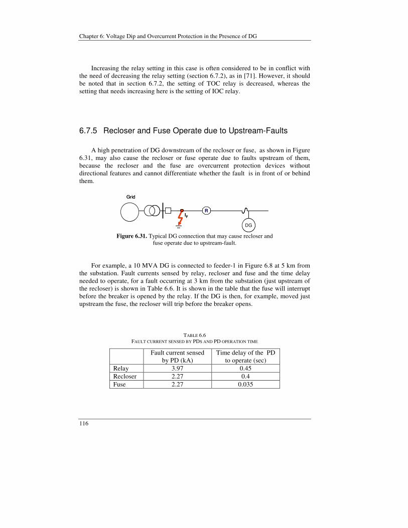
Chapter 6: Voltage Dip and Overcurrent Protection in the Presence of DG
116
Increasing the relay setting in this case is often considered to be in conflict with the need of decreasing the relay setting (section 6.7.2), as in [71]. However, it should be noted that in section 6.7.2, the setting of TOC relay is decreased, whereas the setting that needs increasing here is the setting of IOC relay.
6.7.5 Recloser and Fuse Operate due to Upstream-Faults
A high penetration of DG downstream of the recloser or fuse, as shown in Figure 6.31, may also cause the recloser or fuse operate due to faults upstream of them, because the recloser and the fuse are overcurrent protection devices without directional features and cannot differentiate whether the fault is in front of or behind them.
Grid
RIF
DG
Grid
RIFIF
DGDG
Figure 6.31. Typical DG connection that may cause recloser and fuse operate due to upstream-fault.
For example, a 10 MVA DG is connected to feeder-1 in Figure 6.8 at 5 km from
the substation. Fault currents sensed by relay, recloser and fuse and the time delay needed to operate, for a fault occurring at 3 km from the substation (just upstream of the recloser) is shown in Table 6.6. It is shown in the table that the fuse will interrupt before the breaker is opened by the relay. If the DG is then, for example, moved just upstream the fuse, the recloser will trip before the breaker opens.
TABLE 6.6
FAULT CURRENT SENSED BY PDS AND PD OPERATION TIME
Fault current sensed by PD (kA)
Time delay of the PD to operate (sec)
Relay 3.97 0.45 Recloser 2.27 0.4 Fuse 2.27 0.035
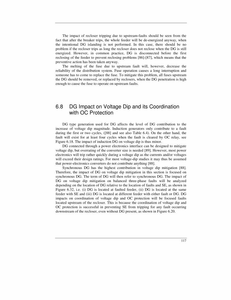
117
The impact of recloser tripping due to upstream-faults should be seen from the fact that after the breaker trips, the whole feeder will be de-energized anyway, when the intentional DG islanding is not performed. In this case, there should be no problem if the recloser trips as long the recloser does not reclose when the DG is still energized. However, in common practice, DG is disconnected before the first reclosing of the feeder to prevent reclosing problems [86]-[87], which means that the preventive action has been taken anyway. The melting of the fuse due to upstream fault will, however, decrease the reliability of the distribution system. Fuse operation causes a long interruption and someone has to come to replace the fuse. To mitigate this problem, all fuses upstream the DG should be removed, or replaced by reclosers, when the DG penetration is high enough to cause the fuse to operate on upstream faults.
6.8 DG Impact on Voltage Dip and its Coordination with OC Protection
DG type generation used for DG affects the level of DG contribution to the
increase of voltage dip magnitude. Induction generators only contribute to a fault during the first or two cycles, ([88] and see also Table 6.4). On the other hand, the fault will exist for at least four cycles when the fault is cleared by OC relay, see Figure 6.18. The impact of induction DG on voltage dip is thus minor.
DG connected through a power electronics interface can be designed to mitigate voltage dip, but overrating of the converter size is needed [89]. However, most power electronics will trip rather quickly during a voltage dip as the currents and/or voltages will exceed their design ratings. For most voltage-dip studies it may thus be assumed that power-electronics converters do not contribute anything [88].
Synchronous DG has the highest contribution in voltage dip mitigation [88]. Therefore, the impact of DG on voltage dip mitigation in this section is focused on synchronous DG. The term of DG will then refer to synchronous DG. The impact of DG on voltage dip mitigation on balanced three-phase faults will be analyzed depending on the location of DG relative to the location of faults and SE, as shown in Figure 6.32, i.e. (i) DG is located at faulted feeder, (ii) DG is located at the same feeder with SE and (iii) DG is located at different feeder with either fault or DG. DG impacts on coordination of voltage dip and OC protection will be focused faults located upstream of the recloser. This is because the coordination of voltage dip and OC protection is successful in preventing SE from tripping for any fault occurring downstream of the recloser, even without DG present, as shown in Figure 6.20.

Chapter 6: Voltage Dip and Overcurrent Protection in the Presence of DG
118
Dy
SE
Feeder-1
Feeder-2
IF
Feeder-3
DG
DG
DG(i)
(ii)
(iii)
Grid
Dy
SE
Feeder-1
Feeder-2
IF
Feeder-3
DGDG
DGDG
DGDG(i)
(ii)
(iii)
Grid
Z1,DG-F
Z1,GR
Z1,SB-DG
Z1,DG
IF,RL
IF
Z1,S-F
Z1,SB-DG
IF,GR
IFIF,DG
IF,RL
IF,DGZ1,GR
UPCC
1pu
+
1pu
+
Z1,DG
1pu+
1pu+
UPCC
Z1,S-F
Z1,SB-DG
IF,GR
IF,RL
IF,DGZ1,GR
Z1,DG
+1pu
+
UPCC
UPCC
IF,RL
1pu
Z1,DG-F
Z1,GR
Z1,SB-DG
Z1,DG
IF,RL
IF
Z1,S-F
Z1,SB-DG
IF,GR
IFIF,DG
IF,RL
IF,DGZ1,GR
UPCC
1pu
+
1pu
+
Z1,DG
1pu+
1pu+
UPCC
Z1,S-F
Z1,SB-DG
IF,GR
IF,RL
IF,DGZ1,GR
Z1,DG
+1pu
+
UPCC
UPCC
IF,RL
1pu
Z1,SB-F
Z1,SB-F
Z1,SSZ1,SS Z1,SS
++
(i) (ii) (iii)
Figure 6.32. Simple networks for the analysis of the DG contribution on voltage dip mitigation and its equivalent diagram.
Figure 6.33 shows the voltage dip sensed by the SE on three-phase faults when a 15 MVA DG is connected at different locations on feeders in Figure 6.8. The figure shows that, as previously mentioned, the DG will contribute to the increase of voltage dip magnitude; where the level of increase varies depending on DG location.
However, the support (from DG) in increasing the voltage dip magnitude may not be enough to mitigate the voltage dip problem, i.e. to prevent the SE from tripping. For example, Figure 6.34 shows the coordination of voltage dip and overcurrent protection on three-phase faults when the DG is connected at feeder-3. It is shown that the high penetration of DG on feeder-3 – as previously mentioned, 15 MVA DG power generates more than twice the total load – can not prevent the SE from tripping, because the clearing time performed by the relay and breaker is longer than the SE critical clearing time. Note that, as previously explained, with DG connection at either feeder-2 or feeder-3, the setting of IOC relay needs decreasing. The fault clearing time presented in the figure has already adopted the required instantaneous relay setting as specified in Table 6.5.
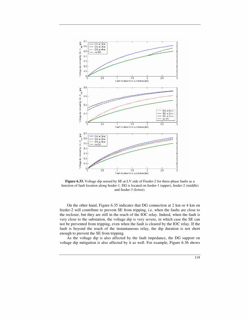
119
Figure 6.33. Voltage dip sensed by SE at LV side of Feeder-2 for three-phase faults as a
function of fault location along feeder-1. DG is located on feeder-1 (upper), feeder-2 (middle) and feeder-3 (lower).
On the other hand, Figure 6.35 indicates that DG connection at 2 km or 4 km on feeder-2 will contribute to prevent SE from tripping, i.e. when the faults are close to the recloser, but they are still in the reach of the IOC relay. Indeed, when the fault is very close to the substation, the voltage dip is very severe, in which case the SE can not be prevented from tripping, even when the fault is cleared by the IOC relay. If the fault is beyond the reach of the instantaneous relay, the dip duration is not short enough to prevent the SE from tripping. As the voltage dip is also affected by the fault impedance, the DG support on voltage dip mitigation is also affected by it as well. For example, Figure 6.36 shows
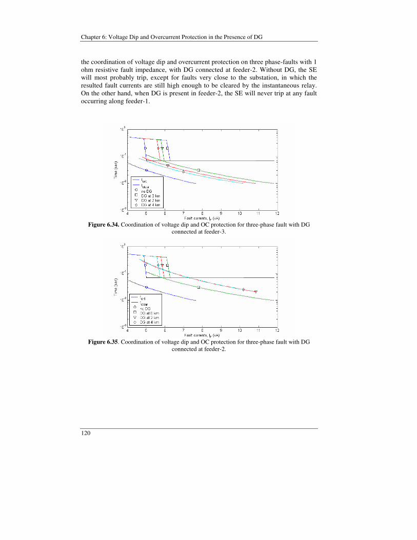
Chapter 6: Voltage Dip and Overcurrent Protection in the Presence of DG
120
the coordination of voltage dip and overcurrent protection on three phase-faults with 1 ohm resistive fault impedance, with DG connected at feeder-2. Without DG, the SE will most probably trip, except for faults very close to the substation, in which the resulted fault currents are still high enough to be cleared by the instantaneous relay. On the other hand, when DG is present in feeder-2, the SE will never trip at any fault occurring along feeder-1.
Figure 6.34. Coordination of voltage dip and OC protection for three-phase fault with DG
connected at feeder-3.
Figure 6.35. Coordination of voltage dip and OC protection for three-phase fault with DG
connected at feeder-2.
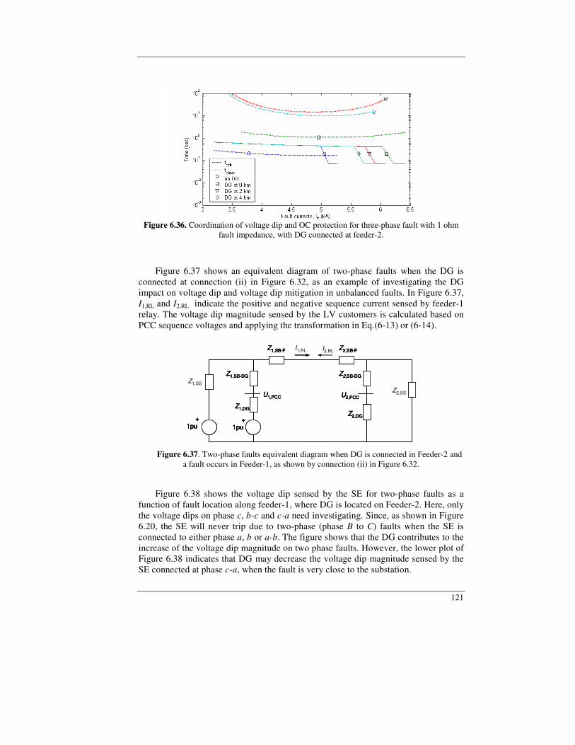
121
Figure 6.36. Coordination of voltage dip and OC protection for three-phase fault with 1 ohm
fault impedance, with DG connected at feeder-2.
Figure 6.37 shows an equivalent diagram of two-phase faults when the DG is connected at connection (ii) in Figure 6.32, as an example of investigating the DG impact on voltage dip and voltage dip mitigation in unbalanced faults. In Figure 6.37, I1,RL and I2,RL indicate the positive and negative sequence current sensed by feeder-1 relay. The voltage dip magnitude sensed by the LV customers is calculated based on PCC sequence voltages and applying the transformation in Eq.(6-13) or (6-14).
Z1,SB-F
Z1,SB-DG
IF1,RL
IF1,DGZ1,GR
Z1,DG
1pu+
1pu+
U1,PCC
Z2,SB-FIF2,RL
Z2,SB-DG IF2,DG
Z2,DG
Z2,GRU2,PCC
Z1,SB-F
Z1,SB-DG
IF1,RL
IF1,DGZ1,GR
Z1,DG
1pu+
1pu+
U1,PCC
Z2,SB-FIF2,RL
Z2,SB-DG IF2,DG
Z2,DG
Z2,GRU2,PCC
Z1,SS
Z2,SS
I1,RL I2,RLZ1,SB-F
Z1,SB-DG
IF1,RL
IF1,DGZ1,GR
Z1,DG
1pu+
1pu+
U1,PCC
Z2,SB-FIF2,RL
Z2,SB-DG IF2,DG
Z2,DG
Z2,GRU2,PCC
Z1,SB-F
Z1,SB-DG
IF1,RL
IF1,DGZ1,GR
Z1,DG
1pu+
1pu+
U1,PCC
Z2,SB-FIF2,RL
Z2,SB-DG IF2,DG
Z2,DG
Z2,GRU2,PCC
Z1,SS
Z2,SS
I1,RLI1,RL I2,RL
Figure 6.37. Two-phase faults equivalent diagram when DG is connected in Feeder-2 and
a fault occurs in Feeder-1, as shown by connection (ii) in Figure 6.32.
Figure 6.38 shows the voltage dip sensed by the SE for two-phase faults as a function of fault location along feeder-1, where DG is located on Feeder-2. Here, only the voltage dips on phase c, b-c and c-a need investigating. Since, as shown in Figure 6.20, the SE will never trip due to two-phase (phase B to C) faults when the SE is connected to either phase a, b or a-b. The figure shows that the DG contributes to the increase of the voltage dip magnitude on two phase faults. However, the lower plot of Figure 6.38 indicates that DG may decrease the voltage dip magnitude sensed by the SE connected at phase c-a, when the fault is very close to the substation.

Chapter 6: Voltage Dip and Overcurrent Protection in the Presence of DG
122
Figure 6.38. Voltage dip sensed by SE at LV side of Feeder-2 on two-phase faults as a function
of fault location along feeder-1 with DG is located on Feeder-2.
Figure 6.39 shows the coordination of voltage dip and overcurrent protection. Comparing the voltage dip in phase c in the upper plot of Figure 6.38 with a three-phase fault caused dip in Figure 6.33 (the middle plot where the DG is connected at feeder-2, too); it can be seen that both voltage dip magnitudes are the same. However, the three-phase fault current is 2/3 times of two-phase fault current, see Figure 6.10, therefore, the voltage dip duration for two-phase faults will be longer. This means that the voltage dip mitigation for two-phase faults, for these two particular cases, can be less successful than the mitigation for three phase faults (compare the upper plot of Figure 6.39 and Figure 6.35).
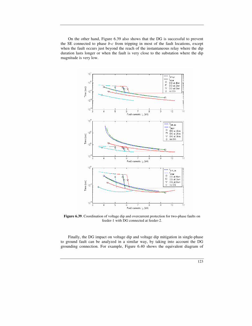
123
On the other hand, Figure 6.39 also shows that the DG is successful to prevent the SE connected to phase b-c from tripping in most of the fault locations, except when the fault occurs just beyond the reach of the instantaneous relay where the dip duration lasts longer or when the fault is very close to the substation where the dip magnitude is very low.
Figure 6.39. Coordination of voltage dip and overcurrent protection for two-phase faults on
feeder-1 with DG connected at feeder-2.
Finally, the DG impact on voltage dip and voltage dip mitigation in single-phase
to ground fault can be analyzed in a similar way, by taking into account the DG grounding connection. For example, Figure 6.40 shows the equivalent diagram of
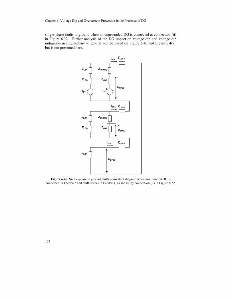
Chapter 6: Voltage Dip and Overcurrent Protection in the Presence of DG
124
single-phase faults to ground when an ungrounded DG is connected at connection (ii) in Figure 6.32. Further analysis of the DG impact on voltage dip and voltage dip mitigation in single-phase to ground will be based on Figure 6.40 and Figure 6.4(a), but is not presented here.
Z1,TX
+1pu
Z1,SB-F
Z1,GR
Z1,SB-DG
+1pu
Z1,DG
Z2,TX
Z2,SB-F
Z2,GR
Z2,SB-DG
Z2,DG
Z0,TX
Z0,SB-F
I1,RL
I2,RL
I0,RL
+
U1,PCC
+
U2,PCC
+
U0,PCC
Z1,TX
+1pu
Z1,SB-F
Z1,GR
Z1,SB-DG
+1pu
Z1,DG
Z2,TX
Z2,SB-F
Z2,GR
Z2,SB-DG
Z2,DG
Z0,TX
Z0,SB-F
I1,RL
I2,RL
I0,RL
+
U1,PCC
+
U2,PCC
+
U0,PCC
Figure 6.40. Single-phase to ground faults equivalent diagram when ungrounded DG is
connected in Feeder-2 and fault occurs in Feeder-1, as shown by connection (ii) in Figure 6.32.

125
6.9 Conclusions
In this chapter, the impact of DG on voltage dip and overcurrent protection has been investigated. The voltage dip was coordinated with overcurrent protection, and the result was compared to the voltage dip immunity of SE to investigate the impact of DG on voltage dip mitigation, i.e. preventing tripping of SE due to a voltage dip.
It has been shown that the most significant impact on short circuit and voltage dip is given by DG using synchronous generator. Therefore, detailed investigation was focused on DG using synchronous generator. It has been shown that short circuit currents will increase with the presence of DG, but, depending on where the DG is located, the DG can either increase or decrease short circuit currents sensed by PDs.
The increase or decrease of short circuit currents sensed by PDs may lead to protection problems, such as mal-coordination between an IOC relay and downstream recloser/fuse, a TOC relay does not sense high impedance faults, mal-coordination between a recloser and fuse and an IOC relay operating due to faults on adjacent feeders. Appropriate corrective actions are required to mitigate these problems, to ensure that OC protection coordination can still be held with the presence of DG.
It has been shown that DG always increases the voltage dip magnitude, i.e. the residual voltage during the dip, either balanced or unbalance voltage dip. However, DG can either lengthen or shorten voltage dip duration, which depends on whether the PD senses the decrease or the increase short circuit current. Finally, it has been shown that though DG may increase the voltage dip magnitude significantly, however sometimes the increase is not enough to prevent SE from tripping.

Chapter 6: Voltage Dip and Overcurrent Protection in the Presence of DG
126
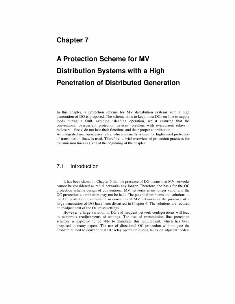
Chapter 7
A Protection Scheme for MV
Distribution Systems with a High
Penetration of Distributed Generation
In this chapter, a protection scheme for MV distribution systems with a high penetration of DG is proposed. The scheme aims to keep most DGs on-line to supply loads during a fault, avoiding islanding operation, whilst ensuring that the conventional overcurrent protection devices (breakers with overcurrent relays – reclosers – fuses) do not lose their functions and their proper coordination. An integrated microprocessor relay, which normally is used for high-speed protection of transmission lines, is used. Therefore, a brief overview of protection practices for transmission lines is given at the beginning of the chapter.
7.1 Introduction
It has been shown in Chapter 6 that the presence of DG means that MV networks
cannot be considered as radial networks any longer. Therefore, the basis for the OC protection scheme design of conventional MV networks is no longer valid, and the OC protection coordination may not be held. The potential problems and solutions to the OC protection coordination in conventional MV networks in the presence of a large penetration of DG have been discussed in Chapter 6. The solutions are focused on readjustment of the OC relay settings.
However, a large variation in DG and frequent network configurations will lead to numerous readjustments of settings. The use of transmission line protection schemes is expected to be able to minimize this requirement, which has been proposed in many papers. The use of directional OC protection will mitigate the problem related to conventional OC relay operation during faults on adjacent feeders
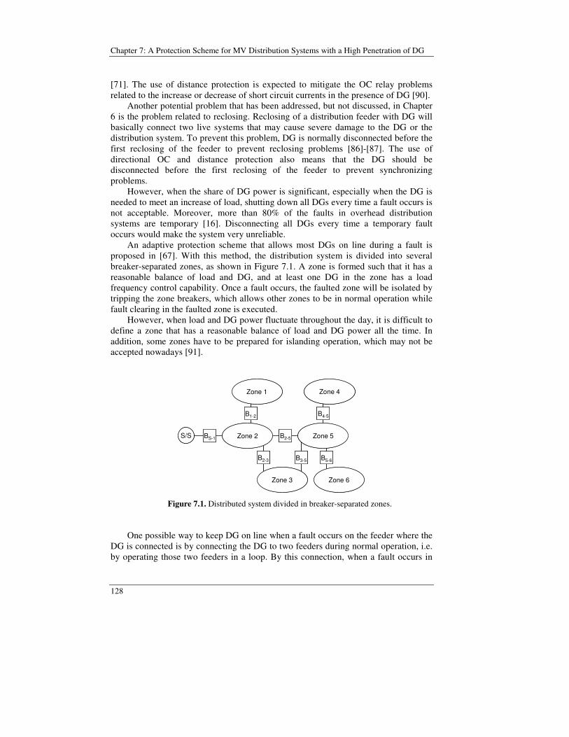
Chapter 7: A Protection Scheme for MV Distribution Systems with a High Penetration of DG
128
[71]. The use of distance protection is expected to mitigate the OC relay problems related to the increase or decrease of short circuit currents in the presence of DG [90]. Another potential problem that has been addressed, but not discussed, in Chapter 6 is the problem related to reclosing. Reclosing of a distribution feeder with DG will basically connect two live systems that may cause severe damage to the DG or the distribution system. To prevent this problem, DG is normally disconnected before the first reclosing of the feeder to prevent reclosing problems [86]-[87]. The use of directional OC and distance protection also means that the DG should be disconnected before the first reclosing of the feeder to prevent synchronizing problems. However, when the share of DG power is significant, especially when the DG is needed to meet an increase of load, shutting down all DGs every time a fault occurs is not acceptable. Moreover, more than 80% of the faults in overhead distribution systems are temporary [16]. Disconnecting all DGs every time a temporary fault occurs would make the system very unreliable. An adaptive protection scheme that allows most DGs on line during a fault is proposed in [67]. With this method, the distribution system is divided into several breaker-separated zones, as shown in Figure 7.1. A zone is formed such that it has a reasonable balance of load and DG, and at least one DG in the zone has a load frequency control capability. Once a fault occurs, the faulted zone will be isolated by tripping the zone breakers, which allows other zones to be in normal operation while fault clearing in the faulted zone is executed. However, when load and DG power fluctuate throughout the day, it is difficult to define a zone that has a reasonable balance of load and DG power all the time. In addition, some zones have to be prepared for islanding operation, which may not be accepted nowadays [91].
B5-6
S/S Zone 2BS-1
Zone 1
B1-2
Zone 5B2-5
Zone 3
B2-3 B3-5
Zone 4
B4-5
Zone 6
B5-6
S/S Zone 2BS-1
Zone 1
B1-2
Zone 5B2-5
Zone 3
B2-3 B3-5
Zone 4
B4-5
Zone 6
Figure 7.1. Distributed system divided in breaker-separated zones.
One possible way to keep DG on line when a fault occurs on the feeder where the DG is connected is by connecting the DG to two feeders during normal operation, i.e. by operating those two feeders in a loop. By this connection, when a fault occurs in

129
one of the two feeders, the DG can keep running to supply the load through its connection to the un-faulted feeder. Operation of distribution systems as a closed-loop or a mesh have been proposed in many papers. Meshed operation is intended to increase DG integration limit as in [62], which has also been discussed in Chapter 6. However, it is observed in [62] that the protection issue with meshed distribution networks is something that needs to be solved and there is a lack of studies on protection coordination in non radial networks with DG.
Protection coordination in a closed-loop distribution network with DG is presented in [92], by closing the normally open switch between two feeders, and exchange the switch with a high-speed disconnector switch. When a fault occurs on either of two feeders; firstly the high-speed switch will open, and then the conventional OC protection will trip the faulty radial feeder. With this scheme, however, the DG still has to be disconnected from the feeder at every time fault occurs. This chapter discusses a proposed protection scheme, keeping the DGs on line during the fault without islanding operation, whilst ensuring that the conventional OC PDs (breakers with OC relays – reclosers – fuses) do not lose their functions and their proper coordination. With this scheme, the distribution system will be operated in loops. The proposed scheme is intended for a distribution network with a high penetration of DG.
7.2 Protection Practices in Transmission Lines
7.2.1 Directional OC Protection
OC protection has been discussed in Chapter 6. This type of protection is widely used in a radial distribution system, because of its simplicity and cost effectiveness. However, in a system where the power flow direction is not radial, it may be impossible to set the OC protection relays that provide a selective protection system.
For example, see relay 2 and relay 3 in Figure 7.2. Relay 2 is intended to protect line-1, and relay 3 is intended to protect line-2. When OC relays are used, the relays cannot differentiate whether the fault is on line-1 or line-2, because the OC relay is not supplemented with directional elements. Therefore, both relay 2 and relay 3 will see the fault, whether it is on line-1 and line-2.
Assume that OC relays are used to protect line-1 and line-2. In order to protect line-1, relay 2 has to have a lower setting than relay 3, otherwise HV/MV substation will be disconnected from the system when there is a fault on line-1. On the other hand, relay 3 must have a lower setting than relay 2 to protect line-2, which is contradictory to the previous requirement.
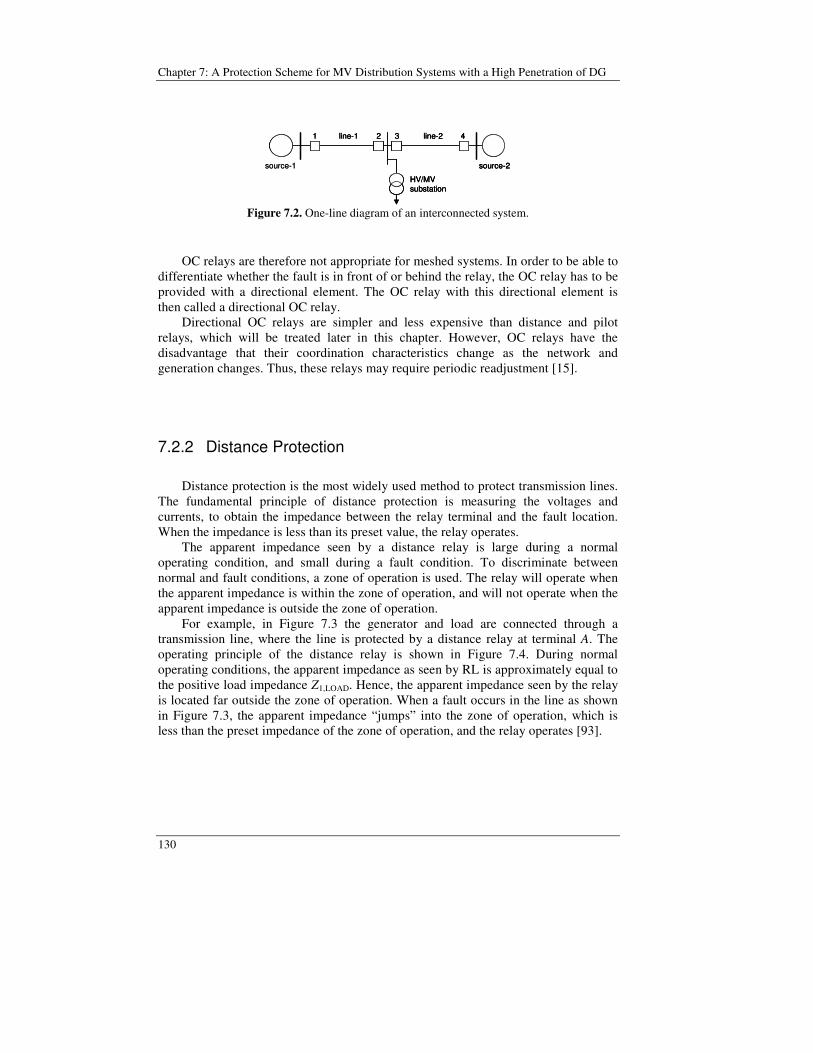
Chapter 7: A Protection Scheme for MV Distribution Systems with a High Penetration of DG
130
source-1
line-1
HV/MVsubstation
21
source-2
43 line-2
source-1
line-1
HV/MVsubstation
21
source-2
43 line-2line-1
HV/MVsubstation
21
source-2
43 line-2
Figure 7.2. One-line diagram of an interconnected system.
OC relays are therefore not appropriate for meshed systems. In order to be able to differentiate whether the fault is in front of or behind the relay, the OC relay has to be provided with a directional element. The OC relay with this directional element is then called a directional OC relay.
Directional OC relays are simpler and less expensive than distance and pilot relays, which will be treated later in this chapter. However, OC relays have the disadvantage that their coordination characteristics change as the network and generation changes. Thus, these relays may require periodic readjustment [15].
7.2.2 Distance Protection
Distance protection is the most widely used method to protect transmission lines. The fundamental principle of distance protection is measuring the voltages and currents, to obtain the impedance between the relay terminal and the fault location. When the impedance is less than its preset value, the relay operates.
The apparent impedance seen by a distance relay is large during a normal operating condition, and small during a fault condition. To discriminate between normal and fault conditions, a zone of operation is used. The relay will operate when the apparent impedance is within the zone of operation, and will not operate when the apparent impedance is outside the zone of operation.
For example, in Figure 7.3 the generator and load are connected through a transmission line, where the line is protected by a distance relay at terminal A. The operating principle of the distance relay is shown in Figure 7.4. During normal operating conditions, the apparent impedance as seen by RL is approximately equal to the positive load impedance Z1,LOAD. Hence, the apparent impedance seen by the relay is located far outside the zone of operation. When a fault occurs in the line as shown in Figure 7.3, the apparent impedance “jumps” into the zone of operation, which is less than the preset impedance of the zone of operation, and the relay operates [93].
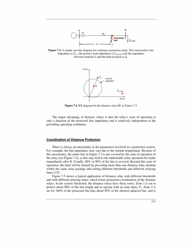
131
A B
Z1,L
ZF
Three-phasefault Z1,LOAD
A B
Z1,L
ZF
Three-phasefault Z1,LOAD
RL
Figure 7.3. A simple one-line diagram for a distance protection study. The total positive line
impedance is Z1,L, the positive load impedance is Z1,LOAD and the impedance between terminal A and the fault location is ZF.
X ()
ZF
R ()
Z1,L zone of operation
Z1,LOAD
Figure 7.4. RX diagram for the distance relay RL in Figure 7.3.
The major advantage of distance relays is that the relay’s zone of operation is only a function of the protected line impedance and is relatively independent of the prevailing operating conditions. Coordination of Distance Protection There is always an uncertainty in the parameters involved in a protection system. For example, the line impedance may vary due to the outside temperature. Because of this uncertainty, the entire line in Figure 7.3 is not covered by the zone of operation of the relay (see Figure 7.4), as this may lead to the undesirable relay operation for faults immediately after B. Usually, 80% or 90% of the line is covered. Beyond this zone of operation, the fault will be cleared by providing more than one distance relay element within the same relay package and setting different thresholds and different relaying times [15]. Figure 7.5 shows a typical application of distance relay with different thresholds and with different relaying times, which forms protection coordination of the distance relays. In the system illustrated, the distance relays have three zones. Zone 1 is set to protect about 90% of the line length and to operate with no time delay T1. Zone 2 is set for 100% of the protected line plus about 50% of the shortest adjacent line, and is
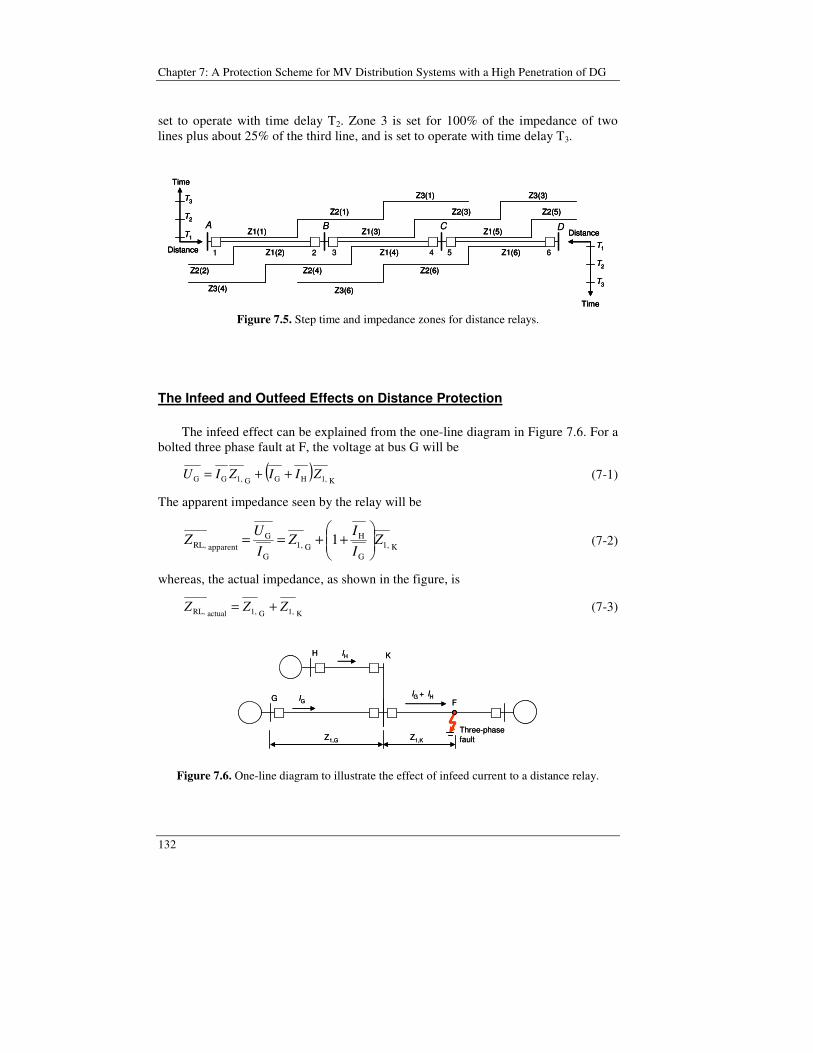
Chapter 7: A Protection Scheme for MV Distribution Systems with a High Penetration of DG
132
set to operate with time delay T2. Zone 3 is set for 100% of the impedance of two lines plus about 25% of the third line, and is set to operate with time delay T3.
Z1(1) Z1(3) Z1(5)
Z2(1) Z2(3) Z2(5)
Z3(1) Z3(3)
Distance
Time
T1
T2
T3
Z3(4) Z3(6)
Z1(2) Z1(4) Z1(6)
Z2(2) Z2(4) Z2(6)
Distance
Time
T3
T2
T1
A B C D
1 2 3 4 5 6
Z1(1) Z1(3) Z1(5)
Z2(1) Z2(3) Z2(5)
Z3(1) Z3(3)
Distance
Time
T1
T2
T3
Z3(4) Z3(6)
Z1(2) Z1(4) Z1(6)
Z2(2) Z2(4) Z2(6)
Distance
Time
T3
T2
T1
Z1(1) Z1(3) Z1(5)
Z2(1) Z2(3) Z2(5)
Z3(1) Z3(3)
Distance
Time
T1
T2
T3
Z3(4) Z3(6)
Z1(2) Z1(4) Z1(6)
Z2(2) Z2(4) Z2(6)
Distance
Time
T3
T2
T1
A B C D
1 2 3 4 5 6
Figure 7.5. Step time and impedance zones for distance relays.
The Infeed and Outfeed Effects on Distance Protection
The infeed effect can be explained from the one-line diagram in Figure 7.6. For a bolted three phase fault at F, the voltage at bus G will be
( )K,1HGG1,GG ZIIZIU ++= (7-1)
The apparent impedance seen by the relay will be
K1,G
HG1,
G
GapparentRL, 1 Z
II
ZI
UZ
++== (7-2)
whereas, the actual impedance, as shown in the figure, is
K1,G1,actualRL, ZZZ += (7-3)
G
K
IG
IH
IG + IH
Z1,G
F
Three-phase fault
H
Z1,K
G
K
IG
IH
IG + IH
Z1,G
F
Three-phase fault
H
Z1,K
Figure 7.6. One-line diagram to illustrate the effect of infeed current to a distance relay.

133
If IH is 0 (no infeed), ZRL,apparent is equal to ZRL,actual. As the infeed increases in proportion to IG, ZRL,apparent increases by the factor (IH/IG)Z1,K. Since this impedance, as ‘‘measured’’ by the distance relay, is larger than the actual value, the reach of the relay decreases. That is, the relay protects a smaller portion of the line as the infeed increases.
The outfeed effect can be explained from the one-line diagram in Figure 7.7. For simplicity, assume that Z1,H = Z1,J + Z1,M. Zone-1 of the distance relay at G is set as
( )J1,G1,settingRL, 9.0 ZZZ += (7-4)
The three-phase fault current sensed by the relay will be
H1,G1,SS1,JHRL 5.0
1ZZZ
III++
=+= (7-5)
The voltage sensed by the relay due to this fault will be
H1,G1,SS1,
H1,G1,RL 5.0
5.0
ZZZ
ZZU
+++
= (7-6)
The apparent impedance seen by the relay will then be
H1,G1,RL
RLapparentRL, 5.0 ZZ
IU
Z +== (7-7)
The relay at G will trip for a three-phase fault at J when
settingRL,apparentRL, ZZ <
or, from Eqs. (7-4) and (7-7), it will occur when
G1,
J1,
H1, 2.08.1 ZZ
Z−< (7-8)
For example, the relay at G will operate due to a three-phase fault at bus H when the length of the line between stations G and K, K and J, and K and H is 2, 6 and 8 km, respectively, the impedance per km being equal for all lines.
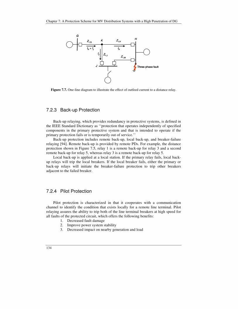
Chapter 7: A Protection Scheme for MV Distribution Systems with a High Penetration of DG
134
G
Three-phase fault
H
J
K
IH
IJ
IH + IJ
Z1,G
Z1,J
Z1,H
Z1,M
G
Three-phase fault
H
J
K
IH
IJ
IH + IJ
Z1,G
Z1,J
Z1,H
Z1,M
Figure 7.7. One-line diagram to illustrate the effect of outfeed current to a distance relay.
7.2.3 Back-up Protection
Back-up relaying, which provides redundancy in protective systems, is defined in the IEEE Standard Dictionary as ‘‘protection that operates independently of specified components in the primary protective system and that is intended to operate if the primary protection fails or is temporarily out of service.’’
Back-up protection includes remote back-up, local back-up, and breaker-failure relaying [94]. Remote back-up is provided by remote PDs. For example, the distance protection shown in Figure 7.5, relay 1 is a remote back-up for relay 3 and a second remote back-up for relay 5, whereas relay 3 is a remote back-up for relay 5.
Local back-up is applied at a local station. If the primary relay fails, local back-up relays will trip the local breakers. If the local breaker fails, either the primary or back-up relays will initiate the breaker-failure protection to trip other breakers adjacent to the failed breaker.
7.2.4 Pilot Protection
Pilot protection is characterized in that it cooperates with a communication channel to identify the condition that exists locally for a remote line terminal. Pilot relaying assures the ability to trip both of the line terminal breakers at high speed for all faults of the protected circuit, which offers the following benefits:
1. Decreased fault damage 2. Improve power system stability 3. Decreased impact on nearby generation and load

135
This protection is applicable at all voltages. In actual practice, it is usually applied to short lines at all voltages and to most lines at about 69 – 115 kV and higher. According to [16], the major pilot systems in use can be identified more specifically in the following classification:
A. Directional comparison systems 1. Blocking Scheme 2. Unblocking Scheme 3. Permissive Overreaching Transfer Trip 4. Underreaching Transfer Trip
a. Permissive Underreaching Transfer Trip b. Direct Underreaching Transfer Trip
B. Phase comparison systems 1. “Pilot Wire” 2. Single-phase Comparison: blocking 3. Dual-phase Comparison: unblocking 4. Dual-phase Comparison: transfer trip 5. Segregated Phase Comparison
C. Directional wave comparison
The directional comparison uses the fundamental concept that directional units at both line terminals must agree that the direction to a fault is toward the protected line, then tripping of circuit breaker at both terminals is initiated.
The phase comparison type compares the phase angle relation between single-phase voltages at two terminal-ends with the aid of the communication channel. During normal operating condition, the phase angle difference between currents at both terminals is small, whereas when an internal fault occurs, the phase angle difference shifts approximately 1800 and the protection scheme operates to trip the circuit breaker at both terminals.
The directional wave comparison uses the concept that an electrical disturbance generates traveling waves that spread outward from the disturbed area, traveling down the line in opposite directions. If the fault is external, the wave direction will be in at one terminal and out at the other. Thus, comparing the wave direction at the terminals by a microwave or power-line carrier channel provides an indication of a fault and its location. This provides ultra-high speed distance protection for lines of 350 kV and more [16].
This thesis will only discuss Permissive Overreaching Transfer Trip (POTT). Other pilot schemes can be read in [16] and [95]. Further, communication technologies required for the scheme are beyond the scope of this thesis.
POTT depends on overreaching phase and ground relays to recognize the presence of a fault on the protected circuit and to initiate the transmission of a trip request to the remote terminal. Normally a directional phase distance relay is used for phase protection and either directional ground distance or directional instantaneous ground OC relay are used for ground protection [16].
The basic operating principle of POTT scheme is shown in Figure 7.8. When there is an internal fault in the protected zone, both FD1 and FD2 operate to shift their
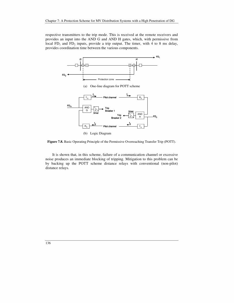
Chapter 7: A Protection Scheme for MV Distribution Systems with a High Penetration of DG
136
respective transmitters to the trip mode. This is received at the remote receivers and provides an input into the AND G and AND H gates, which, with permissive from local FD1 and FD2 inputs, provide a trip output. The timer, with 4 to 8 ms delay, provides coordination time between the various components.
1 2
G HFD1
FD2
Protection zone
1 2
G HFD1
FD2
Protection zone (a) One-line diagram for POTT scheme
Pilot channelf1
FD2
ANDH
Trip Breaker 2
o
timer
ANDG
Trip Breaker 1
RH
FDF1
f1TG
otimer
RG Pilot channelf2
TH
f2
Pilot channelf1
FD2
ANDH
Trip Breaker 2
oo
timer
ANDG
Trip Breaker 1
RH
FDF1
f1f1TG
ootimer
RG Pilot channelf2
TH
f2
(b) Logic Diagram
Figure 7.8. Basic Operating Principle of the Permissive Overreaching Transfer Trip (POTT).
It is shown that, in this scheme, failure of a communication channel or excessive noise produces an immediate blocking of tripping. Mitigation to this problem can be by backing up the POTT scheme distance relays with conventional (non-pilot) distance relays.
137
7.3 The Use of HV Transmission Lines Protection Schemes to Protect MV Distribution Lines with DG
With the presence of DG, the distribution systems will look like transmission
systems, and they can not be considered as radial systems any longer. Further, the short circuit levels in the distribution systems will vary significantly according to variations in DG configuration in the system. Therefore, the use of transmission system protection schemes is expected to be able to mitigate the problems that are faced by conventional distribution system protection schemes, i.e. protection schemes based on OC PDs without directional discrimination.
The use of directional OC relays will obviously prevent a relay from tripping due to faults on adjacent feeders, as can be concluded from Section 7.2.1. The drawback of the use of directional OC relay in feeders with DG is that the reach of the relay is affected by the variations of DG configuration in the system.
The use of distance protection will mitigate the variation in relay reach due to the DG. The installation of several distance relays in series in a MV feeder with DG is presented in [90]. It is illustrated that distance relays can coordinate well on different DG configurations. One should note that, when there is DG inside the protected area, the DG acts as the infeed to the fault and causes the distance relay to underreach. This is similar to what has been explained in Section 7.2.2.
Zone-1 distance relays can be applied to provide increased instantaneous protection, close to 90% instantaneous coverage of the line section, because of its independency to the variation of short circuit level. On the other hand, zone-2 and zone-3 cannot directly be used to coordinate with existing downstream OC PDs (reclosers and fuses). This is because the distance relays have a constant time delay (Section 7.2.2), whereas, it has been shown in Chapter 6 that the reclosers and fuses have a varying time delay, which is inversely proportional to the fault current. However, the coordination between the distance relays and reclosers and fuses is still possible, for instance, by using inverse-time-OC relays as a timer for the zone-2 and zone-3 distance relay [16]. Or, alternatively, if the distance relay is provided with programmable time delays.

Chapter 7: A Protection Scheme for MV Distribution Systems with a High Penetration of DG
138
7.4 Proposed Protection Scheme In order to keep most DGs on line to supply loads during the fault without putting DG in islanding operation, the DG needs to be connected to two feeders that are operated in a loop by closing the normally open switch. This should not be difficult, since, as previously mentioned, MV networks are typically designed partly meshed though they are operated in open loops. When a fault occurs, the DG has to be disconnected from the faulted feeder while its connection to the un-faulted feeder has to be kept to deliver the DG power. An example of DG connection to the MV network with the proposed scheme is shown in Figure 7.9. Breaker 1 and 2 are needed to connect DG1, whereas breaker 3, 4 and 5 are needed to connect DG2. Some breakers are coordinated to form a protection coordination area, for example breaker 1 and F1 form protection coordination Area-1. Further, fuse f3 should be omitted with the connection of DG2, otherwise fuse operation will cause long interruption for the DG, or it is also possible that the fuse will melt on upstream faults and cause long interruption for faults that the fuse is not supposed to clear, as has been explained in Chapter 6.
F1
f1 f2 f3
Grid
Substation Transformer
F2
R1R2
F1
f1 f2
Substation Transformer
F2
R1 1 2
DG1
R23
4
5DG2
S
Grid
S
Area-1 Area-2
Area-3
Area-4
F1
f1 f2 f3
Grid
Substation Transformer
F2
R1R2
F1
f1 f2
Substation Transformer
F2
R1 1 2
DG1
R23
4
5DG2
S
Grid
S
F1
f1 f2 f3
Grid
Substation Transformer
F2
R1R2
F1
f1 f2
Substation Transformer
F2
R1 1 2
DG1
R23
4
5DG2
S
Grid
S
Area-1 Area-2
Area-3
Area-4
Figure 7.9. Radially operated MV system with mesh construction (left) and meshed operated system with the proposed scheme (right). “O”, “∅” and “” indicates normally open switch,
closed normally open switch and connection to other feeder, respectively.
In general, the algorithm of the proposed protection scheme is as shown in Figure 7.10. The protection scheme is divided into three tasks. The first task is to break up the loop and put the faulted feeder into radial operation. The second task is to clear the fault in the faulted section. Depending on the network configuration, the second

139
task can be already covered in the first task. The last task is to put the feeders back to meshed operation in case of a temporary fault. Each task has a different algorithm and different type or relay or numbers of breakers are involved, which depends on the MV network configuration in the protected area.
Feeder in loop?
yes
no
End
yes
1
2Clear the fault
Fault
Start
Break up the loop
no
Restore the loop
yes
Lock Out all opened breakers
Fault clearing successful?
Fault
no
3
Feeder in loop?
yes
no
End
yes
1
2Clear the fault
Fault
Start
Break up the loop
no
Restore the loop
yes
Lock Out all opened breakers
Fault clearing successful?
Fault
no
3
Figure 7.10. General algorithm of the proposed scheme.
To perform all of those tasks, a microprocessor-based high-speed line protection relay normally used for protection of transmission systems, is needed. The relay should at least have the following features: distance with pilot scheme, directional OC, synchronism-check, reclosing, breaker failure and programmable logic input/output. Such relays are available in the market, [96]-[97] for example.
7.4.1 Breaking Up the Loop
The first task is performed by coordinating two relays facing the fault on a pilot POTT scheme and corresponding breakers, with the coordination area as shown in Figure 7.9. The POTT scheme is formed by distance protection. Alternatively, ground directional IOC can also be used in the POTT scheme as back-up for the ground distance relay. As requested in a POTT scheme, all relays are set overreaching. Pilot scheme is selected because of the ability to trip the breaker at high speed for all faults of the protected circuit. Meanwhile, the POTT scheme can in principle be replaced by
Chapter 7: A Protection Scheme for MV Distribution Systems with a High Penetration of DG
140
other pilot schemes. Note, however, that in this proposed protection scheme, the pilot scheme does not necessarily trip breakers at all terminals, as will be illustrated later. Different coordination scheme will be applied for different relays, which depend on the presence of protective devices within the coordination area. For example, coordination schemes among relays in each coordination area can be explained as follows: Area-1 See Area-1 in Figure 7.9 where relay F1 and 1 should coordinate with each other. There are a recloser R1 and a fuse within this area, thus tripping both breakers should be avoided. The loop can then be broken up by POTT scheme tripping breaker 1. Breaker 1 will only be tripped after relay 1 sends a permissive signal for the remote signal that is obtained from relay F1. As previously explained, the POTT scheme may fail due to the failure of communication channel or excessive noise, which will block the trip. This requests back up from non-pilot distance protection that are set underreaching without time delay, or those relays with overreaching setting provided that a certain time delay is applied, or both of them. The non-pilot distance protection in relay 1 will operate to trip breaker 1 without any permissive. Alternatively, ground directional OC protection can also be used to work redundantly with ground distance protection, both in pilot and in non pilot schemes. There is also the possibility that breakers fail to trip. In (non-pilot) distance and OC protection coordination, the remote relays will automatically sense the fault should the local breaker not trip. But, in pilot scheme, the relay will not operate when the fault occurs outside their protective area. To mitigate this problem, the scheme is also provided with breaker failure function. With this function, relay 1 will trip breaker 2 and generator G1 when breaker 1 fails to open. The logic diagram of POTT coordination scheme in Area-1 is shown in Figure 7.11. Area-2 As can be seen from Figure 7.9, there is neither fuse nor recloser in Area-2, thus both breakers can be tripped simultaneously by the POTT scheme. As in the previous case, the POTT scheme should be backed up by a non-pilot scheme, and breaker failure protection should also be provided. When breaker F2 fails, relay F2 will trip all breakers at the substation; and when breaker 4 fails, relay 4 will trip both breaker 3 and 5. The logic diagram of POTT coordination scheme between relay 4 and F2 is shown in Figure 7.12. Area-3 and Area- 4 As there is fuse f2 within Area-3, POTT coordination scheme for this area is similar with the one in Area-1, where one breaker will be tripped by the scheme, i.e. breaker 2. When breaker 2 fails to open, relay 2 will trip breaker 1 and generator G1. Similarly, coordination scheme for Area-4 will also trip one breaker, i.e. breaker 3. However, since breaker 3 and breaker 4 are at the same bus, both relays will
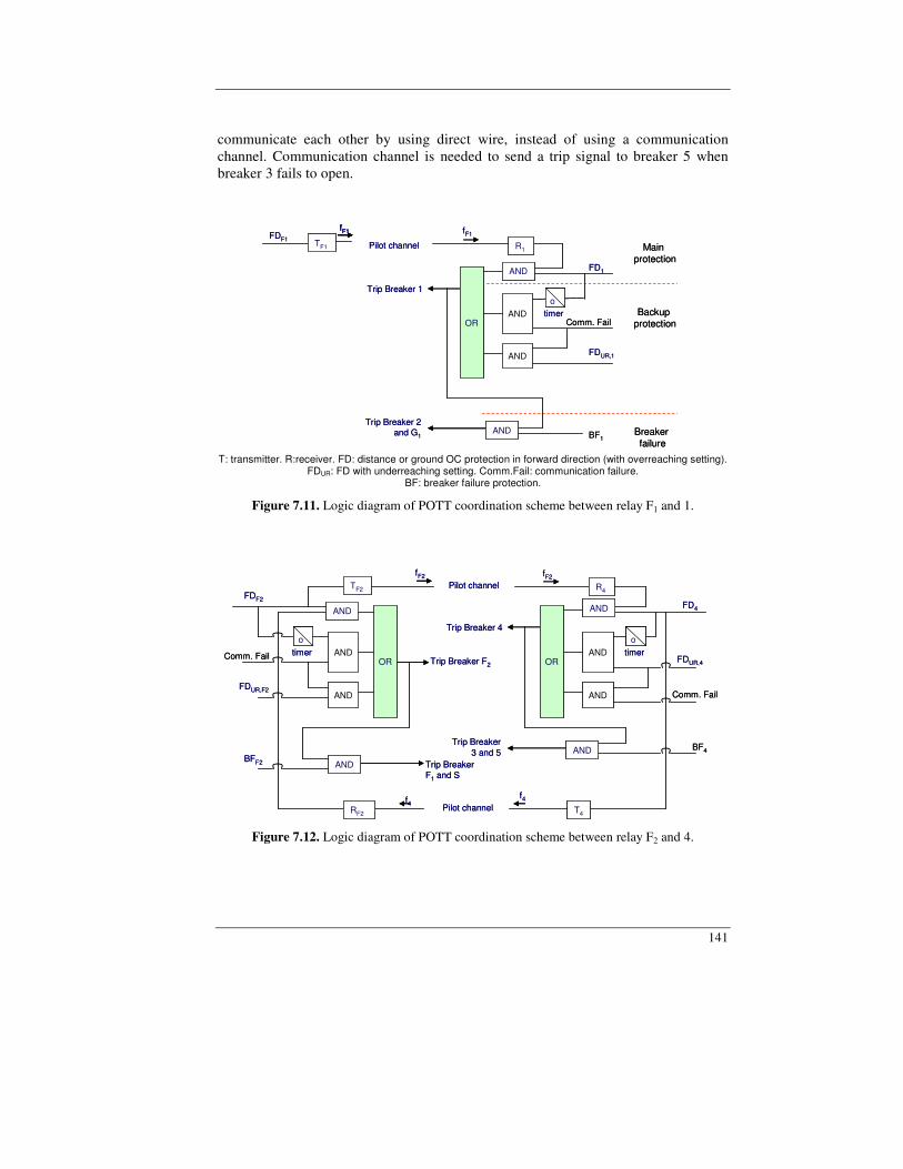
141
communicate each other by using direct wire, instead of using a communication channel. Communication channel is needed to send a trip signal to breaker 5 when breaker 3 fails to open.
Pilot channel
fF1
AND
otimer
Trip Breaker 1
Main protection
Breaker failure
Trip Breaker 2 and G1
R1
FDF1
fF1
TF1
Backup protection
BF1
FD1
Comm. FailAND
AND FDUR,1
OR
AND
Pilot channel
fF1
AND
ootimer
Trip Breaker 1
Main protection
Breaker failure
Trip Breaker 2 and G1
R1
FDF1
fF1fF1
TF1
Backup protection
BF1
FD1
Comm. FailAND
AND FDUR,1
OR
AND
T: transmitter. R:receiver. FD: distance or ground OC protection in forward direction (with overreaching setting).
FDUR: FD with underreaching setting. Comm.Fail: communication failure. BF: breaker failure protection.
Figure 7.11. Logic diagram of POTT coordination scheme between relay F1 and 1.
Pilot channelfF2
AND
otimer
Trip Breaker 4
f4Pilot channel
Trip Breaker 3 and 5
R4FDF2
fF2
RF2
f4
TF2
T4
BF4
FD4
Comm. Fail
AND
AND
FDUR,4OR
AND
AND
OR Trip Breaker F2
AND
AND
otimerComm. Fail
FDUR,F2
AND Trip Breaker F1 and S
BFF2
Pilot channelfF2
AND
ootimer
Trip Breaker 4
f4Pilot channel
Trip Breaker 3 and 5
R4FDF2
fF2
RF2
f4
TF2
T4
BF4
FD4
Comm. Fail
AND
AND
FDUR,4OR
AND
AND
OR Trip Breaker F2
AND
AND
ootimerComm. Fail
FDUR,F2
AND Trip Breaker F1 and S
BFF2
Figure 7.12. Logic diagram of POTT coordination scheme between relay F2 and 4.
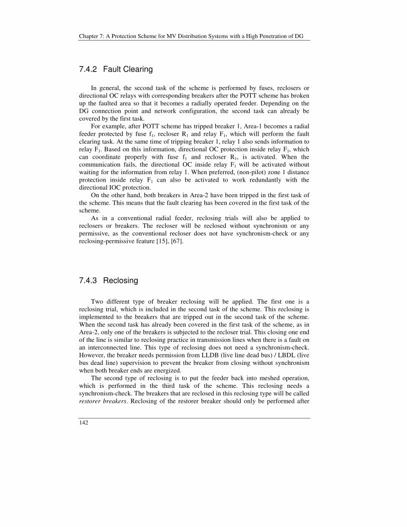
Chapter 7: A Protection Scheme for MV Distribution Systems with a High Penetration of DG
142
7.4.2 Fault Clearing In general, the second task of the scheme is performed by fuses, reclosers or directional OC relays with corresponding breakers after the POTT scheme has broken up the faulted area so that it becomes a radially operated feeder. Depending on the DG connection point and network configuration, the second task can already be covered by the first task. For example, after POTT scheme has tripped breaker 1, Area-1 becomes a radial feeder protected by fuse f1, recloser R1 and relay F1, which will perform the fault clearing task. At the same time of tripping breaker 1, relay 1 also sends information to relay F1. Based on this information, directional OC protection inside relay F1, which can coordinate properly with fuse f1 and recloser R1, is activated. When the communication fails, the directional OC inside relay F1 will be activated without waiting for the information from relay 1. When preferred, (non-pilot) zone 1 distance protection inside relay F1 can also be activated to work redundantly with the directional IOC protection. On the other hand, both breakers in Area-2 have been tripped in the first task of the scheme. This means that the fault clearing has been covered in the first task of the scheme. As in a conventional radial feeder, reclosing trials will also be applied to reclosers or breakers. The recloser will be reclosed without synchronism or any permissive, as the conventional recloser does not have synchronism-check or any reclosing-permissive feature [15], [67].
7.4.3 Reclosing
Two different type of breaker reclosing will be applied. The first one is a reclosing trial, which is included in the second task of the scheme. This reclosing is implemented to the breakers that are tripped out in the second task of the scheme. When the second task has already been covered in the first task of the scheme, as in Area-2, only one of the breakers is subjected to the recloser trial. This closing one end of the line is similar to reclosing practice in transmission lines when there is a fault on an interconnected line. This type of reclosing does not need a synchronism-check. However, the breaker needs permission from LLDB (live line dead bus) / LBDL (live bus dead line) supervision to prevent the breaker from closing without synchronism when both breaker ends are energized. The second type of reclosing is to put the feeder back into meshed operation, which is performed in the third task of the scheme. This reclosing needs a synchronism-check. The breakers that are reclosed in this reclosing type will be called restorer breakers. Reclosing of the restorer breaker should only be performed after

143
ensuring that the fault has been cleared, i.e. when one temporary fault period has elapsed and the line has been back to normal, which is recognized from the restorer breaker sensing voltage on both sides (live line live bus, LLLB). Based on the tasks explained above in Section 7.4.1 - 7.4.3, the protection algorithm for relay 1 and F1 in Area-1, for instance, can be developed as shown in Figure 7.13. The algorithm can be explained as follows: 1. The scheme is started by POTT scheme tripping breaker 1 when there is a fault in
Area-1 and breaker 1 is closed. Timer 1 (timer to restore the loop) starts. 2. When breaker 1 opens; the directional OC protection (67) scheme inside relay F1
is activated. When the fault is within F1 protected area, the fault will still be present until the delay time of the relay 67 is reached, and the relay will trip breaker F1. Otherwise, the fault is either under recloser R1 or under fuse F1 and they will trip/melt to clear the fault.
3. After a certain time delay, breaker F1 is commanded to reclose with LLDB/LBDL control.
4. If the fault is still present when the maximum number of reclosing trials is reached, the fault is considered as a permanent fault, and breaker F1 is locked out (staying open). If not, the fault is temporary, and breaker F1 will be closed.
5. Timer 1 has elapsed. If breaker 1 senses LLLB, for example when breaker F1 is closed after clearing the fault, a reclosing signal is initiated to breaker 1 and the breaker will close after the synchronism conditions are reached. If breaker 1 does not sense LLLB, for example when breaker F1 is locked out (open), the reclosing signal will not be initiated to breaker 1 and breaker 1 will be locked out.
Finally, the one-line protection diagram of the MV network in Figure 7.9 with the proposed scheme is shown in Figure 7.14. Both phase and ground protections are activated, which is not shown. Distance, directional OC and breaker failure are activated in all relays, though, as explained before, they are not activated at the same time. To reduce the number of relays required, one relay may be used to protect two lines. For example, relay 3 is used to protect Area-3 and Area-4, whereas relay 4 is used to protect Area-3 and Area-4. For this purpose, both forward and reverse directions of the distance and directional OC protection are activated. Reclosing and undervoltage supervision are activated in all relays. Meanwhile, a synchronism-check will only be activated for restorer breakers. Note that the same breaker can act as both restorer and non-restorer breaker. For example, breaker 4 will be used as restorer breaker in Area-2, and as non-restorer breaker in area-4.
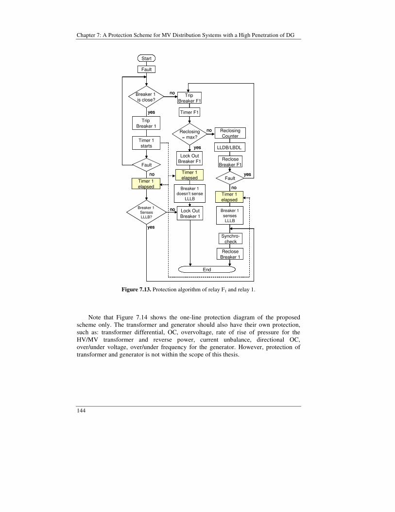
Chapter 7: A Protection Scheme for MV Distribution Systems with a High Penetration of DG
144
Start
Breaker 1 is close?
Trip Breaker 1
yes
no
Timer F1
Lock OutBreaker F1
Trip Breaker F1
Fault
Fault
RecloseBreaker F1
Timer 1starts
Reclosing= max?
yes
End
Timer 1elapsed
Synchro-check
RecloseBreaker 1
no
yes
no
Timer 1elapsed
Lock OutBreaker 1
Breaker 1doesn’t sense
LLLB
Fault
Timer 1elapsed
Breaker 1 SensesLLLB?
no
no Breaker 1sensesLLLB
yes
ReclosingCounter
LLDB/LBDL
Figure 7.13. Protection algorithm of relay F1 and relay 1.
Note that Figure 7.14 shows the one-line protection diagram of the proposed scheme only. The transformer and generator should also have their own protection, such as: transformer differential, OC, overvoltage, rate of rise of pressure for the HV/MV transformer and reverse power, current unbalance, directional OC, over/under voltage, over/under frequency for the generator. However, protection of transformer and generator is not within the scope of this thesis.
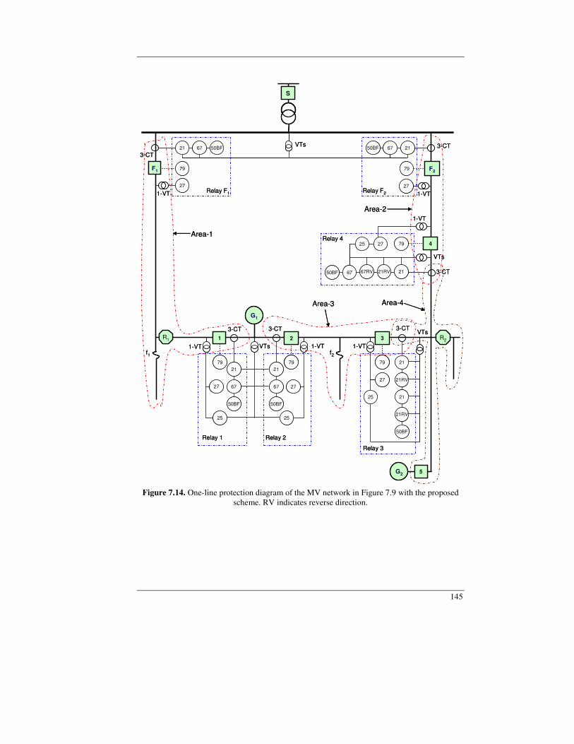
145
5
VTs
F1
3-CT21 67 50BF
79
1-VT27
G1
3-CT 3-CT
21
50BF
79
27
25
21
67
50BF
79
25
27
1-VT 1-VTVTs
3-CT
21
21RV
50BF
79
27
1-VT
VTs
3-CT21
79
50BF
F2
27
1-VT
1 2 3
G2
25
67
Relay F1 Relay F2
4
3-CT
79
21RV67RV6750BF
1-VT
25 27
21
Relay 4
67
Relay 1 Relay 2
21
21RV
Relay 3
S
VTs
R1 R2
f1 f2
Area-1
Area-2
Area-3 Area-4
5
VTs
F1
3-CT21 67 50BF
79
1-VT27
G1
3-CT 3-CT
21
50BF
79
27
25
21
67
50BF
7979
25
27
1-VT 1-VTVTs
3-CT
21
21RV
50BF
7979
27
1-VT
VTs
3-CT21
79
50BF
F2
27
1-VT
1 2 3
G2
25
67
Relay F1 Relay F2
4
3-CT
79
21RV67RV6750BF
1-VT
25 27
21
Relay 4
67
Relay 1 Relay 2
21
21RV
Relay 3
S
VTs
R1 R2
f1 f2
Area-1
Area-2
Area-3 Area-4
Figure 7.14. One-line protection diagram of the MV network in Figure 7.9 with the proposed
scheme. RV indicates reverse direction.
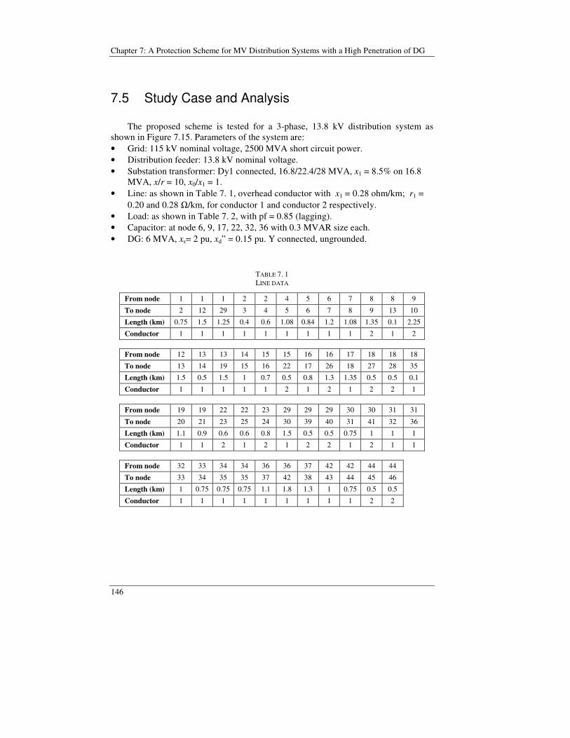
Chapter 7: A Protection Scheme for MV Distribution Systems with a High Penetration of DG
146
7.5 Study Case and Analysis The proposed scheme is tested for a 3-phase, 13.8 kV distribution system as shown in Figure 7.15. Parameters of the system are: • Grid: 115 kV nominal voltage, 2500 MVA short circuit power. • Distribution feeder: 13.8 kV nominal voltage. • Substation transformer: Dy1 connected, 16.8/22.4/28 MVA, x1 = 8.5% on 16.8
MVA, x/r = 10, x0/x1 = 1. • Line: as shown in Table 7. 1, overhead conductor with x1 = 0.28 ohm/km; r1 =
0.20 and 0.28 Ω/km, for conductor 1 and conductor 2 respectively. • Load: as shown in Table 7. 2, with pf = 0.85 (lagging). • Capacitor: at node 6, 9, 17, 22, 32, 36 with 0.3 MVAR size each. • DG: 6 MVA, xs= 2 pu, xd” = 0.15 pu. Y connected, ungrounded.
TABLE 7. 1 LINE DATA
From node 1 1 1 2 2 4 5 6 7 8 8 9
To node 2 12 29 3 4 5 6 7 8 9 13 10
Length (km) 0.75 1.5 1.25 0.4 0.6 1.08 0.84 1.2 1.08 1.35 0.1 2.25
Conductor 1 1 1 1 1 1 1 1 1 2 1 2
From node 12 13 13 14 15 15 16 16 17 18 18 18
To node 13 14 19 15 16 22 17 26 18 27 28 35
Length (km) 1.5 0.5 1.5 1 0.7 0.5 0.8 1.3 1.35 0.5 0.5 0.1
Conductor 1 1 1 1 1 2 1 2 1 2 2 1
From node 19 19 22 22 23 29 29 29 30 30 31 31
To node 20 21 23 25 24 30 39 40 31 41 32 36
Length (km) 1.1 0.9 0.6 0.6 0.8 1.5 0.5 0.5 0.75 1 1 1
Conductor 1 1 2 1 2 1 2 2 1 2 1 1 From node 32 33 34 34 36 36 37 42 42 44 44
To node 33 34 35 35 37 42 38 43 44 45 46
Length (km) 1 0.75 0.75 0.75 1.1 1.8 1.3 1 0.75 0.5 0.5
Conductor 1 1 1 1 1 1 1 1 1 2 2
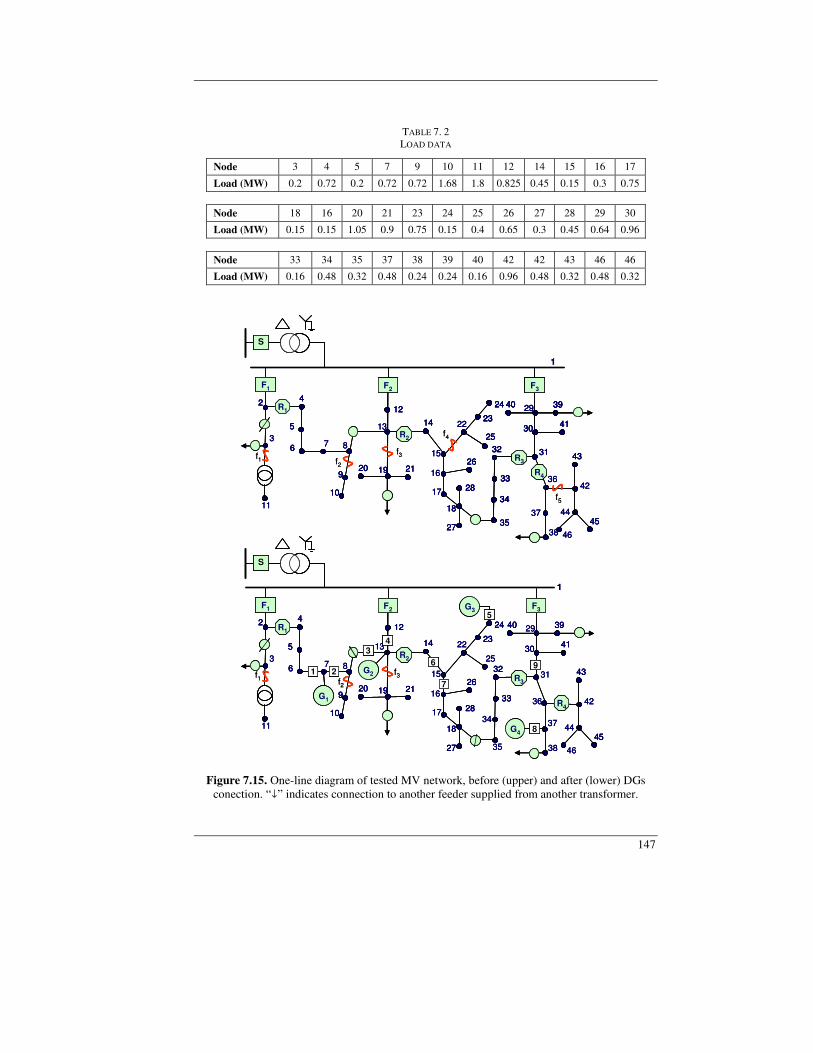
147
TABLE 7. 2 LOAD DATA
Node 3 4 5 7 9 10 11 12 14 15 16 17
Load (MW) 0.2 0.72 0.2 0.72 0.72 1.68 1.8 0.825 0.45 0.15 0.3 0.75 Node 18 16 20 21 23 24 25 26 27 28 29 30
Load (MW) 0.15 0.15 1.05 0.9 0.75 0.15 0.4 0.65 0.3 0.45 0.64 0.96 Node 33 34 35 37 38 39 40 42 42 43 46 46
Load (MW) 0.16 0.48 0.32 0.48 0.24 0.24 0.16 0.96 0.48 0.32 0.48 0.32
20
7 8
9
10
F2
12
211920
13 14
17
35
41
15
23
25
22
24
1626
1834
33
27
28
2
11
37 8
9
10
F1
R1
R2
38
37
36
4
5
6
S
1
G1
2
34
F3
32
29 3940
30
1
319
G4
G2
G3
6
5
7
8
42
46
44
43
45
R4
2
11
3
F1
R1
4
5
6
S
R3
F2
12
2119
13 14
17
15
22
1626
18
27
28
R2
F3
29 3940
3023
25
24
R331
41
38
37
36R4
42
46
44
43
45
32
35
34
33
1
f1 f2
f3
f4
f5
f3
f1 f2 20
7 8
9
10
F2
12
211920
13 14
17
35
41
15
23
25
22
24
1626
1834
33
27
28
2
11
37 8
9
10
F1
R1
R2
38
37
36
4
5
6
S
1
G1
2
34
F3
32
29 3940
30
1
319
G4
G2
G3
6
5
7
8
42
46
44
43
45
R4
2
11
3
F1
R1
4
5
6
S
R3
F2
12
2119
13 14
17
15
22
1626
18
27
28
R2
F3
29 3940
3023
25
24
R331
41
38
37
36R4
42
46
44
43
45
32
35
34
33
1
2020
7 8
99
1010
F2
1212
212119192020
13 1414
17
35
4141
15
2323
25
22
2424
162626
181834
3333
2727
2828
22
11
37 8
99
1010
F1
R1
R2
38
37
36
44
55
66
SSS
1
G1
21
G1
2
34
F3
3232
29 39394040
3030
1
319
G4
G2
G3
6
5
7
8
42
46
44
4343
4545
R4
22
11
3
F1
R1
44
55
66
SSS
R3
F2
1212
21211919
13 1414
17
15
22
162626
1818
2727
2828
R2
F3
29 3940
3023
25
24
R331
F3
29 39394040
30302323
25
2424
R331
4141
38
37
36R4
42
46
44
4343
4545
32
35
34
33
3232
35
3434
3333
1
f1 f2
f3
f4
f5
f3
f1 f2
Figure 7.15. One-line diagram of tested MV network, before (upper) and after (lower) DGs conection. “” indicates connection to another feeder supplied from another transformer.
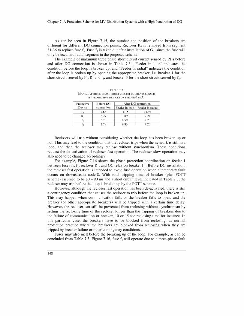
Chapter 7: A Protection Scheme for MV Distribution Systems with a High Penetration of DG
148
As can be seen in Figure 7.15, the number and position of the breakers are different for different DG connection points. Recloser R4 is removed from segment 31-36 to replace fuse f5. Fuse f4 is taken out after installation of G3, since the fuse will only be used in a radial segment in the proposed scheme. The example of maximum three phase short circuit current sensed by PDs before and after DG connection is shown in Table 7.3. “Feeder in loop” indicates the condition before the loop is broken up; and “Feeder in radial” indicates the condition after the loop is broken up by opening the appropriate breaker, i.e. breaker 1 for the short circuit sensed by F1, R1 and f1, and breaker 3 for the short circuit sensed by f2.
TABLE 7.3 MAXIMUM THREE-PHASE SHORT CIRCUIT CURRENTS SENSED
BY PROTECTIVE DEVICES ON FEEDER-1 (KA)
After DG connection Protective Device
Before DG connection Feeder in loop Feeder in radial
F1 7.66 11.15 11.97 R1 6.27 7.89 7.24 f1 5.70 8.59 7.70 f2 2.79 9.83 4.20
Reclosers will trip without considering whether the loop has been broken up or not. This may lead to the condition that the recloser trips when the network is still in a loop, and then the recloser may reclose without synchronism. These conditions request the de-activation of recloser fast operation. The recloser slow operation may also need to be changed accordingly. For example, Figure 7.16 shows the phase protection coordination on feeder 1 between fuses f1, f2, recloser R1; and OC relay on breaker F1. Before DG installation, the recloser fast operation is intended to avoid fuse operation when a temporary fault occurs on downstream node-8. With total tripping time of breaker (plus POTT scheme) assumed to be 80 – 90 ms and a short circuit level indicated in Table 7.3, the recloser may trip before the loop is broken up by the POTT scheme. However, although the recloser fast operation has been de-activated, there is still a contingency condition that causes the recloser to trip before the loop is broken up. This may happen when communication fails or the breaker fails to open, and the breaker (or other appropriate breakers) will be tripped with a certain time delay. However, the recloser can still be prevented from reclosing without synchronism by setting the reclosing time of the recloser longer than the tripping of breakers due to the failure of communication or breaker, 10 or 15 sec reclosing time for instance. In this particular case, the breakers have to be blocked from reclosing, as normal protection practice where the breakers are blocked from reclosing when they are tripped by breaker failure or other contingency conditions. Fuses may also melt before the breaking up of the loop. For example, as can be concluded from Table 7.3, Figure 7.16, fuse f1 will operate due to a three-phase fault
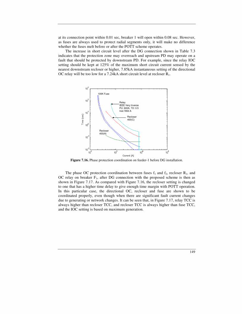
149
at its connection point within 0.01 sec, breaker 1 will open within 0.08 sec. However, as fuses are always used to protect radial segments only, it will make no difference whether the fuses melt before or after the POTT scheme operates. The increase in short circuit level after the DG connection shown in Table 7.3 indicates that the protection zone may overreach and upstream PD may operate on a fault that should be protected by downstream PD. For example, since the relay IOC setting should be kept at 125% of the maximum short circuit current sensed by the nearest downstream recloser or higher, 7.85kA instantaneous setting of the directional OC relay will be too low for a 7.24kA short circuit level at recloser R1.
RelayIEEE Very InversePU: 600A, TD: 0.5Inst:7850 A
100K Fuse
Recloser400(A)
Recloser400(C)
RelayIEEE Very InversePU: 600A, TD: 0.5Inst:7850 A
100K Fuse
Recloser400(A)
Recloser400(C)
Figure 7.16. Phase protection coordination on feeder-1 before DG installation.
The phase OC protection coordination between fuses f1 and f2, recloser R1, and OC relay on breaker F1, after DG connection with the proposed scheme is then as shown in Figure 7.17. As compared with Figure 7.16, the recloser setting is changed to one that has a higher time delay to give enough time margin with POTT operation. In this particular case, the directional OC, recloser and fuse are shown to be coordinated properly, even though when there are significant fault current changes due to generating or network changes. It can be seen that, in Figure 7.17, relay TCC is always higher than recloser TCC, and recloser TCC is always higher than fuse TCC, and the IOC setting is based on maximum generation.
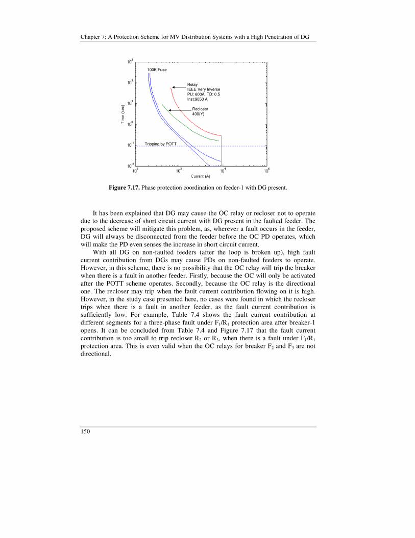
Chapter 7: A Protection Scheme for MV Distribution Systems with a High Penetration of DG
150
RelayIEEE Very InversePU: 600A, TD: 0.5Inst:9050 A
100K Fuse
Recloser400(Y)
Tripping by POTT
Figure 7.17. Phase protection coordination on feeder-1 with DG present.
It has been explained that DG may cause the OC relay or recloser not to operate due to the decrease of short circuit current with DG present in the faulted feeder. The proposed scheme will mitigate this problem, as, wherever a fault occurs in the feeder, DG will always be disconnected from the feeder before the OC PD operates, which will make the PD even senses the increase in short circuit current. With all DG on non-faulted feeders (after the loop is broken up), high fault current contribution from DGs may cause PDs on non-faulted feeders to operate. However, in this scheme, there is no possibility that the OC relay will trip the breaker when there is a fault in another feeder. Firstly, because the OC will only be activated after the POTT scheme operates. Secondly, because the OC relay is the directional one. The recloser may trip when the fault current contribution flowing on it is high. However, in the study case presented here, no cases were found in which the recloser trips when there is a fault in another feeder, as the fault current contribution is sufficiently low. For example, Table 7.4 shows the fault current contribution at different segments for a three-phase fault under F1/R1 protection area after breaker-1 opens. It can be concluded from Table 7.4 and Figure 7.17 that the fault current contribution is too small to trip recloser R2 or R3, when there is a fault under F1/R1
protection area. This is even valid when the OC relays for breaker F2 and F3 are not directional.
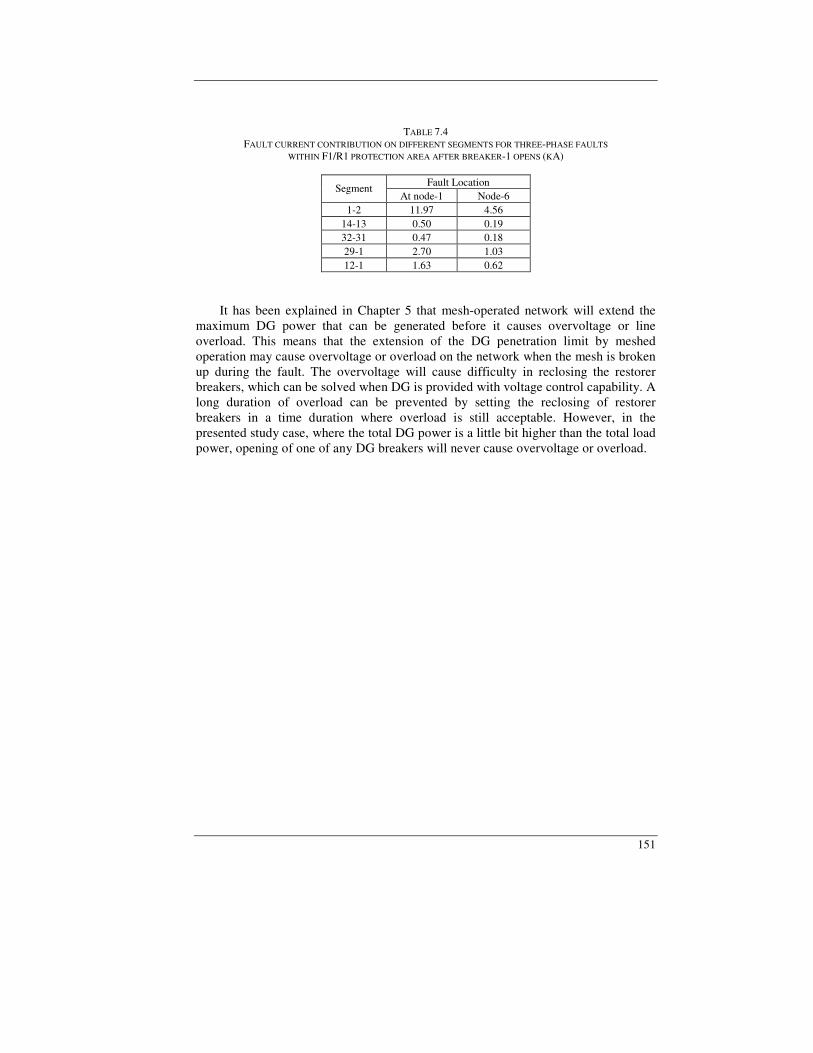
151
TABLE 7.4 FAULT CURRENT CONTRIBUTION ON DIFFERENT SEGMENTS FOR THREE-PHASE FAULTS
WITHIN F1/R1 PROTECTION AREA AFTER BREAKER-1 OPENS (KA) Fault Location Segment
At node-1 Node-6 1-2 11.97 4.56
14-13 0.50 0.19 32-31 0.47 0.18 29-1 2.70 1.03 12-1 1.63 0.62
It has been explained in Chapter 5 that mesh-operated network will extend the maximum DG power that can be generated before it causes overvoltage or line overload. This means that the extension of the DG penetration limit by meshed operation may cause overvoltage or overload on the network when the mesh is broken up during the fault. The overvoltage will cause difficulty in reclosing the restorer breakers, which can be solved when DG is provided with voltage control capability. A long duration of overload can be prevented by setting the reclosing of restorer breakers in a time duration where overload is still acceptable. However, in the presented study case, where the total DG power is a little bit higher than the total load power, opening of one of any DG breakers will never cause overvoltage or overload.

Chapter 7: A Protection Scheme for MV Distribution Systems with a High Penetration of DG
152
7.6 Conclusions A protection scheme to mitigate protection problems due to a high penetration of DG in distribution networks and keeping DG on line to supply loads during the fault has been proposed. It has been shown that, with the proposed scheme, it is possible to avoid unnecessary disconnection of DG. Moreover, no parts of the network are subjected to islanded operation and the conventional OC protective devices do not loose their functions and their proper coordination. The proposed protection scheme may lengthen the duration of fault, which will affect the dynamic performance of the system. The dynamic performance of the system has not been investigated in this thesis. All protection settings of the proposed scheme are based on off-line simulations and worst case conditions. The breakers that will be tripped in the first task, and which breaker will be the restorer breaker, are decided in advance. The performance of the proposed scheme can be improved with adaptive settings and decisions, such as:
• The settings are adjusted adaptively according to generation and network configuration changes;
• The breaker that will be tripped in the first task of the scheme is adaptively decided based on the location of the fault;
• When a fault occurs at a certain location that may lead to instability for a longer fault clearing, all breakers in the fault area can be tripped in the first task of the scheme.
Chapter 8
Conclusions and Future Work
8.1 Conclusions
In this thesis, the impact of distributed generation (DG) on steady state operation and control of power distribution systems have been investigated. Various factors that have led to an increased interest in DG schemes, and how DG is gaining more and more attention worldwide as an alternative to large-scale central generating stations, have been presented in Chapter 1.
Different DG technologies have been treated briefly in Chapter 2. Generator technologies, potentials and challenges, typical sizes, and power output controllability of each DG technology have been discussed. It has been shown that a number of DG technologies are in a position to compete with central generating stations. There are also likely opportunities for renewable energy technologies in DG, though some renewable energy based DG technologies are not yet generally cost-competitive nowadays.
The DG impact on voltage profiles and losses in low voltage (LV) feeders has been investigated in Chapter 3. Main conclusions of this chapter are: DG will increase the voltage profile along the feeder, which may lead to an overvoltage when the DG power is high; the overvoltage can be mitigated by allowing DG to absorb reactive power from the grid (reactive power absorption); controlled reactive power absorption by the DG can significantly increase maximum DG power that can be injected to the feeder (DG integration limit), with the disadvantage that it will increase feeder losses. Based on those conclusions, a DG operation mode has then been proposed. Further, two methods to calculate the voltage profile along LV feeders, i.e. the approximate method (AM) and loss summation method (LSM) have also been presented. It is shown that the voltage profile along LV feeders, for any possible feeder configuration, can be calculated accurately with LSM. On the other hand, the well-known linear approximation for voltage calculation may lead to gross underestimation of the maximum voltage variation along the feeder. The calculation has been extended to the derivation of simplified expressions to obtain DG size that causes the losses on a feeder, with certain configurations, to be a minimum or to be unchanged.
Chapter 8: Conclusions and Future Work
154
Voltage profile and losses in a LV feeder when both the DG source and load power stochastically vary have been analyzed in Chapter 4. It is shown that when DG and load power fluctuate throughout the day, a DG integration limit based on maximum DG and minimum load scenario will lead to unnecessary restrictions of the DG integration. Stochastic assessment using Monte Carlo simulations is shown to be a more reliable method. Further, when the DG is intended to deliver as much power as possible, this approach makes it possible to define an acceptable risk of overload that the DG owner may accept in order to install DG of higher rating.
Analysis of voltage control on MV networks in the presence of DG has been carried out in Chapter 5. The principle operation of on-load tap changer (LTC) and line drop compensation (LDC) has been reviewed. The result indicated that voltage control with LTC is reliable against DG, but DG may affect the effectiveness of the voltage control performed by LDC. Different voltage regulation methods (LTC with reduced setting, LTC with LDC, DG with reactive power control capability, VR installation and feeder operation in loop) have been investigated. The results show that the DG integration limit obtained by decreasing the LTC setting is very marginal. The activation of the LDC feature, which is present in most LTCs but often not used, can significantly increase the DG integration limit without disrupting voltage regulation on all load conditions, as long as a proper commissioning and a set of off-line simulations are conducted. The DG integration limit can also be extended by: operating DG at leading power factor, which implies additional reactive power flowing from the substation to the DG; VR installation, which means additional investment cost; or operating the feeders in closed-loops.
The impact of DG on short circuit, voltage dip, and overcurrent (OC) protection has been presented in Chapter 6. It has been shown that short circuit currents will increase with the presence of DG, but the short circuit currents sensed by protective devices (PDs) can either increase or decrease with the presence of DG. The increase or decrease of short circuit currents sensed by PDs may lead to protection problems, such as: mal-coordination between instantaneous overcurrent (IOC) relay and downstream recloser/fuse, time overcurrent (TOC) relay does not sense high impedance faults, mal-coordination between recloser and fuse and IOC relay operates due to faults on adjacent feeders; which needs appropriate corrective actions. It has been shown that DG always increases voltage the residual voltage during the dip. However, though DG can increase the residual voltage significantly, sometimes the increase is not enough to mitigate the voltage dip problem, i.e. preventing sensitive equipment (SE) from tripping.
Finally, a protection scheme to mitigate protection problems due to a high penetration of DG in distribution networks, whilst keeping DG on line to supply loads during the fault has been proposed in Chapter 7. It has been shown that, with the proposed scheme, it is possible to avoid unnecessary disconnection of DG. Moreover, no part of the network is subjected to islanded operation and the conventional OC protective devices do not loose their functions and their proper coordination.

155
8.2 Future Work
The impact of DG on steady state operation and control of power distribution systems has been investigated in this thesis. Slightly different topics have been addressed. There are two possible approaches for the continuation of the work. The first approach is moving from steady state to dynamics and islanding operation of power distribution systems. The second approach is going deeper into the topics that have been studied in this thesis. When the first approach is preferred, some research directions can be: Dynamics and stability of power systems with a high penetration of distributed generation
The presence of power electronic interfaces in fuel cells, photovoltaic panels, microturbines; or the presence of induction generators in wind power and small hydropower characterizes a new type of power system when compared with conventional systems using synchronous generators. The dynamic behavior of a system with low inertia, comprising some small sources with slow responses to control systems, is also quite different from traditional power systems [98]. Analytical tools for studying the dynamic properties of a power system with non synchronous generators and small sources are deemed necessary. Islanding operation
Unintentional islanding may cause a safety hazard to the utility personnel and the public, may increase quality problems of electric service to the utility customers, and causes serious damages to the DG if utility power is wrongly restored [99]-[100]. A study on islanding detection methods to detect the loss of utility supply in order to be able to promptly disconnect the DG from power grid as soon as possible is needed.
(Intentional) islanding operation demands additional technical requirements such as a large increase in protection complexity and specific frequency and voltage regulation capabilities from DG units. While voltage regulation capability is somewhat more frequent in DG units, frequency regulation is not that usual [101]. The islanding operation needs either the reduction of DG power or loads in order to reach balance load and generation in the system. Thus, besides the assessment of dynamical performance of DG units, assessments on protection system, frequency regulation with DG units and its coordination with under frequency load shedding are required in order to be able to put the system in islanding smoothly.

Chapter 8: Conclusions and Future Work
156
On the other hand, when the second approach is preferred, some research directions can be: Optimal voltage control coordination between LTCs, fixed and controllable shunt capacitors, and distributed generation
Voltage control in a MV feeder presented in Chapter 5 has not taken into account the sequence of the voltage regulation performed by different voltage control equipment. Further study that brings the results closer to the actual operation condition can be performed by considering the sequence of the events. For example, coordination between LTC, controllable shunt capacitors and DG (with voltage control capability) can be performed by using a three-step control method with each step acts at a different time constant: • Primary voltage control is performed by automatic voltage regulator (AVR). • The secondary voltage control is performed by LTC. • The tertiary voltage control is performed by controllable shunt capacitors. Further, optimal voltage control coordination can be achieved by setting different objective, such as losses minimization, reactive power transfer minimization, DG power output maximization, economic dispatch, etc. Implementation of the optimal voltage control coordination in an actual system
One important factor for the implementation of the proposed optimal voltage control coordination in an actual system is the accuracy of the system parameters, such as resistance and reactance of the line, DGs and loads. Further, the future system, in addition to the present condition, should also be captured. An effective way to obtain system parameters using available tools and to predict future conditions needs to be developed. Further work on protection systems
Mitigating the DG impact on overcurrent (OC) protection coordination by manual readjustment of OC relay settings will not be effective when the change of maximum and minimum DG in the system occurs quite often. One possible solution is to develop adaptive OC protection, when the feeder is kept operating in a radial system.
It has been mentioned in Chapter 7 that the dynamic performance of the system has not been taken into account in the study. Meanwhile, the proposed protection scheme may lengthen the duration of the fault, which will affect the dynamic performance of the system. Thus, the dynamic performance of the system with the proposed protection scheme needs studying. Further, the proposed protection scheme in Chapter 7 is based on off-line simulation. Further work can be carried out to improve the performance of the proposed scheme by using adaptive settings and decisions, based on actual operation and fault conditions.

References [1] A.R. Bergen and V. Vittal, Power System Analysis, Prentice Hall, 2000.
[2] T.A. Short, Electric Power Distribution Handbook, CRC Press LLC, 2004.
[3] Math Bollen, Voltage Control and Short Circuits in Power Systems, Teaching Compendium, Chalmers University of Technology, Gothenburg, Sweden, 2002.
[4] N. Jenkins, R. Allan, P. Crossley, D. Kirschen, G. Strbac, Embedded Generation, The Institution of Electrical Engineers, London, 2000.
[5] “Kyoto Protocol to the United Nations Framework Convention on Climate Change”. Available at http://unfccc.int/resource/docs/convkp/kpeng.html, last accessed 13 July 2005.
[6] CIRED preliminary report of CIRED Working Group 04, “Dispersed Generation”. Issued at the CIRED Conference in Nice, June 1999.
[7] A. Schweer, “Special Report Session 3”, in Proc. of CIGRE Symposium on Impact of demand side management, integrated resource planning and distributed generation, Neptun, Romania, 1997.
[8] A.J. Petrella, “Issues, impacts and strategies for distributed generation challenged power systems”, in Proc. of CIGRE Symposium on Impact of demand side management, integrated resource planning and distributed generation, Neptun, Romania, 1997.
[9] T. Ackermann, G. Andersson and L. Söder, “Distributed Generation: a definition”, Electric Power Systems Research, vol.57, 2001, pp. 195-204.
[10] A. Borbely and J.F. Kreider, Distributed Generation: A New Paradigm for the New Millenium”, CRC Press, 2001.
[11] IEA, Distributed Generation in Liberalised Electricity Markets, International Energy Agency, France. 2002.
[12] The European Wind Energy Association, press release on January 28, 2005, “Wind power continues to grow in 2004 in the EU, but faces constraints of grid and administrative barriers”. Available [online] at http://www.ewea.org/, last accessed 8 September 2005.
[13] The UK White Paper, February 2003. Available [online] at http://www.dti.gov.uk/energy/ whitepaper/ourenergyfuture.pdf, last accessed 13 July 2005.
[14] IEA, Renewable Energy, Market and Policy Trends in IEA Countries, International Energy Agency, France. 2004.
References
158
[15] P.M. Anderson, Power System Protection, IEEE Press, 1999.
[16] J.L. Blackburn, Protective Relaying Principles and Applications, Marcel Dekker, 1988.
[17] P.B. Barker, R.W. de Mello, ”Determining the Impact of Distributed Generation on Power Systems: Part I - Radial Distribution Systems”, in Proc. of 2000 IEEE PES Summer Meeting, vol.3, pp. 1645 – 1656.
[18] T.H. Boutsika, S. Papathanassiou and N. Drossos,” Calculation of the Fault Level Contribution of Distributed Generation According to IEC Standard 60909”, in Proc. of 2005 CIGRE Symposium on Power Systems with Dispersed Generation.
[19] IEA, Electric Power Technology: Opportunities and Challenges of Competition, International Energy Agency, France. 1999.
[20] T. Bray, “Distributed Gas Turbines.” Independent Energy, January/February 1999, pp. 44-46.
[21] J. Makansi, “Venerable engine/generator repositioned for on-site distributed power.” Power, January/February 1999, pp. 20-28.
[22] J.A. Oliver, “Generation Characteristics Task Force, CIGRE, Study Committees 11, 37, 38 and 39”, Electra, August 1999, No. 185, pp. 15 – 33.
[23] N. Jenkins, “Embedded Generation Tutorial”, Power Engineering Journal, June 1995, pp. 145 – 150.
[24] D.S. Henderson,” Synchronous or Induction Generators ? – The Choice for Small Scale Generation”, in Proc. of Opportunities and Advances in International Power Generation, 1996.
[25] IEA, Renewables for Power Generation: Status and Prospects, International Energy Agency, France. 2003.
[26] Y. Goswami, F. Kreith, and J Kreider, Principles of Solar Engineering, Taylor and Francis, New York, 2000.
[27] M.R. Patel, Wind and Solar Power Systems, CRC Press, 1999.
[28] D. A. Spera, “Wind Turbine Technology,” American Society of Mechanical Engineers, New York, 1994.
[29] IEEE Std. 1159-1995, IEEE Recommended Practice for onitoring Electric Power Quality.
[30] European Standard EN-50160, Voltage Characteristics of Electricity Supplied by Public Distribution Systems, CENELEC, Brussels, 1994.
[31] C.L. Masters, “Voltage rise the big issue when connecting embedded generation to long 11 kV overhead lines”, Power Engineering Journal, vol.16, Feb. 2002, pp. 5-12.
159
[32] S. Conti, S. Raiti, G. Tina, U. Vagliasindi, “Study of the impact of PV generation on voltage profile in LV distribution networks”, in Proc. of 2001 IEEE Porto Power Tech Conf., vol.4, pp.6.
[33] S. Conti, S. Raiti, G. Tina, U. Vagliasindi,” Distributed Generation in LV Distribution Networks: Voltage and Thermal Constraints”, in Proc. of 2003 IEEE Bologna Power Tech Conf., vol. 2.
[34] S. Persaud, B. Fox, and D. Flynn, ”Impact of remotely connected wind turbines on steady state operation of radial distribution networks”, IEE Proceedings – Generation, Transmission and Distribution, vol.147, no.3, May 2000.
[35] N.C. Scott, D.J. Atkinson, and J.E. Morrell, “Use of Load Control to Regulate Voltage on Distribution Networks with Embedded Generation”, IEEE Transactions on Power Systems, vol.17, no.2, May 2002, pp.510 – 515.
[36] B. Lindgren, Power-generation, Power-electronics and Power-systems issues of Power Converters for Photovoltaic Applications, PhD Thesis, Chalmers University of Technology, Sweden, 2002.
[37] P.A. Daly, J. Morrison, “Understanding the potential benefits of distributed generation on power delivery systems”, in Proc. of 2001 Rural Electric Power Conference, 29 April-1 May 2001, pp.A2-1-A2-13.
[38] Simpow®: Software for simulation of power systems. Available at: http://www.stri.se/metadot/index.pl?id=2221&isa=Category&op=show, last accessed September 2005.
[39] Central Station Engineers of the Westinghouse Electric Corporation. Electrical Transmission and Distribution Reference Book, Westinghouse Electric Corporation, Pennsylvania. 1964.
[40] E.B. Kurtz, T.M. Shoemaker, J.E. Mack, The lineman's and cableman's handbook, McGraw-Hill, New York, 1997.
[41] V. Cataliotti, Impianti Elettrici, S.F. Flaccovio, Palermo, 1984. (in Italian)
[42] T. Ackerman, V. Knyazkin, “Interaction between Distributed Generation and the Distribution Network: Operation Aspects”, in Proc. of 2002 IEEE/PES Asia Pacific Transmission and Distribution Conference and Exhibition, vol.2, pp.1357 – 1362.
[43] J. Mutale, G. Strbac, N. Jenkins, ”Allocation of losses in distribution systems with embedded generation”, IEE Proc.-Gener. Transm. Distrib., vol.147, no.1, January 2000, pp.7-14.
[44] V.H. Mendez, et.all, ”A Monte Carlo Approach for Assessment of Investments Deferral in Radial Distribution Networks with Distributed Generation”, in Proc. of 2003 IEEE PowerTech Conference, Bologna.
References
160
[45] G.B. Shrestha and L. Goel, ”A Study on Optimal Sizing of Stand-Alone Photovoltaic Stations”, IEEE Transactions on Energy Conversion, Vol. 13, No. 4, December 1998.
[46] S. Conti, T. Crimi, S. Raiti, G. Tina and U. Vagliasindi,” Probabilistic Approach to Assess the Performance of Grid-Connected PV Systems”, in Proc of 2002 International Conference on Probabilistic Methods Applied to Power Systems, Naples.
[47] H.A.M. Maghraby, M.H. Shwehdi and G.K. Al-Bassam, ”Probabilistic Assessment of Photovoltaic (PV) Generation Systems”, IEEE Transaction on Power Systems, vol. 17, no. 1, February 2002.
[48] R. Willington and W.Li, Reliability Assessment of Electric Power Systems Using Monte Carlo Methods, Plenum Press, 1994.
[49] G. Fishman, Monte Carlo: Concepts, Algorithms and Applications, Spinger, 1996.
[50] “Weather and Air Quality in Göteborg”. Available [online] at http://www.miljo.goteborg.se/luftnet/index-eng.htm, last accessed September 2nd, 2005.
[51] Sveriges Energiförsörjning, Elkraft Handboken: Elkraftsystem 1, Liber AB, Stockholm (in Swedish).
[52] R. Thomas, M. Fordham and Partners, Photovoltaics and Architecture, Spon Press, 2003.
[53] T. Gönen, Electric Power Distribution System, McGraw-Hill Book Company, 1986.
[54] J.H. Harlow, Electric Power Transformer Engineering, CRC Press, 2004.
[55] M. Thomson,” Automatic voltage control relays and embedded generation, part I”, Power Engineering Journal, vol. 14, pp. 71 – 76, April 2000.
[56] P. Brady, C. Dai and Y. Baghzouz, “Need to revise switched capacitor controls on feeders with distributed generation”, in Proc. of 2003 IEEE PES Transmission and Distribution Conference and Exposition, vol. 2, pp. 590 - 594.
[57] S. Repo, H. Laaksonen, et. al., ”A case study of voltage rise problem due to a large amount of distributed generation on a weak distribution network”, in Proc. of. 2003 IEEE Bologna PowerTech Conference, vol.4.
[58] T.E. Kim and J.E Kim, “A method for determining the introduction limit of distributed generation system in distribution system”, in Proc. of 2001 IEEE Power Engineering Society Summer Meeting, vol.1, pp. 456 – 461.
[59] L.A. Kojovic, “The impact of dispersed generation and voltage regulator operations on power quality”, in Proc. of CIGRE 2005 Athens Symposium.
161
[60] J.H. Choi and J.C. Kim, “Advanced voltage regulation method of power distribution systems interconnected with dispersed storage and generation systems”, IEEE Transactions on Power Delivery, vol.16, no.2, April 2001, pp.329-334.
[61] G. Celli, F. Pilo and G. Pisano, “Meshed Distribution Networks to Increase the Maximum Allowable Distributed Generation Capacity”, in Proc. of 2005 CIGRE Symposium.
[62] G. Celli, F. Pilo and G. Pisano, V. Allegranza, R. Cicoria and A. Iaria, “ Meshed vs. Radial MV Distribution Network in Presence of Large Amount of DG”, in Proc. of 2004 Power Systems Conference and Exposition, vol. 2, pp. 709 – 714.
[63] DIgSILENT PowerFactory, available at http://www.digsilent.de/
[64] Distribution System Analysis Subcommittee Report, “Radial distribution test feeders”, 2001 IEEE Power Engineering Society Winter Meeting, vol.2, pp. 908-912.
[65] IEC 61000-2-1:1990, “Electromagnetic Compatibility. Part 2: Environment. Section 1: Description of the environment – Electromagnetic environment for low frequency conducted disturbances and signaling in public power supply system”.
[66] IEEE Std 1346-1998, “IEEE recommended practice for evaluating electric power system compatibility with electronic process equipment”.
[67] S.M. Brahma and A.A. Girgis, “Development of Adaptive Protection Scheme for Distribution Systems with High Penetration of Distributed Generation”, IEEE Transactions on Power Delivery, vol. 19, no.1, January 2004.
[68] A.A. Girgis and S.M. Brahma, “Effect of Distributed Generation on Protective Device Coordination in Distribution System”, in Proc. of 2001 Large Engineering Systems Conference on Power Engineering, LESCOPE '01, pp.115-119.
[69] M.T. Doyle, “Reviewing the Impacts of Distributed Generation on Distribution System Protection”, in Proc. of 2002 Power Engineering Society Summer Meeting, vol.1, pp. 103-105.
[70] M. Baran and I. El-Markabi, “Adaptive Over Current Protection for Distribution Feeders with Distributed Generators”, in Proc. of 2004 Power Systems Conference and Exposition, vol. 2, pp. 715 – 719.
[71] K. Maki, P. Jarventausa and S. Rapo, “Protection Issues in Planning of Distribution Network Including Distributed Generation”, in Proc. of 2005 CIGRE Symposium.
[72] M.H.J. Bollen, Understanding Power Quality Problems, IEEE Press, 2000, pp. 139-324.
References
162
[73] E.R. Collins, Jr. and J. Jiang, ”The Role of a Synchronous Distributed Generator on Voltage Sags”, In Proc. Of 2004 International Conference on Harmonics and Power Quality.
[74] J.C. Gomez and M.M. Morcos, “Coordination of Voltage Sag and Overcurrent Protection in DG Systems”, IEEE Transaction on Power Delivery, vol. 20, no.1, January 2005, pp. 214-218.
[75] T. Gönen, Modern Power System Analysis, John Willey and Sons, 1987, pp. 218 – 225, 265 – 293.
[76] A.R. Bergen and V. Vittal, Power System Analysis, Prentice Hall, 2000.
[77] J. Daalder, Power System Analysis, Teaching Compendium, Chalmers University of Technology, Gothenburg, Sweden, 2004.
[78] M.H.J. Bollen and L.D. Zhang, “Different methods for classification of three-phase unbalanced voltage dips due to faults”, Electric Power Systems Research, vol. 66, 2003, pp. 59-69.
[79] CYMTCC, Protective Device Coordination. Available [online] at: http://www.cyme.com/software/cymtcc/
[80] IEEE Std C37.112-1996, “IEEE Standard Inverse-Time Characteristic Equations for Overcurrent Relays”.
[81] S.M. Brahma and A.A. Girgis, “Microprocessor-Based Reclosing to Coordinate Fuse and Recloser in a System with High Penetration of Distributed Generation”, in Proc. of 2002 Power Engineering Society Winter Meeting, vol.1, pp.453-458.
[82] ABB, Type R Outdoor Circuit Breakers Descriptive Bulletin, available at http://library.abb.com/GLOBAL/SCOT/scot235.nsf/VerityDisplay/C86D74F8BADF3C0785256B4100759DA7/$File/Type%20R%20Descriptive%20Bulletin.pdf, last accessed 17 January 2006.
[83] Square D, Powersub™ Medium Voltage Substation Circuit Breakers, Type FVR Brochures, available [online] at http://ecatalog.squared.com/pubs/Circuit%20Protection/Medium%20Voltage%20Circuit%20Breakers/Substation%20Circuit%20Breakers/6065/6065HO9601.pdf, last accessed 17 January 2006.
[84] J.C. Gomez and M.M. Morcos, “Voltage Sag and Recovery Time in Repetitive Events”, IEEE Transaction on Power Delivery, vol. 17, no.4, October 2002, pp. 1037-1043.
[85] R.S. Thallam and G.T. Heydt, “Power Acceptability and Voltage Sag Indices in the Three Phase Sense”, available [online] at http://grouper.ieee.org/groups/sag/IEEEP1564_00_10.ppt, last accessed 23 January 2006.
163
[86] “Technical Requirements for the Interconnection of Generation Resources”, Boneville Power Administration document. Available [online] at http://grouper.ieee.org/groups/spd/spdc_refernce_desk.htm. Last accessed 8 September 2005.
[87] “Invertie Protection of Customer Owned Resources of Generation 3 MVA or Less”, IEEE publication no. 88TH0224-6-PWR.
[88] M.H.J. Bollen and M. Häger,” Impact of Increasing Penetration of Distributed Generation on the Number of Voltage Dips Experienced by End-customers”, in Proc. of 2005 CIRED International Conference on Electricity Distribution.
[89] F.A. Magueed, On Power Electronics Interface for Distributed Generation Applications and its Impact on System Reliability to Customers, Licentiate Thesis, Chalmers University of Technology, Gothenburg, Sweden, 2005.
[90] I.M. Chilvers, N. Jenkins and P. Crossley, “The use of 11 kV Distance Protection to Increase Generation Connected to the Distribution Network”, in Proc. of. 2004 IEE International Conference on Developments in Power System Protection.
[91] L.K. Kumpulainen and K.T. Kauhaniemi, “Analysis of the impact of distributed generation on automatic reclosing”, in Proc. of. 2004 Power Systems Conference and Exposition, vol.1, pp. 603 – 608.
[92] A. Nikander, S. Repo and P. Järventausta, “Utilizing the Ring Operation Mode of Medium Voltage Distribution Feeders”, in Proc. of 2003 International Conference on Electricity Distribution CIRED.
[93] M. Jonsson, Line Protection and Power System Collapse, Licentiate Thesis, Chalmers University of Technology, Gothenburg, Sweden, 2001.
[94] W.A. Elmore, et.all., Protective Relaying Theory and Application, Marcel Dekker, Inc. 2004.
[95] W.A. Elmore, et.all., Pilot Protective Relaying, Marcel Dekker, Inc. 2000.
[96] GE Multilin, D60 Line Distance Relay, available [online] at http://www.geindustrial.com/cwc/products?pnlid=6&id=d60, last accessed 9 February 2006.
[97] ABB, REL 512 Numerical Transmission Line Protection System, available at http://library.abb.com/GLOBAL/SCOT/scot229.NSF/VerityDisplay/879DBAC43873291C85256F330062ED87/$File/DB41-440m%20%20%20%20REL512.pdf, last accessed 9 February 2006.
[98] J. A. Pecas Lopes, et. al., “Control Strategies for MicroGrids Emergency Operation, in Proc. of 2005 International Conference on Future Power Systems.
References
164
[99] T. Ackermann, G. Andersson, and L. Soder, “Electricity Market Regulations and their Impact on Distributed Generatiron,” in Proc. of 2000 International Conference on Electric Utility Deregulation and Restructuring and Power Technologies.
[100] O. Usta and M. A. Refern, “Protection of Dispersed Storage and Generation Units Against Islanding,” in Proc. of 1994 Mediterranean Electrotechnical Conference.
[101] L. Seca, and J. A. Pecas Lopes, “Intentional islanding for reliability improvement in distribution networks with high DG penetration”, in Proc. of 2005 International Conference on Future Power Systems.