Statistics for high-dimensional data:Introduction, and the Lasso for linear models

Peter Buhlmann and Sara van de Geer

Seminar fur Statistik, ETH Zurich

May 2012

High-dimensional dataRiboflavin production with Bacillus Subtilis

(in collaboration with DSM (Switzerland))goal: improve riboflavin production rate of Bacillus Subtilis

using clever genetic engineering

response variables Y ∈ R: riboflavin (log-) production ratecovariates X ∈ Rp: expressions from p = 4088 genessample size n = 115, p � n

gene expression data

Y versus 9 “reasonable” genes

7.6 8.0 8.4 8.8

−10

−9

−8

−7

−6

xsel

y

7 8 9 10 11 12

−10

−9

−8

−7

−6

xsel

y

6 7 8 9 10

−10

−9

−8

−7

−6

xsel

y

7.5 8.0 8.5 9.0

−10

−9

−8

−7

−6

xsel

y

7.0 7.5 8.0 8.5 9.0

−10

−9

−8

−7

−6

xsel

y

8 9 10 11

−10

−9

−8

−7

−6

xsel

y

8 9 10 11 12

−10

−9

−8

−7

−6

xsel

y

7.5 8.0 8.5 9.0

−10

−9

−8

−7

−6

xsel

y

8.5 9.0 9.5 10.0 11.0

−10

−9

−8

−7

−6

xsel

y

general framework:

Z1, . . . ,Zn (with some ”i.i.d. components”)dim(Zi)� n

for example:Zi = (Xi ,Yi), Xi ∈ X ⊆ Rp,Yi ∈ Y ⊆∈ R: regression with p � nZi = (Xi ,Yi), Xi ∈ X ⊆∈ Rp,Yi ∈ {0,1}: classification for p � n

numerous applications:biology, imaging, economy, environmental sciences, ...

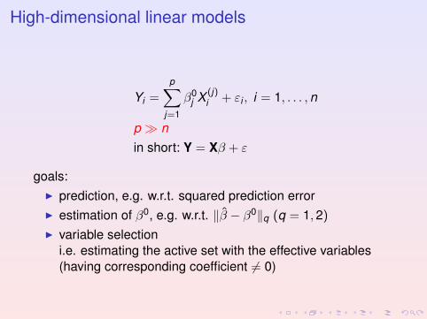
High-dimensional linear models

Yi =

p∑j=1

β0j X (j)

i + εi , i = 1, . . . ,n

p � nin short: Y = Xβ + ε

goals:I prediction, e.g. w.r.t. squared prediction errorI estimation of β0, e.g. w.r.t. ‖β − β0‖q (q = 1,2)

I variable selectioni.e. estimating the active set with the effective variables(having corresponding coefficient 6= 0)

we need to regularize...and there are many proposals

I Bayesian methods for regularizationI greedy algorithms: aka forward selection or boostingI preliminary dimension reductionI ...

e.g. 3’190’000 entries on Google Scholar for“high dimensional linear model” ...

we need to regularize...and there are many proposals

I Bayesian methods for regularizationI greedy algorithms: aka forward selection or boostingI preliminary dimension reductionI ...

e.g. 3’190’000 entries on Google Scholar for“high dimensional linear model” ...

we need to regularize...and there are many proposals

I Bayesian methods for regularizationI greedy algorithms: aka forward selection or boostingI preliminary dimension reductionI ...

e.g. 3’190’000 entries on Google Scholar for“high dimensional linear model” ...

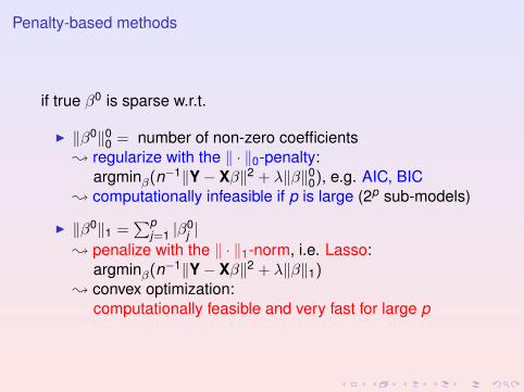
Penalty-based methods

if true β0 is sparse w.r.t.

I ‖β0‖00 = number of non-zero coefficients; regularize with the ‖ · ‖0-penalty:

argminβ(n−1‖Y− Xβ‖2 + λ‖β‖00), e.g. AIC, BIC; computationally infeasible if p is large (2p sub-models)

I ‖β0‖1 =∑p

j=1 |β0j |

; penalize with the ‖ · ‖1-norm, i.e. Lasso:argminβ(n−1‖Y− Xβ‖2 + λ‖β‖1)

; convex optimization:computationally feasible and very fast for large p

The Lasso (Tibshirani, 1996)

Lasso for linear models

β(λ) = argminβ(n−1‖Y− Xβ‖2 + λ︸︷︷︸≥0

‖β‖1︸ ︷︷ ︸Ppj=1 |βj |

)

; convex optimization problem

I Lasso does variable selectionsome of the βj(λ) = 0(because of “`1-geometry”)

I β(λ) is a shrunken LS-estimate

more about “`1-geometry”

equivalence to primal problem

βprimal(R) = argminβ;‖β‖1≤R‖Y− Xβ‖22/n,

with a correspondence between λ and R which depends on thedata (X1,Y1), . . . , (Xn,Yn)[such an equivalence holds since

I ‖Y− Xβ‖22/n is convex in βI convex constraint ‖β‖1 ≤ R

see e.g. Bertsekas (1995)]

p=2

left: `1-“world”residual sum of squares reaches a minimal value (for certainconstellations of the data) if its contour lines hit the `1-ball in itscorner; β1 = 0

`2-“world” is different

Ridge regression,

βRidge(λ) = argminβ

(‖Y− Xβ‖22/n + λ‖β‖22

),

equivalent primal equivalent solution

βRidge;primal(R) = argminβ;‖β‖2≤R‖Y− Xβ‖22/n,with a one-to-one correspondence between λ and R

A note on the Bayesian approach

model:

β1, . . . , βp i.i.d. ∼ p(β)dβ,given β : Y ∼ Nn(Xβ, σ2In) with density f (y|σ2, β)

posterior density:

p(β|Y, σ2) =f (Y|β, σ2)p(β)∫f (Y|β, σ2)p(β)dβ

∝ f (Y|β, σ2)p(β)

and hence for the MAP (Maximum A-Posteriori) estimator:

βMAP = argmaxβp(β|Y, σ2) = argminβ − log(

f (Y|β, σ2)p(β))

= argminβ

12σ2 ‖Y− Xβ‖22 −

p∑j=1

log(p(βj))

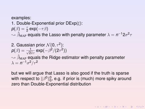
examples:1. Double-Exponential prior DExp(ξ):p(β) = τ

2 exp(−τβ)

; βMAP equals the Lasso with penalty parameter λ = n−12σ2τ

2. Gaussian prior N (0, τ2):p(β) = 1√

2πτexp(−β2/(2τ2))

; βMAP equals the Ridge estimator with penalty parameterλ = n−1σ2/τ2

but we will argue that Lasso is also good if the truth is sparsewith respect to ‖β0‖00, e.g. if prior is (much) more spiky aroundzero than Double-Exponential distribution

Orthonormal design

Y = Xβ + ε, n−1XT X = I

Lasso = soft-thresholding estimatorβj(λ) = sign(Zj)(|Zj | − λ/2)+, Zj︸︷︷︸

=OLS

= (n−1XT Y)j ,

βj(λ) = gsoft(Zj),

[this is Exercise 2.1]

−3 −2 −1 0 1 2 3

−3

−2

−1

01

23

threshold functions

z

Adaptive LassoHard−thresholdingSoft−thresholding

Prediction

goal: predict a new observation Ynewconsider expected (w.r.t. new data; and random X ) squarederror loss:

EXnew,Ynew [(Ynew − Xnewβ)2] = σ2 + EXnew [(Xnew(β0 − β))2]

= σ2 + (β − β0)T Σ︸︷︷︸Cov(X)

(β − β0)

; terminology “prediction error”:

for random design X: (β − β0)T Σ(β − β0) = EXnew [(Xnew(β − β0))2]

for fixed design X: (β − β0)T Σ(β − β0) = ‖X(β − β0)‖22/n

binary lymph node classification using gene expressions:a high noise problem

n = 49 samples, p = 7130 gene expressions

despite that it is classification: P[Y = 1|X = x ] = E[Y |X = x ]; p(x) via linear model; can then do classification

cross-validated misclassification error (2/3 training; 1/3 test)

Lasso L2Boosting FPLR Pelora 1-NN DLDA SVM

21.1% 17.7% 35.25% 27.8% 43.25% 36.12% 36.88%

with variable selection best 200 genes (Wilcoxon test)no additional variable selection

Lasso selected on CV-average 13.12 out of p = 7130 genes

from a practical perspective:if you trust in cross-validation: can validate how good we arei.e. prediction may be a black box, but we can evaluate it!

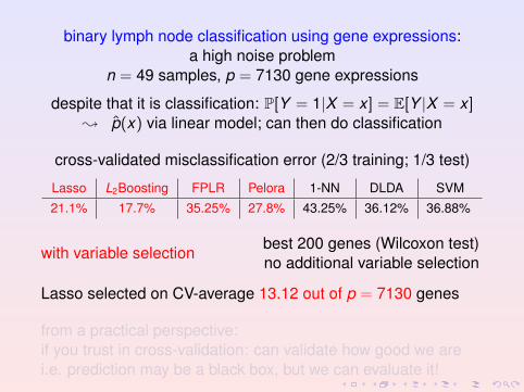
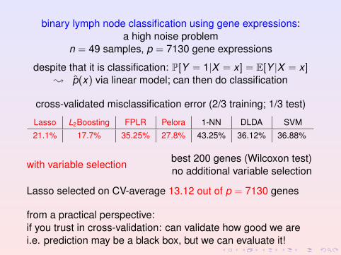
binary lymph node classification using gene expressions:a high noise problem

n = 49 samples, p = 7130 gene expressions

despite that it is classification: P[Y = 1|X = x ] = E[Y |X = x ]; p(x) via linear model; can then do classification

cross-validated misclassification error (2/3 training; 1/3 test)

Lasso L2Boosting FPLR Pelora 1-NN DLDA SVM

21.1% 17.7% 35.25% 27.8% 43.25% 36.12% 36.88%

with variable selection best 200 genes (Wilcoxon test)no additional variable selection

Lasso selected on CV-average 13.12 out of p = 7130 genes

from a practical perspective:if you trust in cross-validation: can validate how good we arei.e. prediction may be a black box, but we can evaluate it!

and in fact: we will hear thatI Lasso is consistent for prediction assuming “essentially

nothing”I Lasso is optimal for prediction assuming the “compatibility

condition” for X

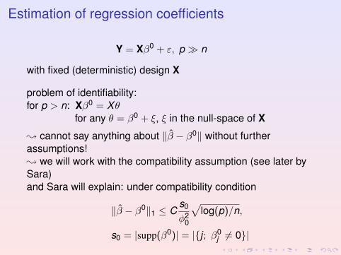
Estimation of regression coefficients

Y = Xβ0 + ε, p � n

with fixed (deterministic) design X

problem of identifiability:for p > n: Xβ0 = Xθ

for any θ = β0 + ξ, ξ in the null-space of X

; cannot say anything about ‖β − β0‖ without furtherassumptions!; we will work with the compatibility assumption (see later bySara)and Sara will explain: under compatibility condition

‖β − β0‖1 ≤ Cs0

φ20

√log(p)/n,

s0 = |supp(β0)| = |{j ; β0j 6= 0}|

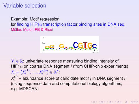
Variable selection

Example: Motif regressionfor finding HIF1α transcription factor binding sites in DNA seq.Muller, Meier, PB & Ricci

Yi ∈ R: univariate response measuring binding intensity ofHIF1α on coarse DNA segment i (from CHIP-chip experiments)Xi = (X (1)

i , . . . ,X (p)i ) ∈ Rp:

X (j)i = abundance score of candidate motif j in DNA segment i

(using sequence data and computational biology algorithms,e.g. MDSCAN)

question: relation between the binding intensity Y and theabundance of short candidate motifs?

; linear model is often reasonable“motif regression” (Conlon, X.S. Liu, Lieb & J.S. Liu, 2003)

Y = Xβ + ε, n = 287, p = 195

goal: variable selection; find the relevant motifs among the p = 195 candidates

Lasso for variable selection

S(λ) = {j ; βj(λ) 6= 0}for S0 = {j ;β0

j 6= 0}

no significance testing involvedit’s convex optimization only!

(and that can be a problem... see later)

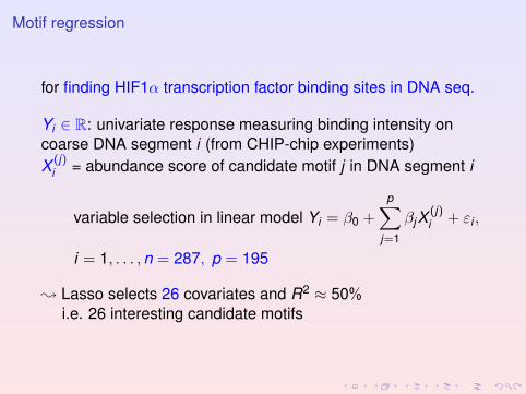
Motif regression

for finding HIF1α transcription factor binding sites in DNA seq.

Yi ∈ R: univariate response measuring binding intensity oncoarse DNA segment i (from CHIP-chip experiments)X (j)

i = abundance score of candidate motif j in DNA segment i

variable selection in linear model Yi = β0 +

p∑j=1

βjX(j)i + εi ,

i = 1, . . . ,n = 287, p = 195

; Lasso selects 26 covariates and R2 ≈ 50%i.e. 26 interesting candidate motifs

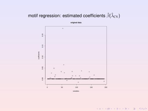
motif regression: estimated coefficients β(λCV)

0 50 100 150 200

0.00

0.05

0.10

0.15

0.20

original data

variables

coef

ficie

nts

“Theory” for variable selection with Lasso

for (fixed design) linear model Y = Xβ0 + ε withactive set S0 = {j ; β0

j 6= 0}two key assumptions

1. neighborhood stability condition for design X⇔ irrepresentable condition for design X

2. beta-min condition

minj∈S0|β0

j | ≥ C√

s0 log(p)/n, C suitably large

both conditions are sufficient and “essentially” necessary for

S(λ) = S0 with high probability, λ�√

log(p)/n︸ ︷︷ ︸larger than for pred.

already proved in Meinshausen & PB, 2004 (publ: 2006)and both assumptions are restrictive!

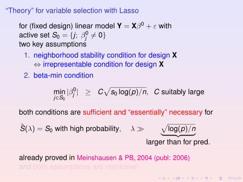
“Theory” for variable selection with Lasso

for (fixed design) linear model Y = Xβ0 + ε withactive set S0 = {j ; β0

j 6= 0}two key assumptions

1. neighborhood stability condition for design X⇔ irrepresentable condition for design X

2. beta-min condition

minj∈S0|β0

j | ≥ C√

s0 log(p)/n, C suitably large

both conditions are sufficient and “essentially” necessary for

S(λ) = S0 with high probability, λ�√

log(p)/n︸ ︷︷ ︸larger than for pred.

already proved in Meinshausen & PB, 2004 (publ: 2006)and both assumptions are restrictive!

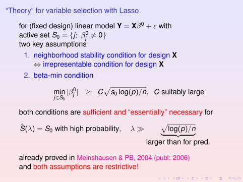
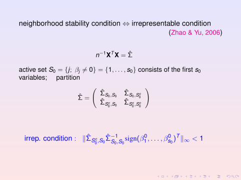
neighborhood stability condition⇔ irrepresentable condition(Zhao & Yu, 2006)

n−1XT X = Σ

active set S0 = {j ; βj 6= 0} = {1, . . . , s0} consists of the first s0variables; partition

Σ =

(ΣS0,S0 ΣS0,Sc

0

ΣSc0 ,S0 ΣSc

0 ,Sc0

)

irrep. condition : ‖ΣSc0 ,S0

Σ−1S0,S0

sign(β01 , . . . , β

0s0

)T‖∞ < 1

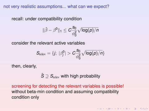
not very realistic assumptions... what can we expect?

recall: under compatibility condition

‖β − β0‖1 ≤ Cs0

φ20

√log(p)/n

consider the relevant active variables

Srelev = {j ; |β0j | > C

s0

φ20

√log(p)/n}

then, clearly,

S ⊇ Srelev with high probability

screening for detecting the relevant variables is possible!without beta-min condition and assuming compatibilitycondition only

in addition: assuming beta-min condition

minj∈S0|β0

j | > Cs0

φ20

√log(p)/n

S ⊇ S0 with high probability

screening for detecting the true variables

Tibshirani (1996):LASSO = Least Absolute Shrinkage and Selection Operator

new translation:LASSO = Least Absolute Shrinkage and Screening Operator

Practical perspective

choice of λ: λCV from cross-validationempirical and theoretical indications (Meinshausen & PB, 2006)that

S(λCV ) ⊇ S0 (or Srelev)

moreover

|S(λCV )| ≤ min(n,p)(= n if p � n)

; huge dimensionality reduction (in the original covariates)

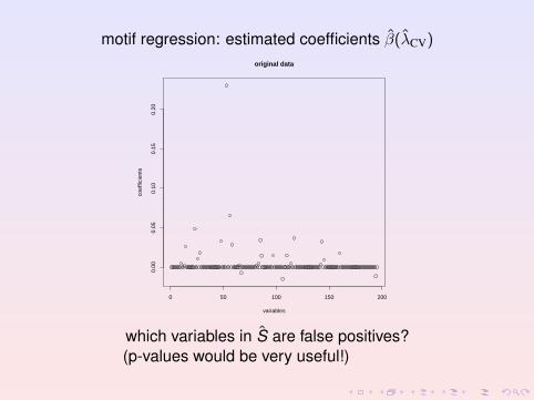
motif regression: estimated coefficients β(λCV)

0 50 100 150 200

0.00

0.05

0.10

0.15

0.20

original data

variables

coef

ficie

nts

which variables in S are false positives?(p-values would be very useful!)

recall:

S(λCV ) ⊇ S0 (or Srelev)

and we would then use a second-stage to reduce the numberof false positive selections

; re-estimation on much smaller model with variables from SI OLS on S with e.g. BIC variable selectionI thresholding coefficients and OLS re-estimationI adaptive Lasso (Zou, 2006)I ...

recall:

S(λCV ) ⊇ S0 (or Srelev)

and we would then use a second-stage to reduce the numberof false positive selections

; re-estimation on much smaller model with variables from SI OLS on S with e.g. BIC variable selectionI thresholding coefficients and OLS re-estimationI adaptive Lasso (Zou, 2006)I ...

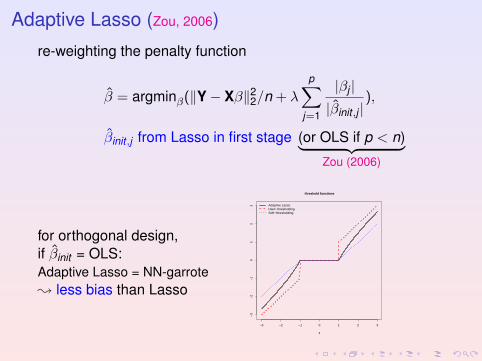
Adaptive Lasso (Zou, 2006)

re-weighting the penalty function

β = argminβ(‖Y− Xβ‖22/n + λ

p∑j=1

|βj ||βinit ,j |

),

βinit ,j from Lasso in first stage (or OLS if p < n)︸ ︷︷ ︸Zou (2006)

for orthogonal design,if βinit = OLS:Adaptive Lasso = NN-garrote; less bias than Lasso

−3 −2 −1 0 1 2 3

−3

−2

−1

01

23

threshold functions

z

Adaptive LassoHard−thresholdingSoft−thresholding

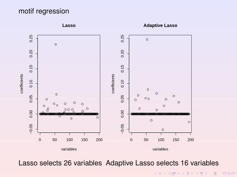
motif regression

0 50 100 150 200

−0.

050.

000.

050.

100.

150.

200.

25Lasso

variables

coef

ficie

nts

0 50 100 150 200

−0.

050.

000.

050.

100.

150.

200.

25

Adaptive Lasso

variables

coef

ficie

nts

Lasso selects 26 variables Adaptive Lasso selects 16 variables

KKT conditions and Computationcharacterization of solution(s) β as minimizer of the criterionfunction

Qλ(β) = ‖Y− Xβ‖22/n + λ‖β‖1

since Qλ(·) is a convex function:necessary and sufficient that subdifferential of ∂Qλ(β)/∂β at βcontains the zero element

Lemma 2.1 first part (in the book)denote by G(β) = −2XT (Y− Xβ)/n the gradient vector of‖Y− Xβ‖22/nThen: β is a solution if and only if

Gj(β) = −sign(βj)λ if βj 6= 0,

|Gj(β)| ≤ λ if βj = 0

Lemma 2.1 second part (in the book)If the solution of argminβQλ(β) is not unique (e.g. if p > n), andif Gj(β) < λ for some solution β, then βj = 0 for all (other)solutions β in argminβQλ(β).

The zeroes are “essentially” unique(“essentially” refers to the situation: βj = 0 and Gj(β) = λ)

Proof: Exercise (optional), or see in the book

Coordinate descent algorithm for computation

general idea is to compute a solution β(λgrid,k ) and use it as astarting value for the computation of β(λgrid,k−1︸ ︷︷ ︸

<λgrid,k

)

β(0) ∈ Rp an initial parameter vector. Set m = 0.

REPEAT:Increase m by one: m← m + 1.For j = 1, . . . ,p:

if |Gj(β(m−1)−j )| ≤ λ : set β(m)

j = 0,

otherwise: β(m)j = argminβj

Qλ(β(m−1)+j ),

β−j : parameter vector setting j th component to zeroβ

(m−1)+j : parameter vector which equals β(m−1) except for j th

component equalling βjUNTIL numerical convergence

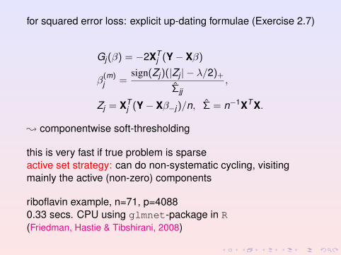
for squared error loss: explicit up-dating formulae (Exercise 2.7)

Gj(β) = −2XTj (Y− Xβ)

β(m)j =

sign(Zj)(|Zj | − λ/2)+

Σjj,

Zj = XTj (Y− Xβ−j)/n, Σ = n−1XT X.

; componentwise soft-thresholding

this is very fast if true problem is sparseactive set strategy: can do non-systematic cycling, visitingmainly the active (non-zero) components

riboflavin example, n=71, p=40880.33 secs. CPU using glmnet-package in R(Friedman, Hastie & Tibshirani, 2008)

coordinate descent algorithm converges to a stationary point(Paul Tseng ≈ 2000); convergence to a global optimum, due to convexity of theproblem

main assumption:

objective function = smooth function + penalty︸ ︷︷ ︸separable

here: “separable” means “additive”, i.e., pen(β) =∑p

j=1 pj(βj)

failure of coordinate descent algorithm:Fused Lasso

β = argminβ‖Y− Xβ‖22/n + λ

p∑j=2

|βj − βj−1|+ λ2‖β‖1

but∑p

j=2 |βj − βj−1| is non-separable

contour lines of penalties for p = 2|beta1 − beta2|

beta1

beta

2

0.5

0.5

1

1

1.5

1.5

2

2

2.5

2.5

3

3

3.5

3.5

−2 −1 0 1 2

−2

−1

01

2

|beta1| + |beta2|

beta1

beta

2 0.5

1

1.5

2

2.5

2.5

2.5

2.5

3

3

3

3

3.5

3.5

3.5

3.5

−2 −1 0 1 2

−2

−1

01

2