Embed Size (px)
Citation preview
The Florida State UniversityDigiNole Commons
Electronic Theses, Treatises and Dissertations The Graduate School
12-14-2007
Statistical Modeling of Small-Scale FadingChannelsMahinga Leandra HekenoFlorida State University
Follow this and additional works at: http://diginole.lib.fsu.edu/etd
This Thesis - Open Access is brought to you for free and open access by the The Graduate School at DigiNole Commons. It has been accepted forinclusion in Electronic Theses, Treatises and Dissertations by an authorized administrator of DigiNole Commons. For more information, please [email protected].
Recommended CitationHekeno, Mahinga Leandra, "Statistical Modeling of Small-Scale Fading Channels" (2007). Electronic Theses, Treatises and Dissertations.Paper 4134.
THE FLORIDA STATE UNIVERSITY
FAMU – FSU COLLEGE OF ENGINEERING
STATISTICAL MODELING OF SMALL-SCALE FADING CHANNELS
By
MAHINGA HEKENO
A Thesis submitted to the Department of Electrical Engineering
in partial fulfillment of the requirements for the degree of
Master of Science
Degree Awarded: Spring Semester, 2008
Copyright © 2007 Mahinga Hekeno
All Rights Reserved
ii
The members of the Committee approve the thesis of Mahinga Hekeno defended on
December 14th, 2007
________________________
Bing W. Kwan
Professor Directing Thesis
________________________
Ming Yu
Committee Member
________________________
Krishna Arora
Committee Member
Approved:
______________________________________
Victor DeBrunner, Chair, Department of Electrical and Computer Engineering
______________________________________
Ching-Jen Chen, Dean, FAMU-FSU College of Engineering
The Office of Graduate Studies has verified and approved the above named committee
members.

iii
In Memory of Jennifer Marealle-Hekeno
iv
ACKNOWLEDGMENTS
I would like to express my sincere gratitude to my supervisor Dr. Bing W. Kwan for his
valuable guidance and continuous support throughout my graduate program. His tireless
efforts and willingness to share his in-depth knowledge and experience provided me with
essential ingredients for my academic development. Furthermore, I would like to thank
my committee members, Dr. Krishna Arora and Dr. Ming Yu, for their willingness to be
part of the thesis committee and their generous advice and interest.
I would like to say a special thanks to Dr. Primus Mtenga for his financial support that
facilitated the completion of my graduate studies.
I would also like to thank the academic and administrative staff in the Department of
Electrical and Computer Engineering as well as my colleagues at the Information
Processing and Transmission Engineering laboratory (IPTEL); Hung Khong, Hai Hoang,
Ma Xiaoguang, Turgay Koklu, Khue Ngo and Robert Hunter.
Furthermore, I would like to thank all the friends I have met over my years at Florida
State University; especially, Donation Mkubulo, Wolta Shiyo, Dr. Victor Mchuruza,
Doreen Kobelo, Saidi Siuhi, Judith Lwitiko, Cathbert Akaro and Geophrey Mbatta. I
have learned a lot from each of you.
Finally, I would like to thank my family for believing in me.
v
TABLE OF CONTENTS
LIST OF TABLES............................................................................................................ vii
LIST OF FIGURES ......................................................................................................... viii
ABSTRACT...................................................................................................................... xii
1. INTRODUCTION ...................................................................................................... 1
1.1. Overview............................................................................................................. 1
1.2. Background......................................................................................................... 1
1.3. Scope of Work .................................................................................................... 2
1.3.1. The Communication System.......................................................................2
2. DETERMINATION OF THE PHYSICS-BASED CHANNEL MODEL................. 4
2.1. Multipath Channel Characterization................................................................... 4
2.2. Linear Time-Varying Channel............................................................................ 4
2.2.1. Doppler Shift............................................................................................... 5
2.2.2. Multipath Delay .......................................................................................... 6
2.2.3. The Field Strength Amplitude .................................................................... 6
2.3. Development of the Physics-based channel Model............................................ 9
2.4. The Simulation Model ...................................................................................... 12
2.4.1. Channel Space........................................................................................... 13
2.5. Statistical Properties of the Physics-based channel Model............................... 16
3. CHANNEL TYPE ASSESSMENT.......................................................................... 18
3.1. Channel Parameters of Interest ......................................................................... 18
3.2. Types of Multipath Fading in Wireless Channel .............................................. 20
3.2.1. Effects of Fading as a Result of Time Dispersion of Multipath Channel. 21
3.2.2. Effects of Fading as a Result of Doppler Spread...................................... 21
4. AUTOREGRESSIVE MODEL................................................................................ 24
4.1. Levinson-Durbin Recursion.............................................................................. 25
4.1.1. Steps to Solve Normal Equations for Autocorrelation Method................ 28
5. COMPUTATION AND SIMULATION RESULTS ............................................... 29
5.1. Simulation of Flat Slow-Fading (FSF) Channel ............................................... 31
vi
5.2. Simulation of Flat Fast Fading (FFF) Channel ................................................. 40
5.3. Simulation of Frequency-Selective Slow Fading (FSSF) Channel................... 47
5.4. Simulation of Frequency-Selective Fast Fading (FSFF) Channel .................... 55
6. CONCLUSION AND RECOMMENDATIONS ..................................................... 60
APPENDIX A: Levinson-Durbin parameters................................................................... 61
APPENDIX B: Matlab Codes........................................................................................... 74
BIBLIOGRAPHY............................................................................................................. 83
BIOGRAPHICAL SKETCH ............................................................................................ 84
vii
LIST OF TABLES
Table 3.1: Summary of the properties of Small scale fading............................................22
Table 5.1: Input values – FSF simulation No.1 ................................................................ 31
Table 5.2: Input values – FSF simulation No.2 ................................................................ 35
Table 5.3: Input values – FSF simulation No.3 ................................................................ 37
Table 5.4: Input values – FFF simulation No.1 ................................................................ 40
Table 5.5: Input values – FFF simulation No.2 ................................................................ 42
Table 5.6: Input values – FFF simulation No.3 ................................................................ 45
Table 5.7: Input values – FSSF simulation No.1.............................................................. 47
Table 5.8: Input values – FSSF simulation No.2.............................................................. 50
Table 5.9: Input values – FSSF simulation No.3.............................................................. 52
Table 5.10: Input values – FSFF simulation No.1 ............................................................ 55
Table 5.11: Input values – FSFF simulation No.2 ............................................................ 57
Table A.1: Levinson-Durbin coefficients and ACF parameters of AR signal.................. 61
viii
LIST OF FIGURES
Figure 1.1: Communication system .................................................................................... 3
Figure 2.1: Receiver in the presence of reflecting objects.................................................. 4
Figure 2.2: Doppler shift due to motion of the receiver ..................................................... 5
Figure 2.3: The field strength as a function of distance...................................................... 7
Figure 2.4: Impulse response .............................................................................................. 9
Figure 2.5: Pulse signal with width Tp ............................................................................. 11
Figure 2.6: Problem definition.......................................................................................... 13
Figure 2.7: LOS path and Ground reflection .................................................................... 14
Figure 2.8: Fresnel zone scenario ..................................................................................... 16
Figure 3.1: Different kinds of fading, depending on the relation between the signal and
the channel main parameters [Bla07]. ............................................................ 23
Figure 4.1: Autoregressive Model .................................................................................... 24
Figure 5.1: Physics-based channel model........................................................................ 29
Figure 5.2: AR signal model............................................................................................. 30
Figure 5.3: Simulation Design .......................................................................................... 31
Figure 5.4: FSF received multipath signal (στ = 9.98×10⁻⁹s, Tc = 0.0054s, Ts = 4.00×10-
6s, ∆τ = 5 ns)................................................................................................... 32
Figure 5.5: FSF power delay profile (στ = 9.98×10⁻⁹s, Tc = 0.0054s, Ts = 4.00×10⁻⁶s ∆τ =
5 ns)................................................................................................................. 33
Figure 5.6: FSF – comparison of autocorrelation functions Rx and Rx (MSE = 5.06×10⁻⁵,
στ = 9.98×10⁻⁹s, Tc = 0.0054s, Ts = 4.00×10⁻⁶s, ∆τ = 5 ns) .......................... 34
Figure 5.7: FSF – Typical waveform realized by the AR model( στ = 9.98×10⁻⁹s, Tc =
0.0054s, Ts = 4.00×10⁻⁶s, ∆τ = 5 ns) .............................................................. 34
Figure 5.8: FSF power delay profile (στ = 1.12×10⁻⁷s, Tc = 0.0054s, Ts = 4.00×10⁻⁶s, ∆τ
= 5 ns) ............................................................................................................. 35
ix
Figure 5.9: FSF – comparison of autocorrelation functions Rx and Rx (MSE = 5.67×10⁻⁴,
στ = 1.12×10⁻⁷s, Tc = 0.0054s, Ts = 4.00×10⁻⁶s, ∆τ = 5 ns) .......................... 36
Figure 5.10: FSF – Typical waveform realized by the AR model (στ = 1.12×10⁻⁷s, Tc =
0.0054s, Ts = 4.00×10⁻⁶s, ∆τ = 5 ns) .............................................................. 37
Figure 5.11: FSF power delay profile (στ = 7.58×10⁻⁷s, Tc = 0.0054s, Ts = 7.14×10⁻⁶s, ∆τ
= 89.2857ns) ................................................................................................... 38
Figure 5.12: FSF – comparison of autocorrelation functions Rx and Rx (MSE = 5.91×10-
5, στ = 7.58×10⁻⁷s, Tc = 0.0054s, Ts = 7.14×10⁻⁶s, ........................................ 39
Figure 5.13: FSF – Typical waveform realized by the AR model (MSE = 5.91×10⁻⁵, στ =
7.58×10⁻⁷s, Tc = 0.0054s, Ts = 7.14×10⁻⁶s, ∆τ = 89.2857ns)........................ 39
Figure 5.14: FFF power delay profile (στ = 3.80×10⁻⁷s, Tc = 4.41×10⁻⁴s, Ts = 5.00×10-
4s, ∆τ= 312.5ns).............................................................................................. 40
Figure 5.15: FFF – comparison of autocorrelation functions Rx and Rx (MSE = 4.33×10-
5, στ = 3.80×10⁻⁷s, Tc = 4.41×10⁻⁴s, Ts = 5.00×10⁻⁴s, ∆τ= 312.5ns)............. 41
Figure 5.16: FFF – Typical waveform realized by the AR model (στ = 3.80×10⁻⁷s, Tc =
4.41×10⁻⁴s, Ts = 5.00×10⁻⁴s, ∆τ= 312.5ns).................................................... 42
Figure 5.17: FFF power delay profile (στ = 1.26×10⁻⁶, Tc = 4.41×10⁻⁴s, Ts = 5.00×10⁻⁴s,
∆τ = 312.5ns) .................................................................................................. 43
Figure 5.18: FFF – comparison of autocorrelation functions Rx and Rx (MSE = 7.06×10-
5, στ = 1.26×10⁻⁶s, Tc = 4.41×10⁻⁴s, Ts = 5.00×10⁻⁴s, ∆τ = 312.5ns)........... 44
Figure 5.19: FFF – Typical waveform realized by the AR model (MSE = 7.06×10⁻⁵, στ =
1.26×10⁻⁶s, Tc = 4.41×10⁻⁴s, Ts = 5.00×10⁻⁴s, ∆τ = 312.5ns)....................... 44
Figure 5.20: FFF power delay profile (στ = 4.78×10⁻⁶s, Tc = 4.41×10⁻⁴s, Ts = 5.00×10⁻⁴s,
∆τ = 312.5ns) .................................................................................................. 45
Figure 5.21: FFF – comparison of autocorrelation functions Rx and Rx (MSE = 1.50×10-
4, στ = 4.78×10⁻⁶s, Tc = 4.41×10⁻⁴s, Ts = 5.00×10⁻⁴s, ∆τ = 312.5ns) ........... 46
Figure 5.22: FFF – Typical waveform realized by the AR model (MSE = 1.50×10⁻⁴, στ =
4.78×10⁻⁶s, Tc = 4.41×10⁻⁴s, Ts = 5.00×10⁻⁴s, ∆τ = 312.5ns)....................... 47
Figure 5.23: FSSF power delay profile (στ = 5.05×10⁻⁶s, Tc = 0.0054s, Ts = 2.00×10⁻⁶s,
∆τ = 10ns) ....................................................................................................... 48
x
Figure 5.24: FSSF – comparison of autocorrelation functions Rx and Rx (MSE =
9.13×10⁻⁵, στ = 5.05×10⁻⁶s, Tc = 0.0054s, Ts = 2.00×10⁻⁶s, ∆τ = 10ns) ....... 49
Figure 5.25: FSSF – Typical waveform realized by the AR model (στ = 5.05×10⁻⁶s, Tc =
0.0054s, Ts = 2.00×10⁻⁶s, ∆τ = 10ns) ............................................................. 49
Figure 5.26: FSSF power delay profile (MSE = 9.11×10⁻⁵, στ = 7.23×10⁻⁶s, Tc = 0.0054s,
Ts = 2.00×10⁻⁶s, ∆τ = 10ns) ........................................................................... 50
Figure 5.27: FSSF – comparison of autocorrelation functions Rx and Rx (MSE =
9.11×10⁻⁵, στ = 7.23×10⁻⁶s, Tc = 0.0054s, Ts = 2.00×10⁻⁶s, ∆τ = 10ns)....... 51
Figure 5.28: FSSF – Typical waveform realized by the AR model (MSE = 9.11×10⁻⁵, στ
= 7.23×10⁻⁶s, Tc = 0.0054s, Ts = 2.00×10⁻⁶s, ∆τ = 10ns).............................. 52
Figure 5.29: FSSF power delay profile (MSE = 8.44×10⁻⁴, στ = 3.26×10⁻⁶s, Tc = 0.002s,
Ts = 2.00×10⁻⁶s, ∆τ = 10ns) ........................................................................... 53
Figure 5.30: FSSF – comparison of autocorrelation functions Rx and Rx (MSE =
8.44×10⁻⁴, στ = 3.26×10⁻⁶s, Tc = 0.002s, Ts = 2.00×10⁻⁶s, ∆τ = 10ns) ......... 54
Figure 5.31: FSSF – Typical waveform realized by the AR model (MSE = 8.44×10⁻⁴, στ
= 3.26×10⁻⁶s, Tc = 0.002s, Ts = 2.00×10⁻⁶s, ∆τ = 10ns) ................................ 54
Figure 5.32: FSFF power delay profile (στ = 2.62×10⁻⁶s, Tc = 7.93×10⁻⁷s, Ts = 2.00×10-
6s, ∆τ = 10ns).................................................................................................. 55
Figure 5.33: FSFF – comparison of autocorrelation functions Rx and Rx (MSE =
5.48×10⁻⁵, στ = 2.62×10⁻⁶s, Tc = 7.93×10⁻⁷s, Ts = 2.00×10⁻⁶s, ∆τ = 10ns) . 56
Figure 5.34: FSFF – Typical waveform realized by the AR model (στ = 2.62×10⁻⁶s, Tc =
7.93×10⁻⁷s, Ts = 2.00×10⁻⁶s, ∆τ = 10ns) ....................................................... 57
Figure 5.35: FSFF power delay profile (στ = 2.98×10⁻⁶s, Tc = 6.61×10⁻⁷s, Ts = 2.00×10-
6s, ∆τ = 10 ns)................................................................................................. 58
Figure 5.36: FSFF – comparison of autocorrelation functions Rx and Rx ((MSE =
1.43×10⁻⁴, στ = 2.98×10⁻⁶s, Tc = 6.61×10⁻⁷s, Ts = 2.00×10⁻⁶s, ∆τ = 10 ns) 59
Figure 5.37: FSFF – Typical waveform realized by the AR model ((MSE = 1.43×10⁻⁴, στ
= 2.98×10⁻⁶s, Tc = 6.61×10⁻⁷s, Ts = 2.00×10⁻⁶s, ∆τ = 10 ns) ....................... 59
xi
LIST OF ACRONYMS
AR Autoregressive
FFF Flat Fast Fading
FSF Flat Slow Fading
FSFF Frequency Selective Fast Fading
FSSF Frequency Selective Slow Fading
IEEE Institute of Electrical and Electronics Engineers
LOS Line of sight
MSE Mean Square Error
PCS Personal Communication System
PDP Power Delay Profile
QoS Quality of Service
RMS Root Mean Square
WLAN Wireless Local Area Network
WSSUS Wide Sense Stationarity with Uncorrelated Scattering
xii
ABSTRACT
With the increase of wireless networks, consumers are increasingly aware of the
importance and convenience of wireless technology. Wireless technologies such as
WLANs, mobile phones, blue tooth or PCS rely on a range of mechanisms to provide for
high Quality of Service (QoS), the core of which would be accurate modeling of the
wireless channels.
The radio channel emanates time-variant linear channel characteristics. In this research,
the analysis of the statistics of the underlying channel behavior is investigated using a
developed physics-based channel model that characterizes small-scale fading behavior
the wireless channels. Specifically, we investigate Flat Slow Fading, Flat Fast Fading,
Frequency-Selective Slow Fading and Frequency-Selective Fast Fading propagation
channels.
This thesis will provide for computer simulation of a physics-based channel model to
define the essential channel parameters, and subsequently reproduce the characterized
channel by appropriately utilizing the autoregressive process to remodel the attained
channel data. The principal method for this study is the use of Levinson-Durbin recursion
to build a signal model for channel analysis.
The motivation for this research is, given a set of channel parameters obtained from the
physics-based channel model, the proposed autoregressive signal model can reproduce
the physical channel parameters and accurately predict the nature of small scale fading
present in a channel whether it is Flat Slow Fading, Flat Fast Fading, Frequency-
Selective Slow Fading or Frequency-Selective Fast Fading.
Performance comparisons are then made from the generated physical properties of the
channel with the simulation results of the constructed autoregressive model built by the
use of statistical comparison analysis such as autocorrelation properties to demonstrate
the merits of the approach.
xiii
This manuscript is organized as follows; Chapter one provides an introduction and
background information of communication systems. Chapter two describes random time-
varying channels, different parameters affecting the propagation of signals in the
communication channel; phenomena such as Doppler shift and multipath delay are
discussed. The physics-based channel is developed in chapter two. Chapter three
discusses different parameters that can be used to categorize wireless channels and types
of multipath fading that can happen in a wireless channel. Autoregressive channel
modeling using Levinson-Durbin recursion is discussed in chapter four. Simulation
results of the developed model are provided and discussed in chapter five. Chapter six
gives a conclusion and discusses areas where further studies need to be carried out.
1
CHAPTER ONE
1. INTRODUCTION
1.1. Overview
The emergence of more wireless services requires a good understanding of the radio
channel behavior. To understand wireless communications channel, one needs to be
acquainted with the properties that governs radio propagation. The basic drawback on
wireless communication system is the determination of its channel characteristics on a
particular environment. As the channel is subjected to time varying distortions due to
noise, multi-path fading, interference, etc., these limitations poses a great challenge for
building a reliable communications system. It is important to correctly understand the
radio channel parameters so as to determine its capabilities in handling the transmission
of data in wireless systems.
1.2. Background
The wireless systems are expected to provide multimedia services with transmission
capabilities that are able to handle higher data rates and higher mobility. The reliability of
the channel depends on the understanding of its mechanism and how it behaves given a
specific environment. There have been a lot of publications on wireless channel
modeling. The principles behind them on channel modeling are centered on the use of
deterministic and stochastic approaches to describe the wireless channel parameters.
Deterministic and Empirical Models – Empirical models are channel models that depend
on observation and measurement data of a particular location.
Stochastic Models – Stochastic models use the first and second order statistical
properties of the channels impulse response to characterize the channel behavior.
2
They model the variability properties of channels environment as a series of random
variables.
Although deterministic and empirical channel models are more accurate, they are highly
unavailable and/or expensive to implement [Gol05]. This thesis makes use of the
stochastic approach to model wireless propagation channel.
1.3. Scope of Work
The radio channel which is defined as the area between the transmitter and receiver is
influenced by the properties that govern the electromagnetic waves. These phenomena
cause attenuation of the transmitted signals or what is popular known as fading effect of
the transmission channel. Doppler spread and delay spread are the key phenomena for
multipath fading. Multipath fading is the interference of signal at the receiving antenna
due to many reflected objects found in the propagation paths.
1.3.1. The Communication System
A communication system contains three main subsystems (Figure 1.1): the transmitter,
the channel and the receiver. The main concern of this work is the second subsystem, the
channel. During transmission the signal is affected by the channel’s environment. If the
channel characteristics are known, then it is possible to predict the effects on the
transmitted signal at the receiver.

3
Figure 1.1: Communication system
To determine a channel model, mathematical descriptions of the propagation effect
between the transmitter and receiver must be known. If the channel characteristics are
known, it helps to study and understand the performance of different communication
systems.
The following chapter shows mathematical modeling of the fading channel and its
characterization as a stochastic process.
4
CHAPTER TWO
2. DETERMINATION OF THE PHYSICS-BASED
CHANNEL MODEL
2.1. Multipath Channel Characterization
A signal propagating through a multipath radio channel experiences signal variations due
to changes in delay, amplitude and polarization [Vau03]. The statistical description of the
propagation parameters are derived from the study of the random linear time varying
channel.
2.2. Linear Time-Varying Channel
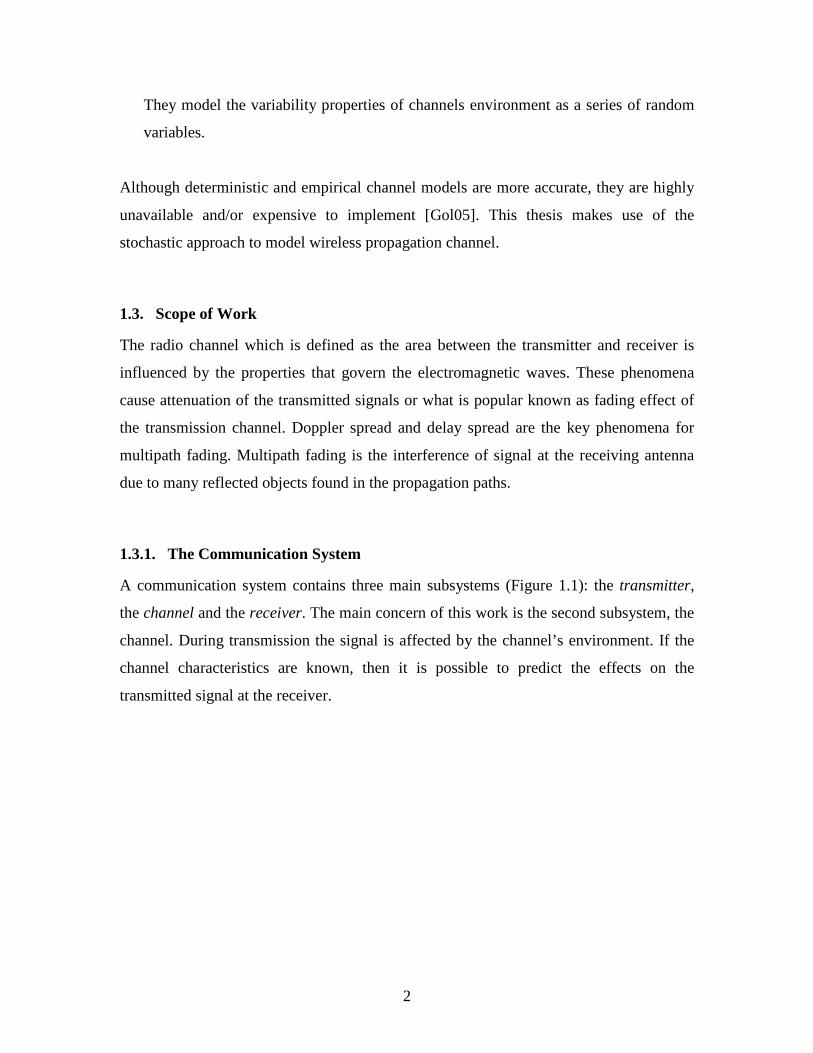
The properties of a radio propagation channel in a multipath fading environment can be
modeled from the analysis of the linear time varying radio channel as it gives an insight
of the physical properties that characterize the channel behavior such as scatterers and
reflectors that are found in the channel.
Receiver
Figure 2.1: Receiver in the presence of reflecting objects
5
Let the impulse response of the linear time varying multipath channel to be represented
by h(t, τ) and is described below as [Rap02]: -
( ) ( ) ( )( )( )
∑=
− −=tN
nn
tjn tetth n
0
),( ττδατ φ (2.1)
Where;
N(t) – the number of the multipath signal components present in the channel (at
time t)
τn(t) – the delay of the nth multipath signal component
αn(t) – the amplitude of the nth signal multipath component
φn(t) – the phase shift associated with the nth multipath component
The phase element, ( )tnφ contains the contributions from multipath delay, ( )tnτφ and
doppler shift, ( )tndφ of each multipath component and is denoted as:
( ) ( ) ( )tttnn dn φφφ τ += (2.2)
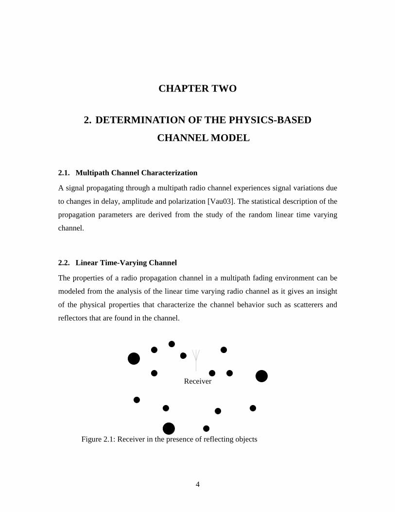
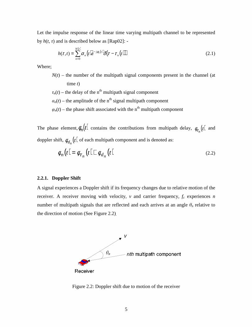
2.2.1. Doppler Shift
A signal experiences a Doppler shift if its frequency changes due to relative motion of the
receiver. A receiver moving with velocity, v and carrier frequency, fc experiences n
number of multipath signals that are reflected and each arrives at an angle θn relative to
the direction of motion (See Figure 2.2).
Figure 2.2: Doppler shift due to motion of the receiver

6
The doppler shift of the nth multipath component, ( )tfnd due to the receiver’s motion is
given by:
( ) ( )λθ tv
tfnd
cos= (2.3)
The receiver’s motion gives rise to phase shifts of each reflected multipath element. As a
result the signal amplitude varies randomly. The angle of arrival is assumed to be
uniformly distributed between [-π, π]. The phase shift associated with the Doppler
frequency is:
∫=t
nd dttfdn
)(2πφ (2.4)
2.2.2. Multipath Delay
Multipath delay, τn(t) is the measure of the time that the nth multipath signal takes to
arrive at the receiver. Delay for individual multipath component at the receiver is
calculated by using their corresponding path length, rn(t) and the speed of light, c.
c
trt n
n
)()( =τ (2.5)
The phase shift related to the delay is
( )tfjn
nce τπτφ 2−= (2.6)
2.2.3. The Field Strength Amplitude
Let the transmitting signal has a transmitting power Pt and gain Gt. The receiving signal
power Pr with gain Gr can be calculated using:
LGGPP rttr
1= (2.7)
The path loss, L is given by:
7
24
=λπd
L (2.8)
Where d is the free space distance in meters from transmitter to the receiver and λ is the
wavelength of the transmitted signal.
The power density, S (W/m2) at a distance d from the transmitting antenna is given by
24 d
GPS tt
π= (2.9)
The field strength of the receiving antenna, Er (V/m) is related to the power density by the
following formula:
π120
2
rES = (2.10)
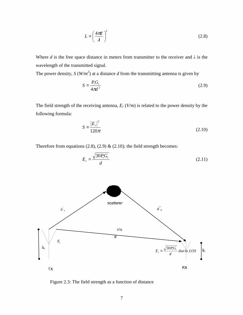
Therefore from equations (2.8), (2.9) & (2.10); the field strength becomes:
d
GPE tt
r
30= (2.11)
LOStodued
GPE tt
r
30=
tE
Figure 2.3: The field strength as a function of distance
8
If a signal is traveling and encounter an nth scattering object as shown in the above figure,
the field strength, En would be:
'''
30
nn
ttn dd
GPE
+Γ= (2.12)
Where:
• Γ – the reflection coefficient
• '''nn dandd are the distances traveled by signal before and after its
reflection from the nth reflecting object
Reflection coefficient conditions:
1. Depending on the encountered reflecting object, the reflection coefficient of the
reflecting objects ranges from 0 to 1
10 <Γ<⇒ (2.13)
2. Reflection coefficient Γ is related to the absorption coefficient Τ by:
122 =Τ+Γ (2.14)
Lower bound calculations of reflection coefficients of reflecting objects:
Assuming there is 50% absorption during the encounter of the signal with the reflecting
object, from equation (2.14) it follows that the lower bound of the reflection coefficient is
given as:
5.02 =Γ
707.0=Γ⇒ (2.15)
Combining equations (2.13) and (2.15) to determine the reflection coefficient range as:
0.707 < Γ< 1
Consequently;
d
GP
dd
GP tt
nn
tt 3030'''
≤+
Γ (2.16)
9
This implies at the receiver, maximum field strength, Er-max;
d
GPE tt
r
30max =−
(2.17)
Equation (2.17) is equivalent to equation (2.11) and it describes the field strength due to
LOS line.
2.3. Development of the Physics-based channel Model
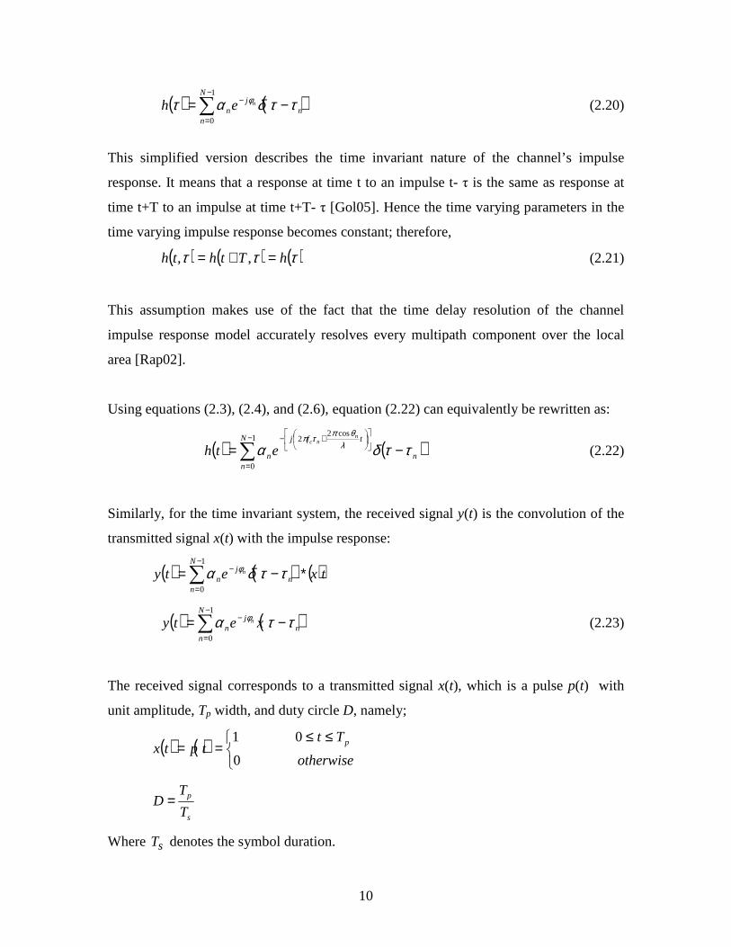
The received signal y(t) is the convolution of the transmitted signal x(t) and the time
varying impulse response, h(t, τ). By definition, this means: -
( ) ( ) ( )∫∞
∞−−= τττ dthtxty ,
( ) ( ) ( )ττ ,* thxty = (2.18)
( )τ,th
Figure 2.4: Impulse response The equation (2.1) describes the impulse response h(t, τ), hence the received signal from
equation (2.18) becomes:
( ) ( ) ( )( )( )
∑=
− −=tN
nn
tjn txetty n
0
)( ττα φ (2.19)
If the channel is time invariant or can be characterized as having wide sense stationarity
over a small scale distance or over a short-time interval, then the channel impulse
response has the complex form defined as:
10
( ) ( )∑−
=
− −=1
0
N
nn
jn
neh ττδατ φ (2.20)
This simplified version describes the time invariant nature of the channel’s impulse
response. It means that a response at time t to an impulse t- τ is the same as response at
time t+T to an impulse at time t+T- τ [Gol05]. Hence the time varying parameters in the
time varying impulse response becomes constant; therefore,
( ) ( ) ( )τττ hTthth =+= ,, (2.21)
This assumption makes use of the fact that the time delay resolution of the channel
impulse response model accurately resolves every multipath component over the local
area [Rap02].
Using equations (2.3), (2.4), and (2.6), equation (2.22) can equivalently be rewritten as:
( ) ( )n
tfjN
nn
nnc
eth ττδα λθπτπ
−=
+−−
=∑
cos221
0
(2.22)
Similarly, for the time invariant system, the received signal y(t) is the convolution of the
transmitted signal x(t) with the impulse response:
( ) ( ) ( )txetyN
nn
jn
n ∗−=∑−
=
−1
0
ττδα φ
( ) ( )∑−
=
− −=1
0
N
nn
jn xety n ττα φ (2.23)
The received signal corresponds to a transmitted signal x(t), which is a pulse p(t) with
unit amplitude, Tp width, and duty circle D, namely;
( ) ( ) ≤≤
==otherwise
Tttptx
p
0
01
s
p
T
TD =
Where sT denotes the symbol duration.
11
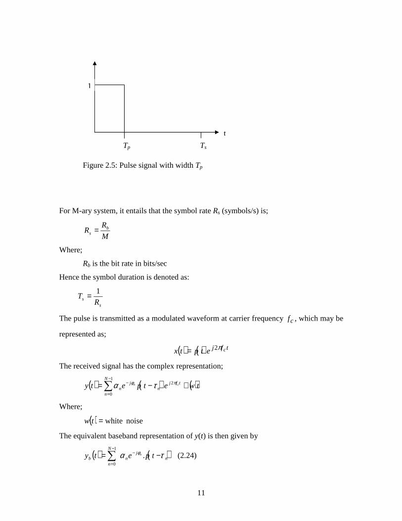
Figure 2.5: Pulse signal with width Tp
For M-ary system, it entails that the symbol rate Rs (symbols/s) is;
M
RR b
s =
Where;
Rb is the bit rate in bits/sec
Hence the symbol duration is denoted as:
ss R
T1=
The pulse is transmitted as a modulated waveform at carrier frequency cf , which may be
represented as;
( ) ( ) tfj cetptx π2=
The received signal has the complex representation;
( ) ( ) ( )twetpety tfjN
nn
jn
cn +−=∑−
=
− πφ τα 21
0
Where;
( ) noise white=tw
The equivalent baseband representation of y(t) is then given by
( ) ( )nj
n
N
nb tpety n τα φ −= −
−
=∑ .
1
0
(2.24)
1
Tp
t
Ts
12
The received signal can be further derived as follows: -
( ) ( )
−= ∑−
=
− tfjN
nn
jn
cn etpety πφ τα 21
0
.Re
( ) ( ) ( )
−⋅−⋅
−= ∑−
=tfjtftpjty ccn
N
nnnnn ππτφαφα 2cos2coscoscosRe
1
0
( )
( )n
N
n
N
ncnncnn
N
ncnn
N
ncnn
tptftfj
tfjtfty
τπφαπφα
πφαπφα
−⋅
+−
+=
∑ ∑
∑∑
−
=
−
=
−
=
−
=
1
0
1
0
1
0
1
0
2sinsin2cossin
2sincos2coscosRe
( )
( )n
N
ncnn
N
ncnn
N
ncnn
N
ncnn
tptftfj
tftfty
τπφαπφα
πφαπφα
−⋅
−+
+=
∑∑
∑∑
−
=
−
=
−
=
−
=
1
0
1
0
1
0
1
0
2cossin2sincos
2sinsin2coscosRe
( ) ( ) ( ) tftptftpty c
xComponentQuadrature
N
nnnnc
xcomponentinphase
N
nnnn
QI
πτφαπτφα 2sinsin2coscos
,
1
0
,
1
0
⋅−⋅+⋅−⋅= ∑∑−
=
−
= 444 3444 21444 3444 21
( ) ( )
( ) ( )∑
∑−
=
−
=
−⋅=
−⋅=⇒
1
0
1
0
sin component, quadrature theand
cos component, inphase The
N
nnnnQ
N
nnnnI
tpty
tpty
τφα
τφα
The envelope of the received signal is described as:
( ) ( ) ( )txtxta QIr22 += (2.25)
2.4. The Simulation Model
Let the transmitted signal, x(t) with bandwidth Bu and carrier frequency fc, be represented
by a pulse whose width is Tp as follows;
( ) ( ){ }tfj cetptx π2Re= (13)
Where;
13
( ) ≤≤
=otherwise
Tttp
p
0
01
p(t) is the equivalent lowpass signal of x(t).
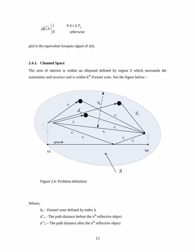
2.4.1. Channel Space
The area of interest is within an ellipsoid defined by region S which surrounds the
transmitter and receiver and is within kth Fresnel zone. See the figure below: -
''nd''
3d
''1d
''2d
'nd
'1d
'2d
'3d
iE
rE
kh
S
0d
Figure 2.6: Problem definition Where;
hk – Fresnel zone defined by index k
d’n – The path distance before the nth reflective object
d’’ n – The path distance after the nth reflective object
14
d0– Distance between transmitter and receiver
Ei – Incident signal’s field strength
Er – Reflected signal’s field strength
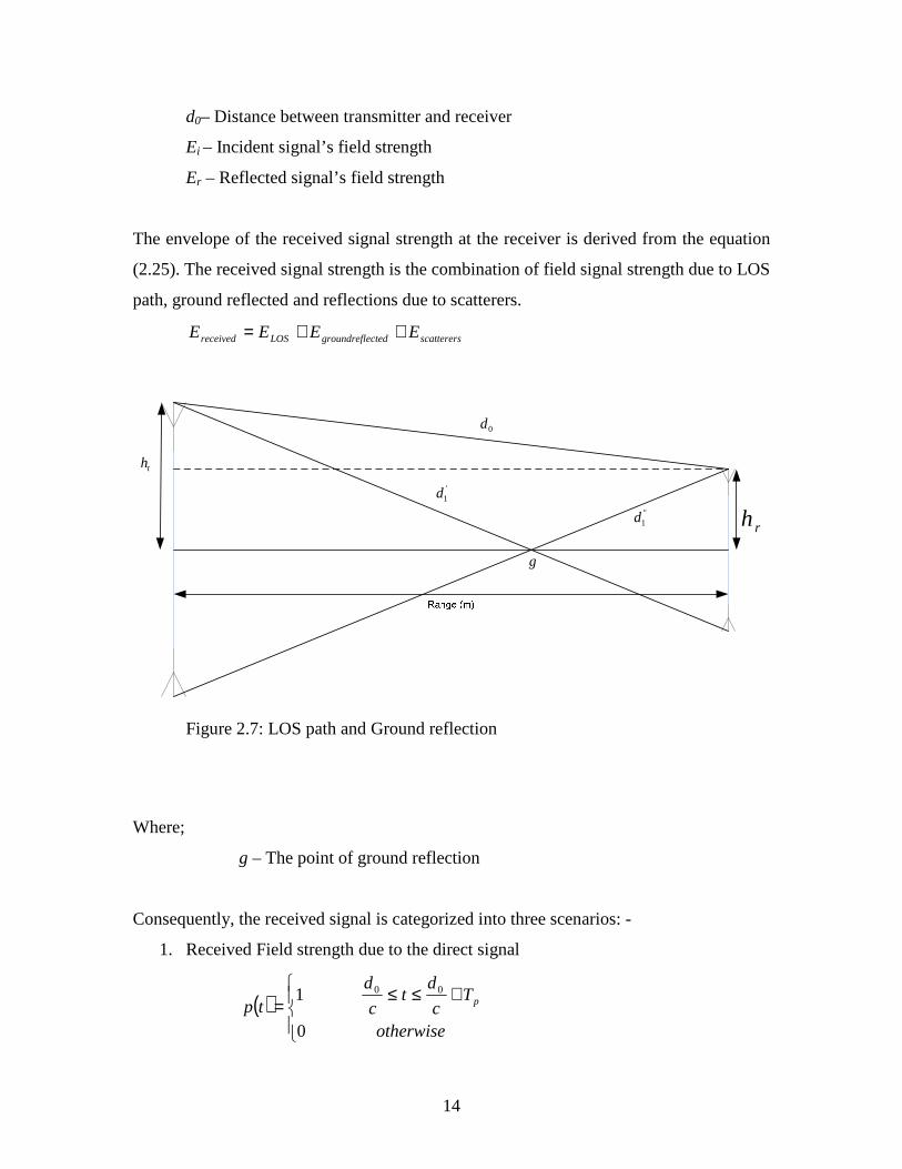
The envelope of the received signal strength at the receiver is derived from the equation
(2.25). The received signal strength is the combination of field signal strength due to LOS
path, ground reflected and reflections due to scatterers.
scatterersectedgroundreflLOSreceived EEEE ++=
''1d
'1d
th
rh
0d
g
Figure 2.7: LOS path and Ground reflection
Where;
g – The point of ground reflection
Consequently, the received signal is categorized into three scenarios: -
1. Received Field strength due to the direct signal
( )
+≤≤=
otherwise
Tc
dt
c
dtp p
0
1 00
15
Factors of equation (2.24) are defined as;
Amplitude, α0: 0
0
30
d
GP tt=α
Delay, τ0 : c
d00 =τ
Doppler frequency, 0df :
λθπ 0cos2
0
vf d =
2. Received Field strength due to ground reflection with reflection coefficient, Γg
( )
+
+≤≤
+=
otherwise
Tc
ddt
c
ddA
tp pp
0
2''
1'1
''1
'1
Similarly, factors of equation (2.24) for ground reflection scenario are defined as;
Amplitude, α1: ''1
'1
1
30
dd
GP ttg +
Γ=α
Delay, τ1 : c
dd ''1
'1
1
+=τ
Doppler frequency, 1df :
λθπ 1cos2
1
vfd =
3. Received Field strength due to reflection of multipath components from scatterers
( )
++≤≤+
=otherwise
Tc
ddt
c
ddA
tp pnnnn
p
0
2''''''
Likewise, factors of equation (2.24) for the reflecting objects are defined as;
Amplitude, αn: '''
30
nn
ttnn dd
GP
+Γ=α
16
Delay, τn : c
dd nnn
''' +=τ
Doppler frequency, ndf :
λθπ n
dv
fn
cos2=
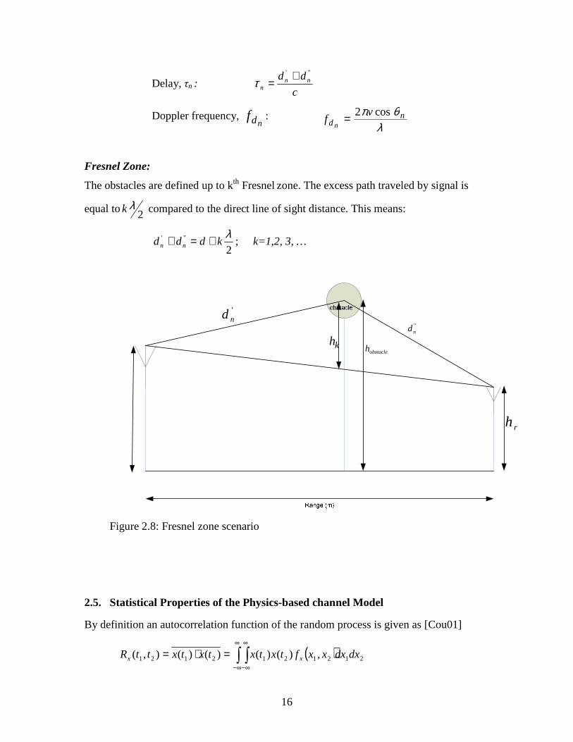
Fresnel Zone:
The obstacles are defined up to kth Fresnel zone. The excess path traveled by signal is
equal to 2λk compared to the direct line of sight distance. This means:
2''' λ
kddd nn +=+ ; k=1,2, 3, …
'nd
''nd
obstaclehkh
rh
Figure 2.8: Fresnel zone scenario
2.5. Statistical Properties of the Physics-based channel Model
By definition an autocorrelation function of the random process is given as [Cou01]
( ) 2121212121 ,)()()()(),( dxdxxxftxtxtxtxttR xx ∫ ∫∞
∞−
∞
∞−
=⋅=
17
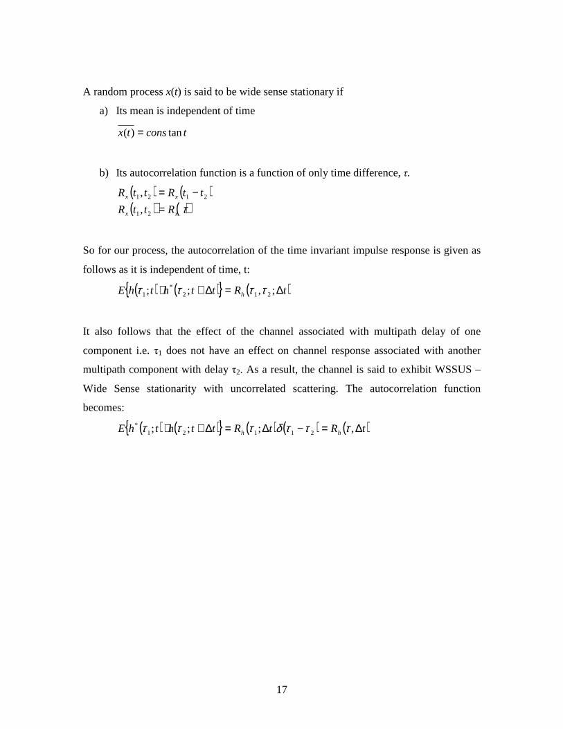
A random process x(t) is said to be wide sense stationary if
a) Its mean is independent of time
tconstx tan)( =
b) Its autocorrelation function is a function of only time difference, τ.
( ) ( )( ) ( )τxx
xx
RttR
ttRttR
=−=
21
2121
,
,
So for our process, the autocorrelation of the time invariant impulse response is given as
follows as it is independent of time, t:
( ) ( ){ } ( )tRtththE h ∆=∆+⋅ ;,;; 212*
1 ττττ
It also follows that the effect of the channel associated with multipath delay of one
component i.e. τ1 does not have an effect on channel response associated with another
multipath component with delay τ2. As a result, the channel is said to exhibit WSSUS –
Wide Sense stationarity with uncorrelated scattering. The autocorrelation function
becomes:
( ) ( ){ } ( ) ( ) ( )tRtRtththE hh ∆=−∆=∆+⋅ ,;;; 21121* τττδτττ
18
CHAPTER THREE
3. CHANNEL TYPE ASSESSMENT
As we have seen in the developed channel model; the received signal that has been
subjected to time varying channel, is the sum of amplitudes and time delays of the
multipath components that have arrived at the receiver at a particular time instance.
From the signal’s power delay profile, channel parameters such as mean excess delay,
RMS delay spread and excess delay spread are determined. Power delay profile shows
the signal’s strength and arrival time of each multipath component at the receiver. This
profile helps in determining the main parameters of multipath radio channel.
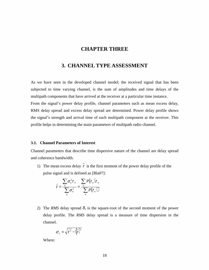
3.1. Channel Parameters of Interest
Channel parameters that describe time dispersive nature of the channel are delay spread
and coherence bandwidth.
1) The mean excess delay τ is the first moment of the power delay profile of the
pulse signal and is defined as [Bla07]:
( )( )∑
∑
∑
∑==
nn
nnn
nn
nnn
P
P
τ
ττ
α
τατ
2
2
2) The RMS delay spread δτ is the square-root of the second moment of the power
delay profile. The RMS delay spread is a measure of time dispersion in the
channel.
( )22 ττσ τ −=
Where:
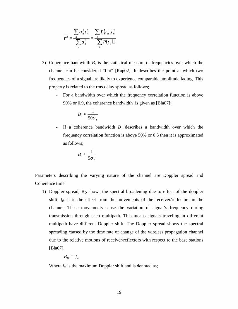
19
( )( )∑
∑
∑
∑==
nn
nnn
nn
nnn
P
P
τ
ττ
α
τατ
2
2
22
2
3) Coherence bandwidth Bc is the statistical measure of frequencies over which the
channel can be considered “flat” [Rap02]. It describes the point at which two
frequencies of a signal are likely to experience comparable amplitude fading. This
property is related to the rms delay spread as follows;
- For a bandwidth over which the frequency correlation function is above
90% or 0.9, the coherence bandwidth is given as [Bla07];
τσ50
1≈cB
- If a coherence bandwidth Bc describes a bandwidth over which the
frequency correlation function is above 50% or 0.5 then it is approximated
as follows;
τσ5
1≈cB
Parameters describing the varying nature of the channel are Doppler spread and
Coherence time.
1) Doppler spread, BD shows the spectral broadening due to effect of the doppler
shift, fd. It is the effect from the movements of the receiver/reflectors in the
channel. These movements cause the variation of signal’s frequency during
transmission through each multipath. This means signals traveling in different
multipath have different Doppler shift. The Doppler spread shows the spectral
spreading caused by the time rate of change of the wireless propagation channel
due to the relative motions of receiver/reflectors with respect to the base stations
[Bla07].
mD fB =
Where fm is the maximum Doppler shift and is denoted as;
20
λv
fm =
2) Coherence time Tc is inversely related to Doppler spread and is expressed as
follows;
mc f
T1≈
Coherence time is the statistical measure of the time duration over which the
channel impulse response is essentially invariant, and quantifies the similarity of
the channel response at different times [Rap02]. It describes the duration of time
at which two signals at the receiver experience possible amplitude correlation.
- If this coherence time is defined at the time over which the time
correlation function is over 50% or 0.5 then coherence time is denoted as:
mc f
Tπ16
9≈
As a rule of thumb, the coherence time is approximated as a geometric mean
of the two above equation.
mc f
T423.0≈
The analysis of multipath fading channel using these time and frequency dispersion
parameters help to evaluate type of wireless channel that is of concern.
3.2. Types of Multipath Fading in Wireless Channel
In assessing the type of fading that is being experienced in a channel during small scale
fading, the comparison between the nature of the transmitted signal and different channel
parameters need to be examined. The multipath wireless channels are categorized in four
different types; namely, Flat slow fading, Flat fast fading, Frequency-selective slow
fading and Frequency-selective fast fading. These categories stem from the two
independent propagation mechanisms; multipath delay spread and Doppler spread.
21
3.2.1. Effects of Fading as a Result of Time Dispersion of Multipath Channel
The time delay spread due to multipath results in flat or frequency selective channel.
Flat Fading:
A channel is said to convey a flat fading effect if it has a constant gain and linear phase
response over a bandwidth which is more than that of the transmitted signal [Gol02]. Flat
fading channel has its multipath time delay spread δτ much smaller than the transmitted
signal symbol duration Ts and the channels coherence bandwidth Bc is greater than the
transmitted signal’s bandwidth Bs. As a result, flat fading channel affects all frequency
components of a narrow band transmitted signal the same way and hence the signal will
experience the same magnitude of fading at the receiver.
Frequency-Selective Fading:
A wireless channel will reflect frequency-selective fading on the received signal if it has
a constant gain and linear phase response over a bandwidth which is less than the
transmitted signal’s bandwidth. This channel has multipath delay spread that is larger
than the transmitted signal’s symbol duration and its channel coherence bandwidth is
much smaller than the transmitted signal’s bandwidth. As a result, the Different
frequency components of the signal therefore experience decorrelated fading.
3.2.2. Effects of Fading as a Result of Doppler Spread
A transmitted signal changes as compared to the rate of change of the wireless channel. If
the rate of change of the channel’s impulse response is faster or slower compared to the
symbol duration; then the channel may be classified as to be a fast fading or slow fading
channel respectively. The Doppler spread shows this frequency dispersion characteristic
of the channel due to motion.
The motion of the receiver or surrounding objects compared to the properties of the
baseband signal determines how fast or slow the multipath channel will fade.
22
Slow fading
Slow fading occurs when the Doppler spread of the wireless channel is much less
compared to the baseband bandwidth of the transmitted signal and channel’s coherence
time is greater than the transmitted signal symbol duration.
Fast fading
When channel’s Doppler spread is more than baseband bandwidth of the transmitted
signal then the channel undergoes fast fading. This time channel’s coherence time is
smaller than the transmitted signal’s symbol duration.
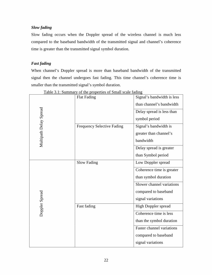
Table 3.1: Summary of the properties of Small scale fading Signal’s bandwidth is less
than channel’s bandwidth
Flat Fading
Delay spread is less than
symbol period
Signal’s bandwidth is
greater than channel’s
bandwidth
Mul
tipat
h D
elay
Spr
ead
Frequency Selective Fading
Delay spread is greater
than Symbol period
Low Doppler spread
Coherence time is greater
than symbol duration
Slow Fading
Slower channel variations
compared to baseband
signal variations
High Doppler spread
Coherence time is less
than the symbol duration
Dop
pler
Spr
ead
Fast fading
Faster channel variations
compared to baseband
signal variations
23
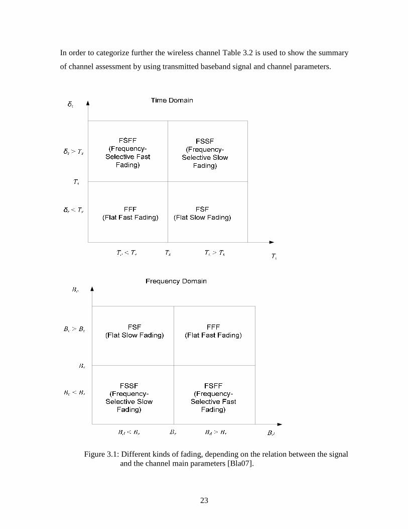
In order to categorize further the wireless channel Table 3.2 is used to show the summary
of channel assessment by using transmitted baseband signal and channel parameters.
Figure 3.1: Different kinds of fading, depending on the relation between the signal and the channel main parameters [Bla07].

24
CHAPTER FOUR
4. AUTOREGRESSIVE MODEL
Autoregressive model is of the form;
Figure 4.1: Autoregressive Model If p is the model order, an AR process is obtained by filtering white noise w(n) with an
all pole filter of the form [Hay96];
( ) ( ) [ ]nh
zazazazA
zHp
k
kk
pp
↔+
=+++
==
∑=
−∗−−
1
*1*1 1
1
...1
11
Where;
k = 1, 2,…, p
The above expressions are Yule-Walker equations and can be reproduced in matrix form
as follows;
][nx
( )zA
1
][nw
22εσσ =w
White Noise
Output Process
25
[ ] [ ] [ ] [ ][ ] [ ] [ ] [ ][ ] [ ] [ ] [ ]
[ ] [ ] [ ] [ ]
( )( )
( )
=
−−
−−
0
0
0
1
2
1
1
021
2012
1101
210
**
**
***
MM
L
MOMMM
L
L
L
p
p
p
p
xxxx
xxxx
xxxx
xxxx
pa
a
a
RpRpRpR
pRRRR
pRRRR
pRRRR
ε (4.1)
Equivalently it can be written as;
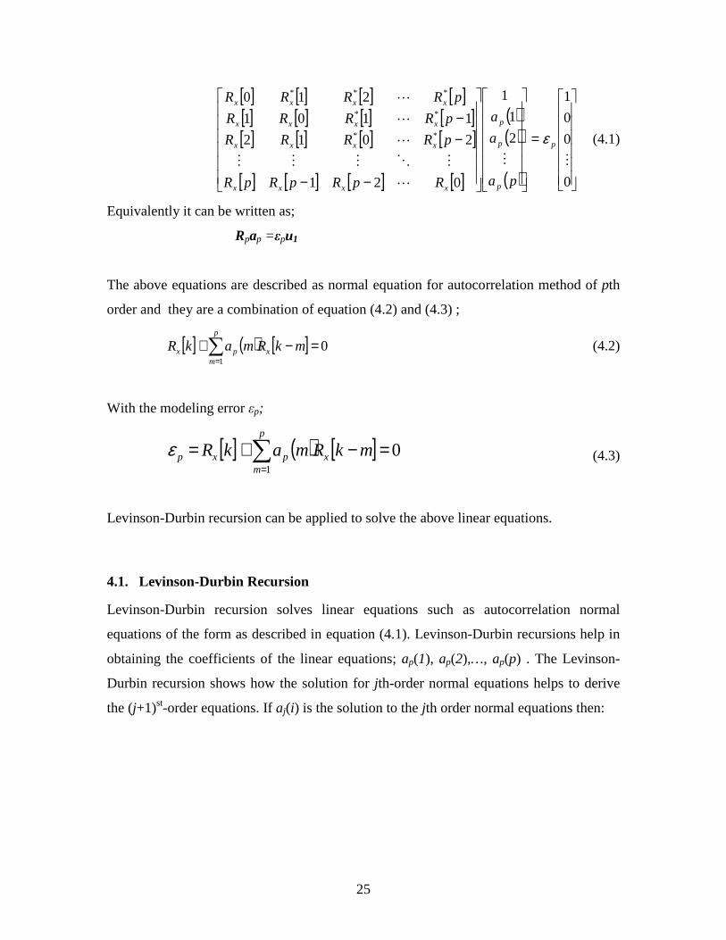
Rpap =εpu1
The above equations are described as normal equation for autocorrelation method of pth
order and they are a combination of equation (4.2) and (4.3) ;
[ ] ( ) [ ]∑=
=−+p
mxpx mkRmakR
1
0 (4.2)
With the modeling error εp;
[ ] ( ) [ ]∑=
=−+=p
mxpxp mkRmakR
1
0ε (4.3)
Levinson-Durbin recursion can be applied to solve the above linear equations.
4.1. Levinson-Durbin Recursion
Levinson-Durbin recursion solves linear equations such as autocorrelation normal
equations of the form as described in equation (4.1). Levinson-Durbin recursions help in
obtaining the coefficients of the linear equations; ap(1), ap(2),…, ap(p) . The Levinson-
Durbin recursion shows how the solution for jth-order normal equations helps to derive
the (j+1)st-order equations. If aj(i) is the solution to the jth order normal equations then:
26
[ ] [ ] [ ] [ ][ ] [ ] [ ] [ ][ ] [ ] [ ] [ ]
[ ] [ ] [ ] [ ]
( )( )
( )
=
−−
−−
0
0
0
2
1
1
021
2012
1101
210
**
**
***
MM
L
MOMMM
L
L
L j
j
j
j
xxxx
xxxx
xxxx
xxxx
ja
a
a
RjRjRjR
jRRRR
jRRRR
jRRRR ε
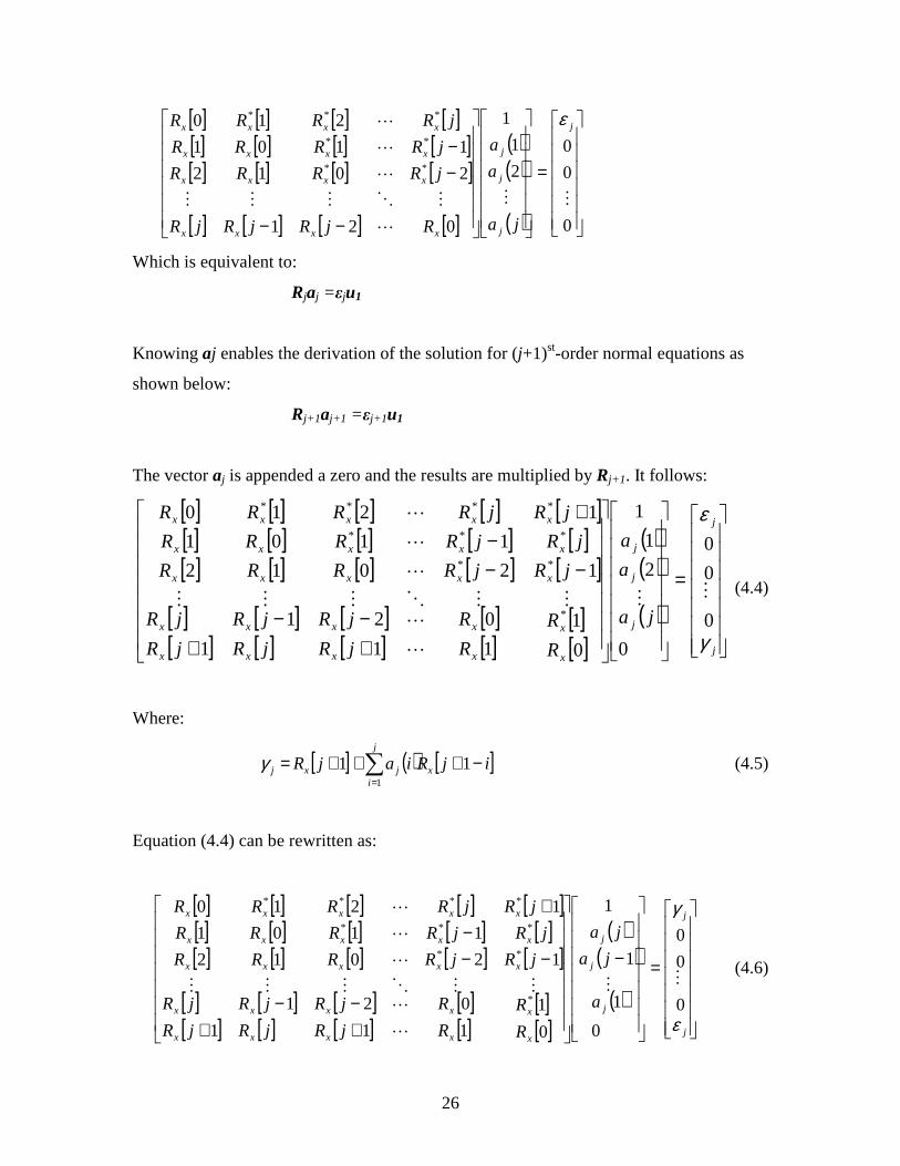
Which is equivalent to:
Rjaj =εju1
Knowing aj enables the derivation of the solution for (j+1)st-order normal equations as
shown below:
Rj+1aj+1 =εj+1u1
The vector aj is appended a zero and the results are multiplied by Rj+1. It follows:
[ ] [ ] [ ] [ ] [ ][ ] [ ] [ ] [ ] [ ][ ] [ ] [ ] [ ] [ ]
[ ][ ]
[ ][ ]
[ ][ ]
[ ][ ]
[ ][ ]
( )( )
( )
=
+−−
+
−−−
+
j
j
j
j
j
x
x
x
x
x
x
x
x
x
x
xxxxx
xxxxx
xxxxx
ja
a
a
R
R
R
R
jR
jR
jR
jR
jR
jR
jRjRRRR
jRjRRRR
jRjRRRR
γ
ε
0
0
0
0
2
1
1
0
1
1
0
1
21
1
12012
1101
1210
*
**
***
****
MM
L
LMMOMMM
L
L
L
(4.4)
Where:
[ ] ( ) [ ]∑=
−+++=j
ixjxj ijRiajR
1
11γ (4.5)
Equation (4.4) can be rewritten as:
[ ] [ ] [ ] [ ] [ ][ ] [ ] [ ] [ ] [ ][ ] [ ] [ ] [ ] [ ]
[ ][ ]
[ ][ ]
[ ][ ]
[ ][ ]
[ ][ ]
( )( )
( )
=
−
+−−
+
−−−
+
j
j
j
j
j
x
x
x
x
x
x
x
x
x
x
xxxxx
xxxxx
xxxxx
a
ja
ja
R
R
R
R
jR
jR
jR
jR
jR
jR
jRjRRRR
jRjRRRR
jRjRRRR
ε
γ
0
0
0
0
1
1
1
0
1
1
0
1
21
1
12012
1101
1210
*
**
***
****
MM
L
LMMOMMM
L
L
L
(4.6)
27
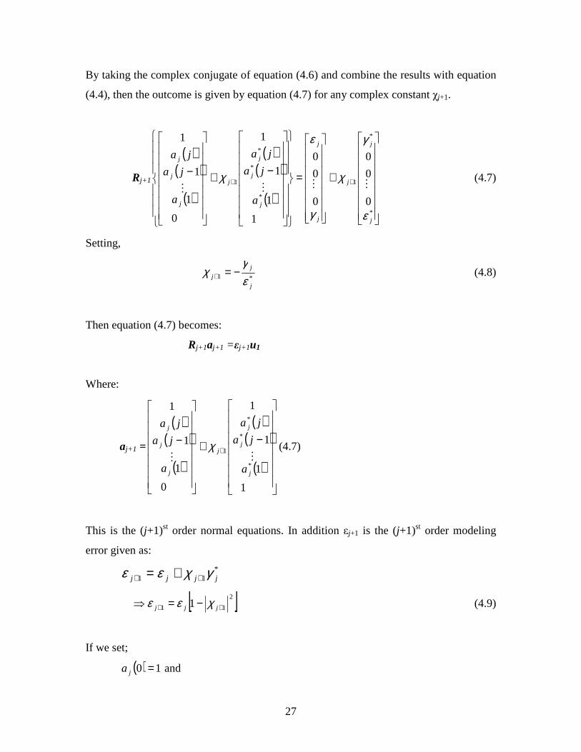
By taking the complex conjugate of equation (4.6) and combine the results with equation
(4.4), then the outcome is given by equation (4.7) for any complex constant χj+1.
Rj+1
( )( )
( )
( )( )
( )
+
=
−+
−++
*
*
1
*
*
*
1
0
0
0
0
0
0
1
1
1
1
0
1
1
1
j
j
j
j
j
j
j
j
j
j
j
j
a
ja
ja
a
ja
ja
ε
γ
χ
γ
ε
χMMMM
(4.7)
Setting,
*1
j
jj ε
γχ −=+ (4.8)
Then equation (4.7) becomes:
Rj+1aj+1 =εj+1u1
Where:
aj+1 =
( )( )
( )
( )( )
( )
−+
−+
1
1
1
1
0
1
1
1
*
*
*
1
j
j
j
j
j
j
j
a
ja
ja
a
ja
ja
MMχ (4.7)
This is the (j+1)st order normal equations. In addition εj+1 is the (j+1)st order modeling
error given as:
*11 jjjj γχεε ++ +=
[ ]2
11 1 ++ −=⇒ jjj χεε (4.9)
If we set;
( ) 10 =ja and
28
( ) 011 =++ ja j
Then;
( ) ( ) ( )1*11 +−+= ++ ijajaia jjjj χ
For i=0,1,…,j+1
4.1.1. Steps to Solve Normal Equations for Autocorrelation Method
In order to solve normal equations using the Levinson-Durbin recursion the following
steps need to be considered when using the Levinson-Durbin recursion [Hay96]:
1. The conditions to initiate the Levinson-Durbin recursion are defined using the
solution for the model of order j=0. Hence:
( ) 100 =a
( )00 xR=ε
2. For j=0, 1, …, p -1; the (j+1)st order model is determined using jth order model.
Using the equations below to determine the complex constant χj+1.
[ ] ( ) [ ]∑=
−+++=j
ixjxj ijRiajR
1
11γ
*1j
jj ε
γχ −=+
Then the recursion is updated to determine a j+1(i) from a j(i).
( ) ( ) ( )1*11 +−Γ+= ++ ijajaia jjjj
For i=1,2,..,j
( ) 11 1 ++ Γ=+ jj ja
3. The error εj+1 is then updated using:
[ ]2
11 1 ++ Γ−= jjj εε
The above equation can also be written as:
( ) ( ) ( )∑+
=++ +=
1
111 0
j
ixjxj iRiaRε
29
CHAPTER FIVE
5. COMPUTATION AND SIMULATION RESULTS
The physics-based channel model was simulated to generate data that depict the four
environment categories for wireless channel; Flat Fast Fading, Flat Slow Fading,
Frequency-Selective Fast Fading and Frequency-Selective Slow Fading. The parameters
for each category were examined to confirm the appropriate characteristics of each
environment.
For each scenario, autoregressive model was used to approximate the random channel
parameters generated by the channel models. Comparison was made of the two
autocorrelation functions generated from the data obtained from the physics-based
channel model, and the data obtained from the autoregressive process of each individual
wireless channel category. The two autocorrelation functions for each case describe: -
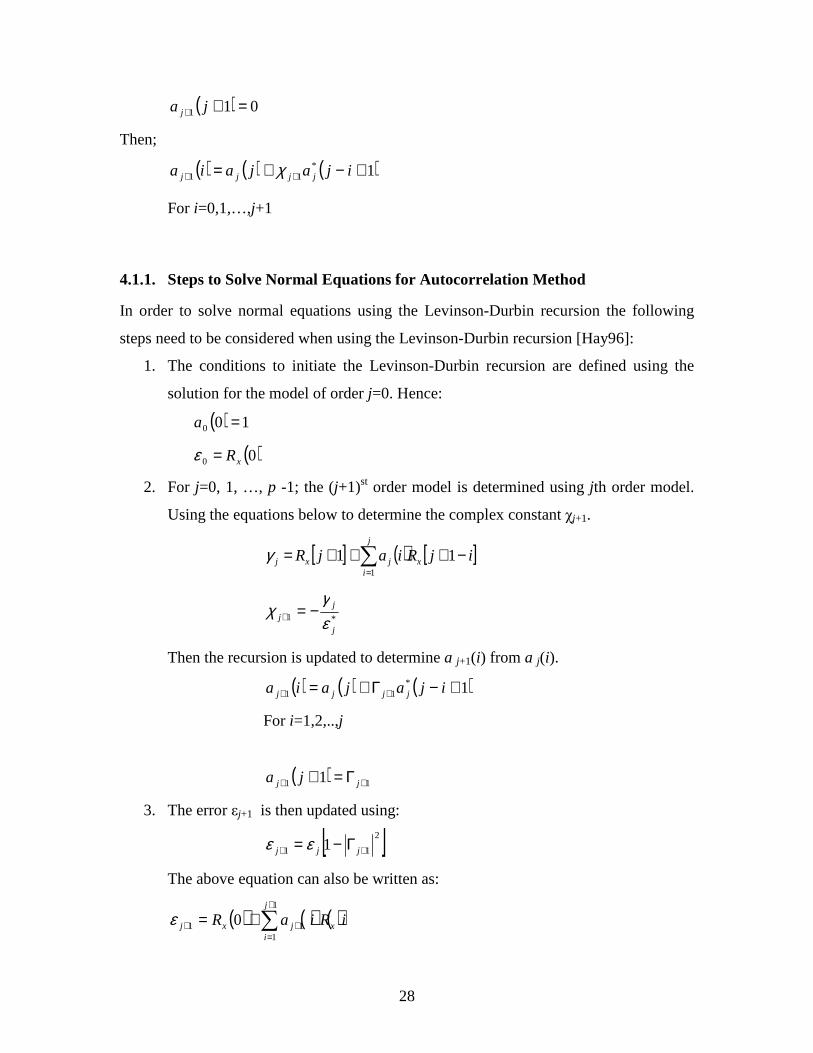
1. The output of the physics-based channel where p(t) is the input. The
autocorrelation function of the output, y(t) is Ry.
( )tp( )ty( )τ,th
Figure 5.1: Physics-based channel model
30
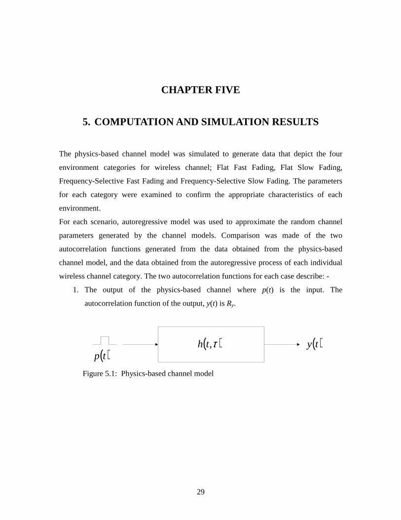
2. The output of the AR model after being driven by white noise, w[n]. The
autocorrelation function of the output x[n] is Rx.
( )zA
1[ ]nw [ ]nx
Figure 5.2: AR signal model Mean Square Error (MSE) was used to compare the two autocorrelation functions. MSE
is the cumulative squared error between autocorrelation obtained from the channel model
Ry to the one obtained form the AR process Rx. Mathematically, it is described as:
M
mRmR
MSE
M
m
yx
2
1
)()(
−
=∑
=
(5.1)
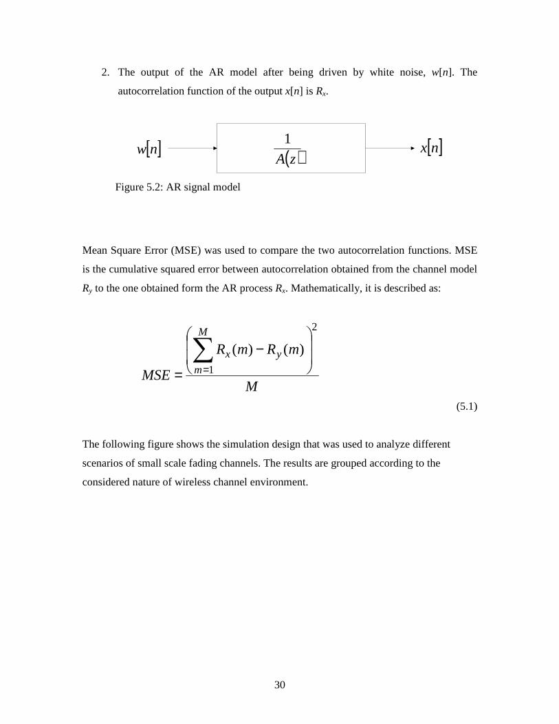
The following figure shows the simulation design that was used to analyze different
scenarios of small scale fading channels. The results are grouped according to the
considered nature of wireless channel environment.
31
Figure 5.3: Simulation Design
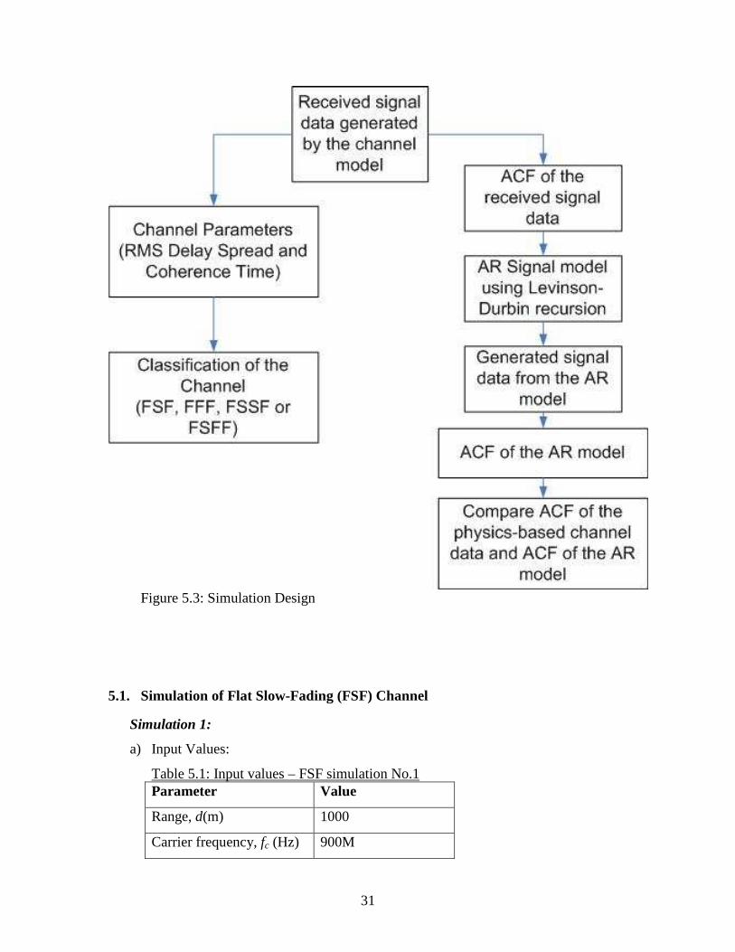
5.1. Simulation of Flat Slow-Fading (FSF) Channel
Simulation 1:
a) Input Values:
Table 5.1: Input values – FSF simulation No.1 Parameter Value
Range, d(m) 1000
Carrier frequency, fc (Hz) 900M
32
Parameter Value
Transmitter height, ht (m) 30
Receiver height, hr (m) 2
Vmax (m/s) 26
Number of obstacles, N 5
Data rate, Rb (bits/s) 1M
Fresnel zone, k=1e2
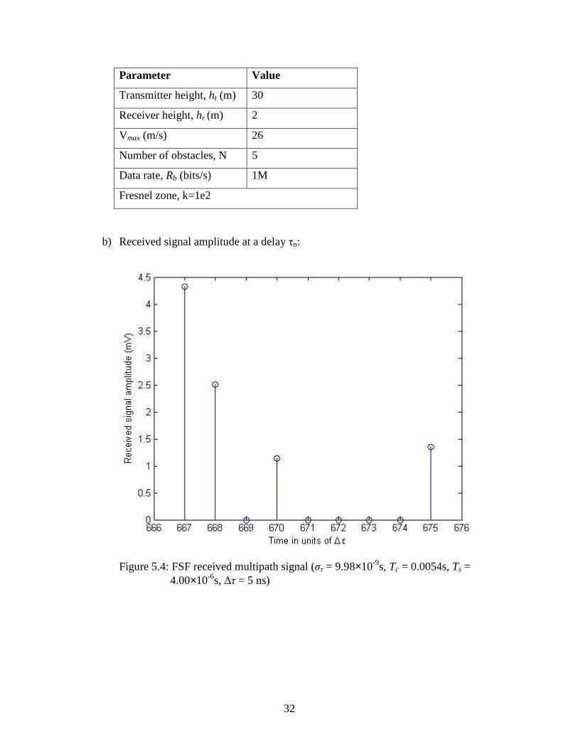
b) Received signal amplitude at a delay τn:
Figure 5.4: FSF received multipath signal (στ = 9.98×10⁻⁹s, Tc = 0.0054s, Ts = 4.00×10⁻⁶s, ∆τ = 5 ns)
33
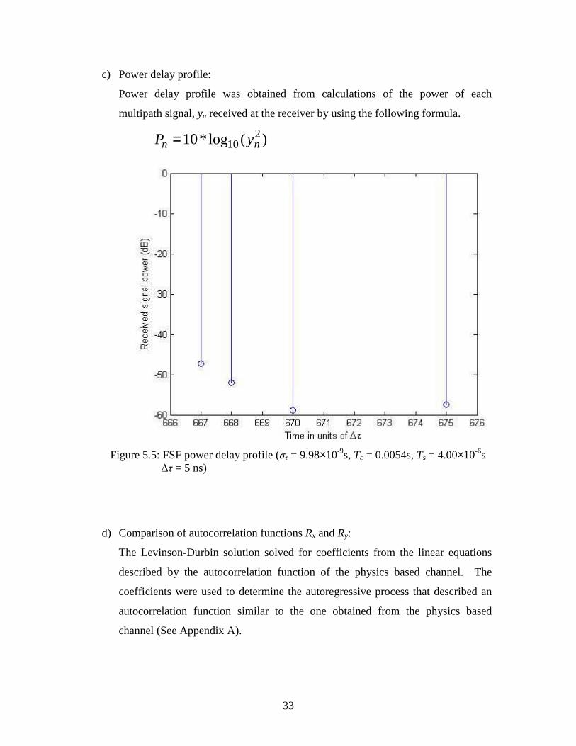
c) Power delay profile:
Power delay profile was obtained from calculations of the power of each
multipath signal, yn received at the receiver by using the following formula.
)(log*10 210 nn yP =
Figure 5.5: FSF power delay profile (στ = 9.98×10⁻⁹s, Tc = 0.0054s, Ts = 4.00×10⁻⁶s
∆τ = 5 ns)
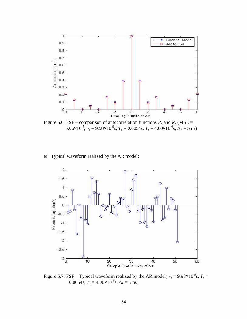
d) Comparison of autocorrelation functions Rx and Ry:
The Levinson-Durbin solution solved for coefficients from the linear equations
described by the autocorrelation function of the physics based channel. The
coefficients were used to determine the autoregressive process that described an
autocorrelation function similar to the one obtained from the physics based
channel (See Appendix A).
34
Figure 5.6: FSF – comparison of autocorrelation functions Rx and Rx (MSE =
5.06×10⁻⁵, στ = 9.98×10⁻⁹s, Tc = 0.0054s, Ts = 4.00×10⁻⁶s, ∆τ = 5 ns)
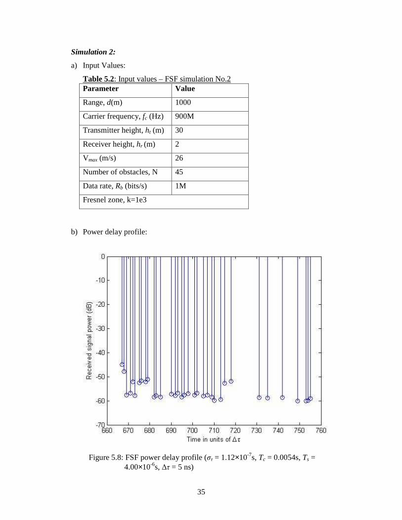
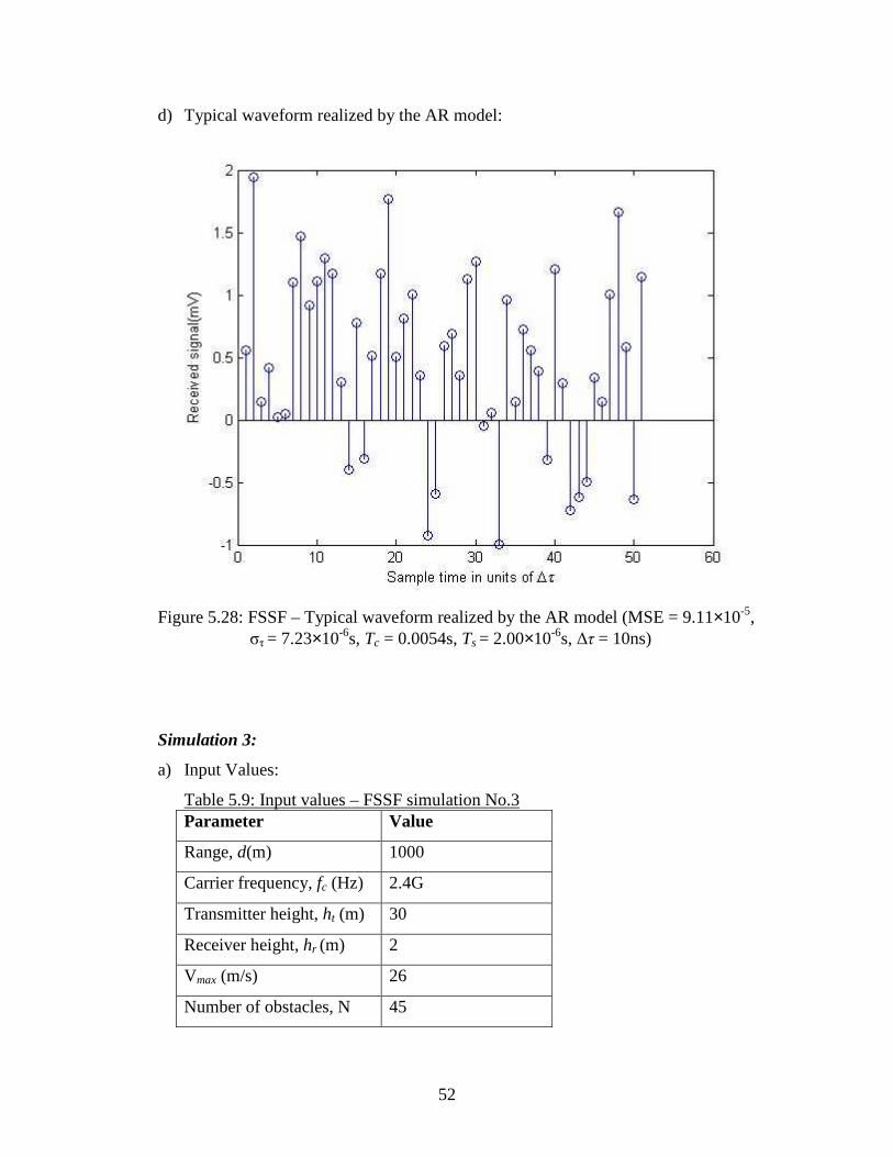
e) Typical waveform realized by the AR model:
Figure 5.7: FSF – Typical waveform realized by the AR model( στ = 9.98×10⁻⁹s, Tc = 0.0054s, Ts = 4.00×10⁻⁶s, ∆τ = 5 ns)
35
Simulation 2:
a) Input Values:
Table 5.2: Input values – FSF simulation No.2 Parameter Value
Range, d(m) 1000
Carrier frequency, fc (Hz) 900M
Transmitter height, ht (m) 30
Receiver height, hr (m) 2
Vmax (m/s) 26
Number of obstacles, N 45
Data rate, Rb (bits/s) 1M
Fresnel zone, k=1e3
b) Power delay profile:
Figure 5.8: FSF power delay profile (στ = 1.12×10⁻⁷s, Tc = 0.0054s, Ts = 4.00×10⁻⁶s, ∆τ = 5 ns)
36
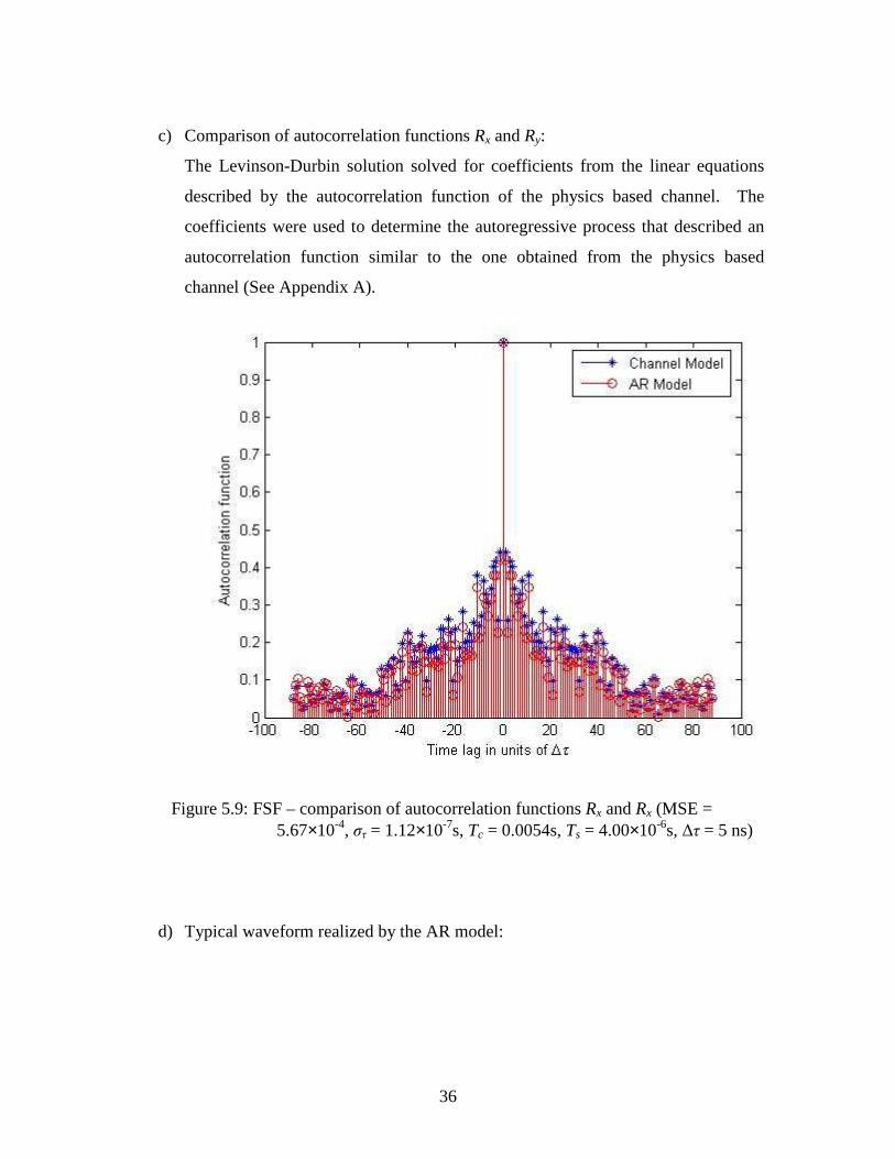
c) Comparison of autocorrelation functions Rx and Ry:
The Levinson-Durbin solution solved for coefficients from the linear equations
described by the autocorrelation function of the physics based channel. The
coefficients were used to determine the autoregressive process that described an
autocorrelation function similar to the one obtained from the physics based
channel (See Appendix A).
Figure 5.9: FSF – comparison of autocorrelation functions Rx and Rx (MSE =
5.67×10⁻⁴, στ = 1.12×10⁻⁷s, Tc = 0.0054s, Ts = 4.00×10⁻⁶s, ∆τ = 5 ns)
d) Typical waveform realized by the AR model:
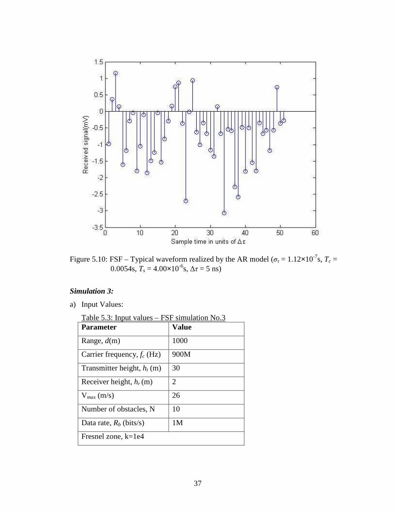
37
Figure 5.10: FSF – Typical waveform realized by the AR model (στ = 1.12×10⁻⁷s, Tc = 0.0054s, Ts = 4.00×10⁻⁶s, ∆τ = 5 ns)
Simulation 3:
a) Input Values:
Table 5.3: Input values – FSF simulation No.3 Parameter Value
Range, d(m) 1000
Carrier frequency, fc (Hz) 900M
Transmitter height, ht (m) 30
Receiver height, hr (m) 2
Vmax (m/s) 26
Number of obstacles, N 10
Data rate, Rb (bits/s) 1M
Fresnel zone, k=1e4
38
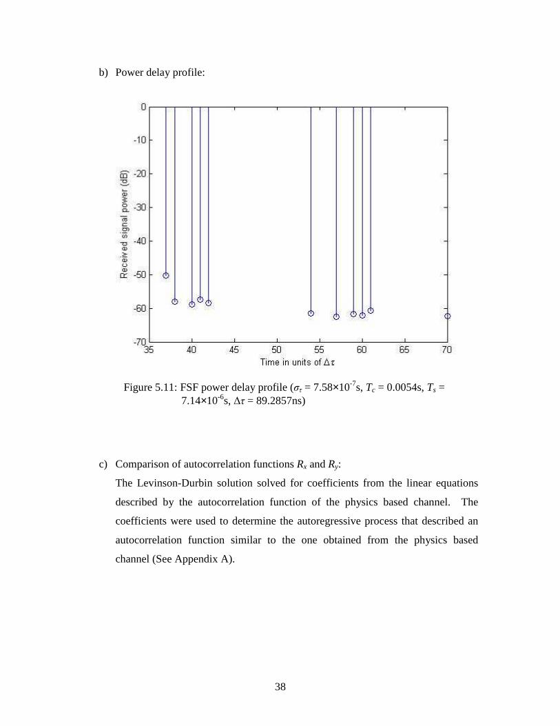
b) Power delay profile:
Figure 5.11: FSF power delay profile (στ = 7.58×10⁻⁷s, Tc = 0.0054s, Ts = 7.14×10⁻⁶s, ∆τ = 89.2857ns)
c) Comparison of autocorrelation functions Rx and Ry:
The Levinson-Durbin solution solved for coefficients from the linear equations
described by the autocorrelation function of the physics based channel. The
coefficients were used to determine the autoregressive process that described an
autocorrelation function similar to the one obtained from the physics based
channel (See Appendix A).
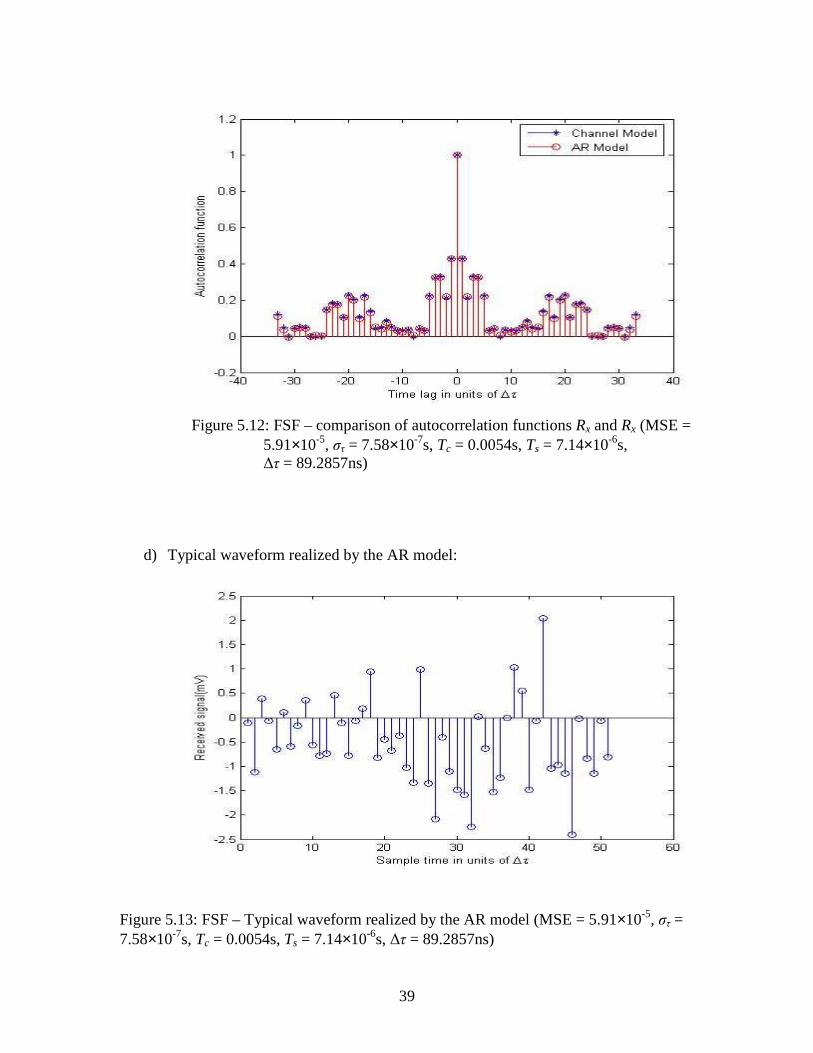
39
Figure 5.12: FSF – comparison of autocorrelation functions Rx and Rx (MSE = 5.91×10⁻⁵, στ = 7.58×10⁻⁷s, Tc = 0.0054s, Ts = 7.14×10⁻⁶s, ∆τ = 89.2857ns)
d) Typical waveform realized by the AR model:
Figure 5.13: FSF – Typical waveform realized by the AR model (MSE = 5.91×10⁻⁵, στ = 7.58×10⁻⁷s, Tc = 0.0054s, Ts = 7.14×10⁻⁶s, ∆τ = 89.2857ns)
40
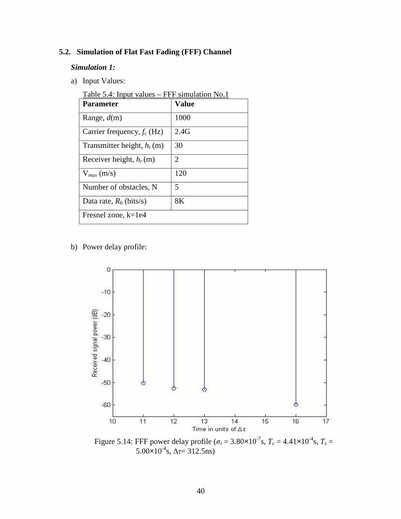
5.2. Simulation of Flat Fast Fading (FFF) Channel
Simulation 1:
a) Input Values:
Table 5.4: Input values – FFF simulation No.1 Parameter Value
Range, d(m) 1000
Carrier frequency, fc (Hz) 2.4G
Transmitter height, ht (m) 30
Receiver height, hr (m) 2
Vmax (m/s) 120
Number of obstacles, N 5
Data rate, Rb (bits/s) 8K
Fresnel zone, k=1e4
b) Power delay profile:
Figure 5.14: FFF power delay profile (στ = 3.80×10⁻⁷s, Tc = 4.41×10⁻⁴s, Ts =
5.00×10⁻⁴s, ∆τ= 312.5ns)
41
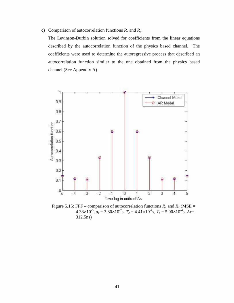
c) Comparison of autocorrelation functions Rx and Ry:
The Levinson-Durbin solution solved for coefficients from the linear equations
described by the autocorrelation function of the physics based channel. The
coefficients were used to determine the autoregressive process that described an
autocorrelation function similar to the one obtained from the physics based
channel (See Appendix A).
Figure 5.15: FFF – comparison of autocorrelation functions Rx and Rx (MSE =
4.33×10⁻⁵, στ = 3.80×10⁻⁷s, Tc = 4.41×10⁻⁴s, Ts = 5.00×10⁻⁴s, ∆τ= 312.5ns)
42
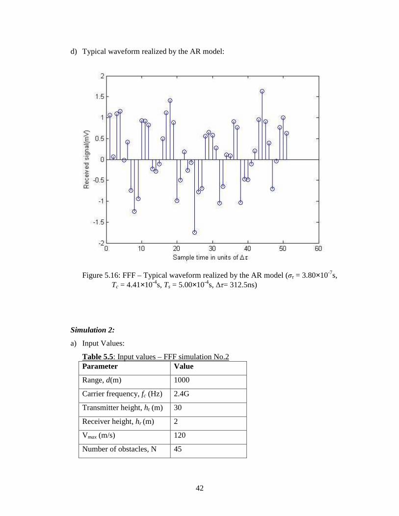
d) Typical waveform realized by the AR model:
Figure 5.16: FFF – Typical waveform realized by the AR model (στ = 3.80×10⁻⁷s, Tc = 4.41×10⁻⁴s, Ts = 5.00×10⁻⁴s, ∆τ= 312.5ns)
Simulation 2:
a) Input Values:
Table 5.5: Input values – FFF simulation No.2 Parameter Value
Range, d(m) 1000
Carrier frequency, fc (Hz) 2.4G
Transmitter height, ht (m) 30
Receiver height, hr (m) 2
Vmax (m/s) 120
Number of obstacles, N 45
43
Parameter Value
Data rate, Rb (bits/s) 8K
Fresnel zone, k=1e5
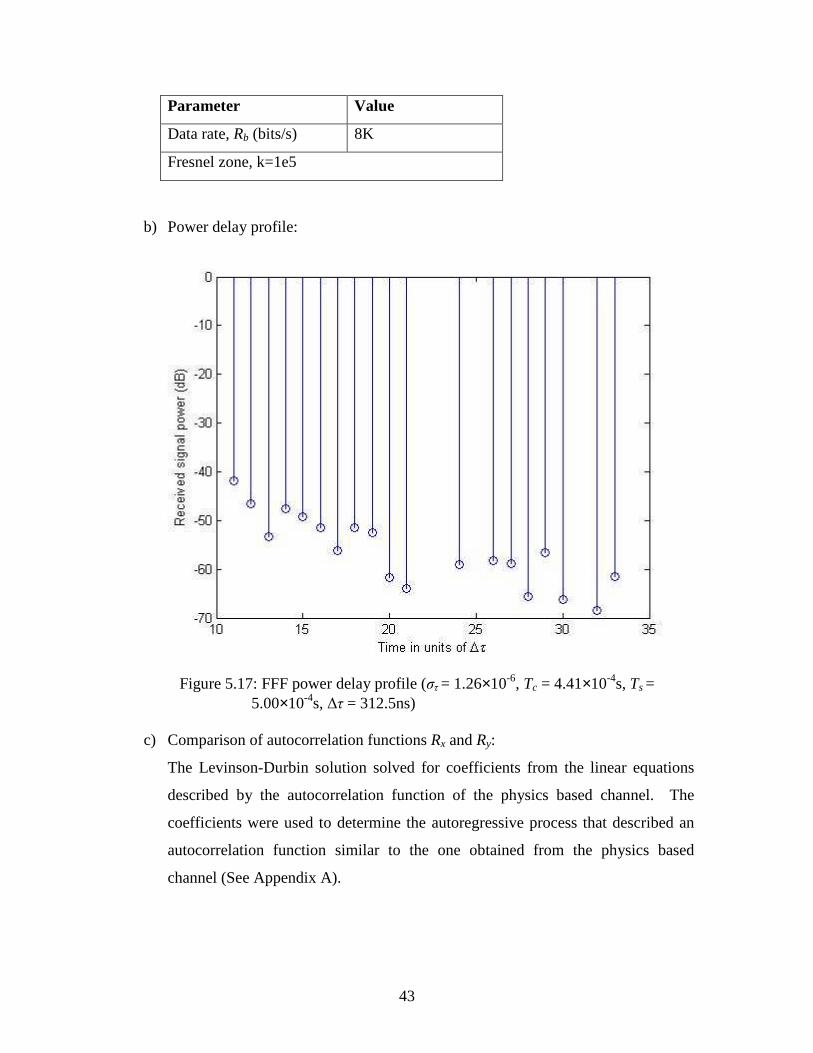
b) Power delay profile:
Figure 5.17: FFF power delay profile (στ = 1.26×10⁻⁶, Tc = 4.41×10⁻⁴s, Ts = 5.00×10⁻⁴s, ∆τ = 312.5ns)
c) Comparison of autocorrelation functions Rx and Ry:
The Levinson-Durbin solution solved for coefficients from the linear equations
described by the autocorrelation function of the physics based channel. The
coefficients were used to determine the autoregressive process that described an
autocorrelation function similar to the one obtained from the physics based
channel (See Appendix A).
44
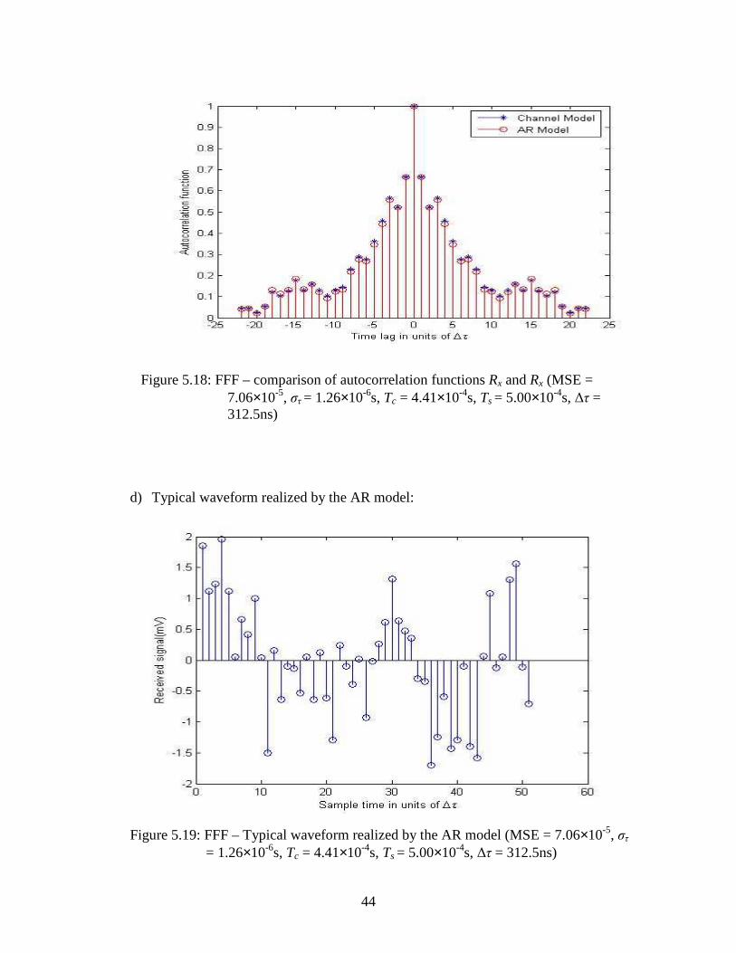
Figure 5.18: FFF – comparison of autocorrelation functions Rx and Rx (MSE =
7.06×10⁻⁵, στ = 1.26×10⁻⁶s, Tc = 4.41×10⁻⁴s, Ts = 5.00×10⁻⁴s, ∆τ = 312.5ns)
d) Typical waveform realized by the AR model:
Figure 5.19: FFF – Typical waveform realized by the AR model (MSE = 7.06×10⁻⁵, στ = 1.26×10⁻⁶s, Tc = 4.41×10⁻⁴s, Ts = 5.00×10⁻⁴s, ∆τ = 312.5ns)
45
Simulation 3:
a) Input Values:
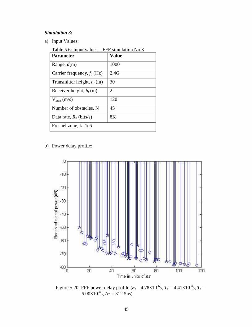
Table 5.6: Input values – FFF simulation No.3 Parameter Value
Range, d(m) 1000
Carrier frequency, fc (Hz) 2.4G
Transmitter height, ht (m) 30
Receiver height, hr (m) 2
Vmax (m/s) 120
Number of obstacles, N 45
Data rate, Rb (bits/s) 8K
Fresnel zone, k=1e6
b) Power delay profile:
Figure 5.20: FFF power delay profile (στ = 4.78×10⁻⁶s, Tc = 4.41×10⁻⁴s, Ts = 5.00×10⁻⁴s, ∆τ = 312.5ns)
46
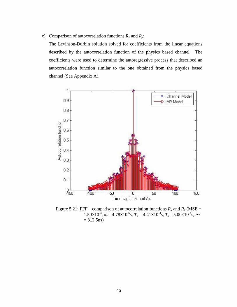
c) Comparison of autocorrelation functions Rx and Ry:
The Levinson-Durbin solution solved for coefficients from the linear equations
described by the autocorrelation function of the physics based channel. The
coefficients were used to determine the autoregressive process that described an
autocorrelation function similar to the one obtained from the physics based
channel (See Appendix A).
Figure 5.21: FFF – comparison of autocorrelation functions Rx and Rx (MSE = 1.50×10⁻⁴, στ = 4.78×10⁻⁶s, Tc = 4.41×10⁻⁴s, Ts = 5.00×10⁻⁴s, ∆τ = 312.5ns)
47
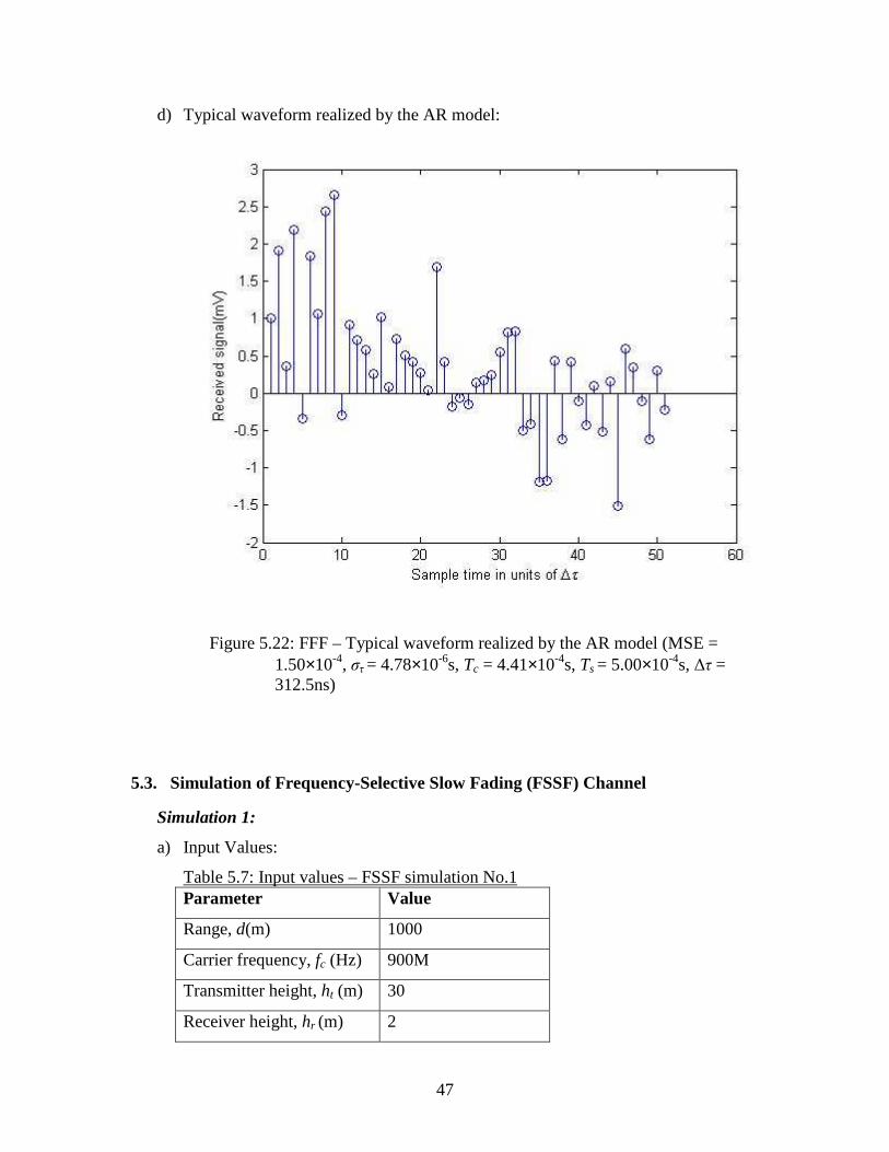
d) Typical waveform realized by the AR model:
Figure 5.22: FFF – Typical waveform realized by the AR model (MSE = 1.50×10⁻⁴, στ = 4.78×10⁻⁶s, Tc = 4.41×10⁻⁴s, Ts = 5.00×10⁻⁴s, ∆τ = 312.5ns)
5.3. Simulation of Frequency-Selective Slow Fading (FSSF) Channel
Simulation 1:
a) Input Values:
Table 5.7: Input values – FSSF simulation No.1 Parameter Value
Range, d(m) 1000
Carrier frequency, fc (Hz) 900M
Transmitter height, ht (m) 30
Receiver height, hr (m) 2
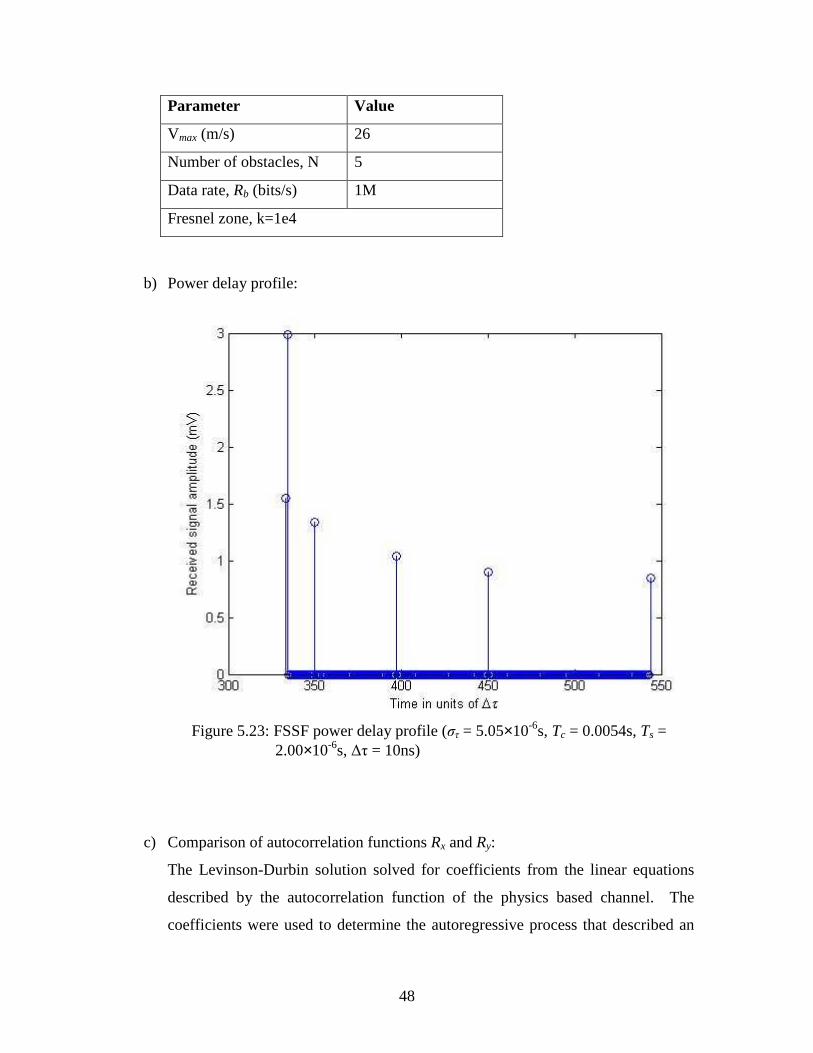
48
Parameter Value
Vmax (m/s) 26
Number of obstacles, N 5
Data rate, Rb (bits/s) 1M
Fresnel zone, k=1e4
b) Power delay profile:
Figure 5.23: FSSF power delay profile (στ = 5.05×10⁻⁶s, Tc = 0.0054s, Ts =
2.00×10⁻⁶s, ∆τ = 10ns)
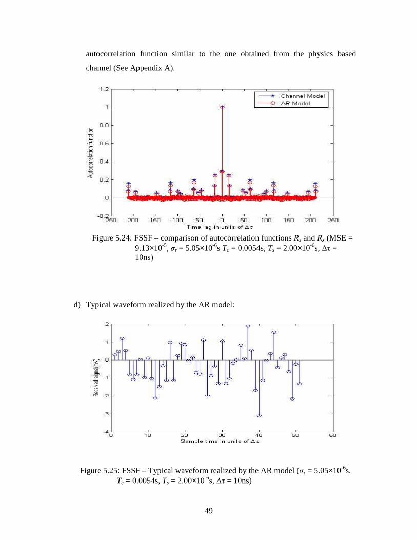
c) Comparison of autocorrelation functions Rx and Ry:
The Levinson-Durbin solution solved for coefficients from the linear equations
described by the autocorrelation function of the physics based channel. The
coefficients were used to determine the autoregressive process that described an
49
autocorrelation function similar to the one obtained from the physics based
channel (See Appendix A).
Figure 5.24: FSSF – comparison of autocorrelation functions Rx and Rx (MSE =
9.13×10⁻⁵, στ = 5.05×10⁻⁶s Tc = 0.0054s, Ts = 2.00×10⁻⁶s, ∆τ = 10ns)
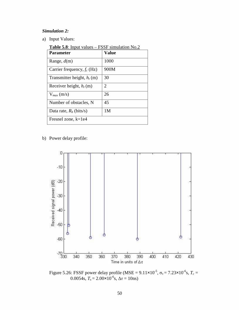
d) Typical waveform realized by the AR model:
Figure 5.25: FSSF – Typical waveform realized by the AR model (στ = 5.05×10⁻⁶s, Tc = 0.0054s, Ts = 2.00×10⁻⁶s, ∆τ = 10ns)
50
Simulation 2:
a) Input Values:
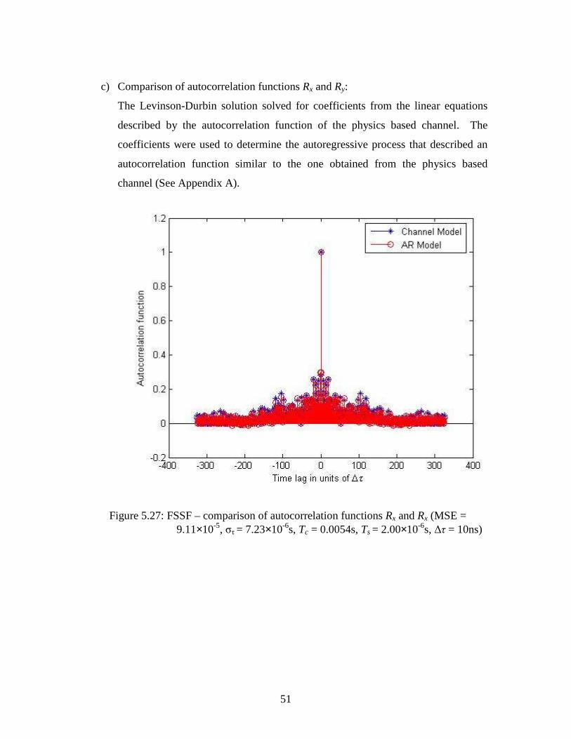
Table 5.8: Input values – FSSF simulation No.2 Parameter Value
Range, d(m) 1000
Carrier frequency, fc (Hz) 900M
Transmitter height, ht (m) 30
Receiver height, hr (m) 2
Vmax (m/s) 26
Number of obstacles, N 45
Data rate, Rb (bits/s) 1M
Fresnel zone, k=1e4
b) Power delay profile:
Figure 5.26: FSSF power delay profile (MSE = 9.11×10⁻⁵, στ = 7.23×10⁻⁶s, Tc = 0.0054s, Ts = 2.00×10⁻⁶s, ∆τ = 10ns)
51
c) Comparison of autocorrelation functions Rx and Ry:
The Levinson-Durbin solution solved for coefficients from the linear equations
described by the autocorrelation function of the physics based channel. The
coefficients were used to determine the autoregressive process that described an
autocorrelation function similar to the one obtained from the physics based
channel (See Appendix A).
Figure 5.27: FSSF – comparison of autocorrelation functions Rx and Rx (MSE =
9.11×10⁻⁵, στ = 7.23×10⁻⁶s, Tc = 0.0054s, Ts = 2.00×10⁻⁶s, ∆τ = 10ns)
52
d) Typical waveform realized by the AR model:
Figure 5.28: FSSF – Typical waveform realized by the AR model (MSE = 9.11×10⁻⁵, στ = 7.23×10⁻⁶s, Tc = 0.0054s, Ts = 2.00×10⁻⁶s, ∆τ = 10ns)
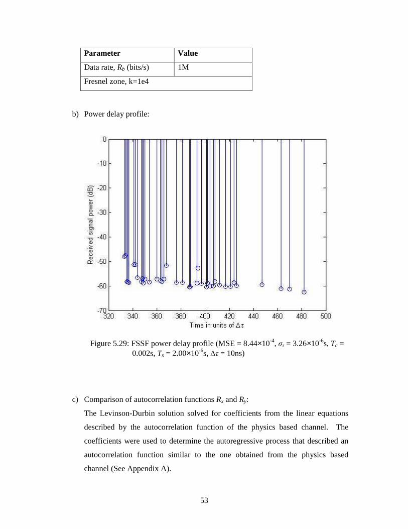
Simulation 3:
a) Input Values:
Table 5.9: Input values – FSSF simulation No.3 Parameter Value
Range, d(m) 1000
Carrier frequency, fc (Hz) 2.4G
Transmitter height, ht (m) 30
Receiver height, hr (m) 2
Vmax (m/s) 26
Number of obstacles, N 45
53
Parameter Value
Data rate, Rb (bits/s) 1M
Fresnel zone, k=1e4
b) Power delay profile:
Figure 5.29: FSSF power delay profile (MSE = 8.44×10⁻⁴, στ = 3.26×10⁻⁶s, Tc = 0.002s, Ts = 2.00×10⁻⁶s, ∆τ = 10ns)
c) Comparison of autocorrelation functions Rx and Ry:
The Levinson-Durbin solution solved for coefficients from the linear equations
described by the autocorrelation function of the physics based channel. The
coefficients were used to determine the autoregressive process that described an
autocorrelation function similar to the one obtained from the physics based
channel (See Appendix A).
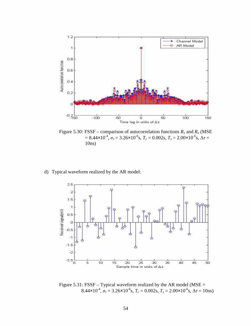
54
Figure 5.30: FSSF – comparison of autocorrelation functions Rx and Rx (MSE = 8.44×10⁻⁴, στ = 3.26×10⁻⁶s, Tc = 0.002s, Ts = 2.00×10⁻⁶s, ∆τ = 10ns)
d) Typical waveform realized by the AR model:
Figure 5.31: FSSF – Typical waveform realized by the AR model (MSE = 8.44×10⁻⁴, στ = 3.26×10⁻⁶s, Tc = 0.002s, Ts = 2.00×10⁻⁶s, ∆τ = 10ns)
55
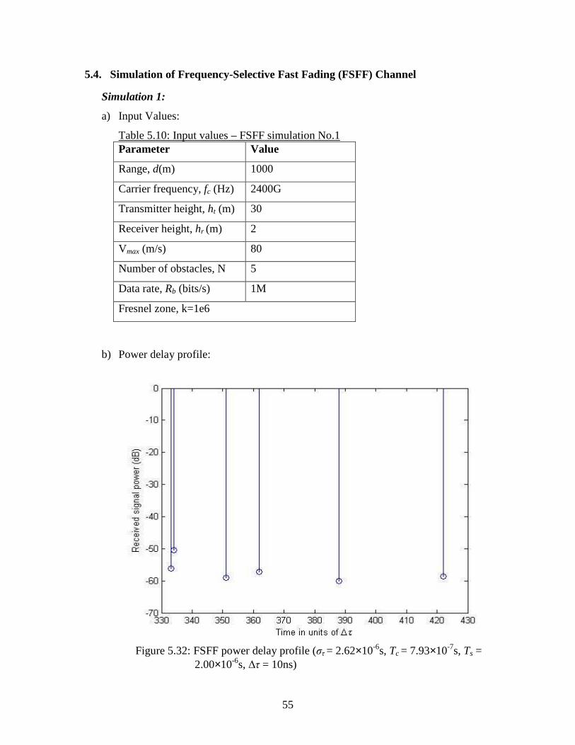
5.4. Simulation of Frequency-Selective Fast Fading (FSFF) Channel
Simulation 1:
a) Input Values:
Table 5.10: Input values – FSFF simulation No.1 Parameter Value
Range, d(m) 1000
Carrier frequency, fc (Hz) 2400G
Transmitter height, ht (m) 30
Receiver height, hr (m) 2
Vmax (m/s) 80
Number of obstacles, N 5
Data rate, Rb (bits/s) 1M
Fresnel zone, k=1e6
b) Power delay profile:
Figure 5.32: FSFF power delay profile (στ = 2.62×10⁻⁶s, Tc = 7.93×10⁻⁷s, Ts =
2.00×10⁻⁶s, ∆τ = 10ns)
56
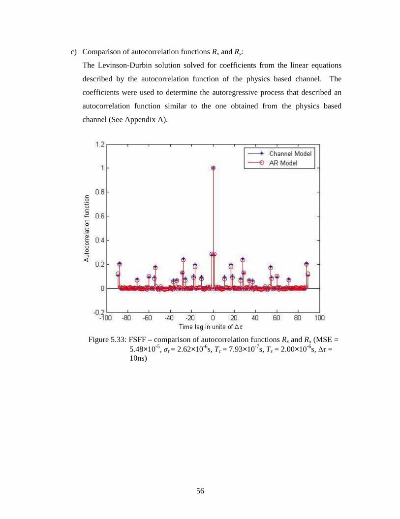
c) Comparison of autocorrelation functions Rx and Ry:
The Levinson-Durbin solution solved for coefficients from the linear equations
described by the autocorrelation function of the physics based channel. The
coefficients were used to determine the autoregressive process that described an
autocorrelation function similar to the one obtained from the physics based
channel (See Appendix A).
Figure 5.33: FSFF – comparison of autocorrelation functions Rx and Rx (MSE =
5.48×10⁻⁵, στ = 2.62×10⁻⁶s, Tc = 7.93×10⁻⁷s, Ts = 2.00×10⁻⁶s, ∆τ = 10ns)
57
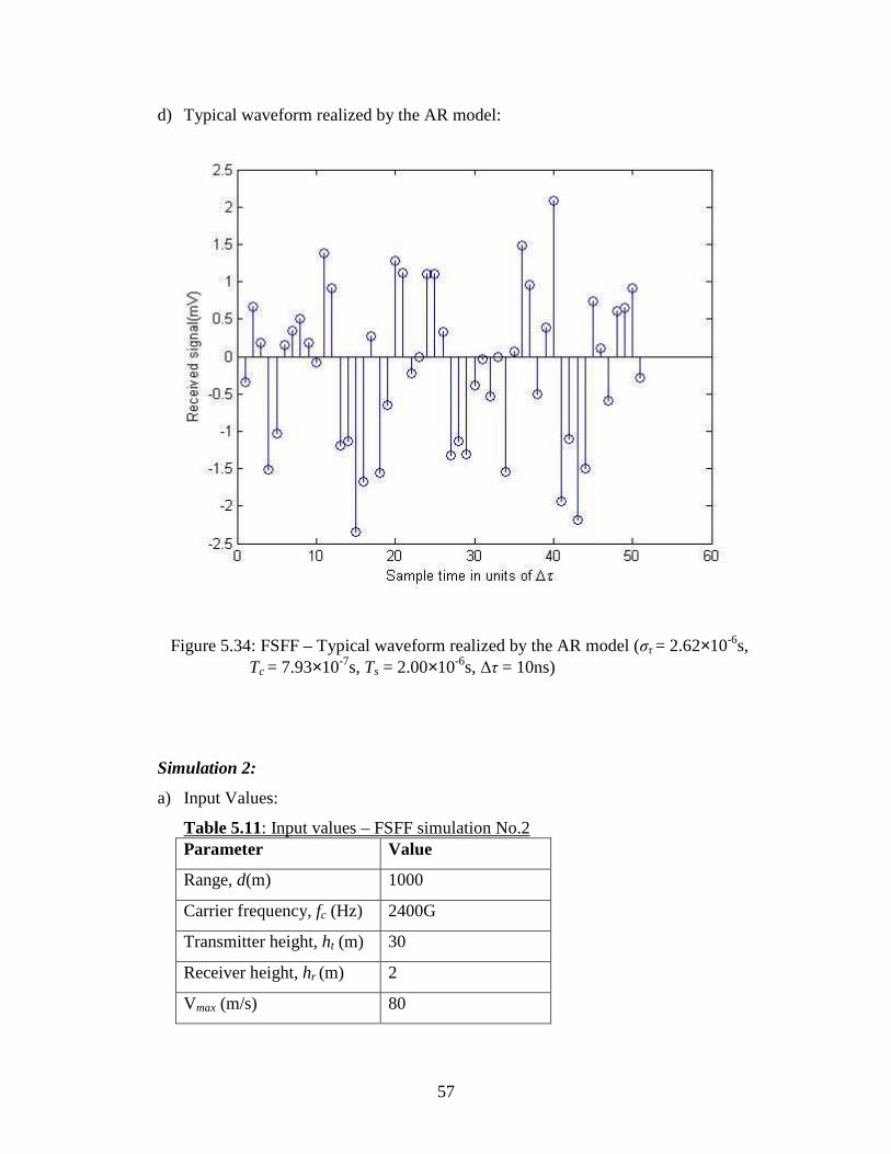
d) Typical waveform realized by the AR model:
Figure 5.34: FSFF – Typical waveform realized by the AR model (στ = 2.62×10⁻⁶s, Tc = 7.93×10⁻⁷s, Ts = 2.00×10⁻⁶s, ∆τ = 10ns)
Simulation 2:
a) Input Values:
Table 5.11: Input values – FSFF simulation No.2 Parameter Value
Range, d(m) 1000
Carrier frequency, fc (Hz) 2400G
Transmitter height, ht (m) 30
Receiver height, hr (m) 2
Vmax (m/s) 80
58
Parameter Value
Number of obstacles, N 45
Data rate, Rb (bits/s) 1M
Fresnel zone, k=1e6
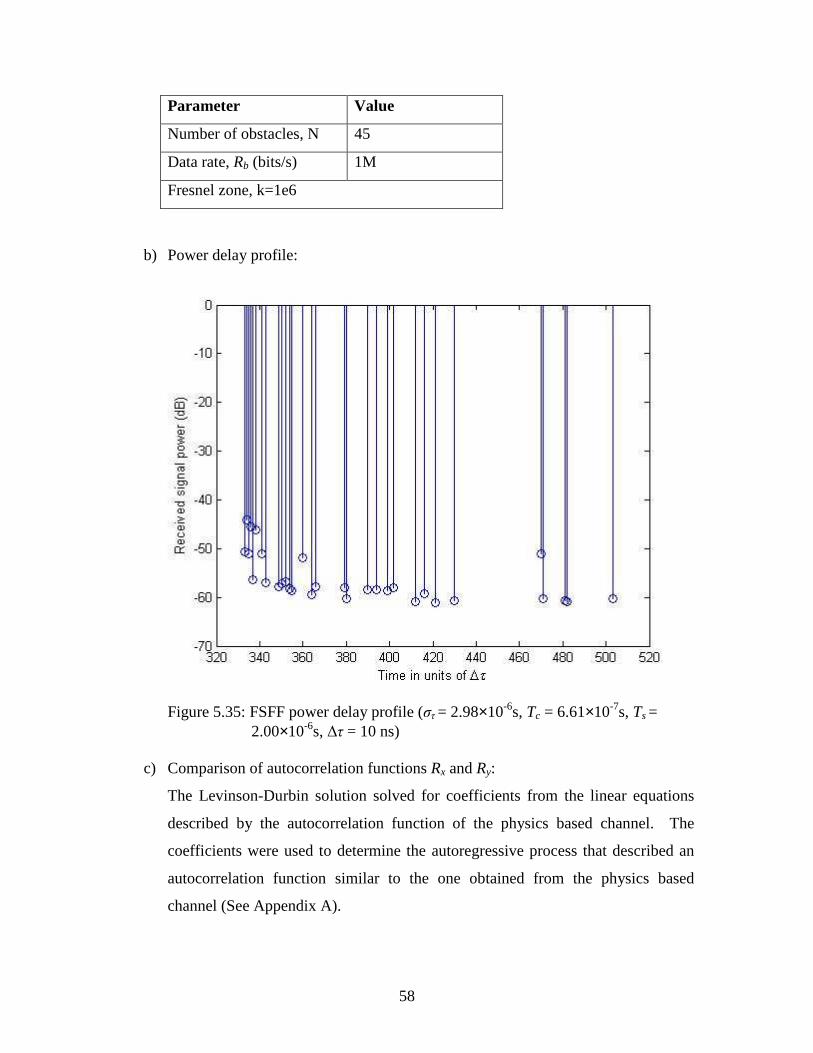
b) Power delay profile:
Figure 5.35: FSFF power delay profile (στ = 2.98×10⁻⁶s, Tc = 6.61×10⁻⁷s, Ts = 2.00×10⁻⁶s, ∆τ = 10 ns)
c) Comparison of autocorrelation functions Rx and Ry:
The Levinson-Durbin solution solved for coefficients from the linear equations
described by the autocorrelation function of the physics based channel. The
coefficients were used to determine the autoregressive process that described an
autocorrelation function similar to the one obtained from the physics based
channel (See Appendix A).
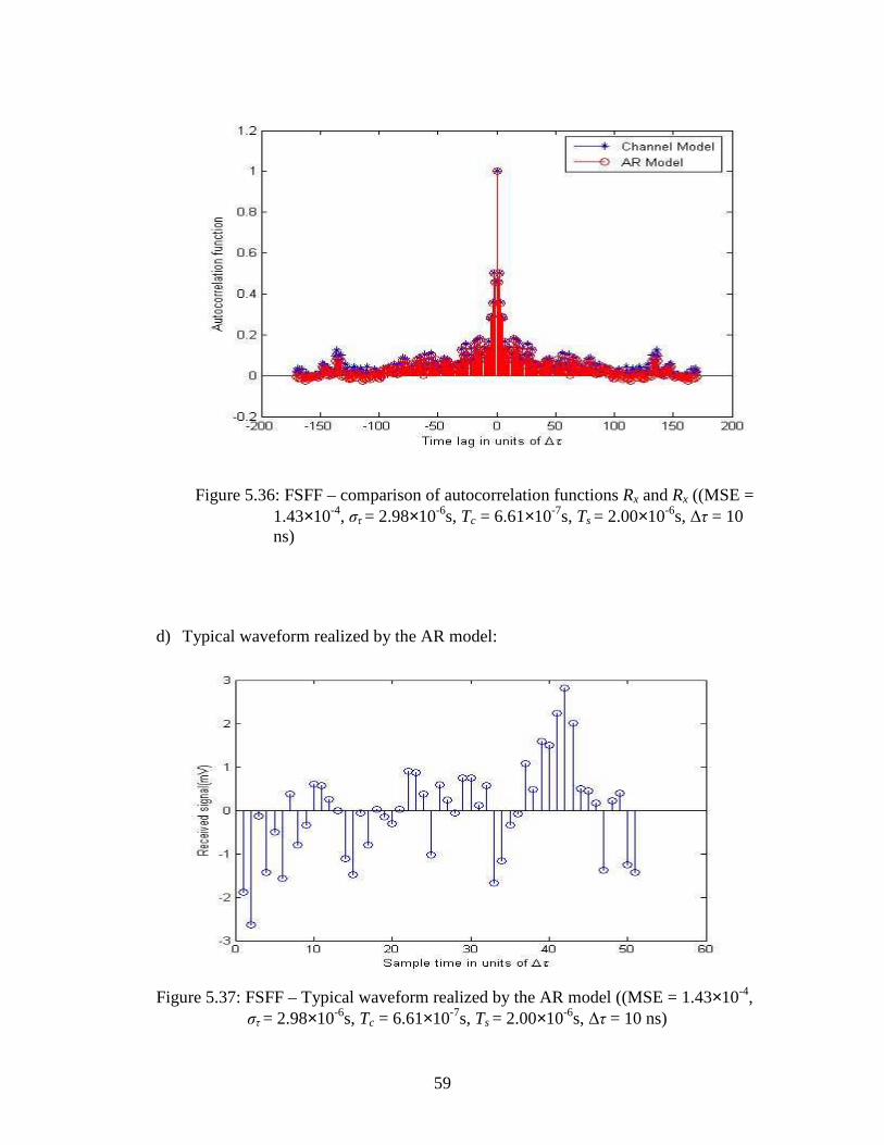
59
Figure 5.36: FSFF – comparison of autocorrelation functions Rx and Rx ((MSE =
1.43×10⁻⁴, στ = 2.98×10⁻⁶s, Tc = 6.61×10⁻⁷s, Ts = 2.00×10⁻⁶s, ∆τ = 10 ns)
d) Typical waveform realized by the AR model:
Figure 5.37: FSFF – Typical waveform realized by the AR model ((MSE = 1.43×10⁻⁴, στ = 2.98×10⁻⁶s, Tc = 6.61×10⁻⁷s, Ts = 2.00×10⁻⁶s, ∆τ = 10 ns)
60
CHAPTER SIX
6. CONCLUSION AND RECOMMENDATIONS
This research proposes a systematic procedure to simulate channel data in different
scenarios in small-scale fading environment. It was shown that the simulated channel
data from the physics-based model was then successfully estimated by an AR signal
model for different channel types. This procedure is an efficient way to generate inputs
for other channel estimation or tracking studies.
Typically, the channel data comes from the experimental measurements. However, these
practical measurements require some expensive devices such as transceivers and signal
processing boards. In addition, the information provided not only is it limited by
hardware but also it is bounded by geographic area. This proposed channel model
provides for cost-effective way of generating channel data. The modeling technique used
for this work can facilitates the design of optimal receivers such as that of MIMO
systems.
Recommendations and Future work:
1. Different channel type categories were realized (Flat Slow Fading, Flat Fast
Fading, Frequency-selective Slow Fading and Frequency-selective Fast Fading
channels); however the inputs used to categorize FSFF according to the definition
described in chapter four were not practical. For instance the carrier frequency
was in the order of 10-12. Additional work needs to be done to take into account
the practical realization of FSFF category of channel classification.
2. More work needs to be done to understand how the spatial distribution of
scattering objects and their velocities affect the channel characteristics, namely
the coherence time and RMS delay spread.
3. Finding ways to minimize the order p of the AR model.
61
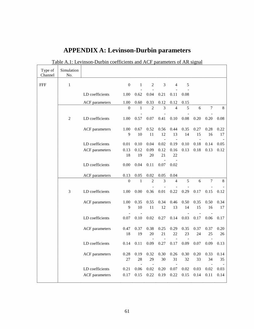
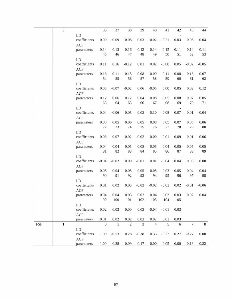
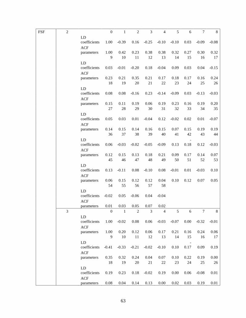
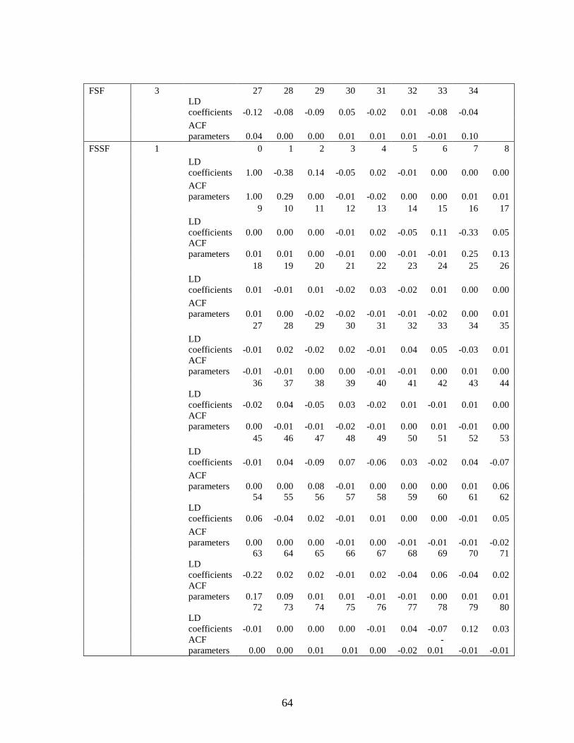
APPENDIX A: Levinson-Durbin parameters
Table A.1: Levinson-Durbin coefficients and ACF parameters of AR signal
Type of Channel
Simulation No.
FFF 1 0 1 2 3 4 5
LD coefficients 1.00 -
0.62 -
0.04 0.21 -
0.11 -
0.08
ACF parameters 1.00 0.60 0.33 0.12 0.12 0.15 0 1 2 3 4 5 6 7 8
2 LD coefficients 1.00 -
0.57 0.07 -
0.41 0.10 -
0.08 0.20 -
0.20 0.08
ACF parameters 1.00 0.67 0.52 0.56 0.44 0.35 0.27 0.28 0.22 9 10 11 12 13 14 15 16 17
LD coefficients 0.01 0.10 0.04 -
0.02 -
0.19 0.10 -
0.18 0.14 -
0.05
ACF parameters 0.13 0.12 0.09 0.12 0.16 0.13 0.18 0.13 0.12 18 19 20 21 22
LD coefficients 0.00 0.04 0.11 -
0.07 -
0.02
ACF parameters 0.13 0.05 0.02 0.05 0.04 0 1 2 3 4 5 6 7 8
3 LD coefficients 1.00 0.00 -
0.36 -
0.01 -
0.22 -
0.29 0.17 -
0.15 -
0.12
ACF parameters 1.00 0.35 0.55 0.34 0.46 0.50 0.35 0.50 0.34 9 10 11 12 13 14 15 16 17
LD coefficients -
0.07 -
0.10 0.02 0.27 0.14 -
0.03 -
0.17 -
0.06 0.17
ACF parameters 0.47 0.37 0.38 0.25 0.29 0.35 0.37 0.37 0.20 18 19 20 21 22 23 24 25 26
LD coefficients 0.14 0.11 -
0.09 -
0.27 -
0.17 -
0.09 0.07 -
0.09 0.13
ACF parameters 0.28 0.19 0.32 0.30 0.26 0.30 0.20 0.33 0.14 27 28 29 30 31 32 33 34 35
LD coefficients 0.21 -
0.06 -
0.02 0.20 -
0.07 0.02 0.03 -
0.02 -
0.03
ACF parameters 0.17 0.15 0.22 0.19 0.22 0.15 0.14 0.11 0.14
62
3 36 37 38 39 40 41 42 43 44
LD coefficients 0.09 -0.09 -0.08 0.03 -0.02 -0.21
-0.03 0.06 0.04
ACF parameters 0.14 0.13 0.16 0.12 0.14 0.15 0.11 0.14 0.11
45 46 47 48 49 50 51 52 53
LD coefficients 0.11 0.16 -0.12 0.01 0.02 -0.08 0.05 -0.02 -0.05
ACF parameters 0.16 0.11 0.15 0.08 0.09 0.11 0.08 0.13 0.07
54 55 56 57 58 59 60 61 62
LD coefficients 0.03 -0.07 -0.02 0.06 -0.05 0.00 0.05 0.02 0.12
ACF parameters 0.12 0.06 0.12 0.04 0.08 0.05 0.08 0.07 0.05
63 64 65 66 67 68 69 70 71
LD coefficients 0.04 -0.06 0.05 0.03 -0.10 -0.05
-0.07 0.01 -0.04
ACF parameters 0.08 0.05 0.06 0.05 0.08 0.05 0.07 0.05 0.06
72 73 74 75 76 77 78 79 80
LD coefficients 0.08 0.07 -0.02 -0.02 0.00 -0.01 0.09 0.01 -0.06
ACF parameters 0.04 0.04 0.05 0.05 0.05 0.04 0.05 0.05 0.05
81 82 83 84 85 86 87 88 89
LD coefficients -0.04 -0.02 0.00 -0.01 0.01 -0.04
-0.04 0.03 0.08
ACF parameters 0.05 0.04 0.05 0.05 0.05 0.03 0.05 0.04 0.04
90 91 92 93 94 95 96 97 98
LD coefficients 0.01 0.02 0.03 -0.02 -0.02 -0.01 0.02 -0.01 -0.06
ACF parameters 0.04 0.04 0.03 0.02 0.04 0.03 0.03 0.02 0.04
99 100 101 102 103 104 105
LD coefficients 0.02 0.03 0.00 0.03 -0.04 -0.01 0.03
ACF parameters 0.01 0.02 0.02 0.02 0.02 0.01 0.03
FSF 1 0 1 2 3 4 5 6 7 8
LD coefficients 1.00 -0.53 0.28 -0.38 0.33 -0.27 0.27 -0.27 0.00
ACF parameters 1.00 0.38 0.09 0.17 0.00 0.05 0.00 0.13 0.22
63
FSF 2 0 1 2 3 4 5 6 7 8
LD coefficients 1.00 -0.39 0.16 -0.25 -0.10 -0.10 0.03 -0.09 -0.08
ACF parameters 1.00 0.42 0.23 0.38 0.38 0.32 0.27 0.30 0.32
9 10 11 12 13 14 15 16 17
LD coefficients 0.03 -0.01 -0.20 0.18 -0.04 0.09 0.03 0.04 -0.15
ACF parameters 0.23 0.21 0.35 0.21 0.17 0.18 0.17 0.16 0.24
18 19 20 21 22 23 24 25 26
LD coefficients 0.08 0.08 -0.16 0.23 -0.14 -0.09 0.03 -0.13 -0.03
ACF parameters 0.15 0.11 0.19 0.06 0.19 0.23 0.16 0.19 0.20
27 28 29 30 31 32 33 34 35
LD coefficients 0.05 0.03 0.01 -0.04 0.12 -0.02 0.02 0.01 -0.07
ACF parameters 0.14 0.15 0.14 0.16 0.15 0.07 0.15 0.19 0.19
36 37 38 39 40 41 42 43 44
LD coefficients 0.06 -0.03 -0.02 -0.05 -0.09 0.13
-0.18 0.12 -0.03
ACF parameters 0.12 0.15 0.13 0.18 0.21 0.09 0.17 0.14 0.07
45 46 47 48 49 50 51 52 53
LD coefficients 0.13 -0.11 0.08 -0.10 0.08 -0.01 0.01 -0.03 0.10
ACF parameters 0.06 0.15 0.12 0.12 0.04 0.10 0.12 0.07 0.05
54 55 56 57 58
LD coefficients -0.02 0.05 -0.06 0.04 -0.04
ACF parameters 0.01 0.03 0.05 0.07 0.02
3 0 1 2 3 4 5 6 7 8
LD coefficients 1.00 -0.02 0.08 0.06 -0.03 -0.07 0.00 -0.32 -0.01
ACF parameters 1.00 0.20 0.12 0.06 0.17 0.21 0.16 0.24 0.06
9 10 11 12 13 14 15 16 17
LD coefficients -0.41 -0.33 -0.21 -0.02 -0.10 0.10
-0.17 0.09 0.19
ACF parameters 0.35 0.32 0.24 0.04 0.07 0.10 0.22 0.19 0.00
18 19 20 21 22 23 24 25 26
LD coefficients 0.19 0.23 0.18 -0.02 0.19 0.00 0.06 -0.08 0.01
ACF parameters 0.08 0.04 0.14 0.13 0.00 0.02 0.03 0.19 0.01
64
FSF 3 27 28 29 30 31 32 33 34
LD coefficients -0.12 -0.08 -0.09 0.05 -0.02 0.01 -0.08 -0.04
ACF parameters 0.04 0.00 0.00 0.01 0.01 0.01 -0.01 0.10
FSSF 1 0 1 2 3 4 5 6 7 8
LD coefficients 1.00 -0.38 0.14 -0.05 0.02 -0.01 0.00 0.00 0.00
ACF parameters 1.00 0.29 0.00 -0.01 -0.02 0.00 0.00 0.01 0.01
9 10 11 12 13 14 15 16 17
LD coefficients 0.00 0.00 0.00 -0.01 0.02 -0.05 0.11 -0.33 0.05
ACF parameters 0.01 0.01 0.00 -0.01 0.00 -0.01 -0.01 0.25 0.13
18 19 20 21 22 23 24 25 26
LD coefficients 0.01 -0.01 0.01 -0.02 0.03 -0.02 0.01 0.00 0.00
ACF parameters 0.01 0.00 -0.02 -0.02 -0.01 -0.01 -0.02 0.00 0.01
27 28 29 30 31 32 33 34 35
LD coefficients -0.01 0.02 -0.02 0.02 -0.01 0.04 0.05 -0.03 0.01
ACF parameters -0.01 -0.01 0.00 0.00 -0.01 -0.01 0.00 0.01 0.00
36 37 38 39 40 41 42 43 44
LD coefficients -0.02 0.04 -0.05 0.03 -0.02 0.01 -0.01 0.01 0.00
ACF parameters 0.00 -0.01 -0.01 -0.02 -0.01 0.00 0.01 -0.01 0.00
45 46 47 48 49 50 51 52 53
LD coefficients -0.01 0.04 -0.09 0.07 -0.06 0.03 -0.02 0.04 -0.07
ACF parameters 0.00 0.00 0.08 -0.01 0.00 0.00 0.00 0.01 0.06
54 55 56 57 58 59 60 61 62
LD coefficients 0.06 -0.04 0.02 -0.01 0.01 0.00 0.00 -0.01 0.05
ACF parameters 0.00 0.00 0.00 -0.01 0.00 -0.01 -0.01 -0.01 -0.02
63 64 65 66 67 68 69 70 71
LD coefficients -0.22 0.02 0.02 -0.01 0.02 -0.04 0.06 -0.04 0.02
ACF parameters 0.17 0.09 0.01 0.01 -0.01 -0.01 0.00 0.01 0.01
72 73 74 75 76 77 78 79 80
LD coefficients -0.01 0.00 0.00 0.00 -0.01 0.04 -0.07 0.12 0.03
ACF parameters 0.00 0.00 0.01 0.01 0.00 -0.02
-0.01 -0.01 -0.01
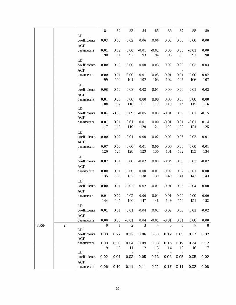
65
81 82 83 84 85 86 87 88 89
LD coefficients -0.03 0.02 -0.02 0.06 -0.06 0.02 0.00 0.00 0.00
ACF parameters 0.01 0.02 0.00 -0.01 -0.02 0.00 0.00 -0.01 0.00
90 91 92 93 94 95 96 97 98
LD coefficients 0.00 0.00 0.00 0.00 -0.03 0.02
-0.06 0.03 -0.03
ACF parameters 0.00 0.01 0.00 -0.01 0.03 -0.01
-0.01 0.00 0.02
99 100 101 102 103 104 105 106 107
LD coefficients 0.06 -0.10 0.08 -0.03 0.01 0.00 0.00 0.01 -0.02
ACF parameters 0.01 0.07 0.00 0.00 0.00 0.00 0.00 0.00 0.00
108 109 110 111 112 113 114 115 116
LD coefficients 0.04 -0.06 0.09 -0.05 0.03 -0.01 0.00 0.02 -0.15
ACF parameters 0.01 0.01 0.01 0.01 0.00 -0.01
-0.01 -0.01 0.14
117 118 119 120 121 122 123 124 125
LD coefficients 0.00 0.02 -0.01 0.00 0.02 -0.02 0.03 -0.02 0.01
ACF parameters 0.07 0.00 0.00 -0.01 0.00 0.00 0.00 0.00 -0.01
126 127 128 129 130 131 132 133 134
LD coefficients 0.02 0.01 0.00 -0.02 0.03 -0.04 0.08 0.03 -0.02
ACF parameters 0.00 0.01 0.00 0.00 -0.01 -0.02
-0.02 -0.01 0.00
135 136 137 138 139 140 141 142 143
LD coefficients 0.00 0.01 -0.02 0.02 -0.01 -0.01 0.03 -0.04 0.00
ACF parameters -0.01 -0.02 -0.02 0.00 0.01 0.01 0.00 0.00 0.00
144 145 146 147 148 149 150 151 152
LD coefficients -0.01 0.01 0.01 -0.04 0.02 -0.03 0.00 0.01 -0.02
ACF parameters 0.00 0.00 -0.01 0.04 -0.01 -0.01 0.01 0.00 0.00
FSSF 2 0 1 2 3 4 5 6 7 8
LD coefficients 1.00
-0.27 0.12
-0.06 0.03
-0.12
-0.05
-0.17 0.02
ACF parameters 1.00 0.30 0.04 0.09 0.08 0.16 0.19 0.24 0.12
9 10 11 12 13 14 15 16 17
LD coefficients 0.02 0.01
-0.03 0.05
-0.13
-0.03
-0.05 0.05 0.02
ACF parameters 0.06 0.10 0.11 0.11 0.22 0.17 0.11 0.02 0.08
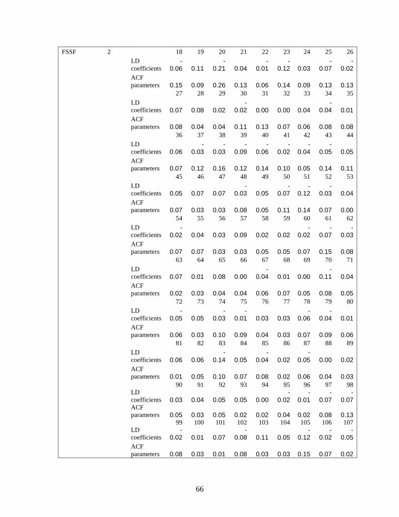
66
FSSF 2 18 19 20 21 22 23 24 25 26
LD coefficients
-0.06 0.11
-0.21 0.04
-0.01
-0.12 0.03
-0.07
-0.02
ACF parameters 0.15 0.09 0.26 0.13 0.06 0.14 0.09 0.13 0.13
27 28 29 30 31 32 33 34 35
LD coefficients 0.07 0.08 0.02
-0.02 0.00 0.00 0.04
-0.04 0.01
ACF parameters 0.08 0.04 0.04 0.11 0.13 0.07 0.06 0.08 0.08
36 37 38 39 40 41 42 43 44
LD coefficients 0.06
-0.03
-0.03
-0.09
-0.06
-0.02
-0.04
-0.05 0.05
ACF parameters 0.07 0.12 0.16 0.12 0.14 0.10 0.05 0.14 0.11
45 46 47 48 49 50 51 52 53
LD coefficients 0.05 0.07 0.07
-0.03 0.05
-0.07
-0.12
-0.03 0.04
ACF parameters 0.07 0.03 0.03 0.08 0.05 0.11 0.14 0.07 0.00
54 55 56 57 58 59 60 61 62
LD coefficients
-0.02 0.04 0.03 0.09 0.02 0.02
-0.02
-0.07
-0.03
ACF parameters 0.07 0.07 0.03 0.03 0.05 0.05 0.07 0.15 0.08
63 64 65 66 67 68 69 70 71
LD coefficients 0.07 0.01 0.08 0.00
-0.04 0.01 0.00
-0.11 0.04
ACF parameters 0.02 0.03 0.04 0.04 0.06 0.07 0.05 0.08 0.05
72 73 74 75 76 77 78 79 80
LD coefficients
-0.05 0.05
-0.03
-0.01 0.03 0.03
-0.06
-0.04 0.01
ACF parameters 0.06 0.03 0.10 0.09 0.04 0.03 0.07 0.09 0.06
81 82 83 84 85 86 87 88 89
LD coefficients 0.06 0.06
-0.14 0.05
-0.04 0.02
-0.05 0.00 0.02
ACF parameters 0.01 0.05 0.10 0.07 0.08 0.02 0.06 0.04 0.03
90 91 92 93 94 95 96 97 98
LD coefficients 0.03 0.04 0.05 0.05 0.00
-0.02
-0.01
-0.07
-0.07
ACF parameters 0.05 0.03 0.05 0.02 0.02 0.04 0.02 0.08 0.13
99 100 101 102 103 104 105 106 107
LD coefficients
-0.02 0.01 0.07
-0.08 0.11 0.05
-0.12
-0.02
-0.05
ACF parameters 0.08 0.03 0.01 0.08 0.03 0.03 0.15 0.07 0.02
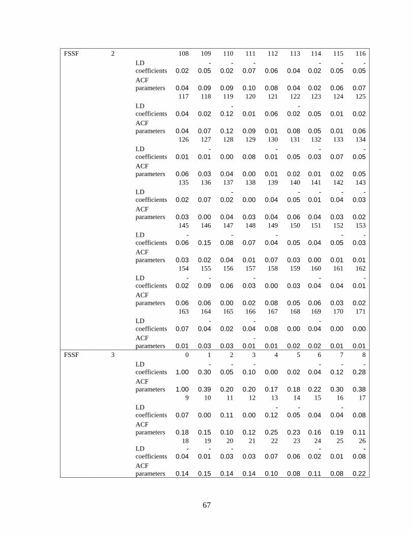
67
FSSF 2 108 109 110 111 112 113 114 115 116
LD coefficients 0.02
-0.05
-0.02
-0.07 0.06 0.04
-0.02
-0.05
-0.05
ACF parameters 0.04 0.09 0.09 0.10 0.08 0.04 0.02 0.06 0.07
117 118 119 120 121 122 123 124 125
LD coefficients 0.04 0.02
-0.12 0.01 0.06
-0.02 0.05 0.01 0.02
ACF parameters 0.04 0.07 0.12 0.09 0.01 0.08 0.05 0.01 0.06
126 127 128 129 130 131 132 133 134
LD coefficients 0.01
-0.01 0.00 0.08
-0.01 0.05
-0.03 0.07
-0.05
ACF parameters 0.06 0.03 0.04 0.00 0.01 0.02 0.01 0.02 0.05
135 136 137 138 139 140 141 142 143
LD coefficients 0.02 0.07
-0.02 0.00 0.04
-0.05
-0.01
-0.04
-0.03
ACF parameters 0.03 0.00 0.04 0.03 0.04 0.06 0.04 0.03 0.02
145 146 147 148 149 150 151 152 153
LD coefficients
-0.06 0.15
-0.08 0.07
-0.04 0.05 0.04
-0.05
-0.03
ACF parameters 0.03 0.02 0.04 0.01 0.07 0.03 0.00 0.01 0.01
154 155 156 157 158 159 160 161 162
LD coefficients
-0.02
-0.09 0.06
-0.03 0.00 0.03
-0.04 0.04
-0.01
ACF parameters 0.06 0.06 0.00 0.02 0.08 0.05 0.06 0.03 0.02
163 164 165 166 167 168 169 170 171
LD coefficients 0.07
-0.04 0.02
-0.04 0.08 0.00
-0.04 0.00 0.00
ACF parameters 0.01 0.03 0.03
-0.01 0.01 0.02 0.02 0.01 0.01
FSSF 3 0 1 2 3 4 5 6 7 8
LD coefficients 1.00
-0.30
-0.05
-0.10 0.00 0.02
-0.04
-0.12
-0.28
ACF parameters 1.00 0.39 0.20 0.20 0.17 0.18 0.22 0.30 0.38
9 10 11 12 13 14 15 16 17
LD coefficients 0.07 0.00 0.11 0.00
-0.12
-0.05 0.04
-0.04 0.08
ACF parameters 0.18 0.15 0.10 0.12 0.25 0.23 0.16 0.19 0.11
18 19 20 21 22 23 24 25 26
LD coefficients
-0.04
-0.01
-0.03 0.03 0.07 0.06
-0.02 0.01
-0.08
ACF parameters 0.14 0.15 0.14 0.14 0.10 0.08 0.11 0.08 0.22
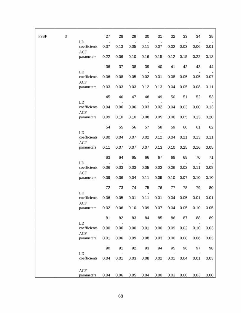
68
FSSF 3 27 28 29 30 31 32 33 34 35
LD coefficients
-0.07 0.13
-0.05
-0.11
-0.07 0.02
-0.03
-0.06
-0.01
ACF parameters 0.22 0.06 0.10 0.16 0.15 0.12 0.15 0.22 0.13
36 37 38 39 40 41 42 43 44
LD coefficients 0.06 0.08 0.05
-0.02 0.01 0.08 0.05
-0.05
-0.07
ACF parameters 0.03 0.03 0.03 0.12 0.13 0.04 0.05 0.08 0.11
45 46 47 48 49 50 51 52 53
LD coefficients 0.04
-0.06 0.06
-0.03
-0.02 0.04 0.03 0.00
-0.13
ACF parameters 0.09 0.10 0.10 0.08 0.05 0.06 0.05 0.13 0.20
54 55 56 57 58 59 60 61 62
LD coefficients 0.00
-0.04 0.07 0.02
-0.12 0.04
-0.21 0.13 0.11
ACF parameters 0.11 0.07 0.07 0.07 0.13 0.10 0.25 0.16 0.05
63 64 65 66 67 68 69 70 71
LD coefficients
-0.06
-0.03 0.03 0.05 0.03 0.06
-0.02
-0.11
-0.08
ACF parameters 0.09 0.06 0.04 0.11 0.09 0.10 0.07 0.10 0.10
72 73 74 75 76 77 78 79 80
LD coefficients 0.06 0.05 0.01
-0.11 0.01 0.04 0.05 0.01 0.01
ACF parameters 0.02 0.06 0.10 0.09 0.07 0.04 0.05 0.10 0.05
81 82 83 84 85 86 87 88 89
LD coefficients 0.00
-0.06 0.00 0.01 0.00 0.09 0.02
-0.10 0.03
ACF parameters 0.01 0.06 0.09 0.08 0.03 0.00 0.08 0.06 0.03
90 91 92 93 94 95 96 97 98
LD coefficients 0.04
-0.01 0.03
-0.08 0.02
-0.01 0.04
-0.01 0.03
ACF parameters 0.04 0.06 0.05 0.04 0.00 0.03 0.00 0.03 0.00
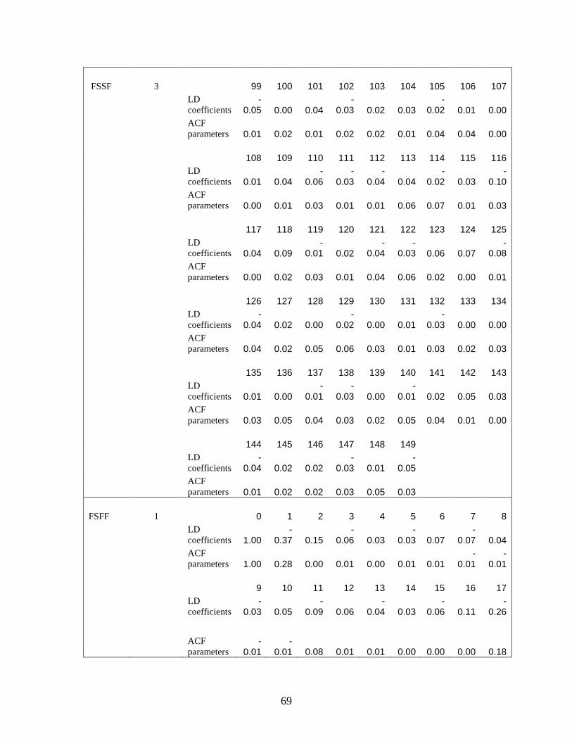
69
FSSF 3 99 100 101 102 103 104 105 106 107
LD coefficients
-0.05 0.00 0.04
-0.03 0.02 0.03
-0.02 0.01 0.00
ACF parameters 0.01 0.02 0.01 0.02 0.02 0.01 0.04 0.04 0.00
108 109 110 111 112 113 114 115 116
LD coefficients 0.01 0.04
-0.06
-0.03
-0.04 0.04
-0.02 0.03
-0.10
ACF parameters 0.00 0.01 0.03 0.01 0.01 0.06 0.07 0.01 0.03
117 118 119 120 121 122 123 124 125
LD coefficients 0.04 0.09
-0.01 0.02
-0.04
-0.03 0.06 0.07
-0.08
ACF parameters 0.00 0.02 0.03 0.01 0.04 0.06 0.02 0.00 0.01
126 127 128 129 130 131 132 133 134
LD coefficients
-0.04 0.02 0.00
-0.02 0.00 0.01
-0.03 0.00 0.00
ACF parameters 0.04 0.02 0.05 0.06 0.03 0.01 0.03 0.02 0.03
135 136 137 138 139 140 141 142 143
LD coefficients 0.01 0.00
-0.01
-0.03 0.00
-0.01 0.02 0.05 0.03
ACF parameters 0.03 0.05 0.04 0.03 0.02 0.05 0.04 0.01 0.00
144 145 146 147 148 149
LD coefficients
-0.04 0.02 0.02
-0.03 0.01
-0.05
ACF parameters 0.01 0.02 0.02 0.03 0.05 0.03
FSFF 1 0 1 2 3 4 5 6 7 8
LD coefficients 1.00
-0.37 0.15
-0.06 0.03
-0.03 0.07
-0.07 0.04
ACF parameters 1.00 0.28 0.00 0.01 0.00 0.01 0.01
-0.01
-0.01
9 10 11 12 13 14 15 16 17
LD coefficients
-0.03 0.05
-0.09 0.06
-0.04 0.03
-0.06 0.11
-0.26
ACF parameters
-0.01
-0.01 0.08 0.01 0.01 0.00 0.00 0.00 0.18
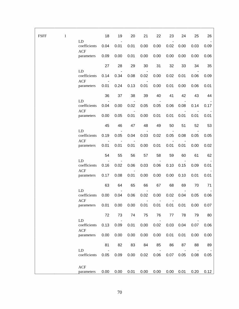
70
FSFF 1 18 19 20 21 22 23 24 25 26
LD coefficients 0.04
-0.01 0.01 0.00 0.00
-0.02 0.00 0.03
-0.09
ACF parameters 0.09 0.00 0.01 0.00 0.00 0.00 0.00 0.00 0.06
27 28 29 30 31 32 33 34 35
LD coefficients 0.14
-0.34 0.08
-0.02 0.00 0.02 0.01
-0.06 0.09
ACF parameters
-0.01 0.24 0.13
-0.01 0.00 0.01 0.00 0.06 0.01
36 37 38 39 40 41 42 43 44
LD coefficients
-0.04 0.00
-0.02 0.05
-0.05 0.06
-0.08 0.14
-0.17
ACF parameters 0.00 0.05
-0.01 0.00 0.01 0.01
-0.01
-0.01
-0.01
45 46 47 48 49 50 51 52 53
LD coefficients 0.19
-0.05 0.04
-0.03 0.02
-0.05 0.08
-0.05 0.05
ACF parameters
-0.01
-0.01
-0.01 0.00 0.01
-0.01
-0.01 0.00 0.02
54 55 56 57 58 59 60 61 62
LD coefficients
-0.16
-0.02 0.06 0.03
-0.06 0.10
-0.15 0.09
-0.01
ACF parameters 0.17 0.08
-0.01 0.00 0.00 0.00 0.10 0.01
-0.01
63 64 65 66 67 68 69 70 71
LD coefficients 0.00
-0.04 0.06
-0.02 0.00 0.02
-0.04 0.05
-0.06
ACF parameters 0.01 0.00 0.00
-0.01
-0.01
-0.01 0.01 0.00 0.07
72 73 74 75 76 77 78 79 80
LD coefficients 0.13
-0.09 0.01 0.00
-0.02 0.03 0.04
-0.07 0.06
ACF parameters 0.00 0.00 0.00 0.00 0.00 0.01 0.01 0.00 0.00
81 82 83 84 85 86 87 88 89
LD coefficients
-0.05 0.09 0.00 0.02
-0.06 0.07
-0.05
-0.08
-0.05
ACF parameters 0.00 0.00 0.01 0.00 0.00 0.00 0.01 0.20 0.12
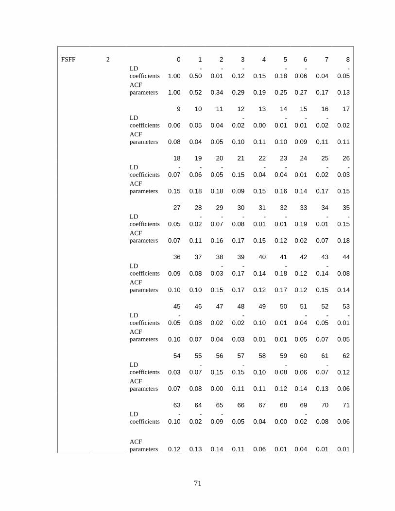
71
FSFF 2 0 1 2 3 4 5 6 7 8
LD coefficients 1.00
-0.50
-0.01
-0.12 0.15
-0.18
-0.06 0.04
-0.05
ACF parameters 1.00 0.52 0.34 0.29 0.19 0.25 0.27 0.17 0.13
9 10 11 12 13 14 15 16 17
LD coefficients 0.06 0.05 0.04
-0.02 0.00
-0.01
-0.01
-0.02 0.02
ACF parameters 0.08 0.04 0.05 0.10 0.11 0.10 0.09 0.11 0.11
18 19 20 21 22 23 24 25 26
LD coefficients
-0.07
-0.06
-0.05 0.15
-0.04
-0.04 0.01
-0.02
-0.03
ACF parameters 0.15 0.18 0.18 0.09 0.15 0.16 0.14 0.17 0.15
27 28 29 30 31 32 33 34 35
LD coefficients 0.05
-0.02
-0.07
-0.08
-0.01
-0.01 0.19
-0.01
-0.15
ACF parameters 0.07 0.11 0.16 0.17 0.15 0.12 0.02 0.07 0.18
36 37 38 39 40 41 42 43 44
LD coefficients 0.09 0.08
-0.03
-0.17 0.14
-0.18 0.12
-0.14 0.08
ACF parameters 0.10 0.10 0.15 0.17 0.12 0.17 0.12 0.15 0.14
45 46 47 48 49 50 51 52 53
LD coefficients
-0.05 0.08 0.02
-0.02 0.10 0.01
-0.04
-0.05
-0.01
ACF parameters 0.10 0.07 0.04 0.03 0.01 0.01 0.05 0.07 0.05
54 55 56 57 58 59 60 61 62
LD coefficients 0.03
-0.07 0.15
-0.15 0.10
-0.08 0.06
-0.07 0.12
ACF parameters 0.07 0.08 0.00 0.11 0.11 0.12 0.14 0.13 0.06
63 64 65 66 67 68 69 70 71
LD coefficients
-0.10
-0.02
-0.09 0.05 0.04 0.00
-0.02 0.08 0.06
ACF parameters 0.12 0.13 0.14 0.11 0.06 0.01 0.04 0.01 0.01
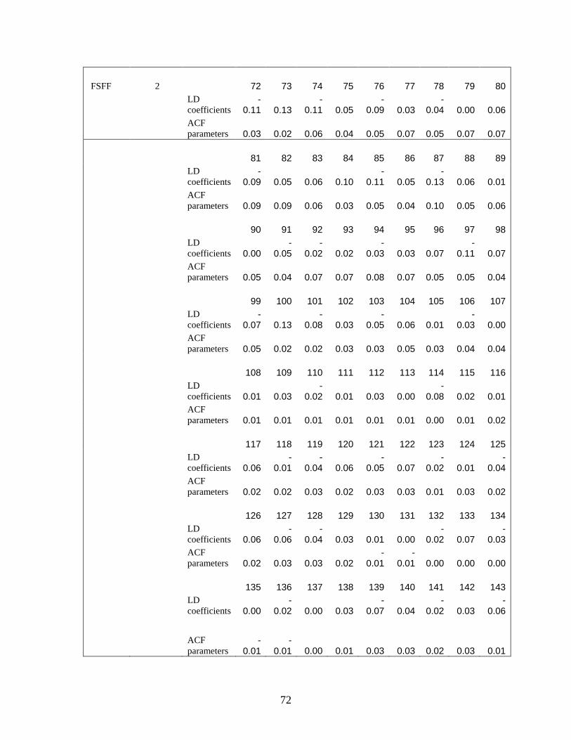
72
FSFF 2 72 73 74 75 76 77 78 79 80
LD coefficients
-0.11 0.13
-0.11 0.05
-0.09 0.03
-0.04 0.00 0.06
ACF parameters 0.03 0.02 0.06 0.04 0.05 0.07 0.05 0.07 0.07
81 82 83 84 85 86 87 88 89
LD coefficients
-0.09 0.05 0.06 0.10
-0.11 0.05
-0.13 0.06 0.01
ACF parameters 0.09 0.09 0.06 0.03 0.05 0.04 0.10 0.05 0.06
90 91 92 93 94 95 96 97 98
LD coefficients 0.00
-0.05
-0.02 0.02
-0.03 0.03 0.07
-0.11 0.07
ACF parameters 0.05 0.04 0.07 0.07 0.08 0.07 0.05 0.05 0.04
99 100 101 102 103 104 105 106 107
LD coefficients
-0.07 0.13
-0.08 0.03
-0.05 0.06 0.01
-0.03 0.00
ACF parameters 0.05 0.02 0.02 0.03 0.03 0.05 0.03 0.04 0.04
108 109 110 111 112 113 114 115 116
LD coefficients 0.01 0.03
-0.02 0.01 0.03 0.00
-0.08 0.02 0.01
ACF parameters 0.01 0.01 0.01 0.01 0.01 0.01 0.00 0.01 0.02
117 118 119 120 121 122 123 124 125
LD coefficients 0.06
-0.01
-0.04 0.06
-0.05 0.07
-0.02 0.01
-0.04
ACF parameters 0.02 0.02 0.03 0.02 0.03 0.03 0.01 0.03 0.02
126 127 128 129 130 131 132 133 134
LD coefficients 0.06
-0.06
-0.04 0.03 0.01 0.00
-0.02 0.07
-0.03
ACF parameters 0.02 0.03 0.03 0.02
-0.01
-0.01 0.00 0.00 0.00
135 136 137 138 139 140 141 142 143
LD coefficients 0.00
-0.02 0.00 0.03
-0.07 0.04
-0.02 0.03
-0.06
ACF parameters
-0.01
-0.01 0.00 0.01 0.03 0.03 0.02 0.03 0.01
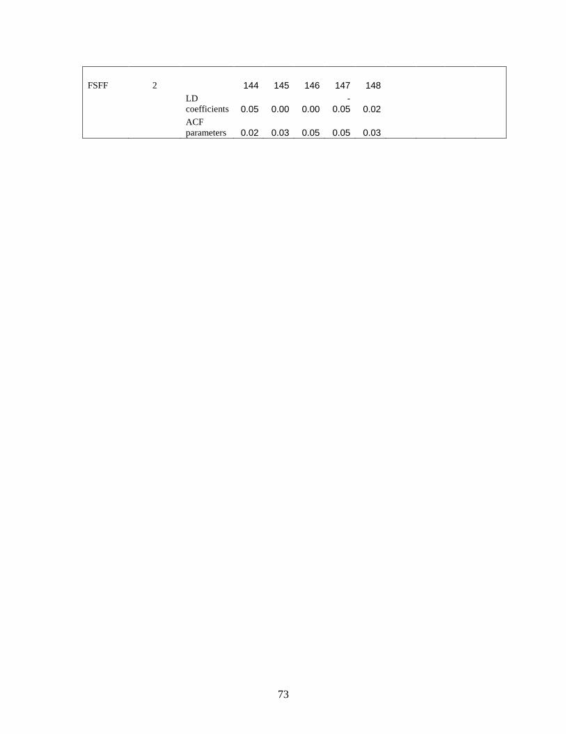
73
FSFF 2 144 145 146 147 148
LD coefficients 0.05 0.00 0.00
-0.05 0.02
ACF parameters 0.02 0.03 0.05 0.05 0.03
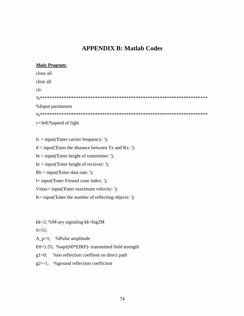
74
APPENDIX B: Matlab Codes
Main Program:
close all
clear all
clc
%************************************************** ********************
%Input parameters
%************************************************** ********************
c=3e8;%speed of light
fc = input('Enter carrier frequency: ');
d = input('Enter the distance between Tx and Rx: ');
ht = input('Enter height of transmitter: ');
hr = input('Enter height of receiver: ');
Rb = input('Enter data rate: ');
l= input('Enter Fresnel zone index: ');
Vmax= input('Enter maximum velocity: ');
K= input('Enter the number of reflecting objects: ');
kk=2; %M-ary signaling kk=log2M
S=51;
A_p=1; %Pulse amplitude
E0=1.55; %sqrt(60*EIRP)- transmitted field strength
g1=0; %no reflection coeffient on direct path
g2=-1; %ground reflection coefficient
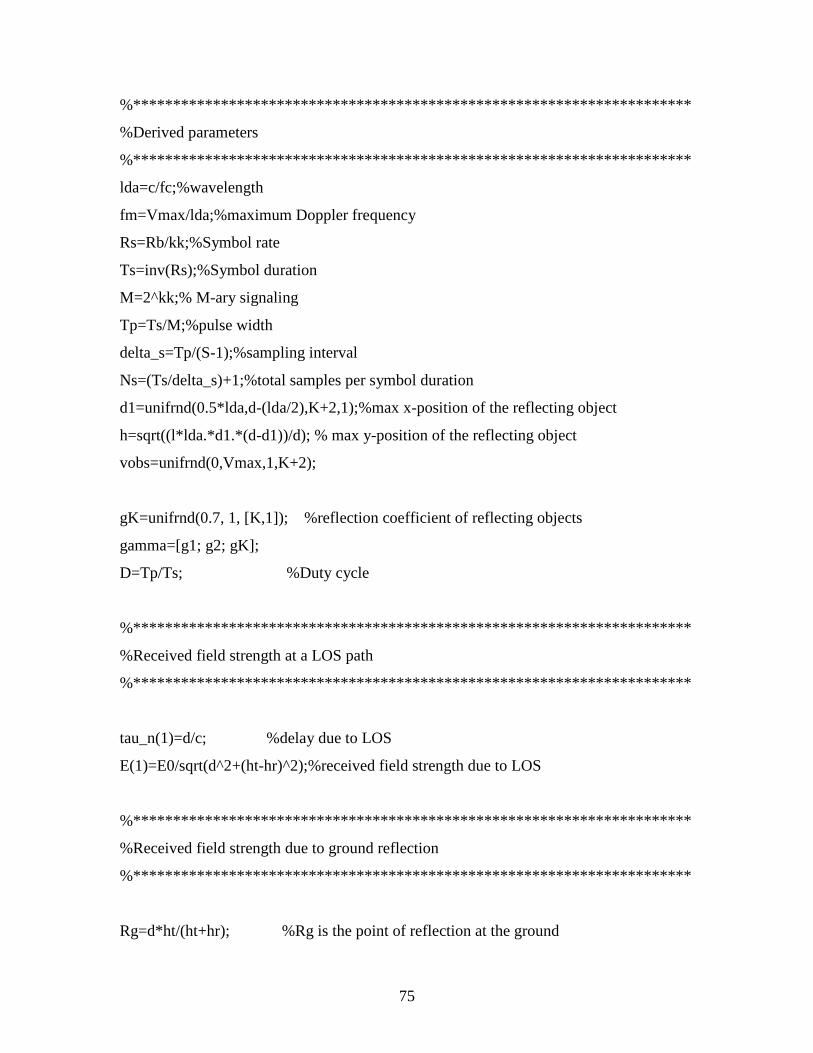
75
%************************************************** ********************
%Derived parameters
%************************************************** ********************
lda=c/fc;%wavelength
fm=Vmax/lda;%maximum Doppler frequency
Rs=Rb/kk;%Symbol rate
Ts=inv(Rs);%Symbol duration
M=2^kk;% M-ary signaling
Tp=Ts/M;%pulse width
delta_s=Tp/(S-1);%sampling interval
Ns=(Ts/delta_s)+1;%total samples per symbol duration
d1=unifrnd(0.5*lda,d-(lda/2),K+2,1);%max x-position of the reflecting object
h=sqrt((l*lda.*d1.*(d-d1))/d); % max y-position of the reflecting object
vobs=unifrnd(0,Vmax,1,K+2);
gK=unifrnd(0.7, 1, [K,1]); %reflection coefficient of reflecting objects
gamma=[g1; g2; gK];
D=Tp/Ts; %Duty cycle
%************************************************** ********************
%Received field strength at a LOS path
%************************************************** ********************
tau_n(1)=d/c; %delay due to LOS
E(1)=E0/sqrt(d^2+(ht-hr)^2);%received field strength due to LOS
%************************************************** ********************
%Received field strength due to ground reflection
%************************************************** ********************
Rg=d*ht/(ht+hr); %Rg is the point of reflection at the ground
76
dd1(2)=sqrt(ht^2+Rg^2); %distance travelled by incident signal
dd2(2)=sqrt(hr^2+(d-Rg)^2); %distance travelled by reflected signal
tau_n(2)=(dd1(2)+dd2(2))/c; %delay due to ground reflection
E(2)=gamma(2)*E0/(dd1(2)+dd2(2));%received field strength due to ground
%reflection
% ************************************************* ********************
%Received field strength due to reflecting objects in the space
% ************************************************* ********************
for n=3:K+2
hobs(n) = unifrnd(0,h(n),1,1);
dd1(n)=sqrt((d1(n))^2+(hobs(n)-ht)^2); %transmitter-obstacle distance
dd2(n)=sqrt((d-d1(n))^2+(hobs(n)-hr)^2); %obstacle - receiver distance
E(n)=E0*gamma(n)/(dd1(n)+dd2(n)); %field strength amplitude
tau_n(n)=(dd1(n)+dd2(n))/c; %delay due to reflectin objects
end
tau=tau_n; %delay vector
EdB=10*log10(E); % field strength amplitude in dB
% ************************************************* ********************
% Received pulses at each multipath delay
% ************************************************* ********************
for j=1:20
Tdist=[d dd2(2:end)]; %array of distance after reflection
v=[Vmax vobs(2:end)];
theta=rand(1,K+2)*2*pi-pi; %angle of arrival at the terminal
alpha=E; %each path field strength amplitude
77
delay=2*pi*fc*tau; %delay of each multipath
doppler=(2*pi*(v.*cos(theta)*fc)/c).*Tdist;
tm=1:Ns*40;
for k=1:K+2
for m=1:Ns*40
tlower(k)=tau(k); %lower bound of time scale after delay
t(k,m)=tlower(k)+(m-1)*Ts/(Ns-1); %time steps associated with each delay
if m < round(tlower(k)/delta_s)
rt_in(k,m)=0;
rt_q(k,m)=0;
rt_env(k,m)=0;
elseif m==round(tlower(k)/delta_s)% & m<=round(D*Ns)
rt_in(k,m)=alpha(k)*cos(delay(k)+doppler(k));
rt_q(k,m)=alpha(k)*sin(delay(k)+doppler(k));
rt_env(k,m)=sqrt(rt_in(k,m)^2+rt_q(k,m)^2);
p(k,m)=A_p; %first part of input pulse
else
rt_in(k,m)=0;
rt_q(k,m)=0;
rt_env(k,m)=0;
p(k,m)=0*A_p; %second part of input pulse
end
end
end
rt_sum=sum(rt_env);
RP(j,:)=rt_sum;
end
t_scale=round(tlower/delta_s);
RP_mean=mean(RP);
78
ReceivedPulse=RP_mean((min(t_scale)):(max(t_scale)));
time=tm(min(t_scale):max(t_scale));
RPpwr=ReceivedPulse.^2;
%************************************************** ********************
%Autocorrelation of the generic data
%************************************************** ********************
[nom_A_C,lags]=xcorr(ReceivedPulse,'coeff'); %normalized ACF of the received
signal
%************************************************** ********************
%Building an autoregressive model
%************************************************** ********************
length=size(lags);
mid_pt=round(length(2)/2);
for i=1:20
AC_GENERIC=nom_A_C(mid_pt:end); %Half side of the ACF from generic
model
[AR_Coeff, var]=rtoa(AC_GENERIC); %AR coefficients from the ACF_gen +
variance
noise=sqrt(var)*randn(1000,1); %noise as input to AR model
wgnfil=filter(1,AR_Coeff,noise); %AR model driven by noise with variance, var
[filcoeff,error_LD]=acm(wgnfil,mid_pt-1); %filter coefficient of signal reproduced
by AR model
AC_AR=ator(filcoeff); %Half side of the ACF of AR reproduced signal
flip_AC_AR=fliplr(AC_AR);
AC_AR_fct_Full_length=[flip_AC_AR AC_AR(2:end)];
AC_AR_fct_matrix(i,:)=AC_AR_fct_Full_length;
end
AC_AR_fct=sum(AC_AR_fct_matrix)/i; %ACF of AR reproduced signal
79
t_lag=sort(tau/delta_s);
%************************************************** ********************
%Mean Square Error Calculations
%************************************************** ********************
vect_error=(nom_A_C-AC_AR_fct).^2; %square error of the two ACFs
mse=mean(vect_error) %Mean square error
%************************************************** ********************
% RMS delay spread and coherence time
%************************************************** ********************
mean_excessdelay=sum(RPpwr.*time*delta_s)/sum(RPpwr); %mean excess delay
MEDsquare=sum((delta_s*time).^2.*RPpwr)/sum(RPpwr); %mean square excess
delay
rms_delay_spread=sqrt(MEDsquare-mean_excessdelay^2) %rms delay spread
T_c=0.423/fm %channel's coherence time
Ts %symbol duration
delta_tau=delta_s*1e9
AR_Coeff
ACF=AC_AR_fct'
%************************************************** ********************
%Different Plots
%************************************************** ********************
figure(1);
stem(time,ReceivedPulse*1e3)
xlabel('Time in units of \Delta\it\tau')
80
ylabel('Received signal amplitude (mV)')
figure(2);
stem(time,10*log10(RPpwr))
xlabel('Time in units of \Delta\it\tau')
ylabel('Received signal power (dB)')
figure(3);
stem(lags,nom_A_C,'b*')
hold on
stem(lags,AC_AR_fct,'ro')
xlabel('Time lag in units of \rm\Delta\it\tau ')
ylabel('Autocorrelation function')
legend('Channel Model','AR Model')
figure(4);
stem(wgnfil(950:end))
xlabel('Sample time in units of \rm\Delta\it\tau ')
ylabel('Received signal(mV)')
Levinson-Durbin recursion: From autocorrelation function to AR coefficients [Hay96]
function [a,epsilon]=rtoa(r)
%RTOA Levinson-Durbin recursion.
%----
%USAGE: [a,epsilon]=rtoa(r)
%
% Solves the Toeplitz normal equations
% R a = epsilon [1 0 ... 0]'
% where R=toeplitz(r) is a Toeplitz matrix that contains
81
% the autocorrelation sequence r(k). The ouputs are the
% coefficients of the all-pole model a(k) and the constant
% epsilon.
%---------------------------------------------------------------
r=r(:);
p=length(r)-1;
a=1;
epsilon=r(1);
for j=2:p+1;
gamma=-r(2:j)'*flipud(a)/epsilon;
a=[a;0] + gamma*[0;conj(flipud(a))];
epsilon=epsilon*(1 - abs(gamma)^2);
end
Inverse Levinson-Durbin recursion: From AR coefficients to autocorrelation function
[Hay96]
function r=ator(a,b)
%ATOR Inverse Levinson-Durbin recursion.
%----
%USAGE: r=ator(a,b)
% Finds the autocorrelation sequence r(k) of an
% autoregressive process that is generated by
% filtering unit variance white noise with the filter
% H(z)=b(0)/A(z)
% With r = ator(a) the autocorrelation sequence is
% normalized so that r(0)=1.
%
% see also ATOG, GTOA, GTOR, RTOA, RTOG
82
%---------------------------------------------------------------
% copyright 1996, by M.H. Hayes. For use with the book
% "Statistical Digital Signal Processing and Modeling"
% (John Wiley & Sons, 1996).
%---------------------------------------------------------------
p=length(a)-1;
gamma=atog(a);
r=gtor(gamma);
if nargin == 2,
r = r*b^2/prod(1-abs(gamma).^2);
end;
83
BIBLIOGRAPHY
[You00] David J. Young, ‘The Generation of Correlated Rayleigh Random Varietes by Inverse Discrete Fourier Transform’, IEEE Transactions on Communications, Vol 48, no. 7, July 2000
[Bad05] Kareem E. Baddour, Norman C. Beaulieu, ‘Autoregressive Modeling for
Fading Channel Simulations’, IEEE Trans on Wireless Communications, Vol. 4, no. 4, July 2005
[Mat05] Suhas Mathur, ‘Small Scale Fading’, Rutgar University, 2005 [Hay96] Monson H, Hayes, Statistical Digital Signal Processing and Modeling,
John wiley & Sons, Inc., New Jersey, 1996 [Pap91] A. Papoulis, Probability, Random Variables and Stochastic Processes, 3rd
Edition, McGraw Hill New York, 1991 [Vau03] Vaughan, Rodney and Anderson, Jørgen Bach, Channels, Propagation
and Antennas for Mobile Communications, Institute of Electical Engineers, 2003
[Gol05] Andrea Goldsmith, Wireless Communications. Cambridge University
Press, 2005 [Rap02] T. S. Rappaport, Wireless Communications, Principles and Practice,
Prentice Hall, New Jersey, 1996 [Ath 00] G. E. Athanasiadou, A. R. Nix, and J. P. McGreehan, “A microcellular
ray- tracing propagation model and evaluation of its narrowband and wideband predictions,” IEEE Journal on Selected Areas in Communications, Wireless Communications series, vol. 18, pp. 322-335, March 2000
[Cou01] Leon W. Couch, II, Digital and Analog Communication systems, Prentice
Hall, New Jersey, 2001 [Bla07] Nathan Blaunstein, Christos G. Christodoulou, Radio Propagation and
Adaptive Antennas for Wireless Communications Links, John Wiley & Sons, Inc., New Jersey, 2007
84
BIOGRAPHICAL SKETCH
Mahinga Hekeno was born and raised in Dar-es-Salaam, Tanzania. She is currently a
Master’s student of Electrical and Computer Engineering at Florida State University. Her
Master’s thesis research is on statistical modeling of small-scale fading channels, and is
under the direction of Professor Bing W. Kwan.
She has been a master’s student in Electrical and Computer Engineering at Florida State
University since January 2006. She has also held a Bachelors of Science degree in
Electrical and Electronic Engineering from Department of Electrical and Computer
Engineering of California State University, Sacramento.