Provide feedback about this page Fading Channelsmdoniak/CDI_20705/Fading%20... · Fading Channels :: Channels (Communications Toolbox™) jar: ... In the example below, entering c1

Fading Channels :: Channels (Communications Toolbox™) jar:file:///C:/Arquivos%20de%20programas/MATLAB/R2008a/help/too...

1 of 23 3/10/2013 08:43

Communications Toolbox™ Provide feedback about this page

Fading Channels

On this page…

Section OverviewOverview of Fading ChannelsSimulation of Multipath Fading Channels: MethodologySpecifying Fading ChannelsSpecifying the Doppler Spectrum of a Fading ChannelConfiguring Channel ObjectsUsing Fading ChannelsExamples Using Fading ChannelsUsing the Channel Visualization Tool

Section OverviewRayleigh and Rician fading channels are useful models of real-world phenomena in wireless communications. Thesephenomena include multipath scattering effects, time dispersion, and Doppler shifts that arise from relative motionbetween the transmitter and receiver. This section gives a brief overview of fading channels and describes how toimplement them using the toolbox.

Back to Top

Overview of Fading ChannelsThe figure below depicts direct and major reflected paths between a stationary radio transmitter and a moving receiver.The shaded shapes represent reflectors such as buildings.

The major paths result in the arrival of delayed versions of the signal at the receiver. In addition, the radio signalundergoes scattering on a local scale for each major path. Such local scattering is typically characterized by a largenumber of reflections by objects near the mobile. These irresolvable components combine at the receiver and give rise tothe phenomenon known as multipath fading. Due to this phenomenon, each major path behaves as a discrete fadingpath. Typically, the fading process is characterized by a Rayleigh distribution for a nonline-of-sight path and a Riciandistribution for a line-of-sight path.

The relative motion between the transmitter and receiver causes Doppler shifts. Local scattering typically comes frommany angles around the mobile. This scenario causes a range of Doppler shifts, known as the Doppler spectrum. The maximum Doppler shift corresponds to the local scattering components whose direction exactly opposes the mobile'strajectory.

Fading Channel Features of the ToolboxThe toolbox implements a baseband channel model for multipath propagation scenarios that include

N discrete fading paths, each with its own delay and average power gain. A channel for which N = 1 is called afrequency-flat fading channel. A channel for which N > 1 is experienced as a frequency-selective fading channel bya signal of sufficiently wide bandwidth.


2 of 23 3/10/2013 08:43

A Rayleigh or Rician model for each path.By default, each path of the channel is modeled with a Jakes Doppler spectrum, with a maximum Doppler shift thatcan be specified. Other types of Doppler spectra are allowed (identical or different for all paths): flat, restrictedJakes, asymmetrical Jakes, Gaussian, bi-Gaussian, and rounded.If the maximum Doppler shift is set to 0 or omitted during the construction of a channel object, then the channel ismodeled as static (i.e., the fading does not evolve with time), and the Doppler spectrum specified has no effect onthe fading process.

Some additional information about typical values for delays and gains is in Choosing Realistic Channel Property Values.

Back to Top

Simulation of Multipath Fading Channels: MethodologyThe Rayleigh and Rician multipath fading channel simulators of this toolbox use the band-limited discrete multipathchannel model of section 9.1.3.5.2 in [1]. It is assumed that the delay power profile and the Doppler spectrum of thechannel are separable [1]. The multipath fading channel is therefore modeled as a linear finite impulse-response (FIR)filter. Let denote the set of samples at the input to the channel. Then the samples at the output of the channel

are related to through:

where is the set of tap weights given by:

In the equations above:

is the input sample period to the channel.

, where , is the set of path delays. K is the total number of paths in the multipath fading channel.

, where , is the set of complex path gains of the multipath fading channel. These path gains areuncorrelated with each other.

and are chosen so that is small when n is less than or greater than .

Each path gain process is generated by the following steps:

A complex uncorrelated (white) Gaussian process with zero mean and unit variance is generated in discrete time.1.

The complex Gaussian process is filtered by a Doppler filter with frequency response , where denotes the desired Doppler power spectrum.

2.

The filtered complex Gaussian process is interpolated so that its sample period is consistent with that of the inputsignal. A combination of linear and polyphase interpolation is used.

3.

The resulting complex process is scaled to obtain the correct average path gain. In the case of a Rayleighchannel, the fading process is obtained as:

where

In the case of a Rician channel, the fading process is obtained as:

4.


3 of 23 3/10/2013 08:43

where is the Rician K-factor of the k-th path, is the Doppler shift of the line-of-sight component of the

k-th path (in Hz), and is the initial phase of the line-of-sight component of the k-th path (in rad).

At the input to the band-limited multipath channel model, the transmitted symbols must be oversampled by a factor atleast equal to the bandwidth expansion factor introduced by pulse shaping. For example, if sinc pulse shaping is used, forwhich the bandwidth of the pulse-shaped signal is equal to the symbol rate, then the bandwidth expansion factor is 1, and,in the ideal case, at least one sample-per-symbol is required at the input to the channel. If a raised cosine (RC) filter witha factor in excess of 1 is used, for which the bandwidth of the pulse-shaped signal is equal to twice the symbol rate, thenthe bandwidth expansion factor is 2, and, in the ideal case, at least two samples-per-symbol are required at the input tothe channel.

References[1] Jeruchim, M. C., Balaban, P., and Shanmugan, K. S., Simulation of Communication Systems, Second Edition, NewYork, Kluwer Academic/Plenum, 2000.

Back to Top

Specifying Fading ChannelsThis toolbox models a fading channel as a linear FIR filter. Filtering a signal using a fading channel involves these steps:

Create a channel object that describes the channel that you want to use. A channel object is a type of MATLABvariable that contains information about the channel, such as the maximum Doppler shift.

1.

Adjust properties of the channel object, if necessary, to tailor it to your needs. For example, you can change thepath delays or average path gains.

2.

Apply the channel object to your signal using the filter function.3.

This section describes how to define, inspect, and manipulate channel objects. The topics are:

Creating Channel ObjectsViewing Object PropertiesChanging Object PropertiesLinked Properties of Channel Objects

Creating Channel ObjectsThe rayleighchan and ricianchan functions create fading channel objects. The table below indicates the situationsin which each function is suitable.

Function Object Situation Modeled

rayleighchan Rayleigh fading channel object One or more major reflected paths

ricianchan Rician fading channel object One direct line-of-sight path, possibly combined with one or more majorreflected paths

For example, the command below creates a channel object representing a Rayleigh fading channel that acts on a signalsampled at 100,000 Hz. The maximum Doppler shift of the channel is 130 Hz.

c1 = rayleighchan(1/100000,130); % Rayleigh fading channel object

The object c1 is a valid input argument for the filter function. To learn how to use the filter function to filter a signal using a channel object, see Using Fading Channels.

Duplicating and Copying Objects. Another way to create an object is to duplicate an existing object and then adjustthe properties of the new object, if necessary. If you do this, it is important to use a copy command such as

c2 = copy(c1); % Copy c1 to create an independent c2.

instead of c2 = c1. The copy command creates a copy of c1 that is independent of c1. By contrast, the command c2

®


4 of 23 3/10/2013 08:43

= c1 creates c2 as merely a reference to c1, so that c1 and c2 always have indistinguishable content.

Viewing Object PropertiesA channel object has numerous properties that record information about the channel model, about the state of a channelthat has already filtered a signal, and about the channel's operation on a future signal. You can view the properties inthese ways:

To view all properties of a channel object, enter the object's name in the Command Window.To view a specific property of a channel object or to assign the property's value to a variable, enter the object'sname followed by a dot (period), followed by the name of the property.

In the example below, entering c1 causes MATLAB to display all properties of the channel object c1. Some of the properties have values from the rayleighchan command that created c1, while other properties have default values.

c1 = rayleighchan(1/100000,130); % Create object.c1 % View all properties of c1.g = c1.PathGains % Retrieve the PathGains property of c1.

The output is

c1 = ChannelType: 'Rayleigh' InputSamplePeriod: 1.0000e-005 DopplerSpectrum: [1x1 doppler.jakes] MaxDopplerShift: 130 PathDelays: 0 AvgPathGaindB: 0 NormalizePathGains: 1 StoreHistory: 0 StorePathGains: 0 PathGains: 0.2104 - 0.6197i ChannelFilterDelay: 0 ResetBeforeFiltering: 1 NumSamplesProcessed: 0

g =

0.2104 - 0.6197i

A Rician fading channel object has an additional property that does not appear above, namely, a scalar KFactorproperty.

For more information about what each channel property means, see the reference page for the rayleighchan or ricianchan function.

Changing Object PropertiesTo change the value of a writeable property of a channel object, issue an assignment statement that uses dot notation onthe channel object. More specifically, dot notation means an expression that consists of the object's name, followed by adot, followed by the name of the property.

The example below illustrates how to change the ResetBeforeFiltering property, indicating you do not want to reset the channel before each filtering operation.

c1 = rayleighchan(1/100000,130) % Create object.c1.ResetBeforeFiltering = 0 % Do not reset before filtering.

The output below displays all the properties of the channel object before and after the change in the value of theResetBeforeFiltering property. In the second listing of properties, the ResetBeforeFiltering property has the value 0.

c1 = ChannelType: 'Rayleigh' InputSamplePeriod: 1.0000e-005


5 of 23 3/10/2013 08:43

DopplerSpectrum: [1x1 doppler.jakes] MaxDopplerShift: 130 PathDelays: 0 AvgPathGaindB: 0 NormalizePathGains: 1 StoreHistory: 0 StorePathGains: 0 PathGains: 0.2104 - 0.6197i ChannelFilterDelay: 0 ResetBeforeFiltering: 1 NumSamplesProcessed: 0 c1 = ChannelType: 'Rayleigh' InputSamplePeriod: 1.0000e-005 DopplerSpectrum: [1x1 doppler.jakes] MaxDopplerShift: 130 PathDelays: 0 AvgPathGaindB: 0 NormalizePathGains: 1 StoreHistory: 0 StorePathGains: 0 PathGains: 0.2104 - 0.6197i ChannelFilterDelay: 0 ResetBeforeFiltering: 0 NumSamplesProcessed: 0

Note Some properties of a channel object are read-only. For example, you cannot assign a new value to theNumSamplesProcessed property because the channel automatically counts the number of samples it hasprocessed since the last reset.

Linked Properties of Channel ObjectsSome properties of an channel object are related to each other such that when one property's value changes, anotherproperty's value must change in some corresponding way to keep the channel object consistent. For example, if youchange the vector length of PathDelays, then the value of AvgPathGaindB must change so that its vector lengthequals that of the new value of PathDelays. This is because the length of each of the two vectors equals the number ofdiscrete paths of the channel. For details about linked properties and an example, see the reference page forrayleighchan or ricianchan.

Back to Top

Specifying the Doppler Spectrum of a Fading ChannelThe Doppler spectrum of a channel object is specified through its DopplerSpectrum property. The value of this propertymust be either:

A Doppler object. In this case, the same Doppler spectrum applies to each path of the channel object.A vector of Doppler objects of the same length as the PathDelays vector property. In this case, the Dopplerspectrum of each path is given by the corresponding Doppler object in the vector.

A Doppler object contains all the properties used to characterize the Doppler spectrum, with the exception of themaximum Doppler shift, which is a property of the channel object. This section describes how to create and manipulateDoppler objects, and how to assign them to the DopplerSpectrum property of channel objects.

Creating Doppler ObjectsThe sole purpose of Doppler objects is to specify the value of the DopplerSpectrum property of channel objects.Doppler objects can be created using one of seven functions: doppler.ajakes, doppler.bigaussian, doppler.jakes, doppler.rjakes, doppler.flat, doppler.gaussian, and doppler.rounded. For a description of each of these functions and the underlying theory, refer to their corresponding reference pages.

For example, a Gaussian spectrum with a normalized (by the maximum Doppler shift of the channel) standard deviation of0.1, can be created as:


6 of 23 3/10/2013 08:43

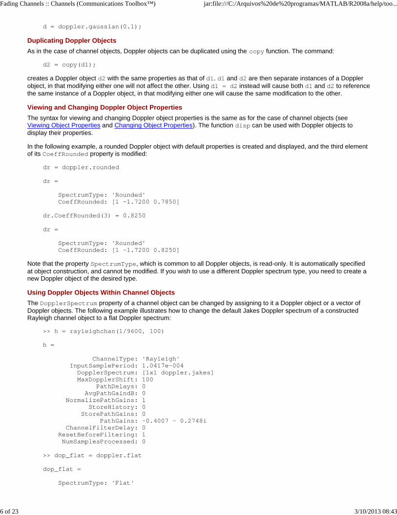
d = doppler.gaussian(0.1);

Duplicating Doppler ObjectsAs in the case of channel objects, Doppler objects can be duplicated using the copy function. The command:

d2 = copy(d1);

creates a Doppler object d2 with the same properties as that of d1. d1 and d2 are then separate instances of a Dopplerobject, in that modifying either one will not affect the other. Using d1 = d2 instead will cause both d1 and d2 to reference the same instance of a Doppler object, in that modifying either one will cause the same modification to the other.

Viewing and Changing Doppler Object PropertiesThe syntax for viewing and changing Doppler object properties is the same as for the case of channel objects (seeViewing Object Properties and Changing Object Properties). The function disp can be used with Doppler objects todisplay their properties.

In the following example, a rounded Doppler object with default properties is created and displayed, and the third elementof its CoeffRounded property is modified:

dr = doppler.rounded dr = SpectrumType: 'Rounded' CoeffRounded: [1 -1.7200 0.7850]

dr.CoeffRounded(3) = 0.8250 dr = SpectrumType: 'Rounded' CoeffRounded: [1 -1.7200 0.8250]

Note that the property SpectrumType, which is common to all Doppler objects, is read-only. It is automatically specifiedat object construction, and cannot be modified. If you wish to use a different Doppler spectrum type, you need to create anew Doppler object of the desired type.

Using Doppler Objects Within Channel ObjectsThe DopplerSpectrum property of a channel object can be changed by assigning to it a Doppler object or a vector ofDoppler objects. The following example illustrates how to change the default Jakes Doppler spectrum of a constructedRayleigh channel object to a flat Doppler spectrum:

>> h = rayleighchan(1/9600, 100) h = ChannelType: 'Rayleigh' InputSamplePeriod: 1.0417e-004 DopplerSpectrum: [1x1 doppler.jakes] MaxDopplerShift: 100 PathDelays: 0 AvgPathGaindB: 0 NormalizePathGains: 1 StoreHistory: 0 StorePathGains: 0 PathGains: -0.4007 - 0.2748i ChannelFilterDelay: 0 ResetBeforeFiltering: 1 NumSamplesProcessed: 0

>> dop_flat = doppler.flat dop_flat = SpectrumType: 'Flat'


7 of 23 3/10/2013 08:43

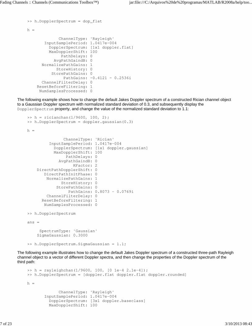
>> h.DopplerSpectrum = dop_flat h = ChannelType: 'Rayleigh' InputSamplePeriod: 1.0417e-004 DopplerSpectrum: [1x1 doppler.flat] MaxDopplerShift: 100 PathDelays: 0 AvgPathGaindB: 0 NormalizePathGains: 1 StoreHistory: 0 StorePathGains: 0 PathGains: -0.4121 - 0.2536i ChannelFilterDelay: 0 ResetBeforeFiltering: 1 NumSamplesProcessed: 0

The following example shows how to change the default Jakes Doppler spectrum of a constructed Rician channel objectto a Gaussian Doppler spectrum with normalized standard deviation of 0.3, and subsequently display theDopplerSpectrum property, and change the value of the normalized standard deviation to 1.1:

>> h = ricianchan(1/9600, 100, 2);>> h.DopplerSpectrum = doppler.gaussian(0.3) h = ChannelType: 'Rician' InputSamplePeriod: 1.0417e-004 DopplerSpectrum: [1x1 doppler.gaussian] MaxDopplerShift: 100 PathDelays: 0 AvgPathGaindB: 0 KFactor: 2 DirectPathDopplerShift: 0 DirectPathInitPhase: 0 NormalizePathGains: 1 StoreHistory: 0 StorePathGains: 0 PathGains: 0.8073 - 0.0769i ChannelFilterDelay: 0 ResetBeforeFiltering: 1 NumSamplesProcessed: 0

>> h.DopplerSpectrum ans = SpectrumType: 'Gaussian' SigmaGaussian: 0.3000

>> h.DopplerSpectrum.SigmaGaussian = 1.1;

The following example illustrates how to change the default Jakes Doppler spectrum of a constructed three-path Rayleighchannel object to a vector of different Doppler spectra, and then change the properties of the Doppler spectrum of thethird path:

>> h = rayleighchan(1/9600, 100, [0 1e-4 2.1e-4]);>> h.DopplerSpectrum = [doppler.flat doppler.flat doppler.rounded] h = ChannelType: 'Rayleigh' InputSamplePeriod: 1.0417e-004 DopplerSpectrum: [3x1 doppler.baseclass] MaxDopplerShift: 100


8 of 23 3/10/2013 08:43

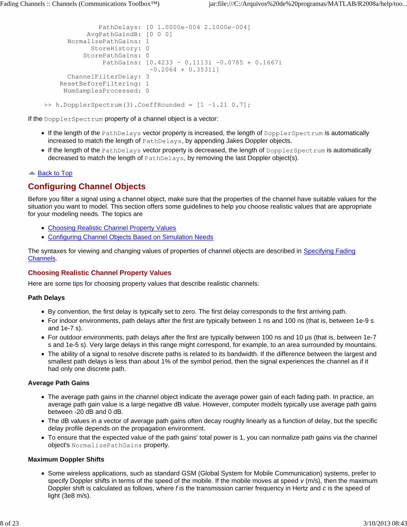
PathDelays: [0 1.0000e-004 2.1000e-004] AvgPathGaindB: [0 0 0] NormalizePathGains: 1 StoreHistory: 0 StorePathGains: 0 PathGains: [0.4233 - 0.1113i -0.0785 + 0.1667i -0.2064 + 0.3531i] ChannelFilterDelay: 3 ResetBeforeFiltering: 1 NumSamplesProcessed: 0

>> h.DopplerSpectrum(3).CoeffRounded = [1 -1.21 0.7];

If the DopplerSpectrum property of a channel object is a vector:

If the length of the PathDelays vector property is increased, the length of DopplerSpectrum is automatically increased to match the length of PathDelays, by appending Jakes Doppler objects.If the length of the PathDelays vector property is decreased, the length of DopplerSpectrum is automatically decreased to match the length of PathDelays, by removing the last Doppler object(s).

Back to Top

Configuring Channel ObjectsBefore you filter a signal using a channel object, make sure that the properties of the channel have suitable values for thesituation you want to model. This section offers some guidelines to help you choose realistic values that are appropriatefor your modeling needs. The topics are

Choosing Realistic Channel Property ValuesConfiguring Channel Objects Based on Simulation Needs

The syntaxes for viewing and changing values of properties of channel objects are described in Specifying Fading Channels.

Choosing Realistic Channel Property ValuesHere are some tips for choosing property values that describe realistic channels:

Path Delays

By convention, the first delay is typically set to zero. The first delay corresponds to the first arriving path.For indoor environments, path delays after the first are typically between 1 ns and 100 ns (that is, between 1e-9 sand 1e-7 s).For outdoor environments, path delays after the first are typically between 100 ns and 10 µs (that is, between 1e-7s and 1e-5 s). Very large delays in this range might correspond, for example, to an area surrounded by mountains.The ability of a signal to resolve discrete paths is related to its bandwidth. If the difference between the largest andsmallest path delays is less than about 1% of the symbol period, then the signal experiences the channel as if ithad only one discrete path.

Average Path Gains

The average path gains in the channel object indicate the average power gain of each fading path. In practice, anaverage path gain value is a large negative dB value. However, computer models typically use average path gainsbetween -20 dB and 0 dB. The dB values in a vector of average path gains often decay roughly linearly as a function of delay, but the specificdelay profile depends on the propagation environment.To ensure that the expected value of the path gains' total power is 1, you can normalize path gains via the channelobject's NormalizePathGains property.

Maximum Doppler Shifts

Some wireless applications, such as standard GSM (Global System for Mobile Communication) systems, prefer tospecify Doppler shifts in terms of the speed of the mobile. If the mobile moves at speed v (m/s), then the maximum Doppler shift is calculated as follows, where f is the transmission carrier frequency in Hertz and c is the speed oflight (3e8 m/s).


9 of 23 3/10/2013 08:43

Based on this formula in terms of the speed of the mobile, a signal from a moving car on a freeway mightexperience a maximum Doppler shift of about 80 Hz, while a signal from a moving pedestrian might experience amaximum Doppler shift of about 4 Hz. These figures assume a transmission carrier frequency of 900 MHz.A maximum Doppler shift of 0 corresponds to a static channel that comes from a Rayleigh or Rician distribution.

K-Factor for Rician Fading Channels

The Rician K-factor specifies the ratio of specular-to-diffuse power for a direct line-of-sight path. The ratio isexpressed linearly, not in dB.For Rician fading, the K-factor is typically between 1 and 10.A K-factor of 0 corresponds to Rayleigh fading.

Doppler Spectrum Parameters

See the reference pages for the respective Doppler objects for descriptions of the parameters and theirsignificance.

Configuring Channel Objects Based on Simulation NeedsHere are some tips for configuring a channel object to customize the filtering process:

If your data is partitioned into a series of vectors (that you process within a loop, for example), you can invoke thefilter function multiple times while automatically saving the channel's state information for use in a subsequentinvocation. The state information is visible to you in the channel object's PathGains and NumSamplesProcessed properties, but also involves properties that are internal rather than visible.

Note To maintain continuity from one invocation to the next, you must set theResetBeforeFiltering property of the channel object to 0.

If you set the ResetBeforeFiltering property of the channel object to 0 and want the randomness to berepeatable, use the reset function before filtering any signals to reset both the channel and the state of theinternal random number generator.If you want to reset the channel before a filtering operation so that it does not use any previously stored stateinformation, either use the reset function or set the ResetBeforeFiltering property of the channel object to 1. The former method resets the channel object once, while the latter method causes the filter function to resetthe channel object each time you invoke it.If you want to normalize the fading process so that the expected value of the path gains' total power is 1, set theNormalizePathGains property of the channel object to 1.

Back to Top

Using Fading ChannelsAfter you have created a channel object as described in Specifying Fading Channels, you can use the filter function to pass a signal through the channel. The arguments to filter are the channel object and the signal. At the end of thefiltering operation, the channel object retains its state so that you can find out the final path gains or the total number ofsamples that the channel has processed since it was created or reset. If you configured the channel to avoid resetting itsstate before each new filtering operation (ResetBeforeFiltering is 0), then the retention of state information isimportant for maintaining continuity between successive filtering operations.

For an example that illustrates the basic syntax and state retention, see Power of a Faded Signal.

If you want to use the channel visualization tool to plot the characteristics of a channel object, you need to set theStateHistory property of the channel object to 1 so that it is populated with plot information. See Using the Channel Visualization Tool for details.

Compensating for FadingA communication system involving a fading channel usually requires component(s) that compensate for the fading. Hereare some typical approaches:

Differential modulation or a one-tap equalizer can help compensate for a frequency-flat fading channel.


10 of 23 3/10/2013 08:43

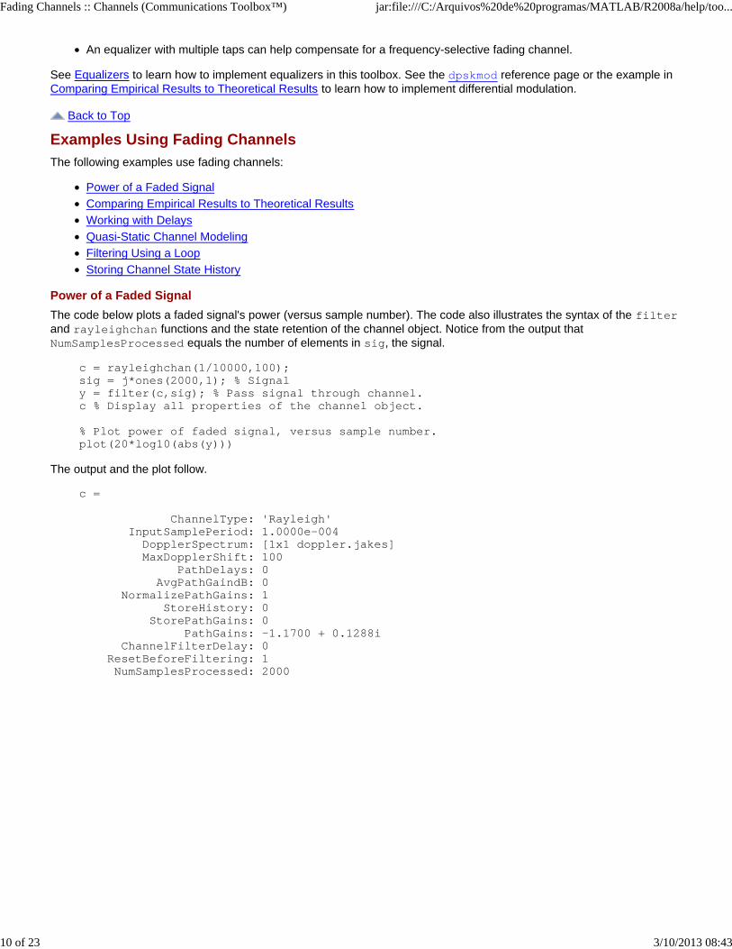
An equalizer with multiple taps can help compensate for a frequency-selective fading channel.

See Equalizers to learn how to implement equalizers in this toolbox. See the dpskmod reference page or the example in Comparing Empirical Results to Theoretical Results to learn how to implement differential modulation.

Back to Top

Examples Using Fading ChannelsThe following examples use fading channels:

Power of a Faded SignalComparing Empirical Results to Theoretical ResultsWorking with DelaysQuasi-Static Channel ModelingFiltering Using a LoopStoring Channel State History

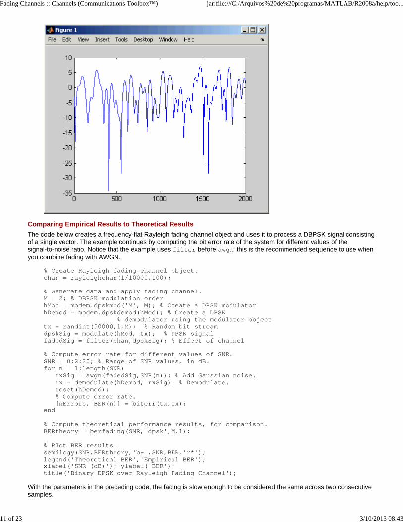
Power of a Faded SignalThe code below plots a faded signal's power (versus sample number). The code also illustrates the syntax of the filterand rayleighchan functions and the state retention of the channel object. Notice from the output thatNumSamplesProcessed equals the number of elements in sig, the signal.

c = rayleighchan(1/10000,100);sig = j*ones(2000,1); % Signaly = filter(c,sig); % Pass signal through channel.c % Display all properties of the channel object.

% Plot power of faded signal, versus sample number.plot(20*log10(abs(y)))

The output and the plot follow.

c = ChannelType: 'Rayleigh' InputSamplePeriod: 1.0000e-004 DopplerSpectrum: [1x1 doppler.jakes] MaxDopplerShift: 100 PathDelays: 0 AvgPathGaindB: 0 NormalizePathGains: 1 StoreHistory: 0 StorePathGains: 0 PathGains: -1.1700 + 0.1288i ChannelFilterDelay: 0 ResetBeforeFiltering: 1 NumSamplesProcessed: 2000


11 of 23 3/10/2013 08:43

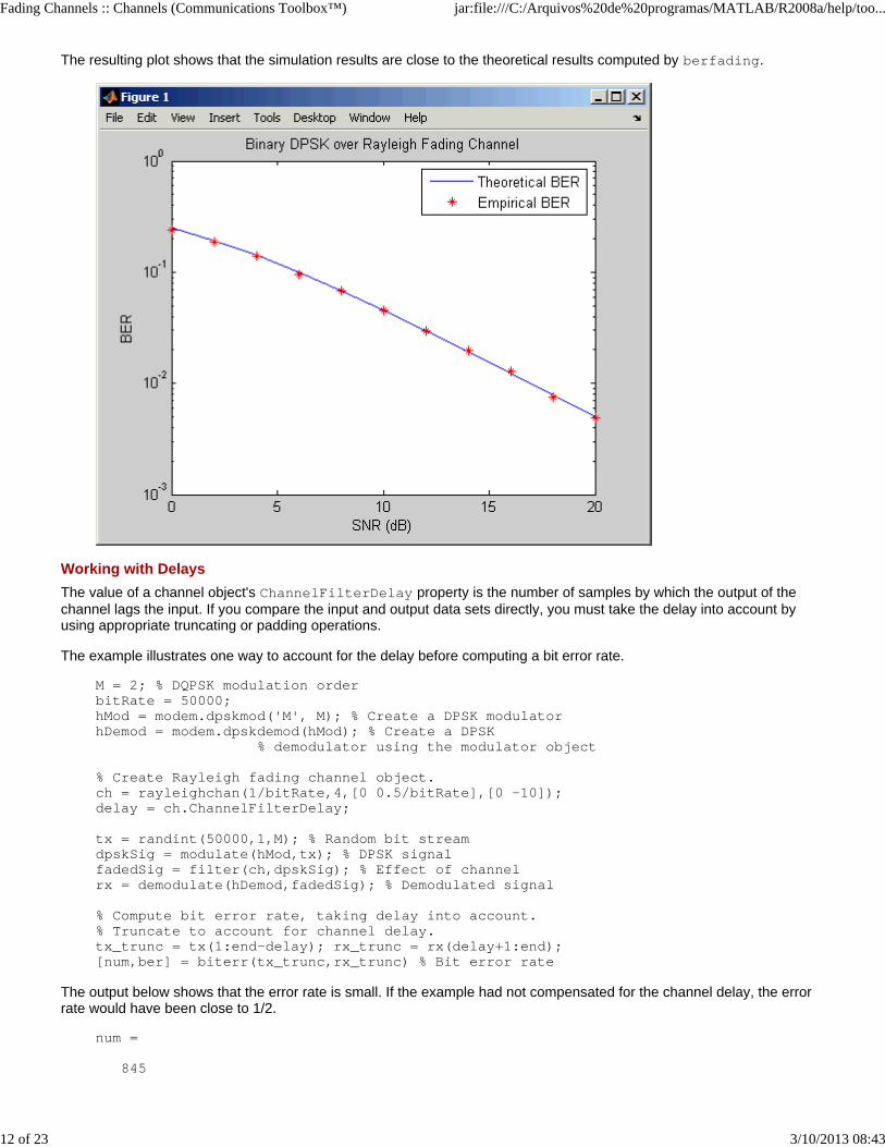
Comparing Empirical Results to Theoretical ResultsThe code below creates a frequency-flat Rayleigh fading channel object and uses it to process a DBPSK signal consistingof a single vector. The example continues by computing the bit error rate of the system for different values of thesignal-to-noise ratio. Notice that the example uses filter before awgn; this is the recommended sequence to use when you combine fading with AWGN.

% Create Rayleigh fading channel object.chan = rayleighchan(1/10000,100);

% Generate data and apply fading channel.M = 2; % DBPSK modulation orderhMod = modem.dpskmod('M', M); % Create a DPSK modulatorhDemod = modem.dpskdemod(hMod); % Create a DPSK % demodulator using the modulator objecttx = randint(50000,1,M); % Random bit streamdpskSig = modulate(hMod, tx); % DPSK signalfadedSig = filter(chan,dpskSig); % Effect of channel

% Compute error rate for different values of SNR.SNR = 0:2:20; % Range of SNR values, in dB.for n = 1:length(SNR) rxSig = awgn(fadedSig,SNR(n)); % Add Gaussian noise. rx = demodulate(hDemod, rxSig); % Demodulate. reset(hDemod); % Compute error rate. [nErrors, BER(n)] = biterr(tx,rx);end

% Compute theoretical performance results, for comparison.BERtheory = berfading(SNR,'dpsk',M,1);

% Plot BER results.semilogy(SNR,BERtheory,'b-',SNR,BER,'r*');legend('Theoretical BER','Empirical BER');xlabel('SNR (dB)'); ylabel('BER');title('Binary DPSK over Rayleigh Fading Channel');

With the parameters in the preceding code, the fading is slow enough to be considered the same across two consecutivesamples.


12 of 23 3/10/2013 08:43

The resulting plot shows that the simulation results are close to the theoretical results computed by berfading.

Working with DelaysThe value of a channel object's ChannelFilterDelay property is the number of samples by which the output of thechannel lags the input. If you compare the input and output data sets directly, you must take the delay into account byusing appropriate truncating or padding operations.

The example illustrates one way to account for the delay before computing a bit error rate.

M = 2; % DQPSK modulation orderbitRate = 50000;hMod = modem.dpskmod('M', M); % Create a DPSK modulatorhDemod = modem.dpskdemod(hMod); % Create a DPSK % demodulator using the modulator object

% Create Rayleigh fading channel object.ch = rayleighchan(1/bitRate,4,[0 0.5/bitRate],[0 -10]);delay = ch.ChannelFilterDelay;

tx = randint(50000,1,M); % Random bit streamdpskSig = modulate(hMod,tx); % DPSK signalfadedSig = filter(ch,dpskSig); % Effect of channelrx = demodulate(hDemod,fadedSig); % Demodulated signal

% Compute bit error rate, taking delay into account.% Truncate to account for channel delay.tx_trunc = tx(1:end-delay); rx_trunc = rx(delay+1:end);[num,ber] = biterr(tx_trunc,rx_trunc) % Bit error rate

The output below shows that the error rate is small. If the example had not compensated for the channel delay, the errorrate would have been close to 1/2.

num =

845


13 of 23 3/10/2013 08:43

ber =

0.0169

More Information About Working with Delays. The discussion in Effect of Delays on Recovery of Convolutionally Interleaved Data describes two typical ways to compensate for delays. Although the discussion there is about interleavingoperations instead of channel modeling, the techniques involving truncating and padding data are equally applicable tochannel modeling.

Quasi-Static Channel ModelingTypically, a path gain in a fading channel changes insignificantly over a period of 1/(100fd) seconds, where fd is the maximum Doppler shift. Because this period corresponds to a very large number of bits in many modern wireless dataapplications, assessing performance over a statistically significant range of fading entails simulating a prohibitively largeamount of data. Quasi-static channel modeling provides a more tractable approach, which you can implement using thesesteps:

Generate a random channel realization using a maximum Doppler shift of 0.1.Process some large number of bits.2.Compute error statistics.3.Repeat these steps many times to produce a distribution of the performance metric.4.

The example below illustrates the quasi-static channel modeling approach.

M = 4; % DQPSK modulation orderhMod = modem.dpskmod('M', M); % Create a DPSK modulatorhDemod = modem.dpskdemod(hMod); % Create a DPSK % demodulator using the modulator objectnumBits = 10000; % Each trial uses 10000 bits.numTrials = 20; % Number of BER computations

% Note: In reality, numTrials would be a large number% to get an accurate estimate of outage probabilities% or packet error rate.% Use 20 here just to make the example run more quickly.

% Create Rician channel object.chan = ricianchan; % Static channelchan.KFactor = 3; % Rician K-factor% Because chan.ResetBeforeFiltering is 1 by default,% FILTER resets the channel in each trial below.

% Compute error rate once for each independent trial.for n = 1:numTrials tx = randint(numBits,1,M); % Random bit stream dpskSig = modulate(hMod, tx); % DPSK signal fadedSig = filter(chan, dpskSig); % Effect of channel rxSig = awgn(fadedSig,20); % Add Gaussian noise. rx = demodulate(hDemod,rxSig); % Demodulate.

% Compute number of symbol errors. % Ignore first sample because of DPSK initial condition. nErrors(n) = symerr(tx(2:end),rx(2:end))endper = mean(nErrors > 0) % Proportion of packets that had errors

While the example runs, the Command Window displays the growing list of symbol error counts in the vector nErrors. It also displays the packet error rate at the end. The sample output below shows a final value of nErrors and omitsintermediate values. Your results might vary because of randomness in the example.

nErrors =

Columns 1 through 9

0 0 0 0 0 0 0 0 0


14 of 23 3/10/2013 08:43

Columns 10 through 18

0 0 0 0 7 0 0 0 0

Columns 19 through 20

0 216

per =

0.1000

More About the Quasi-Static Technique. As an example to show how the quasi-static channel modeling approach cansave computation, consider a wireless local area network (LAN) in which the carrier frequency is 2.4 GHz, mobile speed is1 m/s, and bit rate is 10 Mb/s. The following expression shows that the channel changes insignificantly over 12,500 bits:

A traditional Monte Carlo approach for computing the error rate of this system would entail simulating thousands of timesthe number of bits shown above, perhaps tens of millions of bits. By contrast, a quasi-static channel modeling approachwould simulate a few packets at each of about 100 locations to arrive at a spatial distribution of error rates. From thisdistribution one could determine, for example, how reliable the communication link is for a random location within theindoor space. If each simulation contains 5,000 bits, 100 simulations would process half a million bits in total. This issubstantially fewer bits compared to the traditional Monte Carlo approach.

Filtering Using a LoopThe section Configuring Channel Objects Based on Simulation Needs indicates how to invoke the filter function multiple times while maintaining continuity from one invocation to the next. The example below invokes filter within a loop and uses the small data sets from successive iterations to create an animated effect. The particular channel in thisexample is a Rayleigh fading channel with two discrete major paths.

% Set up parameters.M = 4; % QPSK modulation orderbitRate = 50000; % Data rate is 50 kb/s.numTrials = 125; % Number of iterations of loop

% Create Rayleigh fading channel object.ch = rayleighchan(1/bitRate,4,[0 2e-5],[0 -9]);% Indicate that FILTER should not reset the channel% in each iteration below.ch.ResetBeforeFiltering = 0;

% Initialize scatter plot.h = scatterplot(0);

% Apply channel in a loop, maintaining continuity.% Plot only the current data in each iteration.for n = 1:numTrials tx = randint(500,1,M); % Random bit stream pskSig = pskmod(tx,M); % PSK signal fadedSig = filter(ch, pskSig); % Effect of channel

% Plot the new data from this iteration. h = scatterplot(fadedSig,1,0,'b.',h); axis([-1.8 1.8 -1.8 1.8]) % Adjust axis limits. drawnow; % Refresh the image.end


15 of 23 3/10/2013 08:43

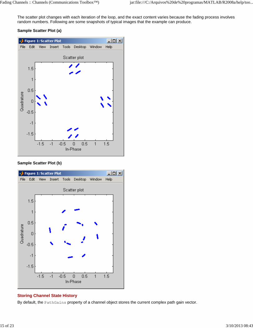
The scatter plot changes with each iteration of the loop, and the exact content varies because the fading process involvesrandom numbers. Following are some snapshots of typical images that the example can produce.

Sample Scatter Plot (a)

Sample Scatter Plot (b)

Storing Channel State HistoryBy default, the PathGains property of a channel object stores the current complex path gain vector.


16 of 23 3/10/2013 08:43

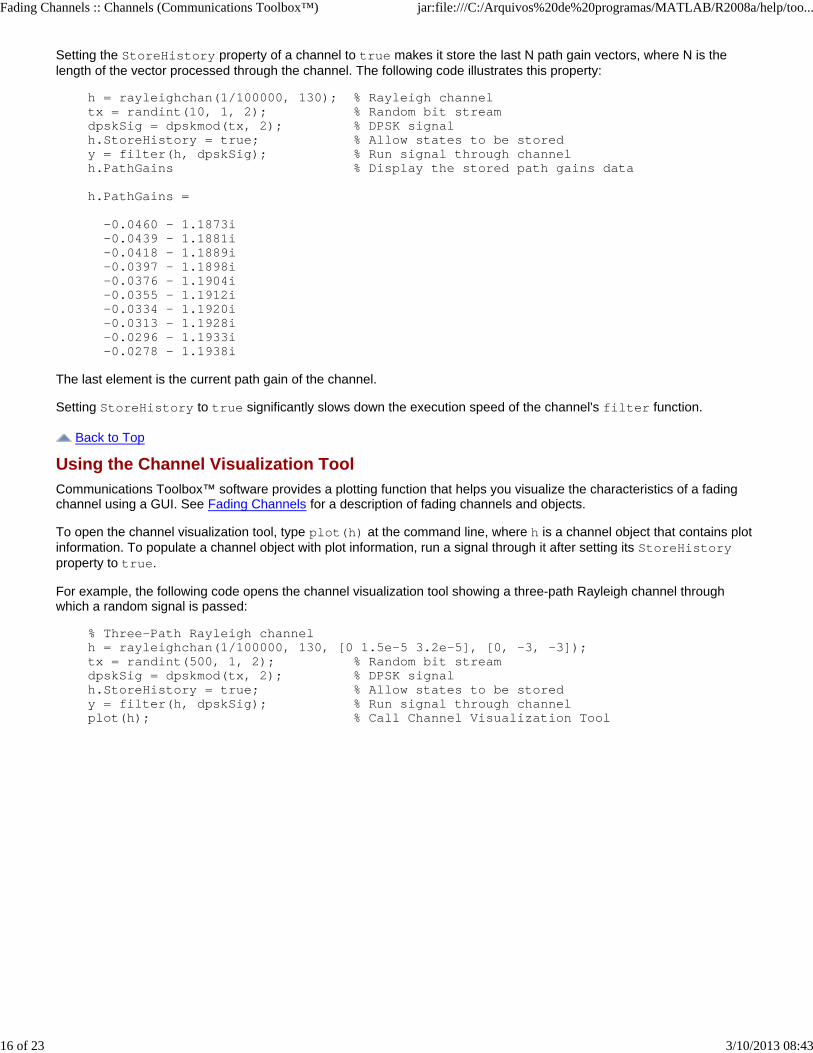
Setting the StoreHistory property of a channel to true makes it store the last N path gain vectors, where N is thelength of the vector processed through the channel. The following code illustrates this property:

h = rayleighchan(1/100000, 130); % Rayleigh channeltx = randint(10, 1, 2); % Random bit streamdpskSig = dpskmod(tx, 2); % DPSK signalh.StoreHistory = true; % Allow states to be storedy = filter(h, dpskSig); % Run signal through channelh.PathGains % Display the stored path gains data

h.PathGains =

-0.0460 - 1.1873i -0.0439 - 1.1881i -0.0418 - 1.1889i -0.0397 - 1.1898i -0.0376 - 1.1904i -0.0355 - 1.1912i -0.0334 - 1.1920i -0.0313 - 1.1928i -0.0296 - 1.1933i -0.0278 - 1.1938i

The last element is the current path gain of the channel.

Setting StoreHistory to true significantly slows down the execution speed of the channel's filter function.

Back to Top

Using the Channel Visualization ToolCommunications Toolbox™ software provides a plotting function that helps you visualize the characteristics of a fadingchannel using a GUI. See Fading Channels for a description of fading channels and objects.

To open the channel visualization tool, type plot(h) at the command line, where h is a channel object that contains plotinformation. To populate a channel object with plot information, run a signal through it after setting its StoreHistoryproperty to true.

For example, the following code opens the channel visualization tool showing a three-path Rayleigh channel throughwhich a random signal is passed:

% Three-Path Rayleigh channelh = rayleighchan(1/100000, 130, [0 1.5e-5 3.2e-5], [0, -3, -3]); tx = randint(500, 1, 2); % Random bit streamdpskSig = dpskmod(tx, 2); % DPSK signalh.StoreHistory = true; % Allow states to be storedy = filter(h, dpskSig); % Run signal through channelplot(h); % Call Channel Visualization Tool


17 of 23 3/10/2013 08:43

See Examples of Using the Channel Visualization Tool for the basic usage cases of the channel visualization tool.

This tool can also be accessed from Communications Blockset™ software.

Parts of the GUIThe Visualization pull-down menu allows you to choose the visualization method. See Visualization Options for details.

The Frame count counter shows the index of the current frame. It shows the number of frames processed by the filtermethod since the channel object was constructed or reset. A frame is a vector of M elements, interpreted to be Msuccessive samples that are uniformly spaced in time, with a sample period equal to that specified for the channel.

The Sample index slider control indicates which channel snapshot is currently being displayed, while the Pause button pauses a running animation until you click it again. The slider control and Pause button apply to all visualizations exceptthe Doppler Spectrum.

The Animation pull-down menu allows you to select how you want to display the channel snapshots within each frame.Setting this to Slow makes the tool show channel snapshots in succession, starting at the sample set by the Sample index slider control. Selecting Medium or Fast makes the tool show fewer uniformly spaced snapshots, allowing you togo through the channel snapshots more rapidly. Selecting Interframe only (the default selection) prevents automatic animation of snapshots within the same frame. The Animation menu applies to all visualizations except the DopplerSpectrum.

Visualization OptionsThe channel visualization tool plots the characteristics of a filter in various ways. Simply choose the visualization methodfrom the Visualization menu, and the plot updates itself automatically.

The following visualization methods are currently available:

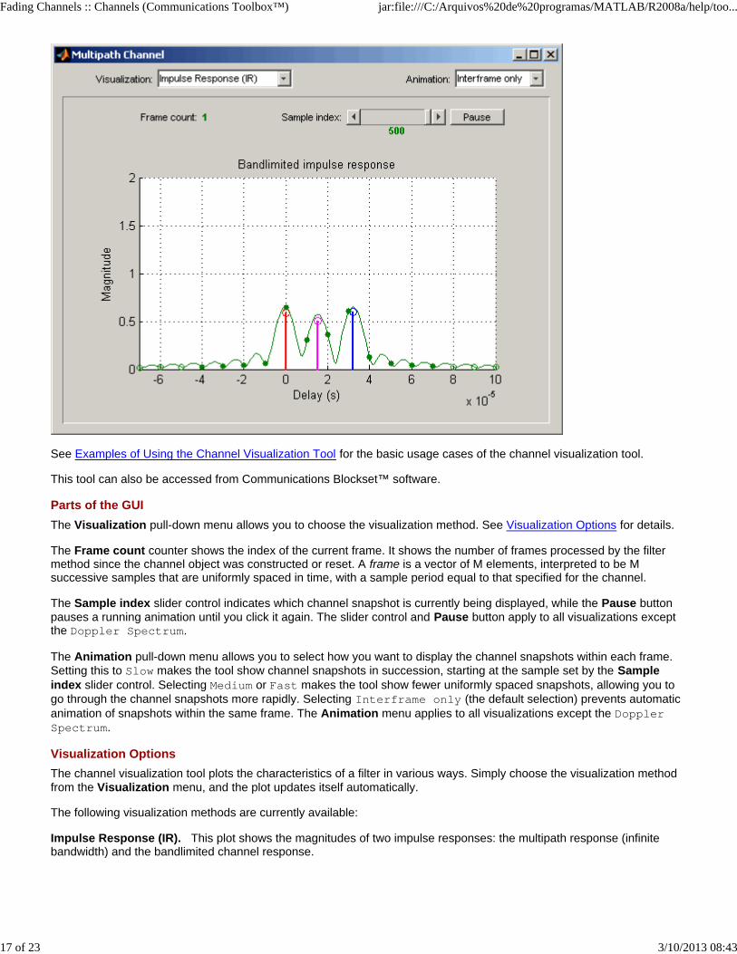
Impulse Response (IR). This plot shows the magnitudes of two impulse responses: the multipath response (infinitebandwidth) and the bandlimited channel response.


18 of 23 3/10/2013 08:43

The multipath response is represented by stems, each corresponding to one multipath component. The component withthe smallest delay value is shown in red, and the component with the largest delay value is shown in blue. Componentswith intermediate delay values are shades between red and blue, becoming more blue for larger delays.

The bandlimited channel response is represented by the green curve. This response is the result of convolving themultipath impulse response, described above, with a sinc pulse of period, T, equal to the input signal's sample period.

The solid green circles represent the channel filter response sampled at rate 1/T. The output of the channel filter is theconvolution of the input signal (sampled at rate 1/T) with this discrete-time FIR channel filter response. For computationalspeed, the response is truncated.

The hollow green circles represent sample values not captured in the channel filter response that is used for processingthe input signal.

Note that these impulse responses vary over time. You can use the slider to visualize how the impulse response changesover time for the current frame (i.e., input signal vector over time).

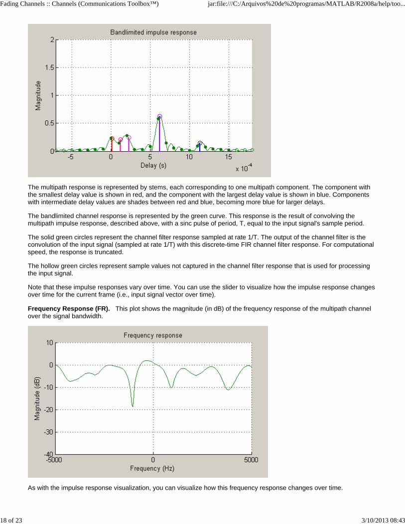
Frequency Response (FR). This plot shows the magnitude (in dB) of the frequency response of the multipath channelover the signal bandwidth.

As with the impulse response visualization, you can visualize how this frequency response changes over time.


19 of 23 3/10/2013 08:43

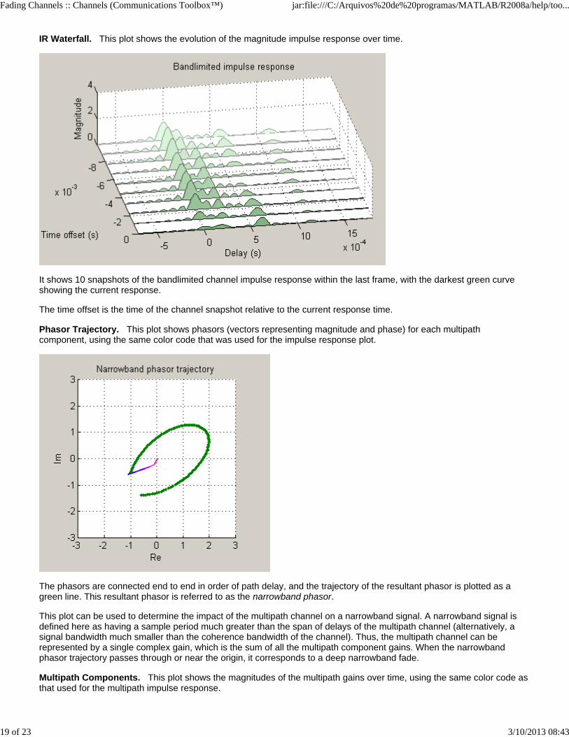
IR Waterfall. This plot shows the evolution of the magnitude impulse response over time.

It shows 10 snapshots of the bandlimited channel impulse response within the last frame, with the darkest green curveshowing the current response.

The time offset is the time of the channel snapshot relative to the current response time.

Phasor Trajectory. This plot shows phasors (vectors representing magnitude and phase) for each multipathcomponent, using the same color code that was used for the impulse response plot.

The phasors are connected end to end in order of path delay, and the trajectory of the resultant phasor is plotted as agreen line. This resultant phasor is referred to as the narrowband phasor.

This plot can be used to determine the impact of the multipath channel on a narrowband signal. A narrowband signal isdefined here as having a sample period much greater than the span of delays of the multipath channel (alternatively, asignal bandwidth much smaller than the coherence bandwidth of the channel). Thus, the multipath channel can berepresented by a single complex gain, which is the sum of all the multipath component gains. When the narrowbandphasor trajectory passes through or near the origin, it corresponds to a deep narrowband fade.

Multipath Components. This plot shows the magnitudes of the multipath gains over time, using the same color code asthat used for the multipath impulse response.


20 of 23 3/10/2013 08:43

The triangle marker and vertical dashed line represent the start of the current frame. If a frame has been processedpreviously, its multipath gains may also be displayed.

Multipath Gain. This plot shows the collective gains for the multipath channel for three signal bandwidths.

A collective gain is the sum of component magnitudes, as explained in the following:

Narrowband (magenta dots): This is the magnitude of the narrowband phasor in the above trajectory plot. Thiscurve is sometimes referred to as the narrowband fading envelope.Current signal bandwidth (dashed blue line): This is the sum of the magnitudes of the channel filter impulseresponse samples (the solid green dots in the impulse response plot). This curve represents the maximum signalenergy that can be captured using a RAKE receiver. Its value (or metrics, such as theoretical BER, derived from it)is sometimes referred to as the matched filter bound.Infinite bandwidth (solid red line): This is the sum of the magnitudes of the multipath component gains.

In general, the variability of this multipath gain, or of the signal fading, decreases as signal bandwidth is increased,because multipath components become more resolvable. If the signal bandwidth curve roughly follows the narrowbandcurve, you might describe the signal as narrowband. If the signal bandwidth curve roughly follows the infinite bandwidthcurve, you might describe the signal as wideband. With the right receiver, a wideband signal exploits the path diversityinherent in a multipath channel.


21 of 23 3/10/2013 08:43

Doppler Spectrum. This plot shows up to two Doppler spectra.

The first Doppler spectrum, represented by the dashed red line, is a theoretical spectrum based on the Doppler filterresponse used in the multipath channel model. In the preceding plot, the theoretical Doppler spectrum used for themultipath channel model is known as the Jakes spectrum. Note that the plotted Doppler spectrum is normalized to have atotal power of 1. This Doppler spectrum is used to determine a Doppler filter response. For practical purposes, theDoppler filter response is truncated, which has the effect of modifying the Doppler spectrum, as shown in the plot.

The second Doppler spectrum, represented by the blue dots, is determined by measuring the power spectrum of themultipath fading channel as the model generates path gains. This measurement is meaningful only after enough pathgains have been generated. The title above the plot reports how many samples need to be processed through thechannel before either the first Doppler spectrum or an updated spectrum can be plotted.

The Path Number edit box allows you to visualize the Doppler spectrum of the specified path. The value entered in thisbox must be a valid path number, i.e., between 1 and the length of the PathDelays vector property. Once you changethe value of this field, the new Doppler spectrum will appear as soon as the processing of the current frame has ended.

If the measured Doppler spectrum is a good approximation of the theoretical Doppler spectrum, the multipath channelmodel has generated enough fading gains to yield a reasonable representation of the channel statistics. For instance, ifyou want to determine the average BER of a communications link with a multipath channel and you want a statisticallyaccurate measure of this average, you may want to ensure that the channel has processed enough samples to yield atleast one Doppler spectrum measurement.

It is possible that a multipath channel (e.g., a Rician channel) can have both specular (line-of-sight) and diffusecomponents. In such a case, the Doppler spectrum would have both a line component and a wideband component. Thechannel visualization tool only shows the wideband component for the Doppler spectrum.

Unlike other visualizations, the Doppler spectrum visualization does not support animation. Because there is no intraframedata to plot, the visualization tool only updates the channel statistics at the end of each frame and therefore cannot pausein the middle of a frame. If you switch to the Doppler spectrum visualization from a different visualization that is in pausemode, the Pause button is subsequently disabled. Disabling pause avoids interaction problems between the Dopplerspectrum visualization and other animation-style visualizations.

Scattering Function. This plot shows the Doppler spectra of each path versus the path delays, using the same colorcode as that used for the multipath impulse response.


22 of 23 3/10/2013 08:43

The principle of operation of the Scattering Function plot is similar to that of the Doppler Spectrum plot. The maindifference is that the Doppler spectra on this plot are not normalized as they are on the Doppler Spectrum plot, in order tobetter visualize the power delay profile.

Composite Plots. Several composite plots are also available. These are chosen by selecting the following from theVisualization pull-down menu:

IR and FR for impulse response and frequency response plots.Components and Gain for multipath components and multipath gain plots.Components and IR for multipath components and impulse response plots.Components, IR, and Phasor for multipath components, impulse response, and phasor trajectory plots.

Examples of Using the Channel Visualization ToolHere are two examples that show how you might interact with the GUI.

Visualizing Samples Within a FrameAnimating Snapshots Across Frames

Visualizing Samples Within a Frame. This example shows how to visualize samples within a frame through animation.The following lines of code create a Rayleigh channel and open the channel visualization tool:

% Create a fast fading channelh = rayleighchan(1e-4, 100, [0 1.1e-4], [0 0]);

h.StoreHistory = 1; % Allow states to be storedy = filter(h, ones(100,1)); % Process samples through channelplot(h); % Open channel visualization tool

After selecting a visualization option and a speed in the Animation menu, move the Sample index slider control all the way to the left and click Resume. The slider control moves by itself during animation. The sample index incrementsautomatically to show which snapshot you are visualizing.

You can also move the slider control and glance through the samples of the frame as you like.

Animating Snapshots Across Frames. This example shows how to animate snapshots across frames. The followinglines of code call the filter and plot methods within a loop to accomplish this:

Ts = 1e-4; % Sample period (s)fd = 100; % Maximum Doppler shift

% Path delay and gainstau = [0.1 1.2 2.3 6.2 11.3]*Ts;


23 of 23 3/10/2013 08:43

PdB = linspace(0, -10, length(tau)) - length(tau)/20;

nTrials = 10000; % Number of trialsN = 100; % Number of samples per frame

h = rayleighchan(Ts, fd, tau, PdB); % Create channel objecth.NormalizePathGains = false;h.ResetBeforeFiltering = false;h.StoreHistory = 1;h % Show channel object

% Channel fading simulationfor trial = 1:nTrials x = randint(10000, 1, 4); dpskSig = dpskmod(x, 4); y = filter(h, dpskSig); plot(h); % The line below returns control to the command line in case % the GUI is closed while this program is still running if isempty(findobj('name', 'Multipath Channel')), break; end;end

While the animation is running, you can move the slider control and change the sample index (which also makes theanimation pause). After clicking Resume, the plot continues to animate.

The property ResetBeforeFiltering needs to be set to false so that the state information in the channel is not resetafter the processing of each frame.

Back to Top Provide feedback about this page

AWGN Channel Binary Symmetric Channel

© 1984-2008 The MathWorks, Inc. • Terms of Use • Patents • Trademarks • Acknowledgments

Documents

Provide feedback about this page Fading Channelsmdoniak/CDI_20705/Fading%20... · Fading Channels :: Channels (Communications Toolbox™) jar: ... In the example below, entering c1