Embed Size (px)
Citation preview
Digital CommunicationsChapter 13 Fading Channels I: Characterization and Signaling
Po-Ning Chen, Professor
Institute of Communications EngineeringNational Chiao-Tung University, Taiwan
Digital Communications: Chapter 13 Ver 2016.05.04 Po-Ning Chen 1 / 114
13.1 Characterization of fadingmultipath channels
Digital Communications: Chapter 13 Ver 2016.05.04 Po-Ning Chen 2 / 114
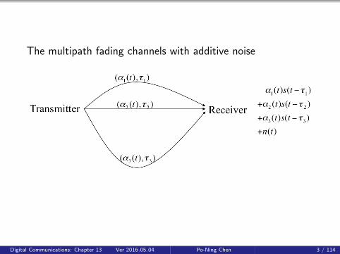
The multipath fading channels with additive noise
Digital Communications: Chapter 13 Ver 2016.05.04 Po-Ning Chen 3 / 114

Time spread phenomenon of multipath channels(Unpredictable) Time-variant factors
Delay
Number of spreads
Size of the receive pulses
Digital Communications: Chapter 13 Ver 2016.05.04 Po-Ning Chen 4 / 114
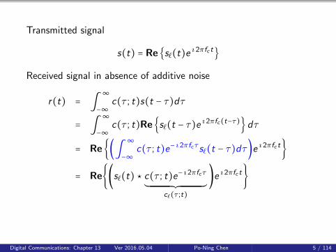
Transmitted signal
s(t) = Re{s`(t)e ı2πfc t}
Received signal in absence of additive noise
r(t) = ∫∞
−∞c(τ ; t)s(t − τ)dτ
= ∫∞
−∞c(τ ; t)Re{s`(t − τ)e ı2πfc(t−τ)}dτ
= Re{(∫∞
−∞c(τ ; t)e− ı2πfcτ s`(t − τ)dτ)e ı2πfc t}
= Re{(s`(t) ⋆ c(τ ; t)e− ı2πfcτ
´¹¹¹¹¹¹¹¹¹¹¹¹¹¹¹¹¹¹¹¹¹¹¹¹¹¹¹¹¹¹¹¹¹¹¹¹¸¹¹¹¹¹¹¹¹¹¹¹¹¹¹¹¹¹¹¹¹¹¹¹¹¹¹¹¹¹¹¹¹¹¹¹¹¹¶c`(τ ;t)
)e ı2πfc t}
Digital Communications: Chapter 13 Ver 2016.05.04 Po-Ning Chen 5 / 114
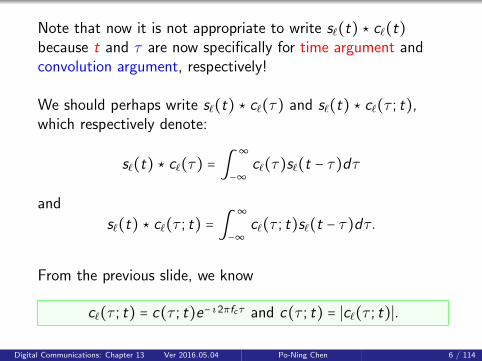
Note that now it is not appropriate to write s`(t) ⋆ c`(t)because t and τ are now specifically for time argument andconvolution argument, respectively!
We should perhaps write s`(t) ⋆ c`(τ) and s`(t) ⋆ c`(τ ; t),which respectively denote:
s`(t) ⋆ c`(τ) = ∫∞
−∞c`(τ)s`(t − τ)dτ
and
s`(t) ⋆ c`(τ ; t) = ∫∞
−∞c`(τ ; t)s`(t − τ)dτ.
From the previous slide, we know
c`(τ ; t) = c(τ ; t)e− ı2πfcτ and c(τ ; t) = ∣c`(τ ; t)∣.
Digital Communications: Chapter 13 Ver 2016.05.04 Po-Ning Chen 6 / 114
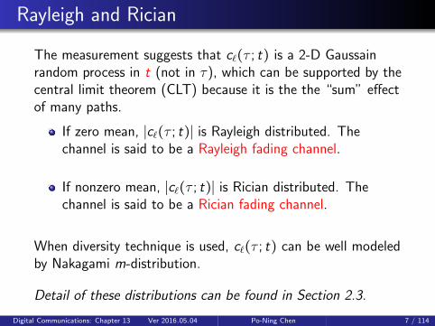
Rayleigh and Rician
The measurement suggests that c`(τ ; t) is a 2-D Gaussainrandom process in t (not in τ), which can be supported by thecentral limit theorem (CLT) because it is the the “sum” effectof many paths.
If zero mean, ∣c`(τ ; t)∣ is Rayleigh distributed. Thechannel is said to be a Rayleigh fading channel.
If nonzero mean, ∣c`(τ ; t)∣ is Rician distributed. Thechannel is said to be a Rician fading channel.
When diversity technique is used, c`(τ ; t) can be well modeledby Nakagami m-distribution.
Detail of these distributions can be found in Section 2.3.
Digital Communications: Chapter 13 Ver 2016.05.04 Po-Ning Chen 7 / 114
13.1-1 Channel correlationfunctions and power spectra
Digital Communications: Chapter 13 Ver 2016.05.04 Po-Ning Chen 8 / 114
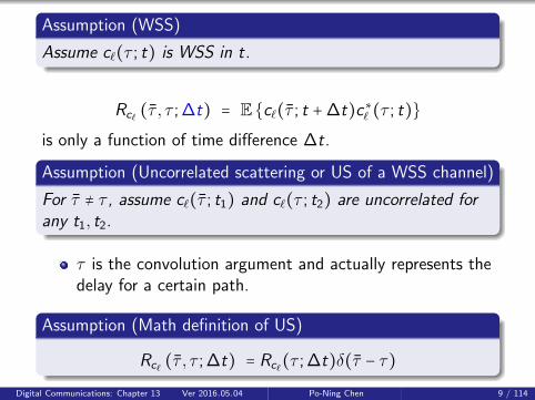
Assumption (WSS)
Assume c`(τ ; t) is WSS in t.
Rc` (τ , τ ; ∆t) = E{c`(τ ; t +∆t)c∗` (τ ; t)}is only a function of time difference ∆t.
Assumption (Uncorrelated scattering or US of a WSS channel)
For τ ≠ τ , assume c`(τ ; t1) and c`(τ ; t2) are uncorrelated forany t1, t2.
τ is the convolution argument and actually represents thedelay for a certain path.
Assumption (Math definition of US)
Rc` (τ , τ ; ∆t) = Rc`(τ ; ∆t)δ(τ − τ)
Digital Communications: Chapter 13 Ver 2016.05.04 Po-Ning Chen 9 / 114
Discussions
It may appear “unnatural” to “define” the autocorrelationfunction of a channel impulse response using the Diracdelta function.
However, we have already learned that τ is theconvolution argument, and δ(τ) is the impulse responseof the identity channel. This somehow hints that there isa connection between “channel impulse response” and“Dirac delta function.”
Recall that a WSS white (noise) process z(τ) is definedbased on
Rz(∆τ) = E[z(τ +∆τ)z∗(τ)] = N0
2δ(∆τ).
Digital Communications: Chapter 13 Ver 2016.05.04 Po-Ning Chen 10 / 114

Discussions (Continued)
We can extensively view that the autocorrelation function of a2-dimensional WSS white noise z(τ ; t) is defined as
E[z(τ +∆τ ; t1)z∗(τ ; t2)] =N0(t1, t2)
2δ(∆τ).
US indicates that the accumulated power correlation from allother paths is essentially zero!
Some researchers interpret “US” as “zero-correlationscattering.” So, from this, they don’t interpret it as
E[z(τ+∆τ ; t1)z∗(τ ; t2)]uncorrelated= E[z(τ+∆τ ; t1)]E[z∗(τ ; t2)] = 0,
which requires “zero-mean” assumption but simply say
E[z(τ +∆τ ; t1)z∗(τ ; t2)] = 0 when ∆τ ≠ 0.
Digital Communications: Chapter 13 Ver 2016.05.04 Po-Ning Chen 11 / 114
Multipath intensity profile of a US-WSS channel
The multipath intensity profile or delay powerspectrum for a US-WSS multipath fading channel isgiven by:
Rc` (τ) = Rc` (τ ; ∆t = 0) .
It can be interpreted as the average signal powerremained after delay τ .
Digital Communications: Chapter 13 Ver 2016.05.04 Po-Ning Chen 12 / 114
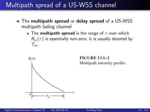
Multipath spread of a US-WSS channel
The multipath spread or delay spread of a US-WSSmultipath fading channel
The multipath spread is the range of τ over whichRc`(τ) is essentially non-zero; it is usually denoted byTm.
Digital Communications: Chapter 13 Ver 2016.05.04 Po-Ning Chen 13 / 114
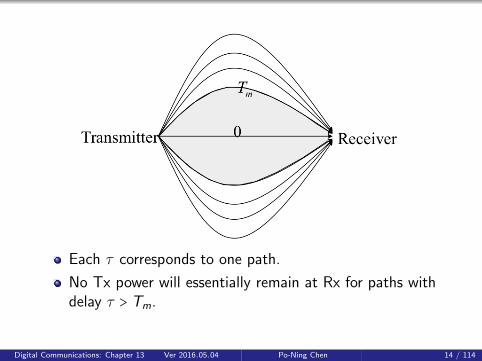
Each τ corresponds to one path.
No Tx power will essentially remain at Rx for paths withdelay τ > Tm.
Digital Communications: Chapter 13 Ver 2016.05.04 Po-Ning Chen 14 / 114
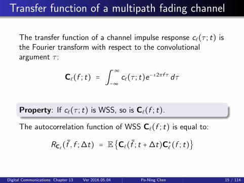
Transfer function of a multipath fading channel
The transfer function of a channel impulse response c`(τ ; t) isthe Fourier transform with respect to the convolutionalargument τ :
C`(f ; t) = ∫∞
−∞c`(τ ; t)e− ı2πf τ dτ
Property: If c`(τ ; t) is WSS, so is C`(f ; t).
The autocorrelation function of WSS C`(f ; t) is equal to:
RC`(f , f ; ∆t) = E{C`(f ; t +∆t)C∗` (f ; t)}
Digital Communications: Chapter 13 Ver 2016.05.04 Po-Ning Chen 15 / 114

With an additional US assumption,
RC`(f , f ; ∆t)= E{C`(f ; t +∆t)C∗
` (f ; t)}
= E{∫∞
−∞c`(τ ; t +∆t)e− ı2πf τ d τ ∫
∞
−∞c∗` (τ ; t)e ı2πf τ dτ}
= ∫∞
−∞∫
∞
−∞Rc`(τ ; ∆t)δ(τ − τ)e ı2π(f τ−f τ) dτd τ
= ∫∞
−∞Rc` (τ ; ∆t) e− ı2π(f −f )τ dτ
= RC` (∆f ; ∆t), where ∆f = f − f .
For a US-WSS multipath fading channel,
RC`(∆f ; ∆t) = E{C`(f +∆f ; t +∆t)C∗` (f ; t)}
This is often called spaced-frequency, spaced-timecorrelation function of a US-WSS channel.
Digital Communications: Chapter 13 Ver 2016.05.04 Po-Ning Chen 16 / 114
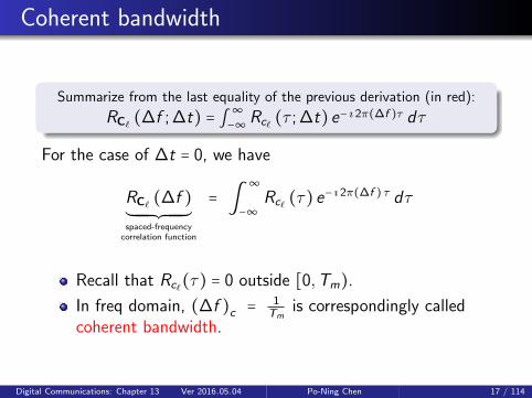
Coherent bandwidth
Summarize from the last equality of the previous derivation (in red):
RC` (∆f ; ∆t) = ∫∞−∞Rc` (τ ; ∆t) e− ı2π(∆f )τ dτ
For the case of ∆t = 0, we have
RC` (∆f )´¹¹¹¹¹¹¹¹¹¹¹¹¹¹¹¸¹¹¹¹¹¹¹¹¹¹¹¹¹¹¹¶spaced-frequency
correlation function
= ∫∞
−∞Rc` (τ) e− ı2π(∆f ) τ dτ
Recall that Rc`(τ) = 0 outside [0,Tm).
In freq domain, (∆f )c = 1Tm
is correspondingly calledcoherent bandwidth.
Digital Communications: Chapter 13 Ver 2016.05.04 Po-Ning Chen 17 / 114

Digital Communications: Chapter 13 Ver 2016.05.04 Po-Ning Chen 18 / 114
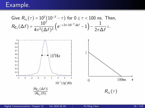
Example.
Give Rc`(τ) = 107(10−7 − τ) for 0 ≤ τ < 100 ns. Then,
RC`(∆f ) = 107
4π2(∆f )2(e− ı2π⋅10−7⋅∆f − 1) − 1
2π∆fı .
∣RC`(∆f )∣
∣RC`(0)∣ Rc`(τ)
Digital Communications: Chapter 13 Ver 2016.05.04 Po-Ning Chen 19 / 114
Coherent bandwidth
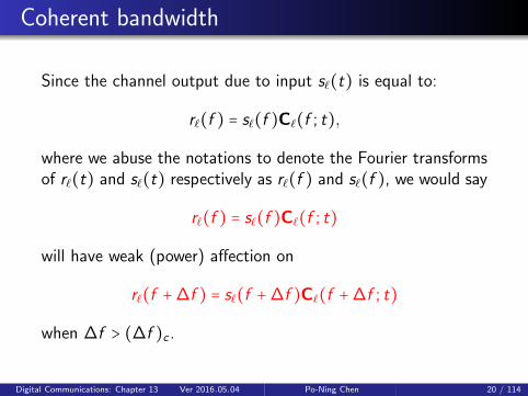
Since the channel output due to input s`(t) is equal to:
r`(f ) = s`(f )C`(f ; t),
where we abuse the notations to denote the Fourier transformsof r`(t) and s`(t) respectively as r`(f ) and s`(f ), we would say
r`(f ) = s`(f )C`(f ; t)
will have weak (power) affection on
r`(f +∆f ) = s`(f +∆f )C`(f +∆f ; t)
when ∆f > (∆f )c .
Digital Communications: Chapter 13 Ver 2016.05.04 Po-Ning Chen 20 / 114
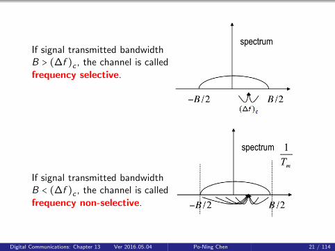
If signal transmitted bandwidthB > (∆f )c , the channel is calledfrequency selective.
If signal transmitted bandwidthB < (∆f )c , the channel is calledfrequency non-selective.
Digital Communications: Chapter 13 Ver 2016.05.04 Po-Ning Chen 21 / 114
For frequency selective channels, the signal shape is moreseverely distorted than that of frequency non-selectivechannels.
Criterion for frequency selectivity:
B > (∆f )c ⇔ 1
T> 1
Tm
⇔ T < Tm.
Digital Communications: Chapter 13 Ver 2016.05.04 Po-Ning Chen 22 / 114
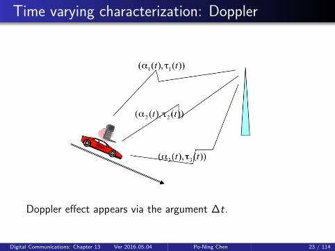
Time varying characterization: Doppler
Doppler effect appears via the argument ∆t.
Digital Communications: Chapter 13 Ver 2016.05.04 Po-Ning Chen 23 / 114
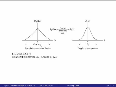
Doppler power spectrum of a US-WSS channel
The Doppler power spectrum is
SC`(λ) = ∫∞
−∞RC`(∆f = 0; ∆t)e− ı2πλ(∆t)d(∆t),
where λ is referred to as the Doppler frequency.
Bd = Doppler spread is the range such that SC`(λ) isessentially zero.
(∆t)c = 1Bd
is called the coherent time.
If symbol period T > (∆t)c , the channel is classified asFast Fading.
I.e., channel statistics changes within one symbol!
If symbol period T < (∆t)c , the channel is classified asSlow Fading.
Digital Communications: Chapter 13 Ver 2016.05.04 Po-Ning Chen 24 / 114
Digital Communications: Chapter 13 Ver 2016.05.04 Po-Ning Chen 25 / 114
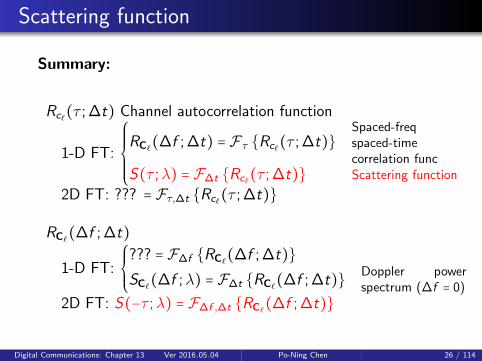
Scattering function
Summary:
Rc`(τ ; ∆t) Channel autocorrelation function
1-D FT:
⎧⎪⎪⎪⎪⎨⎪⎪⎪⎪⎩
RC`(∆f ; ∆t) = F τ {Rc`(τ ; ∆t)}Spaced-freqspaced-timecorrelation func
S(τ ;λ) = F∆t {Rc`(τ ; ∆t)} Scattering function
2D FT: ??? = Fτ,∆t {Rc`(τ ; ∆t)}
RC`(∆f ; ∆t)
1-D FT:
⎧⎪⎪⎨⎪⎪⎩
??? = F∆f {RC`(∆f ; ∆t)}SC`(∆f ;λ) = F∆t {RC`(∆f ; ∆t)} Doppler power
spectrum (∆f = 0)
2D FT: S(−τ ;λ) = F∆f ,∆t {RC`(∆f ; ∆t)}
Digital Communications: Chapter 13 Ver 2016.05.04 Po-Ning Chen 26 / 114
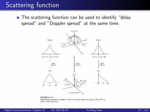
Scattering function
The scattering function can be used to identify “delayspread” and ”Doppler spread” at the same time.
Digital Communications: Chapter 13 Ver 2016.05.04 Po-Ning Chen 27 / 114

Example. Medium-range tropospheric scatter
channel
Digital Communications: Chapter 13 Ver 2016.05.04 Po-Ning Chen 28 / 114
Example study of delay spread
The median delay spread is the 50% value, meaning that50% of all channels has a delay spread that is lower than themedian value. Clearly, the median value is not so interestingfor designing a wireless link, because you want to guaranteethat the link works for at least 90% or 99% of all channels.Therefore the second column gives the measured maximumdelay spread values. The reason to use maximum delayspread instead of a 90% or 99% value is that many papersonly mention the maximum value. From the papers that dopresent cumulative distribution functions of their measureddelay spreads, it can be deduced that the 99% value is only afew percent smaller than the maximum delay spread.
Digital Communications: Chapter 13 Ver 2016.05.04 Po-Ning Chen 29 / 114
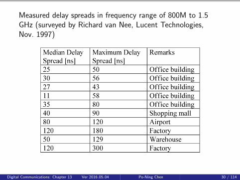
Measured delay spreads in frequency range of 800M to 1.5GHz (surveyed by Richard van Nee, Lucent Technologies,Nov. 1997)
Digital Communications: Chapter 13 Ver 2016.05.04 Po-Ning Chen 30 / 114
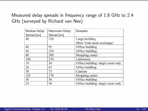
Measured delay spreads in frequency range of 1.8 GHz to 2.4GHz (surveyed by Richard van Nee)
Digital Communications: Chapter 13 Ver 2016.05.04 Po-Ning Chen 31 / 114
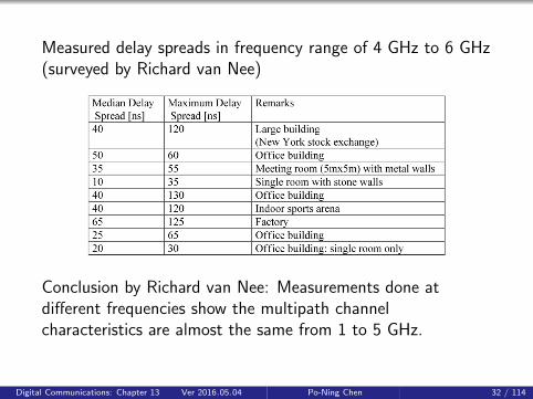
Measured delay spreads in frequency range of 4 GHz to 6 GHz(surveyed by Richard van Nee)
Conclusion by Richard van Nee: Measurements done atdifferent frequencies show the multipath channelcharacteristics are almost the same from 1 to 5 GHz.
Digital Communications: Chapter 13 Ver 2016.05.04 Po-Ning Chen 32 / 114

Jakes’ model: Example 13.1-3
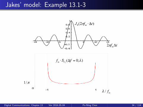
Jakes’ modelA widely used model for Doppler power spectrum is theso-called Jakes’ model (Jakes, 1974)
RC`(∆t) = J0(2πfm ⋅∆t)and
SC`(λ) =⎧⎪⎪⎨⎪⎪⎩
1πfm
1√1−(λ/fm)2
, ∣λ∣ ≤ fm
0, otherwise
where
⎧⎪⎪⎪⎪⎪⎪⎪⎪⎪⎪⎪⎪⎪⎨⎪⎪⎪⎪⎪⎪⎪⎪⎪⎪⎪⎪⎪⎩
fm = (v/c)fc is the maximum Doppler shift
v is the vehicle speed (m/s)
c is the light speed (3 × 10⁸ m/s)
fc is the carrier frequency
J0(⋅) is the zero-order Bessel function
of the first kind.
Digital Communications: Chapter 13 Ver 2016.05.04 Po-Ning Chen 33 / 114
Jakes’ model: Example 13.1-3
Digital Communications: Chapter 13 Ver 2016.05.04 Po-Ning Chen 34 / 114
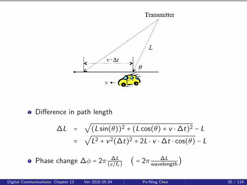
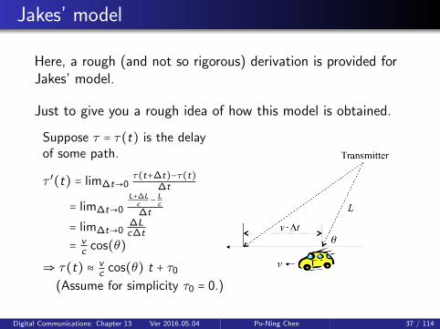
Difference in path length
∆L =√
(L sin(θ))2 + (L cos(θ) + v ⋅∆t)2 − L
=√L2 + v2(∆t)2 + 2L ⋅ v ⋅∆t ⋅ cos(θ) − L
Phase change ∆φ = 2π ∆L(c/fc) ( = 2π ∆L
wavelength)
Digital Communications: Chapter 13 Ver 2016.05.04 Po-Ning Chen 35 / 114
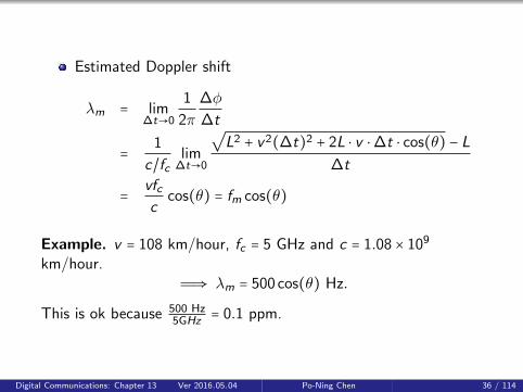
Estimated Doppler shift
λm = lim∆t→0
1
2π
∆φ
∆t
= 1
c/fclim
∆t→0
√L2 + v2(∆t)2 + 2L ⋅ v ⋅∆t ⋅ cos(θ) − L
∆t
= vfcc
cos(θ) = fm cos(θ)
Example. v = 108 km/hour, fc = 5 GHz and c = 1.08 × 10⁹
km/hour.Ô⇒ λm = 500 cos(θ) Hz.
This is ok because 500 Hz5GHz = 0.1 ppm.
Digital Communications: Chapter 13 Ver 2016.05.04 Po-Ning Chen 36 / 114
Jakes’ model
Here, a rough (and not so rigorous) derivation is provided forJakes’ model.
Just to give you a rough idea of how this model is obtained.
Suppose τ = τ(t) is the delayof some path.
τ ′(t) = lim∆t→0τ(t+∆t)−τ(t)
∆t
= lim∆t→0
L+∆Lc
− Lc
∆t
= lim∆t→0∆Lc∆t
= vc cos(θ)
⇒ τ(t) ≈ vc cos(θ) t + τ0
(Assume for simplicity τ0 = 0.)
Digital Communications: Chapter 13 Ver 2016.05.04 Po-Ning Chen 37 / 114
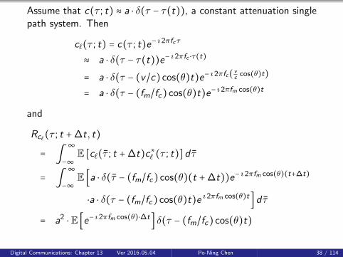
Assume that c(τ ; t) ≈ a ⋅ δ(τ − τ(t)), a constant attenuation singlepath system. Then
c`(τ ; t) = c(τ ; t)e− ı2πfcτ
≈ a ⋅ δ(τ − τ(t))e− ı2πfc ⋅τ(t)
= a ⋅ δ(τ − (v/c) cos(θ)t)e− ı2πfc( vc
cos(θ)t)
= a ⋅ δ(τ − (fm/fc) cos(θ)t)e− ı2πfm cos(θ)t
and
Rc`(τ ; t +∆t, t)
= ∫∞
−∞E [c`(τ ; t +∆t)c∗` (τ ; t)]d τ
= ∫∞
−∞E [a ⋅ δ(τ − (fm/fc) cos(θ)(t +∆t))e− ı2πfm cos(θ)(t+∆t)
⋅a ⋅ δ(τ − (fm/fc) cos(θ)t)e ı2πfm cos(θ)t]d τ
= a2 ⋅E [e− ı2πfm cos(θ)⋅∆t] δ(τ − (fm/fc) cos(θ)t)
Digital Communications: Chapter 13 Ver 2016.05.04 Po-Ning Chen 38 / 114
RC`(∆f = 0; t +∆t, t) ( = ∫∞
−∞Rc`(τ ; t +∆t, t)e ı2π(∆f )τdτ)
= ∫∞
−∞Rc`(τ ; t +∆t, t)dτ
= ∫∞
−∞a2 ⋅E [e− ı2πfm cos(θ)⋅∆t] δ(τ − (fm/fc) cos(θ)t)dτ
= a2 ⋅E [e− ı2πfm cos(θ)⋅∆t]
= J0(2πfm ⋅∆t) ( = RC`(∆f = 0; ∆t))
where the last step is valid if θ uniformly distributed over [−π,π),
and a = 1.
Digital Communications: Chapter 13 Ver 2016.05.04 Po-Ning Chen 39 / 114
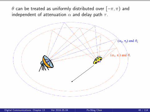
θ can be treated as uniformly distributed over [−π,π) andindependent of attenuation α and delay path τ .
Digital Communications: Chapter 13 Ver 2016.05.04 Po-Ning Chen 40 / 114
Channel model from IEEE 802.11 Handbook
A consistent channel model is required to allowcomparison among different WLAN systems.
The IEEE 802.11 Working Group adopted the followingchannel model as the baseline for predicting multipath formodulations used in IEEE 802.11a and IEEE 802.11b,which is ideal for software simulations.
The phase is uniformly distributed.
The magnitude is Rayleigh distributed with averagepower decaying exponentially.
Digital Communications: Chapter 13 Ver 2016.05.04 Po-Ning Chen 41 / 114
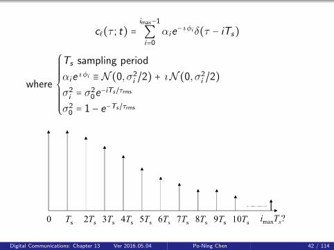
c`(τ ; t) =imax−1
∑i=0
αie− ı φi δ(τ − iTs)
where
⎧⎪⎪⎪⎪⎪⎪⎪⎨⎪⎪⎪⎪⎪⎪⎪⎩
Ts sampling period
αie ı φi ≡ N (0, σ2i /2) + ıN (0, σ2
i /2)σ2i = σ2
0e−iTs/τrms
σ20 = 1 − e−Ts/τrms
Digital Communications: Chapter 13 Ver 2016.05.04 Po-Ning Chen 42 / 114
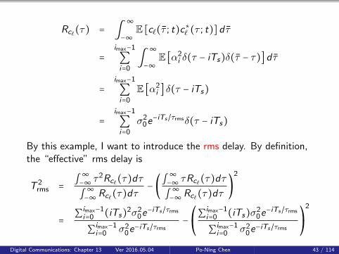
Rc`(τ) = ∫∞
−∞E [c`(τ ; t)c∗` (τ ; t)]d τ
=imax−1
∑i=0∫
∞
−∞E [α2
i δ(τ − iTs)δ(τ − τ)]d τ
=imax−1
∑i=0
E [α2i ] δ(τ − iTs)
=imax−1
∑i=0
σ20e
−iTs/τrmsδ(τ − iTs)
By this example, I want to introduce the rms delay. By definition,the “effective” rms delay is
T 2rms = ∫
∞−∞ τ
2Rc`(τ)dτ∫∞−∞ Rc`(τ)dτ
− (∫∞−∞ τRc`(τ)dτ∫∞−∞ Rc`(τ)dτ
)2
= ∑imax−1i=0 (iTs)2σ2
0e−iTs/τrms
∑imax−1i=0 σ2
0e−iTs/τrms
−⎛⎝∑imax−1
i=0 (iTs)σ20e
−iTs/τrms
∑imax−1i=0 σ2
0e−iTs/τrms
⎞⎠
2
Digital Communications: Chapter 13 Ver 2016.05.04 Po-Ning Chen 43 / 114
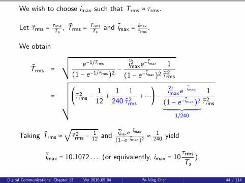
We wish to choose imax such that Trms ≈ τrms.
Let τrms = τrmsTs
, Trms = TrmsTs
and imax = imaxτrms
.
We obtain
Trms =
¿ÁÁÀ e−1/τrms
(1 − e−1/τrms)2− i2maxe
−imax
(1 − e−imax)2
1
τ2rms
=
¿ÁÁÁÁÁÁÀ
(τ2rms −
1
12+ 1
240
1
τ2rms
+⋯) − i2maxe−imax
(1 − e−imax)2
´¹¹¹¹¹¹¹¹¹¹¹¹¹¹¹¹¹¹¹¹¹¹¹¹¹¹¹¹¸¹¹¹¹¹¹¹¹¹¹¹¹¹¹¹¹¹¹¹¹¹¹¹¹¹¹¹¹¹¶1/240
1
τ2rms
Taking Trms ≈√τ2
rms − 112 and
i2maxe−imax
(1−e−imax)2≈ 1
240 yield
imax = 10.1072 . . . (or equivalently, imax = 10τrms
Ts).
Digital Communications: Chapter 13 Ver 2016.05.04 Po-Ning Chen 44 / 114
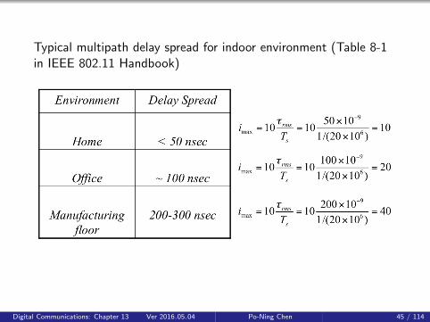
Typical multipath delay spread for indoor environment (Table 8-1in IEEE 802.11 Handbook)
Digital Communications: Chapter 13 Ver 2016.05.04 Po-Ning Chen 45 / 114
13.1-2 Statistical models for fadingchannels
Digital Communications: Chapter 13 Ver 2016.05.04 Po-Ning Chen 46 / 114

In addition to zero-mean Gaussian (Rayleigh), non-zero-meanGaussian (Rice) and Nakagami-m distributions, there are othermodels for c`(τ ; t) have been proposed in the literature.
Example.
Channels with a direct path and a single multipathcomponent, such as airplane-to-ground communications
c`(τ ; t) = αδ(τ) + β(t)δ(τ − τ0(t))
where α controls the power in the direct path and isnamed specular component, and β(t) is modeled aszero-mean Gaussian.
Digital Communications: Chapter 13 Ver 2016.05.04 Po-Ning Chen 47 / 114
Example.
Microwave LOS radio channels used for long-distancevoice and video transmission by telephone companies inthe 6 GHz band (Rummler 1979)
c`(τ) = α [δ(τ) − βe ı2πf0τδ(τ − τ0)]
where⎧⎪⎪⎪⎪⎪⎪⎪⎨⎪⎪⎪⎪⎪⎪⎪⎩
α overall attenuation parameter
β shape parameter due to multipath components
τ0 time delay
f0 frequency of the fade minimum, i.e., f0 = arg minf ∈R ∣C`(f )∣
Digital Communications: Chapter 13 Ver 2016.05.04 Po-Ning Chen 48 / 114
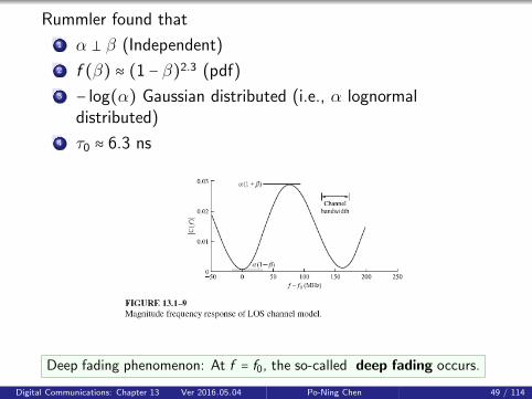
Rummler found that
1 α ⊥ β (Independent)
2 f (β) ≈ (1 − β)2.3 (pdf)
3 − log(α) Gaussian distributed (i.e., α lognormaldistributed)
4 τ0 ≈ 6.3 ns
Deep fading phenomenon: At f = f0, the so-called deep fading occurs.
Digital Communications: Chapter 13 Ver 2016.05.04 Po-Ning Chen 49 / 114

13.2 The effect of signalcharacteristics on the choice of a
channel model
Digital Communications: Chapter 13 Ver 2016.05.04 Po-Ning Chen 50 / 114
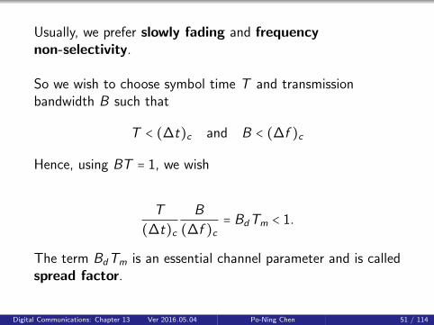
Usually, we prefer slowly fading and frequencynon-selectivity.
So we wish to choose symbol time T and transmissionbandwidth B such that
T < (∆t)c and B < (∆f )c
Hence, using BT = 1, we wish
T
(∆t)cB
(∆f )c= BdTm < 1.
The term BdTm is an essential channel parameter and is calledspread factor.
Digital Communications: Chapter 13 Ver 2016.05.04 Po-Ning Chen 51 / 114
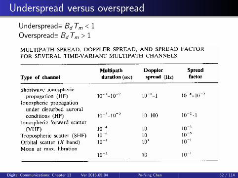
Underspread versus overspread
Underspread≡ BdTm < 1Overspread≡ BdTm > 1
Digital Communications: Chapter 13 Ver 2016.05.04 Po-Ning Chen 52 / 114
13.3 Frequency-nonslective, slowlyfading channel
Digital Communications: Chapter 13 Ver 2016.05.04 Po-Ning Chen 53 / 114
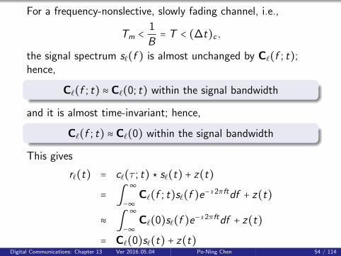
For a frequency-nonslective, slowly fading channel, i.e.,
Tm < 1
B= T < (∆t)c ,
the signal spectrum s`(f ) is almost unchanged by C`(f ; t);hence,
C`(f ; t) ≈ C`(0; t) within the signal bandwidth
and it is almost time-invariant; hence,
C`(f ; t) ≈ C`(0) within the signal bandwidth
This gives
r`(t) = c`(τ ; t) ⋆ s`(t) + z(t)
= ∫∞
−∞C`(f ; t)s`(f )e− ı2πftdf + z(t)
≈ ∫∞
−∞C`(0)s`(f )e− ı2πftdf + z(t)
= C`(0)s`(t) + z(t)Digital Communications: Chapter 13 Ver 2016.05.04 Po-Ning Chen 54 / 114
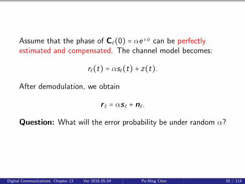
Assume that the phase of C`(0) = αe ı φ can be perfectlyestimated and compensated. The channel model becomes:
r`(t) = αs`(t) + z(t).
After demodulation, we obtain
r ` = αs` + n`.
Question: What will the error probability be under random α?
Digital Communications: Chapter 13 Ver 2016.05.04 Po-Ning Chen 55 / 114
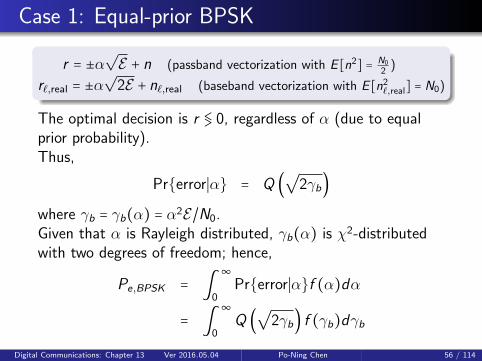
Case 1: Equal-prior BPSK
r = ±α√E + n (passband vectorization with E [n2] = N0
2)
r`,real = ±α√
2E + n`,real (baseband vectorization with E [n2`,real] = N0)
The optimal decision is r ≶ 0, regardless of α (due to equalprior probability).Thus,
Pr{error∣α} = Q (√
2γb)
where γb = γb(α) = α2E/N0.Given that α is Rayleigh distributed, γb(α) is χ2-distributedwith two degrees of freedom; hence,
Pe,BPSK = ∫∞
0Pr{error∣α}f (α)dα
= ∫∞
0Q (
√2γb) f (γb)dγb
Digital Communications: Chapter 13 Ver 2016.05.04 Po-Ning Chen 56 / 114
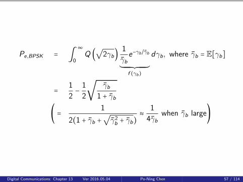
Pe,BPSK = ∫∞
0Q (
√2γb)
1
γbe−γb/γb
´¹¹¹¹¹¹¹¹¹¹¹¹¹¹¹¸¹¹¹¹¹¹¹¹¹¹¹¹¹¹¹¶f (γb)
dγb, where γb = E[γb]
= 1
2− 1
2
√γb
1 + γb
( = 1
2(1 + γb +√γ2b + γb)
≈ 1
4γbwhen γb large)
Digital Communications: Chapter 13 Ver 2016.05.04 Po-Ning Chen 57 / 114

Case 2: Equal-prior BFSK
Similarly, for BFSK,
r = {[α√E
0] or [ 0
α√E]} + n
The optimal decision is r1 ≶ r2, regardless of α.
Pe,BFSK = ∫∞
0Pr{error∣α}f (α)dα
= ∫∞
0Q (√γb) f (γb)dγb
= 1
2− 1
2
√γb
2 + γb
( = 1
2 + γb +√γ2b + 2γb
≈ 1
2γbwhen γb large)
Digital Communications: Chapter 13 Ver 2016.05.04 Po-Ning Chen 58 / 114
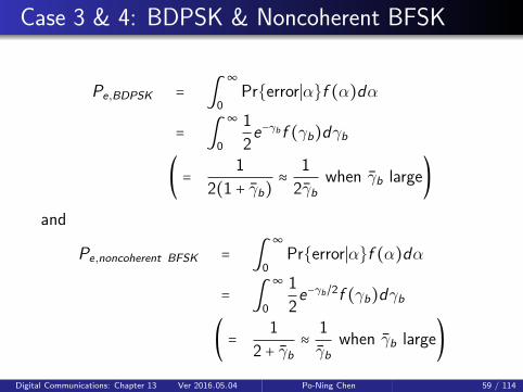
Case 3 & 4: BDPSK & Noncoherent BFSK
Pe,BDPSK = ∫∞
0Pr{error∣α}f (α)dα
= ∫∞
0
1
2e−γb f (γb)dγb
( = 1
2(1 + γb)≈ 1
2γbwhen γb large)
and
Pe,noncoherent BFSK = ∫∞
0Pr{error∣α}f (α)dα
= ∫∞
0
1
2e−γb/2f (γb)dγb
( = 1
2 + γb≈ 1
γbwhen γb large)
Digital Communications: Chapter 13 Ver 2016.05.04 Po-Ning Chen 59 / 114

Pe under AWGN Pe under Approx Pe underRayleigh fading Rayleigh fading
BPSK Q(√
2γb) 12 (1 −
√γb
1+γb )1
4γb
BFSK Q(√γb) 12 (1 −
√γb
2+γb )1
2γb
BDPSK 12e
−γb 12(1+γb)
12γb
NoncohrentBFSK
12e
−γb/2 12+γb
1γb
Digital Communications: Chapter 13 Ver 2016.05.04 Po-Ning Chen 60 / 114

● BPSK is 3dB better thanBDPSK/BFSK; 6dBbetter than noncoherentBFSK.● Pe decreases inverselyproportional with SNRunder fading.
● Pe decreases exponentiallywith SNRwhen no fading.
Digital Communications: Chapter 13 Ver 2016.05.04 Po-Ning Chen 61 / 114
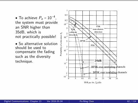
● To achieve Pe = 10−4,the system must providean SNR higher than35dB, which isnot practically possible!
● So alternative solutionshould be used tocompensate the fadingsuch as the diversitytechnique.
Digital Communications: Chapter 13 Ver 2016.05.04 Po-Ning Chen 62 / 114
Nakagami fading
If α ≡ Nakagami-m fading,
Turin et al. (1972) and Suzuki (1977) have shown that theNakagami-m distribution is the best-fit for urban radio multipathchannels.
Ô⇒ f (γb) = mm
Γ(m)γmbγm−1b e−mγb/γb , where γb = E [α2]Eb/N0.
m < 1: Worse than Rayleigh fading in performance
m = 1: Rayleigh fading
m > 1: Better than Rayleigh fading in performance
Digital Communications: Chapter 13 Ver 2016.05.04 Po-Ning Chen 63 / 114
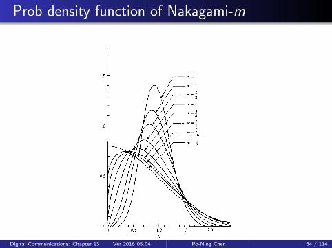
Prob density function of Nakagami-m
Digital Communications: Chapter 13 Ver 2016.05.04 Po-Ning Chen 64 / 114
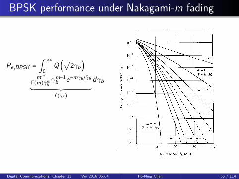
BPSK performance under Nakagami-m fading
Pe,BPSK = ∫∞
0Q (
√2γb)
mm
Γ(m)γmbγm−1b e−mγb/γb
´¹¹¹¹¹¹¹¹¹¹¹¹¹¹¹¹¹¹¹¹¹¹¹¹¹¹¹¹¹¹¹¹¹¹¹¹¹¹¹¹¹¹¹¹¹¹¹¹¹¹¹¹¹¹¹¹¹¸¹¹¹¹¹¹¹¹¹¹¹¹¹¹¹¹¹¹¹¹¹¹¹¹¹¹¹¹¹¹¹¹¹¹¹¹¹¹¹¹¹¹¹¹¹¹¹¹¹¹¹¹¹¹¹¹¹¹¶f (γb)
dγb
Digital Communications: Chapter 13 Ver 2016.05.04 Po-Ning Chen 65 / 114

In some channel, the system performance may degrade evenworse, such as Rummler’s model in slide 13-48, where deepfading occurs at some frequency.
∣C`(f )∣
The lowest is equal to α(1 − β), which is itself a random variable (which
makes the performance worse as we have seen from Rayleigh example
study) even if f0 is fixed!
Digital Communications: Chapter 13 Ver 2016.05.04 Po-Ning Chen 66 / 114

13.4 Diversity techniques for fadingmultipath channels
Digital Communications: Chapter 13 Ver 2016.05.04 Po-Ning Chen 67 / 114
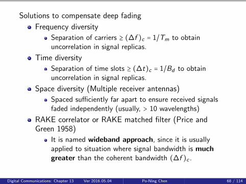
Solutions to compensate deep fading
Frequency diversity
Separation of carriers ≥ (∆f )c = 1/Tm to obtainuncorrelation in signal replicas.
Time diversity
Separation of time slots ≥ (∆t)c = 1/Bd to obtainuncorrelation in signal replicas.
Space diversity (Multiple receiver antennas)
Spaced sufficiently far apart to ensure received signalsfaded independently (usually, > 10 wavelengths)
RAKE correlator or RAKE matched filter (Price andGreen 1958)
It is named wideband approach, since it is usuallyapplied to situation where signal bandwidth is muchgreater than the coherent bandwidth (∆f )c .
Digital Communications: Chapter 13 Ver 2016.05.04 Po-Ning Chen 68 / 114

It is clear for the first three diversities, we will have L identicalreplicas at the Rx (which are uncorrelated).
The idea is that as long as not all of them are deep-faded, thedemodulation is “ok.”
For the last one (i.e., RAKE), where B ≫ (∆f )c , which resultsin a frequency selective channel, we have
L = B
(∆f )c.
Detail will be given later.
Digital Communications: Chapter 13 Ver 2016.05.04 Po-Ning Chen 69 / 114

13.4-1 Binary signals
Digital Communications: Chapter 13 Ver 2016.05.04 Po-Ning Chen 70 / 114

Assumption
1 L identical and independent channels.
2 Each channel is frequency-nonselective and slowlyfading with Rayleigh-distributed envelope.
3 Zero-mean additive white Gaussian background noise.
4 Assume the phase-shift can be perfectly compensated.
5 Assume the attenuation {αk}Lk=1 can be perfectlyestimated at Rx.
Hence,rk = αks + nk k = 1,2, . . . ,L
How to combine these L outputs when making decision?Maximal ratio combiner (Brennan 1959)
r =L
∑k=1
αkrk =L
∑k=1
α2ks +
L
∑k=1
αknk .
Digital Communications: Chapter 13 Ver 2016.05.04 Po-Ning Chen 71 / 114

Idea behind maximal ratio combiner
Trust more on the strong signals and trust less on theweak signal.
Advantage of maximal ratio combiner
Theoretically tractable; so we can predict how “good” thesystem can achieve without performing simulations.
Digital Communications: Chapter 13 Ver 2016.05.04 Po-Ning Chen 72 / 114
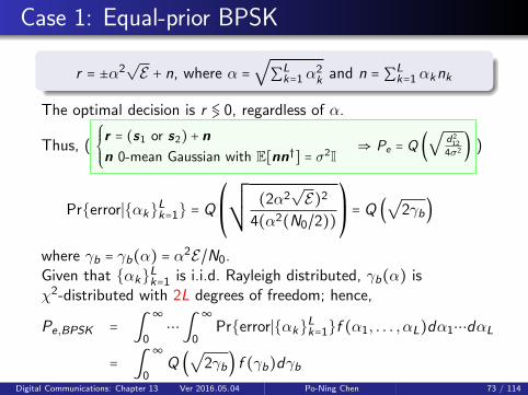
Case 1: Equal-prior BPSK
r = ±α2√E + n, where α =
√∑L
k=1 α2k and n = ∑L
k=1 αknk
The optimal decision is r ≶ 0, regardless of α.
Thus, (⎧⎪⎪⎨⎪⎪⎩
r = (s1 or s2) + nn 0-mean Gaussian with E[nn†] = σ2I
⇒ Pe = Q (√
d212
4σ2 ) )
Pr{error∣{αk}Lk=1} = Q⎛⎜⎝
¿ÁÁÀ (2α2
√E)2
4(α2(N0/2))
⎞⎟⎠= Q (
√2γb)
where γb = γb(α) = α2E/N0.Given that {αk}Lk=1 is i.i.d. Rayleigh distributed, γb(α) isχ2-distributed with 2L degrees of freedom; hence,
Pe,BPSK = ∫∞
0⋯∫
∞
0Pr{error∣{αk}Lk=1}f (α1, . . . , αL)dα1⋯dαL
= ∫∞
0Q (
√2γb) f (γb)dγb
Digital Communications: Chapter 13 Ver 2016.05.04 Po-Ning Chen 73 / 114
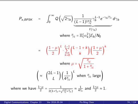
Pe,BPSK = ∫∞
0Q (
√2γb)
1
(L − 1)!γLcγL−1b e−γb/γc
´¹¹¹¹¹¹¹¹¹¹¹¹¹¹¹¹¹¹¹¹¹¹¹¹¹¹¹¹¹¹¹¹¹¹¹¹¹¹¹¹¹¹¹¹¹¹¹¹¹¹¹¹¹¹¹¹¹¹¹¹¹¹¹¹¸¹¹¹¹¹¹¹¹¹¹¹¹¹¹¹¹¹¹¹¹¹¹¹¹¹¹¹¹¹¹¹¹¹¹¹¹¹¹¹¹¹¹¹¹¹¹¹¹¹¹¹¹¹¹¹¹¹¹¹¹¹¹¹¹¶f (γb)
dγb
where γc = E[α2k]Eb/N0
= (1 − µ2
)L
⋅L−1
∑k=0
(L − 1 + k
k)(1 + µ
2)k
where µ =√
γc1 + γc
( ≈ (2L − 1
L)( 1
4γc)L
when γc large)
where we have 1−µ2 = 1
2(1+γc+√γ2c+γc)
≈ 14γc
and 1+µ2 ≈ 1.
Digital Communications: Chapter 13 Ver 2016.05.04 Po-Ning Chen 74 / 114
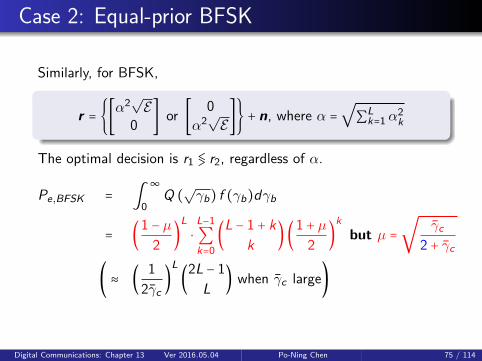
Case 2: Equal-prior BFSK
Similarly, for BFSK,
r = {[α2√E
0] or [ 0
α2√E]} + n, where α =
√∑L
k=1 α2k
The optimal decision is r1 ≶ r2, regardless of α.
Pe,BFSK = ∫∞
0Q (√γb) f (γb)dγb
= (1 − µ2
)L
⋅L−1
∑k=0
(L − 1 + k
k)(1 + µ
2)k
but µ =√
γc2 + γc
( ≈ ( 1
2γc)L
(2L − 1
L) when γc large)
Digital Communications: Chapter 13 Ver 2016.05.04 Po-Ning Chen 75 / 114

Case 3: BDPSK
From Slide 4-184 with t being the time index,
m = arg max1≤m≤2
Re{(r (t−1)` )
∗r (t)` e− ı θm}
= arg max(Re{(r (t−1)` )
∗r (t)` }
´¹¹¹¹¹¹¹¹¹¹¹¹¹¹¹¹¹¹¹¹¹¹¹¹¹¹¹¹¹¹¹¹¹¹¹¹¹¹¹¹¹¹¹¹¹¹¹¹¹¹¹¹¹¸¹¹¹¹¹¹¹¹¹¹¹¹¹¹¹¹¹¹¹¹¹¹¹¹¹¹¹¹¹¹¹¹¹¹¹¹¹¹¹¹¹¹¹¹¹¹¹¹¹¹¹¹¹¶m=1
,−Re{(r (t−1)` )
∗r (t)` }
´¹¹¹¹¹¹¹¹¹¹¹¹¹¹¹¹¹¹¹¹¹¹¹¹¹¹¹¹¹¹¹¹¹¹¹¹¹¹¹¹¹¹¹¹¹¹¹¹¹¹¹¹¹¹¹¹¹¹¸¹¹¹¹¹¹¹¹¹¹¹¹¹¹¹¹¹¹¹¹¹¹¹¹¹¹¹¹¹¹¹¹¹¹¹¹¹¹¹¹¹¹¹¹¹¹¹¹¹¹¹¹¹¹¹¹¹¹¶m=2
)
Now with L previous receptions and L current receptions,
m = arg max(U`m=1
, −U`±m=2
)
where U` =L
∑k=1
Re{(r (t−1)k,` )
∗r(t)k,` }
=L
∑k=1
Re{(αks(t−1)` + n
(t−1)k,` )
∗(αks
(t)` + n
(t)k,`)}
which closely resembles maximal ratio combining.Digital Communications: Chapter 13 Ver 2016.05.04 Po-Ning Chen 76 / 114

With some lengthy derivation, we obtain
Pe,BDPSK = (1 − µ2
)L
⋅L−1
∑k=0
(L − 1 + k
k)(1 + µ
2)k
but µ = γc1 + γc
≈ ( 1
2γc)L
(2L − 1
L) when γc large.
Digital Communications: Chapter 13 Ver 2016.05.04 Po-Ning Chen 77 / 114

Case 4: Noncoherent FSK
Recall from Slide 4-165:
The noncoherent ML computes
m = arg max1≤m≤M
∣r †`sm,`∣
From Slide 4-174,
s1,` = (√
2Es 0 ⋯ 0 )s2,` = ( 0
√2Es ⋯ 0 )
⋮ = ( ⋮ ⋮ ⋱ ⋮ )sM,` = ( 0 0 ⋯
√2Es )
Hence,
m = arg max1≤m≤M
∣rm,`∣ = arg max1≤m≤M
∣rm,`∣2.
Digital Communications: Chapter 13 Ver 2016.05.04 Po-Ning Chen 78 / 114
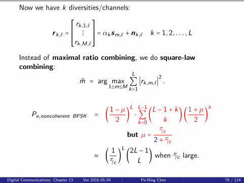
Now we have k diversities/channels:
rk,` =⎡⎢⎢⎢⎢⎢⎣
rk,1,`⋮
rk,M,`
⎤⎥⎥⎥⎥⎥⎦= αksm,` + nk,` k = 1,2, . . . ,L
Instead of maximal ratio combining, we do square-lawcombining:
m = arg max1≤m≤M
L
∑k=1
∣rk,m,`∣2.
Pe,noncoherent BFSK = (1 − µ2
)L
⋅L−1
∑k=0
(L − 1 + k
k)(1 + µ
2)k
but µ = γc2 + γc
≈ ( 1
γc)L
(2L − 1
L) when γc large.
Digital Communications: Chapter 13 Ver 2016.05.04 Po-Ning Chen 79 / 114
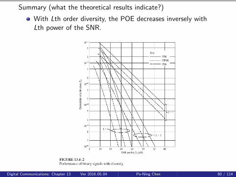
Summary (what the theoretical results indicate?)
With Lth order diversity, the POE decreases inversely withLth power of the SNR.
Digital Communications: Chapter 13 Ver 2016.05.04 Po-Ning Chen 80 / 114
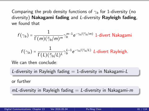
Comparing the prob density functions of γb for 1-diversity (nodiversity) Nakagami fading and L-diversity Rayleigh fading,we found that
f (γb) =1
Γ(m)(γb/m)mγm−1b e−γb/(γb/m) 1-divert Nakagami
f (γb) =1
Γ(L)(γb/L)LγL−1b e−γb/(γb/L) L-divert Rayleigh.
We can then conclude:
L-diversity in Rayleigh fading = 1-diversity in Nakagami-L
or further
mL-diversity in Rayleigh fading = L-diversity in Nakagami-m
Digital Communications: Chapter 13 Ver 2016.05.04 Po-Ning Chen 81 / 114

13.4-2 Multiphase signals
Digital Communications: Chapter 13 Ver 2016.05.04 Po-Ning Chen 82 / 114
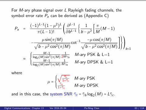
For M-ary phase signal over L Rayleigh fading channels, thesymbol error rate Pe can be derived as (Appendix C)
Pe = (−1)L−1(1 − µ2)L
π(L − 1)!( ∂L−1
∂bL−1{ 1
b − µ2[ πM
(M − 1)
− µ sin(π/M)√b − µ2 cos2(π/M)
cot−1 −µ cos(π/M)√b − µ2 cos2(π/M)
⎤⎥⎥⎥⎦
⎫⎪⎪⎬⎪⎪⎭
⎞⎠b=1
≈⎧⎪⎪⎨⎪⎪⎩
M−1log2(M) sin2(π/M)
12Mγb
M-ary PSK & L=1
M−1log2(M) sin2(π/M)
1Mγb
M-ary DPSK & L=1
where
µ =⎧⎪⎪⎨⎪⎪⎩
√γc
1+γc M-ary PSKγc
1+γc M-ary DPSK
and in this case, the system SNR γt = γb log2(M) = Lγc .
Digital Communications: Chapter 13 Ver 2016.05.04 Po-Ning Chen 83 / 114
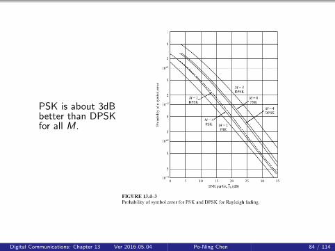
PSK is about 3dBbetter than DPSKfor all M.
Digital Communications: Chapter 13 Ver 2016.05.04 Po-Ning Chen 84 / 114
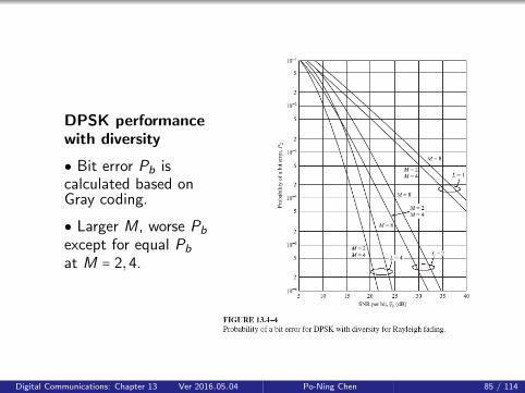
DPSK performancewith diversity
● Bit error Pb iscalculated based onGray coding.
● Larger M, worse Pb
except for equal Pb
at M = 2,4.
Digital Communications: Chapter 13 Ver 2016.05.04 Po-Ning Chen 85 / 114
13.4-3 M-ary orthogonal signals
Digital Communications: Chapter 13 Ver 2016.05.04 Po-Ning Chen 86 / 114
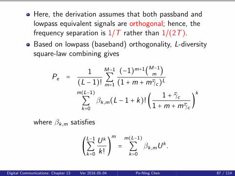
Here, the derivation assumes that both passband andlowpass equivalent signals are orthogonal; hence, thefrequency separation is 1/T rather than 1/(2T ).
Based on lowpass (baseband) orthogonality, L-diversitysquare-law combining gives
Pe = 1
(L − 1)!
M−1
∑m=1
(−1)m+1(M−1m
)(1 +m +mγc)L
m(L−1)
∑k=0
βk,m(L − 1 + k)!( 1 + γc1 +m +mγc
)k
where βk,m satisfies
(L−1
∑k=0
Uk
k!)m
=m(L−1)
∑k=0
βk,mUk .
Digital Communications: Chapter 13 Ver 2016.05.04 Po-Ning Chen 87 / 114
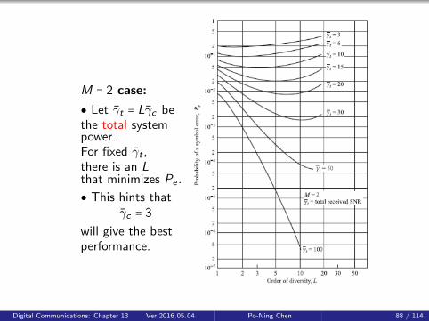
M = 2 case:
● Let γt = Lγc bethe total systempower.For fixed γt ,there is an Lthat minimizes Pe .
● This hints thatγc = 3
will give the bestperformance.
Digital Communications: Chapter 13 Ver 2016.05.04 Po-Ning Chen 88 / 114
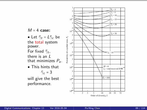
M = 4 case:
● Let γt = Lγc bethe total systempower.For fixed γt ,there is an Lthat minimizes Pe .
● This hints thatγc = 3
will give the bestperformance.
Digital Communications: Chapter 13 Ver 2016.05.04 Po-Ning Chen 89 / 114

Discussions:● Larger M, better performancebut larger bandwidth.
● Larger L, better performance.
● An increase in Lis more efficientin performance gainthan an increasein M.
Digital Communications: Chapter 13 Ver 2016.05.04 Po-Ning Chen 90 / 114

13.5 Digital signaling over afrequency-selective, slowly fading
channel
Digital Communications: Chapter 13 Ver 2016.05.04 Po-Ning Chen 91 / 114
13.5.1 A tapped-delay-line channelmodel
Digital Communications: Chapter 13 Ver 2016.05.04 Po-Ning Chen 92 / 114
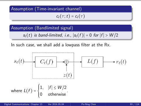
Assumption (Time-invariant channel)
c`(τ ; t) = c`(τ)
Assumption (Bandlimited signal)
s`(t) is band-limited, i.e., ∣s`(f )∣ = 0 for ∣f ∣ >W /2
In such case, we shall add a lowpass filter at the Rx.
where L(f ) =⎧⎪⎪⎨⎪⎪⎩
1, ∣f ∣ ≤W /2
0 otherwise.
Digital Communications: Chapter 13 Ver 2016.05.04 Po-Ning Chen 93 / 114

r`(t) = ∫∞
−∞s`(f )C`(f )e ı2πftdf + zW (t)
Digital Communications: Chapter 13 Ver 2016.05.04 Po-Ning Chen 94 / 114

For a bandlimited C`(f ), sampling theorem gives:
⎧⎪⎪⎪⎪⎪⎪⎪⎪⎪⎪⎪⎪⎪⎪⎪⎪⎨⎪⎪⎪⎪⎪⎪⎪⎪⎪⎪⎪⎪⎪⎪⎪⎪⎩
c`(t) =∞∑
n=−∞c` (
n
W) sinc(W (t − n
W))
C`(f ) = ∫∞
−∞c`(t)e− ı2πftdt
=⎧⎪⎪⎪⎨⎪⎪⎪⎩
1
W
∞∑
n=−∞c` (
n
W) e− ı2πfn/W , ∣f ∣ ≤W /2
0, otherwise
Digital Communications: Chapter 13 Ver 2016.05.04 Po-Ning Chen 95 / 114
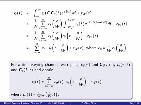
r`(t) = ∫∞
−∞s`(f )C`(f )e ı2πftdf + zW (t)
= 1
W
∞∑
n=−∞c` (
n
W)∫
W /2
−W /2s`(f )e ı2πf (t−n/W )df + zW (t)
= 1
W
∞∑
n=−∞c` (
n
W) s` (t −
n
W) + zW (t)
=∞∑
n=−∞cn ⋅ s` (t −
n
W) + zW (t), where cn =
1
Wc` (
n
W)
For a time-varying channel, we replace c`(τ) and C`(f ) by c`(τ ; t)and C`(f ; t) and obtain
r`(t) =∞∑
n=−∞cn(t) ⋅ s` (t −
n
W) + zW (t)
where cn(t) = 1W c` ( n
W ; t) .
Digital Communications: Chapter 13 Ver 2016.05.04 Po-Ning Chen 96 / 114
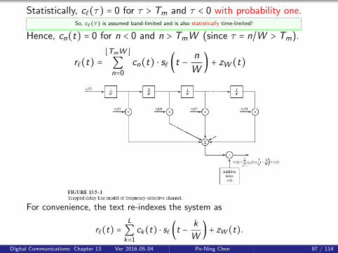
Statistically, c`(τ) = 0 for τ > Tm and τ < 0 with probability one.So, c`(τ) is assumed band-limited and is also statistically time-limited!
Hence, cn(t) = 0 for n < 0 and n > TmW (since τ = n/W > Tm).
r`(t) =⌊TmW ⌋∑n=0
cn(t) ⋅ s` (t −n
W) + zW (t)
For convenience, the text re-indexes the system as
r`(t) =L
∑k=1
ck(t) ⋅ s` (t −k
W) + zW (t).
Digital Communications: Chapter 13 Ver 2016.05.04 Po-Ning Chen 97 / 114
13.5-2 The RAKE demodulator
Digital Communications: Chapter 13 Ver 2016.05.04 Po-Ning Chen 98 / 114

Assumption (Gaussian and US (uncorrelated scattering))
{ck(t)}Lk=1 complex i.i.d. Gaussian and can be perfectly estimatedby Rx.
So the Rx can regard the “transmitted signal” as one of
⎧⎪⎪⎪⎨⎪⎪⎪⎩
v1,`(t) = ∑Lk=1 ck(t) ⋅ s1,` (t − k
W)
⋮vM,`(t) = ∑L
k=1 ck(t) ⋅ sM,` (t − kW
)
So Slide 4-166 said:
Coherent MAP detection
m = arg max1≤m≤M
Re [r †`vm,`] = arg max
1≤m≤MRe [∫
T
0r`(t)v∗m,`(t)dt]
= arg max1≤m≤M
Re [L
∑k=1∫
T
0r`(t)c∗k (t)s
∗m,` (t −
k
W)dt]
´¹¹¹¹¹¹¹¹¹¹¹¹¹¹¹¹¹¹¹¹¹¹¹¹¹¹¹¹¹¹¹¹¹¹¹¹¹¹¹¹¹¹¹¹¹¹¹¹¹¹¹¹¹¹¹¹¹¹¹¹¹¹¹¹¹¹¹¹¹¹¹¹¹¹¹¹¹¹¹¹¹¹¹¹¹¹¹¹¹¹¹¹¹¹¹¹¹¹¹¹¹¹¹¹¹¹¹¹¹¹¹¹¹¹¹¹¹¹¹¹¹¹¹¹¹¹¹¹¹¹¹¸¹¹¹¹¹¹¹¹¹¹¹¹¹¹¹¹¹¹¹¹¹¹¹¹¹¹¹¹¹¹¹¹¹¹¹¹¹¹¹¹¹¹¹¹¹¹¹¹¹¹¹¹¹¹¹¹¹¹¹¹¹¹¹¹¹¹¹¹¹¹¹¹¹¹¹¹¹¹¹¹¹¹¹¹¹¹¹¹¹¹¹¹¹¹¹¹¹¹¹¹¹¹¹¹¹¹¹¹¹¹¹¹¹¹¹¹¹¹¹¹¹¹¹¹¹¹¹¹¹¹¹¹¶Um,`
Digital Communications: Chapter 13 Ver 2016.05.04 Po-Ning Chen 99 / 114
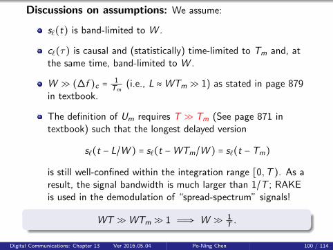
Discussions on assumptions: We assume:
s`(t) is band-limited to W .
c`(τ) is causal and (statistically) time-limited to Tm and, atthe same time, band-limited to W .
W ≫ (∆f )c = 1Tm
(i.e., L ≈WTm ≫ 1) as stated in page 879in textbook.
The definition of Um requires T ≫ Tm (See page 871 intextbook) such that the longest delayed version
s`(t − L/W ) = s`(t −WTm/W ) = s`(t −Tm)
is still well-confined within the integration range [0,T ). As aresult, the signal bandwidth is much larger than 1/T ; RAKEis used in the demodulation of “spread-spectrum” signals!
WT ≫WTm ≫ 1 Ô⇒ W ≫ 1T .
Digital Communications: Chapter 13 Ver 2016.05.04 Po-Ning Chen 100 / 114
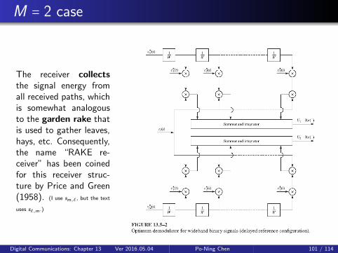
M = 2 case
The receiver collectsthe signal energy fromall received paths, whichis somewhat analogousto the garden rake thatis used to gather leaves,hays, etc. Consequently,the name “RAKE re-ceiver” has been coinedfor this receiver struc-ture by Price and Green(1958). (I use sm,`, but the text
uses s`,m .)
Digital Communications: Chapter 13 Ver 2016.05.04 Po-Ning Chen 101 / 114
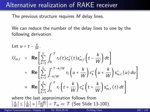
Alternative realization of RAKE receiver
The previous structure requires M delay lines.
We can reduce the number of the delay lines to one by thefollowing derivation.
Let u = t − kW .
Um,` = Re [L
∑k=1∫
T
0r`(t)c∗k (t)s∗m,` (t −
k
W)dt]
= Re [L
∑k=1∫
T−k/W
−k/Wr` (u +
k
W) c∗k (u + k
W) s∗m,` (u)du]
≈ Re [L
∑k=1∫
T
0r` (t +
k
W) c∗k (t + k
W) s∗m,` (t)dt]
where the last approximation follows from∣ kW
∣ ≤ ∣ LW
∣ ≈ ∣TmWW
∣ = Tm ≪ T (See Slide 13-100).Digital Communications: Chapter 13 Ver 2016.05.04 Po-Ning Chen 102 / 114
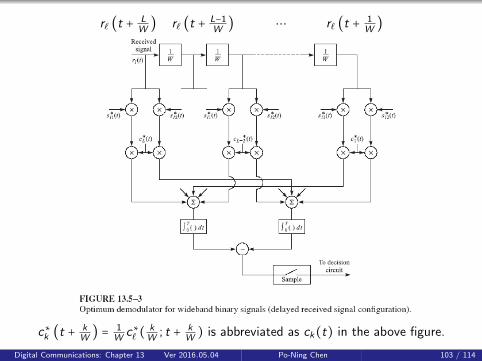
r` (t + LW
) r` (t + L−1W
) ⋯ r` (t + 1W
)
c∗k (t + kW
) = 1Wc∗` (
kW
; t + kW
) is abbreviated as ck(t) in the above figure.
Digital Communications: Chapter 13 Ver 2016.05.04 Po-Ning Chen 103 / 114
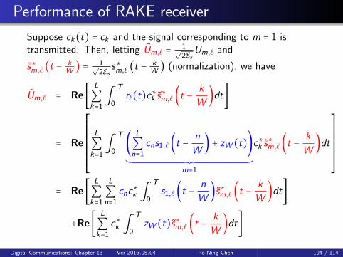
Performance of RAKE receiver
Suppose ck(t) = ck and the signal corresponding to m = 1 istransmitted. Then, letting Um,` = 1√
2EsUm,` and
s∗m,` (t −kW
) = 1√2Es
s∗m,` (t −kW
) (normalization), we have
Um,` = Re [L
∑k=1∫
T
0r`(t)c∗k s
∗m,` (t −
k
W)dt]
= Re
⎡⎢⎢⎢⎢⎢⎢⎢⎢⎢⎣
L
∑k=1∫
T
0(
L
∑n=1
cns1,` (t −n
W) + zW (t))
´¹¹¹¹¹¹¹¹¹¹¹¹¹¹¹¹¹¹¹¹¹¹¹¹¹¹¹¹¹¹¹¹¹¹¹¹¹¹¹¹¹¹¹¹¹¹¹¹¹¹¹¹¹¹¹¹¹¹¹¹¹¹¹¹¹¹¹¹¹¹¹¹¹¹¹¹¹¹¹¹¹¹¹¹¹¹¹¹¹¹¹¹¸¹¹¹¹¹¹¹¹¹¹¹¹¹¹¹¹¹¹¹¹¹¹¹¹¹¹¹¹¹¹¹¹¹¹¹¹¹¹¹¹¹¹¹¹¹¹¹¹¹¹¹¹¹¹¹¹¹¹¹¹¹¹¹¹¹¹¹¹¹¹¹¹¹¹¹¹¹¹¹¹¹¹¹¹¹¹¹¹¹¹¹¹¶m=1
c∗k s∗m,` (t −
k
W)dt
⎤⎥⎥⎥⎥⎥⎥⎥⎥⎥⎦
= Re [L
∑k=1
L
∑n=1
cnc∗k ∫
T
0s1,` (t −
n
W)s∗m,` (t −
k
W)dt]
+Re [L
∑k=1
c∗k ∫T
0zW (t)s∗m,` (t −
k
W)dt]
Digital Communications: Chapter 13 Ver 2016.05.04 Po-Ning Chen 104 / 114
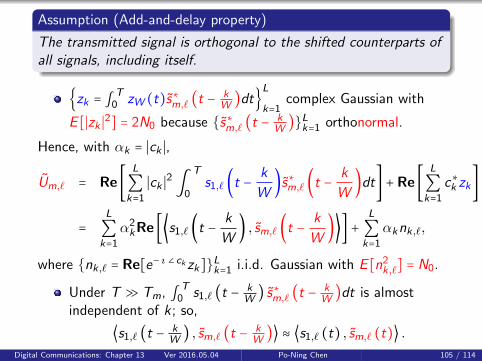
Assumption (Add-and-delay property)
The transmitted signal is orthogonal to the shifted counterparts ofall signals, including itself.
{zk = ∫T
0 zW (t)s∗m,` (t −kW
)dt}L
k=1complex Gaussian with
E [∣zk ∣2] = 2N0 because {s∗m,` (t −kW
)}Lk=1 orthonormal.
Hence, with αk = ∣ck ∣,
Um,` = Re [L
∑k=1
∣ck ∣2∫T
0s1,` (t −
k
W)s∗m,` (t −
k
W)dt] +Re [
L
∑k=1
c∗k zk]
=L
∑k=1
α2kRe [⟨s1,` (t −
k
W) , sm,` (t −
k
W)⟩] +
L
∑k=1
αknk,`,
where {nk,` = Re[e− ı∠ck zk]}Lk=1 i.i.d. Gaussian with E [n2k,`] = N0.
Under T ≫ Tm, ∫T
0 s1,` (t − kW
) s∗m,` (t −kW
)dt is almostindependent of k ; so,
⟨s1,` (t − kW
) , sm,` (t − kW
)⟩ ≈ ⟨s1,` (t) , sm,` (t)⟩ .Digital Communications: Chapter 13 Ver 2016.05.04 Po-Ning Chen 105 / 114
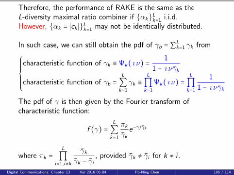
Therefore, the performance of RAKE is the same as theL-diversity maximal ratio combiner if {αk}Lk=1 i.i.d.However, {αk = ∣ck ∣}Lk=1 may not be identically distributed.
In such case, we can still obtain the pdf of γb = ∑Lk=1 γk from
⎧⎪⎪⎪⎪⎪⎨⎪⎪⎪⎪⎪⎩
characteristic function of γk ≡ Ψk( ı ν) =1
1 − ı νγkcharacteristic function of γb =
L
∑k=1
γk ≡L
∏k=1
Ψk( ı ν) =L
∏k=1
1
1 − ı νγkThe pdf of γ is then given by the Fourier transform ofcharacteristic function:
f (γ) =L
∑k=1
πkγk
e−γ/γk
where πk =L
∏i=1,i≠k
γkγk − γi
, provided γk ≠ γi for k ≠ i .
Digital Communications: Chapter 13 Ver 2016.05.04 Po-Ning Chen 106 / 114
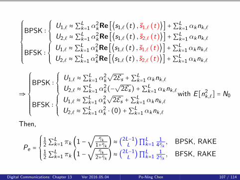
⎧⎪⎪⎪⎪⎪⎪⎪⎪⎨⎪⎪⎪⎪⎪⎪⎪⎪⎩
BPSK ∶⎧⎪⎪⎨⎪⎪⎩
U1,` ≈ ∑Lk=1 α
2kRe [⟨s1,` (t) , s1,` (t)⟩] +∑L
k=1 αknk,`
U2,` ≈ ∑Lk=1 α
2kRe [⟨s1,` (t) , s2,` (t)⟩] +∑L
k=1 αknk,`
BFSK ∶⎧⎪⎪⎨⎪⎪⎩
U1,` ≈ ∑Lk=1 α
2kRe [⟨s1,` (t) , s1,` (t)⟩] +∑L
k=1 αknk,`
U2,` ≈ ∑Lk=1 α
2kRe [⟨s1,` (t) , s2,` (t)⟩] +∑L
k=1 αknk,`
⇒
⎧⎪⎪⎪⎪⎪⎪⎪⎪⎨⎪⎪⎪⎪⎪⎪⎪⎪⎩
BPSK ∶⎧⎪⎪⎨⎪⎪⎩
U1,` ≈ ∑Lk=1 α
2k
√2Es +∑L
k=1 αknk,`
U2,` ≈ ∑Lk=1 α
2k(−
√2Es) +∑L
k=1 αknk,`
BFSK ∶⎧⎪⎪⎨⎪⎪⎩
U1,` ≈ ∑Lk=1 α
2k
√2Es +∑L
k=1 αknk,`
U2,` ≈ ∑Lk=1 α
2k ⋅ (0) +∑L
k=1 αknk,`
with E [n2k,`] = N0
Then,
Pe =⎧⎪⎪⎪⎨⎪⎪⎪⎩
12 ∑
Lk=1 πk (1 −
√γk
1+γk ) ≈ (2L−1L
)∏Lk=1
14γk, BPSK, RAKE
12 ∑
Lk=1 πk (1 −
√γk
2+γk ) ≈ (2L−1L
)∏Lk=1
12γk, BFSK, RAKE
Digital Communications: Chapter 13 Ver 2016.05.04 Po-Ning Chen 107 / 114

Estimation of ck
For orthogonal signaling, we can estimate cn via
∫T
0r` (t +
n
W)(s∗1,`(t) +⋯ + s∗M,`(t))dt
=L
∑k=1
ck ∫T
0sm,` (t +
n
W− k
W)(s∗1,`(t) +⋯ + s∗M,`(t))dt
+∫T
0z (t + n
W)(s∗1,`(t) +⋯ + s∗M,`(t))dt
=L
∑k=1
ck ∫T
0sm,` (t +
n
W− k
W) s∗m,`(t)dt
+∫T
0z (t + n
W)(s∗1,`(t) +⋯ + s∗M,`(t))dt (Orthogonality)
= cn ∫T
0∣sm,` (t) ∣2dt + noise term (Add-and-delay)
Digital Communications: Chapter 13 Ver 2016.05.04 Po-Ning Chen 108 / 114

M = 2 case
Bd = Doppler spread
Digital Communications: Chapter 13 Ver 2016.05.04 Po-Ning Chen 109 / 114
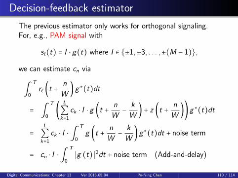
Decision-feedback estimator
The previous estimator only works for orthogonal signaling.For, e.g., PAM signal with
s`(t) = I ⋅ g(t) where I ∈ {±1,±3, . . . ,±(M − 1)},
we can estimate cn via
∫T
0r` (t +
n
W)g∗(t)dt
= ∫T
0(
L
∑k=1
ck ⋅ I ⋅ g (t + n
W− k
W) + z (t + n
W))g∗(t)dt
=L
∑k=1
ck ⋅ I ⋅ ∫T
0g (t + n
W− k
W)g∗(t)dt + noise term
= cn ⋅ I ⋅ ∫T
0∣g (t) ∣2dt + noise term (Add-and-delay)
Digital Communications: Chapter 13 Ver 2016.05.04 Po-Ning Chen 110 / 114
Final notes
Usually it requires (∆t)cT > 100 in order to have an accurate
estimate of {cn}Ln=1.
Note that for DPSK and FSK with square-law combiner, it isunnecessary to estimate {cn}Ln=1.
So, they have no further performance loss (due to aninaccurate estimate of {cn}Ln=1).
Digital Communications: Chapter 13 Ver 2016.05.04 Po-Ning Chen 111 / 114
What you learn from Chapter 13
Statistical model of (US-WSS) (linear) multipath fadingchannels:
c`(τ ; t) = c(τ ; t)e− ı2πfcτ and c(τ ; t) = ∣c`(τ ; t)∣Multipath intensity profile or delay power spectrum
Rc` (τ) = Rc` (τ ; ∆t = 0) .
Multipath delay spread Tm vs coherent bandwidth (∆f )cFrequency-selective vs frequency-nonselectiveSpaced-frequency, spaced-time correlation function
RC`(∆f ; ∆t) = E{C`(f +∆f ; t +∆t)C∗` (f ; t)}
Digital Communications: Chapter 13 Ver 2016.05.04 Po-Ning Chen 112 / 114

Doppler power spectrum
SC`(λ) = ∫∞
−∞RC`(∆f = 0; ∆t)e− ı2πλ(∆t)d(∆t)
Doppler spread Bd vs coherent time (∆t)cSlow fading versus fast fadingScattering function
S(τ ;λ) = F∆t {Rc`(τ ; ∆t)}
(Good to know) Jakes’ modelRayleigh, Rice and Nakagami-m, Rummler’s 3-pathmodelDeep fading phenomenonBdTm spread factor: Underspread vs overspread
Digital Communications: Chapter 13 Ver 2016.05.04 Po-Ning Chen 113 / 114

Analysis of error rate under frequency-nonselective, slowlyRayleigh- and Nakagami-m-distributed fading channels(≡diversity under Rayleigh) with M = 2
(Good to know) Analysis of the error rate ⋯ with M > 2.
Rake receiver under frequency-selective, slowly fadingchannels
Assumption: Bandlimited signal with ideal lowpass filterand perfect channel estimator at the receiverThis assumption results in a (finite-length)tapped-delay-line channel model under a finite delayspread.Error analysis under add-and-delay assumption on thetransmitted signals
Digital Communications: Chapter 13 Ver 2016.05.04 Po-Ning Chen 114 / 114


![[PPT]Wireless Channels: Small Scale Fading (Multipath …web2.uwindsor.ca/.../uwireless/channels_smallscalefading.ppt · Web viewWireless Channels: Small Scale Fading (Multipath and](https://img.pdfslide.us/doc/110x75/5b3cfdd57f8b9a0e628df536/pptwireless-channels-small-scale-fading-multipath-web2-web-viewwireless.jpg)