Statistical Applications

p xn

xp px n x( ) ( )

1

Binominal and Poisson’s Probability distributions

.10.10

.20.20

.30.30

.40.40

0 1 2 3 4 0 1 2 3 4

EE((xx) = ) = = = xfxf((xx))EE((xx) = ) = = = xfxf((xx))

f xex

x( )

!

f x

ex

x( )

!

Learning Objectives

Evaluate discrete probability distributions from realistic data

Use the binominal distribution to evaluate simple probabilities

Evaluate probabilities using the Poisson’s distribution

Answer examination type question pertaining to these distributions

After the session the students should be able to:

Recap- Types of data

• Discrete (A variable controlled by a fixed set of values)• Continuous data (A variable measured on a continuous scale )• These data may be collected (ungrouped) and then grouped

together in particular form so that can be easily inspected • But how would we collect data?

Simple random sampling

Stratified sampling

Cluster sampling

Quota sampling

Systematic sampling

Mechanical sampling

Convenience sampling

Recap: Sampling Techniques

Random Variables

A A random variablerandom variable is a numerical description of the is a numerical description of the outcome of an experiment.outcome of an experiment. A A random variablerandom variable is a numerical description of the is a numerical description of the outcome of an experiment.outcome of an experiment.

A A discrete random variablediscrete random variable may assume either a may assume either a finite number of values or an infinite sequence offinite number of values or an infinite sequence of values.values.

A A discrete random variablediscrete random variable may assume either a may assume either a finite number of values or an infinite sequence offinite number of values or an infinite sequence of values.values.

A A continuous random variablecontinuous random variable may assume any may assume any numerical value in an interval or collection ofnumerical value in an interval or collection of intervals.intervals.

A A continuous random variablecontinuous random variable may assume any may assume any numerical value in an interval or collection ofnumerical value in an interval or collection of intervals.intervals.

Examples

QuestionQuestion Random Variable Random Variable xx TypeType

FamilyFamilysizesize

xx = Number of dependents = Number of dependents reported on tax returnreported on tax return

DiscreteDiscrete

Distance fromDistance fromhome to storehome to store

xx = Distance in miles from = Distance in miles from home to the store sitehome to the store site

ContinuousContinuous

Own dogOwn dogor cator cat

xx = 1 if own no pet; = 1 if own no pet; = 2 if own dog(s) only; = 2 if own dog(s) only; = 3 if own cat(s) only; = 3 if own cat(s) only; = 4 if own dog(s) and cat(s)= 4 if own dog(s) and cat(s)

DiscreteDiscrete

Discrete Probability Distributions

The The probability distributionprobability distribution for a random variable for a random variable describes how probabilities are distributed overdescribes how probabilities are distributed over the values of the random variable.the values of the random variable.

The The probability distributionprobability distribution for a random variable for a random variable describes how probabilities are distributed overdescribes how probabilities are distributed over the values of the random variable.the values of the random variable.

We can describe a discrete probability distributionWe can describe a discrete probability distribution with a table, graph, or equation.with a table, graph, or equation. We can describe a discrete probability distributionWe can describe a discrete probability distribution with a table, graph, or equation.with a table, graph, or equation.

Discrete Probability Distributions cont…

The probability distribution is defined by aThe probability distribution is defined by a probability functionprobability function, denoted by , denoted by ff((xx), which provides), which provides the probability for each value of the random variable.the probability for each value of the random variable.

The probability distribution is defined by aThe probability distribution is defined by a probability functionprobability function, denoted by , denoted by ff((xx), which provides), which provides the probability for each value of the random variable.the probability for each value of the random variable.

The required conditions for a discrete probabilityThe required conditions for a discrete probability function are:function are: The required conditions for a discrete probabilityThe required conditions for a discrete probability function are:function are:

ff((xx) ) >> 0 0ff((xx) ) >> 0 0

ff((xx) = 1) = 1ff((xx) = 1) = 1

Discrete Uniform Probability Distribution

The The discrete uniform probability functiondiscrete uniform probability function is is The The discrete uniform probability functiondiscrete uniform probability function is is

ff((xx) = 1/) = 1/nnff((xx) = 1/) = 1/nn

where:where:nn = the number of values the random = the number of values the random variable may assumevariable may assume

the values of the values of thethe

random random variablevariable

are equally are equally likelylikely

Relative frequency

Say a shop uses past knowledge to produce a tabular representation of the probability distribution for TV sales:

NumberNumber Units SoldUnits Sold of Daysof Days

00 80 80 11 50 50 22 40 40 33 10 10 44 20 20

200200

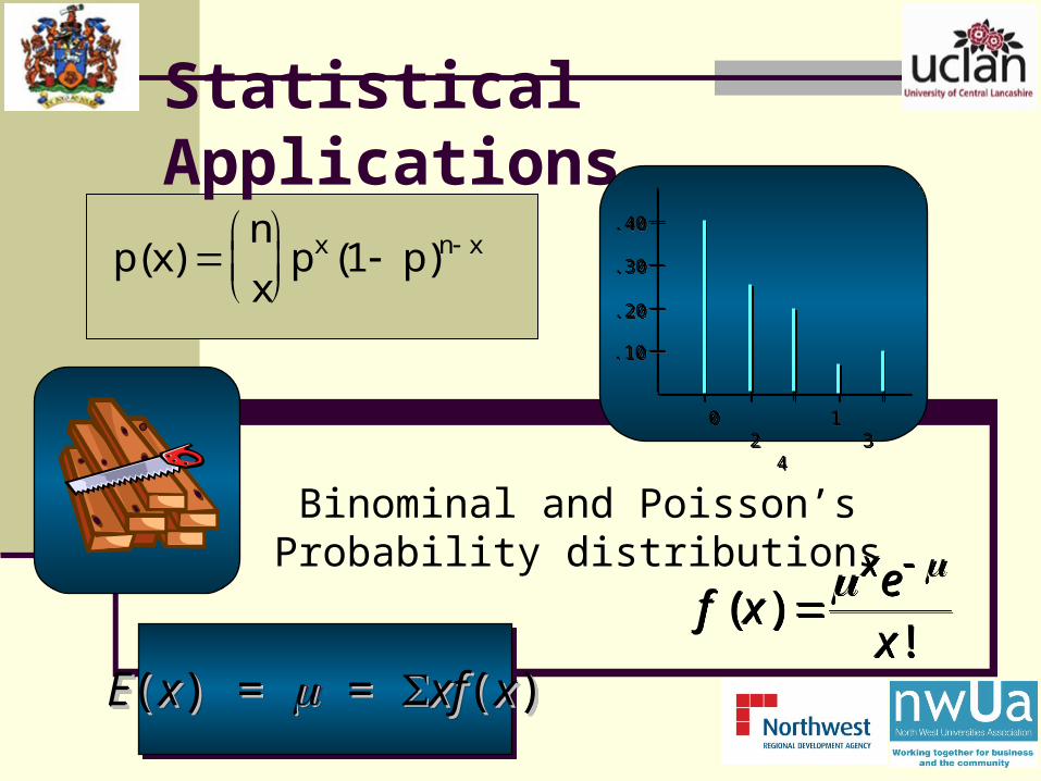
xx ff((xx)) 00 .40 .40 11 .25 .25 22 .20 .20 33 .05 .05 44 .10 .10

1.001.00

80/20080/200

Mean Value

The or mean or expected value, of a random variable

is a measure of its central location.

expected number expected number of TVs sold in a dayof TVs sold in a day

xx ff((xx)) xfxf((xx))

00 .40 .40 .00 .00

11 .25 .25 .25 .25

22 .20 .20 .40 .40

33 .05 .05 .15 .15

44 .10 .10 .40.40

EE((xx) = 1.20) = 1.20

EE((xx) = ) = = = xfxf((xx))EE((xx) = ) = = = xfxf((xx))

Mean cont…

• Graphical Representation of Probability Distribution

.10.10

.20.20

.30.30

.40.40

.50.50

0 1 2 3 40 1 2 3 4Values of Random Variable Values of Random Variable xx (TV sales) (TV sales)Values of Random Variable Values of Random Variable xx (TV sales) (TV sales)

Pro

babili

tyPro

babili

tyPro

babili

tyPro

babili

ty

Variance & Standard deviation

The variance summarizes the variability in the values of a random variable.

Var(Var(xx) = ) = 22 = = ((xx - - ))22ff((xx))Var(Var(xx) = ) = 22 = = ((xx - - ))22ff((xx))

NOTE: The NOTE: The standard deviationstandard deviation, , , is defined as the positive, is defined as the positive square root of the variance.square root of the variance. NOTE: The NOTE: The standard deviationstandard deviation, , , is defined as the positive, is defined as the positive square root of the variance.square root of the variance.

Binomial Distribution

• Four Properties of a Binomial Experiment

3. The probability of a success, denoted by 3. The probability of a success, denoted by pp, does, does not change from trial to trial.not change from trial to trial.3. The probability of a success, denoted by 3. The probability of a success, denoted by pp, does, does not change from trial to trial.not change from trial to trial.

4. The trials are independent.4. The trials are independent.4. The trials are independent.4. The trials are independent.

2. Two outcomes, 2. Two outcomes, successsuccess and and failurefailure, are possible, are possible on each trial.on each trial.2. Two outcomes, 2. Two outcomes, successsuccess and and failurefailure, are possible, are possible on each trial.on each trial.

1. The experiment consists of a sequence of 1. The experiment consists of a sequence of nn identical trials.identical trials.1. The experiment consists of a sequence of 1. The experiment consists of a sequence of nn identical trials.identical trials.

stationarystationaryassumptioassumptio

nn

• Of interest is the number of success occurring in n trials

• Let x be the number of successes

Binomial Probability Function

( )!( ) (1 )

!( )!x n xn

f x p px n x

( )!( ) (1 )

!( )!x n xn

f x p px n x

where:where: ff((xx) = the probability of ) = the probability of xx successes in successes in nn trials trials nn = the number of trials = the number of trials pp = the probability of success on any one trial = the probability of success on any one trial

Jacob Bernoulli

Binomial Probability Function cont…

• Evaluation of probabilities using the distribution function:

( )!( ) (1 )

!( )!x n xn

f x p px n x

( )!( ) (1 )

!( )!x n xn

f x p px n x

!!( )!

nx n x

!!( )!

nx n x

( )(1 )x n xp p ( )(1 )x n xp p

Probability of a particularProbability of a particular sequence of trial outcomessequence of trial outcomes with x successes in with x successes in nn trials trials

Probability of a particularProbability of a particular sequence of trial outcomessequence of trial outcomes with x successes in with x successes in nn trials trials

Number of experimentalNumber of experimental outcomes providing exactlyoutcomes providing exactly

xx successes in successes in nn trials trials

Number of experimentalNumber of experimental outcomes providing exactlyoutcomes providing exactly

xx successes in successes in nn trials trials

Binomial probability function alternative notation

• Evaluation of probabilities using the distribution function:

No of combinations

No of combinations

Notice the pattern of numbers

Notice the pattern of numbers

Probability of a particularProbability of a particular sequence of trial outcomessequence of trial outcomes with x successes in with x successes in nn trials trials

Probability of a particularProbability of a particular sequence of trial outcomessequence of trial outcomes with x successes in with x successes in nn trials trials

Number of experimentalNumber of experimental outcomes providing exactlyoutcomes providing exactly

xx successes in successes in nn trials trials

Number of experimentalNumber of experimental outcomes providing exactlyoutcomes providing exactly

xx successes in successes in nn trials trials

rnrr

n ppCrXP )1(

Mean and Variance

It is useful to note that for a binominal distribution the following are valid:

(1 )np p (1 )np p

EE((xx) = ) = = = npnp

Var(Var(xx) = ) = 22 = = npnp(1 (1 pp))

Expected Value

Variance

Standard Deviation

Example #1 :

Evans is concerned about a low retention rate for employees. In recent years, management has seen a turnover of 10% of the hourly employees annually. Thus, for any hourly employee chosen at random, management estimates a probability of 0.1 that the person will not be with the company next year.

Solution:

Using the Binomial Probability Function Choosing 3 hourly employees at random,

what is the probability that 1 of them will leave the company this year?

f xn

x n xp px n x( )

!!( )!

( )( )

1f xn

x n xp px n x( )

!!( )!

( )( )

1

1 23!(1) (0.1) (0.9) 3(.1)(.81) .243

1!(3 1)!f

1 23!

(1) (0.1) (0.9) 3(.1)(.81) .2431!(3 1)!

f

LetLet: p: p = 0.1, = 0.1, nn = 3, = 3, xx = 1 = 1

Exercise #1

A milling machine is know to produce 9% defective components, if a random sample of 5 components are taken, evaluate the probability of no more than 2 components being defective

Exercise #1: Solution

• Find the required parameters, namely:• p=0.09• n=5• X<3• Here you will need to use a little intelligence, i.e.:

pXXP )5,09.0Bi(|3

)Bi(0.09,5)2()Bi(0.09,5)1(

)Bi(0.09,5)0(

XXPXXP

XXPp

Now put the numbers into: f xn

x n xp px n x( )

!!( )!

( )( )

1f xn

x n xp px n x( )

!!( )!

( )( )

1

Exercise #1: Solution cont…

Using this standard formula gives

50 81.009.0)!5(!0

!5)0( XP

f xn

x n xp px n x( )

!!( )!

( )( )

1f xn

x n xp px n x( )

!!( )!

( )( )

1

Notice the pattern:Top and bottom equal the top4+1=5

41 81.009.0)!4(!1

!5)1( XP

586.0

043.01937.0349.0)2()1()0(

XPXPXP

32 81.009.0)!3(!2

!5)2( XP

Further example

A machine produces on average 1 defective parts out of 8. 5 samples are collected from this machine. Find the probability that 2 of them are defective.

pXXP )5,8/1Bi(|3

Solution:5 2 32( 2) (0.125) (1 0.125)

5!(0.015625)(0.669921875) 0.10475

2!3!

P X C

Notice here the new

nomenclature C2

5

Poisson’s distribution This distributions is named

after the famous French mathematician who formulated it:

Siméon Denis Poisson

A Poisson distributed random variable is oftenA Poisson distributed random variable is often useful in estimating the number of occurrencesuseful in estimating the number of occurrences over a over a specified interval of time or spacespecified interval of time or space

A Poisson distributed random variable is oftenA Poisson distributed random variable is often useful in estimating the number of occurrencesuseful in estimating the number of occurrences over a over a specified interval of time or spacespecified interval of time or space

It is a discrete random variable that may assumeIt is a discrete random variable that may assume an an infinite sequence of valuesinfinite sequence of values (x = 0, 1, 2, . . . ). (x = 0, 1, 2, . . . ). It is a discrete random variable that may assumeIt is a discrete random variable that may assume an an infinite sequence of valuesinfinite sequence of values (x = 0, 1, 2, . . . ). (x = 0, 1, 2, . . . ).

Poisson’s random variables

They can be time dependent or not!

Examples of a Poisson distributed random variable:Examples of a Poisson distributed random variable: Examples of a Poisson distributed random variable:Examples of a Poisson distributed random variable:

the number of knotholes in 14 linear feet ofthe number of knotholes in 14 linear feet of pine boardpine board the number of knotholes in 14 linear feet ofthe number of knotholes in 14 linear feet of pine boardpine board

the number of vehicles arriving at athe number of vehicles arriving at a toll booth in one hourtoll booth in one hour the number of vehicles arriving at athe number of vehicles arriving at a toll booth in one hourtoll booth in one hour

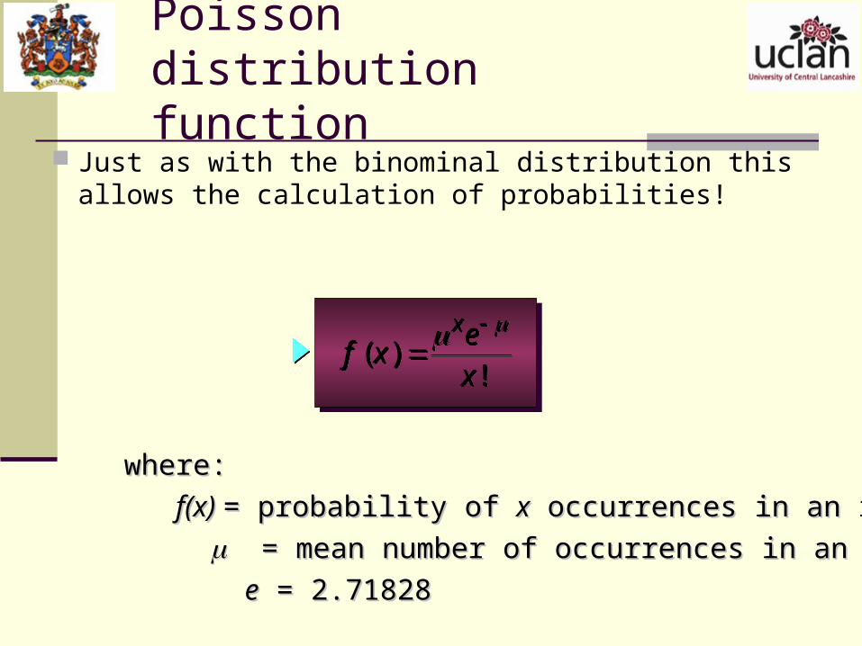
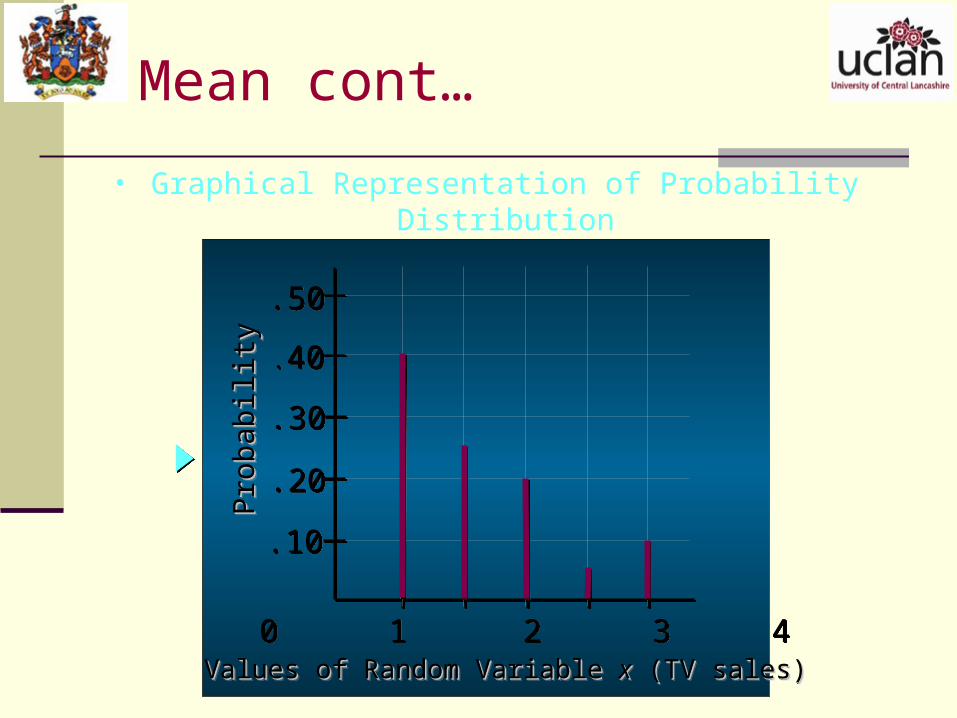
Poisson distribution function

Just as with the binominal distribution this allows the calculation of probabilities!

f xex

x( )

!

f x

ex

x( )

!

where:where:

f(x) f(x) = probability of = probability of xx occurrences in an interval occurrences in an interval

= mean number of occurrences in an interval= mean number of occurrences in an interval

ee = 2.71828 = 2.71828

Poisson’s cumulative distribution function

By definition this is given by:

)Po( XrXP

...!3!2!1!0

)Po(3210 eXrXP

Remembering this pattern helps in the evaluation of the required probabilities since each term in the series are respectively: P(X=0), P(X=1), P(X=2), P(X=3)

Example #2:

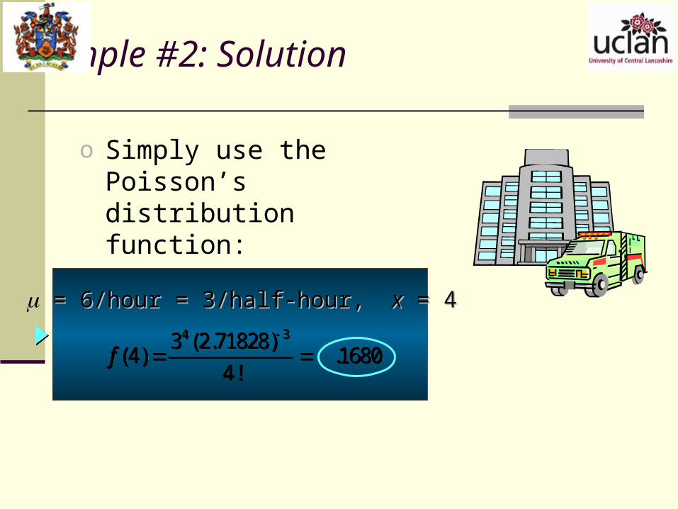
Patients arrive at the Casualty department of a hospital at the average rate of 6 per hour on weekend evenings. What is the probability of 4 arrivals in 30 minutes on a weekend evening?

Example #2: Solution

o Simply use the Poisson’s distribution function:

4 33 (2.71828)(4) .1680

4!f

4 33 (2.71828)

(4) .16804!

f

= 6/hour = 3/half-hour, = 6/hour = 3/half-hour, xx = 4 = 4

MERCYMERCY

Poisson’s distribution cont…

Poisson Distribution of ArrivalsPoisson Distribution of Arrivals

Poisson Probabilities

0.00

0.05

0.10

0.15

0.20

0.25

0 1 2 3 4 5 6 7 8 9 10Number of Arrivals in 30 Minutes

Pro

bab

ilit

y

NB: The Poisson’s distribution has the very special property of the mean and variance being equal!

= = 22

Also when n>50, i.e. large and np<5, i.e. small. Then this distribution approximates the Binominal.

Exercise #2:

A serviceman is “beeped” each time there is a call for service.

The number of beeps per hour is Poisson distributed with a

mean of 2 per hour. Find the probability that he gets beeped 3

times in the next 2 hours.

Solution: The units of interval need to be uniform. So, the mean beep rate will be 4 per 2 hour intervals.Application of the Poisson’s probability function, renders: 4 34 (0.0183)(64)

( 3) 0.1953! 6

eP X

Further Example

A garage workshop has an expensive machine tool which is used on

average 1.6 times per 8-hour day for a four hour period. How many

days in 60 day work period is the tool required no more than twice.

217.0258.0323.0202.01

1360217.0

)2()1()0(1 XPXPXPp

!2

6.1

!1

6.1

!0

6.11

2106.1e

Hence the required no. of days

Examination type questions

1. A machine is know to produce 10% defective components, if a random sample of 12 components are taken, evaluate the probability of:

a) No components being defective [2]

b) more than 3 components being defective [3]

2. If jobs arrive at a machine at random average intervals of 10/hr, estimate the probability of the machine remaining idle for a 1.5 hour period [4].

a) State the standard deviation of this distribution [1].

Further examination type questions

3. Over a long period of time it is known that 5% of the total production are below standard. If 6 are chosen at random, evaluate the probability that at least 2 are defective [5].

4. A machine is known to produce 2% defective components. In a packet of 100 what is the probability of obtaining over 2 defective components [5].

Solutions:

1. Here a simple application of the Binominal is required thus:

2. Here let X be a Poisson RV, thus:

2824.090.010.0)!12(!0

!12) 120 a

0852.02301.03765.02842.0

)9.0()1.0()9.0()1.0()9.0()1.0(2824.0) 933

121022

121111

12

CCCb

0!0

15

)15Po(0150

e

XXp

Solutions:

3. This is the binominal model:

4. We could use the binominal here but it is also a Poisson’s approximation with np=100×0.02, thus:

2321.07351.01)95.0()05.0(6)95.0(1

)95.0()05.0()95.0()05.0(1)1()0(1516

511

6600

6

CCXPXP

3233.051

!2

2211)2Po(21

2

22

e

eXXp

Alternative solution 4:

4. We could use the binominal here also, with n=100 and p=0.02:

3234.0

2734.02706.01326.01

)98.0()02.0()98.0()02.0(100)98.0(

)98.0()02.0()98.0()02.0()98.0()02.0(1

))100,02.0Bi(2(1

9822

100991100

9822

1009911

10010000

100

C

CCC

XXP

Note: It’s worth noticing the Poisson’s approximation if it turns up, “less calculations”!

Summary

Evaluate discrete probability distributions from realistic data

Use the binominal distribution to evaluate simple probabilities

Evaluate probabilities using the Poisson’s distribution

Answer examination type question pertaining to these distributions

Have we met out learning objectives? Specifically are you able to: