Embed Size (px)
Citation preview

Chapter 3
Poisson’s Equation
3.1 Physical Origins
Poisson’s equation,
∇2Φ = σ(x),
arises in many varied physical situations. Here σ(x) is the “source term”, and is often zero,
either everywhere or everywhere bar some specific region (maybe only specific points).
In this case, Laplace’s equation,
∇2Φ = 0,
results.
The Diffusion Equation
Consider some quantity Φ(x) which diffuses. (This might be say the concentration of
some (dilute) chemical solute, as a function of position x, or the temperature T in some
heat conducting medium, which behaves in an entirely analogous way.) There is a cor-
responding flux, F, of Φ – that is, the amount crossing an (imaginary) unit area per
unit time. Experimentally, it is known that, in the case of a solute, the flux is given by
F = −k∇Φ where k is the diffusivity ; in the case of temperature, the flux of heat is given
by F = −k∇T where k is the coefficient of heat conductivity. (Note that the minus sign
occurs because the flux is directed towards regions of lower concentration.)
38

The governing equation for this diffusion process is
∂Φ
∂t= k∇2Φ
where k is referred to, generically, as the diffusion constant. If we are interested in
the steady-state distribution of solute or of temperature, then ∂Φ/∂t = 0 and Laplace’s
equation, ∇2Φ = 0, follows.
When there are sources S(x) of solute (for example, where solute is piped in or where
the solute is generated by a chemical reaction), or of heat (e.g., an exothermic reaction),
the steady-state diffusion is governed by Poisson’s equation in the form
∇2Φ = −S(x)
k.
The diffusion equation for a solute can be derived as follows. Let Φ(x) be the concentration of solute atthe point x, and F(x) = −k∇Φ be the corresponding flux. (We assume here that there is no advectionof Φ by the underlying medium.)
Let V be a fixed volume of space enclosed by an (imaginary) surface S. In a small time δt, the quantityof solute leaving V is given by
∫∫
S
Fδt . n dS.
Hence[∫∫∫
V
Φ dV
]t+δt
t
= −∫∫
S
F . n dS δt.
Dividing by δt and taking the limit as δt → 0,
d
dt
∫∫∫
V
Φ dV = −∫∫
S
F . n dS =
∫∫
S
k∇Φ . n dS,
and hence by the Divergence Theorem,
∫∫∫
V
∂Φ
∂tdV =
∫∫∫
V
∇ . (k∇Φ)dV.
39
As this is true for any fixed volume V , we must have
∂Φ
∂t= ∇ . (k∇Φ)
everywhere. Assuming that k is constant, we obtain the diffusion equation
∂Φ
∂t= k∇2Φ.
If there are also sources (or sinks) of solute, then an additional source term results:
∂Φ
∂t= k∇2Φ + S(x)
where S(x) is the quantity of solute (per unit volume and time) being added to the solution at thelocation x. Poisson’s equation for steady-state diffusion with sources, as given above, follows immediately.
The heat diffusion equation is derived similarly. Let T (x) be the temperature field in some substance(not necessarily a solid), and H(x) the corresponding heat field. We have the relation H = ρcT whereρ is the density of the material and c its specific heat. The corresponding heat flux is −k∇T . A similarargument to the above applies again, resulting in
∂H
∂t= k∇2T + S(x)
where S represents possible sources of heat. Hence
∂T
∂t= κ∇2T + (ρc)−1S(x)
where κ = k/ρc is the coefficient of thermal diffusivity. The equation for steady-state heat diffusion withsources is as before.
Electrostatics
The laws of electrostatics are
∇ . E = ρ/ǫ0 ∇×E = 0
∇ . B = 0 ∇×B = µ0J
where ρ and J are the electric charge and current fields respectively. Since ∇ × E = 0,
there is an electric potential Φ such that E = −∇Φ; hence ∇ . E = ρ/ǫ0 gives Poisson’s
equation
∇2Φ = −ρ/ǫ0.
In a region where there are no charges or currents, ρ and J vanish. Hence we obtain
Laplace’s equation
∇2Φ = 0.
Also ∇×B = 0 so there exists a magnetostatic potential ψ such that B = −µ0∇ψ; and
∇2ψ = 0.
40
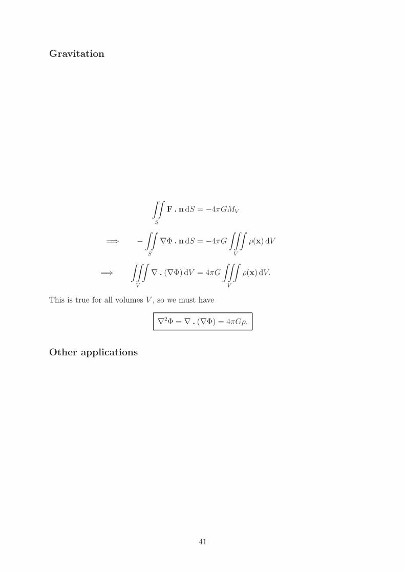
Gravitation
Consider a mass distribution with density ρ(x). There is a corre-
sponding gravitational field F(x) which we may express in terms of
a gravitational potential Φ(x). Consider an arbitrary fixed volume
V with surface S containing a total mass MV =∫∫∫
V ρ(x) dV .
Gauss showed that the flux of the gravitational field through S is
equal to −4πGMV . Hence
∫∫
S
F . n dS = −4πGMV
=⇒ −∫∫
S
∇Φ . n dS = −4πG
∫∫∫
V
ρ(x) dV
=⇒∫∫∫
V
∇ . (∇Φ) dV = 4πG
∫∫∫
V
ρ(x) dV.
This is true for all volumes V , so we must have
∇2Φ = ∇ . (∇Φ) = 4πGρ.
Other applications
These include the motion of an inviscid fluid; Schrodinger’s equa-
tion in Quantum Mechanics; and the motion of biological organ-
isms in a solution.
41

3.2 Separation of Variables for Laplace’s Equation
Plane Polar Coordinates
We shall solve Laplace’s equation ∇2Φ = 0 in plane polar coordinates (r, θ) where the
equation becomes1
r
∂
∂r
(
r∂Φ
∂r
)
+1
r2
∂2Φ
∂θ2= 0. (1)
Consider solutions of the form Φ(r, θ) = R(r)Θ(θ) where each function R, Θ is a function
of one variable only. Then
1
r
∂
∂r
(
r∂Φ
∂r
)
=Θ(θ)
r
d
dr
(
rdR
dr
)
and1
r2
∂2Φ
∂θ2=R(r)
r2
d2Θ
dθ2.
Hence after rearrangement,r
R
d
dr
(
rdR
dr
)
= −Θ′′
Θ. (2)
The LHS is a function of r only, and the RHS of θ only; hence both must be constant, λ
say. Then
Θ′′ = −λΘ
=⇒ Θ =
A+Bθ λ = 0
A cos√λ θ +B sin
√λ θ λ 6= 0
To obtain a sensible physical solution, replacing θ by θ + 2π should give the same value
of ∇Φ (see later). This is true only if Θ′(θ + 2π) = Θ′(θ) ∀ θ; i.e., either λ = 0 or
cos 2π√λ = 1 and sin 2π
√λ = 0
which implies 2π√λ = 2nπ for some integer n. (Note that the possibility that λ < 0 is
ruled out at this stage.) Hence
Θ =
A +Bθ n = 0
A cosnθ +B sinnθ n 6= 0
42

Returning to (2),
r
R
d
dr
(
rdR
dr
)
= λ = n2
=⇒ r2R′′ + rR′ − n2R = 0.
It is easily shown (either by direct verification or by making the
substitution u = ln r) that the solutions of this equation are
R =
C +D ln r n = 0
Crn +Dr−n n 6= 0
Hence, we obtain possible solutions to (1) as
Φ = RΘ =
(C +D ln r)(A+Bθ) n = 0
(Crn +Dr−n)(A cosnθ +B sin nθ) n 6= 0
We note that the combination θ ln r does not satisfy the requirement above for 2π-
periodicity of ∇Φ, and so we exclude it. Equation (1) is linear and so we may form
a superposition of the above solutions; in fact the general solution is an arbitrary linear
combination of all the possible solutions obtained above, that is
Φ = A0 +B0θ + C0 ln r +∞
∑
n=1
(Anrn + Cnr
−n) cosnθ +∞
∑
n=1
(Bnrn +Dnr
−n) sinnθ
where we have relabelled all the arbitrary constants, e.g., AC has become An and BD
has become Dn. We can make this expression more compact by defining A−n = Cn and
B−n = Dn for n > 0; then
Φ = A0 +B0θ + C0 ln r +
∞∑
n=−∞
n 6=0
rn(An cosnθ +Bn sinnθ).
Although this is more compact, the first expression is often easier to use.
43
Notes:
(i) Why did we require that ∇Φ, rather than Φ itself, be periodic?
In many cases (e.g. temperature, diffusion), Φ must clearly be
periodic and so we shall further need B0 = 0. But in other
cases (e.g. electrostatics, gravitation), Φ is not itself a physi-
cal quantity, only a potential; it is ∇Φ which has a physical
significance (e.g., the force). For example, consider the mag-
netostatic potential around a wire carrying a current I ; here
ψ = −(I/2π)θ, which is multi-valued, but B = −µ0∇ψ (the
quantity of physical interest) is of magnitude µ0I/2πr and is
single valued.
(ii) A common mistake made during separation of variables is to retain too many arbi-
trary constants; e.g. to write
∑
Cnrn(An cos nθ +Bn sinnθ).
For each n, this looks like 3 arbitrary constants (An, Bn, Cn); but of course there
are really only two arbitrary quantities (CnAn and CnBn, which we have relabelled
as An and Bn above).
(iii) The above derivation also applies to 3D cylindrical polar coordinates in the case
when Φ is independent of z.
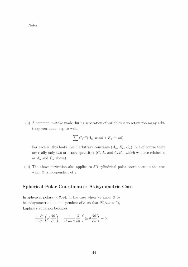
Spherical Polar Coordinates: Axisymmetric Case
In spherical polars (r, θ, φ), in the case when we know Φ to
be axisymmetric (i.e., independent of φ, so that ∂Φ/∂φ = 0),
Laplace’s equation becomes
1
r2
∂
∂r
(
r2∂Φ
∂r
)
+1
r2 sin θ
∂
∂θ
(
sin θ∂Φ
∂θ
)
= 0.
44
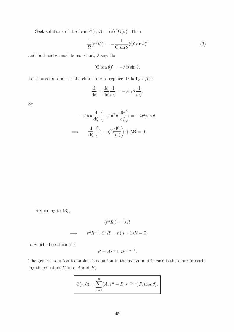
Seek solutions of the form Φ(r, θ) = R(r)Θ(θ). Then
1
R(r2R′)′ = − 1
Θ sin θ(Θ′ sin θ)′ (3)
and both sides must be constant, λ say. So
(Θ′ sin θ)′ = −λΘ sin θ.
Let ζ = cos θ, and use the chain rule to replace d/dθ by d/dζ :
d
dθ=
dζ
dθ
d
dζ= − sin θ
d
dζ.
So
− sin θd
dζ
(
− sin2 θdΘ
dζ
)
= −λΘ sin θ
=⇒ d
dζ
(
(1 − ζ2)dΘ
dζ
)
+ λΘ = 0.
This is Legendre’s equation; for well-behaved solutions at ζ =
±1 (i.e., θ = 0, π) we need λ = n(n + 1) for some non-negative
integer n, in which case
Θ = CPn(ζ) = CPn(cos θ)
where C is an arbitrary constant.
Returning to (3),
(r2R′)′ = λR
=⇒ r2R′′ + 2rR′ − n(n + 1)R = 0,
to which the solution is
R = Arn +Br−n−1.
The general solution to Laplace’s equation in the axisymmetric case is therefore (absorb-
ing the constant C into A and B)
Φ(r, θ) =
∞∑
n=0
(Anrn +Bnr
−n−1)Pn(cos θ).
45

Non-axisymmetric Case [non-examinable]
A similar analysis when Φ may depend on φ shows that the general solution is
Φ(r, θ, φ) =
∞∑
n=0
n∑
m=−n
(Amnrn + Bmnr−n−1)Pmn (cos θ)eimφ
where Pmn (ζ) are the associated Legendre functions which satisfy the associated Legendre equation
d
dζ
(
(1 − ζ2)dΘ
dζ
)
+
(
n(n + 1) +m
1 − ζ2
)
Θ = 0
when m and n are integers, n ≥ 0, −n ≤ m ≤ n.
3.3 Uniqueness Theorem for Poisson’s Equation
Consider Poisson’s equation
∇2Φ = σ(x)
in a volume V with surface S, subject to so-called Dirichlet boundary conditions Φ(x) =
f(x) on S, where f is a given function defined on the boundary.
From a physical point of view, we have a well-defined problem;
say, find the steady-state temperature distribution throughout V ,
with heat sources given by σ(x), subject to a specified temperature
distribution on the boundary. No further conditions are required in
real life to ensure that there is only one solution. Mathematically,
then, can we show that the problem above has a unique solution?
Suppose that there are actually two (or more) solutions Φ1(x) and Φ2(x). Let Ψ =
Φ1 − Φ2. Then
∇2Ψ = ∇2Φ1 −∇2Φ2 = σ − σ = 0 in V
subject to
Ψ = f − f = 0 on S.
One solution of this problem for Ψ is clearly Ψ = 0; is it unique? Consider
∇ . (Ψ∇Ψ) = ∇Ψ . ∇Ψ + Ψ∇ . (∇Ψ)
= |∇Ψ|2 + Ψ∇2Ψ
= |∇Ψ|2.
46

Hence∫∫∫
V
|∇Ψ|2 dV =
∫∫∫
V
∇ . (Ψ∇Ψ) dV
=
∫∫
S
Ψ∇Ψ . n dS
= 0
because Ψ = 0 on S. But |∇Ψ|2 ≥ 0 everywhere; its integral can only be zero if |∇Ψ|is zero everywhere, i.e., ∇Ψ ≡ 0, which implies that Ψ is constant throughout V . But
Ψ = 0 on S, so Ψ ≡ 0 throughout V . Thus Φ1 = Φ2, which demonstrates that our
problem has a unique solution, as expected.
A similar theorem holds when instead of Dirichlet boundary conditions we have Neu-
mann boundary conditions: that is to say instead of Φ being specified (by the function
f) on the boundary S, ∂Φ/∂n is specified on S, where we use the notation
∂Φ
∂n≡ n . ∇Φ.
3.4 Minimum and Maximum Properties of Laplace’s
Equation
Suppose that Φ satisfies ∇2Φ = 0 in a volume V with surface S. Let m be the minimum
value of Φ on S, and M be the maximum value of Φ on S. Then either m = M and Φ
is constant everywhere in V (including S) (with Φ = m = M), or m < Φ < M in V − S
(where V − S denotes V excluding S).
Why might we expect this? Suppose Φ has a local maximum
somewhere in the interior of V . At that point we must have
∂Φ/∂x = ∂Φ/∂y = ∂Φ/∂z = 0 (stationary point).
Suppose it is a maximum with ∂2Φ/∂x2 < 0, ∂2Φ/∂y2 <
0, ∂2Φ/∂z2 < 0. But this cannot happen since 0 = ∇2Φ =
∂2Φ/∂x2 + ∂2Φ/∂y2 + ∂2Φ/∂z2.
This does not constitute a full proof since it is actually possible
47

for a maximum to have
∂2Φ
∂x2=∂2Φ
∂y2=∂2Φ
∂z2= 0,
a case we haven’t considered: compare with the possibility in 1D
that a maximum could have d2y/dx2 = 0.
For a full proof, first let VR denote the sphere of radius R > 0, centred at the origin, with surface SR,and suppose that Φ is harmonic on VR. Then for r such that 0 < r < R, define
g(r) =
∫∫
Sr
Φ dS =
∫ 2π
0
∫ π
0
r2Φ(rer) sin θdθdφ .
Then it is straightforward to show, using the chain rule, that
d
dr(r−2g(r)) =
∫ 2π
0
∫ π
0
er · ∇Φ sin θdθdφ =1
r2
∫∫
Sr
∂Φ
∂ndS =
1
r2
∫∫∫
V
∇2Φ dV = 0 ,
using the divergence theorem, together with ∇2Φ = 0. So r−2g(r) is constant.
It follows that
g(r)
r2= lim
r→0
∫ 2π
0
∫ π
0
Φ(rer) sin θdθdφ = 4πΦ(0) ,
which in turn implies
∫∫
Sr
Φ dS = 4πr2Φ(0) .
Also, we find
∫∫∫
Vr
Φ dV =
∫ r
0
g(r′)dr′ =
∫ r
0
4π(r′)2Φ(0)dr′ =4
3πr3Φ(0) .
More generally, this implies that if Φ satisfies ∇2Φ = 0 on a sphere Vr, of radius r, centre x0, then
Φ(x0) =1
Vol(Vr)
∫∫∫
Vr
Φ dV (1) .
Now return to the original problem. Suppose that M denotes the maximum of Φ on V (including S).Also suppose that there is some point x0 ∈ V , x0 /∈ S such that Φ(x0) = M . Then for sufficiently smallr, there exists a sphere Vr, centred on x0 such that Vr lies entirely in V .
Suppose that there exists some y0 ∈ Vr with Φ(y0) < Φ(x0). Then (1) implies that
48

M = Φ(x0) =1
Vol(Vr)
∫∫∫
Vr
Φ dV .
But because Φ(y0) < Φ(x0), it must also be the case that∫∫∫
Vr
Φ dV < MVol(Vr), in contradiction to the
above expression. So Φ = M everywhere in Vr. Assuming that Φ is sufficiently smooth in V , this impliesthat Φ = M everywhere in V .
Therefore, either the maximum of Φ occurs on the boundary of V , or Φ is constant on V . A similarargument applied to the minimum value of Φ also shows that the minimum of Φ occurs on the boundaryof V , or Φ is constant on V . This establishes the result.
The proof relies implicitly on certain properties of the topology of V and of the degree
to which Φ is smooth in V - we shall not elaborate on this any further here.
Example: in the worked example of the steady-state temperature distribution in a
cylinder, we note that |T | ≤ T0 in r < a.
3.5 Green’s Function
The Delta Function in 3D
In 1D, δ(x − x0) is a function which is zero everywhere except at x = x0, and is infinite
there in such a way that∫ b
a
δ(x− x0) dx = 1
whenever x0 ∈ (a, b). As a consequence,∫ b
af(x)δ(x − x0) dx = f(x0). We extend the
definition to 3D via
δ(x − x0) = δ(x− x0)δ(y − y0)δ(z − z0)
where x0 = (x0, y0, z0). Then
∫∫∫
V
f(x)δ(x − x0) dV = f(x0)
whenever x0 ∈ V (and the integral is 0 otherwise).
49
Green’s Function
Suppose that we wish to solve Poisson’s equation in a volume V with surface S on which
Dirichlet boundary conditions are imposed. The Green’s function G(x;x0) associated
with this problem is a function of two variables: x, the position vector, and x0, a fixed
location. It is defined as the solution to
∇2G(x;x0) = δ(x − x0) in V ,
G = 0 on S.
(Physically, we can think of G as the “potential” from a point source at x0 with the
boundary held at zero potential.)
It is possible to prove that G is symmetric, i.e., G(x;x0) = G(x0;x). This can be useful as a check thatG has been correctly calculated. Physically, this corresponds to the remarkable fact that the potentialat x due to a source at x0 is the same as the potential at x0 due to a source at x, regardless of the shapeof S.
When V is all space (i.e., the limit of a sphere whose radius tends to ∞), Green’s
function is known as the fundamental solution.
For a problem with Neumann boundary conditions, G(x;x0) is
defined to satisfy ∂G/∂n = 1/A on S, where A =∫∫
S dS is the
surface area of S, rather than G = 0 there. In many cases S is
infinitely large, in which case the boundary condition reduces to
∂G/∂n = 0.
50

The Fundamental Solution in 3D
Consider first x0 = 0. Then ∇2G = δ(x) and G → 0 as |x| → ∞. The problem is
spherically symmetric about the origin, so we expect G to be a function of r alone. Try
G = g(r). By the definition of δ(x), if VR is the sphere of radius R with surface SR,
1 =
∫∫∫
VR
δ(x) dV =
∫∫∫
VR
∇ . (∇G) dV
=
∫∫
SR
∇G . n dS =
∫∫
SR
g′(R) dS
(n is just the unit radial vector)
= g′(R)
∫∫
SR
dS = 4πR2g′(R)
=⇒ g′(R) =1
4πR2for all R
=⇒ g′(r) =1
4πr2
=⇒ g(r) = − 1
4πr+ A,
where A is a constant. As r → ∞, G→ 0, so A = 0. Hence the solution is −1/4π|x|.
Shifting the origin to a non-zero x0, we see that in general the fundamental solution
in 3D is
G(x;x0) = − 1
4π|x − x0|.
Example: an electron located at x0 is an electrostatic point source, so the charge
distribution in space is ρ(x) = −e δ(x − x0). Hence the electrostatic potential obeys
∇2Φ = (e/ǫ0) δ(x − x0)
using a result from §3.1. The solution Φ is therefore just a factor e/ǫ0 times the funda-
mental solution, i.e., −e/4πǫ0|x−x0|. This is the standard formula for the potential due
to an electron.
51
The Fundamental Solution in 2D
Again, we solve ∇2G = δ(x), where the delta-function is now
in 2D. We will see that a solution with G → 0 as |x| → ∞ is
impossible; instead we will find a solution such that |∇G| → 0.
As before, G = g(r) (where r is now the plane polar radius). Applying the Divergence
Theorem in 2D to a circle of radius R,
1 =
∫∫
r≤R
δ(x) dV =
∫∫
r≤R
∇ . (∇G) dV
=
∮
r=R
∇G . n dl =
∮
r=R
g′(r) dl
= 2πRg′(R)
=⇒ g′(r) =1
2πr
=⇒ g(r) =1
2πln r + constant.
(Note that g′(r) → 0 as r → ∞, but g(r) → ∞, whatever the constant.)
Shifting the origin, we see that the fundamental solution in 2D is
G(x;x0) =1
2πln |x − x0| + constant.
Example: consider an infinitely long charged wire in three dimensions lying along the
z-axis, with a charge density of µ per unit length. What is the electric potential Φ around
the wire?
We assume the wire to be mathematically perfect, i.e., of infinitesimal width. Then
the electric charge distribution, in 3D, is ρ = µδ(x)δ(y). (Check that this gives the
correct result for the amount of charge in a unit length of the wire.) But it is clear
that this problem is fundamentally two-dimensional, with ρ = µδ(x) where x = (x, y);
and the potential satisfies ∇2Φ = −µδ(x)/ǫ0. Hence the potential is (up to an arbi-
trary additional constant) just given by an appropriate multiple of the two-dimensional
fundamental solution, namely
Φ = − µ
2πǫ0ln |x| = − µ
2πǫ0ln
√
x2 + y2 = − µ
2πǫ0ln r
where r is the perpendicular distance to the wire (i.e., the “r” of cylindrical polar coor-
dinates rather than of spherical polars).
52

3.6 The Method of Images
We can use the fundamental solution to find Green’s function in
some simple geometries, using the “method of images”. We shall
find a function which satisfies the equation and the boundary con-
ditions; by uniqueness, this must be the Green’s function.
Example: A 3D half-space x > 0
Suppose that the domain D is the half-space of R3 with x > 0. The
Green’s function obeys
∇2G = δ(x − x0) ∀x ∈ D,
G = 0 on x = 0,
G→ 0 as |x| → ∞, x ∈ D.
Consider the solution in all space for the point source at x = x0
(with x0 = (α, β, γ), α > 0), together with another (imaginary)
source of strength −1 at the “image point” x = x1 as shown (with
x1 = (−α, β, γ)):
Φ = − 1
4π|x − x0|− −1
4π|x− x1|
and
∇2Φ = δ(x − x0) − δ(x − x1)
by superposition of the two fundamental solutions. This certainly satisfies the require-
ment ∇2Φ = δ(x − x0) for all x ∈ D, because δ(x − x1) ≡ 0 ∀x ∈ D. It also satisfies
Φ → 0 as |x| → ∞; and on x = 0, |x−x0| = |x−x1| so that Φ = 0. Hence by uniqueness,
G(x;x0) = Φ = − 1
4π
(
1
|x − x0|− 1
|x − x1|
)
.
53

Example: A 2D quarter-plane x > 0, y > 0
In this case, we need to find G such that
∇2G = δ(x − x0) ∀x ∈ D
with G = 0 on both x = 0 and y = 0. We find that we need 3 image sources as
shown: x1 and x2 with strength −1, and x3 with strength +1 (taking x0 = (α, β),x1 =
(−α, β), x2 = (α,−β), x3 = (−α,−β) for α > 0, β > 0) . Then
G =1
2πln |x − x0| −
1
2πln |x − x1| −
1
2πln |x − x2| +
1
2πln |x − x3| + constant
=1
2πln
|x − x0| |x − x3||x − x1| |x − x2|
+ constant.
Clearly ∇2G = δ(x − x0) in D (all the other delta-functions are zero there); on x = 0,
|x−x0| = |x−x1| and |x−x2| = |x−x3|, so choosing the constant to be zero ensures that
G = 0; similarly on y = 0. By uniqueness, then, this is the required Green’s function.
Further extensions to this idea are possible; e.g., planes inclined
at 60◦ to each other, or a pair of parallel planes.
54

Example: Heat flow from a source in a 3D half-space with a wall at constant
temperature
Suppose that the ambient temperature is T0 and that
a wall at x = 0 is held at that temperature, with a
heat source of strength Q at x0. Then
T = T0 −Q
kG(x;x0),
where G is the Green’s function for the 3D half-space
x > 0. (Why? Because we need to solve ∇2T =
−Q
kδ(x−x0) here, with T = T0 at infinity and on the
wall.)
What is the total heat flux across the wall S? It is∫∫
S
(−k∇T ) . n dS = k
∫ ∞
−∞
∫ ∞
−∞
∂T
∂xdy dz = −Q
∫ ∞
−∞
∫ ∞
−∞
∂
∂xG(x;x0)
∣
∣
∣
∣
x=0
dy dz
which we can evaluate (see the worked example in the next section for an example of this
sort of evaluation).
Alternatively, we can use the Divergence Theorem on the surface consisting of the
wall S, plus the hemisphere H at ∞.∫∫
H
(−k∇T ) . n dS +
∫∫
S
(−k∇T ) . n dS = −∫∫∫
V
∇ . (k∇T ) dV
= −k∫∫∫
V
∇2T dV
= −k∫∫∫
V
(
−Qkδ(x − x0)
)
dV
= Q,
In order to compute the contribution from the hemisphere, note that
T = T0 +Q
4πk
( 1
|x − x0|− 1
|x − x1|)
where if x0 = (α, β, γ) for α > 0, then x1 = (−α, β, γ) is the “image point”. Hence
T = T0 + O(r−2) at infinity (which should be checked!). Therefore ∇T falls-off as r−3
at infinity, whereas the surface element dS grows only as r2. So, the contribution to the
flux integral from the hemisphere at infinity vanishes and the total heat flux across the
wall is Q.
55

Example: A point charge near an earthed boundary plate
Here
Φ = − e
ǫ0G(x;x0)
where G is the Green’s function for the 3D half-space x > 0.
Now the surface charge density induced on the plate is µ = ǫ0Ex (standard result from electrostatics,where Ex is the x-component of E). The normal force (per unit area) on the plate, towards the charge,is
1
2µEx = 1
2ǫ0E
2x = 1
2ǫ0
(
−∂Φ
∂x
)2
=e2
2ǫ0
(
∂G
∂x
)2
,
and we calculate ∂G/∂x as in the worked example in the next section. We can integrate this over thewhole plate to obtain the total force:
e2
2ǫ0
∫
∞
−∞
∫
∞
−∞
x20
4π2(
x20 + (y − y0)2 + (z − z0)2
)3dy dz = · · · =
e2
16πǫ0x20
.
The force on the charge from the plate is equal and opposite, i.e., e2/4πǫ0(2x0)2 towards the wall. Note
that we could also have found this directly by considering the force on the charge due to the imagecharge, ignoring the plate!
Example: Images in a sphere
What is Green’s function for the domain r < a in 3D? We need
∇2G = δ(x − x0) in r < a,
G = 0 on r = a.
The image point turns out to be at the inverse point
x1 =a2
|x0|2x0
(so that a/|x1| = |x0|/a) with strength −a/|x0|, so Green’s function is
G(x;x0) =1
4π
(
− 1
|x − x0|+
a/|x0||x − x1|
)
.
(Check this by first showing that |x − x1|2 = (x − x1) . (x − x1) = (a2/|x0|2)|x − x0|2when |x| = a.)
Note that the same result holds if we consider the domain r > a instead.
56

Example: Images in a circle
This is the 2D equivalent of the above. The image point is at
x1 = (a2/|x0|2)x0 as before, but now the strength of the image is
just −1, so the Green’s function is
G(x;x0) =1
2πln |x − x0| −
1
2πln |x − x1| + constant
=1
2πln|x − x0||x − x1|
+ constant.
Choosing the constant correctly, we can ensure that G = 0 on the
circle r = a.
3.7 The Integral Solution of Poisson’s Equation
The most important application of Green’s function is that it can be used to find the
solution of Poisson’s equation with an arbitrary source distribution.
Green’s Identity
For any smooth functions Φ and Ψ, Green’s Identity is
∫∫∫
V
(Φ∇2Ψ − Ψ∇2Φ) dV =
∫∫
S
(Φ∇Ψ − Ψ∇Φ) . n dS
where V is a volume with surface S. This is proved by applying the Divergence Theorem
to the vector field F = Φ∇Ψ − Ψ∇Φ, and using ∇ . (Φ∇Ψ) = ∇Φ . ∇Ψ + Φ∇2Ψ.
The RHS is also written∫∫
S
(
Φ∂Ψ
∂n− Ψ
∂Φ
∂n
)
dS.
57

The Integral Solution
Consider the general problem of Poisson’s equation with Dirichlet boundary conditions:
∇2Φ = σ in V ,
Φ = f on S.
Apply Green’s Identity, taking Ψ to be the Green’s function G(x;x0) for the problem:∫∫∫
V
(Φ∇2G−G∇2Φ) dV =
∫∫
S
(Φ∇G−G∇Φ) . n dS
δ(x − x0) σ f 0
=⇒∫∫∫
V
Φδ(x − x0) dV =
∫∫∫
V
Gσ dV +
∫∫
S
f∂G
∂ndS
=⇒ Φ(x0) =
∫∫∫
V
σ(x)G(x;x0) dV +
∫∫
S
f(x)∂G
∂ndS.
This is the Integral Solution of Poisson’s equation.
Notes:
(i) We can also use the integral solution to solve Laplace’s equation with Dirichlet
boundary conditions, by taking σ(x) = 0.
(ii) A similar result (but with technical differences) can be derived for Neumann bound-
ary conditions, in which case G is defined differently (see §3.5).
(iii) We sometimes wish to take V to be “all space”, by taking
the limit of a sphere whose radius tends to ∞. In this case
we simply use the fundamental solution for G; but (strictly
speaking) we need to ensure that the surface integral tends
to zero (by requiring, for example, that on the surface of the
sphere, Φ(x) → 0 sufficiently quickly as the radius increases).
Then
Φ(x0) =
∫∫∫
R3
σ(x)G(x;x0) dV.
58
This latter result is easy to understand in many physical situations. For instance,
consider an arbitrary electrostatic charge distribution ρ(x). Then
∇2Φ = −ρ/ǫ0 in R3,
Φ → 0 as |x| → ∞.
(We assume here that the charge distribution decays rapidly far from the origin.) Us-
ing the integral solution of Poisson’s equation, with V = R3, and setting G to be the
fundamental solution in 3D,
Φ(x0) =
∫∫∫
R3
ρ(x)
4πǫ0|x − x0|dV.
We can interpret this physically as the superposition of many infinitesimal charge elements
ρ(x) dV . Each of these is effectively a point charge, and the potential at x0 from such
a point charge (using the standard formula for the electrostatic potential due to a point
charge) is just ρ(x) dV/4πǫ0|x − x0|. Summing over all such infinitesimal elements gives
the above result.
59