Stateless Core: A Scalable Approach for Quality ofService in the Internet

Ion Stoica

December 15, 2000

CMU-CS-00-176

Department of Electrical and Computer EngineeringCarnegie Mellon University

Pittsburgh, PA 15213

Thesis Committee:Hui Zhang, ChairGarth A. GibsonThomas Gross

Peter SteenkisteScott Shenker, ICSI Berkeley

Submitted in partial fulfillment of the requirements forthe degree of Doctor of Philosophy

Copyright c�

2000 by Ion Stoica

This research was sponsored by DARPA under contract numbers N66001-96-C-8528, E30602-97-2-0287, andDABT63-94-C-0073. Additional support was provided by Intel Corp., MCI, and Sun Microsystems.

Views and conclusions contained in this document are those of the authors and should no be interpreted as repre-senting the official policies, either expressed or implied, of DARPA, NSF, Intel, MCI, Sun, or the U.S. government.

Keywords: Quality of Service, Internet, scalabile networks, stateless core, support for conges-tion control, Differentiated Services, Intergated Services

Abstract

Today’s Internet provides one simple service: best effort datagram delivery. This minimalist serviceallows the Internet to be stateless, that is, routers do not need to maintain any fine grained informa-tion about traffic. As a result of this stateless architecture, the Internet is both highly scalable androbust. However, as the Internet evolves into a global commercial infrastructure that is expectedto support a plethora of new applications such as IP telephony, interactive TV, and e-commerce,the existing best effort service will no longer be sufficient. In consequence, there is an urgent needto provide more powerful services such as guaranteed services, differentiated services, and flowprotection.

Over the past decade, there has been intense research toward achieving this goal. Two classes ofsolutions have been proposed: those maintaining the stateless property of the original Internet (e.g.,Differentiated Services), and those requiring a new stateful architecture (e.g., Integrated Services).While stateful solutions can provide more powerful and flexible services such as per flow bandwidthand delay guarantees, they are less scalable than stateless solutions. In particular, stateful solutionsrequire each router to maintain and manage per flow state on the control path, and to perform perflow classification, scheduling, and buffer management on the data path. Since today’s routers canhandle millions of active flows, it is difficult, if not impossible, to implement such solutions in ascalable fashion. On the other hand, while stateless solutions are much more scalable, they offerweaker services.

The key contribution of this dissertation is to bridge this long-standing gap between statelessand stateful solutions in packet switched networks such as the Internet. Our thesis is that “it isactually possible to provide services as powerful and as flexible as the ones implemented by astateful network using a stateless network”. To prove this thesis, we propose a novel techniquecalled Dynamic Packet State (DPS). The key idea behind DPS is that, instead of having routersmaintain per flow state, packets carry the state. In this way, routers are still able to process packetson a per flow basis, despite the fact that they do not maintain any per flow state. Based on DPS,we develop a network architecture called Stateless Core (SCORE) in which core routers do notmaintain any per flow state. Yet, using DPS to coordinate actions of edge and core routers alongthe path traversed by a flow allows us to design distributed algorithms that emulate the behavior ofa broad class of stateful networks in SCORE networks.

In this dissertation we describe complete solutions including architectures, algorithms and im-plementations which address three of the most important problems in today’s Internet: providingguaranteed services, differentiated services, and flow protection. Compared to existing solutions,our solutions eliminate the most complex operations on both the data and control paths in the net-work core, i.e., packet classification on the data path, and maintaining per flow state consistencyon the control path. In addition, the complexities of buffer management and packet schedulingare greatly reduced. For example, in our flow protection solution these operations take constanttime, while in previous solutions these operations may take time logarithmic in the number of flowstraversing the router.

i

ii

To my wife Emilia and my son George

iii

iv

Acknowledgements

I am extremely grateful to Hui Zhang, my thesis advisor, for giving me the right amount of freedomand guidance during my graduate studies. From the very beginning, he treated me as a peer and as afriend. He was instrumental in maintaining my focus, and constantly reminding me that identifyingthe research problem is as important, if not more important, than finding the right solution. Hui notonly taught me how to become a better researcher, but also helped me to become a better person.His engaging arguments and strong feedback have contributed greatly to this dissertation. I hopeand look forward to continued collaboration with him in the future.

The genesis of this thesis can be tracked back to my internship at Xerox PARC in the summerof 1997. It all started with Scott Shenker asking the intriguing question: “Can we approximateFair Queueing without maintaining per flow state in a network cloud?”. I am indebted to Scott forteaching me how to rigorously define a problem and then pursue its solution. During these years hewas an invaluable source of feedback and support. His suggestions and insights had a great impacton this dissertation.

I am grateful to the other members of my committee, Garth Gibson, Thomas Gross, and PeterSteenkiste, for their feedback and for their advice that helped to shape my research skills. Garthtaught me the art of asking the right questions in a technical discourse. His inquisitorial and sharpquestions helped me to better understand the limitations of my research and motivated me to findbetter ways to explain my results. Thomas provided the right balance to my research by constantlyencouraging me not to get buried in the algorithmic details, but to always try to put my work intoperspective. Peter always found time to discuss research issues, and gave excellent feedback. Hewas one of the first to suggest using Dynamic Packet State to provide guaranteed services.

Thanks to Mihai Budiu, Yang-hua Chu, Urs Hengartner, Eugene Ng, Mahadev Satyanarayanan,and Jeannette Wing for their feedback and comments that helped to improve the overall quality ofthis dissertation. Thanks to Joan Digney for accommodating her busy schedule and proofreadingthis thesis, which helped to significantly improve the presentation.

I am grateful to all the friends and colleagues with whom I spent my time as a graduate stu-dent at Carnegie Mellon University. Thanks to my Romanian friends, Mihai and Raluca Budiu,Cristian Dima, Marius Minea and George Necula, with whom I spent many hours discussing themost various and exciting topics. Mihai sparkled many of these conversations with his wit, and bybeing a never empty reservoir of information. Thanks to my networking group colleagues and of-ficemates Yang-hua Chu, Urs Hengartner, Nick Hopper, Tom Kang, Marco Mellia, Andrew Myers,Eugene Ng, Sanjay Rao, Chuck Rosenberg, Kay Sripanidkulchai, Donpaul Stephens, and YinglianXie. I treasure our animated Friday lunch discussions that always managed to end the week on ahigh note. Special thanks to Eugene for his help and patience with my countless questions. He was

v

the default good-to-answer-all-questions person whom I asked everything, from how to modify theif de driver in FreeBSD, to which are the best restaurants around the campus.

The completion of this thesis marks the end of my many years as a student. Among many out-standing teachers that shaped my education and scientific career are: Hussein Abdel-Wahab, IrinaAthanasiu, Kevin Jeffay, David Keyes, Trandafir Moisa, Stephan Olariu, Alex Pothen, and NicolaeTapus. I am grateful to Kevin, who was instrumental in helping and then convincing me to cometo Carnegie Mellon University. Many thanks to Irina who during my studies at the “Politehnica”University of Bucharest gave me the mentorship a student can only dream about.

I would like to express my earnest gratitude to my parents and my sister for their love andsupport, without which any of my achievements would not have been possible. Thanks to my fatherwho sparkled my early interest in science and engineering. His undaunting confidence gave me thestrength to overcome any difficulties and to maintain high goals. Thanks to my mother for her loveand countless sacrifices to raise and to give me the best possible education.

I am deeply indebted to my dear wife Emilia for her love and understanding through my graduateyears. She was always behind me and gave her unconditional support even if that meant to sacrificethe time we spent together. I thank my mother and my mother in-law who devotedly took care ofour son for two and a half years. Without their help, it would not have been possible to reach thisstage in my career. Finally, thanks to our son George for the joy and the happiness he brings to meduring our many moments together.

vi

Contents

1 Introduction 11.1 Main Contribution . . . . . . . . . . . . . . . . . . . . . . . . . . . . . . . . . . 21.2 Other Contributions . . . . . . . . . . . . . . . . . . . . . . . . . . . . . . . . . . 41.3 Evaluation . . . . . . . . . . . . . . . . . . . . . . . . . . . . . . . . . . . . . . . 51.4 Discussion . . . . . . . . . . . . . . . . . . . . . . . . . . . . . . . . . . . . . . . 6

1.4.1 Why Per Flow Processing? . . . . . . . . . . . . . . . . . . . . . . . . . . 61.4.2 Scalability Concerns with Stateful Network Architectures . . . . . . . . . 7

1.5 Organization . . . . . . . . . . . . . . . . . . . . . . . . . . . . . . . . . . . . . . 9

2 Background 112.1 Circuit Switching vs. Packet Switching . . . . . . . . . . . . . . . . . . . . . . . 112.2 IP Network Model . . . . . . . . . . . . . . . . . . . . . . . . . . . . . . . . . . 12

2.2.1 Router Architecture . . . . . . . . . . . . . . . . . . . . . . . . . . . . . . 132.2.2 Data Path . . . . . . . . . . . . . . . . . . . . . . . . . . . . . . . . . . . 142.2.3 Control Path . . . . . . . . . . . . . . . . . . . . . . . . . . . . . . . . . 182.2.4 Discussion . . . . . . . . . . . . . . . . . . . . . . . . . . . . . . . . . . 20

2.3 Network Service Taxonomy . . . . . . . . . . . . . . . . . . . . . . . . . . . . . 212.3.1 Best Effort Service . . . . . . . . . . . . . . . . . . . . . . . . . . . . . . 222.3.2 Flow Protection: Network Support for Congestion Control . . . . . . . . . 232.3.3 Integrated Services . . . . . . . . . . . . . . . . . . . . . . . . . . . . . . 252.3.4 Differentiated Services . . . . . . . . . . . . . . . . . . . . . . . . . . . . 26

2.4 Summary . . . . . . . . . . . . . . . . . . . . . . . . . . . . . . . . . . . . . . . 28

3 Overview 293.1 Solution Overview . . . . . . . . . . . . . . . . . . . . . . . . . . . . . . . . . . 29

3.1.1 The Stateless Core (SCORE) Network Architecture . . . . . . . . . . . . . 293.1.2 The “State-Elimination” Approach . . . . . . . . . . . . . . . . . . . . . . 303.1.3 The Dynamic Packet State (DPS) Technique . . . . . . . . . . . . . . . . 30

3.2 Prototype Implementation . . . . . . . . . . . . . . . . . . . . . . . . . . . . . . 363.2.1 An Example . . . . . . . . . . . . . . . . . . . . . . . . . . . . . . . . . 37

3.3 Comparison to Intserv and Diffserv . . . . . . . . . . . . . . . . . . . . . . . . . . 393.3.1 Intserv . . . . . . . . . . . . . . . . . . . . . . . . . . . . . . . . . . . . 393.3.2 Diffserv . . . . . . . . . . . . . . . . . . . . . . . . . . . . . . . . . . . . 41

3.4 Summary . . . . . . . . . . . . . . . . . . . . . . . . . . . . . . . . . . . . . . . 42

vii

4 Providing Flow Protection in SCORE 454.1 Background . . . . . . . . . . . . . . . . . . . . . . . . . . . . . . . . . . . . . . 454.2 Solution Outline . . . . . . . . . . . . . . . . . . . . . . . . . . . . . . . . . . . . 474.3 Core-Stateless Fair Queueing (CSFQ) . . . . . . . . . . . . . . . . . . . . . . . . 48

4.3.1 Fluid Model Algorithm . . . . . . . . . . . . . . . . . . . . . . . . . . . . 484.3.2 Packet Algorithm . . . . . . . . . . . . . . . . . . . . . . . . . . . . . . . 484.3.3 Weighted CSFQ . . . . . . . . . . . . . . . . . . . . . . . . . . . . . . . 524.3.4 Performance Bounds . . . . . . . . . . . . . . . . . . . . . . . . . . . . . 524.3.5 Implementation Complexity . . . . . . . . . . . . . . . . . . . . . . . . . 534.3.6 Architectural Considerations . . . . . . . . . . . . . . . . . . . . . . . . . 534.3.7 Miscellaneous Details . . . . . . . . . . . . . . . . . . . . . . . . . . . . 53

4.4 Simulation Results . . . . . . . . . . . . . . . . . . . . . . . . . . . . . . . . . . 544.4.1 A Single Congested Link . . . . . . . . . . . . . . . . . . . . . . . . . . . 564.4.2 Multiple Congested Links . . . . . . . . . . . . . . . . . . . . . . . . . . 574.4.3 Coexistence of Different Adaptation Schemes . . . . . . . . . . . . . . . . 584.4.4 Different Traffic Models . . . . . . . . . . . . . . . . . . . . . . . . . . . 604.4.5 Large Latency . . . . . . . . . . . . . . . . . . . . . . . . . . . . . . . . 614.4.6 Packet Relabeling . . . . . . . . . . . . . . . . . . . . . . . . . . . . . . . 614.4.7 Discussion of Simulation Results . . . . . . . . . . . . . . . . . . . . . . 62

4.5 Related Work . . . . . . . . . . . . . . . . . . . . . . . . . . . . . . . . . . . . . 624.6 Summary . . . . . . . . . . . . . . . . . . . . . . . . . . . . . . . . . . . . . . . 64

5 Providing Guaranteed Services in SCORE 655.1 Background . . . . . . . . . . . . . . . . . . . . . . . . . . . . . . . . . . . . . . 655.2 Solution Outline . . . . . . . . . . . . . . . . . . . . . . . . . . . . . . . . . . . . 665.3 Data Plane: Scheduling Without Per Flow State . . . . . . . . . . . . . . . . . . . 67

5.3.1 Jitter Virtual Clock (Jitter-VC) . . . . . . . . . . . . . . . . . . . . . . . . 685.3.2 Core-Jitter-VC (CJVC) . . . . . . . . . . . . . . . . . . . . . . . . . . . . 695.3.3 Data Path Complexity . . . . . . . . . . . . . . . . . . . . . . . . . . . . 72

5.4 Control Plane: Admission Control With No Per Flow State . . . . . . . . . . . . . 735.4.1 Ingress-to-Egress Admission Control . . . . . . . . . . . . . . . . . . . . 745.4.2 Per-Hop Admission Control . . . . . . . . . . . . . . . . . . . . . . . . . 755.4.3 Aggregate Reservation Estimation Algorithm . . . . . . . . . . . . . . . . 76

5.5 Experimental Results . . . . . . . . . . . . . . . . . . . . . . . . . . . . . . . . . 805.5.1 Processing Overhead . . . . . . . . . . . . . . . . . . . . . . . . . . . . . 83

5.6 Related Work . . . . . . . . . . . . . . . . . . . . . . . . . . . . . . . . . . . . . 845.7 Summary . . . . . . . . . . . . . . . . . . . . . . . . . . . . . . . . . . . . . . . 85

6 Providing Relative Service Differentiation in SCORE 876.1 Background . . . . . . . . . . . . . . . . . . . . . . . . . . . . . . . . . . . . . . 886.2 Solution Outline . . . . . . . . . . . . . . . . . . . . . . . . . . . . . . . . . . . . 896.3 LIRA: Service Differentiation based on Resource Right Tokens . . . . . . . . . . . 90

6.3.1 Link Cost Computation . . . . . . . . . . . . . . . . . . . . . . . . . . . . 916.3.2 Path Cost Computation and Distribution . . . . . . . . . . . . . . . . . . . 92

viii

6.3.3 Multipath Routing and Load Balancing . . . . . . . . . . . . . . . . . . . 936.3.4 Route Pinning . . . . . . . . . . . . . . . . . . . . . . . . . . . . . . . . 936.3.5 Path Selection . . . . . . . . . . . . . . . . . . . . . . . . . . . . . . . . . 956.3.6 Scalability . . . . . . . . . . . . . . . . . . . . . . . . . . . . . . . . . . 95

6.4 Simulation Results . . . . . . . . . . . . . . . . . . . . . . . . . . . . . . . . . . 966.4.1 Experiment Design . . . . . . . . . . . . . . . . . . . . . . . . . . . . . . 976.4.2 Experiment 1: Local Fairness and Service Differentiation . . . . . . . . . . 986.4.3 Experiment 2: User Fairness and Load Balancing . . . . . . . . . . . . . . 996.4.4 Experiment 3: Load Distribution and Load Balancing . . . . . . . . . . . . 1006.4.5 Experiment 4: Large Scale Example . . . . . . . . . . . . . . . . . . . . . 1016.4.6 Summary of Simulation Results . . . . . . . . . . . . . . . . . . . . . . . 103

6.5 Discussion . . . . . . . . . . . . . . . . . . . . . . . . . . . . . . . . . . . . . . . 1036.6 Related Work . . . . . . . . . . . . . . . . . . . . . . . . . . . . . . . . . . . . . 1056.7 Summary . . . . . . . . . . . . . . . . . . . . . . . . . . . . . . . . . . . . . . . 105

7 Making SCORE more Robust and Scalable 1077.1 Failure Model . . . . . . . . . . . . . . . . . . . . . . . . . . . . . . . . . . . . . 107

7.1.1 Example . . . . . . . . . . . . . . . . . . . . . . . . . . . . . . . . . . . 1087.2 The “Verify-and-Protect” Approach . . . . . . . . . . . . . . . . . . . . . . . . . 109

7.2.1 Node Identification . . . . . . . . . . . . . . . . . . . . . . . . . . . . . . 1107.2.2 Protection . . . . . . . . . . . . . . . . . . . . . . . . . . . . . . . . . . . 1117.2.3 Recovery . . . . . . . . . . . . . . . . . . . . . . . . . . . . . . . . . . . 111

7.3 Flow Verification . . . . . . . . . . . . . . . . . . . . . . . . . . . . . . . . . . . 1117.3.1 Bufferless Packet System . . . . . . . . . . . . . . . . . . . . . . . . . . . 1147.3.2 Flow Identification Test . . . . . . . . . . . . . . . . . . . . . . . . . . . 1147.3.3 Setting threshold ��� . . . . . . . . . . . . . . . . . . . . . . . . . . . . . 1167.3.4 Increasing Flow Identification Test’s Robustness and Responsiveness . . . 118

7.4 Identifying Misbehaving Nodes . . . . . . . . . . . . . . . . . . . . . . . . . . . 1197.4.1 General Properties . . . . . . . . . . . . . . . . . . . . . . . . . . . . . . 120

7.5 Simulation Results . . . . . . . . . . . . . . . . . . . . . . . . . . . . . . . . . . 1227.5.1 Calibration . . . . . . . . . . . . . . . . . . . . . . . . . . . . . . . . . . 1227.5.2 Protection and Recovery . . . . . . . . . . . . . . . . . . . . . . . . . . . 124

7.6 Summary . . . . . . . . . . . . . . . . . . . . . . . . . . . . . . . . . . . . . . . 125

8 Prototype Implementation Description 1278.1 Prototype Implementation . . . . . . . . . . . . . . . . . . . . . . . . . . . . . . 128

8.1.1 Updating State in IP Header . . . . . . . . . . . . . . . . . . . . . . . . . 1298.1.2 Data Path . . . . . . . . . . . . . . . . . . . . . . . . . . . . . . . . . . . 1298.1.3 Control Path . . . . . . . . . . . . . . . . . . . . . . . . . . . . . . . . . 131

8.2 Carrying State in Data Packets . . . . . . . . . . . . . . . . . . . . . . . . . . . . 1328.2.1 Carrying State in IP Header . . . . . . . . . . . . . . . . . . . . . . . . . 1338.2.2 Efficient State Encoding . . . . . . . . . . . . . . . . . . . . . . . . . . . 1338.2.3 State Encoding for Guaranteed Service . . . . . . . . . . . . . . . . . . . 1358.2.4 State Encoding for LIRA . . . . . . . . . . . . . . . . . . . . . . . . . . . 137

ix

8.2.5 State Encoding for CSFQ . . . . . . . . . . . . . . . . . . . . . . . . . . 1388.2.6 State Encoding Formats for Future Use . . . . . . . . . . . . . . . . . . . 138

8.3 System Monitoring . . . . . . . . . . . . . . . . . . . . . . . . . . . . . . . . . . 1388.4 System Configuration . . . . . . . . . . . . . . . . . . . . . . . . . . . . . . . . . 140

8.4.1 Router Configuration . . . . . . . . . . . . . . . . . . . . . . . . . . . . . 1418.4.2 Flow Reservation . . . . . . . . . . . . . . . . . . . . . . . . . . . . . . . 1418.4.3 Monitoring . . . . . . . . . . . . . . . . . . . . . . . . . . . . . . . . . . 141

8.5 Summary . . . . . . . . . . . . . . . . . . . . . . . . . . . . . . . . . . . . . . . 142

9 Conclusions and Future Work 1459.1 Contributions . . . . . . . . . . . . . . . . . . . . . . . . . . . . . . . . . . . . . 1459.2 Limitations . . . . . . . . . . . . . . . . . . . . . . . . . . . . . . . . . . . . . . 1479.3 Future Work . . . . . . . . . . . . . . . . . . . . . . . . . . . . . . . . . . . . . . 149

9.3.1 Decoupling Bandwidth and Delay Allocations . . . . . . . . . . . . . . . . 1499.3.2 Excess Bandwidth Allocation . . . . . . . . . . . . . . . . . . . . . . . . 1499.3.3 Link Sharing . . . . . . . . . . . . . . . . . . . . . . . . . . . . . . . . . 1509.3.4 Multicast . . . . . . . . . . . . . . . . . . . . . . . . . . . . . . . . . . . 1519.3.5 Verifiable End-to-End Protocols . . . . . . . . . . . . . . . . . . . . . . . 1529.3.6 Incremental Deployability . . . . . . . . . . . . . . . . . . . . . . . . . . 1529.3.7 General Framework . . . . . . . . . . . . . . . . . . . . . . . . . . . . . . 153

9.4 Final Remarks . . . . . . . . . . . . . . . . . . . . . . . . . . . . . . . . . . . . . 153

A Performance Bounds for CSFQ 165

B Performance Bounds for Guaranteed Services 171B.1 Network Utilization of Premium Service in Diffserv Networks . . . . . . . . . . . 171B.2 Proof of Theorem 2 . . . . . . . . . . . . . . . . . . . . . . . . . . . . . . . . . . 173B.3 Proof of Theorem 3 . . . . . . . . . . . . . . . . . . . . . . . . . . . . . . . . . . 177

B.3.1 Identical Flow Rates . . . . . . . . . . . . . . . . . . . . . . . . . . . . . 177B.3.2 Arbitrary Flow Rates . . . . . . . . . . . . . . . . . . . . . . . . . . . . . 182

B.4 Proof of Theorem 4 . . . . . . . . . . . . . . . . . . . . . . . . . . . . . . . . . . 188

x

List of Figures

1.1 (a) A reference stateful network whose functionality is approximated by (b) a Stateless Core

(SCORE) network. In SCORE only edge nodes maintain per flow state and perform per flow

management; core nodes do not maintain any per flow state. . . . . . . . . . . . . . . . 21.2 An illustration of the Dynamic Packet State (DPS) technique used to implement per flow

services in a SCORE network: (a-b) upon a packet arrival the ingress node inserts some flow

dependent state into the packet header; (b-c) a core node processes the packet based on this

state, and eventually updates both its internal state and the packet state before forwarding it.

(c-d) the egress node removes the state from the packet header. . . . . . . . . . . . . . . 3

2.1 The architecture of a router that provides per flow quality of service (QoS). Input inter-

faces use routing lookup or packet classification to select the appropriate output interface

for each incoming packet, while output interfaces implement packet classification, buffer

management, and packet scheduling. In today’s best effort routers, neither input nor output

interfaces implement packet classification. . . . . . . . . . . . . . . . . . . . . . . . . 14

3.1 Example illustrating the CSFQ algorithm at a core router. An output link with a capacity

of 10 is shared by three flows with arrival rates of 8, 6, and 2, respectively. The fair rate of

the output link in this case is ��� �. Each arrival packet carries in its header the rate of the

flow it belongs to. According to Eq. (3.3) the dropping probability for flow 1 is 0.5, while

for flow 2 it is 0.33. Dropped packets are indicated by crosses. Before forwarding a packet,

its header is updated to reflect the change in the flow’s rate due to packet dropping (see the

packets at the right-hand side of the router). . . . . . . . . . . . . . . . . . . . . . . . 313.2 Example illustrating the estimation of the aggregate reservation. Two flows with reserva-

tions of 5, and 2, respectively, share a common link. Ingress routers initialize the header of

each packet according to Eq. (3.4). The aggregate reservation is estimated as the ratio be-

tween the sum of the values carried in the packets’ headers during an averaging time interval

of length � . In this case the estimated reservation is ����� ��������� . . . . . . . . . . . . . 333.3 Example illustrating the route pinning algorithm. Each packet contains in its header the

path’s label, defined as the xor over the identifiers of all routers on the remaining path to

the egress. Upon packet arrival, the packet’s header is updated to the label of the remaining

path. The routing decisions are exclusively based on the packet’s label (here the labels are

assumed to be unique). . . . . . . . . . . . . . . . . . . . . . . . . . . . . . . . . . 35

xi

3.4 The topology used in the experiment reported in Section 3.2. Flow 1 is CBR, has an arrival

rate of 1 Mbps, and a reservation of 1 Mbps. Flow 2 is ON-OFF; it sends 3 Mbps during

ON periods and doesn’t send anything during OFF periods. The flow has a reservation of 3

Mbps. Flow 3 is best-effort and has an arrival rate of 8 Mbps. The link between aruba and

cozumel is configured to 10 Mbps. . . . . . . . . . . . . . . . . . . . . . . . . . . . 383.5 A screen-shot of our monitoring tool that displays the real-time measurement results for the

experiment shown in Figure 3.4. The top two plots show the arrival rate of each flow at

aruba and cozumel; the bottom two plots show the delay experienced by each flow at

the two routers. . . . . . . . . . . . . . . . . . . . . . . . . . . . . . . . . . . . . . 38

4.1 (a) A reference stateful network that provides fair bandwidth allocation; each node im-

plements the Fair Queueing algorithm. (b) A SCORE network that approximates the ser-

vice provided by the reference network; each node implements our algorithm, called Core-

Stateless Fair Queueing (CSFQ). . . . . . . . . . . . . . . . . . . . . . . . . . . . . 474.2 The architecture of the output port of an edge router, and a core router, respectively. . . . . 494.3 The pseudocode of CSFQ. . . . . . . . . . . . . . . . . . . . . . . . . . . . . . . . . 504.4 The pseudocode of CSFQ (fair rate estimation). . . . . . . . . . . . . . . . . . . . . . 514.5 (a) A 10 Mbps link shared by N flows. (b) The average throughput over 10 sec when N =

32, and all flows are CBRs. The arrival rate for flow i is (i + 1) times larger than its fair

share. The flows are indexed from 0. . . . . . . . . . . . . . . . . . . . . . . . . . . . 564.6 (a) The throughputs of one CBR flow (0 indexed) sending at 10 Mbps, and of 31 TCP flows

sharing a 10 Mbps link. (b) The normalized bandwidth of a TCP flow that competes with�

CBR flows sending at twice their allocated rates, as a function of�

. . . . . . . . . . . 574.7 Topology for analyzing the effects of multiple congested links on the throughput of a flow.

Each link has ten cross flows (all CBRs). All links have 10 Mbps capacities. The sending

rates of all CBRs, excepting CBR-0, are 2 Mbps, which leads to all links between routers

being congested. . . . . . . . . . . . . . . . . . . . . . . . . . . . . . . . . . . . . 584.8 (a) The normalized throughput of CBR-0 as a function of the number of congested links.

(b) The same plot when CBR-0 is replaced by a TCP flow. . . . . . . . . . . . . . . . . 584.9 The throughputs of three RLM flows and one TCP flow along a 4 Mbps link. . . . . . . . 594.10 Simulation scenario for the packet relabeling experiment. Each link has 10 Mbps capacity,

and a propagation delay of 1 ms. . . . . . . . . . . . . . . . . . . . . . . . . . . . . . 62

5.1 (a) A reference stateful network that provides the Guaranteed service [93]. Each node imple-

ments the Jitter-Virtual Clock (Jitter-VC) algorithm on the data path, and per flow admission

control on the control path. (b) A SCORE network that emulates the service provided by

the reference network. On the data path, each node approximates Jitter-VC with a new algo-

rithm, called Core-Jitter Virtual Clock (CJVC). On the control path each node approximates

per flow admission control. . . . . . . . . . . . . . . . . . . . . . . . . . . . . . . . 675.2 The time diagram of the first two packets of flow � along a four node path under (a) Jitter-

VC, and (b) CJVC, respectively. Propagation times, ��� , and transmission times of maximum

size packets, ��� , are ignored. . . . . . . . . . . . . . . . . . . . . . . . . . . . . . . . 705.3 Algorithms performed by ingress, core, and egress nodes at the packet arrival and departure.

Note that core and egress nodes do not maintain per flow state. . . . . . . . . . . . . . . 71

xii

5.4 Ingress-egress admission control when RSVP is used outside the SCORE domain. . . . . 745.5 The scenario in which the lower bound of ��� , i.e., ����� ��� ��� ����� , is achieved. The arrows

represent packet transmissions. ��� is the averaging window size; ��� is an upper bound on

the packet inter-departure time; � � is an upper bound on the delay jitter. Both � and ���miss the estimation interval ��� . . . . . . . . . . . . . . . . . . . . . . . . . . . . . . 77

5.6 The control path algorithms executed by core nodes; ������� is initialized to 0. . . . . . . . 795.7 The test configuration used in experiments. . . . . . . . . . . . . . . . . . . . . . . . 805.8 Packet arrival and departure times for a 10 Mbps flow at (a) the ingress node, and (b) the

egress node. . . . . . . . . . . . . . . . . . . . . . . . . . . . . . . . . . . . . . . 815.9 The packets’ arrival and departure times for four flows. The first three flows are guaranteed,

with reservations of 10 Mbps, 20 Mbps, and 40 Mbps. The last flow is best effort with an

arrival rate of about 60 Mbps. . . . . . . . . . . . . . . . . . . . . . . . . . . . . . . 825.10 The estimate aggregate reservation �����! , and the bounds �#"%$'&��)( and �*���! in the case of (a)

two ON-OFF flows with reservations of 0.5 Mbps, and 1.5 Mbps, respectively, and in the

case when (b) one reservation of 0.5 Mbps is accepted at time + � -, seconds, and then is

terminated at + �/.�0 seconds. . . . . . . . . . . . . . . . . . . . . . . . . . . . . . . 83

6.1 When a preferred packet arrives, the node computes the packet’s cost, and the packet is

marked if there are sufficient resource tokens. . . . . . . . . . . . . . . . . . . . . . . 916.2 Example of route binding via packet labeling. . . . . . . . . . . . . . . . . . . . . . . 936.3 Topology to illustrate the label and cost aggregation. . . . . . . . . . . . . . . . . . . . 966.4 (a) Topology used in the first experiment. Each link has 10 Mbps capacity. 1 , 12� , and 13.

send all their traffic to 4 . (b) The throughputs of the three users under BASE and STATIC

schemes. (c) The throughputs under STATIC when the token rate of 13� is twice the rate of

1 / 13� . . . . . . . . . . . . . . . . . . . . . . . . . . . . . . . . . . . . . . . . . . 986.5 (a) Topology used in the second experiment. 1 , 13� , 15. , and 1 � send all their traffic to

4 , 46� , and 47. , respectively. (b) The throughputs of all users under BASE, STATIC, and

DYNAMIC-2. . . . . . . . . . . . . . . . . . . . . . . . . . . . . . . . . . . . . . 996.6 (a) Topology used in the third experiment. Mean throughputs when (b) load is balanced,

and (c) when it is unbalanced, i.e, S3 and S4 are inactive. . . . . . . . . . . . . . . . . . 1006.7 Topology similar to the T3 topology of the NSFNET backbone network containing the IBM

NSS nodes. . . . . . . . . . . . . . . . . . . . . . . . . . . . . . . . . . . . . . . . 1016.8 The throughputs when the load is balanced (Figure 6.7(a)), (b) unbalanced ((Figure 6.7(b)),

and (c) when the network is virtually partitioned (Figure 6.7(c)). . . . . . . . . . . . . . 102

7.1 Three flows arriving at a CSFQ router: flow 1 is consistent, flow 2 is downward-inconsistent,

and flow 3 is upward-inconsistent. . . . . . . . . . . . . . . . . . . . . . . . . . . . . 1087.2 (a) A CSFQ core router cannot differentiate between an inconsistent flow with an arrival

rate of 8, whose packets carry an estimated rate of 1, and 8 consistent flows, each having

an arrival rate of 1. (b) Since CSFQ assumes implicitly that all flows are consistent it will

allocate a rate of 8 to the inconsistent flow, and a rate of 1 to consistent flows. The crosses

indicate dropped packets. . . . . . . . . . . . . . . . . . . . . . . . . . . . . . . . . 109

xiii

7.3 (a) An example illustrating how a misbehaving router (represented by the black box) can

affect the down-stream consistent traffic in the case of CSFQ. In particular, the misbehaving

router will affect flow 1, which in turn affects flows 2 and 3 as they share the same down-

stream links with flow 1. (b) In the case of Fair Queueing the misbehaving router will affect

only flow 1; the other two flows are not affected. . . . . . . . . . . . . . . . . . . . . . 1107.4 The pseudocode of the flow verification algorithm. . . . . . . . . . . . . . . . . . . . . 1127.5 The probability density function (p.d.f.) of the relative discrepancy of estimating the flow

rate for different values of � $�� . . . . . . . . . . . . . . . . . . . . . . . . . . . . . . 1157.6 (a) The probability to identify an inconsistent flow, � � ( , and (b) the expected number of tests

it takes to classify a flow as inconsistent, �6� �)� , as functions of � & . (The values of ��� �)� for

� � ����� � �� and � & � � � . are not plotted as they are larger than �� .) All inconsistent

flows have � $�� � , � �)� � � � , and � � � . . . . . . . . . . . . . . . . . . . . . . . 1187.7 (a) The probability to identify an inconsistent flow, � � ( , and (b) The expected number of

tests to classify a flow as inconsistent, � � ��� , versus inconsistency factor, � � �)� , for various

values of � . . . . . . . . . . . . . . . . . . . . . . . . . . . . . . . . . . . . . . . 1197.8 (a) The probability to identify an inconsistent flow, � � ( , and (b) the expected number of tests

it takes to classify a flow as inconsistent, �6� �)� . We consider 30 flows, out of which three are

inconsistent. . . . . . . . . . . . . . . . . . . . . . . . . . . . . . . . . . . . . . . 1237.9 (a) Topology used to illustrate the protection and recovery aspects of our scheme. (b) The

aggregate throughput of all flows from router 1 to router 5, and of all flows from router 2

to router 5, respectively. All consistent flows are UDPs with � � ��� � � . . The inconsistent

flow is UDP and has � � ��� � � . ��� � �)� � � . . . . . . . . . . . . . . . . . . . . . . . . 1247.10 Aggregate throughputs of all flows from router 1 to router 5, and from router 2 to router

5, when all routers implement (a) the unmodified CSFQ, and (b) the “verify-and-protect”

version of CSFQ. All consistent flows are UDPs with � � �)� � � . . The inconsistent flow is

UDP with � � �)� � � , and �)� ��� � . . . . . . . . . . . . . . . . . . . . . . . . . . . . . 1257.11 Aggregate throughputs of all flows from router 1 to router 5, and from router 2 to router

5, when all routers implement (a) the unmodified CSFQ, and (b) the “verify-and-protect”

version of CSFQ. All consistent flows are TCPs. The inconsistent flow is UDP with � � ��� �� , and �)� ��� � . . . . . . . . . . . . . . . . . . . . . . . . . . . . . . . . . . . . . . 126

8.1 Data structures used to implement CJVC. The rate-regulator is implemented by a calendar

queue, while the scheduler is implemented by a two-level priority queue. Each node at the

second level (and each node in the calendar queue) represents a packet. The first number

represents the packet’s eligible time; the second its deadline. (a) and (b) show the data

structures before and after the system time advances from 5 to 6. Note that all packets that

become eligible are moved in one operation to the scheduler data structure. . . . . . . . . 1308.2 The C code for converting between integer and floating point formats. � represents the

number of bits used by the mantissa; � represents the number of bits in the exponent. Only

positive values are represented. The exponent is computed such that the first bit of the

mantissa is always 1, when the number is � � . By omitting this bit, we gain an extra bit

in precision. If the number is � � we set by convention the exponent to � � � to indicate

this. . . . . . . . . . . . . . . . . . . . . . . . . . . . . . . . . . . . . . . . . . . 134

xiv

8.3 For carrying DPS state we use the four bits from the TOS byte (or DS field) reserved for

local use and experimental purposes, and up to 13 bits from the IP fragment offset. . . . . 1358.4 State encoding in the case of providing guaranteed service, and flow protection. . . . . . . 1368.5 The information logged for each packet that is monitored. In addition to most fields of the

IP header, the router records the arrival and departure times of the packet (i.e., the ones that

are shaded). The type of event is also recorded, e.g., packet departure, or packet drop. The

DPS state is carried in the ToS and the fragment offset fields. . . . . . . . . . . . . . . . 139

9.1 An Example of Link-Sharing Hierarchy. . . . . . . . . . . . . . . . . . . . . . . . . . 151

B.1 Per-hop worst-case delay experienced by premium traffic in a Diffserv domain. (a) and

(b) show the traffic pattern at the first and a subsequent node. The black and all dark grey

packets go to the first output; the light grey packets go to the other outputs. . . . . . . . . 172B.2 Reducing ����� ����� � � � � � to three distinct values. . . . . . . . . . . . . . . . . . . . . . . 184B.3 The scenario in which the upper bound of �-� , i.e., ���'� ��� ���# ��� � , is achieved. The

arrows represent packet transmissions. � � is the averaging window size; ��� is an upper

bound on the packet inter-departure time; � � is an upper bound on the delay jitter. Both � and � � fall just inside the estimation interval, � � , at the core node. . . . . . . . . . . . 189

xv

xvi

List of Tables

2.1 A taxonomy of services in IP networks. . . . . . . . . . . . . . . . . . . . . . . . . . 22

4.1 Statistics for an ON-OFF flow with 19 Competing CBRs flows (all numbers are in packets) 604.2 The mean transfer times (in ms) and the corresponding standard deviations for 60 short

TCPs in the presence of a CBR flow that sends at the link capacity, i.e., 10 Mbps. . . . . 614.3 The mean throughput (in packets) and standard deviation for 19 TCPs in the presence of

a CBR flow along a link with propagation delay of 100 ms. The CBR sends at the link

capacity of 10 Mbps. . . . . . . . . . . . . . . . . . . . . . . . . . . . . . . . . . . 614.4 The throughputs resulting from CSFQ averaged over 10 sec for the three flows in Figure 4.10

along link 2. . . . . . . . . . . . . . . . . . . . . . . . . . . . . . . . . . . . . . . 624.5 Simulation 1 – The throughputs in Mbps of one UDP and two TCP flows along a 1.5 Mbps

link under REDI [36] and CSFQ, respectively. Simulation 2 – The throughputs of two TCPs

(where TCP-2 opens its congestion window three times faster than TCP-1), under REDI and

CSFQ, respectively. . . . . . . . . . . . . . . . . . . . . . . . . . . . . . . . . . . . 63

5.1 Notations used in Section 5.3. . . . . . . . . . . . . . . . . . . . . . . . . . . . . . . 685.2 The upper bound of the queue size, � , computed by Eq. (5.11) for � � �������� (where � is

the number of flows) versus the maximum queue size achieved during the first � time slots

of a busy period over � � independent trials, during the first � time slots of a busy period:

(a) when all flows have identical reservations; (b) when the flows’ reservations differ by a

factor of � � . . . . . . . . . . . . . . . . . . . . . . . . . . . . . . . . . . . . . . . 735.3 Notations used in Section 5.4.3. . . . . . . . . . . . . . . . . . . . . . . . . . . . . . 755.4 The average and standard deviation of the enqueue and dequeue times, measured in s. . . 83

7.1 Notations used throughout this chapter. For simplicity, the notations do not include the time

argument + . . . . . . . . . . . . . . . . . . . . . . . . . . . . . . . . . . . . . . . . 1137.2 � � ( and ��� ��� as a function of the parameter � � ��� of the inconsistent flows. We consider 27

consistent TCP flows and 3 UDP inconsistent flows. . . . . . . . . . . . . . . . . . . . 123

xvii

Chapter 1

Introduction

Today’s Internet provides one simple service: best effort datagram delivery. Such a minimalistservice allows routers to be stateless, that is, except for the routing state, which is highly aggregated,routers do not need to maintain any fine grained state about traffic. As a consequence, today’sInternet is both highly scalable and robust. It is scalable because router complexity does not increasein either the number of flows or the number of nodes in the network, and it is robust because thereis little state, if any, to update when a router fails or recovers. The scalability and robustness are twoof the most important reasons behind the success of today’s Internet.

However, as the Internet evolves into a global commercial infrastructure, there is a growing needto provide more powerful services than best effort such as guaranteed services, differentiated ser-vices, and flow protection. Guaranteed services would make it possible to guarantee performanceparameters such as bandwidth and delay on a per flow basis. An example would be to guaranteethat a flow receives at least a specified amount of bandwidth, ensuring that the delay experiencedby its packets does not exceed a specified threshold. This service would provide support for newapplications such as IP telephony, video-conferencing, and remote diagnostics. Differentiated ser-vices would allow us to provide bandwidth and loss rate differentiation for traffic aggregates overmultiple granularities ranging from individual flows to the entire traffic of a large organization. Anexample would be to allocate to one organization twice as much bandwidth on every link in the net-work as another organization. Flow protection would allow diverse end-to-end congestion controlschemes to seamlessly coexist in the Internet, protecting the well behaved traffic from the maliciousor ill-behaved traffic. For example, if two flows share the same link, with flow protection, each flowwill get at least half of the link capacity independent of the behavior of the other flow, as long asthe flow has enough demand. In contrast, in today’s Internet, a malicious flow that sends traffic ata higher rate than the link capacity can provoke packet losses to another flow no matter how littletraffic that flow sends!

Providing these services in packet switched networks such as the Internet has been one of themajor challenges in the network research over the past decade. To address this challenge, a plethoraof techniques and mechanisms have been developed for packet scheduling, buffer management,and signaling. While the proposed solutions are able to provide very powerful network services,they come at a cost: complexity. In particular, these solutions usually assume a stateful networkarchitecture, that is, a network in which every router maintains per flow state. Since there can be alarge number of active flows in the Internet, and this number is expected to continue to increase at anexponential rate, it is an open question whether such an architecture can be efficiently implemented.

1

edge node core node

a) Reference Stateful Network b) SCORE Network

Figure 1.1: (a) A reference stateful network whose functionality is approximated by (b) a Stateless Core(SCORE) network. In SCORE only edge nodes maintain per flow state and perform per flow management;core nodes do not maintain any per flow state.

In addition, due to the complex algorithms required to set and preserve the state consistency acrossthe network, robustness is much harder to achieve.

In summary, while stateful architectures can provide more sophisticated services than the besteffort service, stateless architectures such as the current Internet are more scalable and robust. Thenatural question is then: Can we achieve the best of the two worlds? That is, is it possible toprovide services as powerful and flexible as the ones implemented by a stateful network in a statelessnetwork?

In this dissertation we answer this question affirmatively by showing that some of the mostrepresentative Internet services that require stateful networks can indeed be implemented in a mostlystateless network architecture.

1.1 Main Contribution

The main contribution of this dissertation is to provide the first solution that bridges the long-standing gap between stateless and stateful network architectures. In particular, we show that threeof the most important Internet services proposed in literature during the past decade, and for whichthe previous known solutions require stateful networks, can be implemented in a stateless corenetwork. These services are: (1) guaranteed services, (2) service differentiation for large granularitytraffic, and (3) flow protection to provide network support for congestion control.

The main goal of our solution is to push the state and therefore the complexity out of the networkcore, without compromising network ability to provide per flow services. The key ideas that allowus to achieve this goal are:

1. instead of having core nodes maintain per flow state, have packets carry this state, and

2. use the state carried by the packets to implement distributed algorithms to provide networkservices as powerful and as flexible as the ones implemented by stateful networks

2

a)

b)

c)

d)

Figure 1.2: An illustration of the Dynamic Packet State (DPS) technique used to implement per flow servicesin a SCORE network: (a-b) upon a packet arrival the ingress node inserts some flow dependent state into thepacket header; (b-c) a core node processes the packet based on this state, and eventually updates both itsinternal state and the packet state before forwarding it. (c-d) the egress node removes the state from thepacket header.

The following paragraphs present the main components of our solution:

The Stateless Core (SCORE) Network Architecture The basic building block of our solution isthe Stateless Core (SCORE) domain. We define a SCORE domain as being a trusted and contiguousregion of network in which only edge routers maintain per flow state; the core routers do not main-tain any per flow state (see Figure 1.1(b)). Since edge routers usually run at a much lower speed andhandle far fewer flows than core routers, this architecture is highly scalable.

The “State-Elimination” Approach Our ultimate goal is to provide powerful and flexible networkservices in a stateless network architecture. To achieve this goal, we propose an approach, called“state-elimination” approach, that consists of two steps (see Figure 1.1). The first step is to define areference stateful network that implements the desired service. The second step is to approximateor, if possible, to emulate the functionality of the reference network in a SCORE network. By doingthis, we can provide services as powerful and flexible as the ones implemented by a stateful networkin a mostly stateless network architecture, i.e., in a SCORE network.

The Dynamic Packet State (DPS) Technique To implement the approach, we propose a noveltechnique called Dynamic Packet State (DPS). As shown in Figure 1.2, with DPS, each packetcarries in its header some state that is initialized by the ingress router. Core routers process eachincoming packet based on the state carried in the packet’s header, updating both its internal state andthe state in the packet’s header before forwarding it to the next hop. In this way, routers are able toprocess packets on a per flow basis, despite the fact that they do not maintain per flow state. As wewill demonstrate in this dissertation, by using DPS to coordinate the actions of edge and core routersalong the path traversed by a flow, it is possible to design distributed algorithms to approximate the

3

behavior of a broad class of stateful networks using networks in which core routers do not maintainper flow state.

The “Verify-and-Protect” Approach While our solutions based on SCORE/DPS have manyadvantages over traditional stateful solutions, they still suffer from robustness and scalability lim-itations when compared to stateless solutions. The scalability of the SCORE architecture suffersfrom the fact that the network core cannot transcend trust boundaries (such as boundaries betweencompeting Internet Service Providers), and therefore high-speed routers on these boundaries mustbe stateful edge routers. System robustness is limited by the possibility that a single edge or corerouter may malfunction, inserting erroneous information in the packet headers, thus severely im-pacting performance of the entire network.

In Chapter 7 we propose an approach, called “verify-and-protect”, that overcomes these limita-tions. We achieve scalability by pushing the complexity all the way to the end-hosts, eliminatingthe distinction between edge and core routers. To address the trust and robustness issues, all routersstatistically verify that the incoming packets are correctly marked. This approach enables routers todiscover and isolate misbehaving end-hosts and routers.

1.2 Other Contributions

To achieve the goal of providing the same level of services in a SCORE network as in traditionalstateful networks, we propose several novel distributed algorithms that use DPS to coordinate theactions between the edge and core nodes. Among these algorithms are:

Core-Stateless Fair Queueing (CSFQ) This is the first algorithm to approximate the band-width allocation achieved by a stateful network in which all routers implement Fair Queue-ing [31, 79] in a core stateless network. As discussed in Chapter 4, CSFQ allows us to provideper flow protection in a SCORE network.

Core Jitter Virtual Clock (CJVC) This is the first algorithm to provide the same worst-case bandwidth and delay guarantees as Jitter Virtual Clock [126] and Weighted Fair Queue-ing [31, 79] in a network architecture in which core routers maintain no per flow state. CJVCimplements the full functionality on the data path to provide guaranteed services in a SCOREnetwork (see Chapter 5).

Distributed admission control We propose a distributed per flow admission control proto-col in which core routers need to maintain only aggregate reservation state. To maintain thisstate, we develop a robust algorithm based on DPS that provides the same or even strongersemantics than those provided by previously proposed stateful solutions such as the ATMUser-to-Network (UNI) signaling protocol and Reservation Protocol (RSVP) [1, 128]. Ad-mission control is a key component of providing guaranteed services. It allows us to reservebandwidth and buffer space at each router along a flow path to make sure that flow bandwidthand delay requirements are met.

Route pinning We propose a light-weight protocol and mechanisms to bind a flow to aspecific route (path) through a network domain, without requiring core routers to maintain

4

per flow state. This can be viewed as an alternative to Multi-Protocol Label Switching(MPLS) [17]. Our solutions for guaranteed and differentiated services use route pinning tomake sure that all packets of a flow traverse the same path (see Chapters 5 and 6).

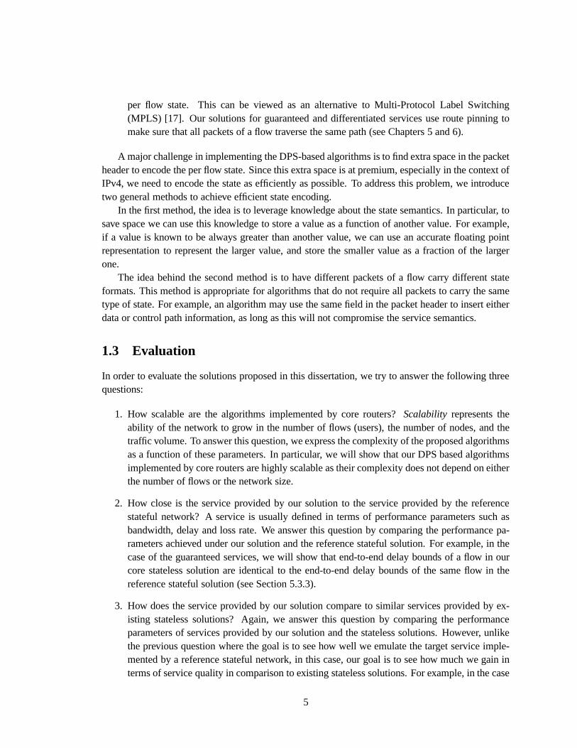
A major challenge in implementing the DPS-based algorithms is to find extra space in the packetheader to encode the per flow state. Since this extra space is at premium, especially in the context ofIPv4, we need to encode the state as efficiently as possible. To address this problem, we introducetwo general methods to achieve efficient state encoding.

In the first method, the idea is to leverage knowledge about the state semantics. In particular, tosave space we can use this knowledge to store a value as a function of another value. For example,if a value is known to be always greater than another value, we can use an accurate floating pointrepresentation to represent the larger value, and store the smaller value as a fraction of the largerone.

The idea behind the second method is to have different packets of a flow carry different stateformats. This method is appropriate for algorithms that do not require all packets to carry the sametype of state. For example, an algorithm may use the same field in the packet header to insert eitherdata or control path information, as long as this will not compromise the service semantics.

1.3 Evaluation

In order to evaluate the solutions proposed in this dissertation, we try to answer the following threequestions:

1. How scalable are the algorithms implemented by core routers? Scalability represents theability of the network to grow in the number of flows (users), the number of nodes, and thetraffic volume. To answer this question, we express the complexity of the proposed algorithmsas a function of these parameters. In particular, we will show that our DPS based algorithmsimplemented by core routers are highly scalable as their complexity does not depend on eitherthe number of flows or the network size.

2. How close is the service provided by our solution to the service provided by the referencestateful network? A service is usually defined in terms of performance parameters such asbandwidth, delay and loss rate. We answer this question by comparing the performance pa-rameters achieved under our solution and the reference stateful solution. For example, in thecase of the guaranteed services, we will show that end-to-end delay bounds of a flow in ourcore stateless solution are identical to the end-to-end delay bounds of the same flow in thereference stateful solution (see Section 5.3.3).

3. How does the service provided by our solution compare to similar services provided by ex-isting stateless solutions? Again, we answer this question by comparing the performanceparameters of services provided by our solution and the stateless solutions. However, unlikethe previous question where the goal is to see how well we emulate the target service imple-mented by a reference stateful network, in this case, our goal is to see how much we gain interms of service quality in comparison to existing stateless solutions. For example, in the case

5

of flow protection, we will show that none of the traditional solutions that exhibit the samecomplexity at core routers is effective in providing flow protection (see Section 4.4).

To address the above three questions, we use a mix of theoretical analysis, simulations, andexperimental results. In particular, to answer the first question, we use theoretical analysis to derivethe time and space complexity of the algorithms performed by both edge and core routers. To answerthe last two questions we derive worst-case or asymptotic bounds for the performance parametersthat characterize the service, such as delay and bandwidth. Whenever we cannot obtain such bounds,or if we want to relax the assumptions to fit more realistic scenarios, we rely on extensive simulationsby using an accurate packet level simulator such as ns-2 [78].

For illustration, consider our solution to provide per flow protection in a SCORE network (seeChapter 4). To answer the scalability question we show that in our solution a core router does notneed to maintain any per flow state, and that the time it takes to process a packet is independent ofthe number of flows that traverse the router, � . In contrast, with the existing solutions, each routerneeds to maintain state for every flow, and the time it takes to process a packet increases with

����� � .Consequently, our solution exhibits an ����� space and time complexity, as compared to existingsolutions that exhibit an � ����� space complexity, and an ��� ����� ��� time complexity. To answerthe second question we use theoretical analysis to show that the difference between the averagebandwidth allocated to a flow in a SCORE network and the bandwidth allocated to the same flowin the reference network is bounded. In addition, to answer the third question and to study morerealistic scenarios, we use extensive simulations.

Finally, to demonstrate the viability of our solutions and to explore the compatibility of the DPStechnique with IPv4, we present a detailed implementation in FreeBSD, as well as experimentalresults, to evaluate accuracy and implementation overhead.

1.4 Discussion

In this dissertation, we make two central assumptions. The first is that the ability to process packetson a per flow basis is beneficial, and perhaps even crucial, for supporting new emerging applicationsin the Internet. The second is that it is very hard, if not impossible, for traditional stateful solutionsto support these services in high-speed backbone routers. It is important to note that these two as-sumptions do not necessary imply that it is infeasible to support these emerging services in highspeed networks. They just illustrate the drawback of existing solutions that require routers to main-tain and manage per flow state. In this dissertation we eliminate this problem, by demonstrating thatit is possible to process packet on a per flow basis without requiring high-speed routers to maintainany per flow state.

The next two sections motivate these assumptions.

1.4.1 Why Per Flow Processing?

The ability to process packets on a per flow basis is important because it would allow us simul-taneously (1) to support applications with different performance requirements, and (2) to achievehigh resources utilization. To illustrate this point consider a simple example in which a file transfer

6

application and an audio application share the same link. On one hand, we want the file transferapplication to be able to use the entire link capacity, when the audio source does not send any traffic.On the other hand, when the audio application starts the transmission, we want this application to beable immediately to reclaim its share of the link capacity. In addition, since the audio application ismuch more sensitive to packet delay than the file transfer application, we should be able to preferen-tially treat the audio traffic in order to minimize its delay. As demonstrated by previous proposals,such a functionality can be easily provided in a stateful network in which routers process packets ona per flow basis [10, 48, 106].

A natural question to ask is whether performing packet processing at a coarser granularity, thatis, on a per class basis, wouldn’t allow us to achieve similar results. With such an approach, appli-cations with similar performance requirements would be aggregated in the same traffic class. Thiswould make routers much simpler to implement, as they need to differentiate between potentiallyonly a small number of classes, rather than a large number of flows. While this approach can go along way to support new applications in a scalable fashion, it has fundamental limitations. The mainproblem is that this approach implicitly assumes that all applications in the same class (1) cooperate,and (2) have similar requirements at each router. If assumption (1) does not hold, then malicioususers may arbitrarily degrade the service of other users in the same class. If assumption (2) doesnot hold, it is very hard to meet all application requirements and simultaneously achieve efficientresource utilization. Unfortunately, these assumptions do not necessarily hold in practice. As wediscuss in Chapter 4, cooperation is hard to achieve in today’s Internet: even in the absence of ma-licious users, there is a natural incentive for a user to aggressively send more and more traffic in thehope of making other users quit and grabbing their resources. Assumption (2) may not hold simplybecause applications care about the end-to-end performance, and not about the local performancethey experience at a particular router. As a result, applications with similar end-to-end performancerequirements may end up having very different performance requirements at individual routers. Forexample, consider two flows that carry voice traffic and belong to the same class, one traversinga 15 node path, and another traversing a three node path. In addition, assume that, as suggestedby recent studies in the area of interactive voice communication [7, 64], the tolerable end-to-enddelay for both flows is about 100 ms, and that the propagation delay alone along each path is 10ms. Then, while the first flow can afford a delay of only 6 ms per router, the second flow can afforda delay of up to 30 ms per router. But if both flows traverse the same router, the router will haveto provide a 6 ms delay to both flows, as it does not have any way to differentiate between the twoflows. Unfortunately, as we show in Appendix B.1, even under very low link utilization (e.g., 15%),it is very difficult to provide small delay bounds for all flows.

In summary, the ability to process packets on a per flow basis is highly desirable not only becauseit allows us to support applications with diverse needs, but also because it allows us to maximize theresource utilization by closely matching the application requirements to resource consumption.

1.4.2 Scalability Concerns with Stateful Network Architectures

In this section, we argue that the existing solutions that enable packet processing on a per flowbasis, that is, stateful solutions, have serious scalability limitations, and that these limitations makethe deployment of these solutions unlikely in the foreseeable future.

7

Recall that by scalability we mean the ability of a network to grow in the number of nodes, in thenumber of users it can support, and the traffic volume it can carry. Since in today’s Internet theseparameters increase at an exponential rate, scalability is a fundamental property of any protocolor algorithm to be deployed in the Internet. Indeed, according to recent statistics, Internet trafficdoubles every six months, and it is expected to do so until 2008 [88]. This growth is fueled byboth the exponential increase in the number of hosts, and the increase of bandwidth available toend users. The estimated number of hosts1 reached 72 million in February 2000, and it is expectedto reach 1 billion by 2008 [89]. In addition, the replacement of the ubiquitous 56 Kbps modemswith cable modems and Digital Subscriber Line (DSL) connections will increase home users’ accessbandwidth by at least one order of magnitude.

In spite of such a rapid growth, a question still remains: with the continuous increase in availableprocessor speed and memory capacity, wouldn’t it be feasible to implement stateful solutions at veryhigh speeds? In the remainder of this section, we answer this question. In particular, we first discusswhy it is hard to implement per flow solutions today, and then we argue that it will be even harderto implement them in the foreseeable future.

Very high-end routers today can switch on the order of terabits per second, and handle individuallinks of up to 20 Gbps [2]. With an average packet size of 500 bytes, an input has only 25 nsto process a packet. If we assume a 1 GHz processor that is capable of executing an instructionevery clock cycle, we have have just 25 instructions available per packet. During this time a routerhas to read the packet header, classify the packet to the flow it belongs to based on the fields inthe packet header, and then process the packet based on the state associated to the flow. Packetprocessing may include rate regulation, and packet scheduling based on some arbitrary parametersuch as the packet deadline. In addition, stateful solutions requires the set up of per flow state, andthe maintenance of this state consistency at all routers on the flow’s path. Maintaining the stateconsistency in a distributed network environment such as the Internet in which packets can be lostor arbitrary delayed, and routers can fail is a very difficult problem [4, 117]. Primarily due to thesetechnical difficulties, none of the high-end routers today implement stateful solutions.

While throwing more and more transistors at the problem will help, this will not necessarilysolve the problem. Even if, as Moore’s law predicts, processor performance continues to doubleevery 18 month, this increase may not be able to offset the faster increase of the Internet traffic vol-ume, which doubles every six moths. Worse yet, the increase in the router capacity not only reducesthe time available to process a packet, but can also increase the amount of work the router has todo per packet. This is because a higher speed router will handle more flows, and the complexityof some of the per packet operations, such as packet classifications, and scheduling, depends onthe number of flows. Even factoring out the algorithmic complexity, maintaining per flow state hasthe disadvantage of requiring a large memory footprint, which will negatively impact the memoryaccess times. Finally, the advances in semiconductor performances will do little to address the chal-lenge of maintaining the per flow state consistency, arguably the most difficult problem faced bytoday’s proposals to provide per flow services.

1This number represents only hosts with Domain Names. The actual number of computers that are connected to theInternet is much larger, but this number is much more difficult to estimate.

8

1.5 Organization

The rest of this dissertation is organized as follows: Chapter 2 provides background information.In the first part, it presents the IP network model which is the foundation of today’s Internet. Inthe second part, it discusses two of the most prominent proposals to provide better service in theInternet: Integrated Services and Differentiated Services. The chapter emphasizes the trade-offsbetween providing stronger semantics services and implementation complexity.

Chapter 3 describes the main components of our solution, and gives three simple examples toillustrate the DPS technique. The solution is then compared in terms of scalability and robustnessagainst traditional solutions aiming to provide similar services in the Internet.

Chapters 4, 5, and 6 describe three important network services that can be implemented byour solution: (1) flow protection to provide network support for congestion control, (2) guaranteedservices, and (3) service differentiation for large traffic aggregates, respectively. Our solution isthe first to implement flow protection for congestion control and guaranteed services in a statelesscore network architecture. We use simulations or experimental results to evaluate our solutions andcompare them to existing solutions that provide similar services.

Chapter 7 describes a novel approach called “verify-and-protect” to overcome some of the scal-ability and robustness limitations of our solution. We illustrate this approach in the context ofproviding per flow protection, by developing tests to accurately identify misbehaving nodes, andpresent simulation results to demonstrate the effectiveness of the approach.

Chapter 8 presents our prototype implementation which provides guaranteed services and perflow protection. It discusses compatibility issues with the IPv4 protocol, and the information encod-ing in the packet header. The latter part of the chapter discusses a light weight monitoring tool thatis able to continuously monitor the traffic on a per flow basis without affecting real-time guarantees.

Finally, Chapter 9 summarizes the conclusions of the dissertation, discusses the limitations ofour work, and ends with directions for future work.

9

10

Chapter 2

Background

Over the past decade, two classes of solutions have been proposed to provide better network ser-vices than the existing best effort service in the Internet: those maintaining the stateless propertyof the original Internet (e.g., Differentiated Services), and those requiring a new stateful architec-ture (e.g., Integrated Services). While stateful solutions can provide more powerful and flexibleservices such as per flow guaranteed services, and can achieve higher resource utilization, they areless scalable than stateless solutions. On the other hand, while stateless solutions are much morescalable, they offer weaker services. In this chapter, we first present all the mechanisms that a routerneeds to implement in order to support these solutions, and then discuss in detail the implementationcomplexity of each solution and the service quality it achieves.

The remainder of this chapter is organized as follows. Section 2.1 discusses the two main com-munication models proposed in the literature: circuit switching and packet switching. Section 2.2presents the Internet Protocol (IP) network model, the foundation of today’s Internet. In particular,the section discusses the operations performed by existing and the next generation routers on boththe data and control paths. Data path consists of all operations performed by a router on a packetas the packet is forwarded to its destination, and includes packet forwarding, packet scheduling,and buffer management. Control path consists of the operations and protocols used to initialize andmaintain the state required to implement the data path functionalities. Examples of control pathoperations are constructing and maintaining the routing tables, and performing admission control.Section 2.3 presents a taxonomy of services in a packet switching network. Based on this taxonomy,we discuss some of the most prominent services proposed in the context of the Internet: the besteffort service, flow protection, Integrated Services, and Differentiated Services. We then comparethese solutions in terms of the quality of service they provide and their complexity. Section 2.4concludes this chapter by summarizing our findings.

2.1 Circuit Switching vs. Packet Switching

Communication networks can be classified into two broad categories: packet switching and circuitswitching. Circuit switching networks are best represented by telephone networks, first developedmore than 100 years ago. In these networks, when two end points need to communicate, a dedicatedchannel (circuit) is set up between them. The channel remains open for the entire duration of thecall, no matter whether the channel is actually used or not.

11

Packet switching networks are best exemplified by the Asynchronous Transport Mode (ATM)and Internet Protocol (IP) networks. In these networks information is carried by packets. Eachpacket is switched and transmitted through the network based on the information contained in thepacket header. At the destination, the packets are reassembled to reconstruct the original informa-tion.

The most important advantage of packet switching over circuit switching is the ability to exploitstatistical multiplexing. Unlike circuit switching where no one can use an open channel if its end-points do not use it, with packet switching, active sources can use any excess capacity made availableby the inactive sources. In a networking environment with bursty traffic, allowing sources to sharenetwork resources can significantly increase network utilization. Indeed, a recent study shows thatthe ratio between the peak and the average rate is 3:1 for audio traffic, and as high as 15:1 for datatraffic [88].

The main drawback of packet switching networks is that statistical multiplexing can lead tocongestion. Network congestion happens when the arrival rate temporary exceeds the link capacity.In such a case, the network has to decide which traffic to drop, and which to transmit. In addition,end hosts are either expected to implement some form of congestion control, that is, to reduce theirsending rates when they detect congestion in the network, or to avoid congestion by making surethat they do not send more traffic than the available capacity of the network.

Due to its superior flexibility and resource usage, the majority of today’s networks are basedon packet switching technologies. The most prominent packet switching architectures are Asyn-chronous Transfer Mode [3, 12], and Internet Protocol (IP) [22]. ATM uses fixed size packets calledcells as the basic transmission unit, and was designed from the ground up to provide sophisticatedservices such as bandwidth and delay guarantees. In contrast, IP uses variable size packets, andsupports only one basic service: best effort packet delivery, which does not provide any timelinessor reliability guarantees. Despite the advantages of ATM in terms of quality of service, during thelast decade IP has emerged as the dominant architecture. For several technical and political reasonsthat try to explain this outcome see Tanenbaum [109].

As a result, our emphasis in this dissertation is on IP networks. While our SCORE/DPS tech-niques are applicable to packet switching networks in general, in this dissertation we examine themexclusively in the context of IP. In the remainder of this chapter, we first present the Internet Proto-col (IP) network model, which is the foundation of today’s Internet, and then we consider some ofthe major proposals to provide better services in the Internet, and discuss their trade-offs.

2.2 IP Network Model

The main service provided by today’s IP network is to deliver packets between any two nodes in thenetwork with a “reasonable” probability of success. The key component that enables this serviceis the router. Each router has two or more interfaces that attach it to multiple networks. Routersforward each packet based on the destination address in the packet’s header. For this purpose, eachrouter maintains a table, called routing table, that maps every IP address to an interface attachedto the router. Routing tables are constructed and maintained by the routing protocol. The routingprotocol is implemented by a distributed algorithm whose main function is to let routers learn thereachability of any host in the Internet along a “good” path. In general, the term of “good” applies

12

to the shortest1 path to a node. Thus, ideally, a packet travels along the shortest path from source todestination.

2.2.1 Router Architecture

As noted in the previous section, a router consists of a set of input interfaces at which packetsarrive, and a set of output interfaces, from which packets depart. The input and output interfaces areinterconnected by a high speed fabric that allows packets to be transfered from inputs to outputs.The main parameter that characterizes the fabric is the speedup. The speedup is defined as the ratiobetween (a) the maximum transfer rate across the fabric from an input to an output interface, and(b) the capacity of an input (output) link.

As a packet traverses a router, the packet can be stored at input, at output, or at both the inputand output interfaces. Based on where a router can store packets, routers are classified as inputqueueing, output queueing, or input-output queueing.

In an output-queueing router, when a packet arrives at the input, it is immediately transferredto the corresponding output. Since packets are enqueued and scheduled only at the outputs, thisarchitecture is easy to analyze and understand. For this reason, most analytical studies assume anoutput-queueing router model.

On the downside, the output-queueing router architecture requires a speedup as high as � , where� is the number of inputs. The worst case scenario occurs when all inputs simultaneously receivepackets for the same output. Since inputs are bufferless, the output has to be able to simultaneouslyreceive the � packets, hence the speedup of � . As the number of inputs in a modern router is quitelarge (e.g., it can exceed 32), building high-speed output-queueing routers is, in general, infeasible.That is why practically all of today’s routers employ some sort of input-output queueing. By beingable to buffer packets at the inputs, the speedup of the interconnection fabric can be significantlyreduced. However this comes at a cost: complexity. Since only the output has complete knowledgeof how packets are scheduled, complex distributed algorithms to control the packet transfer frominputs to outputs have to be implemented. Furthermore, this complexity makes the router behaviormuch more difficult to analyze.

In summary, while output-queueing routers are more tractable for analysis, the input and input-output queueing routers are more scalable and therefore easier to build. Fortunately, recent work hasshown that a large class of algorithms implemented by an output queueing router can be emulatedby an input-output queueing router which has an internal speedup of only 2 [21, 102]. Thus, atleast in principle, it is possible to build scalable input-output queueing routers that can emulate thebehavior of output queueing routers. For this reason, in the remainder of this dissertation, we willassume an output queueing router architecture.

Next, we discuss in more detail the output-queueing router architecture. Specifically, we presentall the operations that a router needs to perform on the data and control paths in order to implementcurrently proposed solutions that aim to provide better services than the best effort service, such asIntegrated Services and Differentiated Services.

1The most common metric used in today’s Internet is the number of routers (hops) on the path.

13

Classifier

Buffermanagement

Scheduler

flow 1

flow 2

flow n

output interface

router

input interface

output interface

Figure 2.1: The architecture of a router that provides per flow quality of service (QoS). Input interfaces userouting lookup or packet classification to select the appropriate output interface for each incoming packet,while output interfaces implement packet classification, buffer management, and packet scheduling. In to-day’s best effort routers, neither input nor output interfaces implement packet classification.

2.2.2 Data Path

Data path represents the set of operations performed by routers on a data packet as the packettravels from source to destination. The main functions performed by routers on the data path are:(1) routing lookup, (2) buffer management, and (3) packet scheduling. Routing lookup identifiesthe output interface where to forward each incoming packet, based on the destination address in thepacket’s header. Buffer management and scheduling are concerned with managing router resourcesin case of congestion. In particular, when the buffer overflows, or when it exceeds some predefinedthreshold, the router has to decide what packet to drop. Similarly, when there is more than onepacket in the buffer, the router has to decide what packet to transmit next. Usually, today’s routersimplement a simple drop-tail buffer management scheme, that is, when the buffer overflows, thepacket at the tail of the queue is dropped. Packets are scheduled on a First-In-First-Out (FIFO)basis.

However, currently proposed solutions to provide more sophisticated services than the best ef-fort service, such as per flow bandwidth and delay guarantees, require routers to perform a fourthfunction: (4) packet classification. Packet classification consists of mapping each incoming packetto the flow it belongs to. We use the term flow to denote a subset of packets that travel from onenode to another node in the network. Since both routing lookup and packet classification can beused to determine to which output interface a packet is forwarded, in the remainder of this sectionwe refer to both these operations as packet forwarding operations. Figure 2.1 depicts the relation-ship between the four functions in an output-queueing router that performs per flow management.In the remainder of this section, we present these functions in more detail. Since currently proposedsolutions to provide per flow service semantics require routers to maintain and manage per flowstate, we will elaborate on the complexity of these routers.

14

2.2.2.1 Packet Forwarding: Routing Lookup and Packet Classification

Packet forwarding is the main and the most complex function performed by today’s routers on thedata path. This function consists of forwarding each incoming packet to the corresponding outputinterface based on the fields in the packet header. Virtually all routers in today’s Internet forwardpackets based on their destination addresses. The process of finding the appropriate output portbased on the packet destination address is called routing lookup. However, to implement moresophisticated functionalities such as providing better services to selected customers or filtering outsome categories of traffic to enter the network, routers may need to use additional fields in the packetheaders to distinguish between different traffic classes. Examples of such fields are the sourceaddress to identify the incoming traffic of a selected customer, and the destination port number toidentify the traffic of different applications. The process of finding the class to which the packetbelongs to is called packet classification. Note that routing lookup is a particular case of packetclassification in which packets are classified based on one field: the destination address. In theremainder of this section we discuss in more detail routing lookup and packet classification.

Routing Lookup With routing lookup, each router maintains a table, called routing table, that mapseach IP address to an output interface. At the minimum, each entry in the routing table consists oftwo fields. The first field contains an address prefix, and the second field contains the identifier ofan output interface. The address prefix specifies the range of all IP addresses that share the sameprefix. Upon a packet arrival, the router searches its routing table for the longest prefix that matchesthe packet’s destination address, and then forwards the packet to the output interface specified bythe second field in the same entry. Thus, routing lookup consists of a search operation that retrievesthe longest prefix match.

To minimize the size of the routing table, IP addresses are assigned in blocks based on their pre-fixes [41]. As a result, the size of the largest routing tables today is about 70,000 entries [122], whichis three orders of magnitude smaller than the total number of hosts, which is about 72 million [89].

Traditional algorithms to implement the routing lookup are based on Patricia tries [72]. In thesimplest form, Patricia tries are binary trees in which each node represents a binary string thatencodes the path from the tree’s root to that node. As an example, consider such a tree in which allleft branches are labeled by 0, and all right branches are labeled by 1. Then, string 010 correspondsto the node that can be reached by walking down the tree from the root, first along the left branch,then along the right branch, and finally along the left branch. In the case of Patricia tries used toimplement routing lookup, each leaf node represents an address prefix. Since the height of the treeis bounded by the address size � , the worst case time complexity of the lookup operation is � ��� � .However, recent developments have significantly reduced this complexity. In particular, Waldvogelet al. [115] proposes a routing lookup algorithm that scales with the logarithm of the address size,while Degermark et al. [30] proposes a routing lookup algorithm tuned for IPv4 that takes less than100 instructions on an Alpha processor, and uses only up to eight memory references. Furthermore,by using a hardware implementation, Gupta et al. [50] proposes a pipelined architecture that canperform a routing lookup every memory cycle. However, these improvements do not come for free.The complexity of updating the routing table in these algorithms is much higher than in the caseof the algorithms based on Patricia tries. Nevertheless, this tradeoff is justified by the fact that, in

15

practice, updates are much less frequent than lookups.In summary, today it is possible to perform a routing lookup at the line speed, that is, without

slowing down a router that otherwise performs only packet queuing and dequeuing. Furthermore,this is expected to remain true in the foreseeable future. Even if the Internet continues to expand atits current rate, due to address aggregation, the routing tables are likely to remain relatively small.Assuming that the current ratio between the number of hosts and the size of the routing tables willnot change, and that, as predicted, the number of hosts will reach one billion by 2008 [88], weexpect that routing table size will increase by a factor of about 16 over the next eight years. Whilethis increase might seem considerable, it should be more than compensated for by the increase incomputer processing power and memory capacity. Indeed, according to Moore’s law, during thesame time span the semiconductor performances are expected to improve 40 times.

Packet Classification Current proposed solutions to provide Quality of Service (QoS) such asbandwidth and delay guarantees, require routers to maintain and manage per flow state. That is,upon a packet arrival, the router has to classify it to the class or flow the packet belongs to. Aclass is usually defined by a filter. A filter consists of a set of partially specified fields that define aregion in the packet space. Common fields used for packet classification are source and destinationIP addresses, source and destination port numbers, and the protocol type. An example of filter is������� � ��� ����� ����������� ����� ,

���� �

� �������� ����������� ����� ,

���� �� ����!�"� , ���#� �� ����!� 1000-1200,

���# ��$ �&%��(')�*� � , where � stands for “don’t care”. This filter represents the entire traffic goingfrom subnet 123.16.120.x to subnet 234.16.120.x with the destination port in the range1000-1200. As an example, the packet identified by �����#� � � � ���+��������������������� ,

���� �

����,�

��� ����������� ���-� ,���� �� ����!�.�� , ���#� �� ����/� 1080, ���# ��$ �$%��('0�2143 5 � belongs to this class, while

a packet sent by a host with the IP address �6�������-6�7���� does not. It is worth noting that routingis just a particular case of packet classification, in which each filter is specified by only one field:���� �

� �� .

It should come as no surprise that the classification problem is inherently difficult. Currentsolutions [51, 66, 96, 97] work well only for a relatively small number of classes, i.e., no more thanseveral thousand. This is because, as noted by Gupta and McKeown [51], the packet classificationproblem is similar to the point location problem in the domain of computation geometry. Givena point in an 8 dimensional space, this problem asks to find the enclosing region among a set ofregions. In the case of non-overlapping regions, the best bounds for � regions in an 8 dimensionalspace are ��� ����� ��� in time and � ���:9 � in space, or, alternatively, � � ����� 9<;>= ��� in time and ������� inspace. This suggests a clear trade-off between space and time complexities. It also suggests that it isvery hard to simultaneously achieve both speed and efficient memory usage. Worse yet, the packetclassification problem is even more difficult than the traditional point location problem as it allowsclass (region) overlapping.

2.2.2.2 Buffer Management

IP routers are based on a store-and-forward architecture, i.e., when a packet arrives at a router, thepacket is first stored in a buffer, and then forwarded. Since, in practice, buffers are finite, the routershave to cope with the possibility of packet loss. Even with infinite buffer capacity, there might be

16

the need to drop packets, as some congestion control schemes, such as TCP, rely on packet loss todetect network congestion.

Any buffer management scheme has to answer two questions: (1) when is a packet dropped?,and (2) which packet is dropped? In addition, per flow buffer management schemes have to answera third question: (3) which queue to drop from? Examples of policies that answer the first questionare: drop a packet when the buffer overflows (e.g., drop-tail), or when the average occupancy of thebuffer exceeds some threshold. Examples of policies that answer the second question are: drop thelast packet in the queue, the first packet in the queue, or a random packet. Finally, an example ofpolicy that answers the last question is to drop a packet from the longest queue.

While simple network services can be implemented by using a single queue which is sharedby all flows, solutions that provide more powerful services such as per flow bandwidth and delayguarantees require routers to maintain and manage a separate queue for each flow. In this case,the most expensive operation is usually to answer question (3), that is, to choose the queue to dropfrom. As an example, an algorithm that implements a policy that drops the packet from the longestqueue has ��� � ��� ��� complexity, where � is the number of non-empty queues. However, in practice,this complexity can be significantly reduced by grouping the queues that have the same size, or byapproximating the algorithm [108].

2.2.2.3 Packet Scheduling

The job of the packet scheduler is to decide what packet to transmit, if any, when the output linkbecomes idle. In routers that maintain per flow state this is accomplished in two steps: (1) select aflow that has a packet to send, and (2) transmit a packet from the flow’s queue.

Packet scheduling disciplines are classified into two broad categories: work conserving andnon-work conserving. In a work conserving discipline, the output link is busy as long as there isat least one packet in the system destined for that output. In contrast, in a non-work conservingdiscipline it is possible for an output link to be idle, despite the fact that there are packets in thesystem destined for that output. Virtually all routers in today’s Internet are work-conserving, andimplement a simple FIFO scheduling discipline. However, solutions to support better services thanbest effort, such as bandwidth and delay guarantees, require more sophisticated packet schedulingschemes. Examples of such schemes that are work conserving are: Static Priority [123], WeightedRound Robin [52], Virtual Clock [127], Weighted Fair Queueing [31], and Delay Earliest DeadlineDue [124]. Similarly, examples of non-work conserving disciplines are: Stop-and-Go [44], Jitter-Virtual Clock [126], Hierarchical Round Robin [63], and Rate Controlled Static Priority [123].

Many of the simpler disciplines such as FIFO, Static Priority, and Weighted Round Robin canbe easily implemented by constant time algorithms, i.e., algorithms that take ����� time to processeach packet. In contrast, the more sophisticated scheduling disciplines such as Virtual Clock andWeighted Fair Queueing are significantly more complex to implement. In general, the algorithmsto implement these disciplines associate with each flow a unique parameter that is used to selectthe flow to be served. Examples of such a parameter are the flow’s priority, and the deadline ofthe packet at the head of the queue. Flow selection is usually implemented by selecting the flowwith the largest or the smallest value. This can be accomplished by maintaining a priority queuedata structure in which the time complexity of selecting a flow is ��� � ��� ��� , where � represents the

17

number of flows in the queue.Non-work-conserving disciplines, as well as some of the more complex work-conserving dis-

ciplines, may employ a second parameter. The purpose of the second parameter is to determinewhether the flow with a non-empty queue is allowed to send or not. An example of such a param-eter is the eligible time. The packet at the head of the queue can be transmitted only if its eligibletime is smaller or equal to the system time. Obviously, the addition of a second parameter increasesthe implementation complexity. In many cases, the implementation is divided into two parts: arate controller that stores packets until they become eligible, and a scheduler that selects the flow’spacket to be transmitted based on the first parameter (e.g., deadline). Since the rate controller isusually implemented by constant time algorithms [10], the overall complexity of selecting a packetis generally dominated by the scheduling algorithm.

Once a flow is selected, one of its packets is transmitted – usually the packet at the head of thequeue – and the parameter(s) associated with the flow are eventually updated.

2.2.3 Control Path

The control path consists of all functions and operations performed by the network to set up andmaintain the state required by the data path. These functions are implemented by routing and sig-naling protocols.

2.2.3.1 Routing Protocol

The purpose of routing protocols is to set up and maintain routing tables of all routers in a network.Routing protocols are implemented by distributed algorithms that try to learn the reachability of anyhost in the network. In the Internet, routing protocols are organized in a two level hierarchy.

At the higher level, the Internet consists of a large number of interconnected autonomous sys-tems (ASs). An AS represents a distinct routing domain, which is usually administrated by a singleorganization such as a company or university. ASs are connected via gateways, which use inter-domain routing protocols to exchange routing information about which hosts are reachable by eachAS. As a result, each gateway constructs a routing table that maps each IP address to a neighbor ASthat knows a path to that IP address. The most common inter-domain routing protocol in use todayis Border Gateway Protocol (BGP) [86].

At the lower level within an AS, routers communicate with each other using an intra-domainrouting protocol. The purpose of these protocols is to enable routers to exchange locally obtainedinformation so that all routers within an AS have coherent and up to date information needed toreach any host within the AS. Examples of intra-domain routing protocols are Routing InformationProtocol (RIP) [54], and Open Shortest Path First (OSPF) [73].

The division of routing protocols into intra- and inter-domain is crucial for the scalability of theInternet. On one hand, this allows the deployment of sophisticated inter-routing protocols which cangather an accurate picture of the host reachability within an AS. On the other hand, the inter-domainrouting protocols present a much coarser information about host reachability. Unlike intra-domainrouting protocols that specify the path at the router granularity, these protocols specify the path atthe AS granularity. This tradeoff gives an organization maximum flexibility in managing its ownresources, without compromising routing scalability at the level of the entire Internet. Some key

18

factors affecting routing scalability, as well as some basic principles of designing scalable routingprotocols are presented by Yo [122].

In summary, as proved by the Internet’s own existence, the hierarchical routing architecture isboth scalable and robust. However, it should be noted that one of the main motivations behind thesedesirable properties is the weak semantic of the best effort service. The best effort service does notprovide any reliability or timeliness guarantees. As long as a “reasonable” number of packets reachtheir destinations, packet loss and packet reordering are acceptable. As a result, route changes,route oscillations, or even router failures do not necessary compromise the service. In contrast, withstronger service semantics such as the guaranteed service, existing routing protocols are not goodenough. The next section discusses these issues in more detail.

2.2.3.2 Signaling Protocol

To implement more sophisticated services such as per flow delay and bandwidth guarantees, weneed the ability to perform admission control and route pinning. The task of admission controlis to reserve enough resources on the path from source to destination in order to meet the servicerequirements. In turn, route pinning makes sure that all packets of the flow traverse the path onwhich resources have been reserved. Traditionally, these two functionalities are implemented bysignalling protocols such as Tenet Real-Time Channel Administration Protocol (RCAP) [8, 34], orRSVP [128]. The complexity of signaling protocols is primary due to the difficulty of maintainingthe state consistent in a distributed environment. In the remainder of this section we discus this issuein the context of both admission control and route pinning.

Admission Control Admission control makes sure that there are enough network resources onthe path from source to destination to meet the service requirements, such as delay and bandwidthguarantees. To better understand the issues with admission control consider the following exam-ple. Assume host A requests bandwidth reservation for a flow that has destination B. One possiblemethod to achieve this is to send a control message embedding the reservation request along the pathfrom A to B. Upon receiving this message, each router along the path checks whether it has enoughresources to accept the reservation. If it does, it allocates the required resources and then forwardsthe message. When host B receives this message, it sends back an acknowledgement to A. The reser-vation is considered successful if and only if all routers along the path have accepted it; otherwisethe reservation is rejected. While simple, this procedure does not account for various failures suchas packet loss and partial reservation failures. Partial reservation failures occur when only a subsetof routers along the path accept the reservation. In this case, the protocol has to undo the reservationat the routers that have accepted it. To handle packet loss, when a router receives a reservationrequest message, the router has to be able to tell whether it is a duplicate of a message already pro-cessed or not. To handle partial reservation failures, a router needs to remember the decision madefor the reservation request in a previous pass. For these reasons, all existing solutions maintain perflow reservation state, be it hard state as in ATM UNI [1], Tenet Real-Time Channel AdministrationProtocol (RCAP) [8, 34], or soft state as in RSVP [128]. However, maintaining consistent and dy-namic state in a distributed environment is in itself a challenging problem. Fundamentally, this isbecause admission control assumes a transaction-like semantic, which is very difficult to achieve in

19

a distributed system in the presence of message losses and arbitrary delays [4, 117].

Route Pinning Once a flow’s reservation request is accepted, the source can start sending datapackets. However, to meet the performance requirements negotiated during the admission control,we have to make sure that all packets of a flow traverse the same path. Otherwise, a packet cantraverse a path that does not have enough resources, which will lead to service violation. The oper-ation of binding a flow to a path (route) is called route pinning. Whenever the underlying routingprotocol does not support route pinning, this functionality can be provided by the signalling proto-cols together with the admission control. For example, in RSVP, when a node accepts a reservation,it also stores the next hop on the flow’s path in its database. Since these protocols maintain per flowstate, augmenting this state to store the next hop does not increase their complexity.

Alternatively, route pinning can be separated from admission control. One example is ATM [12]whose routing protocol natively supports route pinning. Another example is Multi-Protocol LabelSwitching (MPLS), recently proposed to perform traffic engineering in the Internet [17]. In bothATM and MPLS, the main idea is to perform routing based on identifiers that have local meaning,instead of identifiers that have global meaning such as IP addresses. Each router maintains a tablewhich maps each local identifier (label) to an output interface. Each packet carries a label thatspecifies how the packet is to be routed at the next hop. Before forwarding a packet, a routerreplaces the existing label with a new label that is used by the next hop to route the packet. Notethat this requires a router to also store the labels used by its neighbors. Besides route pinning, oneother major advantage of routing based on labels, instead of IP addresses, is performance. Insteadof searching for the longest prefix match, we only have to search for an exact match, which is muchfaster to implement.

On the downside, these routing schemes need a special protocol to distribute and maintain labelsconsistent. While in this case routers do not need to maintain per flow state, they still need tomaintain per path state. However, in practice, the number of paths that can traverse a core router canbe still quite large. In the worst case, this number increases with the square of the number of edgenodes. Thus, in the case of an AS that has hundreds of edge nodes, this number can be on the orderof hundred of thousands. Finally, label distribution protocols have to address the same challenges asother distributed algorithms that need to maintain state consistent in the presence of link and routerfailures, such as Tenet RCAP and RSVP.

2.2.4 Discussion

Among all the operations performed by routers on the data path, packet classification is arguablythe most complex. As discussed in Section 2.2.2.1, algorithms to solve this problem require at least��� � ��� ��� time and � ��� 9 � space, or, alternatively, at least � � ����� 9<;>= � time and � ����� space, where� represents the number of classes, and 8 represents the number of fields in a filter.

In contrast, most buffer management and packet scheduling algorithms have � ����� space com-plexity and ��� � ��� ��� time complexity. By trading resource utilization for speed, we can furtherreduce the time complexity to ��� ����� ����� ��� or even ����� . For example, [98] proposes an imple-mentation of Weighted Fair Queueing with ����� time complexity.

The important point to note here is that our DPS technique trivially eliminates the most complex

20

operation performed by core routers on the data path: packet classification. This is because, withDPS, the state required to process packets is carried by the packets themselves, instead of beingmaintained by core routers (see Section 1.1). Consequently core routers do not need to perform anypacket classification.

On the control path the most complex operation is arguably the admission control for whichcurrent solutions require routers to maintain per flow state. The main difficulty is to maintain theconsistency of the distributed state in the presence of packet losses, arbitrary packet delays, androuter failures.

Again, the main benefit of using DPS is that by eliminating the need for core routers to maintainper flow state, we trivially eliminate the need of maintaining this state consistent.

2.3 Network Service Taxonomy

In this section we present a general taxonomy of services in a packet switching network, and thenuse this taxonomy to describe the traditional best effort service, and the recently proposed servicesto enhance today’s Internet. We then describe and compare the existing solutions to implement theseservices.

The primary goal of a network is to provide services to its end-hosts. Services are usuallyclassified along two axes: (a) the granularity of the network abstraction to which the service applies,and (b) the “quality” of the service.

As the name suggests, packet switching networks are centered around the packet abstraction. Apacket represents the smallest piece of information that can be routed through the network. At ahigher level of granularity, we have the concept of a flow. A flow represents a subset of packets thattravel between two nodes in the network. If these nodes are routers, we will also use the terminologyof macro-flow. An example of a flow is the traffic of a TCP connection, while an example of a macro-flow is the traffic between two sub-networks. At an even higher level of abstraction, we have trafficaggregates over multiple destinations or sources. Examples of traffic aggregates are the entire webtraffic of a user, or the entire outgoing/incoming traffic of an organization.

Along the second axis, a service is described by a set of properties that can be either qualitativeor quantitative. Examples of qualitative properties are reliability and isolation. Isolation refers tothe ability of the network to protect the traffic of a flow against malicious sources that may floodthe network. Quantitative properties are described in terms of performance parameters such asbandwidth, delay, delay jitter and loss probability. Usually, these parameters are reported on anend-to-end basis. For example, the delay represents the total time it takes a packet to travel fromsource to its destination. Similarly, the delay jitter represents the maximum difference between themaximum and the minimum end-to-end delays experienced by any two packets of a flow. Note thatthe two quantitative and qualitative properties are not necessary orthogonal. For example, a servicethat guarantees a zero loss probability is trivially a reliable service.

Quantitative services can be further classified into absolute and relative services. Absoluteservices specify precise quantities that bound the service performance parameters such as worst casebandwidth or delay. In contrast, relative services specify the relative difference or ratio between theperformance parameters. Examples of absolute services are: “flow A is guaranteed a bandwidth of2 Mbps”, and “the loss probability of flow A is less than � ;�� ”. Examples of relative services are:

21

Service Network Abstraction Service DescriptionBest effort packet connectivity

Flow Protection flow protect well-behaved flowsagainst ill-behaved ones

Intserv Guaranteed flow bandwidth and delay guaranteesControlled-Load flow “weak” bandwidth guarantees

Diffserv Premium macro-flow bandwidth guaranteesAssured traffic aggregate over multiple “weak” bandwidth guarantees

destinations/sources

Table 2.1: A taxonomy of services in IP networks.

“flow A has twice the bandwidth of flow B”, and “flow A has a packet loss twice as small as flowB”.

Next, we discuss some of the most prominent services proposed in the context of the Internet:(1) the best effort service, (2) flow protection to provide network support for congestion control, (3)Integrated Services, and (4) Differentiated Services. Table 2.1 shows a taxonomy of these services.

2.3.1 Best Effort Service

Today’s Internet provides one simple service: the best effort service. This is fundamentally a con-nectivity service which allows any two hosts in the Internet to communicate by exchanging packets.As the name suggests, this service does not make any promise of whether a packet is actually de-livered to the destination, or whether the packets are delivered in order or not. Such a minimalistservice requires little support from routers. In general, routers just forward packets on a First-InFirst-Out (FIFO) basis. Thus, excepting the routing state, which is highly aggregated, a router doesnot need to maintain and manage any fine grained state about traffic. This simple architecture hasseveral desirable properties:

Scalability Since the only state maintained by routers is the routing state, today’s Internetarchitecture is highly scalable. In particular, address aggregation allows routers to maintainlittle state as compared to the number of hosts in the network. For example, a typical routertoday stores less than � ��� � � � entries [122] which is several orders of magnitude lower thanthe number of hosts in the Internet, which is around ��� million [89].

Robustness One of the most important goals in designing the Internet was robustness [22].In particular, the requirement was that two end-hosts should be able to communicate despiterouter and link failures, and/or network reconfiguration. The only case in which two hostscan no longer communicate is when the network between the two hosts is partitioned. Thefact that the state of a flow is maintained only by end-hosts and not by routers makes itsignificantly easier to ensure robustness, as router failures do not compromise the flow state.Had the flow state been kept by routers, complex algorithms to replicate and restore this statewould be needed to handle failures. Furthermore, such algorithms would be able to provide

22

protection against failures only if the number of routers failing is smaller than the number ofreplicas that failed.

There is one caveat with respect to the Internet robustness though. It can be argued that, toa large extent, today’s Internet is robust mainly because it provides a weak service semantic.Indeed, as long as the “majority” of packets still reach their destination, router or link failuresdo not compromise the service. In contrast, it is fundamentally more difficult to achieverobustness in the case of a strong semantic service such as the guaranteed service. In thiscase, a router or link failure can easily compromise the service. Note that even if back-uppaths were used to restore the service, time sensitive parameters such as delay may still beaffected during the recovery process.

Performance The simplicity of the router design allows efficient implementation at very highspeeds. Usually, these routers implement the FIFO scheduling discipline and drop-tail buffermanagement, which are both constant-time operations.

2.3.2 Flow Protection: Network Support for Congestion Control

Because of their reliance on statistical multiplexing, data networks such as the Internet must pro-vide mechanisms to control congestion. The current Internet relies on end-to-end congestion controlmechanisms in which senders reduce their transmission rates whenever they detect congestion in thenetwork. The most widely utilized form of congestion control is the additive-increase/multiplicative-decrease scheme implemented by TCP [57, 83], a scheme which has proven to be highly success-ful in preventing congestion collapse2 . However, the viability of this approach depends on onefundamental assumption: all end-hosts cooperate by implementing equivalent congestion controlalgorithms.

While this was a reasonable assumption when the Internet was primarily used by the researchcommunity, and the vast majority of traffic was TCP based, this is no longer true today. The emer-gence of new multimedia applications, such IP telephony, audio and video streaming, which usemore aggressive UDP based protocols, negatively affects the still predominant TCP traffic. Al-though there are considerable ongoing efforts to develop protocols for the new applications that areTCP friendly [6, 84, 85] – protocols that implement TCP like congestion control algorithms – theseefforts fail to address the fundamental problem: in an economic environment cooperation is notalways optimal. In particular, in case of congestion, the natural incentive of a sender is to send moretraffic in the hope that it will force other senders to back-off, and as a result it will be able to use theextra bandwidth. This incentive translates into a positive feed-back behavior, i.e., the more packetsthat are dropped in the network, the more packets the user sends, which can ultimately lead to con-gestion collapse. It is interesting to note that this problem resembles the “tragedies of commons”problem, well known in the economic literature [53].

Two approaches were proposed to address this problem: (1) flow identification and (2) fairbandwidth allocation. Both of these approaches require changes in the routers. In the followingsections, we discuss these approaches in more detail.

2Congestion collapse occurs when sources increase their sending rates when they experience losses, in the hope thatmore of their packets will get through. Eventually, this will lead to a further increase in the packet loss, and result inconsistent buffer overflow at the congested routers.

23

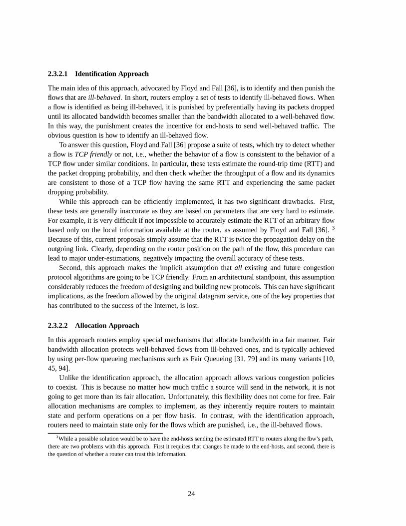
2.3.2.1 Identification Approach

The main idea of this approach, advocated by Floyd and Fall [36], is to identify and then punish theflows that are ill-behaved. In short, routers employ a set of tests to identify ill-behaved flows. Whena flow is identified as being ill-behaved, it is punished by preferentially having its packets droppeduntil its allocated bandwidth becomes smaller than the bandwidth allocated to a well-behaved flow.In this way, the punishment creates the incentive for end-hosts to send well-behaved traffic. Theobvious question is how to identify an ill-behaved flow.

To answer this question, Floyd and Fall [36] propose a suite of tests, which try to detect whethera flow is TCP friendly or not, i.e., whether the behavior of a flow is consistent to the behavior of aTCP flow under similar conditions. In particular, these tests estimate the round-trip time (RTT) andthe packet dropping probability, and then check whether the throughput of a flow and its dynamicsare consistent to those of a TCP flow having the same RTT and experiencing the same packetdropping probability.

While this approach can be efficiently implemented, it has two significant drawbacks. First,these tests are generally inaccurate as they are based on parameters that are very hard to estimate.For example, it is very difficult if not impossible to accurately estimate the RTT of an arbitrary flowbased only on the local information available at the router, as assumed by Floyd and Fall [36]. 3

Because of this, current proposals simply assume that the RTT is twice the propagation delay on theoutgoing link. Clearly, depending on the router position on the path of the flow, this procedure canlead to major under-estimations, negatively impacting the overall accuracy of these tests.

Second, this approach makes the implicit assumption that all existing and future congestionprotocol algorithms are going to be TCP friendly. From an architectural standpoint, this assumptionconsiderably reduces the freedom of designing and building new protocols. This can have significantimplications, as the freedom allowed by the original datagram service, one of the key properties thathas contributed to the success of the Internet, is lost.

2.3.2.2 Allocation Approach

In this approach routers employ special mechanisms that allocate bandwidth in a fair manner. Fairbandwidth allocation protects well-behaved flows from ill-behaved ones, and is typically achievedby using per-flow queueing mechanisms such as Fair Queueing [31, 79] and its many variants [10,45, 94].

Unlike the identification approach, the allocation approach allows various congestion policiesto coexist. This is because no matter how much traffic a source will send in the network, it is notgoing to get more than its fair allocation. Unfortunately, this flexibility does not come for free. Fairallocation mechanisms are complex to implement, as they inherently require routers to maintainstate and perform operations on a per flow basis. In contrast, with the identification approach,routers need to maintain state only for the flows which are punished, i.e., the ill-behaved flows.

3While a possible solution would be to have the end-hosts sending the estimated RTT to routers along the flow’s path,there are two problems with this approach. First it requires that changes be made to the end-hosts, and second, there isthe question of whether a router can trust this information.

24

2.3.3 Integrated Services

As new applications such as IP telephony, video-conferencing, audio and video streaming, and dis-tributed games are deployed in the Internet, services more sophisticated than best effort are needed.Unlike previous applications such as file transfer, these new applications have much stricter timeli-ness and bandwidth requirements. For example, to enable natural interaction, the end-to-end delayneeds to be below human perception. Previous studies concluded that for natural hearing this delayshould be around 100 ms [64]. Since in a global network the propagation delay alone is about 100ms, meeting such tight delay requirements is a very challenging task [7].

To support these new applications, IETF has proposed a new service model called IntegratedServices or Intserv [82]. Intserv uses flow abstraction. Two services were defined within the Intservframework: Guaranteed and Controlled-Load services.

2.3.3.1 Guaranteed Service

Guaranteed service is the strongest semantic service proposed in the context of the Internet sofar [93]. Guaranteed service has the ability to provide per flow bandwidth and delay guarantees.In particular, a flow can be guaranteed a minimum bandwidth, and, given the arrival process ofthe flow, a maximum end-to-end delay. This way, Guaranteed service provides ideal support forreal-time applications such as IP telephony.

However, this comes at the cost of a significant increase in complexity: current solutions requirerouters to maintain and manage per flow state on both data and control paths. On the data path, arouter has to perform per flow classification, buffer management and scheduling. On the controlpath, routers have to maintain per flow forwarding state and perform per flow admission control.During the admission control, each router on the flow’s path reserves network resources, such as thelink capacity and buffer space, to make sure that the flow’s bandwidth and delay requirements aremet.

2.3.3.2 Controlled-Load Service

For applications that do not require strict service guarantees, IETF has proposed a weaker se-mantic service within the Intserv framework: the Controlled-Load service. As defined by Wro-clawski [121], the Controlled-Load service “tightly approximates the behavior visible to applica-tions receiving best effort service *under unloaded conditions* from the same series of networkelements”. More precisely, the Controlled-Load service ensures that (1) the packet loss is not sig-nificantly larger than the basic error rate of the transmission medium, and (2) the end-to-end delayexperienced by a very large percentage of packets does not greatly exceed the end-to-end propaga-tion delay. The Controlled-Load service is intended to provide better support for a broad class ofapplications that have been developed for use in today’s Internet. Among the applications that fallinto this class are the “adaptive and real-time applications” such as video and audio streaming.

While the Controlled-Load service still requires routers to perform per flow admission controlon the control path, and packet classification, buffer management, and scheduling on the data path,some of these operations can be significantly simplified. For example, the scheduling can be imple-mented by a simply weighted round robin discipline, which has � ��� time complexity. Thus, the

25

Controlled-Load trades a lower quality of service for a simpler implementation.In summary, although Intserv provides much more powerful and flexible services than today’s

Internet – services that would answer the needs of the new emerging applications – concerns withrespect to its complexity and scalability have hampered its adoption. In fact, except in small test-beds, Intserv solutions have yet to be deployed.

2.3.4 Differentiated Services

To alleviate the scalability problems that have plagued Intserv, recently a new service model, calledDifferentiated Services (Diffserv), has been proposed [13, 75]. The Diffserv architecture differen-tiates between edge and core routers. Edge routers maintain per flow or per aggregate state. Corerouters maintain state only for a very small number of traffic classes; they do not maintain any finegrained state about the traffic. Each packet carries in its header a six bit field, called the Differ-entiated Service (DS) field, which specifies the class to which the packet belongs. The DS fieldis initialized by the ingress router upon the packet arrival. In turn, core routers use the DS fieldto classify and process the packets. Since the number of classes at a core router is very small,packet processing can be very efficiently implemented. This makes the Diffserv architecture highlyscalable.

Two services were proposed in the context of the Diffserv architecture: Assured and Premiumservices.

2.3.4.1 Assured Service

The Assured service [24, 55] is a large granularity service, that is, the service is associated withthe aggregate traffic of a customer from/to multiple hosts. The service contract between a customerand the Diffserv network or ISP is called the service profile. A service profile is usually defined interms of absolute bandwidth and relative loss. As an example, an ISP can provide two service levels(classes): silver and gold, where the gold service has the lowest loss probability. A possible serviceprofile would offer transmission of 10 Mbps of customer’s web traffic by using the silver service.

In the Assured service model, ingress routers perform three functions. They (a) monitor theaggregate traffic from each user to make sure that no user exceeds its traffic profile, (b) downgradethe user’s traffic to a lower service level if the user exceeds its profile, and (c) initialize the DS fieldin the packet headers with the code-point associated to the service. Thus, ingress routers need tokeep state for each profile or user. In contrast, core routers do not need to keep such state, as theirfunction reduces to process the packets based on the code-points carried by the packets.

While the fixed bandwidth profile makes the Assured service very compelling, it also makes itvery challenging to implement. This is due to a fundamental conflict between maximizing resourceutilization and achieving high service assurance. Since a service profile does not specify how thetraffic is distributed through the network, the network has to make conservative assumptions toachieve high service assurance. At the limit, to guarantee zero loss, the network has to assume thatthe entire assured traffic traverses the slowest link in the network! Clearly, such an assumption leadsto a very low resource utilization, which can be unacceptable.

An alternate approach is to define service profiles in relative rather than absolute terms. Such anexample is the User-Share Differentiation (USD) approach [116]. With USD each user is assigned

26

a share (weight) that specifies the relative fraction of the capacity that a user is entitled to receiveon each link in the network. This is equivalent to a network in which the capacity of each linkis allocated by a Weighted Fair Queueing algorithm. The problem with such an approach is thatthe core routers need to maintain per user state, which can negate the scalability advantage of theDiffserv architecture. In addition, with USD, there is little correlation between the share of a userand the aggregate throughput it will receive. For example, two users that are assigned the same sharecan see drastically different aggregate throughputs. A user that has traffic for many destinations(thus traverse many different paths) can potentially receive much higher aggregate throughput thana user that has traffic for only a few destinations.

2.3.4.2 Premium Service

Unlike the Assured service which can be associated with an aggregated traffic to/from multiplehosts, Premium service provides the equivalent of a dedicated link of fixed bandwidth between twoedge routers [60]. To implement this service, the network has to perform admission control. Thecurrent proposals assume a centralized architecture: each domain is associated with a database,called Bandwidth Broker (BB), that has complete knowledge about the entire domain. To set up aflow across a domain, the domain’s BB checks first whether there are enough resources between thetwo end points of the flow across the domain. If yes, the request is granted and the BB’s database isupdated accordingly.

On the data-path, ingress routers perform two functions. They (a) shape the traffic associatedto a service profile, that is, make sure that the traffic does not exceed the profile by delaying theexcess packets4 , and (b) insert the Premium service code-point in the DS-files. In turn, core routersforward the premium traffic with high priority.

As a result, the Premium service can provide effective support for real-time traffic. A naturalquestion to ask is what is the difference between the Premium service and the Guaranteed serviceproposed by Intserv. Though at the surface they are quite similar, there are two important differencesbetween them.

First, while the Guaranteed service can provide both per flow bandwidth and delay differentia-tion, the Premium service can provide only per flow bandwidth differentiation. This is because corerouters do not differentiate between premium packets on a per flow basis – all premium packets aresimply processed in a FIFO order. Thus, the only possibility to meet different delay requirementsfor different flows is to guarantee the smallest delay required by any flow to all flows. Unfortunately,this can result in very low resource utilization for the premium traffic. In particular, as shown byStoica and Zhang [105], even if the fraction that can be allocated to premium traffic on every link inthe network is very low (e.g., 10%), the worst case queueing delay across a large network (e.g., 15routers) can be relatively large (e.g., 240 ms). In contrast, Intserv can achieve both higher resourceutilization and tighter delay bounds, by better matching flow requirements to resource usage.

Second, the centralized bandwidth broker architecture proposed to perform admission controlin the case of the Premium service is adequate only for coarse grained flows that are active overlong time scales. In contrast, because the Guaranteed service uses a distributed admission control

4Note that this is different from the Assured service, where the excess traffic is let into the network, but its priority isdowngraded.

27

architecture, it can support fine grained reservations over small time scales.The price paid by the Guaranteed service is again complexity. Unlike the Premium service, the

Guaranteed service requires routers to maintain per flow state on both the data and the control paths.

2.4 Summary

In the first part of this chapter, we have discussed the IP network model. In particular we havepresented the router architecture and discussed the implementation complexities of both the dataand control paths.

In the second part of this chapter, we have presented the best-known proposals to improve thebest effort service in today’s Internet: (a) flow protection to provide effective support for congestioncontrol, (b) Integrated Services (Intserv) model, and (c) Differentiated Services (Diffserv) model.Of all these models, only Diffserv admits a known scalable implementation, as core routers arenot required to maintain any per flow state. However, to achieve this, Diffserv makes significantcompromises. In particular, the Assured service cannot achieve simultaneously high service assur-ance and high resource utilization. Similarly, the Premium service cannot provide per flow delaydifferentiation, and it is not adequate for fine grained and short term reservations.

In this dissertation we address these shortcomings by developing a novel solution that can im-plement all of the above per flow services (i.e., flow protection, guaranteed and controlled-loadservices) in the Internet without compromising its scalability. In the next chapter, we present anoverview of our solution.

28

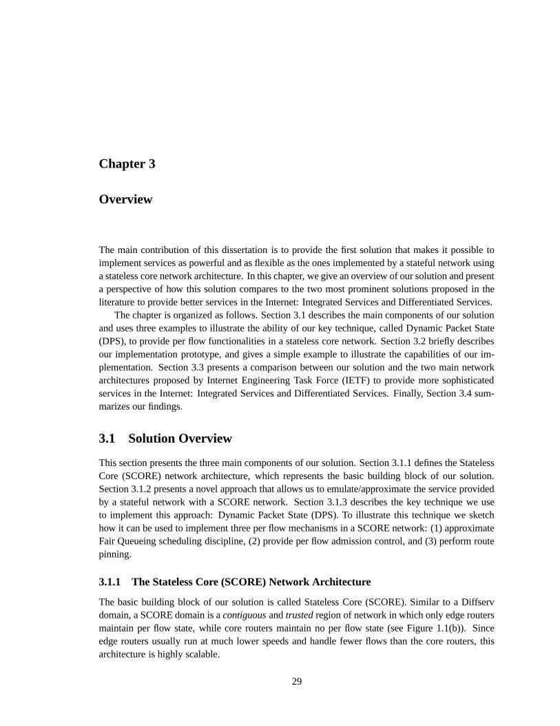
Chapter 3

Overview

The main contribution of this dissertation is to provide the first solution that makes it possible toimplement services as powerful and as flexible as the ones implemented by a stateful network usinga stateless core network architecture. In this chapter, we give an overview of our solution and presenta perspective of how this solution compares to the two most prominent solutions proposed in theliterature to provide better services in the Internet: Integrated Services and Differentiated Services.

The chapter is organized as follows. Section 3.1 describes the main components of our solutionand uses three examples to illustrate the ability of our key technique, called Dynamic Packet State(DPS), to provide per flow functionalities in a stateless core network. Section 3.2 briefly describesour implementation prototype, and gives a simple example to illustrate the capabilities of our im-plementation. Section 3.3 presents a comparison between our solution and the two main networkarchitectures proposed by Internet Engineering Task Force (IETF) to provide more sophisticatedservices in the Internet: Integrated Services and Differentiated Services. Finally, Section 3.4 sum-marizes our findings.

3.1 Solution Overview

This section presents the three main components of our solution. Section 3.1.1 defines the StatelessCore (SCORE) network architecture, which represents the basic building block of our solution.Section 3.1.2 presents a novel approach that allows us to emulate/approximate the service providedby a stateful network with a SCORE network. Section 3.1.3 describes the key technique we useto implement this approach: Dynamic Packet State (DPS). To illustrate this technique we sketchhow it can be used to implement three per flow mechanisms in a SCORE network: (1) approximateFair Queueing scheduling discipline, (2) provide per flow admission control, and (3) perform routepinning.

3.1.1 The Stateless Core (SCORE) Network Architecture

The basic building block of our solution is called Stateless Core (SCORE). Similar to a Diffservdomain, a SCORE domain is a contiguous and trusted region of network in which only edge routersmaintain per flow state, while core routers maintain no per flow state (see Figure 1.1(b)). Sinceedge routers usually run at much lower speeds and handle fewer flows than the core routers, thisarchitecture is highly scalable.

29

3.1.2 The “State-Elimination” Approach

Our ultimate goal is to provide better services in today’s Internet without compromising its scalabil-ity and robustness. To achieve this goal, we propose a two step approach, called “State-Elimination”approach (see Figure 1.1). In the first step we define a reference stateful network that provides thedesired service. In the second step, we try to approximate or, if possible, to emulate the serviceprovided by the reference stateful network in a SCORE network. In this way we are able to pro-vide services as powerful and as flexible as the ones implemented by stateful networks in a mostlystateless network, i.e., in a SCORE network. In Chapters 4, 5 and 6, we illustrate this approachby considering three of the most important services proposed to enhance today’s Internet: flowprotection, guaranteed services, and relative service differentiation.

We note that similar approaches have been proposed in the literature to approximate the func-tionality of an idealized router that implements a bit-by-bit round-robin scheduling discipline witha stateful router that forwards traffic on a per packet basis [10, 31, 45, 79]. However, our approachdiffers from these approaches in two significant aspects. First, the state-elimination approach is con-cerned with emulating the functionality of an entire network, rather than of a single router. Second,unlike previous approaches that aim to approximate an idealized system with a stateful system, ourgoal is to approximate the functionality of a stateful system with a stateless core system.

3.1.3 The Dynamic Packet State (DPS) Technique

DPS is the key technique that allows us to implement the above services in a SCORE network. Themain idea behind DPS is very simple: instead of having routers install and maintain per flow state,have packets carry the per flow state. This state is inserted by ingress routers, which maintain perflow state. In turn, a core router processes each incoming packet based on (1) the state carried inthe packet’s header, and (2) the router’s internal state. Before forwarding the packet to the next hop,the core router updates both its internal state and the state in the packet’s header (see Figure 1.2).By using DPS to coordinate actions of edge and core routers along the path traversed by a flow,distributed algorithms can be designed to approximate the behavior of a broad class of statefulnetworks using networks in which core routers do not maintain per flow state.

To give an intuition of how the DPS technique is working, next we present three examples: (1)approximates the Fair Queueing algorithm, (2) estimates the aggregate reservation for admissioncontrol purposes, and (3) binds a flow to a particular path (i.e., perform route-pinning).

3.1.3.1 Example 1: Fair Bandwidth Allocation

Flow protection is one of the most desirable enhancements of today’s best effort service. Flow pro-tection allows diverse end-to-end congestion control schemes to seamlessly coexist in the Internet,and protect well behaved traffic against malicious or ill behaved traffic. The solution of choice toachieve flow protection is to have routers implement fair bandwidth allocation [31]. In an idealizedsystem in which a router can provide services at the bit granularity, fair bandwidth allocation can beachieved by using a bit-by-bit round robin discipline.

For clarity, consider three flows with the arrival rates of 8, 6, and 2 bits per second (bps),respectively, that share a 10 bps link. Assume that the traffic of each flow arrives one bit at a time,

30

flow 1

flow 2

flow 3

8 8 8 8

666

2

………

flow 1

flow 2

flow 3

edge node

core node

4 4

4

2

4

Figure 3.1: Example illustrating the CSFQ algorithm at a core router. An output link with a capacity of10 is shared by three flows with arrival rates of 8, 6, and 2, respectively. The fair rate of the output link inthis case is ��� �

. Each arrival packet carries in its header the rate of the flow it belongs to. According toEq. (3.3) the dropping probability for flow 1 is 0.5, while for flow 2 it is 0.33. Dropped packets are indicatedby crosses. Before forwarding a packet, its header is updated to reflect the change in the flow’s rate due topacket dropping (see the packets at the right-hand side of the router).

and it is periodic with period ���� , where � is the flow rate. Thus, during one second, exactly 16bits are received, and exactly 10 bits can be transmitted. During each round, the scheduler transmitsexactly one bit form every flow that has a packet to send. Since in the worst case, flow 3 is visitedonce every ��� � sec, and it has an arrival rate of only one bit every

� ��� sec, it follows that all ofits traffic is served. This leaves the other two flows to share the rest of 8 bps of the link capacity.Since arrival rates of both flows 1 and 2 are larger than half of the remaining capacity, each flow willreceive half of it, i.e., 4 bps. As a result, under the bit-by-bit round robin discipline, the three flowsare allocated bandwidth of 4, 4, and 2 bps, respectively. The maximum rate allocated to a flow on acongestion link is called fair rate. In this example the fair rate is 4.

In general, given � flows that traverse a congested link of capacity, � , the fair rate � is definedsuch that �

� =�� �� � �

� � � ��� � (3.1)

where �

represents the arrival rate of flow � . By applying this formula to the previous example, we

have �� �� ��� � � ��� �� �� ��� � � ��� �� �� � � � � � � � , which gives us � ��� . If the link is not congested,that is, if �

�� = �

��� , the fair rate, � , is by convention defined as being the maximum among all

arrival rates.Thus, with the bib-by-bit round robin, the service rate allocated to a flow, � , with the arrival rate,

�

, is

�� �� � �� � � � (3.2)

31

The first algorithm to approximate the bit-by-bit round robin in a packet system was proposedby Demers et al. [31], and it is called Fair Queueing. Eq. (3.2) directly illustrates the protectionproperty of Fair Queueing, that is, a flow with enough demand is guaranteed to receive its fair rate� , irrespective of the behavior of the other flows. To put it in another way, a flow cannot deny serviceto other flows because no matter how much and what type of traffic it pumps into the network, itwill not get more than � on the congested link.

While fair queueing can fully provide flow protection, it is more complex to implement than tra-ditional FIFO queueing with drop-tail, which is the most widely implemented and deployed mech-anism in routers today. For each packet that arrives at the router, the routers needs to classify thepacket into a flow, update per flow state variables, and perform per flow scheduling.

Our goal is to eliminate this complexity from the network core by using a SCORE networkarchitecture to approximate the functionality of a reference network in which every router performsFair Queueing. In the following sections, we describe a DPS based algorithm, called Core-StatelessFair Queueing (CSFQ) that achieves this goal.

The key idea of CSFQ is to have each packet carry the rate estimate of the flow it belongs to.Let �� denote the rate estimate carried by a packet of flow � . The rate estimate is computed by edgerouters and then inserted in the packet header. Upon receiving the packet, a core router forwards itwith the probability

��� �� �� � � � �� �� �

(3.3)

and drops it with the probability ���� .It is easy to see that by forwarding each packet with the probability � , the router effectively

allocates to flow, � , a rate �

��� � �� �� ���� � � � , which is exactly the rate the flow would receive

under Fair Queueing (see Eq. (3.2)). If �

� , the router also updates the packet label to � . This is

to reflect the fact that when the flow’s arrival rate is larger than � , the flow’s rate after traversing thelink drops to � (see Figure 3.1).

It is also easy to see that with CSFQ core routers do not require any per flow state. Upon packetarrival, a core router needs to compute only the dropping probability, � , which depends exclusivelyon the estimated rate carried by the packet, and the fair rate � that is locally computed by the router.(In Chapter 4, we show that computing � does not require per flow state either.)

Figure 3.1 shows an example in which three flows with incoming rates of 8, 6, and 2, respec-tively, share a link of capacity 10. Without going into details, we note that in this case � ��� . Then,from Eq. (3.3), it follows that the forwarding probabilities of the three flows are 0.5, 0.66, and 1,respectively. As a result, on the average, one out of two packets of flow 1, one out of three packetsof flow 2, and no packets of flow 3, are dropped. Note that before forwarding the packets of flows 1and 2, the router updates the rate estimates in their headers to � . This is to reflect the change of theflow rates as a result of packet dropping.

3.1.3.2 Example 2: Per Flow Admission Control

In this example we consider the problem of performing per flow admission control. The role ofthe admission control is to check whether there are enough resources on the data path to grant areservation request. For simplicity, we assume that admission control is limited to bandwidth. When

32

flow 1

flow 2

20 15…flow 1 (rsv1 = 5)

edge node

core node

10234

6 86433…

T =10

flow 2 (rsv2 = 2)

…

…

Figure 3.2: Example illustrating the estimation of the aggregate reservation. Two flows with reservationsof 5, and 2, respectively, share a common link. Ingress routers initialize the header of each packet accordingto Eq. (3.4). The aggregate reservation is estimated as the ratio between the sum of the values carried inthe packets’ headers during an averaging time interval of length � . In this case the estimated reservation is����� ����� � � .

a new flow makes a reservation request, each router on the path from source to destination checkswhether it has enough bandwidth to accommodate the new flow. If all routers can accommodate theflow, then the reservation is granted.

It is easy to see that to decide whether a new reservation request � ��� can be accepted or not,a router needs only to know the current aggregate reservation,

�, on the output link, that is, how

much bandwidth it has reserved so far. In particular, if the capacity of the output link is � , then therouter can accept a reservation, � ��� , as long as � ��� � ��� � . Unfortunately, it turns out that main-taining the aggregate reservation,

�, in the presence of packet loss and partial reservation failures

is not trivial. Intuitively, this is because the admission control needs to implement transaction-likesemantics. A reservation is granted if and only if all routers along the path accept the reservation. Ifa router cannot accept a reservation, then all routers that have accepted the reservation have to rollback to the previous state, so they need to remember that state. Similarly, if a reservation requestmessage is lost, and the request is resent, then a router has to remember whether it has receivedthe original request, and if yes, whether the request was granted or denied. For all these reasons,the current proposed solutions for admission control such as RSVP [128] and ATM UNI [1] requirerouters to maintain per flow state.

In the remainder of this section we show that by using DPS it is possible to perform admissioncontrol in a SCORE network, that is, without core routers maintaining any per flow state.

At the basis of our scheme lies a simple observation: if all flows were sending at their reservedrates, then it is trivial to maintain the aggregate reservation

�; each router only needs to measure

the rate of the aggregate traffic. Consider the example in Figure 3.2, and assume that flow 1 hasa reservation of 5 Kbps, and flow 2 has a reservation of 2 Kbps. If the two flows were sendingexactly at their reserved rates, i.e., flow 1 at 5 Kbps, and flow 2 at 2 Kbps, the hi-lighted router (see

33

Figure 3.2) can simply estimate the aggregate reservation of 7 Kbps, by measuring the rate of theaggregate arrival traffic.

The obvious problem with the above scheme is that most of the time flows do not send at theirreserved rates. To address this problem, we associate a virtual length to each packet. The virtuallength is such that if the lengths of all packets of a flow where equal to their virtual lengths, then theflow sends at its reserved rate. More precisely, the virtual length of a packet represents the amount oftraffic that the flow was entitled to send according to its reserved rate since the previous packet hasbeen transmitted. Let � ���

denote the reservation of flow � , and let ���

and ��� � =

denote the departure

times of the � -th and ��� � �� -th packets of flow � . Then the ��� � �� -th packet will carry in its headera virtual length

��� � � =

� � ���

�� � � � = � � � � � (3.4)

The virtual length of the first packet of the flow is simply the actual length of the packet. Thevirtual length is computed and inserted in the packet header by the ingress router upon the packetdeparture. In turn, core routers use the packet virtual lengths to estimate the aggregate reservation.For illustration, consider again the example in Figure 3.2, where flow 1 has a reservation � ��� = of �Kbps. For the purpose of this example, we neglect the delay jitter, and assume that no packets aredropped inside the core. Suppose the inter-arrival times of the first four packets of flow 1 are 2 sec,3 sec, and 4 sec, respectively. Since in this case the packet inter-arrival times at core routers areequal to the packet inter-departure times at the ingress, according to Eq. (3.3), the 2nd, 3rd, and 4thpacket of flow 1 will carry in their headers ����� = � � ��� =

�� � � Kb, ���� = � � ��� =

�� � � Kb, and

���� = � � ��� =

�� � � � Kb, respectively.

Next, note that the sum of the virtual lengths, ��� � , of all packets of flow � that arrive at a core

router during an interval of length , provides a fair approximation of the amount of traffic that theflow is entitled to send during time at its reserved rate. Then, the reserved bandwidth of flow � ,can be estimated as �

�� �

�� � � (3.5)

By extrapolation, a core router can estimate the aggregate reservation�

on the outgoing linkby simply computing � �� � �� , where � �� � represents the sum of the virtual lengths of all packetsthat arrive during an interval of length . Finally, it is worth noting that to perform this computationcore routers do not need to maintain any per flow state – they just need to maintain a global variable,� �� � , that is updated every time a new packet arrives.

In the example shown in Figure 3.2, assume an averaging interval � � sec (represented bythe shaded area). Then we have � �� � ��� = �� ����� � � � � � � � Kb, which gives us an estimate ofthe aggregate reservation of �� ��� �� � �� .� � ��� Kbps, which is “reasonably” close to the actualaggregate reservation

� � � Kbps.In Chapter 5 we derive an upper bound of the aggregate reservation along a link, instead of just

an estimate. By using the upper bound we can guarantee that the link is never over-provisioned.

3.1.3.3 Example 3: Route pinning

Many applications such as traffic engineering and guaranteed services require that all packets ofa flow to follow the same path. To achieve this goal, many solutions such as Tenet RCAP [8]

34

path label port #… …

1000 11010 2… …

routing table

0100 1100 � � 1000

0110 1100 � � 1010

0100 1100 � � 1000

port #1

port #2

flow 1

flow 2

flow 3

………

flow 1 (0100 = 1100 1011 0011)

edge node

core node0001

1011

1100

1001

0011

01001000

0010

flow 2 (0100 = 1100 1011 0011)

flow 3 (1010 = 1100 1001 0011)

1000

1000

0011

to 1011

to 1001

0100

0100

1010

1100

Figure 3.3: Example illustrating the route pinning algorithm. Each packet contains in its header the path’slabel, defined as the xor over the identifiers of all routers on the remaining path to the egress. Upon packetarrival, the packet’s header is updated to the label of the remaining path. The routing decisions are exclusivelybased on the packet’s label (here the labels are assumed to be unique).

and RSVP [128] require routers to maintain per flow state. In this section we present an alternatesolution based on DPS in which core routers do not need to maintain any per flow state.

The key idea is to label a path by xor-ing the identifiers of all routers along the path. Considera path � ��� � � � = � � � � � � �

�, where � � � represents the identifier of the � -th router along the path. The

label � of this path at router � ��� is then

� ��� � = � � � � � � � � � � � � � (3.6)

In the example in Figure 3.3, the label of flow 1 that enters the network at the ingress router0010, and traverses routers 1100, 1011 and 0011 is simply � � � � � � � � � � � � � � .

The DPS algorithm in this case is as follows: Each ingress router maintains a label � for everyflow that traverses it. Upon packet arrival, ingress routers insert the label in the packet header.1

Upon receiving a packet, a core router recomputes the label of the remaining path by xor-ing thelabel carried by the packet to its identifier. For example, when the first core router, identified by� � = , receives a packet with label � , it recomputes a new label as �!� � � � � = . Note that by doingso the new label represents exactly the identifier of the remaining path, i.e., � � � � � � � � � � � � � � .Finally, the core router updates the label in the packet header, and uses the resulting label to forward

1Note that for simplicity, we do not present here how ingress routers obtain these labels. Also, we assume that pathlabels are unique, and therefore the routing decisions can be exclusively based on the path label. Finally, we do notdiscuss the impact of our scheme on address aggregation. We remove all these limitations in Chapter 6.

35

the packet. Thus, a core router is not required to maintain per flow state, as it forwards each packetbased on the label in its header.

Figure 3.3 gives an example of three flows that arrive to core router 1100, and exit the networkthrough the same egress router 0011. However, while flows 1 and 2 are routed on identical paths,flow 3 is routed on a different path. When a packet arrives, the label in the packet header is updatedby xor-ing it with the router identifier. Subsequently, the new label is used to route the packet.Note that only one entry is maintained for both flows 1 and 2.

3.2 Prototype Implementation

To demonstrate that it is possible to efficiently implement and deploy our solutions in today’s IPv4networks, we have developed a prototype implementation in FreeBSD v2.2.6. The prototype fullyimplements the guaranteed service as described in Chapter 5, arguably the most complex of all thesolutions we describe in this dissertation. Without going into detail, we note that our solution to pro-vide guaranteed services tries to closely approximate an idealized model in which each guaranteedflow traverses dedicated links of capacity � , where � is the flow reservation. Thus, in the idealizedsystem, a flow with a reservation of 1 Mbps behaves as if it is the only flow in a network in whichall links are of 1 Mbps.

The prototype runs in a test-bed consisting of 300 MHz and 400 MHz Pentium II PCs connectedby point-to-point 100 Mbps Ethernets. The test-bed allows the configuration of a path with up to twocore routers. Although we had complete control of our test-bed, and, due to resource constraints, thescale of our experiments was rather small (e.g., the largest experiment involved just 100 flows), wehave devoted special attention to making our implementation as general as possible. For example,while in the current implementation we re-use protocol space in the IP header to store the DPSstate, we make sure that the modified fields can be fully restored by the egress router. In this way,the changes operated by the ingress and core routers on the packet header are completely transparentto the outside world. Similarly, while the limited scale of our experiments would have allowed usto use simple data structures to implement our algorithms, we go to great length to make sure thatour implementation is scalable. For example, instead of using a simple linked list to implement thepacket scheduler, we use a calendar queue together with a two-level priority queue to efficientlyhandle a very large number of flows (see Section 8.1).

For debugging and management purposes, we implemented full support for packet level moni-toring. This allows us to visualize simultaneously and in real-time the throughputs and the delaysexperienced by flows at different points in the network. A key challenge when implementing sucha fine grained monitoring functionality is to minimize the interferences with the system operations.We use two techniques to address this challenge. First, we off-load as much as possible of the pro-cessing of log data on an external machine. Second, we use raw IP to send directly the log data fromrouter’s kernel to the external machine. This way, we avoid context-switching between the kerneland the user level.

To easily configure our system, we have implemented a command line configuration tool. Thistool allows us (1) to configure routers as ingress, egress, or core, (2) set-up, modify, and tear-downa reservation, and (3) set-up the monitoring parameters. To minimize the interferences betweenthe configuration operations and data processing, we implement our tool on top of the Internet

36

Control Management Protocol (ICMP). Again, by using ICMP, we avoid context-switching whenconfiguring a router.

3.2.1 An Example

To illustrate how our entire package is working, in this section we present a simple example. Weconsider three flows traversing a three hop path in our test-bed (see Figure 3.4). The first routeron the path (i.e., aruba.cmcl.cs.cmu.edu) is configured as an ingress router, while the nextrouter (i.e., cozumel.cmcl.cs.cmu.edu) is configured as a core router. The link between thetwo routers is configured to 10 Mbps. The traffic of each flow is generated by a different end-hostto eliminate the potential interferences. All flows are UDP, and send 1000 byte data packets. Flows1 and 2 are guaranteed, while flow 3 is best-effort. More precisely,

� Flow 1 is a constant-bit rate (CBR) flow with an arrival rate of 1 Mbps, and a reservation of 1Mbps.

� Flow 2 is ON-OFF, with the ON and OFF periods of 10 sec each. During the ON period theflow sends at 3 Mbps, while during the OFF period the flow does not send anything. The flowhas a reservation of 3 Mbps.

� Flow 3 is CBR with an arrival rate of approximately 8 Mbps. Unlike flows 1 and 2, this flowis best-effort, i.e., it does not have any reservation.

Note that when all flows are active, the total offered load is about 12 Mbps, which exceedsthe link capacity by 2 Mbps. As a result, during these time periods the ingress router is heavilycongested.

To observe the behavior of our implementation during this experiment, we use an external ma-chine (i.e., an IBM ThinkPad 560E notebook) to monitor the three flows at the end-points of thecongested link: aruba and cozumel. Figure 3.5 shows a screen snapshot of our monitoring toolthat plots the arrival rates and the delays experienced by the three flows at aruba, and cozumel,respectively, over a 56 sec time interval. The top-left plot shows the arrival rates of the three flowsat aruba, while the top-right plot shows their arrival rates at cozumel. All rates represent averagesover a 200 ms time period. As expected, flow 1, which has a reservation of 1 Mbps, and sends trafficat 1 Mbps, gets all its traffic through the congested link. This is illustrated by the straight line at 1Mbps that appears in both plots. The same is true for flow 2; whenever it sends at 3 Mbps it getsits reservation. That is why the arrival rate of flow 2 looks identical in the two plots. In contrast,as shown in the top-right plot, flow 3 gets its service only when the link is uncongested, i.e., whenflow 2 does not send anything. This is because flow 3 is best-effort, and therefore when both flows1 and 2 fully use their reservations, flow 3 gets only the remaining bandwidth, which in this case isabout 6 Mbps.

The bottom-left and the bottom-right plots in Figure 3.5 show the delays experienced by eachflow at aruba, and cozumel, respectively. Each data point represents the maximum delay amongall packets of a flow over a 200 ms time period. Note the different scales on the y-axis of the twoplots. Next, we explain in more detail the results shown by these two plots.

37

aruba(ingress)

cozumel(core)

Monitoringmachine

Flow 1

Flow 2

Flow 3

Figure 3.4: The topology used in the experiment reported in Section 3.2. Flow 1 is CBR, has an arrival rateof 1 Mbps, and a reservation of 1 Mbps. Flow 2 is ON-OFF; it sends 3 Mbps during ON periods and doesn’tsend anything during OFF periods. The flow has a reservation of 3 Mbps. Flow 3 is best-effort and has anarrival rate of 8 Mbps. The link between aruba and cozumel is configured to 10 Mbps.

Figure 3.5: A screen-shot of our monitoring tool that displays the real-time measurement results for theexperiment shown in Figure 3.4. The top two plots show the arrival rate of each flow at aruba andcozumel;the bottom two plots show the delay experienced by each flow at the two routers.

38

Consider a flow � with reservation �

that traverses a link of capacity � . Assume that the arrival

rate of the flow never exceeds its reservation �

, and that all packets have length � . Then, it can be

shown that the worst case delay of a packet at a router is2

��

� �� �(3.7)

Intuitively, the first term, � ���, represents how much it takes to transmit the packet in the ideal model

in which the flow traverses dedicated links of capacity equal to its reservation �

. The second term,� � � , represents the fact that in a real system all flows share the link of capacity � , and that the

packet transmission is not preemptive.Since in our case ��� � � � � bits (this includes the packet headers), ��� � Mbps, � = � Mbps,

and � � � � Mbps, respectively, according to Eq. (3.7), the worst case delay of flow 1 is about 9.2ms, and the worst case delay of flow 2 is about 3.6 ms. This is confirmed by the bottom two plots.As it can be seen, especially in the bottom-right plot, the measured delays for both flows are closeto the theoretical values. The reason for which the measured values are consistently close to theworst case bounds is due to the non-work conserving nature of CJVC; even if the output link isidle, a packet of flow � can wait for up to � ���

time in the rate-regulator before becoming eligible for

transmission (see Section 5.3). The fact that the measured delays occasionally exceed the theoreticalbounds is because FreeBSD is not a real-time operating systems. As a result, packet processing maytake occasionally longer because unexpected interrupts, or system calls.

Finally, it is worth noting that when flow 2 is active, flow 3 experiences very large delays at theingress router, i.e., over 80 ms. This is because during these time periods flow 3 is restricted to 6Mbps, while its arrival rate is about 8 Mbps. In contrast, at the subsequent router, the packet delayof flow 3 is much smaller, i.e., under 2 ms. This is because the core router is no longer congestedafter the ingress has shed the extra traffic of flow 3. The reason the delay experienced by flow 3 iseven lower than the delays experienced by the guaranteed flows is because, unlike these flows, flow3 is not regulated, and therefore its packets are eligible for transmission as soon as they arrive.

3.3 Comparison to Intserv and Diffserv

To enhance the best effort service in the Internet, over the past decade the Internet Engineering TaskForce (IETF) has proposed two major service architectures: Integrated Services (Intserv) [82] andDifferentiated Services (Diffserv) [32]. In this section, we compare our SCORE architecture to bothIntserv and Diffserv.

3.3.1 Intserv

As discussed in Section 2.3.3, Intserv is able to provide powerful and flexible services, such asGuaranteed [93] and Controlled-Load services [121], on a per flow basis. However this comes at theexpense of a substantial increase in the complexity as compared to today’s best-effort architecture.In particular, traditional Intserv solutions require routers to perform per flow admission control and

2This result follows from Appendix B.2, which shows that the worst case delay of our packet scheduler, called CoreJitter Virtual Clock (CJVC) is identical to the worst case delay of Weighted Fair Queueing (WFQ) [79].

39

maintain per flow state on the control path, and to perform per flow classification, scheduling, andbuffer management on the data path. This complexity is arguably the main technical reason behindthe failure to deploy Intserv in the Internet.

3.3.1.1 SCORE Advantages

Most of the advantages of SCORE over Intserv derive from the fact that in a SCORE network, corerouters do not need to maintain any per flow state. These advantages are:

� Scalability The fact that in a SCORE network routers do not need to maintain per flow state,significantly simplifies both the control and the data paths.

On the data path, routers are no longer required to perform per flow classification, which isarguably the most complex operation on the data path (see Section 2.2.4). In addition, aswe will show in Chapter 5, the complexity of buffer management and packet scheduling aregreatly reduced.

On the control path, as we have briefly discussed in Section 3.1.3.2, and as we will showin more detail in Chapter 5, by using DPS it is also possible to perform per flow admissioncontrol in a SCORE network. Ultimately, the absence of per flow state at core routers triviallyeliminates one of the biggest challenges faced by stateful solutions in general, and Intserv inparticular: maintaining the consistency of per flow state.

In summary, the fact that core routers are not required to perform any per flow management,makes the SCORE architecture highly scalable with respect to the number of flows that tra-verse a router.

� Robustness Eliminating the need to maintain per flow state at core routers has another desir-able consequence: the SCORE architecture is more robust in the presence of link and routerfailures.3 This is due to the inherent difficulty of maintaining the consistency of dynamic,and replicated state in a distributed environment. As pointed out by Clark [22]: “becauseof the distributed nature of the replication, algorithms to ensure robust replication are them-selves difficult to build, and few networks with distributed state information provide any sortof protection against failure.” While soft-state mechanisms such as RSVP can alleviate thisproblem, there is a fundamental trade-off between message complexity and the time periodduring which the system is “allowed” to be in an inconsistent state: the shorter this period is,the greater the signalling overhead is.

3.3.1.2 Intserv Advantages

While in this dissertation we show that SCORE can implement the strongest semantic service pro-posed by Intserv so far, i.e., the guaranteed service, it is still unclear whether SCORE can implementall possible per flow services that can be implemented by Intserv. To offer intuition as to what mightbe difficult to implement in a SCORE network, consider a service in which a flow is allocated a dif-ferent share of the link capacity at each router along its path. In such a service a flow will receive on

3In the case of a router, here we consider only fail-stop type of failures, i.e., the fact that the router (process) has failedis detectable by other routers (processes).

40

each link bandwidth in proportion to its share. To implement this service in SCORE, packets wouldhave to carry complete information about flow shares at all routers. Unfortunately, this may com-promise the DPS algorithms’ scalability as the state will increase with the path length. In Chapter 9we discuss in more detail the potential limitations of SCORE with respect to per flow solutions.

In addition to the potential benefit of being able to implement more sophisticated per flow ser-vices, Intserv has two other advantages over SCORE:

� Robustness While the SCORE architecture is more robust in the case of fail-stop failures,Intserv is more robust in the case of partial reservation failures. To illustrate this point, con-sider a router misbehavior that inserts erroneous state in the packet headers. Since core routersprocess packets based on this state, such a failure can, at the limit, compromise the service inan entire SCORE domain. As an example, if in the network shown in Figure 3.3, router 1100misbehaves by writing arbitrary information in the packet headers, this will affect not onlythe traffic that traverses router 1100, but also the traffic that traverses router 1001! This is dueto the incorrect state carried by the packets of flow 3 that may ultimately affect the processingof packets of other flows that traverse router 1100. In contrast, with per flow solutions such afailure is strictly confined to the traffic that traverses the faulty router.

However, in Chapter 7 we propose an approach called “verify-and-protect” that addresses thisproblem. The idea is to have routers statistically verify that the incoming packets carry con-sistent state. This enables routers to discover and isolate misbehaving end-hosts and routers.

� Incremental Deployability Since all routers in a domain have to implement the same al-gorithms, SCORE can be deployed only on a domain by domain basis. In contrast, Intservsolutions can be deployed on a router by router basis. However, it should be noted that forend-to-end services, this distinction is less important, as in the latter case (at least) all con-gested routers along the path have to deploy the service.

3.3.2 Diffserv

While at the architectural level both Diffserv and SCORE are similar in that they both try to pushcomplexity out of the network core, they differ in two important aspects.

First, the approach advocated by the two architectures to implement new network services isdifferent. The SCORE/DPS approach is top-down. We start with a service and then derive thealgorithms that have to be implemented by a SCORE network in order to achieve the desired service.In contrast, Diffserv proposes a bottom-up approach. Diffserv standardizes a small number of perhop behaviors (such as priority service among a very small number of classes) to be implemented byrouter vendors. It is then the responsibility of the Internet Service Providers (ISPs) to configure theirrouters in order to achieve the desired service. Unfortunately, configuring these routers is a dauntingtask. At this point we are aware of no general framework that allows us to build sophisticatedservices such as providing flow protection by simply configuring a network of Diffserv routers.

Second, while in Diffserv, packet headers carry only limited information to differentiate amonga small number of classes, in SCORE, packets carry fine grained per flow state which allows aSCORE network to implement far more sophisticated services.

Next we discuss the advantages and disadvantages of SCORE as compared to Diffserv.

41

3.3.2.1 SCORE Advantages

The advantages of SCORE over Diffserv derive from the fact that the DPS algorithms operate at amuch finer granularity both in terms of time and traffic aggregates: the state embedded in a packetcan be highly dynamic, as it encodes the current state of the flow, rather than the static and globalproperties such as dropping or scheduling priority.

� Service Granularity While SCORE, like Intserv, can provide services on a per flow basis,Diffserv provides a coarser level of service differentiation among a small number of trafficclasses. As a result, Diffserv cannot provide some useful services such as per flow bandwidthand delay guarantees or per flow protection.

� Robustness The extra state carried by the packets in SCORE can help to identify and isolatemalfunctions in the network. In particular, with SCORE it is possible to detect a router thatmisbehaves by inserting erroneous state in the packet headers. To achieve this, in Chapter 7 wepropose an approach, called “verify-and-protect”, in which routers statistically verify whetherthe incoming packets are correctly marked. For example, in the case of CSFQ, a router canmonitor a flow, estimate its rate, and then check this rate against the rate carried by the packetheaders. If the two rates fall outside a “tolerable” range, this is an indication that an up-streamrouter misbehaves. Thus, the problem is confined to the routers on the path from the ingresswhere the flow enters the network up to the current router.

In contrast, with Diffserv it is not possible to infer such an information. If, for example, acore router starts to drop a high percentage of premium packets this can be attributed to anyrouter along any path from the ingress routers to the current router.

3.3.2.2 Diffserv Advantages

� Data Path Processing Overhead In Diffserv core routers process packets based on a smallnumber of traffic classes. Upon packet arrival, a router classifies the packet, and then performsper class buffer management and scheduling. Since usually the number of classes is no largerthan 10, packet processing can be very efficiently implemented. In contrast, in SCORE,packet processing can be more complex. For example, in the case of providing guaranteedservices, each packet has an associated deadline, and the packets are served in the increasingorder of their deadlines. However, as we will show in Chapter 5, the number of packetsthat have to be considered at one time is still much smaller than the number of flows. Inparticular, when the number of flows is larger than one million, the number of packets is atleast two orders of magnitude smaller than the number of flows. We believe that this reductionis enough to allow packet processing at the line speed. Moreover, our other two solutions toprovide per flow services, i.e., flow protection, and service differentiation of traffic aggregatesover a large number of destinations, are no more complex than today’s Diffserv solutions.

3.4 Summary

In this section we have described the main components of our solution to provide per flow services ina SCORE network architecture. To illustrate the key technique of our solution, i.e., Dynamic Packet

42

State (DPS), we have presented the implementation of three per flow mechanisms in a SCOREnetwork that (1) approximate Fair Queueing scheduling discipline, (2) provide per flow admissioncontrol, and (3) perform route pinning. In addition, we have compared our solution to two networkarchitectures proposed by IETF to enhance the best-effort service (Intserv and Diffserv), and con-clude that our solution achieves the best of the two worlds. In particular, it can provide services aspowerful and as flexible as the ones implemented by Intserv, while having similar complexity andscalability as Diffserv.

43

44

Chapter 4

Providing Flow Protection in SCORE

In this chapter we present the first illustration of our general solution described in Chapter 3. Thegoal is to provide flow protection, which is one of the most desirable enhancements of today’sbest-effort service. If deployed, flow protection would allow diverse end-to-end congestion controlschemes to seamlessly coexist in the Internet, and protect well behaved traffic against malicious orill-behaved traffic. The solution of choice to achieve flow protection is to have routers implement fairbandwidth allocation. Unfortunately, previous known implementations of fair bandwidth allocationrequire stateful networks, that is, require routers to maintain per flow state and perform per flowmanagement. In this chapter, we present a solution to address this problem. In particular we use theDynamic Packet State (DPS) technique to provide fair bandwidth allocations in a SCORE network.To the best of our knowledge this is the first solution to provide fair bandwidth allocation in astateless core network.

The rest of this chapter is organized as follows. The next section presents the motivationsbehind the flow isolation and describes the fair bandwidth allocation approach to implement thisservice. Section 4.2 outlines our solution developed in the SCORE/DPS framework, called Core-Stateless Fair Queueing (CSFQ). Section 4.3 focusses on the details of CSFQ and its performanceboth absolute and relative, while Section 4.4 presents simulation results and compare CSFQ toseveral other schemes. Finally, Section 4.5 presents related work, and Section 4.6 concludes thechapter by summarizing our results.

4.1 Background

Because of their reliance on statistical multiplexing, data networks such as the Internet, must providesome mechanism to control network congestion. Network congestion occurs when the rate of thetraffic arriving at a link exceeds the link capacity. The current Internet, which primarily uses FIFOqueueing and drop-tail mechanisms in its routers, relies on end-to-end congestion control in whichend-hosts reduce their transmission rates when they detect that the network is congested. The mostwidely utilized form of end-to-end congestion control is Transport Control Protocol (TCP) [57],which has been tremendously successful in preventing congestion collapse.

However, the effectiveness of this approach depends on one fundamental assumption: end-hostscooperate by implementing homogeneous congestion control algorithms. In other words these al-gorithms produce similar bandwidth allocations if used in similar circumstances. In today’s Internet

45

this is equivalent to flows being “TCP-friendly”, which means that “their arrival rate does not exceedthat of any TCP connection in the same circumstances” [36].

While this was a reasonable assumption in the past when the Internet was primarily used bythe research community, and the vast majority of traffic was TCP based, it is no longer true today.In particular, this assumption can be violated in three general ways. First, some applications areunresponsive in that they don’t implement any congestion control algorithms at all. Most of theearly multimedia and multicast applications, like vat [59], nv [40], vic [70], wb [58] and RealAu-dio fall into this category. Another example would be malicious users mounting denial of serviceattacks by blasting unresponsive traffic into the network. Second, some applications use congestioncontrol algorithms that, while responsive, are not TCP-friendly. An example of such an algorithm isReceiver-driven Layered Multicast (RLM) [69].1 Third, some users will cheat and use a non-TCPcongestion control algorithm to get more bandwidth. An example of this would be using a modifiedform of TCP with, for instance, a larger initial window and window opening constants.

Starting with Nagle [74], many researchers observed that these problems can be overcome whenrouters have mechanisms that allocate bandwidth in a fair manner. Fair bandwidth allocation pro-tects well-behaved flows from the ill-behaved (unfriendly) flows, and allows a diverse set of end-to-end congestion control policies to co-exist in the network [31]. To differentiate it from otherapproaches (see Section 4.5 for an alternative approach) that deal with the unfriendly flow problemwe call this approach the allocation approach. It is important to note that the allocation approachdoes not demand that all flows adopt some universally standard end-to-end congestion control al-gorithm; flows can choose to respond to the congestion in whatever manner best suits them withoutharming other flows. Assuming that flows prefer not to have significant levels of packet drop, theseallocation approaches give an incentive for flows to use end-to-end congestion control, becausebeing unresponsive hurts their own performance.

While the allocation approach has many desirable properties for congestion control, it has yetto be deployed in the Internet. One of the main reasons behind this state of affairs is the implemen-tation complexity. Until now, fair allocations were typically achieved by using per flow queueingmechanisms – such as Fair Queueing [31, 79] and its many variants [10, 45, 94] – or per flowdropping mechanisms such as Flow Random Early Drop (FRED) [67]. These mechanisms are sig-nificantly more complex to implement than the traditional FIFO queueing with drop-tail, which isthe most widely implemented and deployed mechanism in routers today. In particular, fair allo-cation mechanisms inherently require the router to maintain state and perform operations on a perflow basis. For each packet that arrives at the router, the routers needs to classify the packet intoa flow, update per flow state variables, and perform certain operations based on the per flow state.The operations can be as simple as deciding whether to drop or queue the packet (e.g., FRED), oras complex as manipulation of priority queues (e.g., Fair Queueing). While a number of techniqueshave been proposed to reduce the complexity of the per packet operations [9, 94, 99], and com-mercial implementations are available in some intermediate class routers, it is still unclear whetherthese algorithms can be cost-effectively implemented in high-speed backbone routers because allthese algorithms still require packet classification and per flow state management.

1Although our data in Section 4.4 showed RLM receiving less than its fair share, when we change the simulationscenario so that the TCP flow starts after all the RLM flows, it then receives less than half of its fair share. This hysteresisin the RLM versus TCP behavior was first pointed out to us by Steve McCanne [69].

46

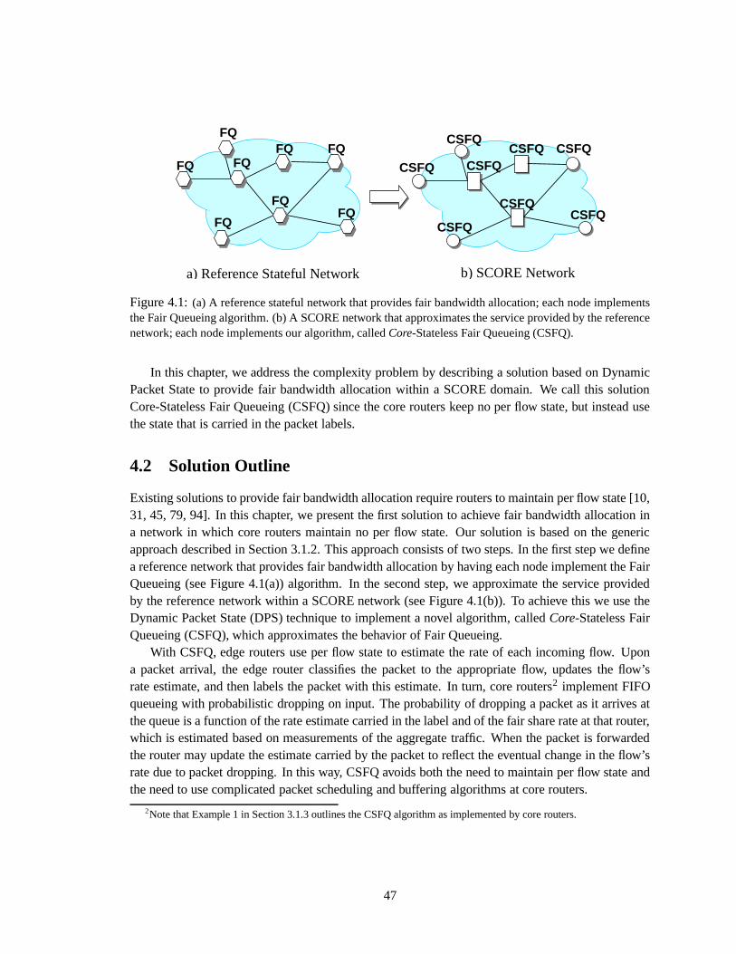
a) Reference Stateful Network b) SCORE Network

FQ

FQ FQ

FQFQ

FQFQ

FQ

CSFQ

CSFQ

CSFQ

CSFQ

CSFQ CSFQ

CSFQCSFQ

Figure 4.1: (a) A reference stateful network that provides fair bandwidth allocation; each node implementsthe Fair Queueing algorithm. (b) A SCORE network that approximates the service provided by the referencenetwork; each node implements our algorithm, called Core-Stateless Fair Queueing (CSFQ).

In this chapter, we address the complexity problem by describing a solution based on DynamicPacket State to provide fair bandwidth allocation within a SCORE domain. We call this solutionCore-Stateless Fair Queueing (CSFQ) since the core routers keep no per flow state, but instead usethe state that is carried in the packet labels.

4.2 Solution Outline

Existing solutions to provide fair bandwidth allocation require routers to maintain per flow state [10,31, 45, 79, 94]. In this chapter, we present the first solution to achieve fair bandwidth allocation ina network in which core routers maintain no per flow state. Our solution is based on the genericapproach described in Section 3.1.2. This approach consists of two steps. In the first step we definea reference network that provides fair bandwidth allocation by having each node implement the FairQueueing (see Figure 4.1(a)) algorithm. In the second step, we approximate the service providedby the reference network within a SCORE network (see Figure 4.1(b)). To achieve this we use theDynamic Packet State (DPS) technique to implement a novel algorithm, called Core-Stateless FairQueueing (CSFQ), which approximates the behavior of Fair Queueing.

With CSFQ, edge routers use per flow state to estimate the rate of each incoming flow. Upona packet arrival, the edge router classifies the packet to the appropriate flow, updates the flow’srate estimate, and then labels the packet with this estimate. In turn, core routers2 implement FIFOqueueing with probabilistic dropping on input. The probability of dropping a packet as it arrives atthe queue is a function of the rate estimate carried in the label and of the fair share rate at that router,which is estimated based on measurements of the aggregate traffic. When the packet is forwardedthe router may update the estimate carried by the packet to reflect the eventual change in the flow’srate due to packet dropping. In this way, CSFQ avoids both the need to maintain per flow state andthe need to use complicated packet scheduling and buffering algorithms at core routers.

2Note that Example 1 in Section 3.1.3 outlines the CSFQ algorithm as implemented by core routers.

47

4.3 Core-Stateless Fair Queueing (CSFQ)

In this section we present our algorithm, called Core-Stateless Fair Queueing (CSFQ), which ap-proximates the behavior of Fair Queueing in a SCORE network. To offer intuition about how CSFQworks, we first present the idealized bit-by-bit or fluid version of the probabilistic dropping scheme,and then extend the algorithm to a practical packet-by-packet version.

4.3.1 Fluid Model Algorithm

We first consider a bufferless fluid model of a router with output link speed � , where the flows aremodelled as a continuous stream of bits. We assume each flow’s arrival rate �

� � � is known precisely.

Max-min fair bandwidth allocations are characterized by the fact that all flows that are bottlenecked(i.e., have bits dropped) by this router have the same output rate. We call this rate the fair share rateof the server; let � � � � be the fair share rate at time � . In general, if max-min bandwidth allocationsare achieved, each flow � receives service at a rate given by �� �� � �

� � � � � � � � � . Let

� � � � denote thetotal arrival rate:

� � � � � ��� = �

� � � . If

� � � ����� then the fair share � � � � is the unique solution to

� �

� � =�� �� � �

� � � � � � � � � � (4.1)

If� � � � � � then no bits are dropped and we will, by convention, set � � � � � �����

�

� � � .

If �

� � � � � � � � , i.e., flow � sends no more than the server’s fair share rate, all of its traffic will

be forwarded. If �

� � ��� � � � � , then a fraction �

� ���;�� �����

�� ��� of its bits will be dropped, so it will have

an output rate of exactly � � � � . This suggests a very simple probabilistic forwarding algorithm thatachieves fair allocation of bandwidth: each incoming bit of flow � is dropped with the probability

����� � ��� �� � � � ��

� � �

�(4.2)

When these dropping probabilities are used, the arrival rate of flow � at the next hop is given by�� ���� �� � � � � � � ��� .

4.3.2 Packet Algorithm

The above algorithm is defined for a bufferless fluid system in which the arrival rates are knownexactly. Our task now is to extend this approach to the situation in real routers where transmissionis packetized, there is substantial buffering, and the arrival rates are not known.

We still employ a drop-on-input scheme, except that now we drop packets rather than bits.Because the rate estimation (described below) incorporates the packet size, the dropping probabilityis independent of the packet size and depends only, as above, on the rate �

� � � and fair share rate� � � � .

We are left with two remaining challenges: estimating the rates �

� � � and the fair share � � � � . We

address these two issues in turn in the next two subsections, and then discuss the rewriting of thelabels. Pseudocode reflecting this algorithm is described in Figures 4.3 and 4.4.

48

rate estimator +packet labeling

rate estimator +packet labeling

...packet dropping

estimator

buffer occupancy

arrival &departurerates

D

Flow 1

Flow n

ingress router

core/egress router

...

Figure 4.2: The architecture of the output port of an edge router, and a core router, respectively.

4.3.2.1 Computation of Flow Arrival Rate

Recall that in our architecture, the rates �

� � � are estimated at the edge routers and then these rates

are inserted into the packet labels. At each edge router, we use exponential averaging to estimate therate of a flow. Let ���

and ���

be the arrival time and length of the

� ���packet of flow � . The estimated

rate of flow � , �, is updated every time a new packet is received:

�

����

� ��� ' ; � �� � ��� � � ' ; � �� �������

�

(4.3)

where ��� ���

�)� ��;>=and � is a constant. We discuss the rationale for using the form ' ;

���

forthe exponential weight in Section 4.3.7.

4.3.2.2 Link Fair Rate Estimation

In this section, we present an estimation algorithm for � � � � . To give intuition, consider again thefluid model in Section 4.3.1 where the arrival rates are known exactly, and assume the system per-forms the probabilistic dropping algorithm according to Eq. (4.2). Then, the rate with which thealgorithm accepts packets is a function of the current estimate of the fair share rate, which we de-note by �� � � � . Letting 8 � �� � � � � denote this acceptance rate, we have

8 � �� � � � � �� � =�� �� � �

� � � � �� � � � �(� (4.4)

Note that 8 ��� � is a continuous, nondecreasing, concave, and piecewise-linear function of �� . If thelink is congested (

� � � � � � ) we choose �� � � � to be the unique solution to 8 ��� � � � . If the linkis not congested (

� � � ��� ) we take �� � � � to be the largest rate among the flows that traverse the

link, i.e., �� � � �!� �����=��

��� �� � � � . From Eq. (4.4) note that if we knew the arrival rates �

� � � we

could then compute � � � � directly. To avoid having to keep such per flow state, we seek instead toimplicitly compute �� � � � by using only aggregate measurements of 8 and

�.

We use the following heuristic algorithm with three aggregate state variables: �� , the estimatefor the fair share rate; �� , the estimated aggregate arrival rate; �8 , the estimated rate of the accepted

49

on packet � arrivalif (edge router)� � classify(� );� � ��� ����� � estimate rate( � � � � ); ��� use Eq. (4.3) � �

� �� � � max( � � � � � � �������� );if (� �� � � unif rand(0, 1))� � estimate � (� � );drop(p);

else� � estimate � (� � � );enqueue(p);

if (� �� � � � )� � ��� ����� � � ; ��� relabel p � �

Figure 4.3: The pseudocode of CSFQ.

traffic. The last two variables are updated upon the arrival of each packet. For �� we use exponentialaveraging with a parameter '#;

�� ��where is the inter-arrival time between the current and the

previous packet:

�� � ��� � ��� ' ; �� � � � � ' ; �� � �� ����� (4.5)

where ����� � is the value of �� before the updating. We use an analogous formula to update �8 .

The updating rule for �� depends on whether the link is congested or not. To filter out the esti-mation inaccuracies due to exponential smoothing we use a window of size ��� . A link is assumedto be congested, if ���� � at all times during an interval of length ��� . Conversely, a link is assumedto be uncongested, if �� � � at all times during an interval of length ��� . The value �� is updatedonly at the end of an interval in which the link is either congested or uncongested according tothese definitions. If the link is congested then �� is updated based on the equation 8 � �� �/� � . Weapproximate 8 ��� � by a linear function that intersects the origin and has slope �8 � �� ����� . This yields

�� � ��� � �� ����� � �8 (4.6)

If the link is not congested, �� � ��� is set to the largest rate of any active flow (i.e., the largest labelseen) during the last ��� time units. The value of �� � ��� is then used to compute dropping probabil-ities, according to Eq. (4.2). For completeness, we give the pseudocode of the CSFQ algorithm inFigure 4.4.

We now describe two minor amendments to this algorithm related to how the buffers are man-aged. The goal of estimating the fair share �� is to match the accepted rate to the link bandwidth. Dueto estimation inaccuracies, load fluctuations between �� ’s updates, and the probabilistic nature of ouralgorithm, the accepted rate may occasionally exceed the link capacity. While ideally the router’sbuffers can accommodate the extra packets, occasionally the router may be forced to drop the in-coming packet due to lack of buffer space. Since drop-tail behavior will defeat the purpose of ouralgorithm, and may exhibit undesirable properties in the case of adaptive flows such as TCP [37], it

50

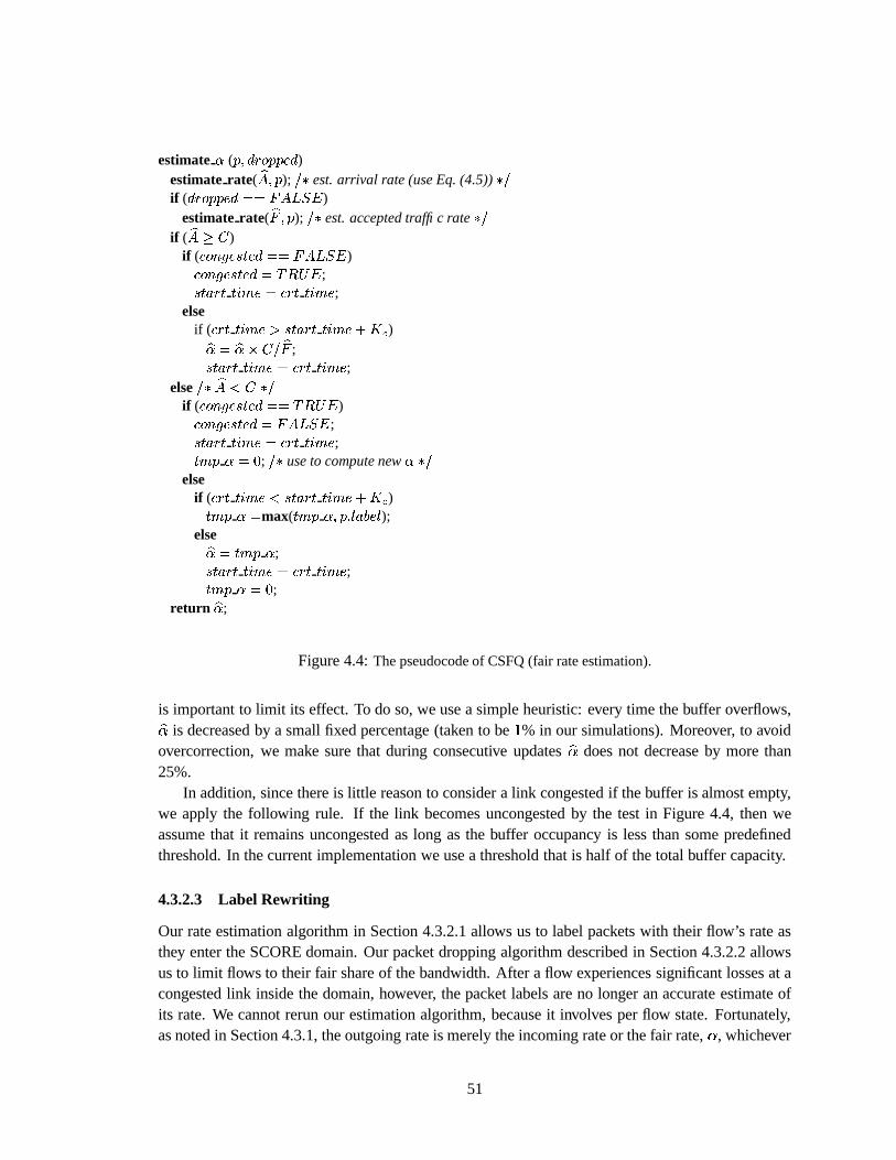
estimate � (� ���)�� � � ��� )estimate rate( �� � � ); ��� est. arrival rate (use Eq. (4.5)) � �if ( ���� � � ��� � ��� ��� 1 )

estimate rate( �� � � ); ��� est. accepted traffic rate � �if ( �� ��� )

if ( � ��� � �-+ ��� � ��� ��� 1� ) �� ��� � �-+ ��� � � ���� ;��+ � � + + �%� � �� � + + �%� � ;

elseif ( � + + �%� � � �-+ � � + + �%� ����� � )�� � �������� �� ;�-+ � � + + � � � �� � + + �%� � ;

else � � �� ��� � �if ( � ��� � �-+ ��� � � � ���� ) �� ��� � �-+ ��� ��� ��� 1� ;��+ � � + + �%� � �� � + + �%� � ;+�� � � ��� ; � � use to compute new � ��

elseif ( � + + �%� � � �-+ � � + + �%� ����� � )+�� � � � max( +�� � � � � � � ������ );

else�� � +�� � � ;�-+ � � + + � � � �� � + + �%� � ;+�� � � � � ;

return �� ;

Figure 4.4: The pseudocode of CSFQ (fair rate estimation).

is important to limit its effect. To do so, we use a simple heuristic: every time the buffer overflows,�� is decreased by a small fixed percentage (taken to be % in our simulations). Moreover, to avoidovercorrection, we make sure that during consecutive updates �� does not decrease by more than25%.

In addition, since there is little reason to consider a link congested if the buffer is almost empty,we apply the following rule. If the link becomes uncongested by the test in Figure 4.4, then weassume that it remains uncongested as long as the buffer occupancy is less than some predefinedthreshold. In the current implementation we use a threshold that is half of the total buffer capacity.

4.3.2.3 Label Rewriting

Our rate estimation algorithm in Section 4.3.2.1 allows us to label packets with their flow’s rate asthey enter the SCORE domain. Our packet dropping algorithm described in Section 4.3.2.2 allowsus to limit flows to their fair share of the bandwidth. After a flow experiences significant losses at acongested link inside the domain, however, the packet labels are no longer an accurate estimate ofits rate. We cannot rerun our estimation algorithm, because it involves per flow state. Fortunately,as noted in Section 4.3.1, the outgoing rate is merely the incoming rate or the fair rate, � , whichever

51

is smaller. Therefore, we rewrite the the packet label � as

� � � � � �� �� ��� ��� �� � � � (4.7)

By doing so, the outgoing flow rates will be properly represented by the packet labels.

4.3.3 Weighted CSFQ

The CSFQ algorithm can be extended to support flows with different weights. Let �

denote theweight of flow � . Returning to our fluid model, the meaning of these weights is that we say a fairallocation is one in which all bottlenecked flows have the same value for �� . Then, if

� � � � ��� , the

normalized fair rate � � � � is the unique value such that ��� = �

�� ���� � � �� �� � � . The expression

for the dropping probabilities in the weighted case is ����� � ��� �� � � � � . The only other major

change is that the label is now �

���, instead simply �

. Finally, without going into detail we note

that the weighted packet-by-packet version is virtually identical to the corresponding version of theplain CSFQ algorithm.

It is also important to note that with weighted CSFQ we can only approximate a reference net-work in which each flow has the same weight at all routers along its path. That is, our algorithm can-not accommodate situations where the relative weights of flows differ from router to router withina domain. However, even with this limitation, weighted CSFQ may prove a valuable mechanism inimplementing differential services, such as the one proposed in [116].

4.3.4 Performance Bounds

We now present the main theoretical result for CSFQ. For generality, this result is given for weightedCSFQ. The proof is given in Appendix A.

Our algorithm is built around several estimation procedures, and thus is inherently inexact. Onenatural concern is whether a flow can purposely “exploit” these inaccuracies to get more than itsfair share of bandwidth. We cannot answer this question with full generality, but we can analyze asimplified situation where the normalized fair share rate, � , is held fixed and there is no buffering,so the drop probabilities are precisely given by Eq. (4.2). In addition, we assume that when a packetarrives, a fraction of that packet equal to the flow’s forwarding probability is transmitted. Note thatduring any time interval � � =

� � � � a flow with weight � is entitled to receive at most � � � � � � � = �service time; we call any amount above this the excess service. This excess service can be bound,independent of both the arrival process and the length of the time interval during which the flow isactive. The bound does depend crucially on the maximal rate,

�, at which a flow packets can arrive

at a router (limited, for example, by the speed of the flow’s access link); the smaller this rate�

, thetighter the bound.

Theorem 1 Consider a link with a constant normalized fair rate � , and a flow with weight � . Then,the excess service received by a flow with weight � that sends at a rate no larger than

�is bounded

above by

� � �� � ln

�

� �

� � ��� � � (4.8)

52

where � � � � � , and � ����� represents the maximum length of a packet.

By bounding the excess service, we have shown that in this idealized setting, the asymptoticthroughput cannot exceed the fair share rate. Thus, flows can only exploit the system over shorttime scales; they are limited to their fair share over long time scales.

4.3.5 Implementation Complexity

At core routers, both the time and space complexity of our algorithm are constant with respect to thenumber of competing flows, and thus we think CSFQ could be implemented in very high speed corerouters. At each edge router CSFQ needs to maintain per flow state. Upon the arrival of each packet,the edge router needs to (1) classify the packet to a flow, (2) update the fair share rate estimation forthe corresponding outgoing link, (3) update the flow rate estimation, and (4) label the packet. Allthese operations with the exception of packet classification can be efficiently implemented today.

Efficient and general-purpose packet classification algorithms are still under active research. Weexpect to leverage these results. We also note that packet classification at ingress nodes is needed fora number of other purposes, such as in the context of Multiprotocol Label Switching (MPLS) [17]or for accounting purposes. Therefore, the classification required for CSFQ may not be an extracost. In addition, edge routers typically not on the high-speed backbone links pose no problem asclassification at moderate speeds is quite practical.

4.3.6 Architectural Considerations

We have used the term flow without defining what we mean. This was intentional, as the CSFQapproach can be applied to varying degrees of flow granularity; that is, what constitutes a flow isarbitrary as long as all packets in the flow follow the same path within the core. For convenience,flow as used here is implicitly defined as a source-destination pair, but one could easily assign fairrates to many other granularities such as source-destination-ports. Moreover, the unit of “flow” canvary from domain to domain as long as the rates are re-estimated when entering a new domain.

Similarly, we have not been precise about the size of the SCORE domains. In one extreme, wecould take each router as a domain and estimate rates at every router; this would allow us to avoidthe use of complicated per flow scheduling and dropping algorithms, but would require per flowclassification. Another possibility is that ISPs could extend their SCORE domain to the very edgeof their network, having their edge routers at the points where customer’s packets enter the ISP’snetwork. Building on the previous scenario, multiple ISPs could combine their domains so thatclassification and estimation did not have to be performed at ISP-ISP boundaries. The key obstaclehere is one of trust between ISPs.

4.3.7 Miscellaneous Details

Having presented the basic CSFQ algorithm, we now return to discuss a few aspects in more detail.We have used exponential averaging to estimate the arrival rate in Eq. (4.3). However, instead of

using a constant exponential weight we used ' ;��

, where is the inter-packet arrival time and �is a constant. Our motivation was that '7;

�� more closely reflects a fluid averaging process which

53

is independent of the packetizing structure. More specifically, it can be shown that if a constantweight is used, the estimated rate will be sensitive to the packet length distribution and there arepathological cases where the estimated rate differs from the real arrival rate by a factor; this wouldallow flows to exploit the estimation process and obtain more than their fair share. In contrast, byusing a parameter of ' ;

�� , the estimated rate will asymptotically converge to the real rate, and

this allows us to bound the excess service that can be achieved (as in Theorem 1). We used a similaraveraging process in Eq. (4.5) to estimate the total arrival rate

�.

The choice of � in the above expression '7;��

presents us with several tradeoffs. First, whilea smaller � increases system responsiveness to rapid rate fluctuations, a larger � better filters noiseand avoids potential system instability. Second, � should be large enough such that the estimatedrate, calculated at the edge of the network, remains reasonably accurate after a packet traversesmultiple links. This is because the delay-jitter changes the packets’ inter-arrival pattern, which mayresult in an increased discrepancy between the estimated rate (received in the packets’ labels) andthe real rate. To counteract this effect, as a rule of thumb, � should be one order of magnitudelarger that the delay-jitter experienced by a flow over a time interval of the same size, � . Third, �should be no larger than the average duration of a flow. Based on this constraints, an appropriatevalue for � would be between 100 and 500 ms.

4.4 Simulation Results

In this section we evaluate our algorithm by simulation. To provide some context, we compareCSFQ’s performance to three additional algorithms. Two of these, FIFO and RED, represent base-line cases where routers do not attempt to achieve fair bandwidth allocations. The other two algo-rithms, FRED and DRR, represent different approaches to achieving fairness.

� FIFO (First In First Out) - Packets are served in a first-in first-out order, and the buffers aremanaged using a simple drop-tail strategy; i.e., incoming packets are dropped when the bufferis full.

� RED (Random Early Detection) - Packets are served in a first-in first-out order, but the buffermanagement is significantly more sophisticated than drop-tail. RED [37] starts to probabilis-tically drop packets long before the buffer is full, providing early congestion indication toflows which can then gracefully back-off before the buffer overflows. RED maintains twobuffer thresholds. When the exponentially averaged buffer occupancy is smaller than the firstthreshold, no packet is dropped, and when the exponentially averaged buffer occupancy islarger than the second threshold all packets are dropped. When the exponentially averagedbuffer occupancy is between the two thresholds, the packet dropping probability increaseslinearly with buffer occupancy.

� FRED (Fair Random Early Drop) - This algorithm extends RED to provide some degree offair bandwidth allocation [67]. To achieve fairness, FRED maintains state for all flows thathave at least one packet in the buffer. Unlike RED where the dropping decision is based onlyon the buffer state, in FRED dropping decisions are based on this flow state. Specifically,FRED preferentially drops a packet of a flow that has either (1) had many packets dropped

54

in the past, or (2) a queue larger than the average queue size. FRED has two variants (whichwe will call FRED-1 and FRED-2). The main difference between the two is that FRED-2guarantees to each flow a minimum number of buffers. As a general rule, FRED-2 performsbetter than FRED-1 only when the number of flows is large. In the following data, when wedon’t distinguish between the two, we are quoting the results from the version of FRED whichperformed the best.

� DRR (Deficit Round Robin) - This algorithm represents an efficient implementation of thewell-known weighted fair queueing (WFQ) discipline. The buffer management scheme as-sumes that when the buffer is full the packet from the longest queue is dropped. DRR is theonly one of the four to use a sophisticated per-flow queueing algorithm, and thus achieves thehighest degree of fairness.

These four algorithms represent four different levels of complexity. DRR and FRED have toclassify incoming flows, whereas FIFO and RED do not. In addition, DRR has to implement itspacket scheduling algorithm (whereas the rest all use first-in-first-out scheduling). CSFQ edgerouters have complexity comparable to FRED, and CSFQ core routers have complexity comparableto RED.

We have examined the behavior of CSFQ under a variety of conditions. We use an assortmentof traffic sources (mainly CBR and TCP, but also some on-off sources) and topologies. For spacereasons, we only report on a small sampling of the simulations we have run; a fuller set of tests, andthe scripts used to run them, is available at http://www.cs.cmu.edu/˜istoica/csfq. Allsimulations were performed in ns-2 [78], which provides accurate packet-level implementation forvarious network protocols, such as TCP and RLM (Receiver-driven Layered Multicast) [69], andvarious buffer management and scheduling algorithms, such as RED and DRR.

Unless otherwise specified, we use the following parameters for the simulations in this section.Each output link has a latency of 1 ms, a buffer of 64 KB, and a buffer threshold for CSFQ of 16KB. In the RED and FRED cases, the first threshold is set to 16 KB, while the second one is set to32 KB. The averaging constant used in estimating the flow rate is �*� � � ms, while the averagingconstant used in estimation the fair rate � is � � � � � � ms. Finally, in all topologies we use the firstrouter (gateway) on the path of a flow is always assumed to be the edge router; all other routers areassumed without exception to be core routers.

We simulated the other four algorithms to give us benchmarks against which to assess theseresults. We use DRR as our model of fairness and use the baseline cases, FIFO and RED, as repre-senting the (unfair) status quo. The goal of these experiments is determine where CSFQ sits betweenthese two extremes. FRED is a more ambiguous benchmark, being somewhat more complex thanCSFQ, but not as complex as DRR.

In general, we find that CSFQ achieves a reasonable degree of fairness, significantly closerto DRR than to FIFO or RED. CSFQ’s performance is typically comparable to FRED’s, althoughthere are a few situations where CSFQ significantly outperforms FRED. There are a large number ofexperiments and each experiment involves rather complex dynamics. Due to space limitations, in thesections that follow we will merely highlight a few important points and omit detailed explanationsof the dynamics.

55

Flow 0

Flow 1

Flow N-1

.

.

.

Sink

Router

Sources

(a)

0

0.2

0.4

0.6

0.8

1

5 10 15 20 25 30

Ban

dwid

th (

Mbp

s)

Flow Number

DRRCSFQ

FRED-1FRED-2

REDFIFO

(b)

Figure 4.5: (a) A 10 Mbps link shared by N flows. (b) The average throughput over 10 sec when N = 32, andall flows are CBRs. The arrival rate for flow i is (i + 1) times larger than its fair share. The flows are indexedfrom 0.

4.4.1 A Single Congested Link

We first consider a single congested link shared by�

flows (see Figure 4.5(a)). We performed threerelated experiments.

In the first experiment, we have 32 CBR flows, indexed from 0, where flow � sends � � timesmore than its fair share of 0.3125 Mbps. Thus flow 0 sends 0.3125 Mbps, flow 1 sends 0.625 Mbps,and so on. Figure 4.5(b) shows the average throughput of each flow over a 10 sec interval; FIFO,RED, and FRED-1 fail to ensure fairness, with each flow getting a share proportional to its incomingrate, while DRR is extremely effective in achieving a fair bandwidth distribution. CSFQ and FRED-2 achieve a less precise degree of fairness; for CSFQ the throughputs of all flows are between � � %and � � % of the ideal value.

In the second experiment we consider the impact of an ill-behaved CBR flow on a set of TCPflows. More precisely, the traffic of flow 0 comes from a CBR source that sends at 10 Mbps, while allthe other flows (from 1 to 31) are TCPs. Figure 4.6(a) shows the throughput of each flow averagedover a 10 sec interval. The only two algorithms that can most effectively contain the CBR floware DRR and CSFQ. Under FRED the CBR flow gets almost 1.8 Mbps – close to six times morethan its fair share – while the CBR only gets 0.396 Mbps and 0.355 Mbps under DRR and CSFQ,respectively. As expected, FIFO and RED perform poorly, with the CBR flow getting over 8 Mbpsin both cases.

In the final experiment, we measure how well the algorithms can protect a single TCP flowagainst multiple ill-behaved flows. We perform � simulations, each for a different value of

�,

� � � � � � . In each simulation we take one TCP flow and�

CBR flows; each CBR sends attwice its fair share rate of =

�� �=Mbps. Figure 4.6(b) plots the ratio between the average throughput

of the TCP flow over 10 sec and the total bandwidth it should receive as a function of the totalnumber of flows in the system

� � . There are three points of interest. First, DRR performsvery well when there are less than 22 flows, but its performances decreases afterwards becausethen the TCP flow’s buffer share is less than three buffers which is known to significantly affect its

56

0

0.2

0.4

0.6

0.8

1

1.2

1.4

1.6

1.8

5 10 15 20 25 30

Ban

dwid

th (

Mbp

s)

Flow Number

DRRCSFQFRED

REDFIFO

(a)

0

0.2

0.4

0.6

0.8

1

1.2

1.4

5 10 15 20 25 30

Allo

cate

d B

wdt

h. /

Idea

l Bw

dth.

Total Number of Flows

DRRCSFQFRED

REDFIFO

(b)

Figure 4.6: (a) The throughputs of one CBR flow (0 indexed) sending at 10 Mbps, and of 31 TCP flowssharing a 10 Mbps link. (b) The normalized bandwidth of a TCP flow that competes with

�CBR flows

sending at twice their allocated rates, as a function of�

.

throughput. Second, CSFQ performs better than DRR when the number of flows is large. This isbecause CSFQ is able to cope better with the TCP burstiness by allowing the TCP flow to have morethan two packets buffered for short time intervals. Finally, across the entire range, CSFQ providessimilar or better performance as compared to FRED.

4.4.2 Multiple Congested Links

We now analyze how the throughput of a well-behaved flow is affected when the flow traverses morethan one congested link. We performed two experiments based on the topology shown in Figure 4.7.All CBRs, except CBR-0, send at 2 Mbps. Since each link in the system has 10 Mbps capacity, thiswill result in all links between routers being congested.

In the first experiment, we have a CBR flow (denoted CBR-0) sending at its fair share rateof 0.909 Mbps. Figure 4.8(a) shows the fraction of CBR-0’s traffic that is forwarded, versus thenumber of congested links. CSFQ and FRED perform reasonably well, although not quite as wellas DRR.

In the second experiment we replace CBR-0 with a TCP flow. Similarly, Figure 4.8(b) plots thenormalized TCP throughput against the number of congested links. Again, DRR and CSFQ proveto be effective. In comparison, FRED performs significantly worse though still much better thanRED and FIFO. The reason is that while DRR and CSFQ tries to allocate bandwidth fairly amongcompeting flows during congestion, FRED tries to allocate the buffer fairly. Flows with differentend-to-end congestion control algorithms will achieve different throughputs even if routers try tofairly allocate the buffer. In the case of Figure 4.8(a), all sources are CBR, i.e., none are adoptingany end-to-end congestion control algorithms, FRED provides performance similar to CSFQ andDRR. In the case of Figure 4.8(b), a TCP flow is competing with multiple CBR flows. Since the TCPflow slows down during congestion while CBQ does not, it achieves significantly less throughputthan a competing CBR flow.

57

CBR-1

Router2Router1 Router K Router K+1

... ... ...

CBR-10 CBR-11 CBR-20 CBR-K1 CBR-K10

CBR-1 – CBR-10 CBR-K1 – CBR-K10

CBR/TCP-0 CBR/TCP-0

Source Sink

Sinks

Sources

...

Figure 4.7: Topology for analyzing the effects of multiple congested links on the throughput of a flow. Eachlink has ten cross flows (all CBRs). All links have 10 Mbps capacities. The sending rates of all CBRs,excepting CBR-0, are 2 Mbps, which leads to all links between routers being congested.

0

0.2

0.4

0.6

0.8

1

1.2

1.4

1 2 3 4 5

Allo

cate

d B

wdt

h. /

Idea

l Bw

dth.

Number of Congested Links

DRRCSFQFRED

REDFIFO

(a)

0

0.2

0.4

0.6

0.8

1

1.2

1.4

1 2 3 4 5

Allo

cate

d B

wdt

h. /

Idea

l Bw

dth.

Number of Congested Links

DRRCSFQFRED

REDFIFO

(b)

Figure 4.8: (a) The normalized throughput of CBR-0 as a function of the number of congested links. (b)The same plot when CBR-0 is replaced by a TCP flow.

4.4.3 Coexistence of Different Adaptation Schemes

In this experiment we investigate the extent to which CSFQ can deal with flows that employ differentadaptation schemes. Receiver-driven Layered Multicast (RLM) [69] is an adaptive scheme in whichthe source sends the information encoded into a number of layers (each to its own multicast group)and the receiver joins or leaves the groups associated with the layers based on how many packetdrops it is experiencing. We consider a 4 Mbps link traversed by one TCP and three RLM flows.Each source uses a seven layer encoding, where layer � sends �

� Kbps; each layer is modeled by

a CBR traffic source. The fair share of each flow is 1Mbps. In the RLM case this will correspond toeach receiver subscribing to the first five layers. 3

The average receiving rates averaged over 1 sec intervals for each algorithm are plotted in Fig-ure 4.9. We have conducted two separate simulations of CSFQ.4 In the first one, we have used thesame averaging constant as in the rest of this chapter: � � � � ms, and � � � � � � ms. Here, one

3More precisely, we have ��� ���� ��� Kbps � � ��� � Mbps.

4See also [69] for additional simulations of RLM and TCP.

58

0

0.5

1

1.5

2

2.5

3

3.5

4

0 50 100 150 200 250 300 350 400 450

Thr

ough

put (

Mbp

s)

Time (sec)

TCPRLM1RLM2RLM3

(a) DRR

0

0.5

1

1.5

2

2.5

3

3.5

4

0 50 100 150 200 250 300 350 400 450

Thr

ough

put (

Mbp

s)

Time (sec)

TCPRLM1RLM2RLM3

(c) CSFQ ( � � � � ms, � � � � � � ms.)

0

0.5

1

1.5

2

2.5

3

3.5

4

0 50 100 150 200 250 300 350 400 450

Thr

ough

put (

Mbp

s)

Time (sec)

TCPRLM1RLM2RLM3

(e) RED

0

0.5

1

1.5

2

2.5

3

3.5

4

0 50 100 150 200 250 300 350 400 450

Thr

ough

put (

Mbp

s)

Time (sec)

TCPRLM1RLM2RLM3

(b) FRED

0

0.5

1

1.5

2

2.5

3

3.5

0 50 100 150 200 250 300 350 400 450

Thr

ough

put (

Mbp

s)

Time (sec)

TCPRLM1RLM2RLM3

(d) CSFQ ( � � � � ms, ��� � � � ms.)

0

0.5

1

1.5

2

2.5

3

3.5

4

0 50 100 150 200 250 300 350 400 450

Thr

ough

put (

Mbp

s)

Time (sec)

TCPRLM1RLM2RLM3

(f) FIFO

Figure 4.9: The throughputs of three RLM flows and one TCP flow along a 4 Mbps link.

59

RLM flow does not get its fair share (it is one layer below where it should be). We think this is dueto the bursty behavior of the TCP that is not detected by CSFQ soon enough, allowing the TCP toopportunistically grab more bandwidth than its share at the expense of less aggressive RLM flows.To test this hypothesis, we have changed the averaging time intervals to � � � � ms, and � � � � �ms, respectively, which result in TCP flow bandwidth being restricted much earlier. As shown inFigure 4.9(d), with these parameters all flows receive roughly 1 Mbps.

An interesting point to notice is that FRED does not provide fair bandwidth allocation in thisscenario. Again, as discussed in Section 4.4.2, this is due to the fact that RLM and TCP use differentend-to-end congestion control algorithms.

Finally, we note that we have performed two other similar experiments (not included here dueto space limitations): one in which the TCP flow is replaced by a CBR that sends at 4 Mbps, andanother in which we have both the TCP and the CBR flows together along with the three RLM flows.The overall results were similar, except that in both experiments all flows received their shares underCSFQ when using the original settings for the averaging intervals, i.e., � � � � ms and � � � � � �ms. In addition, in some of these other experiments where the RLM flows are started before theTCP, the RLM flows get more than their share of bandwidth when RED and FIFO are used.

4.4.4 Different Traffic Models

So far we have only considered CBR and TCP traffic sources. We now look at two additionalsource models with greater degrees of burstiness. We again consider a single 10 Mbps congestedlink. In the first experiment, this link is shared by one ON-OFF source and 19 CBRs that send atexactly their share, 0.5 Mbps. The ON and OFF periods of the ON-OFF source are both drawn fromexponential distributions with means of 200 ms and 19*200 ms respectively. During the ON periodthe ON-OFF source sends at 10 Mbps. Note that the ON-time is on the same order as the averaginginterval �*� � � ��� � for CSFQ’s rate estimation algorithm, so this experiment is designed to test towhat extent CSFQ can react over short time scales.

Algorithm delivered droppedDRR 1080 3819CSFQ 1000 3889FRED 1064 3825RED 2819 2080FIFO 3771 1128

Table 4.1: Statistics for an ON-OFF flow with 19 Competing CBRs flows (all numbers are in packets)

The ON-OFF source sent 4899 packets over the course of the experiment. Table 4.1 shows thenumber of packets from the ON-OFF source dropped at the congested link. The DRR results showwhat happens when the ON-OFF source is restricted to its fair share at all times. FRED and CSFQalso are able to achieve a high degree of fairness.

Our next experiment simulates Web traffic. There are 60 TCP transfers whose inter-arrival timesare exponentially distributed with the mean of 0.1 ms, and the length of each transfer is drawn froma Pareto distribution with a mean of 40 packets (1 packet = 1 KB) and a shaping parameter of 1.06.

60

These values are consistent with those presented by Crovella and Bestavros [27]. In addition, thereis a single 10 Mbps CBR flow.

Algorithm mean time std. devDRR 46.38 197.35CSFQ 88.21 230.29FRED 73.48 272.25RED 790.28 1651.38FIFO 1736.93 1826.74

Table 4.2: The mean transfer times (in ms) and the corresponding standard deviations for 60 short TCPs inthe presence of a CBR flow that sends at the link capacity, i.e., 10 Mbps.

Table 4.2 presents the mean transfer time and the corresponding standard deviations. Here,CSFQ and FRED do less well than DRR, but one order of magnitude better than FIFO and RED.

4.4.5 Large Latency

All of our experiments so far have had minimal latencies. In this experiment we again consider asingle 10 Mbps congested link, but now the flows have propagation delays of 100 ms in getting tothe congested link. The load is comprised of one CBR that sends at the link capacity and 19 TCPflows. Table 4.3 shows the mean number of packets forwarded for each TCP flow during a 100 sectime interval. CSFQ and FRED both perform reasonably well.

4.4.6 Packet Relabeling

Recall that when the dropping probability�

of a packet is non-zero we relabel it with a new labelwhere � � ��� � � � � � � ����� so that the label of the packet will reflect the new rate of the flow. Totest how well this works in practice, we consider the topology in Figure 4.10, where each link is 10Mbps. Note that as long as all three flows attempt to use their full fair share, the fair shares of flows 1and 2 are less on link 2 (3.33 Mbps) than on link 1 (5 Mbps), so there will be dropping on both links.This will test the relabeling function to make sure that the incoming rates are accurately reflected onthe second link. We perform two experiments (only looking at CSFQ’s performance). In the first,there are three CBRs sending data at 10 Mbps each. Table 4.4 shows the average throughputs over

Algorithm mean std. devDRR 5857.89 192.86CSFQ 5135.05 175.76FRED 4967.05 261.23RED 628.10 80.46FIFO 379.42 68.72

Table 4.3: The mean throughput (in packets) and standard deviation for 19 TCPs in the presence of a CBRflow along a link with propagation delay of 100 ms. The CBR sends at the link capacity of 10 Mbps.

61

Flow 1(10 Mbps)

Flow 2(10 Mbps)

Flow 3(10 Mbps)

Sink

Router 2

Router 1

10 Mbps

10 Mbps

Link 1(10 Mbps)

Link 2(10 Mbps)

10 Mbps

Source

Figure 4.10: Simulation scenario for the packet relabeling experiment. Each link has 10 Mbps capacity, anda propagation delay of 1 ms.

Traffic Flow 1 Flow 2 Flow 3CBR 3.267 3.262 3.458TCP 3.232 3.336 3.358

Table 4.4: The throughputs resulting from CSFQ averaged over 10 sec for the three flows in Figure 4.10along link 2.

10 sec of the three CBR flows. As expected, these rates are closed to 3.33 Mbps. In the secondexperiment, we replace the three CBRs by three TCPs. Again, despite the TCP burstiness whichmay negatively affect the rate estimation and relabeling accuracy, each TCP gets its fair share.

4.4.7 Discussion of Simulation Results

We have tested CSFQ under a wide range of conditions; conditions purposely designed to stressits ability to achieve fair allocations. These tests, and the others we have run but cannot showhere because of space limitations, suggest that CSFQ achieves a reasonable approximation of fairbandwidth allocations in most conditions. Certainly CSFQ is far superior in this regard to the statusquo (FIFO or RED). Moreover, in all situations CSFQ is roughly comparable with FRED, and insome cases it achieves significantly fairer allocations. Recall that FRED requires per-packet flowclassification while CSFQ does not, so we are achieving these levels of fairness in a more scalablemanner. However, there is clearly room for improvement in CSFQ. We think our buffer managementalgorithm may not be well-tuned to the vagaries of TCP buffer usage, and so are currently lookingat adopting an approach closer in spirit to RED for buffer management, while retaining the use ofthe labels to achieve fairness.

4.5 Related Work

An alternative to the allocation approach was recently proposed to address the problem of the ill-behaved (unfriendly) flows. This approach is called the identification approach and it is best ex-emplified by Floyd and Fall [36]. In this approach, routers use a lightweight detection algorithmto identify unfriendly flows, and then explicitly manage the bandwidth of these unfriendly flows.This bandwidth management can range from merely restricting unfriendly flows to no more than

62

Simulation 1 Simulation 2Algorithm

UDP TCP-1 TCP-2 TCP-1 TCP-2REDI 0.906 0.280 0.278 0.565 0.891CSFQ 0.554 0.468 0.478 0.729 0.747

Table 4.5: Simulation 1 – The throughputs in Mbps of one UDP and two TCP flows along a 1.5 Mbps linkunder REDI [36] and CSFQ, respectively. Simulation 2 – The throughputs of two TCPs (where TCP-2 opensits congestion window three times faster than TCP-1), under REDI and CSFQ, respectively.

the currently highest friendly flow’s share to the extreme of severely punishing unfriendly flows bydropping all of their packets.

Compared to CSFQ, the solution to implementing the identification approach described by Floydand Fall [36] has several drawbacks. First, this solution requires routers to maintain state for eachflow that has been classified as un-friendly. In contrast, CSFQ does not require core routers tomaintain any per flow state. Second, designing accurate identification tests for unfriendly flows isinherently difficult. Finally, the identification approach requires that all flows to implement a similarcongestion control mechanism, i.e., to be TCP friendly. We believe that this is overly restrictive as itseverely limits the freedom of designing new congestion protocols that best suit application needs.

Next, we discuss in more detail the difficulty of providing accurate identification tests for un-friendly flows. One can think of the process of identifying unfriendly flows as occurring in twologically distinct stages. The first and relatively easy step is to estimate the arrival rate of a flow.The second, and harder, step is to use this arrival rate information (along with the dropping rate andother aggregate measurements) to decide if the flow is unfriendly. Assuming that friendly flows usea TCP-like adjustment method of increase-by-one and decrease-by-half, one can derive an expres-sion (see [36] for details) for the bandwidth share � as a function of the dropping rate � , round-triptime

�, and packet size � : ��� �

���� � for some constant . Because routers do not know the roundtrip time

�of flows, they use the lower bound of double the propagation delay of the attached link.

Unfortunately, this allows flows further away from the link to behave more aggressively withoutbeing identified as being unfriendly.

To see how this occurs in practice, consider the following two experiments using the identifica-tion algorithm described by Floyd and Fall [36], which we call RED with Identification (REDI).5

In each case there are multiple flows traversing a 1.5 Mbps link with a latency of 3 ms; the outputbuffer size is 32 KB and all constants � , � � , and � � , respectively, are set to 400 ms. Table 4.5shows the bandwidth allocations under REDI and CSFQ averaged over 100 sec. In the first experi-ment (Simulation 1), we consider a 1 Mbps UDP flow and two TCP flows; in the second experiment(Simulation 2) we have a standard TCP (TCP-1) and a modified TCP (TCP-2) that opens the con-gestion window three times faster. In both cases REDI fails to identify the unfriendly flow, allowingit to obtain almost two-thirds of the bandwidth. As we increase the latency of the congested link,REDI starts to identify unfriendly flows. However, for some values as high as 18 ms, it still fails toidentify such flows. Thus, the identification approach still awaits a viable realization and, as of now,

5We are grateful to Sally Floyd who provided us her script implementing the REDI algorithm. We used a similar scriptin our simulation, with the understanding that this is a preliminary design of the identification algorithm. Our contentionis that the design of such an identification algorithm is fundamentally difficult due to the uncertainty of RTT.

63

the allocation approach is the only demonstrated method able to deal with the problem of unfriendlyflows.

The problem of estimating fair-share rate has also been studied in the context of designingAvailable Bit Rate (ABR) algorithms for ATM networks. While the problems are similar, there arealso several important differences. First, in ATM ABR, the goal is to provide explicit feedback toend systems for policing purposes so that cell loss inside the network can be prevented. In CSFQ,there is no explicit feedback and edge policing. Packets from a flow may arrive at a much higherrate than the flow’s fair share rate and the goal of CSFQ is to ensure, by probabilistic dropping, thatsuch flows do not get more service than their shares. Second, since ATM already keeps per virtualcircuit (VC) state, additional per VC state is usually added to improve the accuracy and reduce thetime complexity of estimating the fair share rate [20, 33, 61]. However, there are several algorithmsthat try to estimate the fair share without keeping per flow state [87, 95]. These algorithms rely onthe flow rates communicated by the end-system. These estimates are assumed to remain accurateover multiple hops, due to the accurate explicit congestion control provided by ABR. In contrast, inCSFQ, since the number of dropped packets cannot be neglected, the flow rates are re-computed ateach router, if needed (see Section 4.3.2.3). In addition, the estimation algorithms are themselvesquite different. While the algorithms in averaging over the flow rates communicated by the end-systems, CSFQ uses linear interpolation in conjunction with exponentially averaging the trafficaggregates at the router. Our preliminary analysis and evaluation show that our estimation algorithmis more suited for our context.

4.6 Summary

In this chapter we have presented a solution that achieves fair bandwidth allocation, without re-quiring core routers to maintain any per-flow state. The key idea is to use the DPS technique toapproximate the service provided by a reference network — in which every node implements FairQueueing – within a SCORE network. Each node in the SCORE network implements a novel al-gorithm, called Core-Stateless Fair Queueing (CSFQ). With CSFQ edge routers estimate flow ratesand insert them into the packet headers. Core routers simply perform probabilistic dropping on in-put based on these labels and an estimate of the fair share rate, the computation of which requiresonly aggregate measurements. Packet labels are rewritten by the core routers to reflect output rates,so this approach can handle multi-hop situations.

We have tested CSFQ and several other algorithms under a wide variety of conditions. Wehave found that CSFQ achieves a significant degree of fairness in all of these circumstances. Whilenot matching the fairness benchmark of DRR, it is comparable or superior to FRED, and vastlybetter than the baseline cases of RED and FIFO. We know of no other approach that can achievecomparable levels of fairness without any per-flow operations in the core routers.

64

Chapter 5

Providing Guaranteed Services in SCORE

In the previous chapter we demonstrated that using the SCORE/DPS framework makes it possible toimplement a service with a per flow semantic (i.e., per flow isolation) in a stateless core architecture.In this chapter, we present a second example which shows that it is possible to provide per flowbandwidth and delay guarantees in a core stateless network. We achieve this goal by using the DPStechnique to implement the functionalities required by the Guaranteed service [93] on both the dataand control paths in a SCORE network.

The rest of this chapter is organized as follows. The next section presents the motivation behindthe Guaranteed service and describes the problems with the existing solutions. Section 5.2 outlinesour solution to implement the Guaranteed service in a SCORE network. Sections 5.3 and 5.4 presentdetails of both our data and control path algorithms. Section 5.5 describes a design and a prototypeimplementation of the proposed algorithms in IPv4 networks. Finally, Section 5.6 describes relatedwork, and Section 5.7 summarizes our findings.

5.1 Background

As new applications such as IP telephony, video-conferencing, audio and video streaming, anddistributed games are deployed in the Internet, there is a growing need to support more sophisticatedservices than the best-effort service. Unlike traditional applications such as file transfer, these newapplications have much stricter timeliness and bandwidth requirements. For example, in order toprovide a quality comparable to today’s telephone service, the end-to-end delay should not exceed100 ms [64]. Since in a global network the propagation delay alone is about 100 ms, meeting suchtight delay requirements is a challenging task [7]. Similarly, to provide high quality video and audiobroadcasting, it is desirable to be able to ensure both bandwidth and delay guarantees.

To support these new applications, the IETF has proposed two service models: the Guaranteedservice [93] defined in the context of Intserv [82], and the Premium service [76] defined in thecontext of Diffserv [32]. These services have important differences in both their semantic and im-plementation complexity. At the service definition level, while the Guaranteed service can provideboth per flow delay and bandwidth guarantees [93], the Premium service can provide only per flowbandwidth and per aggregate delay guarantees [76]. Thus, with the Premium service, if two flowshave different delay requirements, say

�= and

� � , the only way to meet both these delay require-ments is to ensure a delay of

�� �� �� � � = � � � � to both flows. The main drawback of this approach is

65

that it can result in very low resource utilization for the premium traffic. In particular, as we show inAppendix B.1, even if the fraction that can be allocated to the premium traffic on every link in thenetwork is very low (e.g., 10%), the queueing delay across a large network (e.g., 15 routers) can berelative large (e.g., 240 ms). In contrast, the Guaranteed service can achieve both higher resourceutilization and tighter delay bounds, by better matching flow requirements to resource usage.

At the implementation level, current solutions to provide guaranteed services require each routerto process per flow signaling messages and maintain per flow state on the control path, and toperform per flow classification, scheduling, and buffer management on the data path. Performingper flow management inside the network affects both the network scalability and robustness. Theformer is because the per flow operation complexity usually increases as a function of the numberof flows; the latter is because it is difficult to maintain the consistency of dynamic, and replicatedper flow state in a distributed network environment. While there are several proposals that aim toreduce the number of flows inside the network, by aggregating micro-flows that follow the samepath into one macro-flow [5, 49], they only alleviate this problem, but do not fundamentally solveit. This is because the number of macro flows can still be quite large in a network with many edgerouters, as the number of paths is a quadratic function of the number of edge nodes.

In contrast, the Premium service is implemented in the context of the Diffserv architecturewhich distinguishes between edge and core routers. While edge routers process packets on a perflow or per aggregate basis, core routers do not maintain any fine grained state about the traffic;they simply forward premium packets based on a high priority bit set in the packet headers byedge routers. Pushing the complexity to the edge and maintaining a simple core makes the dataplane highly scalable. However, the Premium service still requires admission control on the controlpath. One proposal is to use a centralized bandwidth broker that maintains the topology as wellas the state of all nodes in the network. In this case, the admission control can be implementedby the broker, eliminating the need for maintaining distributed reservation state. However, such acentralized approach is more appropriate for an environment where most flows are long lived, andset-up and tear-down events are rare.

In summary, the Guaranteed service is more powerful but has serious limitations with respectto network scalability and robustness. On the other hand, the Premium service is more scalable,but cannot achieve the levels of flexibility and utilization of the Guaranteed service. In addition,scalable and robust admission control for the Premium service is still an open research problem.

In this chapter we show that by using the SCORE/DPS framework we can achieve the bestof the two worlds: provide Guaranteed service semantic while maintaining the scalability and therobustness of the Diffserv architecture.

5.2 Solution Outline

Current solutions to implement the Guaranteed service assume a stateful network in which eachrouter maintains per flow state. The state is used by both the admission control module in thecontrol plane and the classifier and scheduler in the data plane.

In this chapter, we propose scheduling and admission control algorithms that provide the Guar-anteed service but do not require core routers to maintain per flow state. The main idea behind oursolution is to approximate a reference stateful network that provides the Guaranteed service in a

66

a) Reference Stateful Network b) SCORE Network

Jitter-VC

CJVC

CJVC

CJVC

CJVC

CJVC CJVC

CJVCCJVC

Jitter-VC

Jitter-VC

Jitter-VCJitter-VC

Jitter-VCJitter-VCJitter-VC

Figure 5.1: (a) A reference stateful network that provides the Guaranteed service [93]. Each node imple-ments the Jitter-Virtual Clock (Jitter-VC) algorithm on the data path, and per flow admission control on thecontrol path. (b) A SCORE network that emulates the service provided by the reference network. On the datapath, each node approximates Jitter-VC with a new algorithm, called Core-Jitter Virtual Clock (CJVC). Onthe control path each node approximates per flow admission control.

SCORE network (see Figure 5.1). The key technique used to implement these algorithms is Dy-namic Packet State (DPS). On the control path, our solution aims to emulate per flow admissioncontrol, while on the data path, our algorithm aims to emulate a reference network in which everynode implements the Delay-Jitter-Controlled Virtual Clock (Jitter-VC) algorithm.

Among many scheduling disciplines that can implement the Guaranteed service we chose Jitter-VC for several reasons. First, unlike various Fair Queueing algorithms [31, 79], in which a packet’sdeadline can depend on state variables of all active flows, in Jitter-VC a packet’s deadline dependsonly on the state variables of the flow it belongs to. This property of Jitter-VC makes the algorithmeasier to approximate in a SCORE network. In particular, the fact that packet’s deadline can becomputed exclusively based on the state variables of the flow it belongs to, makes it possible toeliminate the need to replicate and maintain per flow state at all nodes along the path. Instead, perflow state can be stored only at the ingress node, inserted into the packet header by the ingress node,and retrieved later by core nodes, which then use it to determine the packet’s deadline. Second, byregulating traffic inside the network using delay-jitter-controllers (discussed below), it can be shownthat with very high probability, the number of packets in the server at any given time is significantlysmaller than the number of flows (see Section 5.3.3). This helps to simplify the scheduler.

In the next section, we present techniques that eliminate the need for data plane algorithms touse per flow state at core nodes. In particular, at core nodes, packet classification is no longer neededand packet scheduling is based on the state carried in packet headers, rather than per flow state storedlocally at each node. In Section 5.4, we will show that fully distributed admission control can alsobe achieved without the need for maintaining per flow state at core nodes.

5.3 Data Plane: Scheduling Without Per Flow State

In this section, we first describe Jitter-VC, which is used to achieve guaranteed services in thereference network, and then present our algorithm, called Core-Jitter-VC (CJVC). CJVC uses theDynamic Packet State (DPS) technique to emulate Jitter-VC in a SCORE network. In Appendix B.3we present an analysis to show that a network of routers implementing CJVC provides the same

67

delay bound as a network of routers implementing the Jitter-VC algorithm.

5.3.1 Jitter Virtual Clock (Jitter-VC)

Jitter-VC is a non-work-conserving version of the Virtual Clock algorithm [127]. It uses a combina-tion of a delay-jitter rate-controller [112, 126] and a Virtual Clock scheduler. The algorithm worksas follows: each packet is assigned an eligible time and a deadline upon its arrival. The packet isheld in the rate-controller until it becomes eligible, i.e., the system time exceeds the packet’s eligibletime (see Figure 5.2(a)). The scheduler then orders the transmission of eligible packets accordingto their deadlines.

Notation Comments���� the � -th packet of flow ����� length of ���������� � arrival time of ���� at node

�

����� � time when ���� was sent by node�

� ���� � eligible time of � �� at node�

����� � deadline of ���� at node�

� ���� � time ahead of schedule: � ��� � ��� ���� � � � � � ���� ���� slack delay of ����

� � propagation delay between nodes�

and� �

� � transmission time of a maximum size packet at node�

Table 5.1: Notations used in Section 5.3.

For the� ���

packet of flow � , its eligible time, ' �� � , and deadline,

� �� � , at the � ��� node on its path

are computed as follows:

' =� � � � =

� �

' �� � � � ��� � � �

� � �� �

� � ;>=

� � ��;>=� � � � � � � � � � � (5.1)

� �� � � ' �

� � � � �

�

� � � � � � � (5.2)

where � �

is the length of the packet, �

is the reserved rate for the flow, � �

� � is the packet’s arrival time

at the � ��� node traversed by the packet, and �� � , stamped into the packet header by the previous node,

is the amount of time the packet was transmitted before its schedule, i.e., the difference between thepacket’s deadline and its actual departure time at node � � . To account for the fact that the packettransmission is not preemptive, and as a result a packet can miss its deadline by the time it takes totransmit a packet of maximum size, � � [127], we inflate the packet delay by � � when computing �

� �(see Table 5.1).

Intuitively, the algorithm eliminates the delay variation of different packets by forcing all packetsto incur the maximum allowable delay. The purpose of having �

� � ;>= is to compensate at node �

the variation of delay due to load fluctuation at the previous node, � � . Such regulations limitthe traffic burstiness caused by network load fluctuations, and as a consequence, reduce both bufferspace requirements and the scheduler complexity.

68

It has been shown that if a flow’s long term arrival rate is no greater than its reserved rate, anetwork of Virtual Clock servers can provide the same delay guarantee to the flow as a networkof Weighted Fair Queueing (WFQ) servers [35, 47, 100]. In addition, it has been shown that anetwork of Jitter-VC servers can provide the same delay guarantees as a network of Virtual Clockservers [28, 42]. Therefore, a network of Jitter-VC servers can provide the same guaranteed serviceas a network of WFQ servers.

5.3.2 Core-Jitter-VC (CJVC)

In this section we propose a variant of Jitter-VC, called Core-Jitter-VC (CJVC), which does notrequire per flow state at core nodes. In addition, we show that a network of CJVC servers canprovide the same guaranteed service as a network of Jitter-VC servers.

CJVC uses the DPS technique. The key idea is to have the ingress node to encode schedulingparameters in each packet’s header. The core routers can then make scheduling decisions basedon the parameters encoded in packet headers, thus eliminating the need for maintaining per flowstate at core nodes. As suggested by Eqs. (5.1) and (5.2), the Jitter-VC algorithm needs two statevariables for each flow � : �

, which is the reserved rate for flow � and

� �� � , which is the deadline of

the last packet from flow � that was served by node � . While it is straightforward to eliminate �

by

putting it in the packet header, it is not trivial to eliminate� �� � . The difference between �

and

� �� �is that while all nodes along the path keep the same �

value for flow � , � �

� � is a dynamic value that

is computed iteratively at each node. In fact, the eligible time and the deadline of � �

depend on thedeadline of the previous packet of the same flow, i.e.,

� ��;>=� � .

A naive implementation using the DPS technique would be to precompute the eligible timesand the deadlines of the packet at all nodes along its path and insert all of them in the header. Thiswould eliminate the need for core nodes to maintain

� �� � . The main disadvantage of this approach

is that the amount of information carried by the packet increases with the number of hops along thepath. The challenge then is to design algorithms that compute

� �� � for all nodes while requiring a

minimum amount of state in the packet header.Notice that in Eq. (5.1), the reason for node � to maintain

� �� � is that it will be used to compute

the deadline and the eligible time of the next packet. Since it is only used in a max operation, wecan eliminate the need for

� �� � if we can ensure that the other term in max is never less than

� �� � .The key idea is then to use a slack variable associated with each packet, denoted ���

, such that for

every core node � along the path, the following holds

� �� � �� �

� � ;>= ��� �

� � ��;>=

� �

� � � (5.3)

By replacing the first term of max in Eq. (5.1) with � �� � � �

� � ;>= ��� �

, the computation of the

eligible time reduces to

' �� � � � �

� � � �

� � ;>= ��� �

� ��� (5.4)

Therefore, by using one additional DPS variable, � �, we eliminate the need for maintaining

� �� � at

the core nodes.

69

i,41

e i,31

i,31d

i,41d

e i,11

i,32de i,3

2

d i,22e i,2

2

i,12de i,1

2

2de i,42

i,4

node 2

node 3

node 1(ingress)

time

node 4

i,1

(egress)

1d

e i,21

i,21d

e

(a)

d

e i,41

e i,31

i,41d

e i,22

e i,32

i,31d

i,12de i,1

2

2de i,42

i,4

node 1

node 2

node 3

node 4

i,32d

d i,22

time

(ingress)

e

(egress)

i,11

i,11d

e i,21

i,21

(b)

Figure 5.2: The time diagram of the first two packets of flow � along a four node path under (a) Jitter-VC,and (b) CJVC, respectively. Propagation times, � � , and transmission times of maximum size packets, � � , areignored.

The derivation of � �

proceeds in two steps. First, we express the eligible time of packet � �

atan arbitrary core node � , ' �

� � , as a function of the eligible time of � �

at the ingress node, ' �

� = , (see

Eq. (5.7)). Second, we use this result and Eq. (5.4) to derive a lower bound for � �.

We now proceed with the first step. Recall that �� � ;>= represents the time by which � �

is trans-

mitted before its schedule at node � � , i.e.,� �� � ;>= � � � ;>= � � �

� � ;>= , where � � ;>= is the maximum

time by which a packet can miss its deadline at node � � . Let � � ;>= denote the propagation delaybetween nodes � � and � . Then the arrival time of � �

at node � , � �

� � , is given by

� �� � � � �

� � ;>= ��� � ;>= � � � ;>= (5.5)

�� �� � ;>= � �

� � ;>= ��� � ;>= � � � ;>= �

By replacing � �� � , given by the above expression, in Eq. (5.4), and then using Eq. (5.2), we obtain

' �� � �

� �� � ;>= � � �

��� � ;>= � � � ;>= (5.6)

� ' �� � ;>= � � �

�

� � ���� � ;>= � � � ;>= �

By iterating over the above equation we express ' �� � as a function of ' �

� = :

' �� � � ' �

� = � ��� � ��

� � ��

� � ���

� � ;>=� � = ���

� � � � � � � � (5.7)

We are now ready to compute � �. Recall that the goal is to compute the minimum � �

which ensures

that Eq. (5.3) holds for every node along the path. After combining Eq. (5.3), Eq. (5.4) and Eq. (5.2)this reduces to ensure that

' �� �� � ��;>=

� ��� ' �

� ��' ��;>=� � � � ��;>=

�

� ��� (5.8)

By plugging ' �� � and ' ��;>=

� � as expressed by Eq. (5.7) into Eq. (5.8), we get

� �� � ��;>=

� � ��;>=

� ���

�

� ' ��;>=� = � � ��;>=

��� � ' � � =��� � ��

� � � (5.9)

70

ingress nodeon packet � arrival

� � � ��+ � ��� � � � ;if (first packet of flow(p, i))� � �� �� ���� ��+ + �%� � ;� � � � ;

else� � ������ � � � � � �/� � � �� � ��� + � � �'� � � � ������� �� � �� ��+ + �%� � � � � �)� ��� � � ; ��� Eq. (5.10) � �

� � � ������� �� � �� ��+ + �%� � ��� � � ;� � � ��� ��� + � � � ;�)� � � � � � � � ��� ;

on packet � transmission� ������ � � ��� � ��� � �)�� �� � �� ��+ + �%� � � � � � ;

core/egress nodeon packet � arrival� � � � � � ��� � ������ � � � ;���� �� � �� ��+ + � � � � ��� ��� ��� Eq. (5.4) ��� � � � ��� ��� + � � � � �

on packet � transmissionif (core node)�������� � � ��� � � ��� �� � �� ��+ + �%� � � � � ;

else � � this is an egress node �� � ��� � ��� �����'� � � ;

Figure 5.3: Algorithms performed by ingress, core, and egress nodes at the packet arrival and departure.Note that core and egress nodes do not maintain per flow state.

From Eqs. (5.1) and (5.2) we have ' �� =� � ��;>=

� = � ' ��;>=

� = � � ��;>=

���. Thus, the right-hand side term in

Eq. (5.9) is maximized when � ��� . As a result we compute � �

as

� =

� ���(5.10)

� �

� ��������� � ��;>=

� � ��;>=

� � �

�

� ' �� = � ' ��;>=

� = � � ��;>=

���

� � �� � � � � � ��

In this way, CJVC ensures that the eligible time of every packet, � �, at node � is no smaller

than the deadline of the previous packet of the same flow at node � , i.e., ' �� �� � ��;>=

� � . In addition,

the Virtual Clock scheduler ensures that the deadline of every packet is not missed by more than� � [127].

In Appendix B.2, we have shown that a network of CJVC servers provides the same worst casedelay bounds as a network of Jitter-VC servers. More precisely, we have proven the followingproperty.

Theorem 2 The deadline of a packet at the last hop in a network of CJVC servers is equal to thedeadline of the same packet in a corresponding network of Jitter-VC servers.

71

The example in Figure 5.2 provides some intuition behind the above property. The basic obser-vation is that, with Jitter-VC, not counting the propagation delay, the difference between the eligibletime of packet � �

at node � and its deadline at the previous node, � � , i.e., ' �

� � � � �

� � ;>= , never

decreases as the packet propagates along the path. Consider the second packet in Figure 5.2. WithJitter-VC, the differences ' �

� � � � �

� � ;>= (represented by the bases of the gray triangles) increase in � .

By introducing the slack variable � �, CJVC equalizes these delays. While this change may increase

the delay of the packet at intermediate hops, it does not affect the end-to-end delay bound.Figure 5.3 shows the computation of the scheduling parameters ' �

� � and

� �� � by a CJVC server.

The number of hops � is computed at the admission time as discussed in Section 5.4.1.

5.3.3 Data Path Complexity

While our algorithms do not maintain per flow state at core nodes, there is still the need for corenodes to perform regulation and packet scheduling based on eligible times and deadlines. Thenatural question to ask is: why is this a more scalable scheme than previous solutions requiring perflow management?

There are several scalability bottlenecks for solutions requiring per flow management. On thedata path, the expensive operations are per flow classification and scheduling. On the control path,complexity results from the maintenance of consistent and dynamic state in a distributed environ-ment. Among the three, it is easiest to reduce the complexity of the scheduling algorithm as thereis a natural tradeoff between the complexity and the flexibility of the scheduler [119]. In fact, anumber of techniques have already been proposed to reduce scheduling complexity, including thoserequiring constant time complexity [98, 120, 125].

We also note that due to the way we regulate traffic, it can be shown that with very high proba-bility, the number of packets in the server at any given time is significantly smaller than the numberof flows. This will further reduce the scheduling complexity and in addition reduce the buffer spacerequirement. More precisely, in Appendix C we prove the following result.

Theorem 3 Consider a server traversed by � flows. Assume that the arrival times of the packetsfrom different flows are independent, and that all packets have the same size. Then, for any givenprobability � , the queue size at any instant during a server busy period is asymptotically boundedabove by � , where

� �

� ��� � � �

� � � � �� �

� �(5.11)

with a probability larger than ���� . For identical reservations

�� ; for heterogeneous reserva-

tions

�� � .

As an example, let � � � � , and � � � ;>=�, which is the same order of magnitude as the

probability of a packet being corrupted at the physical layer. Then, by Eq. (5.11) we obtain �!� � � �if all flows have identical reservations, and � � ��� � � if flows have heterogeneous reservations. Thusthe probability of having more packets in the queue than specified by Eq. (5.11) can be neglected atthe level of the entire system even in the context of guaranteed services.

72

# flows ( � ) bound ( � ) max. queue size100 31 28

1,000 109 10010,000 374 284

100,000 1276 8801,000,000 4310 2900

(a)

# flows ( � ) bound ( � ) max. queue size100 53 30

1,000 188 9510,000 648 309

100,000 2210 9041,000,000 7465 2944

(b)

Table 5.2: The upper bound of the queue size, � , computed by Eq. (5.11) for � � � � ���� (where � is thenumber of flows) versus the maximum queue size achieved during the first � time slots of a busy periodover � � independent trials, during the first � time slots of a busy period: (a) when all flows have identicalreservations; (b) when the flows’ reservations differ by a factor of � � .

In Table 5.2 we compare the bounds given by Eq. (5.11) to simulation results. In each casewe report the maximum queue size achieved during the first � time slots of a busy period over ��� independent trials. We note that in the case of all flows having identical reservations we areguaranteed that if the queue does not overflow during the first � time slots of a busy period, it willnot overflow during the rest of the busy period (see Corollary 1). Since the probability that a bufferwill overflow during the first � time slots is no larger than � times the probability of the bufferoverflowing during an arbitrary time slot, we use � � =

����

�to compute the corresponding bounds.1

The results show that our bounds are reasonably close (within a factor of two) when all reserva-tions are identical, but are more conservative when the reservations are different. Finally, we makethree comments. First, by performing per packet regulation at every core node, the bounds givenby Eq. (5.11) hold for any core node and are independent of the path length. Second, if the flows’arrival patterns are not independent, we can easily enforce this by randomly delaying the first packetfrom each backlogged period of the flow at ingress nodes. This will increase the end-to-end packetdelay by at most the queueing delay of one extra hop. Third, the bounds given by Eq. (5.11) areasymptotic. In particular, in proving the results in Appendix C we make the assumption that ��� � .However, this a reasonable assumption in practice, as the most interesting cases involve high valuesfor � , and, as suggested by Eq. (5.11) and the results in Table 5.2, even for small values of � (e.g., � ;>=

�), � is much larger than � .

5.4 Control Plane: Admission Control With No Per Flow State

A key component of any architecture that provides guaranteed services is the admission control. Themain job of the admission control is to ensure that the network resources are not over-committed.In particular it has to ensure that the sum of the reservation rates of all flows that traverse any link inthe network is no larger than the link capacity, i.e., �

�

��� . A new reservation request is granted

if it passes the admission test at each hop along its path. As discussed in this chapter’s introduction,implementing such a functionality is not trivial: traditional distributed architectures based on sig-naling protocols are not scalable and are less robust due to the requirement of maintaining dynamicand replicated state; centralized architectures have scalability and availability concerns.

1More formally, let ��� be the probability that the buffer does not overflow during the first time slots of the busyperiod. Then by taking � � �� � , Eq. (5.11) becomes � �� ������������������� ���! � �#" � .

73

1

2

3Resv

Resv Resvreceiversender

ingressnode

egressnode

data traffic

RSVP control messages

intra-domainSignaling messages

Figure 5.4: Ingress-egress admission control when RSVP is used outside the SCORE domain.

In this section, we propose a fully distributed architecture for implementing admission control.Like most distributed admission control architectures, in our solution, each node keeps track ofthe aggregate reservation rate for each of its out-going links and makes local admission controldecisions. However, unlike existing reservation protocols, this distributed admission control processis achieved without core nodes maintaining per flow state.

5.4.1 Ingress-to-Egress Admission Control

We consider an architecture in which a lightweight signaling protocol is used within the SCOREdomain. Edge routers are the interface between this signaling protocol and an inter-domain signalingprotocol such as RSVP. For the purpose of this discussion, we consider only unicast reservations.In addition, we assume a mechanism like the one proposed by Stoica and Zhang [103] or Multi-Protocol Label Switching (MPLS) [17] that can be used to pin a flow to a route.

From the point of view of RSVP, a path through the SCORE domain is just a virtual link. Thereare two basic control messages in RSVP: Path and Resv. These messages are processed only by edgenodes; no operations are performed inside the domain. For the ingress node, upon receiving a Pathmessage, it simply forwards it through the domain. For the egress node, upon receiving the first Resvmessage for a flow (i.e., there was no RSVP state for the flow at the egress node before receivingthe message), it will forward the message (message “1” in Figure 5.4) to the corresponding ingressnode, which in turn will send a special signaling message (message “2” in Figure 5.4) along the pathtoward the egress node. Upon receiving the signaling message, each node along the path performs alocal admission control test as described in Section 5.4.2. In addition, the message carries a counter,� , that is incremented at each hop. The final value � is used for computing the slack delay, � , (seeEq. (5.10)). If we use the route pinning mechanism described in Chapter 6, message “2” is alsoused to compute the label of the path between the ingress and egress. This label is used then by theingress node to make sure that all data packets of the flow are forwarded along the same path. Whenthe signaling message “2” reaches the egress node, it is reflected back to the sender, which makesthe final decision (message “3” in Figure 5.4). RSVP refresh messages for a flow that already hasper flow RSVP state installed at edge routers will not trigger additional signaling messages insidethe domain.

Since RSVP uses raw IP or UDP to send control messages, there is no need for retransmission

74

Notation Comments�-� flow � ’s reserved rate� �� total number of bits flow � is entitled to transmit

during � � ��� ���� � � ������ ��� , i.e., � �� � ���'� � ���� � � ��� ��� � �� � + � aggregate reservation at time +� "%$'&��)()� + � upper bound of � � + � , used by admission test����� � + � estimate of � � + � , computed by using DPS� ����� � + � sum of all new reservations accepted from the

beginning of current estimation interval until +� ���! � + � upper bound of � � + � , used to calibrate � "%$'&��)( ,

computed based on ������ and � �����

Table 5.3: Notations used in Section 5.4.3.

for our signaling messages, as message loss will not break the RSVP semantics. If the sender doesnot receive a reply after a certain timeout, it simply drops the Resv message. In addition, as we willshow in Section 5.4.3, there is no need for a special termination message inside the domain when aflow is torn down.

5.4.2 Per-Hop Admission Control

Each node needs to ensure that ��

�� holds at all times. At first sight, one simple solution

that implements this test and also avoids per flow state is for each node to maintain the aggregatereserved rate,

�, where

�is updated to

� � � � � when a new flow with the reservation rate � isadmitted, and to

� � � � �� when a flow with the reservation rate �� terminates. The admissioncontrol then reduces to checking whether

� � � � � holds. However, it can be easily shownthat such a simple solution is not robust with respect to various failure conditions such as packetloss, partial reservation failures, and network node crashes. To handle packet loss, when a nodereceives a set-up or tear-down message, the node has to be able to tell whether it is a duplicate of amessage already processed. To handle partial reservation failures, a node needs to “remember” whatdecision it made for the flow in a previous pass. That is why all existing solutions maintain per flowreservation state, be it hard state as in ATM UNI or soft state as in RSVP. However, maintainingconsistent and dynamic state in a distributed environment is itself challenging. Fundamentally, thisis because the update operations assume a transaction semantic, which is difficult to implement ina distributed environment [4, 117].

In the remaining of the section, we show that by using DPS, it is possible to significantly reducethe complexity of admission control in a distributed environment. Before we present the details ofthe algorithm, we point out that our goal is to estimate a close upper bound on the aggregate reservedrate. By using this bound in the admission test we avoid over-provisioning, which is a necessarycondition to provide deterministic service guarantees. This is in contrast to many measurement-based admission control algorithms [62, 110], which, in the context of supporting controlled loador statistical services, base their admission test on the measurement of the actual amount of traffictransmitted. To achieve this goal, our algorithm uses two techniques. First, a conservative upperbound of

�, denoted

���� ��� , is maintained at each core node and is used for making admission

75

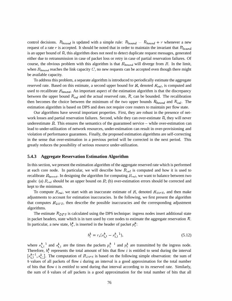
control decisions.���

� ��� is updated with a simple rule:

���� ��� �

� �� ��� � � whenever a new

request of a rate � is accepted. It should be noted that in order to maintain the invariant that� �

� ���

is an upper bound of�

, this algorithm does not need to detect duplicate request messages, generatedeither due to retransmission in case of packet loss or retry in case of partial reservation failures. Ofcourse, the obvious problem with this algorithm is that

� �� ��� will diverge from

�. In the limit,

when� �

� ��� reaches the link capacity � , no new requests can be accepted even though there might

be available capacity.To address this problem, a separate algorithm is introduced to periodically estimate the aggregate

reserved rate. Based on this estimate, a second upper bound for�

, denoted� � � � , is computed and

used to recalibrate���

� ��� . An important aspect of the estimation algorithm is that the discrepancy

between the upper bound� � � � and the actual reserved rate,

�, can be bounded. The recalibration

then becomes the choice between the minimum of the two upper bounds� �

� ��� and

� � � � . Theestimation algorithm is based on DPS and does not require core routers to maintain per flow state.

Our algorithms have several important properties. First, they are robust in the presence of net-work losses and partial reservation failures. Second, while they can over-estimate

�, they will never

underestimate�

. This ensures the semantics of the guaranteed service – while over-estimation canlead to under-utilization of network resources, under-estimation can result in over-provisioning andviolation of performance guarantees. Finally, the proposed estimation algorithms are self-correctingin the sense that over-estimation in a previous period will be corrected in the next period. Thisgreatly reduces the possibility of serious resource under-utilization.

5.4.3 Aggregate Reservation Estimation Algorithm

In this section, we present the estimation algorithm of the aggregate reserved rate which is performedat each core node. In particular, we will describe how

� � � � is computed and how it is used torecalibrate

���� ��� . In designing the algorithm for computing

� � � � , we want to balance between twogoals: (a)

� � � � should be an upper bound on�

; (b) over-estimation errors should be corrected andkept to the minimum.

To compute� � � � , we start with an inaccurate estimate of

�, denoted

� ����� , and then makeadjustments to account for estimation inaccuracies. In the following, we first present the algorithmthat computes

� ����� , then describe the possible inaccuracies and the corresponding adjustmentalgorithms.

The estimate� ����� is calculated using the DPS technique: ingress nodes insert additional state

in packet headers, state which is in turn used by core nodes to estimate the aggregate reservation�

.In particular, a new state,

� �, is inserted in the header of packet � �

:

� �� �

��� �� = � � ��;>=

� = � � (5.12)

where � ��;>=� = and � �

� = are the times the packets � ��;>=

and � �

are transmitted by the ingress node.

Therefore,� �

represents the total amount of bits that flow � is entitled to send during the interval� � ��;>=� =

�� �� = � . The computation of

� ����� is based on the following simple observation: the sum of�

values of all packets of flow � during an interval is a good approximation for the total numberof bits that flow � is entitled to send during that interval according to its reserved rate. Similarly,the sum of

�values of all packets is a good approximation for the total number of bits that all

76

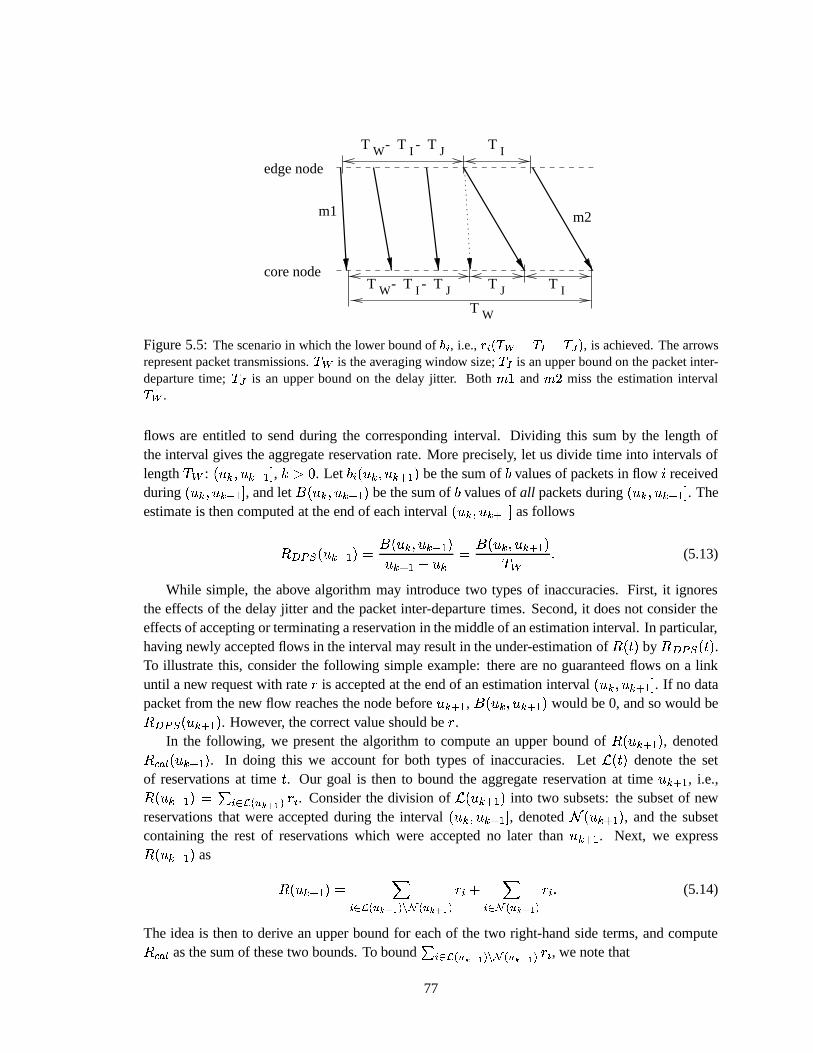
T W

T J T I

T IT JT I --WT

T JT I --WT

edge node

core node

m2m1

Figure 5.5: The scenario in which the lower bound of � � , i.e., � � � � � � � �� � � , is achieved. The arrowsrepresent packet transmissions. ��� is the averaging window size; ��� is an upper bound on the packet inter-departure time; ��� is an upper bound on the delay jitter. Both � and ��� miss the estimation interval��� .

flows are entitled to send during the corresponding interval. Dividing this sum by the length ofthe interval gives the aggregate reservation rate. More precisely, let us divide time into intervals oflength �� : ��� �

� � � � = � , � � �. Let

�

��� �

� � � � = � be the sum of�

values of packets in flow � receivedduring ��� �

� � � � = � , and let � ��� �� � � � = � be the sum of

�values of all packets during ��� �

� � � � = � . Theestimate is then computed at the end of each interval ��� �

� � � � = � as follows

� ����� ��� � � = � � � ��� �� � � � = �

� � � = ��� �� � ��� �

� � � � = � � � (5.13)

While simple, the above algorithm may introduce two types of inaccuracies. First, it ignoresthe effects of the delay jitter and the packet inter-departure times. Second, it does not consider theeffects of accepting or terminating a reservation in the middle of an estimation interval. In particular,having newly accepted flows in the interval may result in the under-estimation of

� � � � by� ����� � � � .

To illustrate this, consider the following simple example: there are no guaranteed flows on a linkuntil a new request with rate � is accepted at the end of an estimation interval ��� �

� � � � = � . If no datapacket from the new flow reaches the node before � � � = , � ��� �

� � � � = � would be 0, and so would be� ����� ��� � � = � . However, the correct value should be � .

In the following, we present the algorithm to compute an upper bound of� ��� � � = � , denoted

� � � � ��� � � = � . In doing this we account for both types of inaccuracies. Let� � � � denote the set

of reservations at time � . Our goal is then to bound the aggregate reservation at time � � � = , i.e.,� ��� � � = � � �

��� � � � � � � �

. Consider the division of

� ��� � � = � into two subsets: the subset of newreservations that were accepted during the interval ��� �

� � � � = � , denoted ��� � � = � , and the subsetcontaining the rest of reservations which were accepted no later than � � � = . Next, we express� ��� � � = � as

� ��� � � = � �

��� � � � � � �� � � � � � � ��

�

� � � � � � � ��

� (5.14)

The idea is then to derive an upper bound for each of the two right-hand side terms, and compute� � � � as the sum of these two bounds. To bound �

��� � � � � � �� � � � � � � � �

, we note that

77

� ��� �� � � � = � �

��� � � � � � �� � � � � � � �

�

��� �

� � � � = � � (5.15)

The reason that (5.15) is an inequality instead of an equality is that when there are flows terminatingduring the interval ��� �

� � � � = � , their packets may still have contributed to � ��� �� � � � = � even though

they do not belong to� ��� � � = ��� ��� � � = � . Next, we compute a lower bound for

�

��� �

� � � � = � . Bydefinition, since ��� � ��� � � = ��� ��� � � = � , it follows that flow � holds a reservation during the entireinterval ��� �

� � � � = � . Let �� be the maximum inter-departure time between two consecutive packetsof a flow at the edge node, and let �� be the maximum delay jitter of a flow. �� represents themaximum difference between the delays experienced by two packets between ingress and egressnodes. The ingress-egress delay of a packet represents the difference between the arrival time of thepacket at the egress node and the departure time of the packet at the ingress node. In the remainderof this section, we assume that � is chosen such that both �� and �� are much smaller than � .Now, consider the scenario shown in Figure 5.5 in which a core node receives the packets

� and� � just outside the estimation window. Assuming the worst case in which

� incurs the lowestpossible delay,

� � incurs the maximum possible delay, and that the last packet before� � departs � seconds earlier, it is easy to see that that the sum of the

�values carried by the packets received

during the estimation interval by the core node cannot be smaller than �

�� � � �� � �� � . Thus, we

have

�

��� �

� � � � = � � �

�� � � ���� �� � � (5.16) ��� � ��� � � = ��� ��� � � = � � (5.17)

By combining Eqs. (5.15) and (5.16), and Eq. (5.13) we obtain

��� � � � � � �� � � � � � � �

�

� ��� � � � � � �� � � � � � � �

�

��� �

� � � � = � � ���� ��

� ����� ��� � � = �����

(5.18)

where �� �� �� � �� � �� � .Next, we bound the second right-hand side term in Eq. (5.14): �

� ��� � � � � � �

For this, we intro-

duce a new global variable��� � .

����� is initialized at the beginning of each interval ��� �

� � � � = � tozero, and is updated to

����� � � every time a new reservation, � , is accepted. Let

��� � � � � denote

the value of this variable at time � . For simplicity, here we assume that a flow which is granted areservation during the interval ��� �

� � � � = � becomes active no later than � � � = .2 Then it is easy to seethat

� � � � � � � �

�

� �

���� ��� � � = � � (5.19)

2Otherwise, to account for the case in which a reservation accepted during the interval �� � � ��� ��� becomes activeafter ��������� , we need to subtract ��������������� �� � � from �� � � � � � � .

78

Per-hop Admission Controlon reservation request �if ( �*"%$'& ��(�� � � � ) � � perform admission test � �� �)��� �/� �)��� � � ;� "%$'& ��( � � "%$'&��)( � � ;accept request;

elsedeny request;

on reservation termination � ��� optional ��� "%$'& ��( � � "%$'&��)( � ;

Aggregate Reservation Bound Comp.on packet arrival �� � � ��+ � � � � ; ��� get b value inserted by ingress (Eq. (5.12)) � �� � � � � ;

on time-out � �� � �� � � � ��� ; ��� estimate aggregate reservation � �� "%$'& ��( � ����� � � "%$'& ��( �'� ���� ��� �� � � �)���5� ;� �)��� � � ;

Figure 5.6: The control path algorithms executed by core nodes; � ����� is initialized to 0.

Eq. (5.19) holds when no duplicate reservation requests are processed, and none of the new acceptedreservations terminate during the interval. Then we define

� � � � ��� � � = � as

� � � � ��� � � = � �� ����� ��� � � = ���� � � � � � ��� � � = � � (5.20)

From Eq. (5.14), and Eqs. (5.18) and (5.19), it follows easily that� � � � ��� � � = � is an upper bound for

� ��� � � = � , i.e.,� � � � ��� � � = � � � ��� � � = � . Finally, we use

� � � � ��� � � = � to recalibrate the upper boundof the aggregate reservation,

���� ��� , at � � � = as

� �� ��� ��� � � = � � �� �� � � � � �

�� ��� � �

� � � � � ��� � � = � � � (5.21)

Figure 5.6 shows the pseudocode of the control algorithms at core nodes. Next we make severalobservations.

First, the estimation algorithm uses only the information in the current interval. This makesthe algorithm robust with respect to loss and duplication of signaling packets since their effectsare “forgotten” after one time interval. As an example, if a node processes both the original anda duplicate of the same reservation request during the interval ��� �

� � � � = � , � � � ��� will be updated

twice for the same flow. However, this erroneous update will not be reflected in the computation of� ����� ��� � � � � , since its computation is based only on the

�values received during ��� � � = � � � � � � .

As a consequence, an important property of our admission control algorithm is that it can asymp-totically reach a link utilization of � � �� � � � � � . In particular, the following property is provenin Appendix B.4:

79

Host 1

Host 2

ingressrouter

egressrouter

100 MbpsHost 3

Host 4

Figure 5.7: The test configuration used in experiments.

Theorem 4 Consider a link of capacity � at time � . Assume that no reservation terminates andthere are no reservation failures or request losses after time � . Then if there is sufficient demandafter � the link utilization approaches asymptotically � � �� � � � � � .

Second, note that since� � � � ��� � � is an upper bound of

� ��� � � , a simple solution would be to use� � � � ��� � � � �

�� � , instead of

� �� ��� , to perform the admission test during ��� �

� � � � = � . The problemwith this approach is that

� � � � can overestimate the aggregate reservation�

. An example is givenin Section 5.5 to illustrate this issue (Figure 5.10(b)).

Third, we note that a possible optimization of the admission control algorithm is to add reser-vation termination messages (see Figure 5.6). This will reduce the discrepancy between the upperbound,

� �� ��� , and the aggregate reservation

�. However, in order to guarantee that

� �� ��� re-

mains an upper bound for�

, we need to ensure that a termination message is sent at most once,i.e., there are no retransmissions if the message is lost. In practice, this property can be enforced byedge nodes, which maintain per flow state.

Finally, to ensure that the maximum inter-departure time is no larger than �� , the ingress nodemay need to send a dummy packet in the case when no data packet arrives for a flow during aninterval �� . This can be achieved by having the ingress node maintain a timer with each flow. Anoptimization would be to aggregate all “micro-flows” between each pair of ingress and egress nodesinto one flow, compute

�values based on the aggregated reservation rate, and insert a dummy packet

only if there is no data packet of the aggregate flow during an interval.

5.5 Experimental Results

We have fully implemented the algorithms described in this chapter in FreeBSD v2.2.6 and deployedthem in a testbed consisting of 266 MHz and 300 MHz Pentium II PCs connected by point-to-point100 Mbps Ethernets. The testbed allows the configuration of a path with up to two core routers. Thedetails of the implementations and of the state encoding are presented in Chapter 8.

In the remainder of this section, we present results from four simple experiments. The ex-periments are designed to illustrate the microscopic behaviors of the algorithms, rather than theirscalability. All experiments were run on the topology shown in Figure 5.7. The first router is con-figured as an ingress node, while the second router is configured as an egress node. An egress nodealso implements the functionalities of a core node. In addition, it restores the initial values of theip off field. All traffic is UDP and all packets are 1000 bytes, not including the header.

In the first experiment we consider a flow between hosts 1 and 3 that has a reservation of 10Mbps but sends at a much higher rate of about 30Mbps. Figures 5.8(a) and (b) plot the arrival anddeparture times for the first 30 packets of the flow at the ingress and egress node, respectively. One

80

0

5

10

15

20

25

30

35

0 5 10 15 20 25

pack

et n

umbe

r

Time (ms)

packet arrivalpacket departure

(a)

0

5

10

15

20

25

30

35

0 5 10 15 20 25

pack

et n

umbe

r

Time (ms)

packet arrivalpacket departure

(b)

Figure 5.8: Packet arrival and departure times for a 10 Mbps flow at (a) the ingress node, and (b) the egressnode.

thing to notice in Figure 5.8(a) is that the arrival rate at the ingress node is almost three times thedeparture rate, which is the same as the reserved rate of 10 Mbps. This illustrate the non workconserving nature of the CJVC algorithm, which enforces the traffic profile and allows only 10Mbps traffic into the network. Another thing to notice is that all packets incur about

� ��� ms delay inthe egress node. This is because they are sent by the ingress node as soon as they become eligible,and therefore � � ����� �

� � � � bits � � Mbps � � ��� � ms. As a result, they will be held in the

rate-controller for this amount of time at the next hop3, which is the egress node in our case.In the second experiment we consider three guaranteed flows between hosts 1 and 3 with reser-

vations of 10 Mbps, 20 Mbps, and 40 Mbps, respectively. In addition, we consider a fourth UDPflow between hosts 2 and 4 which is treated as best effort. The arrival rates of the first three flowsare slightly larger than their reservations, while the arrival rate of the fourth flow is approximately60 Mbps. At time 0, only the best-effort flow is active. At time 2.8 ms, the first three flows be-come simultaneously active. Flows 1 and 2 terminate after sending 12 and 35 packets, respectively.Figure 5.9 shows the packet arrival and departure times for the best-effort flow 4, and the packet de-parture times for the real-time flows 1, 2, and 3. As can be seen, the best-effort packets experiencevery low delay in the initial period of 2.8 ms. After the guaranteed flows become active, best-effortpackets experience longer delays while guaranteed flows receive service at their reserved rate. Afterflow 1 and 2 terminate, the best-effort traffic grabs the remaining bandwidth.

The last two experiments illustrate the algorithms for admission control described in Section 5.4.3.The first experiment demonstrates the accuracy of estimating the aggregate reservation based on the�

values carried in the packet headers. The second experiment illustrates the computation of the ag-gregate reservation bound,

���� ��� , when a new reservation is accepted or a reservation terminates.

In these experiments we use an averaging interval, � , of 5 seconds, and a maximum inter-departuretime, �� , of � � � ms. Because all packets have the same size, the ingress to egress delays experiencedby any two packets of the same flow are practically the same. As a result, we neglect the delay jitter,i.e., we assume �� � �

. This gives us � �� �� � �� � �� � � � � .3Note that since all packets have the same size, � � .

81

0

20

40

60

80

100

120

140

160

180

0 5 10 15 20 25 30

pack

et n

umbe

r

Time (ms)

Flow 1 (packet departure)Flow 2 (packet departure)Flow 3 (packet departure)

Flow 4 (packet arrival)Flow 4 (packet departure)

Figure 5.9: The packets’ arrival and departure times for four flows. The first three flows are guaranteed, withreservations of 10 Mbps, 20 Mbps, and 40 Mbps. The last flow is best effort with an arrival rate of about 60Mbps.

In the first experiment we consider two flows, one with a reservation of 0.5 Mbps, and the otherwith a reservation of 1.5 Mbps. Figure 5.10(a) plots the arrival rate of each flow, as well as thearrival rate of the aggregate traffic. In addition, Figure 5.10(a) plots the bound of the aggregatereservation used by admission test,

���� ��� , the estimate of the aggregate reservation

� ����� , and thebound

� � � � used to recalibrate���

� ��� . According to the pseudocode in Figure 5.6, both

� ����� and� � � � are updated at the end of each estimation interval. More precisely, every 5 seconds

� ����� iscomputed based on the

�values carried in the packet headers, while

� � � � is computed as� ����� � � �

��� ��� � . Note that since, in this case, no new reservation is accepted, we have

��� � � �

,which yields

� � � � �� ����� � � � � . The important thing to note in Figure 5.10(a) is that the rate

variation of the actual traffic (represented by the continuous line) has little effect on the accuracyof computing the aggregate reservation estimate

� ����� , and consequently of� � � � . In contrast,

traditional measurement based admission control algorithms, which base their estimation on theactual traffic, would significantly underestimate the aggregate reservation, especially during thetime periods when no data packets are received. In addition, note that since in this experiment

� � � �is always larger than

���� ��� , and no new reservations are accepted, the value of

� �� ��� is never

updated.In the second experiment we consider a scenario in which a new reservation of 0.5 Mbps is

accepted at time �!� � sec and terminates approximately at time � � ��� sec. For the entire timeduration, plotted in Figure 5.10(b), we have background traffic with an aggregate reservation of0.5 Mbps. Similar to the previous case, we plot the rate of the aggregate traffic, and, in addition,� �

� ��� ,� � � � , and

� ����� . There are several points worth noting. First, when the reservation isaccepted at time � � � sec,

���� ��� increases by the value of the accepted reservation, i.e., 0.5

Mbps (see Figure 5.6). In this way,� �

� ��� is guaranteed to remain an upper bound of the aggregate

reservation�

. In contrast, since both� ����� and

� � � � are updated only at the end of the estimation

82

0

0.2

0.4

0.6

0.8

1

1.2

1.4

1.6

1.8

0 10 20 30 40 50 60

Rat

e (M

bps)

Time (sec)

Flow 1Flow 2

Aggregate Traffic

RDPS

RcalRbound

(a)

0

0.2

0.4

0.6

0.8

1

1.2

1.4

15 20 25 30 35 40 45 50

Rat

e (M

bps)

Time (sec)

Aggregate Traffic

RDPSRcal

Rbound

accept reservation (0.5 Mbps)

terminate reservation (0.5Mbps)

(b)

Figure 5.10: The estimate aggregate reservation � ���! , and the bounds � " $'& ��( and � ���! in the case of (a)two ON-OFF flows with reservations of 0.5 Mbps, and 1.5 Mbps, respectively, and in the case when (b) onereservation of 0.5 Mbps is accepted at time + � -, seconds, and then is terminated at + � .)0 seconds.

Baseline 1 flow 10 flows 100 flowsingress egress ingress egress ingress egress

avg std avg std avg std avg std avg std avg std avg stdenqueue 1.03 0.91 5.02 1.63 4.38 1.55 5.36 1.75 4.60 1.60 5.91 1.81 5.40 2.33dequeue 1.52 1.91 3.14 3.27 2.69 2.81 2.79 3.68 2.30 2.91 2.77 2.82 1.73 2.12

Table 5.4: The average and standard deviation of the enqueue and dequeue times, measured in s.

interval, they underestimate the aggregate reservation, as well as the aggregate traffic, before time�/� � � sec. Second, after

� � � � is updated at time �/� � � sec, as� ����� � � � ��� �

���� , the new

value significantly overestimates the aggregate reservation. This is the main reason for which we donot use

� � � � ( � � � ��� ), but� �

� ��� , to do the admission control test. Third, note that unlike the case

when the reservation was accepted,���

� ��� does not change when the reservation terminates at time

� ����� sec. This is simply because in our implementation no tear-down message is generated whena reservation terminates. However, as

� � � � is updated at the end of the next estimation interval (i.e.,at time �/� � � sec),

���� ��� drops to the correct value of 0.5 Mbps. This shows the importance of

using� � � � to recalibrate

���� ��� . In addition, this illustrates the robustness of our algorithm, i.e.,

the overestimation in a previous period is corrected in the next period. Finally, note that in bothexperiments

� ����� always underestimates the aggregate reservation. This is due to the truncationerrors in computing both the

�values and the

� ����� estimate.

5.5.1 Processing Overhead

To evaluate the overhead of our algorithm we have performed three experiments on a 300 MHzPentium II involving 1, 10, and 100 flows, respectively. The reservation and actual sending rates ofall flows are identical. The aggregate sending rate is about 20% larger than the aggregate reservationrate. Table 5.4 shows the means and the standard deviations for the enqueue and dequeue times at

83

both ingress and egress nodes. Each of these numbers is based on a measurement of 1000 packets.For comparison we also show the enqueue and dequeue times for the unmodified code. There areseveral points worth noting. First, our implementation adds less than 5 � s overhead per enqueueoperation, and about 2 � s per dequeue operation. In addition, both the enqueue and dequeue timesat the ingress node are greater than at the egress node. This is because ingress node performs perflow operations. Furthermore, as the number of flows increases, the enqueue times increase onlyslightly, i.e., by less than 20%. This suggests that our algorithm is indeed scalable in the numberof flows. Finally, the dequeue times actually decrease as the number of flows increases. This isbecause the rate-controller is implemented as a calendar queue with each entry corresponding toa 128 � s time interval. Packets with eligible times falling between the same interval are stored inthe same entry. Therefore, when the number of flows is large, more packets are stored in the samecalendar queue entry. Since all these packets are transferred during one operation when they becomeeligible, the actual overhead per packet decreases.

5.6 Related Work

The idea of implementing guaranteed services by using a stateless core architecture was proposed byJacobson [76] and Clark [24], and is now being pursued by the IETF Diffserv working group [32].There are several differences between our scheme and the existing Diffserv proposals. First, ourDPS based algorithms operate at a much finer granularity both in terms of time and traffic aggre-gates: the state embedded in a packet can be highly dynamic, as it encodes the current state of theflow, rather than the static and global properties such as dropping or scheduling priority. In addition,the goal of our scheme is to implement distributed algorithms that try to approximate the servicesprovided by a network in which all routers implement per flow management. Therefore, we can pro-vide service differentiation and performance guarantees in terms of both delay and bandwidth on aper flow basis. In contrast, the Premium service can provide only per flow bandwidth guarantees.Finally, we propose fully distributed and dynamic algorithms for implementing both data and con-trol functionalities, where existing Diffserv solutions rely on more centralized and static algorithmsfor implementing admission control.

In this chapter, we propose a technique to estimate the aggregate reservation rate and use thatestimate to perform admission control. While this may look similar to measurement-based admis-sion control algorithms [62, 110], the objectives and thus the techniques are quite different. Themeasurement-based admission control algorithms are designed to support controlled-load type ofservices, the estimation is based on the actual amount of traffic transmitted in the past, and is usu-ally an optimistic estimate in the sense that the estimated aggregate rate is smaller than the aggregatereserved rate. While this has the benefit of increasing the network utilization by the controlled-loadservice traffic, it has the risk of incurring transient overloads that may cause the service degradation.In contrast, our algorithm aims to support guaranteed service, and the goal is to estimate a closeupper bound on the aggregate reserved rate even when the the actual arrival rate may vary.

Cruz [29] proposed a novel scheduling algorithm called SCED+ in the context of ATM networks.In SCED+, virtual circuits sharing a same path segment are aggregated into a virtual path. At eachswitch, only per virtual path state instead of per virtual circuit state needs to be maintained forscheduling purpose. In addition, an algorithm is proposed to compute the eligible times and the

84

deadlines of a packet at subsequent nodes when the packet enters a virtual path. We note that bydoing this and using DPS to carry this information in the packets’ headers, it is possible to removeper path scheduling state from core nodes. However, unlike our solution, SCED+ does not provideper flow delay differentiation within an aggregate. In addition, the SCED+ work focuses on the datapath mechanism, while we addresses both data path and control path issues.

5.7 Summary

In this chapter, we have described two distributed algorithms that implement QoS scheduling andadmission control in a SCORE network. Combined, these two algorithms significantly enhancethe scalability of both the data and control planes, while providing guaranteed services with flex-ibility, utilization, and assurance levels similar to those traditionally implemented with per flowmechanisms. The key technique used in both algorithms is Dynamic Packet State (DPS), whichprovides lightweight and robust means for routers to coordinate actions and implement distributedalgorithms. By presenting a design and prototype implementation of the proposed algorithms inIPv4 networks, we have demonstrated that it is indeed possible to apply DPS techniques and haveminimum incompatibility with existing protocols.

85

86

Chapter 6

Providing Relative Service Differentiation in SCORE

In this chapter we describe a third application of the DPS technique: implementing a large spatialgranularity network service, called Location Independent Resource Accounting (LIRA), that pro-vides relative service differentiation. Unlike traditional services, such as the Guaranteed service,that are defined on a per flow basis, large spatial granularity services are defined over a large num-ber of destinations. A simple example would be to guarantee a user 10 Mbps bandwidth irrespectiveof where or when the user sends traffic.

With LIRA, each user is assigned a rate at which it receives resource tokens. For each LIRApacket, a user is charged a number of resource tokens, the amount depending on the congestionlevel along the packet’s path. The goal of LIRA is to achieve both high resource utilization and verylow loss rate. LIRA provides relative differentiation: a user which receives twice as many resourcetokens as another user will receive about twice as much bandwidth, as long as both users share thesame links. Note that in the case of one link, LIRA reduces to Weighted Fair Queueing, i.e., eachactive user is allocated a capacity that is proportional to the rate at which it receives resource tokens.

We present an integrated set of algorithms that implement the LIRA service model in a SCOREnetwork. Specifically, we leverage the existing routing infrastructure to distribute the path costs toall edge nodes. Since the path cost reflects the congestion level along the path, we use this cost todesign dynamic routing and load balancing algorithms. To avoid packet re-ordering within a flow,we devise a lightweight mechanism based on DPS that binds a flow to a route so that all packetsfrom the flow will traverse the same route. To reduce route oscillation, we probabilistically bind aflow to one of the multiple routes.

Traditional solutions to bind a flow to a route, also known as route-pinning, require routers toeither maintain per flow state, or maintain state that is proportional with the square of the numberof edge routers. By using DPS, we are able to significantly reduce this complexity. In particular,we propose a route-pinning mechanism that requires routers to maintain state which is proportionalonly to the number of egress routers.

The rest of the chapter is organized as follows. The next section motivates the LIRA servicemodel, and discusses the limitation of the existing alternatives. Section 6.3 describes the LIRA ser-vice and outlines its implementation in a SCORE network. Section 6.4 presents simulation experi-ments to demonstrate the effectiveness of our solution. Section 6.5 justifies the new service modeland discusses possible ways for our scheme to implement other differential service models. Finally,in Section 6.6 we present the related work, and in Section 6.7 we summarize our contributions.

87

6.1 Background

Traditional service models that propose to enhance the best-effort service are usually defined on aper-flow basis. Examples of such services are the Guaranteed and Controlled Load services [93,121] proposed in the context of Intserv [82], and the Premium service [76] proposed in the contextof Diffserv [32]. While these services provide excellent support for a plethora of new point-to-point applications such as IP telephony and remote diagnostics, there is a growing need to supportservices at a coarser granularity than at a flow granularity. An example would be a service that isdefined irrespective of where or when a user sends its traffic. Such a service would be much easierto negotiate by an organization since there is no need to specify the destinations in advance, usuallya daunting task in practice.1

An example of such a service is the Assured service which was recently proposed by Clark andWroclawski [23, 24] in the context of Diffserv. With the Assured service, a fixed bandwidth profileis associated with each user. This profile describes the commitment of the Internet Service Provider(ISP) to the user. In particular, the user is guaranteed that as long as its aggregate traffic does notexceed its profile, all user’s packets are delivered to their destinations with very high probability.In the remainder of this chapter, we use the term of service assurance to denote the probabilitywith which a packet is delivered to its destination. If a user exceeds its profile, the excess traffic isforwarded as best-effort traffic. Note that the implicit assumption in the Assured service is that thethe traffic sent within a user profile has a much higher assurance (i.e., its packets are delivered witha much higher probability) than the best effort traffic.

In this chapter, we propose a novel service, called Location Independent Resource Accounting(LIRA), in which the service profile is described in terms of resource tokens rather than fixed band-width profile. In particular, with LIRA, each user is assigned a token bucket in which it receivesresource tokens at a fixed rate. When a user sends a packet into the network, the user is charged anumber of resource tokens, the amount depending on the congestion level along the path traversedby the packet. If the user does not have enough resource tokens in its token bucket, the packet isforwarded as a best effort packet. Note that, unlike the Assured service which provides an absoluteservice, LIRA provides a relative service. In particular, if a user receives resource tokens at a ratethat is twice the rate of another user, and if both users sent traffic along the same paths, the first userwill get twice as much aggregate throughput.

A natural question is why use a service that offers only relative bandwidth differentiation suchas LIRA, instead of a service that offers a fixed bandwidth profile such as the Assured service?After all, the Assured service arguably provides a more powerful and useful abstraction; ideally, auser is guaranteed a fixed bandwidth irrespective of where or when it sends traffic. In contrast, withLIRA, the amount of traffic a user can send varies as a result of the congestion along the paths tothe destination.

The simple answer is that, while the fixed bandwidth profile is arguably more powerful, it isunclear whether it can be efficiently implemented. The main problem follows directly from theservice definition, as a fixed bandwidth profile service does not put any restriction on where orwhen a user can send traffic. This results in a fundamental conflict between maximizing resourceutilization and achieving a high service assurance. In particular, since the network does not know in

1For example, for a Web content provider, it is very hard if not impossible to specify its clients a priori.

88

advance where the packets will go, in order to provide high service assurance, it needs to provisionenough resources to all possible destinations. In the worst case, when the traffic of all users traversesthe same congested link in the network, an ISP has to make sure that the sum of all user profilesdoes not exceed the capacity of the bottleneck link. Unfortunately, this will result in severe resourceunderutilization, which is unacceptable in practice. Alternatively, an ISP can provision resources forthe average rather than the worst case scenario. Such a strategy will increase the resource utilizationat the expense of service assurance.

In contrast, LIRA can achieve both high service assurance and resource utilization. However,to achieve this goal, LIRA gives up the fixed bandwidth profile semantics. The bandwidth profileof a user depends on the congestion in the network: the more congested the network, the lowerthe profile of a user. Thus, while the Assured service trades the service assurance for resourceutilization, LIRA trades the fixed bandwidth service semantics for resource utilization. Next, weargue that the trade-off made by LIRA gives a user better control on managing its traffic, whichmakes LIRA a compelling alternative to the Assured service.

To illustrate this point, consider the case when the network becomes congested. In this case,LIRA tries to maintain the level of service assurance by scaling back the profiles of all users thatsend traffic in the congested portion of the network. In contrast, in the case of the Assured service,network congestion will cause a decrease of the service assurance for all users that share the con-gested portion of the network. Consider now a company whose traffic profile decreases from 10to 5 Mbps, as a result of network congestion. Similarly, assume that, in the case of the Assuredservice, the same company experiences a ten fold increase in its loss rate as the result of the networkcongestion (while its service profile remains constant at 10 Mbps). Finally, assume that the CEOof the company wants to make an urgent video conference call, for which requires 2 Mbps. WithLIRA, since the bandwidth required by the video conference is no larger than the company’s trafficprofile, the CEO can initiate the conference immediately. In contrast, with the Assured service, theCEO may not be able to start the conference due to the high loss rate. Worse yet, if the congestion iscaused by the traffic of other users, the company can do nothing about it. The fundamental problemis that, unlike LIRA, the Assured service does not provide any protection in case of congestion.

6.2 Solution Outline

We consider the implementation of LIRA in a SCORE network, in which we use a two bit encodingscheme. The first bit, called the preferred bit, is set by the application or user and indicates thedropping preference of the packet. The second bit, called marking bit, is set by the ingress routersof an ISP and indicates whether the packet is in- or out-of-profile. When a preferred packet arrivesat an ingress node, the node marks it, if the user has not exceeded its profile; otherwise the packetis left unmarked.2 The reason to use two bits instead of one is that in an Internet environment withmultiple ISPs, even if a packet may be out-of-profile in some ISPs on the earlier portion of its path,it may still be in-profile in a subsequent ISP. Having a dropping bit that is unchanged by upstreamISPs on the path will allow downstream ISPs to make the correct decision. Core routers implementa simple behavior of priority-based dropping. Whenever there is a congestion, a core router always

2In this chapter, we will use the terminology of marked or unmarked packets to refer to packets in or out-of the serviceprofile, respectively.

89

drops unmarked packets first. In this chapter, we focus on mechanisms for implementing LIRA ina single ISP. We assume the following model for the interaction of multiple ISPs: if ISP A is usingthe service of ISP B, then ISP B will treat ISP A just like a regular user. In particular, the trafficfrom all ISP A’s users will be treated as a single traffic aggregate.

While the above forwarding scheme can be easily implemented in a Diffserv network, it turnsout that to effectively support LIRA we need the ability to perform route-pinning, that is, to binda flow to a route so that all packets from the flow will traverse the same path. Unfortunately,traditional mechanisms to achieve route pinning require per flow state. Even the recently proposedMulti Protocol Label Switching (MPLS) requires routers to maintain an amount of state proportionalto the square of the number of edge routers. In a large domain with thousands of edge nodes suchoverhead may be unacceptable.

To address this problem we use the Dynamic Packet State (DPS) technique. With each packetwe associate a label that encodes the packet’s route from the current node to the egress router. Packetlabels are initialized by ingress routers, and are used by core routers to route the packets. When apacket is forwarded, the router updates its label to reflect the fact that the remaining path has beenreduced by one hop. By using this scheme, we are able to significantly reduce the state maintainedby core routers. More precisely, this state becomes proportional to the number of egress nodesreachable from the core router, which can be shown to be optimal. The route pinning mechanism isdescribed in detail in Section 6.3.4.

6.3 LIRA: Service Differentiation based on Resource Right Tokens

In this section, we present our differential service model, called LIRA (Location Independent Re-source Accounting), with service profiles defined in terms of resource tokens rather than absoluteamounts of bandwidth.

With LIRA, each user � is assigned a service profile that is characterized by a resource tokenbucket � �

� �� , where �

represents the resource token rate, and

�

represents the depth of the bucket.

Unlike traditional token buckets where each preferred bit entering the network consumes exactlyone token, with resource token buckets the number of tokens needed to admit a preferred bit is adynamic function of the path it traverses.

Although there are many functions that can be used, we consider a simple case in which eachlink � is assigned a cost, denoted �

� � � , which represents the amount of resource tokens charged for

sending a marked bit along the link at time � . The cost of sending a marked packet is computed as�� � �

��

� � � , where � is the packet length and

�is the set of links traversed by the packet. While

we focus on unicast communications in this chapter, we note that the cost function is also naturallyapplicable to the case of multicast. As we will show in Section 6.4, charging a user for every linkit uses and using the cost in routing decisions helps to increase the network throughput. In fact, ithas been shown by Ma et al. [68] that using a similar cost function3 for performing the shortest pathrouting gives the best overall results when compared with other dynamic routing algorithms.

It is important to note that the costs used here are not monetary in nature. Instead they arereflecting the level of congestion and the resource usage along links/paths. This is different from a

3It can be shown that when all links have the same capacity our cost is within a constant factor from the cost ofshortest-dist(P, 1) algorithm proposed by Ma et al. [68].

90

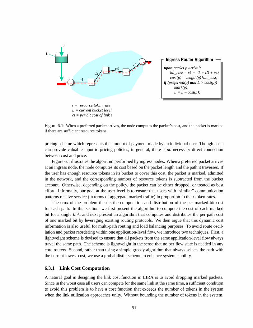
r

r = resource token rateL = current bucket levelci = per bit cost of link i

Ingress Router Algorithm

upon packet p arr ival:bit_cost = c1 + c2 + c3 + c4;cost(p) = length(p)*bit_cost;

if (preferred(p) and L > cost(p))mark(p);L = L – cost(p);

L

c1

c2c3

c4

Figure 6.1: When a preferred packet arrives, the node computes the packet’s cost, and the packet is markedif there are sufficient resource tokens.

pricing scheme which represents the amount of payment made by an individual user. Though costscan provide valuable input to pricing policies, in general, there is no necessary direct connectionbetween cost and price.

Figure 6.1 illustrates the algorithm performed by ingress nodes. When a preferred packet arrivesat an ingress node, the node computes its cost based on the packet length and the path it traverses. Ifthe user has enough resource tokens in its bucket to cover this cost, the packet is marked, admittedin the network, and the corresponding number of resource tokens is subtracted from the bucketaccount. Otherwise, depending on the policy, the packet can be either dropped, or treated as besteffort. Informally, our goal at the user level is to ensure that users with “similar” communicationpatterns receive service (in terms of aggregate marked traffic) in proportion to their token rates.

The crux of the problem then is the computation and distribution of the per marked bit costfor each path. In this section, we first present the algorithm to compute the cost of each markedbit for a single link, and next present an algorithm that computes and distributes the per-path costof one marked bit by leveraging existing routing protocols. We then argue that this dynamic costinformation is also useful for multi-path routing and load balancing purposes. To avoid route oscil-lation and packet reordering within one application-level flow, we introduce two techniques. First, alightweight scheme is devised to ensure that all packets from the same application-level flow alwaystravel the same path. The scheme is lightweight in the sense that no per flow state is needed in anycore routers. Second, rather than using a simple greedy algorithm that always selects the path withthe current lowest cost, we use a probabilistic scheme to enhance system stability.

6.3.1 Link Cost Computation

A natural goal in designing the link cost function in LIRA is to avoid dropping marked packets.Since in the worst case all users can compete for the same link at the same time, a sufficient conditionto avoid this problem is to have a cost function that exceeds the number of tokens in the systemwhen the link utilization approaches unity. Without bounding the number of tokens in the system,

91

this suggests a cost function that goes to infinity when the link utilization approaches unity. Amongmany possible cost functions that exhibit this property, we choose the following one:

� � � � � ��� � � � �

�(6.1)

where � is the fixed cost of using the link4 when it is idle, and � � � � represents the link utilization attime � . In particular, � � � � � � � � � � � , were

� � � � is the traffic throughput at time � , and � representsthe link capacity. Recall that ��� � � is measured in tokens/bit and represents how much a user ischarged for sending a marked bit along that link at time � .

In an ideal system, where costs are instantaneously distributed and the rate of the incomingtraffic varies slowly, a cost function as defined by Eq. (6.1) guarantees that no marked packets aredropped inside the core. However, in a real system, computing and distributing the cost informationincur overhead, so they are usually done periodically. In addition, there is always the issue ofpropagation delay. Because of these, the cost information used in admitting packets at ingress nodesmay be obsolete. This may cause packet dropping, and lead to oscillations. Though oscillationsare inherent to any system in which the propagation of the feed-back information is non-zero, thesensitivity of our cost function when the link utilization approaches unity makes things worse. Inthis regime, an incrementally small traffic change may result in an arbitrary large cost change. Infact one may note that Eq. (6.1) is similar to the equation describing the delay behavior in queueingsystems [65], which is known to lead to system instability when used as a congestion indication ina heavily loaded system.

To address these issues, we use the following iterative formula to compute the link cost:

� � �� � � � ��� �

;>= �

�� � �� �;>= �� � (6.2)

where �� � � � � � denotes the average bit rate of the marked traffic during the time interval � � � � � . Itis easy to see that if the marked traffic rate is constant and equal to

�, the above iteration converges

to the cost given by Eq. (6.1). The main advantage of using Eq. (6.2) over Eq. (6.1) is that it ismore robust against large variations in the link utilization. In particular, when the link utilizationapproaches unity the cost increases by at most � every iteration. In addition, unlike Eq. (6.1),Eq. (6.2) is well defined even when the link is congested, i.e., �� � � ;>= � �

� � � .

Unfortunately, computing the cost by using Eq. (6.2) is not as accurate as by using Eq. (6.1).The link may become and remain congested for a long time before the cost increase is large enoughto reduce the arrival rate of marked bits. This may result in the loss of marked packets, which wetry to avoid. To alleviate this problem we use only a fraction of the link capacity,

�� �

�� , for the

marked traffic, the remaining being used to absorb the unexpected variations due to inaccuracies inthe cost estimation.5 Here, we chose

�between 0.85 and 0.9.

6.3.2 Path Cost Computation and Distribution

In LIRA, the cost of a marked bit over a path is the sum of the costs of a marked bit over each linkon the path. Once the cost for each link is computed, it is easy to compute and distribute the path

4In practice, the network administrator can make use of � to encourage/discourage the use of the link. Simply bychanging the fixed cost � , a link will cost proportionally more or less at the same utilization.

5 � is similar to the pressure factor used in some ABR congestion control schemes for estimating the fair share [61, 87].

92

532 ididid��

1id

75id

DST COST LABEL

542 ididid��

8

532 ididid��

5id

DSTLABEL

542 ididid ��

ROUTING TABLE

NEXT HOP

5id

2id

2id

FORWARDING TABLE

53 idid�

5id

DSTLABEL

54 idid�

NEXT HOP

5id

3id

4id

FORWARDING TABLE

5id 5id

DSTLABEL NEXT HOP

5id

FORWARDING TABLE

532 ididlabelidlabel����

532 idididlabel���

3

33

1

22id

3id

4id

5id

53 idlabelidlabel ���

Figure 6.2: Example of route binding via packet labeling.

cost by leveraging existing routing protocols. For link state algorithms, the cost of each marked bitcan be included as part of the link state. For distance vector algorithms, we can pass and computethe partial path cost in the same way the distance of a partial path is computed with respect to therouting metric.

6.3.3 Multipath Routing and Load Balancing

Since our algorithm defines a dynamic cost function that reflects the congestion level of each link,it is natural to use this cost function for the purpose of multi-path routing. To achieve this, wecompute the

�shortest paths for each destination or egress node using the unit link metric. While

the obvious solution is to send packets along the path with the minimum cost (in the sense of LIRA,see Section 6.3) among the

�paths, this may introduce two problems: (a) packet re-ordering within

one application-level flow, which may negatively affect end-to-end congestion control algorithms,and (b) route oscillation, which may lead to system instability.

We introduce two techniques to address these problems. First, we present a lightweight mech-anism that binds a flow to a route so that all packets from the flow will traverse the same route.Second, to reduce route oscillation, for each new flow, an ingress node probabilistically binds it toone of the multiple routes. By carefully selecting the probability, we can achieve both stability andload-balancing.

6.3.4 Route Pinning

As discussed earlier, we will maintain multiple routes for each destination. However, we wouldlike to ensure that all packets belonging to the same flow are forwarded along the same path. To

93

implement this mechanism we use the Dynamic Packet State (DPS) technique.The basic idea is to associate with each path a label computed as the XOR over the identifiers of

all routers along the path, and then associate this label with each packet of a flow that goes along thatpath. Here we use the IP address as the identifier. More precisely, a path

� � � � � � � � � = � � � � � � ��� ,

where � ��� is the source and � � � is the destination, is encoded at the source ( � � � ) by � � � � � = �� � � � � � � � � � � . Similarly, the path from � � = to � � � is encoded at � � = by � = � � � � � � � � � � � � . Apacket that travels along path

�is labeled with � � as it is leaving � � � , and with � = as it is leaving

�= .

By using XOR we can iteratively re-compute the label based on the packet’s current label and thenode identifier. As an example, consider a packet that is assigned label � � at node � � � . When thepacket arrives at node � � = , the new label corresponding to the remaining of the path, � � � = � � � � � � �

�� ,

is computed as follows:

� = � � � = � � � � (6.3)� � = � � � � = � � � � � � � � � � � � � ��� � � � � � � � � � � �It is easy to see that this scheme guarantees that the packet will be forwarded exactly along the path

�. Here, we implicitly assume that all alternate paths between two end-nodes have unique labels.

Although theoretically there is a non-zero probability that two labels may collide, we believe thatfor practical purposes it can be neglected. One possible way to reduce the label collision probabilitywould be to use a hash function to translate the IP addresses into labels. By using a good hashfunction, this will result in a more random distribution of router labels. Another possibility wouldbe to explicitly label routers to reduce or even eliminate the collision probability. Note that thissolution will require to maintain the mapping between router IP addresses and router labels, whichcan be difficult in practice. One last point worth noting is that even if two alternate paths have thesame label, this will not jeopardize the correctness of our scheme: the worst thing that can happenis an alternate path to be ignored, which will only lead to a decrease in utilization.

Next we give some details of how this mechanism can be implemented by simply extending theinformation maintained by each router in the routing and forwarding tables. Besides the destinationand the route cost, each entry in the routing table also contains the label associated with that path.�

���� �

�� ���

�=� � � � = � � � � � �

�� ���

��� � � � � � � ��� (6.4)

Similarly, the forwarding table should contain an entry for each path:�� � = � � � ��� � �:' ��� �� � � = � � � � �

�� � � � � � ��� � �:' ��� �� � � � � � (6.5)

In Figure 6.2 we give a simple example to illustrate this mechanism. Assume that nodes � � = and� � � are edge nodes, and there are two possible paths from � � = to � � � of costs 7, and 8, respectively.Now, assume a packet destined to � � � arrives at � � = . First the ingress node � � = searches the classifiertable (not shown in the Figure) that maintains a list of all flows to see whether this is the first packetof a flow. If it is, the router uses the information in the routing table to probabilistically bind theflow to a path to � � � . At the same time it labels the packet with the encoding of the selected route.In our example, assume the path of cost 7, i.e., � � � = � � � � � � � � � � � � , is selected. If the arriving packetis not the first packet of the flow, the router automatically labels the packet with the encoding of thepath to which the flow is bound. This can be simply achieved by keeping a copy of the label in the

94

classifier table. Once the packet is labeled, the router checks the forwarding table for the next hopby matching the packet’s label and its destination. In our case, this operation gives us � � � as the nexthop. When the packet arrives at node � � � the router first computes a new label based on the currentpacket label and the router identifier: � � � '�� ��� � � � � � � '�� . The new label is then used to lookup theforwarding table.

It is important to note that the above algorithm assumes per flow state only at ingress nodes.Inside the core, there is no per flow state. Moreover, the labels can speed-up the table lookup if usedas hash keys.

6.3.5 Path Selection

While the above forwarding algorithm ensures that all packets belonging to the same flow traversethe same path, there is still the issue of how to select a path for a new flow. The biggest concernwith any dynamic routing protocol based on congestion information is its stability. Frequent routechanges may lead to oscillations.

To address this problem, we associate a probability with each route and use it in binding a newflow to that route. The goal in computing this probability is to equalize the costs along the alternateroutes, if possible. For this we use a greedy algorithm. Every time the route costs are updatedwe split the set of routes in two equal sets, where all the routes in one set have costs larger thanthe routes in the second set. If there is an odd number of routes, we leave the median out. Then,we decrease the probability of every route in the first set, the one which contains the higher costroutes, and increase the probability of each route in the second set by a small constant � . It can beshown that in a steady-state system, this algorithm converges to the desired solution, in which thedifference between the costs of the two alternate paths is bounded by � .

6.3.6 Scalability

As described so far, it is required that our scheme maintains�

entries for each destination in both theforwarding table used by the forwarding engine and the routing table used by the routing protocol,where

�is the maximum number of alternate paths. While this factor may not be significant if

�

is small, a more serious issue that potentially limits the scalability of the algorithm is that in itsbasic form it requires that an entry be maintained for each destination, where in reality, to achievescalability, routers really maintain the longest-prefix of a group of destinations that share the sameroute [41]. Since our algorithm works in the context of one ISP, we can maintain an entry for eachegress node instead of each destination. We believe this is sufficient as the number of egress nodesin an ISP is usually not large.

However, assume that the number of egress nodes in an ISP is very large so that significantaddress aggregation is needed. Then we need to also perform cost aggregation. To illustrate theproblem consider the example in Figure 6.3. Assume the addresses of

� �and

�= are aggregated

at an intermediate router � = . Now the question is how much to charge a packet that enters at theingress node �

�and has the destination

���. Since we do not keep state for the individual routes

to� �

, and�= respectively, we need to aggregate the cost to these two destinations. In doing this,

a natural goal would be to maintain the total charges the same as in a reference system that keepsper route state. Let

� � � =� �� denote the average traffic rate from � = to

�, � � � � . Then, in the

95

r0 r1

d0

d1

Figure 6.3: Topology to illustrate the label and cost aggregation.

reference system that maintains per route state, the total charge per time unit for the aggregate trafficfrom � = to

� �and

�= is: � ��� � � =

� � � � � � � =� ��� � � � ��� � � =

� �= �� � � =

� �= � . In a system that does not

maintain per route state, the charge for the same traffic is � ��� � � =� � � � �

= � �� � � =

� ��� � � � � � =� �= � � ,

where � ��� � � =� ��� � �

= � denotes the per bit aggregate cost. This yields

� ��� � � =� � � � �

= � � � ��� � � =� ��� � � � � =

� � � �� � � =

� ��� � � � � � =� �= �� (6.6)

� ��� � � =� �= �� � � =

� �= �� � � =

� � � � � � � � =� �= ��

Thus, any packet that arrives at ��

and has either destination� �

or�= is charged with � ��� � � � � � = � �

� ��� � � =� ��� � �

= � . Obviously, route aggregation increases the inaccuracies in cost estimation. How-ever, this may be alleviated by the fact that the route aggregation usually exhibits high localities.

Another problem with address aggregation is that a label can no longer be used to encode theentire path to the destination. Instead, it is used to encode the common portion of the paths to thedestinations in the aggregate set. This means that a packet should be relabeled at every router thatperforms aggregation involving the packet’s destination. The most serious concern with this schemeis that it is necessary to maintain per flow state and perform packet classification at a core router ( � =in our example). Fortunately, this scalability problem is alleviated by the fact that we need to keepper flow state only for the flows whose destination addresses are aggregated at the current router.Finally, we note that this problem is not specific to our scheme; any scheme that (i) allows multiplepath routing, (ii) performs load balancing, and (iii) avoids packet reordering has to address it.

6.4 Simulation Results

In this section we evaluate our model by simulation. We conduct four experiments: three involvingsimple topologies which help to gain a better understanding of the behavior of our algorithms, andone more realistic example with a larger topology and more complex traffic patterns. The firstexperiment shows that if all users share the same congested path, then each user receives servicein proportion to its resource token rate. This is the same result one would expect from using aweighted fair queueing scheduler on every link, with the weights set to the users’ token rate. Inthe second experiment, we show that by using dynamic routing and load balancing, we are able toachieve the same result – that is, each user receives service in proportion to its token rate – in amore general configuration where simply using weighted fair queueing scheduler on every link isnot sufficient. In the third experiment, we show how load balancing can significantly increase the

96

overall resource utilization. Finally, the fourth experiment shows how the behaviors observed in theprevious experiments scale to a larger topology.

6.4.1 Experiment Design

We have implemented a packet level simulator which supports both Distance Vector (DV) and Short-est Path First (SPF) routing algorithms. To support load balancing we extended these algorithms tocompute the

�-th shortest paths. The time interval between two route updates is uniformly dis-

tributed between� ��� and ���� of the average value. As shown by Floyd and Jacobson [38], this

choice avoids the route-update self-synchronization. In SPF, when a node receives a routing mes-sage, it first updates its routing table and then forwards the message to all its neighbors, except thesender. The routing messages are assumed to have high priority, so they are never lost. In the nextsections we compare the following schemes:

� BASE – this scheme models today’s best-effort Internet, and it is used as a baseline in ourcomparison. The routing protocol uses the number of hops as the distance metric and it isimplemented by either DV or SPF. This scheme does not implement service differentiation,i.e., both marked and unmarked packets are identically treated.

� STATIC – this scheme implements the same static routing as BASE. In addition, it implementsLIRA by computing the link cost as described in Section 6.3.1, and marking packets at eachingress node according to the algorithm shown in Figure 6.1.

� DYNAMIC-�

– this scheme adds dynamic routing and load balancing to STATIC. The rout-ing protocol uses a modified version of DV/SPF to find the first

�shortest paths. Note that

DYNAMIC-1 is equivalent to STATIC.

Each router implements a FIFO scheduling discipline with a shared buffer and a drop-tail man-agement scheme. When the buffer occupancy exceeds a predefined threshold, newly arrived un-marked packets are dropped. Thus, the entire buffer space from the threshold up to its total size isreserved to the in-profile traffic.6 Unless otherwise specified, throughout all our experiments we usea buffer size of 256 KB and a threshold of 64 KB.

The two main performance indices that we use in comparing the above schemes are the userin-profile and user overall throughputs. The user in-profile throughput represents the rate of the useraggregate in-profile traffic delivered to its destinations. The overall throughput represents the user’sentire traffic — i.e., including both the in- and out-of profile traffic — delivered to its destinations.In addition, we use user dropping rate of the in-profile traffic to characterize the level of serviceassurance.

Recent studies have shown that the traffic in real networks exhibits the self-similar property [27,80, 81, 118] — that is, the traffic is bursty over widely different time scales. To generate self-similar traffic we use the technique originally proposed by Willinger et al. [118], where it was

6We note that this scheme is a simplified version of the RIO buffer management scheme proposed by Clark andWroclawski [24] In addition, RIO implements a Random Early Detection (RED) [37] dropping policy, instead of drop-tail, for both in- and out-of profile traffic. RED provides an efficient detection mechanism for the adaptive flows, such asTCP, allowing them to gracefully degrade their performances when congestion occurs. However, since in this study weare not concerned with the behavior of individual flows, for simplicity we chose to not implement RED.

97

link 2 link 3

link 1 link 6link 5S1S1 D1D1

S2S2 S3S3

link 4

(a)��������

������������ ������������

������������������������������������������

������������������������������������������

4.38

2.78

3.88

3.05 3.06

Thr

ough

put (

Mbp

s)S1 S2 S3 S1 S2 S3

BASE

2.83

STATIC

best-effort in-profile

������������

������������

out-of profile

������������������������������������������������������������

������������������������������������������������������������

(b)

in-profile out-of profile

� � � � � � � � � �

������������������������������

�����������������������������������������������������������������������������������������������

�����������������������������������������������������������������������������������������������

������������������������������������������������������������

������������������������������������������������������������

S1 S2 S3

4.40

2.45

3.13

Thr

ough

put (

Mbp

s)

��������

STATIC

����

(c)

Figure 6.4: (a) Topology used in the first experiment. Each link has 10 Mbps capacity. 1 , 13� , and 15. sendall their traffic to 4 . (b) The throughputs of the three users under BASE and STATIC schemes. (c) Thethroughputs under STATIC when the token rate of 12� is twice the rate of 1 / 13� .

shown that the superposition of many ON-OFF flows with ON and OFF periods drawn from a heavytail distribution, and which have fixed rates during the ON period results in self-similar traffic. Inparticular, Willinger et al. [118] show that the aggregation of several hundred of ON-OFF flows is areasonable approximation of the real end-to-end traffic observed in a LAN.

In all our experiments, we generate the traffic by drawing the length of the ON and OFF periodsfrom a Pareto distribution with the power factor of �� � . During the ON period a source sends packetswith sizes between 100 and 1000 bytes. The time to send a packet of minimum size during the ONperiod is assumed to be the time unit in computing the length of the ON and OFF intervals.

Due to the high overhead incurred by a packet-level simulator such as ours, we limit the linkcapacities to 10 Mbps and the simulation time to 200 sec. We set the average interval betweenrouting updates to 5 sec for the small topologies used in the first three experiments, and to 3 sec forthe large topology used in the last experiment. In all experiments, the traffic starts at time � � � �sec. The choice of this time guarantees that the routing algorithm finds at least one path betweenany two nodes by time � . In order to eliminate the transient behavior, we start our measurements attime � � � � sec.

6.4.2 Experiment 1: Local Fairness and Service Differentiation

This experiment shows that if all users send their traffic along the same congested path, they getservice in proportion to their token rate, as long as there is enough demand. Consider the topologyin Figure 6.4(a), where users � , � � , and � � send traffic to

� . Figure 6.4(b) shows the user overallthroughputs over the entire simulation under BASE. As it can be seen, � gets significantly morethan the other two. In fact, if the traffic from all sources were continuously backlogged, we expectthat � will get half of the congested links � and � , while � � and � � split the other half. Thisis because even though each user sends at an average rate higher than 10 Mbs, the queues are notcontinuously backlogged. This is due to the bursty nature of the traffic and due to the limited bufferspace at each router.

98

link 1

link 3S3S3 D1D1

S4S4

link 2

S2S2

S1S1

D2D2

D3D3

(a)S2 S3 S4 S1 S2 S3 S4 S1 S2 S3 S4S1

DYNAMIC-2

3.25 3.213.52

8.74

3.32 3.32 3.35

8.74

4.89 4.90 4.965.22

��������

��������

in-profile

������������������������������������������������������������������������������������������������������

������������������������������������������������������������������������������������������������������

����������������������������������������������������������������������

����������������������������������������������������������������������

����������������������������

��������������

���������������������������������������

���������������������������������������

� � � � � � � � � � � � � � � � � � � �

������������������������������������������������������������

BASE STATIC

out-of profile

����������������������������������������������������������������������������������������������������

������������������������������������������������������������

Thr

ough

put (

Mbp

s)

����������������������������������������������������������������������������������������������������

����������������������������������������������������������������������������������������������������

best-effort

���������������������������������������������������������������������������������������������������������

���������������������������������������������������������������������������������������������������������

��������

(b)

Figure 6.5: (a) Topology used in the second experiment. 1 , 13� , 15. , and 1 � send all their traffic to 4 ,46� , and 46. , respectively. (b) The throughputs of all users under BASE, STATIC, and DYNAMIC-2.

Next, we run the same simulation for the STATIC scheme. To each user we assign the sametoken rate, and to each link we associate the same fixed cost. Figure 6.4(b) shows the user overalland in-profile throughputs. Compared to BASE, the overall throughputs are more evenly distributed.However, the user � still gets slightly better service, i.e., its in-profile throughput is 3.12 Mbps,while the in-profile throughput of � � / � � is 2.75 Mbps. To see why, recall from Eq. (6.1) that linkcost accurately reflects the level of congestion on that link. Consequently, in this case links 5 and 6will have the highest cost, followed by link 4, and then the other three links. Thus, � � and � � haveto “pay” more than � per marked bit. Since all users have the same token rates, this translates intolower overall throughputs for � � and � � , respectively.

To illustrate the relationship between the user’s token rate and its performance, we double thetoken rate of � � . Figure 6.4(c) shows the overall and in-profile throughputs of each user. In terms ofin-profile traffic, user � � gets roughly twice the throughout of � � (i.e., 4.27 Mbps vs. 2.18 Mbps).

Finally, we note that there were no marked packets dropped in any of the above simulations. Forcomparison, more than 60% of the out-of profile traffic was dropped.

6.4.3 Experiment 2: User Fairness and Load Balancing

In this section we show how dynamic routing and load balancing help to improve user level fairnessand achieve better resource utilization. Consider the topology in Figure 6.5 where users � , � � , � �and � � send traffic to each of the users

� , � � and� � , respectively. Again the fixed costs of all

links are equal, and all users are assigned the same token rate.Figure 6.5(b) shows the overall and in-profile throughputs of � , � � , � � and � � under BASE,

STATIC and DYNAMIC-2, respectively. When BASE and STATIC are used, each user always sendsalong the shortest paths. This results in � , � � and � � sharing link 1, while � � alone uses link 3. Asa consequence � � receives significantly better service than the other three users. Since it implementsthe same routing algorithm, STATIC does not improve the overall throughputs. However, compared

99

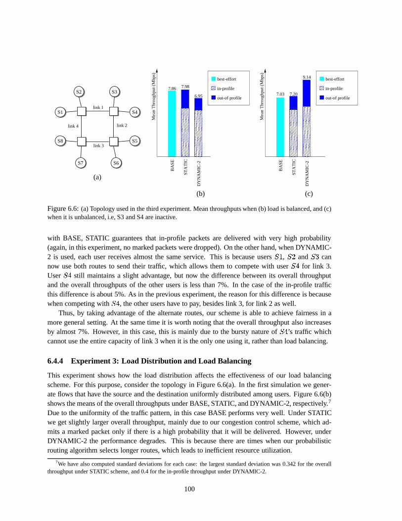
link 1

S2S2

link 4

S8S8 S5S5

S1S1

S7S7 S6S6

S4S4

S3S3

link 2

link 3

(a)B

ASE

DY

NA

MIC

-2

6.95

7.987.86

STA

TIC

������������

Mea

n T

hrou

ghpu

t (M

bps)

���������

���������

������������

best-effort

in-profile

out-of profile

��������������������������������������������������������������������������������

������������������������������������������������

����������������������������������

����������������������������������

(b)

9.14

BA

SE

DY

NA

MIC

-2

7.03 7.20

STA

TIC

Mea

n T

hrou

ghpu

t (M

bps)

��������������������������������������������������������������������������������

������������������������������������������������

� � �

���������

������������

best-effort

in-profile

out-of profile

������������������������������������������������������

������������������������������������������������������

������������

(c)

Figure 6.6: (a) Topology used in the third experiment. Mean throughputs when (b) load is balanced, and (c)when it is unbalanced, i.e, S3 and S4 are inactive.

with BASE, STATIC guarantees that in-profile packets are delivered with very high probability(again, in this experiment, no marked packets were dropped). On the other hand, when DYNAMIC-2 is used, each user receives almost the same service. This is because users � , � � and � � cannow use both routes to send their traffic, which allows them to compete with user � � for link 3.User � � still maintains a slight advantage, but now the difference between its overall throughputand the overall throughputs of the other users is less than 7%. In the case of the in-profile trafficthis difference is about 5%. As in the previous experiment, the reason for this difference is becausewhen competing with � � , the other users have to pay, besides link 3, for link 2 as well.

Thus, by taking advantage of the alternate routes, our scheme is able to achieve fairness in amore general setting. At the same time it is worth noting that the overall throughput also increasesby almost 7%. However, in this case, this is mainly due to the bursty nature of � � ’s traffic whichcannot use the entire capacity of link 3 when it is the only one using it, rather than load balancing.

6.4.4 Experiment 3: Load Distribution and Load Balancing

This experiment shows how the load distribution affects the effectiveness of our load balancingscheme. For this purpose, consider the topology in Figure 6.6(a). In the first simulation we gener-ate flows that have the source and the destination uniformly distributed among users. Figure 6.6(b)shows the means of the overall throughputs under BASE, STATIC, and DYNAMIC-2, respectively.7

Due to the uniformity of the traffic pattern, in this case BASE performs very well. Under STATICwe get slightly larger overall throughput, mainly due to our congestion control scheme, which ad-mits a marked packet only if there is a high probability that it will be delivered. However, underDYNAMIC-2 the performance degrades. This is because there are times when our probabilisticrouting algorithm selects longer routes, which leads to inefficient resource utilization.

7We have also computed standard deviations for each case: the largest standard deviation was 0.342 for the overallthroughput under STATIC scheme, and 0.4 for the in-profile throughput under DYNAMIC-2.

100

S13S13

N1N1

N2N2 N3N3 N4N4

N5N5

N6N6N8N8

N9N9N10N10

N11N11

S12S12 S11S11

S19S19

S18S18

S17S17

S10S10

S9S9S8S8S7S7S6S6S5S5S4S4

S3S3

S2S2

S1S1

S14S14

S15S15S16S16

N7

(b)

(c)

(a)

Figure 6.7: Topology similar to the T3 topology of the NSFNET backbone network containing the IBMNSS nodes.

Next, we consider an unbalanced load by making users � � and � � inactive. Figure 6.6(c) showsthroughput means under BASE, STATIC, and DYNAMIC-2, respectively. As it can be noticed,using DYNAMIC-2 increases the mean by 30%. This is because under BASE and STATIC schemesthe entire traffic between � , � � and � � , � � is routed through links 3 and 4 only. On the other hand,DYNAMIC-2 takes advantage of the alternate route through links 1 and 2.

Finally, in another simulation not shown here we considered the scenario in which � � , � � , � � ,and � � send their entire traffic to � � and � � , respectively. In this case DYNAMIC-2 outperformsSTATIC and BASE by almost two times in terms of in-profile and overall throughputs. This is againbecause BASE and STATIC exclusively use links 3 and 2, while DYNAMIC-2 is able to use all fourlinks.

6.4.5 Experiment 4: Large Scale Example

In this section we consider a larger topology that closely resembles the T3 topology of the NSFNETbackbone containing the IBM NSS nodes (see Figure 6.7). The major difference is that in order tolimit the simulation time we assume 10 Mbps links, instead of 45 Mbps. We consider the followingthree scenarios.

101

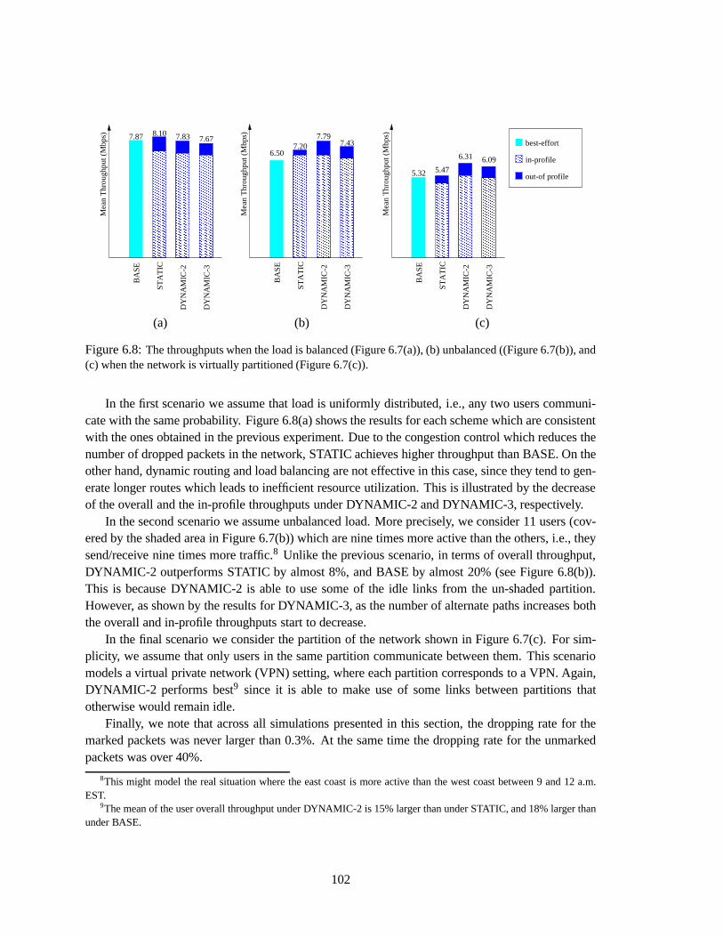
DY

NA

MIC

-3

7.87 8.10 7.83 7.67

DY

NA

MIC

-2

BA

SE

Mea

n T

hrou

ghpu

t (M

bps)

������������������������������������������������������������

������������������������������������������������������������

����������������������������������������������������������������������������������������������������

������������������������������������������������������������

STA

TIC

������������������������������������������������������������

������������������������������������������������������������

(a)

DY

NA

MIC

-3

6.507.20

7.797.43

DY

NA

MIC

-2

BA

SE

Mea

n T

hrou

ghpu

t (M

bps)

������������������������������������������������������������

������������������������������������������������������������

��������������������

��������������������

��������������������������

��������������������������

STA

TIC

� � � � � � � � � � � � � � � � � � � � � � � � � � � � � � � � � � � � � � � �

������������������������������������������������������������

(b)

BA

SE

DY

NA

MIC

-3

5.32 5.47

6.31 6.09

DY

NA

MIC

-2

������������������������������������������

������������������������������������������

Mea

n T

hrou

ghpu

t (M

bps)

��������������������������������������������������������������������������������

��������������������������������������������������������������������������������

������������������������������������������������

������������������������������������������������

��������������������������

������������

���������

���������

������������

STA

TIC

best-effort

in-profile

out-of profile

(c)

Figure 6.8: The throughputs when the load is balanced (Figure 6.7(a)), (b) unbalanced ((Figure 6.7(b)), and(c) when the network is virtually partitioned (Figure 6.7(c)).

In the first scenario we assume that load is uniformly distributed, i.e., any two users communi-cate with the same probability. Figure 6.8(a) shows the results for each scheme which are consistentwith the ones obtained in the previous experiment. Due to the congestion control which reduces thenumber of dropped packets in the network, STATIC achieves higher throughput than BASE. On theother hand, dynamic routing and load balancing are not effective in this case, since they tend to gen-erate longer routes which leads to inefficient resource utilization. This is illustrated by the decreaseof the overall and the in-profile throughputs under DYNAMIC-2 and DYNAMIC-3, respectively.

In the second scenario we assume unbalanced load. More precisely, we consider 11 users (cov-ered by the shaded area in Figure 6.7(b)) which are nine times more active than the others, i.e., theysend/receive nine times more traffic.8 Unlike the previous scenario, in terms of overall throughput,DYNAMIC-2 outperforms STATIC by almost 8%, and BASE by almost 20% (see Figure 6.8(b)).This is because DYNAMIC-2 is able to use some of the idle links from the un-shaded partition.However, as shown by the results for DYNAMIC-3, as the number of alternate paths increases boththe overall and in-profile throughputs start to decrease.

In the final scenario we consider the partition of the network shown in Figure 6.7(c). For sim-plicity, we assume that only users in the same partition communicate between them. This scenariomodels a virtual private network (VPN) setting, where each partition corresponds to a VPN. Again,DYNAMIC-2 performs best9 since it is able to make use of some links between partitions thatotherwise would remain idle.

Finally, we note that across all simulations presented in this section, the dropping rate for themarked packets was never larger than 0.3%. At the same time the dropping rate for the unmarkedpackets was over 40%.

8This might model the real situation where the east coast is more active than the west coast between 9 and 12 a.m.EST.

9The mean of the user overall throughput under DYNAMIC-2 is 15% larger than under STATIC, and 18% larger thanunder BASE.

102

6.4.6 Summary of Simulation Results

Although the experiments in this section are far from being exhaustive, we believe that they give areasonable image of how our scheme performs. First, our scheme is effective in providing servicedifferentiation at the user level. Specifically, the first two experiments show that users with simi-lar communication patterns get service in proportion to their token rates. Second, at least for thetopologies and the traffic model considered in these experiments, our scheme ensures that markedpackets are delivered to the destination with high probability.

Consistent with other studies [68], these experiments show that performing dynamic routingand load balancing make little sense when the load is already balanced. In fact, using dynamicrouting and load balancing can actually hurt, since, as noted above, this will generate longer routeswhich may result in inefficient resource utilization. However, when the load is unbalanced, usingDYNAMIC-

�can significantly increase the utilization and achieve a higher degree of fairness.

Finally, we note that the in-profile dropping rate decreases as the the number of alternate pathsincreases. For example in the last experiment in the first two scenarios the dropping rate is no largerthan 0.3% under STATIC and 0% under DYNAMIC-2 and DYNAMIC-3, respectively, while in thelast scenario the percentage decreases from 0.129% for STATIC, to 0.101% for DYNAMIC-2, andto 0.054% for DYNAMIC-3.

6.5 Discussion

In this chapter, we have studied a differential service model, LIRA, in which, unlike the Assuredservice [23, 24], the service profile is specified in terms of resource tokens instead of absolutebandwidth. Since the exact bandwidth of marked bits that a customer can receive from such aservice is not known a priori, a natural question to ask is why such a service model is interesting?

There are several reasons. First, we believe that the apriori specification of an absolute amountof bandwidth in the service profile, though desirable, is not essential. In particular, we believe thatthe essential aspects that distinguish Diffserv from Intserv are the following: (a) the service profileis used for traffic aggregates which are much coarser than per flow traffic, and (b) the service profileis defined over a timescale larger than the duration of individual flows, i.e. service profile is ratherstatic. Notice that the degree of traffic aggregation directly relates to the spatial granularity of theservice profile. On the one hand, if each service profile is defined for only one destination, wehave the smallest degree of traffic aggregation. If there are

�possible egress nodes for a user,

�independent service profiles need to be defined. Network provisioning is relatively easy as the

entire traffic matrix between all egress and ingress nodes is known. However, if a user has a ratherdynamic distribution of egress nodes for its traffic, i.e., the amount of traffic destined to each egressnode varies significantly, and the number of possible egress nodes is large, such a scheme willsignificantly reduce the chance of statistical sharing. On the other hand, if each service profile isdefined for all egress nodes, we have the largest degree of traffic aggregation. Only one serviceprofile is needed for each user regardless of the number of possible egress nodes. In addition to asmaller number of service profiles, such a service model also allows all the traffic from the sameuser, regardless of its destination, to statistically share the same service profile. The flip side is thatit makes it difficult to provision network resources. Since the traffic matrix is not known apriori, the

103

best-case scenario is when the network traffic is evenly distributed, and the worst-case scenario iswhen all traffic goes to the same egress router.

Therefore, it is very difficult, if not impossible, to design service profiles that (1) are static, (2)support coarse spatial granularity, (3) are defined in terms of absolute bandwidth, and at the sametime achieve (4) high service assurance and (5) high resource utilization. Since we feel that (1), (2),(4) and (5) are the most important for differential services, we decided to give up (3).

Fundamentally, we want a service profile that is static and path-independent. However, toachieve high utilization, we need to explicitly address the fact that congestion is a local and dynamicphenomenon. Our solution is to have two levels of differentiation: (a) the user or service-profile leveldifferentiation, which is based on resource token arrival rate that is static and path independent, and(b) the packet level differentiation, which is a simple priority between marked and unmarked pack-ets and weighted fair share among marked packets. By dynamically setting the cost of each markedbit as a function of the congestion level of the path it traverses, we set up the linkage between thestatic/path-independent and the dynamic/path-dependent components of the service model.

A second reason our service model may be acceptable is that users may care more about thedifferential aspect of the service than the guaranteed bandwidth. For example, if user A pays twiceas much as user B, user A would expect to have roughly twice as much traffic delivered as user Bduring congestion if they share same congested links. This is exactly what we accomplish in LIRA.

A third reason a fixed-resource-token-rate-variable-bandwidth service profile may be acceptableis that the user traffic is usually bursty over multiple time-scales [27, 80, 118]. Thus, there is afundamental mismatch between an absolute bandwidth profile and the bursty nature of the traffic.

We do recognize the fact that it is desirable for both the user and the ISP to understand therelationship between the user’s resource token rate and its expected capacity. This can be achievedby measuring the rate of marked bits given a fixed token rate. Both the user and the ISP can performthis measurement. In fact, this suggests two possible scenarios in which LIRA can be used to providea differential service with an expected capacity defined in terms of absolute bandwidth. In the firstscenario, the service is not transparent. Initially, the ISP will provide the user with the followingrelationship

expected capacity � � token rate�traffic mix � (6.7)

based on its own prior measurement. The user will measure the expected capacity and then makeadjustments by asking for an increase or a decrease in its resource token rate. In the second scenario,the service is transparent. Both the initial setting and the subsequent adjustments of the serviceprofile in terms of token rate will be made by the ISP only.

Therefore, one way of thinking about our scheme is that it provides a flexible and efficientframework for implementing a variety of Assured Services. In addition, the dynamic link costinformation and the statistics of the resource token bucket history provide good feedback both forindividual applications to perform runtime adaptation, and for the user or the ISP to do properaccounting and provisioning.

104

6.6 Related Work

The LIRA service is highly influenced by Clark and Wroclawski’s Assured service proposal [23,24]. The key difference is that we define service profiles in units of resource tokens rather thanabsolute bandwidth. In addition, we propose a resource accounting scheme and an integrated set ofalgorithms to implement our service model.

Another related proposal is the User-Share Differentiation (USD) [116] scheme, which does notassume absolute bandwidth profiles. In fact, with USD, a user is assigned a share rather than atoken-bucket-based service profile. For each congested link in the network traversed by the user’straffic, the user shares the bandwidth with other users in proportion to its share. The service providedis equivalent to one in which each link in a network implements a weighted fair queueing schedulerwhere the weight is the user’s share. With USD, there is little correlation between the share of a userand the aggregate throughput it will receive. For example, two users that are assigned the same sharecan see drastically different aggregate throughputs. A user that has traffic for many destinations(thus traverse many different paths) can potentially receive much higher aggregate throughput thana user that has traffic for only a few destinations.

Waldspurger and Weihl have proposed a framework for resource management based on lotterytickets [113, 114]. Each client is assigned a certain number of tickets which encapsulate its resourcerights. The number of tickets a user receives is similar to the user’s income rate in LIRA. Thisframework was shown to provide flexible management for various single resources, such as disk,memory and CPU. However, they do not give any algorithm(s) to coordinate ticket allocation amongmultiple resources.

To increase resource utilization, in this chapter we propose performing dynamic routing and loadbalancing among the best

�shortest paths between source and destination. In this context, one of the

first dynamic routing algorithms, which uses the link delay as metric, was the ARPANET shortestpath first [71]. Unfortunately, the sensitivity of this metric when the link utilization approachesunity resulted to relatively poor performances. Various routing algorithms based on congestioncontrol information were proposed elsewhere [43, 46]. The unique aspect of our algorithm is that itcombines dynamic routing, congestion control and load balancing. We also alleviate the problem ofsystem stability which plagued many of the previous dynamic routing algorithms by defining a morerobust cost function and probabilistically binding a flow to a route. We also note that our link costis similar to the one used by Ma et al. [68]. In particular, it can be shown that when all links havethe same capacity, our link cost is within a constant factor of the cost of shortest-dist(P, 1) algorithmpresented Ma et al. [68]. It is worth noting that shortest-dist(P, 1) performed the best among all thealgorithms studied there.

6.7 Summary

In this chapter we have proposed an Assured service model in which the service-profile is definedin units of resource tokens rather than the absolute bandwidth, and an accounting scheme that dy-namically determines the number of resource tokens charged for each in-profile packet. We havepresented a set of algorithms that efficiently implement the service model. In particular, we in-troduced three techniques: (a) distributing path costs to all edge nodes by leveraging the existing

105

routing infrastructure; (b) binding a flow to a route (route-pinning); (c) multi-path routing and prob-abilistic binding of flows to paths to achieve load balancing.

To implement route-pinning, which is arguably the most complex technique of the three, wehave used DPS. By using DPS, we have been able to efficiently implement the LIRA service modelin a SCORE network. We have presented simulation results to demonstrate the effectiveness of theapproach. To the best of our knowledge, this is the first complete scheme that explicitly addressesthe issue of large spatial granularities.

106

Chapter 7

Making SCORE more Robust and Scalable

While SCORE/DPS based solutions are much more scalable and, in the case of fail-stop failures,more robust than their stateful counterparts, they are less scalable and robust than the statelesssolutions. The scalability of the SCORE architecture suffers from the fact that the network corecannot transcend trust boundaries, such as the boundary between two competing Internet ServiceProviders (ISPs). As a result, the high-speed routers on these boundaries must be stateful edgerouters. The lack of robustness is because the malfunctioning of a single edge or core router thatinserts erroneous state in the packet headers could severely impact the performance of an entireSCORE network.

In this chapter, we discuss an extension to the SCORE architecture, called “verify-and-protect”,that overcomes these limitations. We achieve scalability by pushing the complexity all the way toend-hosts, and therefore eliminate the distinction between core and edge routers. To address thetrust and robustness issues, all routers statistically verify that the incoming packets are correctlymarked, i.e., that they carry consistent state. This approach enables routers to discover and isolatemisbehaving end-hosts and routers. While this approach requires routers to maintain state for eachflow that is verified, in practice, this does not compromise the scalability of core routers as theamount of state maintained by these routers is very small. In practice, as discussed in Section 7.3,the number of flows that a router needs to verify simultaneously – flows for which the router has tomaintain state – is on the order of tens. We illustrate the “verify-and-protect” approach in the contextof Core-Stateless Fair Queueing (CSFQ), by developing tests to accurately identify misbehavingnodes, and present simulation results to demonstrate the effectiveness of this approach.

The remainder of this chapter is organized as follows. The next section describes the failuremodel assumed throughout this chapter. Section 7.2 presents the components of the “verify-and-protect” approach, while Section 7.3 describes the details of the flow verification algorithm in thecase of CSFQ. Section 7.4 proposes a robust test to identify the misbehaving nodes. Finally, Sec-tion 7.5 presents simulation results, while Section 7.6 summarizes our findings.

7.1 Failure Model

In this chapter, we assume a partial failure model in which a router or end-host misbehaves bysending packets carrying inconsistent information. A packet is said to carry inconsistent information(or state), if this information does not correctly reflect the flow behavior. In particular, with CSFQ,

107

flow 2 (rate = 10) 555f = 3

55

555

flow 3 (rate = 3)

flow 1 (rate = 5)

555

Figure 7.1: Three flows arriving at a CSFQ router: flow 1 is consistent, flow 2 is downward-inconsistent,and flow 3 is upward-inconsistent.

a packet is said to carry inconsistent information if the difference between the estimated rate in itsheader and the actual flow rate exceeds some predefined threshold (see Section 7.3.2 for details).We use a range test, instead of an equality test, to account for the rate estimation inaccuracies due tothe delay jitter and the probabilistic dropping scheme employed by CSFQ. A node that changes theDPS state carried by a packet from consistent into inconsistent is said to misbehave. In this chapter,we use the term of node for both a router and an end-host.

A misbehaving node can affect a subset or all flows that traverse the node. As an example,an end-host or an egress router of an ISP may intentionally modify state information carried bythe packets of a subset of flows hoping that these flows will get a better treatment while traversinga down-stream ISP. In contrast, a router that experiences a malfunction may affect all flows byrandomly dropping their packets.

A flow whose packets carry inconsistent information is called inconsistent; otherwise it is calledconsistent. We differentiate between two types of inconsistent flows. If the packets of a flow carrya rate smaller than the actual flow rate, we say that the flow is downward-inconsistent. Similarly,if the packets carry a rate that is larger than the actual flow rate we say that the flow is upward-inconsistent. Figure 7.1 shows an example involving three flows arriving at a CSFQ core router:flow 1 is consistent, flow 2 is downward-inconsistent, as its arrival rate is 10, but its packets carryan estimated rate of only 5, and flow 3 is upward-inconsistent since it has an arrival rate of 3, butits packets carry an estimated rate of 5. As we will show in the next section, of the two types ofinconsistent flows, the downward-inconsistent ones are more dangerous as they can steal bandwidthfrom the consistent flows. In contrast, upward-inconsistent flows can only hurt themselves.

In summary, we assume only node failures that result in forwarding packets with inconsistentstate. We do not consider general failures such as a node writing a packet IP header, e.g., spoofingthe IP destination or/and source addresses, or dropping all packets of a flow.

7.1.1 Example

In this section, we first illustrate the impact of an inconsistent flow on other consistent flows thatshare the same link. In particular, we show that a downward-inconsistent flow may deny the serviceto consistent flows. Then we illustrate the impact that a misbehaving router can have on the trafficin the entire domain.

Consider a basic scenario in which three flows with rates of 8, 6, and 2 Mbps, respectively, sharea 10 Mbps link. According to Eq. 4.1, the fair rate in this case is 4 Mbps1. As a result, the first twoflows get 4 Mbps each, while flow 3 gets exactly 2 Mbps.

1This is obtained by solving the equation: �� ����� ��� � � �

� � ��� ��� � � �� � ��� � � � " .

108

8

6

2 2

6111

661

1

6

2 2

6

1

661

1

…

1

1

…8 flo

ws

81

1

862 2

6111

6611

6

2

1111666

f = 1

2

6111 111111

6

consistent flow inconsistent flow

(a)

(b)

Figure 7.2: (a) A CSFQ core router cannot differentiate between an inconsistent flow with an arrival rate of8, whose packets carry an estimated rate of 1, and 8 consistent flows, each having an arrival rate of 1. (b)Since CSFQ assumes implicitly that all flows are consistent it will allocate a rate of 8 to the inconsistent flow,and a rate of 1 to consistent flows. The crosses indicate dropped packets.

Next, assume that the first flow is downward-inconsistent. In particular, its packets carry anestimated rate of 1 Mbps, instead of 8 Mbps. It is easy to see then that such a scenario will breakCSFQ. Intuitively, this is because a core router cannot differentiate – based only on the informationcarried by the packets – between the case of an 8 Mbps inconsistent flow, and the case of 8 consistentflows sending at 1 Mbps each (see Figure 7.2(a)). In fact, CSFQ will assume by default that theinformation carried by all packets is consistent, and, as a result, will compute a fair rate of 1 Mbps(see Figure 7.2(b)).2 Thus, while the other two flows get 1 Mbps each, the inconsistent flow will get8 Mbps!

Worse yet, a misbehaving router can affect not only the traffic it forwards, but also the trafficof other down-stream routers. Consider the example in Figure 7.3(a) in which the black router onthe path of flow 1 misbehaves by under-estimating the rate of flow 1. As illustrated by the previousexample, this will cause down-stream routers to unfairly allocate more bandwidth to flow 1, hurtingin this way the consistent traffic. In this example, flow 1 will affect both flows 2 and 3. In contrast,in a stateful network, in which each router implements Fair Queueing, a misbehaving router canhurt only the flows it forwards. In the scenario shown in Figure 7.3(b), the misbehaving router willaffect only flow 1, while the other two flows will not be affected.

7.2 The “Verify-and-Protect” Approach

To address the robustness and improve the scalability of the SCORE architecture we consider a“verify-and-protect” extension of this architecture. We achieve scalability by pushing the complex-ity all the way to end-hosts and eliminate the concept of the core-edge distinction. To address the

2This is obtained by solving the equation: �� ��� � � � � � �

� � � � � � � � � � �� � � " � � � " .

109

flow 1

flow 2

flow 3

misbehaving node consistent flows

inconsistent flows

(a)

flow 1

flow 2

flow 3

misbehaving node consistent flow

inconsistent flow

(b)

Figure 7.3: (a) An example illustrating how a misbehaving router (represented by the black box) can affectthe down-stream consistent traffic in the case of CSFQ. In particular, the misbehaving router will affect flow1, which in turn affects flows 2 and 3 as they share the same down-stream links with flow 1. (b) In the caseof Fair Queueing the misbehaving router will affect only flow 1; the other two flows are not affected.

trust and robustness issues, all routers statistically verify that the incoming packets are correctlymarked. This approach enables routers to discover and isolate misbehaving end-hosts and routers.

The “verify-and-protect” extension consists of three components: (1) identification of the mis-behaving nodes, (2) protection of the consistent traffic against the inconsistent traffic forwarded bythe misbehaving node, and (3) recovery from the protection mode if the misbehaving node heals.Next, we briefly discuss these components in more detail.

7.2.1 Node Identification

Node identification builds on the fact that with DPS a core router can easily verify whether a flow isinconsistent or not. This can be simply done by having a router (1) monitor a flow, (2) re-constructits state, and then (3) check whether the reconstructed state matches the state carried by the flows’packets. We call this procedure flow verification. In the case of CSFQ, flow verification consistsof re-estimating a flow’s rate and then comparing it against the estimated rate carried by the flow’spackets. If the two rates are within some predefined distance from each other (see Section 7.3.2) wesay that the flow is consistent; otherwise, we say that the flow is inconsistent.

Since in our case a misbehaving node is defined as a node which forwards packets carryinginconsistent state, a simple identification algorithm would be to have each router monitor the in-coming flows. Then, if the router detects an inconsistent flow, it will conclude that the up-streamnode misbehaves.3

The drawback of this approach is that it requires core routers to monitor each incoming flow,which will compromise the scalability of our architecture. To get around this problem, we limit thenumber of flows that are monitored to a small sub-set of all arriving flows. While this approach does

3For simplicity, here we assume that we can decide that a node misbehaves based on a single inconsistent flow.However, as we will show in Section 7.3.2, in the case of CSFQ we have to perform more than one flow tests to accuratelyidentify a misbehaving node.

110

not guarantee that every inconsistent flow is identified, it is still effective in detecting misbehavingnodes. This is because, at the limit, identifying one inconsistent flow is enough to conclude that anup-stream node misbehaves. However, note that in this case we can no longer be certain that theup-stream neighbor misbehaves; it can be the case that another up-stream node misbehaves but theintermediate nodes fail to identify it.

7.2.2 Protection

Once a router identifies a misbehaving flow, the next step is to protect the consistent traffic againstthis flow. One approach would be to penalize the inconsistent flows only. The problem with this ap-proach is that it is necessary to maintain state for all inconsistent flows. If the number of inconsistentflows is large, this approach will compromise the scalability of the core routers.

An second approach would be to penalize all flows which arrive from a misbehaving node. Inparticular, once a router concludes that an up-stream node misbehaves, it penalizes all flows that arecoming from that node, no matter whether they are inconsistent or not. While this approach mayseem overly conservative, it is consistent with our failure model, which considers only node, notflow, failure.

Finally, a third approach would be to announce the failure at a higher administrative level —for example, to the network administrator — that can then take the appropriate action. At the limit,the network administrator can simply shut-down the misbehaving router and reroute the traffic. Avariation of this scheme would be to design a routing protocol that automatically reroutes the trafficwhen a misbehaving router is identified.

In the example studied in this chapter, i.e., in the case of CSFQ, we assume the second approach(see Section 7.5).

7.2.3 Recovery

In many cases the failure of a node can be transient, i.e., after forwarding misbehaving traffic for acertain time, a node may stop doing so. In this case, the down-stream node should detect this, andstop punishing the traffic arriving from that node. Again, this can be easily implemented by usingflow verification. If a router does not detect any ill-behaved flow for a predefined period of time, itcan decide then that the up-stream node no longer misbehaves, and stop punishing its flows.

7.3 Flow Verification

At the basis of the “verify-and-protect” approach lies the ability to identify misbehaving nodes. Inturn, this builds on the ability to perform flow verification to detect whether a flow is consistent ornot. In this section we describe the flow verification algorithm, and propose a test to check for flow’sconsistency in the case of CSFQ.

We assume that a flow is uniquely identified by its source and destination IP addresses. Thismakes packet classification easy to implement at very high speeds. For most practical purposes, wecan use a simple hash table with the hash keys computed over the source and destination addressfields in the packet’s IP header.

111

upon packet � arrival:// if flow to which p belong is not monitored,// and monitoring list is not full, start to monitor it = get flow filter(� );if ( �� monitoring list)

if (size � monitoring list ��

�)

// start to monitor finsert(monitoring list

� );init( (� ����� ' );(� ���$����� � � � ' � (��� ��� � � � ' ;

else // update f stateupdate( (� ��� � � ' � � );if ( (��� ��� � � � '�� (� ��� � ��� � � � ' � � �

�)

flow id test( (� ��� � � ' � �:� ��� � � ' );...delete(monitoring list

� );

Figure 7.4: The pseudocode of the flow verification algorithm.

We consider a router architecture in which the monitoring function is implemented at the inputports. Performing flow monitoring at inputs, rather than outputs, allows us to detect inconsistentflows as soon as possible, and therefore limit the impact that these flows might have on the consistentflows traversing the router. Without loss of generality we assume an on-line verification algorithm.The pseudocode of the algorithm is shown in Figure 7.4. We assume that an input can monitorup to

�flows simultaneously. Upon a packet arrival, we first check whether the flow it belongs

to is already monitored. If not, and if less than�

flows are monitored, we add the flow to themonitoring list. A flow is monitored for an interval of length � �

�. At the end of this interval the

router computes an estimate of the flow rate and compares it against the rate carried by the flow’spackets. Based on this comparison, the router decides whether the flow is consistent or not. We callthis test the flow identification test.

A flow that fails this test is classified as inconsistent. In an ideal fluid flow system a flow wouldbe classified as consistent if the rate estimated at the end of the monitoring interval is equal tothe rate carried by the flow’s packets. Unfortunately, in a real system such a simple test will faildue to inaccuracies introduced by (1) the rate estimation algorithm, (2) the delay jitter, and (3) theprobabilistic buffer management scheme employed by CSFQ. In Section 7.3.2 we present a flowidentification test that is robust in the presence of these inaccuracies.

One important question is whether the need to maintain state for each flow that is verified doesnot compromise the scalability of our approach. We answer this question next. Let � �

�be the

average time it takes a router to verify a flow (see Table 7.1). Since according to the algorithmin Figure 7.4, a new flow (to be verified) is selected by choosing a random packet, and a routercan verify up to

�flows simultaneously, the expected time to select an inconsistent flow is about

112

Notation Comments�maximum number of flows simultaneously monitored at an input port

� $ � monitoring interval� � �)� expected time to identify a flow as inconsistent��� ��� expected number of tests to classify a flow as inconsistent� $ � overflow factor – ratio between labels carried by flow’s packets at the

entrance of the network and the fair rate on the upstream bottleneck link�)� ��� inconsistency factor – ratio between flow’s

arrival rate and labels carried by flow’s packets� number of packets sent during � $ � at the fair rate

(assuming fixed packet sizes)

1�� event that a tested flow is consistent1�� ��� event that a tested flow is inconsistent; Pr � 17� �)��� � Pr � 1���� � � � event that a tested flow is classified as consistent� � �)� event that a tested flow is classified as inconsistent

� � � � �)� � Pr � � � ����� 1 � � probability that a consistent flow is misidentified� � ��� � � ��� � Pr � � � ��� � 1�� ���!� probability that an inconsistent flow is identified� � probability that a selected flow is active long enough to be tested� � ��� � � � Pr � � � ��� � probability that a selected flow is classified as inconsistent� � ( � Pr � 1�� ��� � � � ��� � probability to identify an inconsistent flow, i.e.,

probability that a flow classified as inconsistent is indeed inconsistent � ��� fraction of inconsistent trafficPr � 1�� ��� � probability to select an inconsistent flow; we assume Pr � 16� ��� � �� � ���

Table 7.1: Notations used throughout this chapter. For simplicity, the notations do not include the timeargument + .

113

� �� � � �

�� � , where

�� represents the fraction of the inconsistent traffic (see Table 7.1). Thus,

the expected time to eventually catch an inconsistent flow is � �� � � �

�� � � � �

�. As a result,

it makes little sense to choose�

much larger than �� �� , as this will only marginally reduce the

time to catch a flow. In fact, if we choose�

� �� �� , the expected time to eventually catch an

inconsistent flow is within a factor of two of the optimal value � ��

. Next, it is important to notethat in practice we can ignore the inconsistent traffic, when

�� is small. Indeed, in the worst case,

ignoring the inconsistent traffic is equivalent to “losing” only a fraction �� of the link capacity to

the inconsistent traffic. For example, if �� � �� , even if we ignore the inconsistent traffic, the

consistent traffic will still receive about 99% of the link capacity. Given the various approximationsin our algorithms, ignoring the inconsistent traffic when

�� is on the order of a few percent is

acceptable in practice. As a result, we expect that the number of flows that are simultaneouslymonitored,

�, to be on the order of tens. Note that

�does not depend on the number of flows that

traverse a router, a number that can be much larger, i.e., on the order of hundred of thousands oreven millions.

7.3.1 Bufferless Packet System

To facilitate the discussion of the flow identification test, we consider a simplified buffer-less packetsystem, and ignore the inaccuracies due to the rate estimation algorithm. For simplicity, assume thateach source sends constant-bit rate traffic, and that all packets have the same length. We consideronly end-host and/or router misbehaviors that result in having all packets of a flow carry a label thatis

� �� times smaller than the actual flow rate, where

� ����� . Thus, we assume that

� �� , also

called inconsistency factor, does not change4 during the life of a flow. In Figure 7.1, flow 2 has� �� � � , while flow 3 has

� �� � ��� � .

We consider a congested link between two routers�

= and� � , and denote it by (

�

= :� � ). We

assume that�

= forwards traffic to� � , and that

� � monitors it. Let � be the fair rate of (�

= :� � ).

Then, with each flow that arrives at�

= and which is forwarded to� � along (

�

= :� � ), we associate

an overflow factor, denoted���� , that represents the ratio between the labels carried by the flow’s

packets and the fair rate � along (�

= :� � ). For example, in Figure 7.1 each flow has

���� � ��� � .

7.3.2 Flow Identification Test

In this section we present the flow identification test for CSFQ in the bufferless model. First, weshow why designing such a test is difficult. In particular, we demonstrate that the probabilisticdropping scheme employed by CSFQ can significantly affect the accuracy of the test. Then we givethree desirable goals for the identification test, and discuss the trade-offs to achieve these goals.

Our flow identification test makes the decision based on the relative discrepancy between therate of the flow estimated by the router, denoted �� , and the labels carried by the flow’s packets,denoted � . More precisely, the relative discrepancy is defined as

� � � � � � � �� � ���� � (7.1)

4The reason for this assumption is that a constant value of � �� maximizes the excess service received by an inconsis-tent flow without increasing the probability of the flow to be caught. We show this in Section 7.4.1.

114

0

0.05

0.1

0.15

0.2

0.25

0.3

0.35

0.4

0.45

0.5

-1 -0.5 0 0.5 1 1.5 2

p.d.

f

Relative Discrepancy

k_ov = 1.05k_ov = 1.1k_ov = 1.5

k_ov = 2k_ov = 4

k_ov = 16

Figure 7.5: The probability density function (p.d.f.) of the relative discrepancy of estimating the flow ratefor different values of � $��

In an idealized fluid flow system the flow identification test needs only to see whether the relativediscrepancy is zero or not. Unfortunately, even in our simplified buffer-less model this test is notgood enough, primarily due to the inaccuracies introduced by the CSFQ probabilistic droppingscheme. Even if a flow is consistent and it traverses only well-behaved nodes, it can still end-upwith a non-zero discrepancy. To illustrate this point consider a consistent flow with the overflowfactor

���� � that arrives at

�

= . Let � be the arrival rate of the flow and let � be the fair rate of(

�

= :� � ). Note that

���� � � � � . Assume that exactly � packets of the flow arrive at

�

= during amonitoring interval � �

�, and the packet dropping probability is independently distributed. Then,

the probability that�

= will forward exactly � packets during � ��

is:

��� � � ������� � �� ��

��� ����� �

�; � �

� ��

� � ����

� � ��� �

���

� � ; � �(7.2)

where ��� � ��� � �� � ��� represents the probability to forward a packet.Next, assume that

� � monitors this flow. Since we ignore the delay jitter, the probability that� � receives exactly � packets during � �

�is exactly the probability that

�

= will forward � packetsduring � �

�, i.e., ��� � � ������� � . As a result,

� � estimates the flow rate as �� � � � �� � ��

with probabil-ity ��� � � ������� � , where � is the packet length. Let

�

denote the number of packets that are forwardedat the fair rate � , i.e.,

� � � � �� � � . The relative discrepancy of the flow measured by

� � during � ��

is then:

� � � � � � � �� � ���� � �� � �� � � � �

� � (7.3)

with the probability ��� � � ������� � .

115

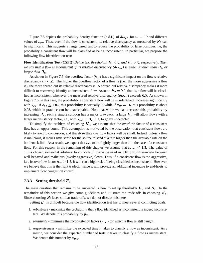
Figure 7.5 depicts the probability density function (p.d.f.) of� � � � � � for

� � � and differentvalues of

���� . Thus, even if the flow is consistent, its relative discrepancy as measured by

� � canbe significant. This suggests a range based test to reduce the probability of false positives, i.e, theprobability a consistent flow will be classified as being inconsistent. In particular, we propose thefollowing flow identification test:

Flow Identification Test (CSFQ) Define two thresholds: � �

��, and � � � �

, respectively. Thenwe say that a flow is inconsistent if its relative discrepancy (

� � � � � � ) is either smaller than � � , orlarger than � � .

As shown in Figure 7.5, the overflow factor (���� ) has a significant impact on the flow’s relative

discrepancy (� � � � � � ). The higher the overflow factor of a flow is (i.e., the more aggressive a flow

is), the more spread out its relative discrepancy is. A spread out relative discrepancy makes it moredifficult to accurately identify an inconsistent flow. Assume � � � � ��� , that is, a flow will be classi-fied as inconsistent whenever the measured relative discrepancy (

� � � � � � ) exceeds� ��� . As shown in

Figure 7.5, in this case, the probability a consistent flow will be misidentified, increases significantlywith

���� . If

����� �� � � , this probability is virtually 0, while if

���� � � , this probability is about

0.03, which in practice can be unacceptable. Note that while we can decrease this probability byincreasing � � , such a simple solution has a major drawback: a large ��� will allow flows with alarger inconsistency factor, i.e., with

� �� � � � � , to go by undetected.

To simplify the problem of choosing � � , we assume that the overflow factor of a consistentflow has an upper bound. This assumption is motivated by the observation that consistent flows arelikely to react to congestion, and therefore their overflow factor will be small. Indeed, unless a flowis malicious, it makes little sense for the source to send at a rate higher than the available rate on thebottleneck link. As a result, we expect that

���� to be slightly larger than 1 in the case of a consistent

flow. For this reason, in the remaining of this chapter we assume that���� �

� ���� . The value of1.3 is chosen somewhat arbitrary to coincide to the value used in [101] to differentiate betweenwell-behaved and malicious (overly aggressive) flows. Thus, if a consistent flow is too aggressive,i.e., its overflow factor

����� ���� , it will run a high risk of being classified as inconsistent. However,

we believe that this is the right tradeoff, since it will provide an additional incentive to end-hosts toimplement flow congestion control.

7.3.3 Setting threshold � �

The main question that remains to be answered is how to set up thresholds � � and � � . In theremainder of this section we give some guidelines and illustrate the trade-offs in choosing � � .Since choosing � � faces similar trade-offs, we do not discuss this here.

Setting � � is difficult because the flow identification test has to meet several conflicting goals:

1. robustness - maximize the probability that a flow identified as inconsistent is indeed inconsis-tent. We denote this probability by �

� .

2. sensitivity - minimize the inconsistency factor (� �� ) for which a flow is still caught.

3. responsiveness - minimize the expected time it takes to classify a flow as inconsistent. As ametric, we consider the expected number of tests it takes to classify a flow as inconsistent.We denote this number by �

�� .

116

In the remainder of this section, we assume that router�

= misbehaves by forwarding a constantfraction of inconsistent traffic

�� to

� � . The reason we assume that �� is constant is because,

as we will show in Section 7.4.1, this represents the worst case scenario for our flow identificationtest. In particular, if a malicious router wants to maximize the excess bandwidth received by itsinconsistent traffic before being caught, then it has to send inconsistent traffic at a constant fractionof its total traffic. Further, we assume that all consistent flows have

���� � ���� , and all inconsistent

flows have����� , i.e., no packet of an inconsistent flow is ever dropped by

�

= . As a result therelative discrepancy of an inconsistent flow will be exactly

� �� . This means that our test will not

be able to catch an inconsistent flow with� �� � � � � . Again, this choice of

���� represents the

worse-case scenario. It can be shown that decreasing the���� of consistent flows and/or increasing

the���� of inconsistent flows will only improve the test robustness, sensitivity, and responsiveness.

Next, we derive the two parameters that characterize the robustness and responsiveness: �

� ,

and � �� . By using Bayes’s formula and the notations in Table 7.1 we have

�

� � Pr � �

���� �

�� � (7.4)

� Pr � � �� � Pr � �

�� � �

�� �

Pr � � �� � Pr � �

�� � �

�� � � Pr � � � � Pr � �

�� � � � �

� ����

�� ;

��

����

�� ;

�� � ����

�� ��� � ;

�� �

In addition, the expected number of flows that are tested before a flow will be classified asinconsistent, �

�� , is

� �� �

�=� ����� � � �

;>= �

�� �

�

���

(7.5)

where �

�� is the probability that a selected flow will be classified as inconsistent. With the notations

from Table 7.1, and using simple probability manipulations, we have

�

�� � � � Pr � �

�� � (7.6)

� � � � Pr � � ���� �

�� � � Pr � �

���� � � � �

� � � � Pr � � �� � Pr � �

�� � �

�� ��� Pr � � � � Pr � �

�� � � � � �

� � ��� ����

�� ;

�� � ���

�� ��� � ;

�� �

Finally, by combining Eqs. (7.5) and (7.6), we obtain

� �� �

� ��� ����

�� ;

�� � ����

�� ��� � ;

�� � � (7.7)

As illustrated by Eqs. (7.4) and (7.7), the fraction of the inconsistent traffic, �� , has a critical

impact on both �

� and �

�� . The smaller

�� is, the smaller �

� is, and the larger �

�� is. The

reason � �� increases when

�� decreases is because in any valid flow identification test we have

�

�� ;

�� � � � ;

�� , i.e., the probability an inconsistent flow will be identified is always larger than

the probability a consistent flow will be misidentified. In the remainder of this chapter, we choose a

117

0

0.2

0.4

0.6

0.8

1

0 0.05 0.1 0.15 0.2 0.25 0.3 0.35 0.4

p_id

H_u

k_inc = 1.05k_inc = 1.1

k_inc = 1.15k_inc = 1.2

k_inc = 1.25k_inc = 1.3

(a)

1

10

100

1000

0 0.05 0.1 0.15 0.2 0.25 0.3 0.35 0.4 0.45

n_in

c

H_u

k_inc = 1.05k_inc = 1.1

k_inc = 1.15k_inc = 1.2

k_inc = 1.25k_inc = 1.3

(b)

Figure 7.6: (a) The probability to identify an inconsistent flow, � � ( , and (b) the expected number of tests ittakes to classify a flow as inconsistent, �7� ��� , as functions of � & . (The values of ��� �)� for �)� ��� � � � � and� & � � � . are not plotted as they are larger than � � .) All inconsistent flows have � $ � � , � ��� � ��� , and� � � .

somewhat arbitrary �� � � � . If

���� � , we simply ignore the impact of the inconsistent traffic

on the consistent traffic. This decision is motivated by the fact that the inconsistent traffic can “steal”at most a fraction,

�� , of the link capacity. In the worst case, this leads to a 10% degradation in the

bandwidth received by a consistent flow, which we consider to be acceptable. However, it should benoted that there is nothing special about this value of

�� . The reason for which we use a specific

value for �� is to make the procedure of choosing � � more concrete.

Without loss of generality, we assume � � � , i.e., once a flow is selected, it remains active forat least � �

�. Note that if � �

� , this will simply result in scaling up �

�� by �� � � . Probabilities

�

�� ;

�� and � � ;

�� are computed based on the p.d.f. of the relative discrepancy. Figure 7.6(a) plots

then the probability to identify an inconsistent flow, �

� , while Figure 7.6(b) plots the expected num-

ber of tests to classify a flow as inconsistent, � �� . These plots illustrate the trade-offs in choosing

� � . On one hand, the results in Figure 7.6(a) suggest that we have to choose � �� � � � ; otherwise,

the probability to identify an inconsistent flow becomes smaller than 0.5. On the other hand, fromFigure 7.6(b), it follows that in order to make the test responsive we have to choose � � � � � � , as� �� starts to increase hyper-exponentially for ��� � � � � . To meet these restrictions, we choose

� �)� � � � . Note that this choice gives us the ability to catch any inconsistent flow as long as itsinconsistency factor (

� �� ) is greater than 1.2.

7.3.4 Increasing Flow Identification Test’s Robustness and Responsiveness

In the previous section we have assumed that� � � , where

�

represents the number of packetsthat can be sent during a monitoring interval at the fair rate by the upstream router

�

= . In thissection we study the impact of

�

on the flow identification test performances.Figures 7.7(a) and 7.7(b) plot the probability to identify an inconsistent flow, �

� , and the ex-

pected number of tests it takes to classify a flow as inconsistent, � �� , versus

� �� for various values

of�

. As shown in Figure 7.7(a), increasing�

can dramatically improve the test robustness. In

118

0.2

0.3

0.4

0.5

0.6

0.7

0.8

0.9

1

1.2 1.22 1.24 1.26 1.28 1.3 1.32 1.34

p_id

k_inc

m = 10m = 20m = 30m = 40m = 50

(a)

5

10

15

20

25

30

35

1.2 1.22 1.24 1.26 1.28 1.3 1.32

n_in

c

k_inc

m = 10m = 20m = 30m = 40m = 50

(b)

Figure 7.7: (a) The probability to identify an inconsistent flow, � � ( , and (b) The expected number of tests toclassify a flow as inconsistent, �7� ��� , versus inconsistency factor, � � ��� , for various values of � .

addition, as shown in Figure 7.7(b), a large�

makes the identification test more responsive forvalues of

� �� closer to � � . However, it is important to note that, while a large

�

can signifi-cantly reduce �

�� , this does not necessary translate into a reduction of the time it takes to classify a

flow as inconsistent, i.e., �� . In particular, if a router monitors

�flows simultaneously, we have

�� � � �

�� �� � �

. Thus, an increase of�

results directly into an increase of the time it takes totest a flow for consistency, � �

�, an increase which can offset the decrease of �

�� .

7.4 Identifying Misbehaving Nodes

Recall that our main goal is to detect misbehaving routers or/and hosts. In this section we presentand discuss such a test.

Like a flow identification test, ideally, a node identification test should be (1) robust, (2) re-sponsive, and (3) sensitive. Unfortunately, it is very hard, if not impossible, to achieve these goalssimultaneously. This is to be expected as the node test is based on the flow identification test, andtherefore we are confronted with the same difficult trade-offs. Worse yet, the fact that the probabilityof a node misbehaving can be very low makes the problem even more difficult.

Arguably, the simplest node identification test would be to decide that an upstream node mis-behaves whenever a flow is classified as inconsistent. The key problem is that in a well engineeredsystem, in which the probability of a misbehaving node is very small, this test is not enough. Asan example, assume that we use

� � � � , and that our goal is to detect inconsistent flows with� �� � �� � � . Then, according to the results in Figure 7.7, we have �

� �

� � � � . Thus, there is a� � � � probability of false positives. In addition, assume that the probability that the upstream node�

= misbehaves is also� � � � . This basically means that whenever

� � classifies a flow as beinginconsistent there is only a 0.5 chance that this is because

�

= misbehaves!To alleviate this problem we propose a slightly more complex node identification test: instead

of using only one observation to decide whether a node misbehaves or not, we use multiple obser-vations. In particular we have the following test

119

Node Identification (CSFQ): Test 1 An upstream node is assumed to misbehave if at least � �flows out of the last

� � tested flows were classified as inconsistent, where � � and� � are predefined

constants.

Let�

denote the probability of false positives, that is, the probability that every time we identifyan inconsistent flow during the last

� � tests we were wrong. Assuming that the results of the flowidentification tests are independently distributed, we have:

� � �� ���� � �

� � �������� � �

�

� �

;

� � (7.8)

In the context of the previous example, assume that� � � � , and � � � � . This yields

� �� � � � � � . Thus, in this case, the probability that we are wrong is much smaller than the probabilitythat the node is misbehaving. In consequence, if three out of the last five tested flows are classifiedas inconsistent we can decide with high probability that the upstream node is indeed misbehaving.

A potential problem with the previous test is that a large threshold � � , will allow a misbehavingnode to inflict substantial damages without being caught. In particular, if a node inserts in the packetheaders a rate that is

� �� times larger than the actual flow rate, where

� �� �

�� � , the node will

get up to� �� � times more capacity for free without being caught. For example, in our case, when

� � � �� � , the upstream node can get up to 20% extra bandwidth.To filter out this attack we employ a second test. This test is based on the observation that in a

system in which all nodes are well-behaved the mean value of� � � � � � is expected to be zero. In this

case, any significant deviation of� � � � � � from zero is interpreted as being caused by a misbehaving

upstream node.

Node Identification (CSFQ): Test 2 An upstream node is assumed to misbehave if the mean valueof� � � � � � does not fall within � � � � � � .

7.4.1 General Properties

In this section we present two simple but important properties of our identification test. The firstproperty says that a misbehaving node can inflict maximum of damage when it sends inconsistenttraffic at a constant rate. In particular, the excess bandwidth received by the inconsistent traffic ata downstream router, before being caught, is maximized when the rate of the inconsistent traffic isconstant. This property is important because it allows us to limit our study to the cases in which athe fraction of the inconsistent traffic sent by a misbehaving node is constant. The second propertysays that a misbehaving node cannot hurt the downstream consistent traffic in a “big” way for a longtime. In other words, the higher the rate of the inconsistent traffic is, the faster the misbehavingnode is caught. The two properties are given below.

Property 1 Let� �� � � � � � denote the total volume of inconsistent traffic received by a router at

an input port during the interval � �� � � � . Then, the probability that no inconsistent flow is identifiedduring � � � � � , is minimized when the inconsistent traffic arrives at a fixed rate �

�� , where �

�� �

� �� � � � � � � � � � � � .

120

Proof. Let �

�� � � � be the rate of the inconsistent traffic at time � , and let � denote the input link

capacity where the traffic arrives. Then, the fraction of the inconsistent traffic at time � is �� � � � �

�

�� � � � � � , where the equality occurs when the link is fully utilized. Let � = , � � , � � � , �

�be the time

instants when a new flow is selected to be monitored during the interval � � � � � . By using Eq. (7.6),the probability that none of these flows will be identified as being inconsistent, denoted � , is

� �

��� = ��� �

�� � �� � (7.9)

�� ��� � �

�� = �

�� � ����

�� ;

�� � ����

�� � �� ��� � ;

���

�� �

�� ��� � �

�� =

�� � ��

� �

�� ;

�� ��� � �

�� = ��

�� � ��

� � � ;

��� �

�

Since a router randomly selects a flow to be monitored, we assume without loss of generality that� = , � � , � � � , �

�are independently distributed within � �� � � � . By assuming that �

�� � � � is a continuous

function over the interval � � � � � , we have

�

�� � Exp

� ��� = �

�� � ��

��� (7.10)

In addition, since �� � � � � �

�� � � � � � , for any � , the following inequality follows trivially

��� =

�� � ��

�� �

�� = �

�� � ��

��� � (7.11)

By combining Eqs. (7.9), (7.11) and Eq. (7.10), using the fact that �� , � � , �

�� ;

�� and � � ;

�� are

independently distributed variables, and the fact that �

�� ;

�� �)� � ;

�� , we obtain

Exp ��� � ���� Exp �-� � � �

��� Exp �-�

�� ;

�� � � Exp �-� � �

��� �

����

Exp �-� � ; �� �� �

(7.12)

� ��� Exp �-� � �� ���

Exp �-� �� ;

�� � � Exp �-� � �

����

�� ��

Exp �-� � ; �� � ��

where �� � �

�� � � . But the last term in the above inequality represents exactly the expected

probability a flow will not be classified as inconsistent after � tests, when the inconsistent trafficarrives at a fixed rate. This concludes the proof of the property.

Thus, if the fraction at which a misbehaving node sends inconsistent traffic fluctuates, the prob-ability to identify an inconsistent flow can only increase. This is exactly the reason we have consid-ered in this chapter only the case in which this fraction, i.e.,

�� , is constant.

Property 2 The higher the rate of the inconsistent traffic is, the higher the probability to identifyan inconsistent flow is.

Proof. The proof follows immediately from Eq. (7.4) and the fact that in a well designed flowidentification test, the probability an inconsistent flow will be identified, �

�� ;

�� , should be larger

than the probability a consistent flow will be misidentified, � � ;

�� .

121

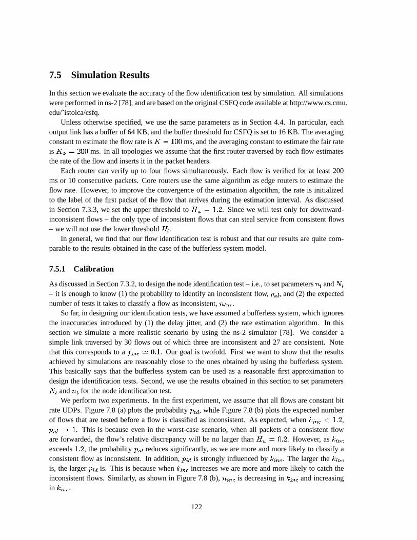
7.5 Simulation Results

In this section we evaluate the accuracy of the flow identification test by simulation. All simulationswere performed in ns-2 [78], and are based on the original CSFQ code available at http://www.cs.cmu.edu/˜istoica/csfq.

Unless otherwise specified, we use the same parameters as in Section 4.4. In particular, eachoutput link has a buffer of 64 KB, and the buffer threshold for CSFQ is set to 16 KB. The averagingconstant to estimate the flow rate is �*� � � ms, and the averaging constant to estimate the fair rateis � � � � � � ms. In all topologies we assume that the first router traversed by each flow estimatesthe rate of the flow and inserts it in the packet headers.

Each router can verify up to four flows simultaneously. Each flow is verified for at least 200ms or 10 consecutive packets. Core routers use the same algorithm as edge routers to estimate theflow rate. However, to improve the convergence of the estimation algorithm, the rate is initializedto the label of the first packet of the flow that arrives during the estimation interval. As discussedin Section 7.3.3, we set the upper threshold to ��� � �� � . Since we will test only for downward-inconsistent flows – the only type of inconsistent flows that can steal service from consistent flows– we will not use the lower threshold � � .

In general, we find that our flow identification test is robust and that our results are quite com-parable to the results obtained in the case of the bufferless system model.

7.5.1 Calibration

As discussed in Section 7.3.2, to design the node identification test – i.e., to set parameters � � and� �

– it is enough to know (1) the probability to identify an inconsistent flow, �

� , and (2) the expected

number of tests it takes to classify a flow as inconsistent, � �� .

So far, in designing our identification tests, we have assumed a bufferless system, which ignoresthe inaccuracies introduced by (1) the delay jitter, and (2) the rate estimation algorithm. In thissection we simulate a more realistic scenario by using the ns-2 simulator [78]. We consider asimple link traversed by 30 flows out of which three are inconsistent and 27 are consistent. Notethat this corresponds to a

�� � � � . Our goal is twofold. First we want to show that the results

achieved by simulations are reasonably close to the ones obtained by using the bufferless system.This basically says that the bufferless system can be used as a reasonable first approximation todesign the identification tests. Second, we use the results obtained in this section to set parameters

� � and � � for the node identification test.We perform two experiments. In the first experiment, we assume that all flows are constant bit

rate UDPs. Figure 7.8 (a) plots the probability �

� , while Figure 7.8 (b) plots the expected number

of flows that are tested before a flow is classified as inconsistent. As expected, when� ���

�� � ,�

��� . This is because even in the worst-case scenario, when all packets of a consistent flow

are forwarded, the flow’s relative discrepancy will be no larger than � � � � � � . However, as� ��

exceeds �� � , the probability �

� reduces significantly, as we are more and more likely to classify a

consistent flow as inconsistent. In addition, �

� is strongly influenced by

� �� . The larger the

� ��

is, the larger �

� is. This is because when

� �� increases we are more and more likely to catch the

inconsistent flows. Similarly, as shown in Figure 7.8 (b), � �� is decreasing in

� �� and increasing

in� �� .

122

0.1

0.2

0.3

0.4

0.5

0.6

0.7

0.8

0.9

1

1.05 1.1 1.15 1.2 1.25 1.3

p_id

k

k_inc = 1.2k_inc = 1.25k_inc = 1.3

(a)

10

100

1000

10000

1.05 1.1 1.15 1.2 1.25 1.3

n_in

c

k

k_inc = 1.2k_inc = 1.25

k_inc = 1.3

(b)

Figure 7.8: (a) The probability to identify an inconsistent flow, � � ( , and (b) the expected number of tests ittakes to classify a flow as inconsistent, �7� ��� . We consider 30 flows, out of which three are inconsistent.

�)� ��� � � ( ��� ���1.3 0.76 251.25 0.45 63.61.2 0.12 1151.15 0.025 6901.1 0 7001 0 720

Table 7.2: � � ( and � � ��� as a function of the parameter � � ��� of the inconsistent flows. We consider 27consistent TCP flows and 3 UDP inconsistent flows.

One thing worth noting here is that these results are consistent with the ones achieved in thesimplified bufferless system. For example, as shown in Figures 7.6(a) and 7.8(a), in both cases theprobability �

� for

� �� � ���� , �

�� � �� � � , and � � � � � � , is somewhere between 0.7 and 0.8.

This suggests that tuning the parameters in the bufferless system represents a reasonable first orderapproximation.

In the second experiment we assume that all the consistent flows are TCPs, while the inconsistentflows are again constant bit rate UDPs. The results are presented in Table 7.2. It is interesting tonote that although the TCP flows experience a dropping rate of only 5%, which would correspondto

� �� � �� � � , both �

� and �

�� are significantly worse than their corresponding values in the case

of the previous experiment when� ��/� �� � � . In fact, comparing the values which corresponds to�

�� � ���� in both Figure 7.8(a) and Table 7.2, the behavior of TCPs is much closer to a scenario in

which they are replaced by UDPs with� �� � ���� , rather than

� �� � �� � � . This is mainly because

the TCP burstiness negatively affects the rate estimation accuracy, and ultimately the accuracy ofour identification test.

In summary, for both TCP and UDP flows we take � � � � � � � and � ��/� � � . This means that

by using 25 observations, the probability to identify an inconsistent flow with� �� � ���� is greater

or equal to� � � � .

123

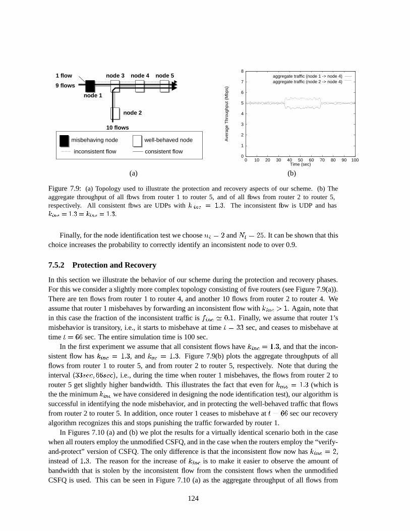
node 1

misbehaving node well-behaved node

node 2

node 5node 4node 3

10 flows

9 flows

1 flow

consistent flowinconsistent flow

(a)

0

1

2

3

4

5

6

7

8

0 10 20 30 40 50 60 70 80 90 100

Ave

rage

Thr

ough

put (

Mbp

s)

Time (sec)

aggregate traffic (node 1 -> node 4)aggregate traffic (node 2 -> node 4)

(b)

Figure 7.9: (a) Topology used to illustrate the protection and recovery aspects of our scheme. (b) Theaggregate throughput of all flows from router 1 to router 5, and of all flows from router 2 to router 5,respectively. All consistent flows are UDPs with � � �)� � � . . The inconsistent flow is UDP and has� � ��� � � . � � � ��� � � . .

Finally, for the node identification test we choose � � � � and� � � � � . It can be shown that this

choice increases the probability to correctly identify an inconsistent node to over 0.9.

7.5.2 Protection and Recovery

In this section we illustrate the behavior of our scheme during the protection and recovery phases.For this we consider a slightly more complex topology consisting of five routers (see Figure 7.9(a)).There are ten flows from router 1 to router 4, and another 10 flows from router 2 to router 4. Weassume that router 1 misbehaves by forwarding an inconsistent flow with

� �� � . Again, note that

in this case the fraction of the inconsistent traffic is �� � � � . Finally, we assume that router 1’s

misbehavior is transitory, i.e., it starts to misbehave at time � � � � sec, and ceases to misbehave attime � � � � sec. The entire simulation time is 100 sec.

In the first experiment we assume that all consistent flows have� �� � ���� , and that the incon-

sistent flow has� �� � ���� , and

���� � ���� . Figure 7.9(b) plots the aggregate throughputs of all

flows from router 1 to router 5, and from router 2 to router 5, respectively. Note that during theinterval ��� � ��'�� � � � ��'�� � , i.e., during the time when router 1 misbehaves, the flows from router 2 torouter 5 get slightly higher bandwidth. This illustrates the fact that even for

� �� � ���� (which is

the the minimum� �� we have considered in designing the node identification test), our algorithm is

successful in identifying the node misbehavior, and in protecting the well-behaved traffic that flowsfrom router 2 to router 5. In addition, once router 1 ceases to misbehave at � ��� � sec our recoveryalgorithm recognizes this and stops punishing the traffic forwarded by router 1.

In Figures 7.10 (a) and (b) we plot the results for a virtually identical scenario both in the casewhen all routers employ the unmodified CSFQ, and in the case when the routers employ the “verify-and-protect” version of CSFQ. The only difference is that the inconsistent flow now has

� ��/� � ,

instead of ���� . The reason for the increase of� �� is to make it easier to observe the amount of

bandwidth that is stolen by the inconsistent flow from the consistent flows when the unmodifiedCSFQ is used. This can be seen in Figure 7.10 (a) as the aggregate throughput of all flows from

124

0

1

2

3

4

5

6

7

8

0 10 20 30 40 50 60 70 80 90 100

Ave

rage

Thr

ough

put (

Mbp

s)

Time (sec)

aggregate traffic (node 1 -> node 4)aggregate traffic (node 2 -> node 4)

(a)

0

1

2

3

4

5

6

7

8

0 10 20 30 40 50 60 70 80 90 100

Ave

rage

Thr

ough

put (

Mbp

s)

Time (sec)

aggregate traffic (node 1 -> node 4)aggregate traffic (node 2 -> node 4)

(b)

Figure 7.10: Aggregate throughputs of all flows from router 1 to router 5, and from router 2 to router 5,when all routers implement (a) the unmodified CSFQ, and (b) the “verify-and-protect” version of CSFQ. Allconsistent flows are UDPs with � � ��� � � . . The inconsistent flow is UDP with � � ��� �/� , and �)� �)� � .

router 2 to router 5 is slightly less than 5 Mbps. In contrast, when the “verify-and-protect” versionis used, these flows get considerably more than 5Mbps. This is because once router 3 concludesthat router 1 misbehaves, it punishes all its flows by simply multiplying their labels by

� �� � � . As

a result, the traffic traversing router 1 gets only 33%, instead of 50%, of the link capacities at thesubsequent routers.

Finally, Figures 7.11 (a) and 7.11(b) plot the results for the case in which consistent flows arereplaced by TCPs. As expected, the results are similar: the “verify-and-protect” version of CSFQ isable to successfully protect and recover after router 1 stops misbehaving.

7.6 Summary

While the solutions based on SCORE/DPS have many advantages over traditional stateful solutions(see Chapter 4, 5, 6), they still suffer from robustness and scalability limitations when compared tothe stateless solutions. In particular, the scalability is hampered because the network core cannottranscend trust boundaries (such as the ISP-ISP boundaries), and therefore high-speed routers onthese boundaries must be stateful edge routers. The lack of robustness is because the malfunctioningof a single edge or core router could severely impact the performance of the entire network, byinserting inconsistent state in the packet headers.

In this chapter, we have proposed an approach to overcome these limitations. To achieve scal-ability we push the complexity all the way to the end-hosts. To address the trust and robustnessissues, all routers statistically verify whether the incoming packets carry consistent state. We callthis approach “verify-and-protect”. This approach enables routers to discover and isolate misbehav-ing end-hosts and routers. The key technique needed to implement this approach is flow verificationthat allows the identification of packets carrying inconsistent state. To illustrate this approach, wehave described the identification algorithms in the case of Core-Stateless Fair Queueing (CSFQ),and we have presented simulation results in ns-2 [78] to demonstrate its effectiveness.

125

0

1

2

3

4

5

6

7

8

0 10 20 30 40 50 60 70 80 90 100

Ave

rage

Thr

ough

put (

Mbp

s)

Time (sec)

aggregate traffic (node 1 -> node 4)aggregate traffic (node 2 -> node 4)

(a)

0

1

2

3

4

5

6

7

8

0 10 20 30 40 50 60 70 80 90 100

Ave

rage

Thr

ough

put (

Mbp

s)

Time (sec)

aggregate traffic (node 1 -> node 4)aggregate traffic (node 2 -> node 4)

(b)

Figure 7.11: Aggregate throughputs of all flows from router 1 to router 5, and from router 2 to router 5,when all routers implement (a) the unmodified CSFQ, and (b) the “verify-and-protect” version of CSFQ. Allconsistent flows are TCPs. The inconsistent flow is UDP with � � ��� �/� , and �)� ��� � .

A final observation is that the “verify-and-protect” approach can also be useful in the contextof stateful solutions. Based only on the traffic a router sees, these solutions are not usually able totell whether there is a misbehaving up-stream router or not. For example, with Fair Queueing thereis no way for a router to discover an up-stream router that spuriously drops packets, as it cannotdifferentiate between a flow whose packets were dropped by a misbehaving router, and a flow whojust sends fewer packets. Thus, the “verify-and-protect” approach can be also used to effectivelyincrease the robustness of the traditional stateful solutions.

126

Chapter 8

Prototype Implementation Description

In Chapters 4, 5 and 6 we have presented three applications of our SCORE/DPS solution to providescalable services in a network in which core routers maintain no per flow state. In this chapter,we describe a prototype implementation of our solution. In particular, we have fully implementedthe functionalities required to provide guaranteed and flow protection services. While section 5.5presents several experimental results, including overhead measurements of our prototype, this chap-ter focuses on the implementation details.

The main goal of the prototype implementation is to show that it is possible to efficiently de-ploy our algorithms in today’s IPv4 networks with minimum incompatibility. To prove this pointwe have implemented a complete system, including support for fine grained monitoring, and easyconfiguration. The current prototype is implemented in FreeBSD v2.2.6, and it is deployed in a test-bed consisting of 300 MHz and 400 MHz Pentium II PCs connected by point-to-point 100 MbpsEthernets. The test-bed allows the configuration of a path with up to two core routers.

Although we had complete control of our test-bed, and, due to resource constraints, the scaleof our experiments was rather small (e.g., the largest experiment involved just 100 flows), we havedevoted special attention to making our implementation as general as possible. For example, whilein the current implementation we re-use protocol space in the IP header to store the DPS state, wemake sure that the modified fields can be fully restored by the egress router. In this way, the changesoperated by the ingress and core routers on the packet header are completely transparent to theoutside world. Similarly, while the limited scale of our experiments would have allowed us to usesimple data structures to implement our algorithms, we try to make sure that our implementationis scalable. For example, instead of using a simple linked list to implement the CJVC scheduler,we use a calendar queue together with a two-level priority queue to efficiently handle a very largenumber of flows (see Section 8.1).

For debugging and management purposes, we have implemented full support for packet levelmonitoring. This allows us to visualize simultaneously and in real-time the throughputs and thedelays experienced by flows at different points in the network. A key challenge when implementingsuch a fine grained monitoring functionality is to minimize the interferences with the system oper-ations. We use two techniques to address this challenge. First, we off-load as much as possible ofthe processing of log data on an external machine. Second, we use raw IP to send the log data fromrouter’s kernel directly to the external machine. This way, we avoid context-switching between thekernel and the user level.

To easily configure our system, we have implemented a command line configuration tool. This

127

tool allows us (1) to configure routers as ingress, egress, or core, (2) set-up, modify, and tear-downa reservation, and (3) set-up the monitoring parameters. To minimize the interferences betweenthe configuration operations and data processing, we implement our tool on top of the InternetControl Management Protocol (ICMP). Again, by using ICMP, we avoid context-switching whenconfiguring a router.

The rest of the chapter is organized as follows. The next section presents details of the mainoperations implemented by the data and control paths. Section 8.2 describes encoding techniquesused to efficiently store the DPS state in the packet headers. Section 8.3 presents our packet levelmonitoring tool, while Section 8.4 describes the configuration tool. Finally, Section 8.5 concludesthis chapter.

8.1 Prototype Implementation

For all practical purposes, a FreeBSD PC implements an output queueing router. Output interfacesusually employ a FIFO scheduling discipline, and drop-tail buffer management. Upon a packetarrival, the router performs a routing table lookup, based on the packet destination address, to deter-mine to which output interface the packet should be forwarded. If the output link is idle, the packetis passed directly to the device driver of that interface. Otherwise, the packet is inserted at the tailof the packet queue associated to the interface, by using the IF ENQUEUE macro.

When the output link becomes idle, or when the network card can accept more packets, a hard-ware interrupt is generated. This interrupt is processed by the device driver associated with the net-work card. As a result, the packet at the head of the queue is dequeued (by using the IF DEQUEUE

macro) and sent to the network card.Our implementation is modular in the sense that it requires few changes to the FreeBSD legacy

code. The major change is to replace the queue manipulation operations implemented by IF ENQUEUE

and IF DEQUEUE. In particular, we replace

IF_ENQUEUE(&ifp->if_snd, mb_head);

with

if (ifp->node_type)dpsEnqueue(ifp, (void **)&mb_head);

elseIF_ENQUEUE(&ifp->if_snd, mb_head);

In other words, we first check whether the router is configured as a DPS router or not, and if yes,we call dpsEnqueue to enqueue the packet1 in a special data structure maintained by DPS. If not,we simply use the default IF DEQUEUE macro. Similarly, we replace

IF_DEQUEUE(&ifp->if_snd, mb_head);

1Internally, FreeBSD stores packets in a special data structure called mbuf. An ordinary mbuf can store up to 108bytes of data. If a packet is larger than 108 bytes, a chain of mbufs is used to store the packet. mb head represents thepointer to the first mbuf in the chain.

128

with

if (ifp->node_type)dpsDequeue(ifp, &mb_head);

elseIF_DEQUEUE(&ifp->if_snd, mb_head);

In the current implementation, we support two device drivers: the Intel EtherExpress Pro/100BPCI Fast Ethernet driver, and the DEC 21040 PCI Ethernet Controller. As a result, the above changesare limited to three files: if ethersubr.c, which implements the Ethernet device-dependent function-ality, and if de.c and if fxp.c that implement the device-dependent functionalities for the two driverswe support.

In the remainder of this section, we present implementation details for the operations performedby our solution on both the data and control paths. All the processing is encapsulated by the dpsEn-queue and dpsDequeue functions. The implementation is about 5,000 lines.

8.1.1 Updating State in IP Header

Before forwarding a packet, a core router may update the information carried in its header. Forexample, in the case of Core-Stateless Fair Queue (CSFQ), if the estimated rate carried by a packet islarger than the link’s fair rate, the router has to update the state carried by the packet (see Figure 4.3).Similarly, with Core-Jitter Virtual Clock (CJVC), a router has to insert the “ahead of schedule”variable, , before forwarding the packet (see Figure 5.3).

Updating the state involves two operations: encoding the state, and updating the IP checksum.State encoding is discussed in details in Section 8.2. The checksum is computed as the 1’s comple-ment over the IP header, and therefore it can be easily updated in an incremental fashion.

8.1.2 Data Path

In this section we present the implementation details of the main operations performed by ingressand core routers on the data path: packet classification, buffer management, and packet scheduling.Since the goal of our solution is to eliminate the per flow state from core routers, we will concentrateon operation complexity at these routers. (The exception is packet classification which is performedby ingress routers only.)

8.1.2.1 Packet Classification

Recall that in SCORE/DPS only ingress routers need to perform packet classification. Core routersdo not, as they process packets based only on the information carried in the packet headers.

Our current prototype offers only limited classification capabilities.2 In particular, a class isdefined by fully specifying the source and destination IP addresses, the source and destination portnumbers, and the protocol type. This allows us to implement packet classification by using a simplehash table [26], in which the keys are computed by xor-ing all fields in the IP header that are usedfor classification.

2This can be easily fixed, by replacing the current classifier with the more complete packet classifier developed in thecontext of the Darwin project at Carnegie Mellon University [19].

129

6 …… 5

5, 8

5, 9 5, 10

5, 15

system time5

10 12

1, 12

4, 20 3, 15

2, 5

3, 10

2, 10

6 …… 5

system time 5

8 12

1, 12

4, 20 3, 15

2, 5

3, 10

10

2, 10

5, 8

5, 9 5, 10

5, 15

rate-regulator scheduler

(a)

(b)

Figure 8.1: Data structures used to implement CJVC. The rate-regulator is implemented by a calendar queue,while the scheduler is implemented by a two-level priority queue. Each node at the second level (and eachnode in the calendar queue) represents a packet. The first number represents the packet’s eligible time; thesecond its deadline. (a) and (b) show the data structures before and after the system time advances from 5 to6. Note that all packets that become eligible are moved in one operation to the scheduler data structure.

8.1.2.2 Buffer Management

With both CJVC and CSFQ, routers do not need to maintain any per flow state to perform buffermanagement. In particular, with CSFQ, packets are dropped probabilistically based on the flowestimated rate carried by the packet header, and the link fair rate (see Figure 4.3 and 4.4). In the caseof CJVC, we simply use a single drop-tail queue for all the guaranteed traffic. This is made possibleby the fact that, as we have discussed in Section 5.3.3, a relatively small queue can guarantee witha very high probability that no packets are ever dropped. For example, for all practical purposes, a8,000 packet queue can handle up to one million flows!

8.1.2.3 Packet Scheduling

With CSFQ, the scheduling is trivial as the packets are transmitted on a Fist-In-First-Out basis. Incontrast, CJVC, is significantly more complex to implement. With CJVC, each packet is assignedan eligible time and a deadline upon its arrival. A packet becomes eligible when the system timeexceeds the packet’s eligible time. The eligible packets are then transmitted in the increasing orderof their deadlines. Similar to other rate-controlled algorithms [112, 126], we implement CJVC using

130

a combination of a calendar queue and a priority queue [10].The calendar queue performs rate-regulation, i.e., it stores packets until they become eligible.

The calendar queue is organized as a circular queue in which every entry corresponds to a timeinterval [15]. Each entry stores the list of all packets that have the eligible times in the rangeassigned to that entry. When the system time advances past an entry, all packets in that entrybecome eligible, and they are moved in a priority queue. The priority queue maintains all eligiblepackets in decreasing order of their deadlines. Scheduling a new packet reduces then to the selectionof the packet at the head of the priority queue, i.e., the packet with the smallest deadline.

The algorithmic complexity of the calendar queue depends on how packets are stored within anentry. If they are maintained in a linked list, then the insertion and deletion of a packet are constanttime operations. In contrast, insertion and deletion of a packet in the priority queue takes ��� � ��� ��� ,where � is the number of packets stored in the priority queue [26]. Thus the total cost per packetmanipulation is � � ����� ��� .

While the above implementation is quite straightforward, it has a significant drawback. Asdescribed above, when the system time advances, all packets in an entry become simultaneouslyeligible, and they have to be transferred in the scheduler priority queue. The problem is that, atleast theoretically, the number of packets that become eligible can be unbounded. Moreover, sincethe packets are maintained in a simply linked list, we need to move them one-by-one! Thus, ifwe have to move

�

packets, this will take ��� � ����� ��� . Clearly, in a large system this solution isunacceptable, as it may result in packets missing their deadlines due to the large processing timerequired to move all packets from a calendar queue entry.

To address this problem, we store all packets that belong to the same calendar queue entry ina priority queue ordered by the packets’ deadlines. This way, when these packets become eligible,we can move all of them in the scheduler data structure in one step. To achieve this, we change thescheduler data structure to a two-level priority queue. Figure 8.1 illustrates the new data structuresin the context of a movement operation. Thus, with the new data structures, we reduce the time ittakes to move all packets from a calendar queue entry into the scheduler data structure to � � ����� ��� .

A final point worth noting is that the number of packets, � , that are stored at any time in thesedata structures is, with a very high probability, much smaller than the total number of active flows.As discussed in Section 5.3.3, this is an artifact of the fact that flows are aggressively regulated ateach node in the SCORE domain.

8.1.3 Control Path

Providing per flow isolation does not require any operations on the control path. In contrast, pro-viding guaranteed services requires a signaling mechanism to perform per flow admission control.However, as described in Section 5.4, the implementation of admission control at the core routers isquite straightforward. For each output link, a router maintains a value � that is updated every timea new packet arrives. Based on this value, the router periodically updates the upper bound of theaggregate reservation

���� ��� (see algorithm in Figure 5.6). Finally, to decide whether to accept a

new reservation or not, a core router just needs to perform a few arithmetic operations (again, seeFigure 5.6).

131

8.2 Carrying State in Data Packets

In order to eliminate the need for maintaining per flow state at each router, our DPS based algorithmsrequire packets to carry state in their headers. Since there is limited space in protocol headers andmost header bits have been allocated, the main challenge to implementing these algorithms is to(a) find space in the packet header for storing DPS variables and at the same time remain fullycompatible with current standards and protocols; and (b) efficiently encode state variables so thatthey fit in the available space without introducing too much inaccuracy. In the remainder of thesection, we present our approach to address the above two problems in IPv4 networks.

There are at least three alternatives to encode the DPS state in the packet headers:

1. Use a new IP option. (Note that DPS has been already assigned IP option number 23 by theInternet Assignment Number Authority (IANA) [56].)

From the protocol point of view, this is arguably the least intrusive approach, as it requiresno changes to IPv4 or IPv6 protocol stacks. The downside is that using the IP option can adda significant overhead. This can happen in two ways. First, most of today’s IPv4 routers arevery inefficient in processing the IP options [109]. Second, the IP option increases the packetlength, which can cause packet fragmentation.

2. Introduce a new header between the link layer and the network layer, similar to the way labelsare transported in Multi-Protocol Label Switching (MPLS) [17].

Like the previous approach, this approach does not require any changes in the IPv4/IPv6protocol stack. However, since each router has to know about the existence of the extra headerin order to correctly process the IP packets, this approach requires changes in all routers, nomatter whether this is needed to correctly implement the DPS algorithms or not. In contrast,with the IP option approach, if a router does not understand a new IP option, it will simplyignore it. In practice, this can be an important distinction, as many of today’s core routers aretypically uncongested. Thus, if we were to implement a service like flow protection, with theIP option approach we don’t need to touch these routers, while with this approach we need tochange all of them.

An additional problem is that this approach requires us to devise different solutions for dif-ferent link layer technologies. Finally, note that it also suffers from a fragmentation problem,since the addition of the extra header will increase the size of the packet.

Another option to implement this approach would be to leverage MPLS, whenever possible.In particular, in a network that implements MPLS, a solution would be to use an extra MPLSlabel to encode the DPS state.

3. Insert the DPS state in the IP header. The main advantage of this approach is that it avoids thepenalty imposed by most IPv4 routers in processing the IP options, or the need of devisingdifferent solutions for different technologies as it would have been required by introducinga new header between the link and network layers. The main problem however is findingenough space to insert the extra information.

132

While the first two approaches are quite general and can potentially provide large space forencoding state variables, due to performance and easy of implementation reasons, we choose thethird approach in our current prototype.3

8.2.1 Carrying State in IP Header

The main challenge to carrying state in the IP header is to find enough space to insert this informa-tion in the header while remaining compatible with current standards and protocols. In particular,we want the network domain to be transparent to end-to-end protocols, i.e., the egress node shouldrestore the fields changed by ingress and core nodes to their original values. To achieve this goal, wefirst use four bits from the type of service (TOS) byte (now renamed the Differentiated Service (DS)field) which are specifically allocated for local and experimental use [75]. In addition, we observethat there is an ip off field of 13 bits in the IPv4 header to support packet fragmentation/reassemblywhich is rarely used. For example, by analyzing the traces of over 1.7 million packets on an OC-3link [77], we found that less than 0.22% of all packets were fragments.

Therefore, in most cases it is possible to use ip off field to encode the DPS values. This ideacan be implemented as follows. When a packet arrives at an ingress node, the node checks whethera packet is a fragment or needs to be fragmented. If neither of these are true, the ip off field in thepacket header will be used to encode DPS values. When the packet reaches the egress node, theip off is cleared. Otherwise, if the packet is a fragment, it is forwarded as a best-effort packet. Inthis way, the use of ip off is transparent outside the domain. We believe that forwarding a fragmentas a best-effort packet is acceptable in practice, as end-points can easily avoid fragmentation byusing a Minimum Transfer Unit (MTU) discovery mechanism. Also note that in the above solutionwe implicitly assume that packets can be fragmented only by egress nodes.

In summary, we have up to 17 bits available in the current IPv4 header to encode four statevariables (see Figure 8.4). The next section discusses some general techniques to efficiently encodethe DPS state.

8.2.2 Efficient State Encoding

One simple solution to efficiently encode the state is to restrict each state variable to only a smallnumber of possible values. For example if a state variable is limited to eight values, only three bitsare needed to represent it. While this can be a reasonable solution in practice, in our implementationwe use a floating point like representation to represent a wider range of values. To further optimizethe use of the available space we employ two additional techniques. First, we use the floating pointformat only to represent the largest value, and then represent the other value(s) as a fraction of thelargest value. In this way we are able to represent a much larger range of possible values. Second, inthe case in which there are states which are not required to be simultaneously encoded in the samepacket, we use the same field to encode them. Next, we present the floating point like format usedto encode large values.

Assume that � is the largest value carried by the packet, where � is a positive integer. Torepresent � we use an

�

bit mantissa and an � bit exponent. Since �� �

, it is possible to gain an

3This choice can be also seen as an useful exercise that forces us to aggressively encode the state in the scarce spaceavailable in the IP header.

133

void intToFP(int val, int *mantissa, int *exponent) {int nbits = get_num_bits(val);if (nbits <= m) {

*mantissa = val;*exponent = (1 << n) - 1;

} else {*exponent = nbits - m - 1;*mantissa = (val >> *exponent) - (1 << m);

}}

int FPToInt(int mantissa, int exponent) {int tmp;if (exponent == ((1 << n) - 1))return mantissa;

tmp = mantissa | (1 << m);return (tmp << exponent)

}

Figure 8.2: The C code for converting between integer and floating point formats. � represents the numberof bits used by the mantissa; � represents the number of bits in the exponent. Only positive values arerepresented. The exponent is computed such that the first bit of the mantissa is always 1, when the number is� � . By omitting this bit, we gain an extra bit in precision. If the number is � � we set by convention theexponent to � � to indicate this.

extra bit for mantissa. For this we consider two cases: (a) if �� � � we represent � as the closest

value of the form � � � , where � � � � � � � � = . Then, since the� � -th most significant bit in

the � ’s representation is always 1, we can ignore it. As an example, assume� � � , � � � , and

� � ��� � � � . Then � is represented as ��� ��� � , where � � ��� � � and � � . By

ignoring the first bit in the representation of � the mantissa will store� � , while the exponent will

be . (b) On the other hand, if �

�� � , the mantissa will contain � , while the exponent will be

�� � . For example, for

� ��� , � � � , and � ��� � � � , the mantissa is � � , while the exponentis ��� . Converting from one format to another can be efficiently implemented. Figure 8.2 showsthe conversion code in C. For simplicity, we assume that integers are truncated rather than roundedwhen represented in floating point.

By using�

bits for mantissa and � for exponent, we can represent any integer in the range� � � � � � � � = � ���� � � � ;>= ��� with a relative error bounded by � � ���� � � = � ���� � � = � . For example,

with 7 bits, by allocating � for mantissa and � for exponent, we can represent any integer in therange � �� � �

���= � � with a relative error bounded by � � � � � � � � � � � � ��� . Note that these bounds are

not necessary tight. Indeed, in this example, the worst cases occur when encoding the numbers� � , and � � � , which both have a mantissa of 8. In particular, � � � � � � � ��� is encoded as� � � � � , � � � , and has a relative error of ���

�� � � � � �� ��� � ,� � � � � � � � � � � ��� � � , while

� � � � � � � � � � is encoded as ��� � � , � � � , and has a relative error of � ��� � � .If another value

� � � is carried by the packet we store it as the fraction � � ��� . Assuming thatwe use

�

= bits to represent , the absolute error is bounded by � � �� � � � � � � � �� � � �� � � � � � � � �� � � .

134

16 13 012

0 07 5 2 13 0 15 14 13 12 0

0ToS byte (DS field) fragment offset (ip_off) field

used by IP forwardingor by Diffservunused

used by DPS

Figure 8.3: For carrying DPS state we use the four bits from the TOS byte (or DS field) reserved for localuse and experimental purposes, and up to 13 bits from the IP fragment offset.

The � in the denominators is a result of mapping � � � values to [0, 1], with � � � � representing1. Finally, it is easy to show that by representing � in floating point format with

�

bits for mantissaand � bits for exponent, and by using

�

= bits to encode�, the relative error of � � �

, denoted� ' � � ��� � � � � � , is bounded by

� � � � = �

� � � � = � �

�� '�� � ��� � � � � �

�

� � � = � � � � � = � �

�(8.1)

where we ignore the second order term �� � � � � =�� � � � � = � � � � .In the next sections, we describe in detail the state encoding in the case of both guaranteed and

flow protection services.

8.2.3 State Encoding for Guaranteed Service

With the Guaranteed service, we use three types of packets to carry the DPS state: (1) data packets,(2) dummy packets, and (3) reservation request packets. Below, we describe the state encoding ineach of these cases:

8.2.3.1 Data packet

As described in Chapter 5, there are four pieces of state that need to be encoded in a data packet:(1) the reserved rate � or equivalently ����� , where � is the packet length, (2) the slack delay � , ascomputed by Eq. (5.10), (3) the amount of time by which the packet was transmitted ahead ofschedule at the previous node, and (4)

�, as computed by Eq. (5.12). The first three pieces of state

are used to perform packet scheduling, while the last one is used to perform admission control. Allare positive values. Figure 8.4 shows the state encoding in this case. The first two bits represent thecode that identifies the state format. The rest of the 15 bits are allocated to four fields:

� a 1-bit flag, called T, that specifies how the next field, 8� , is interpreted

� a 3-bit field 8� . If � �, then 8� encodes the

�value. Otherwise, it encodes ��� ��� � ��8 � .

� a 4-bit field 8 � that encodes ��8 �� a 7-bit field 8 � that encodes � ��� � � .We make several observations. First, since 8 � encodes the largest value among all fields, we

represent it in floating point format. By using this format, with seven bits we can represent any

135

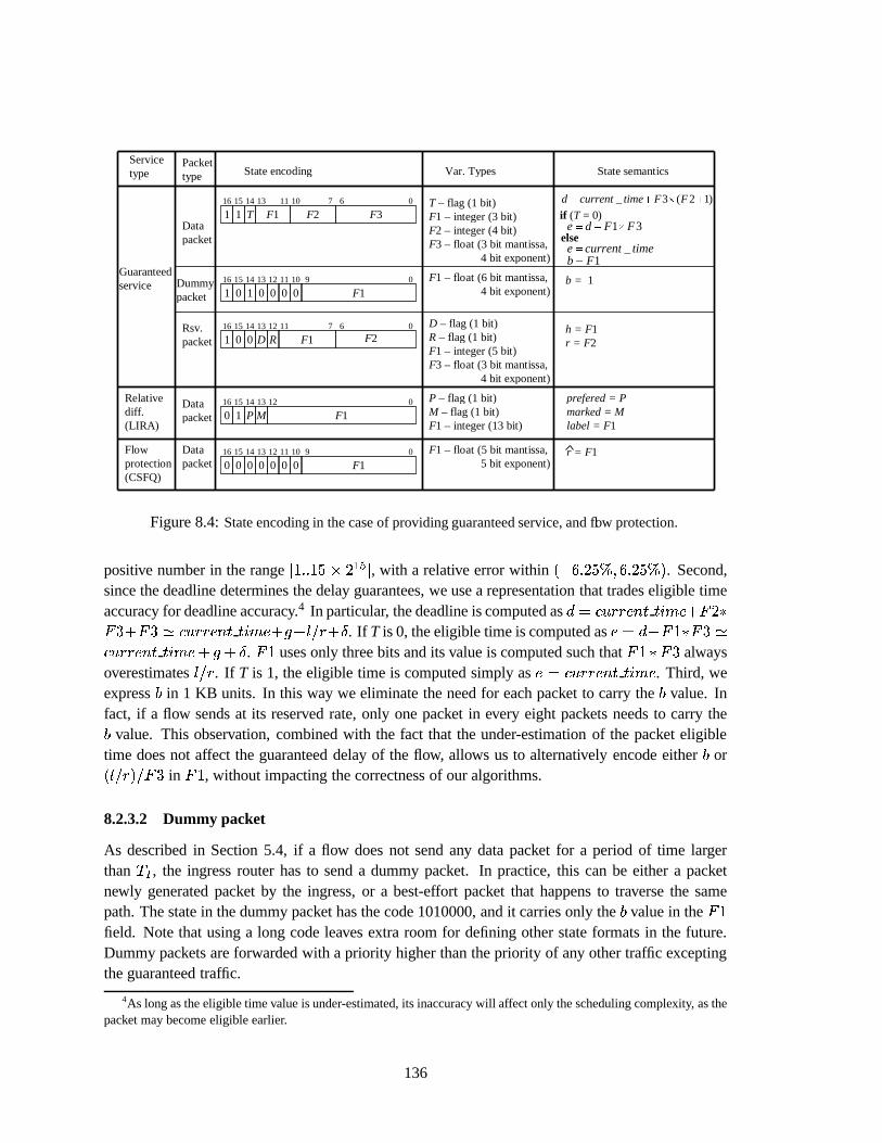
Guaranteedservice

T – flag (1 bit)F1 – integer (3 bit)F2 – integer (4 bit)F3 – float (3 bit mantissa,

4 bit exponent)

Data packet

1 1 T16 15 14 13 11 10 7 6 0

F1 F2 F3

1 0 016 15 14 13 0

1 0 116 15 14 13 10 9 0

F1 F2

D R F1 F212 11 7 6

0 0 0 F10 0 0 016 15 14 13 11 10 012 9

16 15 14 13 012 11

1 0 0 P A F1

Dummy packet

Rsv. packet

timecurrente _�

)12(3_ ���� FFtimecurrentd

1Fb �

if (T = 0)31 FFde ���

else

F1 – float (6 bit mantissa, 4 bit exponent)

D – flag (1 bit)R – flag (1 bit)F1 – integer (5 bit)F3 – float (3 bit mantissa,

4 bit exponent)

1 0 1 F10 0 0 016 15 14 13 11 10 012 9 b = 1

h = F1r = F2

Flowprotection(CSFQ)

F1 – float (5 bit mantissa, 5 bit exponent)

Data packet

State encoding Var. Types State semanticsPackettype

Servicetype

Relativediff. (LIRA)

Data packet 0 1 P F1M

16 15 14 13 012 P – flag (1 bit)M – flag (1 bit)F1 – integer (13 bit)

prefered = Pmarked = Mlabel = F1

r = F1

Figure 8.4: State encoding in the case of providing guaranteed service, and flow protection.

positive number in the range � �� � ��� = � � , with a relative error within � � � � � � � � � � � � � � . Second,

since the deadline determines the delay guarantees, we use a representation that trades eligible timeaccuracy for deadline accuracy.4 In particular, the deadline is computed as

�� � �����7' �>� � � � ' � 8 ���

8 � � 8 � � � �����7' �>� � � � ' � � � ��� � � . If T is 0, the eligible time is computed as '!�� � 8�� 8 � �

� �����7' �>� � � � ' � � � . 8� uses only three bits and its value is computed such that 8 �<8 � alwaysoverestimates ����� . If T is 1, the eligible time is computed simply as ' � � �����7' �>� � � � ' . Third, weexpress

�in 1 KB units. In this way we eliminate the need for each packet to carry the

�value. In

fact, if a flow sends at its reserved rate, only one packet in every eight packets needs to carry the�

value. This observation, combined with the fact that the under-estimation of the packet eligibletime does not affect the guaranteed delay of the flow, allows us to alternatively encode either

�or

��� ��� � ��8 � in 8� , without impacting the correctness of our algorithms.

8.2.3.2 Dummy packet

As described in Section 5.4, if a flow does not send any data packet for a period of time largerthan �� , the ingress router has to send a dummy packet. In practice, this can be either a packetnewly generated packet by the ingress, or a best-effort packet that happens to traverse the samepath. The state in the dummy packet has the code 1010000, and it carries only the

�value in the 8�

field. Note that using a long code leaves extra room for defining other state formats in the future.Dummy packets are forwarded with a priority higher than the priority of any other traffic exceptingthe guaranteed traffic.

4As long as the eligible time value is under-estimated, its inaccuracy will affect only the scheduling complexity, as thepacket may become eligible earlier.

136

8.2.3.3 Reservation request packet

This packet is generated by an ingress router upon receiving a reservation request. The ingressforwards this packet to the corresponding egress router in order to perform the requested reservation.Upon receiving this packet, a core router performs admission control, and updates the state carriedby the packet accordingly. When an egress router receives a reservation request packet, it sends itback to the ingress. Upon receiving this packet, the ingress router makes the final decision. Like thedummy packet, the reservation request packet can be either a newly generated packet, or a best-effortpacket that happens to traverse the same path.

The code of the state format carried by this packet is 101. The packet carries four fields in itsheader:

� a 1-bit field,�

, that denotes whether the packet traverses the forward or the backward path.If� � , the packet traverses the forwarding path; otherwise the packet is on its way back to

the ingress router that generated it.

� a 1-bit field,�

, which specifies the current state of the reservation request. If�� , then

all previous routers have accepted the reservation request; otherwise at least one router hasdenied it.

� a 5-bit field, 8� , that stores the number of hops, � , on the forwarding path. The field isincremented by each core router along the path. The number of hops is required to computethe slack variable of each packet at the ingress router (see Eq. (5.10)). Note that the currentimplementation allows a path with at most 32 hops. While this value does not cover thelengths of all end-to-end routes observed in today’s Internet, this value should be enough foran ISP domain, which is the typical SCORE domain.

� a 7-bit field that stores the requested rate. This rate is stored in floating point format, with a3-bit mantissa and a 4-bit exponent, and is expressed in 1 Kbps units.

8.2.4 State Encoding for LIRA

With LIRA, we use only one type of packet to carry the DPS state information. The first two bits arealways 01, and represent the code that identifies the state format. The rest of the 15 bits are dividedinto three fields as follows:

� a 1-bit flag,�

, called the preferred bit. This bit is set by the application or user and indicatesthe dropping preference of the packet. This bit is immutable, i.e., it cannot be modified byany router in the network.

� a 1-bit flag,�

, called the marking bit. This bit is set by the ingress routers of an ISP andindicates whether the packet is in- or out-of profile. When a preferred packet arrives at aningress node, the node marks it if the user has not exceeded its profile; otherwise the packet isleft unmarked. Whenever there is a congestion, a core router always drops unmarked packetsfirst. Irrespective of the congestion state, core routers never change the marked bit. The reasonwe use two bits (i.e., the marked and the preferred bits) instead of one is that in an Internet

137

environment with multiple ISPs, even if a packet may be out-of profile in some ISPs on theearlier portion of its path, it may still be in-profile in a subsequent ISP. Having the preferencebit that is unchanged by upstream ISPs on the path will allow downstream ISPs to make thecorrect decision.

� a 13-bit integer that represents the packet label. As discussed in Section 6.3.4, a label iscomputed as the XOR over the identifiers of all routers along the flow’s path. The length of arouter’s identifier is equal to the label’s length, i.e., 13 bit. The packet label is initialized by theingress router and updated by core routers as the packet is forwarded. Note that there is a non-zero probability that two labels may collide, i.e., that two alternate paths between the samerouters have the same label. If router identifiers are uniformly distributed, the probability ofcollision is �����= � �� � � � . While this probability cannot be neglected in practice, thereare two points worth noting. First, this problem can be alleviated by having the ISP choosethe router identifiers such that the probability of label collision is minimized. Second, notethat even if two alternate paths have the same label, the worst thing that may happen is analternate path will be ignored. Although this will eventually reduce the link utilization, it willnot jeopardize the correctness of our scheme.

8.2.5 State Encoding for CSFQ

As discussed in Chapter 4, with CSFQ, data packets carry only one piece of state: the estimated rateof the flow. In this case, we define a code of 010000, and a 10-bit field that encodes the estimatedrate, by using a floating point format with a 5-bit mantissa, and a 5-bit exponent. The estimated rateis initialized by the ingress router and then updated by core routers whenever the estimated rate isgreater than the fair rate on the output link (see Section 4.3).

By using a long code for the CSFQ state, we leave considerable room for defining future stateformats.

8.2.6 State Encoding Formats for Future Use

By inspecting the state encoding formats in Figure (8.4), it is easy to see that there is significantroom for future extensions. In particular, any state encoding format that starts with 001, 111, 1011,0001, 10101, 00001, 101001, 000001, 1010001 or 0000001 is available for future use. Thus, even byrestricting ourselves to reusing the space in the IP packet header, we can still design new DPS basedalgorithms and mechanisms that (at least at the level of the state encoding) are fully compatible tothe solutions proposed in this dissertation, and that can use up to 14 bits for specific state encoding.

8.3 System Monitoring

When implementing a network service, a key challenge is discovering whether the service is work-ing or not, and, more importantly, if it doesn’t work, finding out why. To help answer these questionswe need a monitoring tool that can accurately expose router behavior. Ideally, we want the abilityto monitor router’s behavior in real time, and at the smallest possible granularity, i.e., at the packet

138

flags fragment offset (13 bits)

total length (16 bits)

identification (16 bits)

header checksum (16 bits)TTL protocol

ToS4 IHL

source IP address (32 bits)

destination IP address (32 bits)

IP Packet Header

+arrival time (32 bits)

departure time (32 bits)

log type

Figure 8.5: The information logged for each packet that is monitored. In addition to most fields of the IPheader, the router records the arrival and departure times of the packet (i.e., the ones that are shaded). Thetype of event is also recorded, e.g., packet departure, or packet drop. The DPS state is carried in the ToS andthe fragment offset fields.

level. A key challenge when implementing such a fine grained monitoring functionality is to mini-mize the interferences to the monitored system.

A possible solution that fully addresses this challenge is to use a hub or a similar device be-fore/after each router’s interface to replicate the entire traffic and divert it to an external monitoringmachine where it can be processed. Unfortunately, there are two problems with this solution. First,it is very hard to accurately measure the arrival and the departure times of a packet. With a simplehub we can infer these times only when packets arrive at the monitoring machine. However, thepacket processing overhead at the monitoring machine can significantly impact the accuracy of thetime estimates. Even with a special device that can insert a timestamp in each packet when thepacket is replicated, the problem is not trivial. This is because the arrival and departure times ofa packet are inserted by two different devices, so we need a very accurate synchronization clockmechanism to minimize the errors. The second problem with this solution is that it requires anexpensive hardware infrastructure.

For these reasons, in our implementation we use an alternate approach. In particular, we in-strument the kernel to perform packet level monitoring. For each packet, we record the arrival andthe departure times with very high accuracy using the Pentium clock counter. In addition to thesetimes, with each packet we log most of the fields of the IP header, including the DPS state carriedby the packet, and a field, called log type, which specifies whether the packet was transmitted ordropped. To minimize the monitoring overhead, we use the ip output function call to send thisinformation directly from kernel to an external monitoring machine. Using ip output, instead ofioctl, for transferring log data, avoids unnecessary context switching between the kernel and theuser level. In addition, we off-load as much as possible of the log data processing to the monitoringmachine. The functions performed by a router are kept to minimum: a router has only to (1) logpacket arrival and departure times, and (2) send the log data to the monitoring machine. In turn, themonitoring machine performs the bulk of data processing, such as packet classification, and com-puting the rate and/or delay of a flow. To further reduce the monitoring overhead, we provide the

139

ability to sample the data traffic. In particular, we can configure the router to probabilistically logone out of every 2, 4, 16, or 64 packets. Finally, to eliminate possible interferences between thedata traffic and transferring the log data, we use a different network interface to send out the loginformation.

To visualize the monitoring information, we have developed a Graphical User Interface (GUI)written in Java. This tool offers the possibility of simultaneously plotting up to nine graphs in realtime. Each of the graphs can be independently configured. In particular, the monitoring tool allowsus to specify for each graph:

� the network interface to be monitored. This is specified by the IP address of the router towhich the interface is attached, and the IP address of the neighboring router that is connectedto the interface.

� the flows to be monitored at the selected network interface. In our case, a flow is identifiedby its source and destination IP addresses, its source and destination port numbers, and theprotocol type.

� the parameters to monitor. Currently the tool can plot the throughput and the delay of a flow.The throughput is averaged over a specified time period. The delay can be computed eitheras the minimum, maximum, or average packet delay over a specified period of time.

This flexibility allows us, for example, to simultaneously visualize the throughput and per-hopdelay of a flow at different hops, to visualize the throughput and the delay of a flow at the same hop,or to visualize the throughput of a flow at multiple time scales. As an example, Figure 3.5 shows ascreen snapshot of our monitoring tool. The top two plot show the throughputs of three flows at twoconsecutive hops. The bottom two plots show the delays of the same flows at the same hops.

8.4 System Configuration

As with any software system, we need the ability to configure our system. In particular, we wantthe ability to configure a router as an ingress, egress, or core, and to set-up the various parametersof the packet classifier and packet scheduler. In addition, in the case of the guaranteed service, wewant the ability to set-up, modify, and tear-down a flow reservation. One possible solution would beto use an ioctl function call. Unfortunately, this approach has a significant drawback. Since theexecution of ioctl is quite expensive – it requires context-switching between the kernel and theuser level – it can seriously interfere with the processing of the data traffic. At the limit, in the caseof the guaranteed traffic, this can result in packets missing their deadlines.

To avoid this problem, we use the Internet Control Management (ICMP) protocol. In particular,we have written a simple command line utility, called config dps, that can be used to config-ure routers and initialize their parameters via ICMP. To achieve this, we have extended the ICMPprotocol by adding two new messages: ICMP DPSREQ, and ICMP DPSREPLY.

140

8.4.1 Router Configuration

So far we have classified routers as edge and core routers, and the edge routers as ingress and egressrouters. While at the conceptual level this classification makes sense, in practice, this distinction isless clear. For example, an edge router can be either an ingress or egress depending on the directionof the traffic that traverses it. As a result, we need to configure at a finer granularity, i.e., at thenetwork interface level, instead of at the router level. We identify an interface by two IP addresses:the address of the router to which the interface is attached, and the address of the downstream routerconnected to the interface. We then use the following command to configure a network interface:

config_dps 2 node next_node type

The first parameter of the command, the number 2, specifies that an interface is being configured.The next two parameters specify the interface: node represents the IP address of the router whoseinterface is being configured, and next node specifies the IP address of the downstream routerthat is connected to the interface. Finally type specifies whether this interface is configured asbelonging to an ingress, egress, or core router.

8.4.2 Flow Reservation

In the case of the guaranteed service we need the ability to set-up, modify, and tear-down a flowreservation.

To set-up a new reservation we use the following command:

config_dps 3 ingress egress src_addr dst_addr src_port dst_portproto rsv_rate q_size

The first parameter, the number 3, specifies that this command requests a new reservation. The nexttwo parameters specify the ingress and egress routers which are the end-points of our reservation. Inaddition, we use these parameters to identify the interface of the ingress where the flow state is tobe instantiated. The next five parameters, src addr, dst addr, src port, dst port, and proto,respectively, identify the flow. Finally, the last two parameters specify the requested reservation (inKbps), and the buffer size to be allocated at the ingress for this flow (in packets).

To terminate a reservation, we use the following command:

config_dps 4 ingress egress src_addr dst_addr src_port dst_port

The first parameter, the number 4, represents the code of the deletion operation. The other parame-ters have the same meaning as in the previous command.

Finally, the command to update a reservation is virtually identical to setting-up a reservation. Infact, this operation is implemented by tearing down the existing reservation, and creating a new one.

8.4.3 Monitoring

As described in Section 8.3, our implementation provides support for fine grained monitoring. Tostart monitoring the traffic at a network interface, we use the following command:

141

config_dps 0 node next_node mon_node mon_port level

Again, the first parameter, the number 0 in this case, represents the operation code. The next two pa-rameters are used to identify the interface that we want to monitor, while mon node and mon port

represent the IP address (of the monitoring machine) and the port number where the log data is tobe transmitted. Finally, level specifies the sampling level. The routers probabilistically log onepacket out of � ��������� consecutive packets that arrive at the interface. To stop monitoring the traffic atan interface, we use the same command, but with the second parameter set to 1, instead of 0.

8.5 Summary

In this chapter, we have presented a prototype implementation of our solution to provide guaranteedand flow protection services in an IPv4 network. To the best of our knowledge this is the first imple-mentation that provides these services in a core stateless network architecture. We have describedthe operations performed by both edge and core routers on data and control paths, as well as anapproach that allows to efficiently encode the DPS state in the IP header by re-using some of theexisting fields. In addition, we have described two support tools that allow packet level monitoringin real-time, and easy system configuration.

We have implemented our solution in FreeBSD 2.2.6, and deployed it in a local test-bed thatconsists of four PC routers and up to 16 hosts. The results presented in Sections 3.2 and 5.5 showthat (1) the overhead introduced by our solution is acceptable, i.e., we can still saturate the 100Mbps, (2) the overhead increases very little with the number of flows (at least when the number offlows is no larger than 100), and (3) the scheduling mechanisms protect the guaranteed traffic sothat its performance is not affected by the best-effort traffic.

While implementing this prototype we have learned two valuable lessons. First, the monitoringtool proved very useful not only in debugging the system, but also in promptly finding unexpectedcauses of experiment failures. For example, in more than one instance, we were able to easilydiscover that we do not achieve the expected end-to-end performance, simply because the sourcedoes not correctly generate the traffic due to unexpected interference (such as someone inadvertentlyusing the same machine). Second, the fact that our solution does not require the maintenance ofdistributed per flow state has significantly simplified our implementation. In particular, we were ableto implement the entire functionality of the control path, which is notoriously difficult to implementand debug in the case of the stateful solutions such as RSVP [128], in just a couple of days.

However, our implementation suffers from some limitations that we hope to address in the fu-ture:

� The current test-bed is a local area network. We would like to perform similar tests in a largerinternetwork environment such as CAIRN [16].

� All the experiments were performed with synthetic loads. In the future, we would like toexperiment with real applications such as video conferencing or distributed simulations.

� The test-bed consists of only PC workstations. We would like to implement our algorithms incommercial routers.

142

� The current configuration tool does not offer any protection. Anyone who knows the ad-dress of our routers and the command format, can send ICMP messages to re-configure therouters. Providing an encryption mechanism to avoid malicious router re-configuration wouldbe useful.

143

144

Chapter 9

Conclusions and Future Work

In this chapter, we conclude the dissertation by (1) summarizing our contributions, (2) exposingsome fundamental limitations of current solutions, and (3) proposing several directions for futurework.

9.1 Contributions

One of the most important reasons behind the overwhelming success of the Internet is the statelessnature of its architecture. The fact that routers do not need to maintain any fine grained informationabout traffic makes the Internet both scalable and robust. However, these advantages come at aprice: today’s Internet provides only a minimalist service, the best effort datagram delivery. As theInternet evolves into a global communication infrastructure that is expected to support a plethoraof new applications such as IP telephony, interactive TV, and e-commerce, the existing best effortservice will no longer be sufficient. As a result, there is an urgent need to provide more powerfulservices such as guaranteed services and flow protection.

Over the past decade, there has been intense research toward achieving this goal. Two classes ofsolutions have been proposed: those maintaining the stateless property of the original Internet (e.g.,Differentiated Services), and those requiring a new stateful architecture (e.g., Integrated Services).While stateful solutions can provide more powerful and flexible services such as per flow guaranteedservices, and can achieve higher resource utilization, they are less scalable than stateless solutions.In particular, stateful solutions require each router to maintain and manage per flow state on thecontrol path, and to perform per flow classification, scheduling, and buffer management on the datapath. Since there can be a large number of active flows in the Internet, it is difficult, if not impossible,to implement such solutions in a scalable fashion. On the other hand, while stateless solutions aremuch more scalable, they offer weaker services.

The main contribution of this dissertation is to bridge the long-standing gap between statefuland stateless solutions. To achieve this goal, we have described a novel technique called DynamicPacket State (DPS). The key idea behind DPS is that, instead of having routers maintain per flowstate, packets carry the state. In this way, routers are still able to process packets on a per flowbasis, despite the fact that they do not maintain per flow state. Based on DPS, we have proposed anetwork architecture called Stateless Core (SCORE) in which core routers do not maintain any perflow state. Yet, by using DPS, we have demonstrated that, in a SCORE network, it is possible to

145

provide services which are as powerful and flexible as the services provided by a stateful network.In particular, we have developed complete solutions to address some of the most important problemsin today’s Internet:

� Flow protection (Chapter 4) We have proposed the first solution to provide protection on aper flow basis without requiring core routers to maintain any per flow state. To achieve thisgoal, we have used DPS to approximate the functionality of a reference network in whichevery router implements the Fair Queueing [31] discipline with a SCORE network in whichevery router implements a novel algorithm, called Core-Stateless Fair Queueing (CSFQ).

� Guaranteed services (Chapter 5) We have developed the first solution to provide per flowdelay and bandwidth guarantees. We have achieved this goal by using DPS to emulate thefunctionality of a stateful reference network in which each router implements Jitter VirtualClock [126] on the data path, and per flow admission control on the control path in a SCOREnetwork. To this end, we have proposed a novel scheduling algorithm, called Core-JitterVirtual Clock (CJVC), that provides the same end-to-end delay bounds as Jitter Virtual Clock,but, unlike Jitter Virtual Clock, does not require routers to maintain per flow state.

� Large spatial granularity service (Chapter 6) We have developed a stateless solution thatallows us to provide relative differentiation between traffic aggregates over large numbersof destinations. The most complex mechanism required to implement this service is route-pinning, for which traditional solutions require routers to either maintain per flow state, ormaintain state that is proportional to the square of the number of edge routers. By using DPS,we are able to significantly reduce this complexity. In particular, we propose a route-pinningmechanism that requires routers to maintain state which is proportional only to the number ofegress routers.

While the above solutions have many scalability and robustness advantages over existing state-ful solutions, they still suffer from robustness and scalability limitations in comparison. Systemrobustness is limited by the possibility that a single edge or core router may malfunction, insertingerroneous information in the packet headers, severely impacting performance of the entire network.In Chapter 7, we propose an approach, called “verify-and-protect”, that overcomes these limitations.We achieve scalability by pushing the complexity all the way to the end-hosts, thus eliminating thedistinction between edge and core routers. To address the trust and robustness issues, all routersstatistically verify that the incoming packets are correctly marked. This approach enables routers todiscover and isolate misbehaving end-hosts and routers.

To demonstrate the compatibility of our solutions with the existing protocols, we have presentedthe design and prototype implementation of the guaranteed service in IPv4 networks. In Chapter 8we propose both efficient state encoding algorithms, as well as an encoding format for the proposedsolutions.

The SCORE/DPS ideas have already made an impact in both research and industrial commu-nities. Since we have published the first papers [101, 104], several new and interesting resultshave been reported. They include both extensions and improvements to the original CSFQ algo-rithm [18, 25, 111], and generalizations of our solution to provide guaranteed services [129, 130].In addition, DPS-like techniques have been used to develop new types of applications such as IP

146

traceback [91]. Furthermore, we observe that it is possible to extend the current Differentiated Ser-vice framework [32] to accommodate algorithms using Dynamic Packet State. The key extensionneeded is to augment each Per Hop Behavior (PHB) with additional space in the packet header forstoring PHB specific Dynamic Packet State [107]. Such a paradigm will significantly increase theflexibility and capabilities of the services that can be built with a Diffserv-like architecture.

9.2 Limitations

While in this thesis we have shown that by using the DPS technique it is possible to implement someof the most representative Internet services (for which previous solutions required stateful networks)in a SCORE network, one important question still remains: What are the limitations of SCORE/DPSbased solutions? More precisely, is there any service implemented by stateful networks that cannotbe implemented by a SCORE network? In this section, we informally answer these questions.

In a stateful router, each flow is associated a set of state variables such as the length of a flow’squeue and the deadline of the packet at the head of the flow’s queue. In addition, a router maintainssome global state variables such as buffer occupancy or utilization on the output link. A routerprocesses a packet based on both the per flow state and the global state stored at the router. As anexample, upon a packet arrival, a router checks whether the buffer is full, and if not, discards thepacket at the tail of the longest queue to make room for the new packet.

In contrast, in SCORE, a core router processes packets based on the state carried in packetheaders, instead of per flow state (as these routers do not maintain any such state). Thus, in or-der to emulate the functionality of a stateful router, a stateless router has to reconstruct the perflow state from the state carried in the packet headers. The question of what are the limitations ofSCORE/DPS based solutions reduces then to the question of what types of per flow state cannot beexactly reconstructed by core routers. We are aware of two instances in which current techniquescannot reconstruct the per flow state accurately:

1. The state of a flow depends on the behavior of other competing flows. Intuitively, this isbecause it is very hard, if not impossible, to encode the effects of this dependence in the packetheaders. Indeed, this would require a router to know the future behavior of the competingflows at the next router before updating the state in the packet headers.

Consider the problem of exactly emulating the Fair Queueing (FQ) discipline. Recall thatFQ is a packet level realization of a bit-by-bit round robin: if there are � backlogged flows,FQ allocates �� � of the link capacity to each flow. In the packet system, a flow is said to bebacklogged if it has at least one packet in the queue.

The challenge of implementing FQ in a stateless router is that the number of backloggedflows, and therefore the service received by a flow, is a highly dynamic parameter, i.e., itcan change every time a new packet arrives or departs. Unfortunately, it is very hard if notimpossible for a router to accurately update the number of backlogged flows when such anevent occurs. To illustrate this point, consider a packet arrival event.

When a packet of an idle flow arrives, the flow becomes backlogged, and the number of back-logged flows increases by one. Because the router does not maintain per flow state, the only

147

way it can infer this information is from the state carried in the packet header (as this is theonly new information that enters the system). However, inserting the correct information inthe packet header would require up-stream routers to know how many packets are in the flow’squeue when the packet arrives at the current node. In turn, this would require knowledge ofhow much service the flow has received at the current node so far, as this determines howmany packets are still left in the queue. Unfortunately, even if we were using a feedbackprotocol to continuously inform the up-stream routers of the state of the current router, thepropagation delay poses fundamental limitations on the accuracy of this information. Forexample, during the time it takes the information to reach the up-stream routers, an arbitrarynumber of flows may become backlogged!

2. The state of a flow depends on parameters that are unique to each router. Intuitively, this isbecause it is very hard to reconstruct these parameters at each router given the limited spacein the packet headers.

Consider a router that implements the Weighted Fair Queueing (WFQ) scheduling discipline.Similar to FQ, WFQ is a realization of a weighted bit-by-bit round robin: a flow � with weight�

receives � �� � � � � � � � of the link capacity, where � is the set of backlogged flows.

Assume that the flow has a different weight at every router along its path. Then, each packethas to encode all these weights in its header. Unfortunately, in the worst case, encodingthese weights requires an amount of state proportional to the length of the path, which is notacceptable in practice.

Not surprisingly, these limitations are reflected in our solutions. The first limitation is the mainreason why Core Stateless Fair Queueing is only able to approximate, not emulate, the Fair Queue-ing discipline. Similarly, it is the main reason why our per flow admission control solution usesan upper bound of the aggregate reservation, instead of the actual aggregate reservation (see Sec-tion 5.4). Finally, our decision to use a non-work conserving discipline such as Core-Jitter VirtualClock to implement guaranteed services is precisely because of this limitation. In particular, thefact that the service received by a flow under a non-work conserving discipline is not affected bythe behavior of the competing flows, allows us to broke the dependence between the flow state andthe behavior of the competing traffic. This makes it possible to compute the eligible times and thedeadlines of a packet at all core routers, as soon as the packet arrives at the ingress router. Thepotential downside of a non-work conserving discipline is the inability of a flow to use additionalresources made available by inactive flows.

As a result of the second limitation, we only consider the cases in which a flow has the samereserved bandwidth or weight at all routers along its path through a SCORE domain. In the case ofproviding guaranteed services, this restriction can lead to lower resource utilization, as it is difficultto efficiently match the available resources at each router with the flow requirements.

In summary, as a result of these limitations, our SCORE/DPS based solutions cannot exactlymatch the performance of traditional stateful solutions. In spite of this, as we have demonstratedby analysis and experimental results, our solutions are powerful enough to fully implement some ofthe most popular per flow network services.

148

9.3 Future Work

In the next sections, we identify several research directions for future work. Whenever possible, wetry to emphasize the main difficulties and possible solutions to address the proposed problems.

9.3.1 Decoupling Bandwidth and Delay Allocations

As described in Chapter 5, our solution to provide guaranteed services associates a single parameterto each flow: the flow’s reserved rate. While we can provide both per flow delay and bandwidthguarantees by appropriately setting the flow reserved rates, the fact that we are restricted to only oneparameter may lead to inefficient resource utilization.

To illustrate this point, consider a flow that sends traffic at a constant rate � , and has fixed sizepackets of length � . In this case, the worst case delay experienced by a packet at one router is about1

� � � , where�

is the flow’s bandwidth reservation. Intuitively, this is because in an idealized modelin which the flow traverses only dedicated links of capacity

�, it takes a router exactly ��� � time

to transmit a packet of size � . Assume that the flow requests a per hop delay no larger than�

. Tomeet this requirement, the router has to allocate a bandwidth

�, such that � � ��� �

, or alternatively� � � � � . In addition,

�should be no smaller than the arrival rate of the flow � . As a result, for a

flow with the arrival rate of � and a per hop delay bound of�

, a router has to allocate a bandwidthof at least

� � ����� ��� � � � � � . Consider a 64 Kbps audio flow that uses 1280 bit packets, and hasa per hop delay budget of

� � � ms. To meet this delay requirement, the flow needs to reserve atleast

� � � � � � � � � bit � � ms � � � � Kbps, which is four times more than the flow’s rate! Thus,using only one parameter can result in serious resource underutilization.

In the stateful world, several solutions have been proposed to address this problem [90, 106,124]. A future direction would be to emulate these solutions in the SCORE/DPS framework. Theproblem is that current solutions to decouple bandwidth and delay allocations use at least two pa-rameters to specify a flow reservation. This significantly complicates both the data and the controlpath implementations. For example, admission control requires checking whether a two-piece linearfunction representing the new reservation ever exceeds an � -piece linear function representing theavailable link resources (capacity), where, in the worst case, � represents the number of flows [90].Thus, storing the representation of the available capacity requires an amount of state proportional tothe number of flows, which is unacceptable for a stateless solution. A possible approach to alleviatethis problem would be to restrict the values taken by the parameters that characterize flow reserva-tions. The challenge is doing this without compromising the flexibility offered by decoupling thebandwidth and delay allocations.

9.3.2 Excess Bandwidth Allocation

Our solution to provide guaranteed services is based on a non-work conserving scheduling algo-rithm, i.e., CJVC. As a result, even if the network is completely idle, a guaranteed flow will receiveno more than its reserved rate. While this service is appropriate for many applications such as IP

1More precisely the worst case delay is� ��� ������� �� , where

�����represents the maximum length of any packet that

traverses the link, and � represents the link capacity. The term������� �� accounts for the fact that the packet transmission

is not preemptive. However, since in general � ��� , we ignore this term here.

149

telephony, other applications such as video streaming would prefer a more flexible service in whichthey can opportunistically take advantage of the unused bandwidth to achieve better quality. Inthe domain of stateful solutions, there are several algorithms including variants of Weighted FairQueueing [10, 48, 79], and Fair Service Curve [106] that provide the ability to share the excess(unused) bandwidth.

In this context, it would be interesting to develop stateless algorithms that are able to achieveexcess bandwidth sharing, while still providing guaranteed services. As discussed in Section 9.2, themain problem is that it is very hard for DPS algorithms such as CJVC to adapt to very rapid changesof excess bandwidth available at core routers. In the case of CJVC this is because the schedulingparameters are computed when the packet arrives at the ingress router, a point at which it is very hardif not impossible to accurately predict what will be the excess bandwidth when the packet arrivesat a particular core router. There are at least two general approaches to alleviate this problem: (1)use a feedback mechanism similar to LIRA to inform egress routers about the excess bandwidthavailable at core routers, and (2) have core routers compute packet scheduling parameters basedon both the state carried by the packet headers and some internal state maintained by the router.The main challenge of the first approach is to balance the freshness of the information maintained atingress routers regarding the excess bandwidth inside the network with the overhead of the feedbackmechanism. The main challenge of the second approach is to maintain the bandwidth and delayguarantees without increasing the scheduling complexity. This is hard because the complexity ofalgorithms such as CJVC depend directly on the buffer size (see Section 5.3.3), and the buffer sizeat core routers will significantly increase as a result of allowing flows to use excess bandwidth [79].

9.3.3 Link Sharing

While most of the previous research directed at providing better services in packet switching net-works have focused on providing guaranteed services or protection for each individual flow, severalrecent works [11, 39, 92] have argued that it is also important to support hierarchical link-sharingservice.

In hierarchical link-sharing, there is a class hierarchy associated with each link that specifiesthe resource allocation policy for the link. A class represents a traffic stream or some aggregateof traffic streams that are grouped according to administrative affiliation, protocol, traffic type, orother criteria. Figure 9.1 shows an example class hierarchy for a 45 Mbps link that is shared by twoorganizations, Carnegie Mellon University (CMU) and University of Pittsburgh (U. Pitt). Beloweach of the two organization classes, there are classes grouped based on traffic types. Each class isassociated with its resource requirements, in this case, a bandwidth, which is the minimum amountof service that the traffic of the class should receive when there is enough demand.

There are several important goals that the hierarchical link-sharing service aims to achieve.First, each class should receive a certain minimum amount of resource if there is enough demand.In the example, CMU’s traffic should receive at least 25 Mbps of bandwidth during a period whenthe aggregate traffic from CMU has a higher arrival rate. Second, at each level of the hierarchy,active children should be able to use the excess bandwidth made available by the inactive children.In the case when there is no audio or video traffic from CMU, the data traffic from CMU should beable to use all the bandwidth allocated to CMU (25 Mbps). Finally, we should be able to provide

150

VideoVideo AudioAudio

Distinguishedlecture

Distinguishedlecture

OthersOthers OthersOthers TelnetTelnet OthersOthers VideoVideo AudioAudio

AudioAudio Multi-mediaMulti-media

DatatrafficDatatraffic

CMUCMU U. PittU. Pitt

LinkLink

10 Mbps3 Mbps

12 Mbps

2 Mbps 8 Mbps 128 Kbps 3 Mbps 9 Mbps

10 Mbps 10 Mbps

25 Mbps 20 Mbps

45 Mbps

8 Mbps 2 Mbps

Figure 9.1: An Example of Link-Sharing Hierarchy.

both bandwidth and delay guarantees to leaf classes, eventually by decoupling the bandwidth anddelay allocations. In the example, the CMU Distinguished Lecture video and audio classes are twoleaf classes that require both bandwidth and delay guarantees.

In short, hierarchical link-sharing aims to provide (1) bandwidth and delay guarantees at leafclasses, (2) bandwidth guarantees at interior classes, and (3) excess bandwidth distribution amongchildren classes. Due to the service complexity, it should come as no surprise that all current solu-tions require routers to maintain per class state [11, 39, 92]. A natural research direction would beto implement the link-sharing service in a SCORE network. Providing such a service is challengingbecause we have to deal with both limitations discussed in Section 9.2: the first limitation makes itdifficult to provide excess bandwidth distribution; the second limitation makes it difficult to encodethe reservation and the position of each ancestor class the packet belongs to at each router alongits paths. A possible solution would be to come up with “reasonable” restrictions that allow effi-cient state encoding without significantly compromising the flexibility and the utilization offered byexisting stateful solutions.

9.3.4 Multicast

The solutions presented in this dissertation were primarily designed for unicast traffic. An inter-esting direction for future work would be to extend them for multicast. In the case of CSFQ thisis straightforward: since packet replication does not affect the flow rate along an individual link,when a router replicates a packet, it just needs to copy the DPS state into the replica headers. Incontrast, extending our guaranteed service solution to support multicast would be more difficult.Part of the challenge would be to come up with acceptable service semantics. For example, do wewant to delay all packets by the same amount no matter what paths they traverse, or do we want to

151

achieve the minimum delay on each individual path? Do we want to allocate the minimum band-width that is available to all receivers, or do we want the ability to allocate different bandwidthson different paths? One important observation that simplifies the problem is that in all traditionalmulticast solutions, at least the branching routers in the multicast tree have to maintain per groupstate. By leveraging this state, it would be possible to update the DPS state carried by the packets asa function of the branch they follow. In theory, this will allow us to provide service differentiationon a per path basis.

Another future direction in the context of multicast would be to use DPS to implement themulticast service itself. A straightforward approach would be for the sender to insert the list of allreceivers’ IP addresses in the packet headers. This would eliminate the need for routers to keepany multicast state: when a packet arrives, a router inspects the list of the addresses in the packetheader and replicates the packet to each output port that corresponds to an address in the list. Whilesimple, this solution has a fundamental limitation: the state carried by the packets increases with thenumber of receivers. In a group with hundreds of receivers, we can easily reach the situation whenwe have to transmit more DPS state than data information! Note that this problem is an instanceof the second limitation discussed in Section 9.2, i.e., per group (flow) routing state maintained bytraditional multicast schemes is unique for each router. A possible solution would be to find a moreefficient encoding of the forwarding state, and, eventually, partition it between the packet headersand core routers.

9.3.5 Verifiable End-to-End Protocols

As described in Chapter 7, the “verify-and-protect” approach can overcome some of the robustnessand scalability limitations of the SCORE/DPS framework. We believe, however, that this is a farmore general and powerful approach that can be used to design new network services and protocols.Usually, whenever we implement a network service without support from the network, we make the(implicit) assumption that users cooperate. For example, the recently proposed endpoint admissioncontrol algorithms assume that (1) each user probes the network to detect the level of congestion,and then (2) it sends traffic only if the level of congestion is sufficiently low [14]. Unfortunately, inan economic environment like today’s Internet, there is no strong incentive for users to cooperate.For example, a user may choose to send traffic, even if the congestion level is high, in the hope thatit will force other users to give up and release their bandwidth. A natural way to create the incentivefor users to cooperate is to punish them if they don’t. However, this requires the ability to identifya malicious user, i.e., the ability to verify its behavior. We believe that verifiability should be a keyproperty of any end-to-end protocol, and not an afterthought as it happens today. In this context, webelieve that designing protocols and algorithms with verifiable behaviors is a very important topicfor future work.

9.3.6 Incremental Deployability

SCORE/DPS solutions described in this dissertation require changes to all routers within a networkdomain. This is a serious limitation that may delay or even preclude the deployment of SCORE/DPSsolutions in the Internet. An important direction for future work is to alleviate or remove, if possible,this limitation.

152

One approach would be to develop solutions that require only a subset of routers to be changed.One example would be to study what levels of bandwidth and delay guarantees can be provided bya network in which only the edge nodes are changed. The key difficulty would be to coordinatethe actions of these routers. Furthermore, this coordination would need to happen at a very smalltime scale, because of the rapid changes in traffic characteristics. DPS represents an ideal startingpoint to the development of such mechanisms, as it allows the exchange of traffic information at thesmallest possible granularity: on a per packet basis.

Another approach would be to build an overlay network consisting of high performance sites,called Point-of-Presence’s (PoPs), connected by high quality virtual links. An example would beto provide per flow bandwidth allocation by using the Premium service to guarantee capacity alongeach virtual link, and a CJVC like algorithm to manage this capacity among the competing flows.Another example would be to monitor the available bandwidth along each virtual link, and usethis information together with a CSFQ-like algorithm to provide fair bandwidth allocation acrossthe overlay network. One possible approach to improve the quality of the virtual links would beto construct the overlay such that each virtual link traverses no more than one ISP. There are tworeasons for this restriction. First, since the traffic between any two neighbor PoPs traverses only oneIPS, and since an ISP has generally full control of its resources, it would be much easier to providea strong semantic service. Second, it would be much easier to verify, and therefore to enforce, theservice agreement between the neighbor PoPs and the ISP that handles their traffic. If one of thetwo PoPs detects that the service agreement is broken, then it can conclude that this is because theISP that carries the traffic does not honor its agreement. In contrast, had the traffic between the twoPoPs traverse more that one ISP, it would have been very hard to identify which ISP was to blame.

9.3.7 General Framework

In this dissertation we have demonstrated by examples that it is possible to provide network ser-vices with per flow semantics in a stateless network architecture. A very interesting theoreticalquestion is: what is the class of algorithms and services that can be emulated or approximated inthe SCORE/DPS framework? In Section 9.2 we informally discuss two of the limitations of the cur-rent solutions. The next step would be to develop a theoretical framework that precisely formulatesthe limitations and answers the previous question. Such a framework would provide us with a muchbetter understanding of what we can and what we cannot do in the SCORE/DPS framework. Arelated question of practical interest is: can we come up with a general methodology that allows usto transform a stateful network into a stateless network while preserving its functionality?

9.4 Final Remarks

In this dissertation, we have presented the first solution that can provide services as powerful and asflexible as the ones implemented by a stateful network using a stateless network. To illustrate thepower and the generality of our solution, we have implemented three of the most important servicesproposed in the context of today’s Internet: providing guaranteed services, differentiated services,and flow protection. While it is hard to predict the exact course of research in this area, we believethat the door has been opened to many new and challenging problems of great practical importanceand theoretical interest.

153

154

Bibliography

[1] ATM User-network Interface (UNI) signalling specification version 4.0, July 1996. The ATMForum Technical Committee, af-sig-0061.000.

[2] Avici terabit switch router. Product Brochure, http://www.avici.com/products/index.html.

[3] R. Y. Awdeh and H. T. Mouftah. Survey of ATM switch architectures. Computer Networksand ISDN Systems, pages 1567–1613, September 1995.

[4] O. Babaoglu and S. Toueg. Non-blocking atomic commitment. Distributed Systems, S.Mullender (ed.), pages 147–168, 1993.

[5] F. Baker, C. Iturralde, F. Le Faucheur, and B. Davie. Aggregation of RSVP for IP4 and IP6reservations. Internet Draft, draft-baker-rsvp-aggregation-00.txt.

[6] H. Balakrishnan, H. Rahul, and S. Seshan. An integrated congestion management architecturefor Internet hosts. In Proceedings of ACM SIGCOMM’99, pages 175–188, Cambridge, MA,September 1999.

[7] M. Baldi and Y. Ofek. End-to-end delay analysis of videoconferencing over packet switchednetworks. IEEE/ACM Transactions on Networking, 4(8):479–492, August 2000.

[8] A. Banerjea and B. Mah. The real-time channel administration protocol. In Proceedings ofNOSSDAV’91, pages 160–170, Heidelberg, Germany, November 1991. Springer-Verlag.

[9] J.C.R. Bennett, D.C. Stephens, and H. Zhang. High speed, scalable, and accurate implemen-tation of packet fair queueing algorithms in ATM networks. In Proceedings of IEEE ICNP’97, pages 7–14, Atlanta, GA, October 1997.

[10] J.C.R. Bennett and H. Zhang. WF � Q: Worst-case fair weighted fair queueing. In Proceedingsof IEEE INFOCOM’96, pages 120–128, San Francisco, CA, March 1996.

[11] J.C.R. Bennett and H. Zhang. Hierarchical packet fair queueing algorithms. IEEE/ACMTransactions on Networking, 5(5):675–689, October 1997.

[12] U. Black. ATM: Foundation for Broadband Networks. Prentice Hall, 1995.

[13] S. Blake, D. Black, M. Carlson, E. Davies, Z. Wang, and W. Weiss. An architecture fordifferentiated services, October 1998. Internet Draft, draf-ietf-diffserv-arch-02.txt.

155

[14] L. Breslau, E. W. Knightly, S. Shenker, I. Stoica, and H. Zhang. Endpoint admission control:Architectural issues and performance. In Proceedings of ACM SIGCOMM’00, pages 57–69,Stockholm, Sweden, September 2000.

[15] R. Brown. Calendar queues: A fast O(1) priority queue implementation for the simulationevent set problem. Communications of the ACM, 31(10):1220–1227, October 1988.

[16] Collaborative advanced interagency research network (cairn). http://www.cairn.net/.

[17] R. Callon, P. Doolan, N. Feldman, A. Fredette, G. Swallow, and A. Viswanathan. A frame-work for multiprotocol label switching, November 1997. Internet Draft, draft-ietf-mpls-framework-02.txt.

[18] Z. Cao, Z. Wang, and E. Zegura. Rainbow fair queueing: Fair bandwidth sharing withoutper-flow state. In Proceedings of INFOCOM’99, Tel-Aviv, Israel, March 2000.

[19] P. Chandra, A. Fisher, C. Kosak, T. S. E. Ng, P. Steenkiste, E. Takahashi, and H. Zhan. Dar-win: Resource management for value-added customizable network services. In Proceedingsof IEEE ICNP’98, pages 177,196, AUSTIN, TX, October 1998.

[20] A. Charny. An algorithm for rate allocation in a packet-switching network with feedback.Master’s thesis, MIT, CS Division, May 1994.

[21] S. T. Chuang, A. Goel, N. McKeown, and B. Prabhakar. Matching output queueing with acombined input output queued switch. In Proceedings of INFOCOM’99, pages 1169–1178,New York, CA, March 1999.

[22] D. Clark. The design philosophy of the DARPA internet protocols. In Proceedings of ACMSIGCOMM’88, pages 106–114, Stanford, CA, August 1988.

[23] D. Clark. Internet cost allocation and pricing. Internet Economics, L. W. McKnight and J. P.Bailey (eds.), pages 215–252, 1997.

[24] D. Clark and J. Wroclawski. An approach to service allocation in the Internet, July 1997.Internet Draft, http://diffserv.lcs.mit.edu/draft-clark-diff-svc-alloc-00.txt.

[25] A. Clerget and W. Dabbous. Tag-based fair bandwidth sharing for responsive andunresponsive flows, December 1999. Technical report RR-3846, INRIA, France,http://www.inria.fr/RRRT/RR-3846.html.

[26] T. H. Cormen, C. E. Leiserson, and R. L. Rivest. Introduction to Algorithms. The MIT Press,1990.

[27] M. E. Crovella and A. Bestavros. Self-similarity in world wide web traffic evidence andpossible causes. In Proceedings of ACM SIGMETRICS 96, pages 160–169, Philadelphia, PA,May 1996.

[28] R. Cruz. Quality of service guarantees in virtual circuit switched network. IEEE Journal ofSelected Area on Communications, 13(6):1048–1056, August 1995.

156

[29] R. L. Cruz. SCED+: Efficient management of quality of service guarantees. In Proceedingsof INFOCOM’98, pages 625–642, San Francisco, CA, 1998.

[30] M. Degermark, A. Brodnik, S. Carlsson, and S. Pink. Small forwarding tables for fast routinglookups. In Proceedings of ACM SIGCOMM’97, pages 3–14, Cannes, France, September1997.

[31] A. Demers, S. Keshav, and S. Shenker. Analysis and simulation of a fair queueing algorithm.In Journal of Internetworking Research and Experience, pages 3–26, October 1990. (Also inProceedings of ACM SIGCOMM’89, pages 3-12).

[32] Y. Bernet et. al. A framework for differentiated services, November 1998. Internet Draft,draft-ietf-diffserv-framework-01.txt.

[33] S. Fahmy, R. Jain, S. Kalyanaraman, R. Goyal, and B. Vandalore. On determining the fairbandwidth share for ABR connections in ATM networks. In Proceedings of IEEE ICC ’98,volume 3, pages 1485–1491, Atlanta, GA, June 1998.

[34] D. Ferrari and D. Verma. A scheme for real-time channel establishment in wide-area net-works. IEEE Journal of Selected Area on Communications, 8(3):368–379, April 1990.

[35] N. Figueira and J. Pasquale. An upper bound on delay for the VirtualClock service discipline.IEEE/ACM Transactions on Networking, 3(4):399,408, August 1995.

[36] S. Floyd and K. Fall. Promoting the use of end-to-end congestion control in the internet.IEEE/ACM Transactions on Networking, 7(4):458–472, August 1999.

[37] S. Floyd and V. Jacobson. Random early detection for congestion avoidance. IEEE/ACMTransactions on Networking, 1(4):397–413, July 1993.

[38] S. Floyd and V. Jacobson. The synchronization of periodic routing messages. In Proceedingsof ACM SIGCOMM’93, pages 33–44, San Francisco, CA, September 1993.

[39] S. Floyd and V. Jacobson. Link-sharing and resource management models for packet net-works. IEEE/ACM Transactions on Networking, 3(4):365–386, August 1995.

[40] R. Frederick. Network video (nv). Software available via ftp://ftp.parc.xerox.com/net-research.

[41] V. Fuller, T. Li, J. Yu, and K. Varadhan. Classless inter-domain routing (CIDR): An addressassignment and aggregation strategy, September 1993.

[42] L. Georgiadis, R. Guerin, V. Peris, and K. Sivarajan. Efficient network QoS provisioningbased on per node traffic shaping. IEEE/ACM Transactions on Networking, 4(4):482–501,August 1996.

[43] D. W. Glazer and C. Tropper. A new metric for dynamic routing algorithms. IEEE Transac-tion on Communication, 38(3):360–367, March 1990.

157

[44] S. Golestani. A stop-and-go queueing framework for congestion management. In Proceed-ings of ACM SIGCOMM’90, pages 8–18, Philadelphia, PA, September 1990.

[45] S. Golestani. A self-clocked fair queueing scheme for broadband applications. In Proceedingsof IEEE INFOCOM’94, pages 636–646, Toronto, CA, June 1994.

[46] S. J. Golestani. A Unified Theory of Flow Control and Routing in Communication Networks.PhD thesis, MIT, Department of EECS, May 1980.

[47] P. Goyal, S. Lam, and H. Vin. Determining end-to-end delay bounds in heterogeneous net-works. In Proceedings of NOSSDAV’95, pages 287–298, Durham, New Hampshire, April1995.

[48] P. Goyal, H.M. Vin, and H. Chen. Start-time Fair Queuing: A scheduling algorithm forintegrated services. In Proceedings of ACM SIGCOMM 96, pages 157–168, Palo Alto, CA,August 1996.

[49] R. Guerin, S. Blake, and S. Herzog. Aggregating RSVP-based QoS requests, November1997. Internet Draft, draft-guerin-aggreg-rsvp-00.txt.

[50] P. Gupta, S. Lin, and N. McKeown. Routing lookups in hardware at memory access speeds.In Proceedings of INFOCOM’98, pages 1240–1256, San Francisco, CA, 1998.

[51] Pankaj Gupta and Nick McKeown. Packet classification on multiple fields. In Proceedingsof ACM SIGCOMM’99, pages 147–160, Cambridge, MA, September 1999.

[52] E.L. Hahne. Round-robin scheduling for max-min fairness in data networks. IEEE Journalof Selected Area on Communications, 9(7):1024–1039, September 1991.

[53] G. Hardin. The tragedy of the commons. Science, 162:1243–1248, 1968.

[54] C. Hedrick. Routing information protocol, June 1988. Internet RFC 1058.

[55] Juha Heinanen, F. Baker, W. Weiss, and J. Wroclawski. Assured forwarding PHB group,January 1999. Internet Draft, draf-ietf-diffserv-af-04.txt.

[56] Internet assignment number authority (iana). IP Option Numbers, http://www.isi.edu/in-notes/iana/assignments/ip-parameters.

[57] V. Jacobson. Congestion avoidance and control. In Proceedings of ACM SIGCOMM’88,pages 314–329, August 1988.

[58] V. Jacobson and S. McCanne. LBL whiteboard (wb). Software available viaftp://ftp.ee.lbl.gov/conferencing/wb.

[59] V. Jacobson and S. McCanne. Visual audio tool (vat). Software available viaftp://ftp.ee.lbl.gov/conferencing/vat.

[60] Van Jacobson and K. Poduri K. Nichols. An expedited forwarding PHB, November 1998.Internet Draft, draf-ietf-diffserv-phb-ef-01.txt.

158

[61] R. Jain, S. Kalyanaraman, R. Goyal, S. Fahmy, and R. Viswanathan. ERICA switch algo-rithm: A complete description, August 1996. ATM Forum/96-1172.

[62] S. Jamin, P. Danzig, S. Shenker, and L. Zhang. A measurement-based admission controlalgorithm for integrated services packet networks. In Proceedings of SIGCOMM’95, pages2–13, Boston, MA, September 1995.

[63] C. Kalmanek, H. Kanakia, and S. Keshav. Rate controlled servers for very high-speed net-works. In Proceedings of IEEE Globecom, pages 300.3.1 – 300.3.9, San Diego, California,December 1990.

[64] G. Karlsson. Asynchronous transfer of video. IEEE Communication Magazine, pages 118–126, August 1996.

[65] L. Kleinrock. Queueing Systems. John Wiley and Sons, 1975.

[66] T.V. Lakshman and D. Stiliadis. High speed policy-based packet forwarding using efficientmulti-dimensional range matching. In Proceedings of ACM SIGCOMM’98, pages 203–214,Vancouver, Canada, September 1998.

[67] D. Lin and R. Morris. Dynamics of random early detection. In Proceedings of ACM SIG-COMM’97, pages 127–137, Cannes, France, October 1997.

[68] Q. Ma, P. Steenkiste, and H. Zhang. Routing high-bandwidth traffic in max-min fair sharenetworks. In Proceedings of ACM SIGCOMM’96, pages 206–217, Palo Alto, CA, October1996.

[69] S. McCanne. Scalable Compression and Transmission of Internet Multicast Video. PhDthesis, University of California at Berkeley, Computer Science Division, December 1996.Technical Report UCB/CSD-96-928.

[70] S. McCanne and V. Jacobson. vic: A flexible framework for packet video. In Proceedings ofACM Multimedia’95, pages 511–522, San Francisco, CA, November 1995.

[71] J. M. McQuillan, I. Richer, and E. Rosen. The new routing algorithm for the arpanet. IEEETransaction on Communication, 28(5):711–719, May 1980.

[72] D. R. Morrison. Patricia — practical algorithms to retrieve information coded in alphanu-meric. Journal of the ACM, pages 514–534, October 1968.

[73] J. Moy. OSPF version 2, July 1991. Internet RFC 1247.

[74] J Nagle. On packet switches with infinite storage. IEEE Transactions On Communications,35(4):435–438, April 1987.

[75] K. Nichols, S. Blake, F. Baker, and D. L. Black. Definition of the differentiated servicesfield (DS field) in the IPv4 and IPv6 headers, October 1998. Internet Draft, draf-ietf-diffserv-header-04.txt.

159

[76] K. Nichols, V. Jacobson, and L. Zhang. An approach to service allocation in the Internet,November 1997. Internet Draft.

[77] Network traffic packet header traces. URL: http://moat.nlanr.net/Traces/.

[78] Ucb/lbnl/vint network simulator - ns (version 2). http://www-mash.cs.berkeley.edu/ns/.

[79] A. Parekh and R. Gallager. A generalized processor sharing approach to flow control - thesingle node case. ACM/IEEE Transactions on Networking, 1(3):344–357, June 1993.

[80] V. Paxon and S. Floyd. Wide-area traffic: The failure of poisson modeling. IEEE/ACMTransactions on Networking, 3(3):226–244, June 1995.

[81] V. Paxon and S. Floyd. Why we don’t know how to simulate the Internet. In Proceed-ings of the Winder Communication Conference, December 1997. http://ftp.ee.lbl.gov/nrg-papers.html.

[82] S. Shenker R. Braden, D. Clark. Integrated services in the Internet architecture: An overview,June 1994. Internet RFC 1633.

[83] K. Ramakrishnan, D. Chiu, and R. Jain. Congestion avoidance in computer networks witha connectionless network layer. In Proceedings of ACM SIGCOMM’88, pages 303–313,Stanford, CA, August 1988.

[84] R. Rejaie, M. Handley, and D. Estrin. Quality adaptation for congestion control video play-back over the Internet. In Proceedings of ACM SIGCOMM’99, pages 189–200, Cambridge,MA, September 1999.

[85] R. Rejaie, M. Handley, and D. Estrin. RAP: An end-to-end rate-based congestion controlmechanism for realtime streams in the Internet. In Proceedings of INFOCOM’99, pages1337–1345, New York, NY, 1999.

[86] Y. Rekhter and T. Li. A border gateway protocol 4 (BGP-4), March 1995. Internet RFC 1771.

[87] L. Roberts. Enhanced PRCA (proportionat rate control algorithm), August 1994. ATMForum/94-0735R1.

[88] L. G. Roberts. Internet growth trends. http://www.ziplink.net/

[89] T. Rutkowski. Bianual strategic note. Center for Next Generation Internet, February 2000.http://www.ngi.org/trends/TrendsPR0002.txt.

[90] H. Sariowan, R.L. Cruz, and G.C. Polyzos. Scheduling for quality of service guarantees viaservice curves. In Proceedings of the International Conference on Computer Communica-tions and Networks (ICCCN) 1995, pages 512–520, September 1995.

[91] S. Savage, D. Wetherall, A. Karlin, and T. Anderson. Practical network support for IP trace-back. In Proceedings of ACM SIGCOMM’00, pages 295–306, Stockholm, Sweden, Septem-ber 2000.

160

[92] S. Shenker, D. C. Clark, and L. Zhang. A scheduling service model and a scheduling archi-tecture for an integrated services packet network, 1993. ftp://parcftp.parc.xerox.com/pub/net-research/archfin.ps.

[93] S. Shenker, C. Partridge, and R. Guerin. Specification of guaranteed quality of service,September 1997. Internet RFC 2212.

[94] M. Shreedhar and G. Varghese. Efficient fair queueing using deficit round robin. In Proceed-ings of SIGCOMM’95, pages 231–243, Boston, MA, September 1995.

[95] K. Y. Siu and H. Y. Tzeng. Inteligent congestion control for ABR service in ATM networks,July 1994. Technical Report No. 1102, ECE, UC Irvine.

[96] V. Srinivasan, S. Suri, and G. Varghese. Packet classification using tuple space search. InProceedings of ACM SIGCOMM’99, pages 135–146, Cambridge, MA, September 1999.

[97] V. Srinivasan, G. Varghese, S. Suri, and M. Waldvogel. Fast scalable algorithms for levelfour switching. In Proceedings of ACM SIGCOMM’98, pages 191–202, Vancouver, Canada,September 1998.

[98] D.C. Stephens, J.C.R. Bennett, and H.Zhang. Implementing scheduling algorithms in highspeed networks. IEEE Journal of Selected Area on Communications: Special Issue on Next-generation IP Switches and Router, 17(6):1145–1158, June 1999.

[99] D. Stilliadis and A. Varma. Efficient fair queueing algorithms for packet-switched networks.IEEE/ACM Transactions on Networking, 6(2):175–185, April 1998.

[100] D. Stilliadis and A. Verma. Latency-rate servers: A general model for analysis of trafficscheduling algorithms. IEEE/ACM Transactions on Networking, 6(2):164–174, April 1998.

[101] I. Stoica, S. Shenker, and H. Zhang. Core-stateless fair queueing: Achieving approximatelyfair bandwidth allocations in high speed networks. In Proceedings ACM SIGCOMM’98,pages 118–130, Vancouver, September 1998.

[102] I. Stoica and H. Zhang. Exact emulation of an output queueing switch by a combined inputoutput queueing switch. In Proceedings of IWQoS’98, pages 218–224, Napa, CA, 1998.

[103] I. Stoica and H. Zhang. LIRA: A model for service differentiation in the Internet. In Pro-ceedings of NOSSDAV’98, pages 115,128, London, UK, July 1998.

[104] I. Stoica and H. Zhang. Providing guaranteed services without per flow management. InProceedings of ACM SIGCOMM’99, pages 81–94, Cambridge, MA, September 1999.

[105] I. Stoica and H. Zhang. Providing guranteed services without per flow management, May1999. Technical Report CMU-CS-99-133.

[106] I. Stoica, H. Zhang, and T.S.E. Ng. A hierarchical fair service curve algorithm for link-sharing, real-time and priority service. In Proceedings of ACM SIGCOMM’97, pages 162–173, Cannes, Frances, September 1997.

161

[107] I. Stoica, H. Zhang, S. Shenker, R. Yavatkar, D. Stephens, Y. Bernet, Z. Wang, F. Baker,J. Wroclawski, and R. Wilder C. Song. Per hop behaviors based on dynamic packet states,February 1999. Internet Draft, draft-stoica-diffserv-dps-00.txt.

[108] B. Suter, T.V. Lakshman, D. Stiliadis, and A.K. Choudhury. Buffer management schemes forsupporting TCP in gigabit routers with per-flow queueing. IEEE Journal on Selected Areasin Communication, August 1999.

[109] A. Tanenebaum. Computer Networks. Prentice Hall, 1996.

[110] D. Tse and M. Grosslauser. Measurement-based call admission control: Analysis and simu-lation. In Proceedings of INFOCOM’97, pages 981–989, Kobe, Japan, 1997.

[111] N. Venkitaraman, J. Mysore, R. Srikant, and R. Barnes. Stateless prioritized fair queuing,August 2000. Internet Draft, draft-venkitaraman-diffserv-spfq-00.txt.

[112] D. Verma, H. Zhang, and D. Ferrari. Guaranteeing delay jitter bounds in packet switchingnetworks. In Proceedings of Tricomm’91, pages 35–46, Chapel Hill, North Carolina, April1991.

[113] C. A. Waldspurge. Lottery and Stride Scheduling: Flexible Proportional -Share ResourceManagement. PhD thesis, MIT, Laboratory of Computer Science, sep 1995. MIT/LCS/TR-667.

[114] C. A. Waldspurger and W. E. Weihl. Lottery scheduling: Flexible proportional-share resourcemanagement. In Proceedings of OSDI 94, pages 1–12, November 1994.

[115] M. Waldvogel, G. Varghese, J. Turner, and B. Plattner. Scalable high speed routing. InProceedings of ACM SIGCOMM’97, pages 25–36, Cannes, France, September 1997.

[116] Z. Wang. User-share differentiation (USD) scalable bandwidth allocation for differentiatedservices, May 1998. Internet Draft, draft-wang-diff-serv-usd-00.txt.

[117] W. E. Weihl. Transaction-Processing Techniques. Distributed Systems, S. Mullender (ed.),pages 329–352, 1993.

[118] W. Willinger, M. S. Taqqu, R. Sherman, and D. V. Wilson. Self-similarity through high-variability: Statistical analysis of ethernet lan traffic at the source level. In Proceedings ofACM SIGCOMM’95, pages 100–113, Boston, MA, August 1995.

[119] D. Wrege, E. Knightly, H. Zhang, and J. Liebeherr. Deterministic delay bounds for vbrvideo packet-switching networks: Fundmental limits and practical trade-offs. IEEE/ACMTransactions on Networking, 4(3):352–362, June 1996.

[120] D.E. Wrege and J. Liebeherr. A near-optimal packet scheduler for QoS networks. In Pro-ceedings of INFOCOM’97, pages 576–583, Kobe, Japan, 1997.

[121] J. Wroclawski. Specification of the controlled-load network element service, September1997. RFC 2211.

162

[122] J. Yo. Scalable routing design principles, July 2000. Internet RFC 2791.

[123] H. Zhang. Service Disciplines for Integrated Services Packet-Switching Networks. PhDthesis, University of California at Berkeley, Computer Science Division, November 1993.Technical Report UCB/CSD-94-788.

[124] H. Zhang. Service Disciplines For Guaranteed Performance Service in Packet-SwitchingNetworks. Proceedings of the IEEE, 83(10):1374–1399, October 1995.

[125] H. Zhang and D. Ferrari. Rate-controlled static priority queueing. In Proceedings of IEEEINFOCOM’93, pages 227–236, San Francisco, California, April 1993.

[126] H. Zhang and D. Ferrari. Rate-controlled service disciplines. Journal of High Speed Net-works, 3(4):389–412, 1994.

[127] L. Zhang. Virtual Clock: A new traffic control algorithm for packet switching networks. InProceedings of ACM SIGCOMM’90, pages 19–29, Philadelphia, PA, September 1990.

[128] L. Zhang, S. Deering, D. Estrin, S. Shenker, and D. Zappala. RSVP: A new resource reser-vation protocol. IEEE Communications Magazine, 31(9):8–18, September 1993.

[129] Z.-L. Zhang, Z. Duan, L. Gao, and Y. T. Hou. Decoupling QoS control from core routers: Anovel bandwidth broker architecture for scalable support of guaranteed services. In Proceed-ings of ACM SIGCOMM’00, pages 71–83, Stockholm, Sweden, September 2000.

[130] Z.-L. Zhang, Z. Duan, L. Gao, and Y. T. Hou. Virtual time reference system: A unifyingscheduling framework for scalable support of guaranteed services. To appear in IEEE Journalon Selected Areas in Communication: Special Issue on Internet Quality of Services, 2000.

163

164

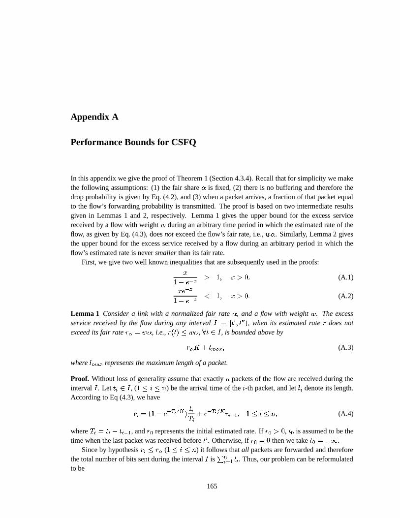
Appendix A

Performance Bounds for CSFQ

In this appendix we give the proof of Theorem 1 (Section 4.3.4). Recall that for simplicity we makethe following assumptions: (1) the fair share � is fixed, (2) there is no buffering and therefore thedrop probability is given by Eq. (4.2), and (3) when a packet arrives, a fraction of that packet equalto the flow’s forwarding probability is transmitted. The proof is based on two intermediate resultsgiven in Lemmas 1 and 2, respectively. Lemma 1 gives the upper bound for the excess servicereceived by a flow with weight � during an arbitrary time period in which the estimated rate of theflow, as given by Eq. (4.3), does not exceed the flow’s fair rate, i.e., � � . Similarly, Lemma 2 givesthe upper bound for the excess service received by a flow during an arbitrary period in which theflow’s estimated rate is never smaller than its fair rate.

First, we give two well known inequalities that are subsequently used in the proofs:

��� ' ; � � � � � ���

(A.1)

�(' ; �

�� ' ; ��

� � � � � (A.2)

Lemma 1 Consider a link with a normalized fair rate � , and a flow with weight � . The excessservice received by the flow during any interval � � � �� � � � , when its estimated rate � does notexceed its fair rate � � � � � , i.e., � � � � � � � ,

� ��� , is bounded above by

� � � � � ����� � (A.3)

where � � � � represents the maximum length of a packet.

Proof. Without loss of generality assume that exactly � packets of the flow are received during theinterval � . Let �

��� , ( � � � � ) be the arrival time of the � -th packet, and let �

denote its length.

According to Eq (4.3), we have

�

� ��� ' ; �� � �

� ' ; �� �

;>=

� � � � � � (A.4)

where � �

� � ;>= , and ��

represents the initial estimated rate. If �� � �

, ��

is assumed to be thetime when the last packet was received before � . Otherwise, if �

�� �

then we take ��� ��� .

Since by hypothesis �

� � � ( � � � � ) it follows that all packets are forwarded and therefore

the total number of bits sent during the interval � is ��� = �

. Thus, our problem can be reformulated

to be

165

������ � � = �

��

(A.5)

subject to

�

� � �

� � � � � � (A.6)

From Eq. (A.4) it follows that

�� �

� � ;>= ' ; �� � ' ; �� � � � � � � � (A.7)

The above equation does not apply for � � , since it is not well defined for the case in which��� �

. Recall that in this case we take ��� ��� , and therefore = � � . Further, define

8 � � =� � � � � � � � �

�� �

�� � �

� (A.8)

Our goal then is to maximize 8 � � =� � � � � � � � �

�� . By plugging �

from Eq. (A.7) into 8 � � =

� � � � � � � � ���

and taking the derivate with respect to �

( � � � � � ) we obtain

�8 � � =

� � � � � � � � ���

��

�

�� ' ; �� �

�= ' ;

� � ��

�� ' ; � � �� � � � ��� � (A.9)

and�8 � � =

� � � � � � � � ���

��� � �

�� ' ; � �� � (A.10)

By using Eqs. (A.1) and (A.2) (and after making substitutions � � = � ,

�= � � � � , and � � � � ) we have

�8 � � =

� � � � � � � � ���

��

� ��� � � � � � � (A.11)

Thus, 8 � � =� � � � � � � � �

�� is maximized when � � � � � � � � � �

�achieve their maximum value, which in

our case is � � . Consequently, we have

8 � � =� � � � � � � � �

�� �

�� � �

(A.12)

�

�� ��

� � ;>= ' ; �� �� ' ; ��

� � � � � = '#;�� �� �� ' ; � �� � �� � � � � � � '�; �� � ' ; ��

� � � � � = ' ;�� �� �� ' ;�� �� � � � ���

� � � � � � = � '�;����

�� ' ;�� �� � � � � � � � ���

�

� � � � � �� � �

� � � � � � � � � � � � �

166

where the next to last inequality follows from the fact that � =� �

, � � � � � , and by using Eq. (A.2)after substitution � � � � .

By using Eq. (A.12), and the fact that � = � � ����� , we get�� = �

� � = � 8 � � =

� � � � � � � � ����� ��� � � � � � � � � � � � � � � (A.13)

Since � � �)� �&� � represents exactly the service to which the flow is entitled during the interval � , itfollows that the excess service is bounded by � ����� � � � � .

Lemma 2 Consider a link with a normalized fair rate � , and a flow with weight � that sends at arate no larger than

�, where

� � � � . Next consider an interval � � � � � � � such that � representsthe time just after a packet has arrived, and during which the rate estimator � is never smaller than� � � � � , i.e., � � � � � � � ,

� ��� . Then, the excess service received by the flow during � is bounded

above by

� � � ln�

� � (A.14)

Proof. Again, assume that during the interval � the flow sends exactly � packets. Similarly, let �

be

the arrival time of the � -th packet, and let �

denote its length. Since we assume that when the packet� arrives, a fraction of that packet equal to flow � ’s forwarding probability, i.e., � � ���

is transmitted,the problem reduces to find an upper bound for�

� = �

� ��

�(A.15)

where � �� �

� � � � � � � .

From Eq. (A.4), we obtain

��

� �

� � ;>= '�; �� �

��� ' ; �� �

(A.16)

� � �

� �

;>=�

� '�; ��

� ' ; �� � � � � � �

Note that unlike Eq. (A.7), the above equation also applies for � � . This because we areguaranteed that there is at least one packet received before � and therefore = is well defined, i.e.,from the hypothesis we have = � � = � � � � � = � � .

Further, by making substitution � � � � in Eq. (A.2) we have

'�; ��

�� ' ; �� �

� � � � � (A.17)

From the above inequality and Eq. (A.16) we obtain

��

� � �

�� �

;>=�

�� � � � � � � (A.18)

and further

167

� � =

��

�

�� =

� �

�� =

��� �

;>=�

�� � � � � � � �

� � =

� � �

;>=�

�� (A.19)

Next, since the arithmetic mean is no smaller than the geometric mean, i.e., � ��� = �

� � � �

����� = �

� =��, where �

� �

( � � � � ), we have�� =

��� �

;>=�

�� � �

� � =�

;>=�

� � � �

� ��� =�

;>=�

� = ��

(A.20)

� �� � � � �

�� � = �

� �� �

��� � � �� � = � � � �

where the last inequality follows from the hypothesis, i.e., � �� �

� �

(� � � � � ).

By replacing � � � � ��� � � = ��

in the well known inequality ln ��� � � � �� � , ( � � ), we obtain� ��� � � � � � � = �

���

ln � � ��� � � , � � . Thus, Eq. (A.19) becomes�� =

��� �

;>=�

� �ln�

� �� (A.21)

Finally, from Eqs. (A.19) and (A.21) we obtain�� = �

� ��

� � � � � � � ��� � � �

�� =

��� �

;>=�

�(A.22)�

� � � � � � ��� � � � ln�

� �Since � � � � �&� � represents exactly the number of bits that the flow is entitled to send during theinterval � , the proof follows.

Theorem 1 Consider a link with a normalized fair rate � , and a flow with weight � . Then, theexcess service received by a flow with weight � , that sends at a rate no larger than

�, is bounded

above by

� � �� � ln

�

� �

� � ��� � � (A.23)

where � � � � � , and � � � � represents the maximum length of the packet.

Proof. Assume the flow becomes active for the first time at � � . Let ��

be the time when its rateestimator exceeds for the first time � � , i.e., � � � � � � � � and � � � � � � � ,

�

�� � . If such a time

� � does not exist, according to Lemma 1, the excess service received by the flow is bounded by� � � � � ��� � , which concludes the proof for this case. In the following paragraphs, we consider thecase when �

�exists.

Next, we show that the service received by the flow is maximized when � � � � � � � ,��� � � . The

proof is by contradiction. Assume there is an interval � :� � � � � ��� � , such that � � � � , and that� � � �

�� � , ( � � �

�� ). Then using an identical argument as in Lemma 1, it can be shown that the

168

service that the flow receives during � increases when � � � � � � � ,� � � . The only change in the

proof of Lemma 1 is that now Eq. (A.7) will also apply for � � , as according to the hypothesisthe estimated rate just before �� (i.e., �

�in Lemma 1) is greater than zero; more precisely �

� �� � .

Further, by including � = in the definition of 8 ��� � (see Eq. (A.8)) we show that 8 ��� � is increasing ineach of its arguments �

, � � � � .

Thus, the service received by the flow is maximized when the estimated rate of the flow is nosmaller than � � after time �

�. But then, according to Lemma 2, the excess service received by the

flow after ��

is bounded by 1

� � � ln�

� �� (A.24)

Similarly, from Lemma 1 it follows that the excess service received by the flow during theinterval � � � � � � � is bounded above by

� � � � � ����� � (A.25)

and therefore by combining (A.24) and (A.25) the total excess service is bounded above by

� � �� � ln

�

� �

� � � � � � � (A.26)

1Without loss of generality here we assume that ��� represents the time just after � was evaluated as being smaller than

� � for the last time. Since this coincides with a packet arrival Lemma 2 applies.

169

170

Appendix B

Performance Bounds for Guaranteed Services

B.1 Network Utilization of Premium Service in Diffserv Networks

Premium service provides the equivalent of a dedicated link of fixed bandwidth between edge nodesin a Diffserv network. In such a service, each premium flow has a reserved peak rate. In the dataplane, ingress nodes police each premium service traffic flow according to its peak reservation rate.Inside the Diffserv domain, core routers put the aggregate of all premium traffic into one schedulingqueue and service the premium traffic with strict priority over best effort traffic. In the controlplane, a bandwidth broker is used to perform admission control. The idea is that by using veryconservative admission control algorithms based on worst case analysis, together with peak ratepolicing at ingress nodes and static priority scheduling at core nodes, it is possible to ensure that allpremium service packets incur very small queueing delay.

One important design question to ask is how conservative does the admission control algorithmneed to be? In other words, what is the upper limit on the utilization of the network capacity that canbe allocated to premium traffic if we want the premium service to achieve the same level of serviceassurance as the guaranteed service, such that the queueing delay of all premium service packets isbounded by a fixed number even in the worst case?

For the purpose of this discussion, we use flow to refer to a subset of packets that traverse thesame path inside a Diffserv domain between two edge nodes. Thus, with the highest level of trafficaggregation, a flow consists of all packets between the same pair of ingress and egress nodes. Notethat even in this case, the number of flows in a network can be quite large as this number mayincrease quadratically with the number of edge nodes.

Let us consider a domain consisting of ��� routers with links of capacity � . Assume that

the fraction of the link capacity allocated to the premium traffic is limited to . Assume also thatall flows have equal packet sizes, and that each ingress node shapes not only each flow, but alsothe aggregate traffic at each of its outputs. Figure B.1(a) shows the traffic pattern at the first corerouter along a path. Each input receives 12 identical flows, where each flow has a reservation of � � �)� � � � � . Let � be the transmission time of one packet, then as shown in the Figure, theinter-arrival time between two consecutive packets in the each flow is � ��� , and the inter-arrival timebetween two consecutive packets in the aggregate flow is � � .

Assume the first three flows at each input are forwarded to output 1. This will cause a burstof 12 packets to arrive at output 1 in a ��� long interval and the last packet of the burst to incuran additional delay of ��� . Now assume that the next router receives at each input a traffic pattern

171

...

11

2

3

4

1

2

3

4

1

...

...

...

...

11

14567891011 23121

...

...

...

...

...

...

...

delay = 3

...delay = 9...

...

...

2

a)

b)

8

2

3

4

1

2

3

4

1

Figure B.1: Per-hop worst-case delay experienced by premium traffic in a Diffserv domain. (a) and (b) showthe traffic pattern at the first and a subsequent node. The black and all dark grey packets go to the first output;the light grey packets go to the other outputs.

similar to the one generated by output 1 of the first core router, as shown in Figure B.1(b). Inaddition, assume that the last three flows from each input burst are forwarded to output 1. This willcause a burst of 12 packets to arrive 1 at output in a ��� long interval and the last packet in the burstto incur an additional delay of ��� . Thus, after two hops, a packet is delayed by as much as ��� .This pattern can be repeated for all subsequent hops.

In general, consider a��

�router, and let � be the number of flows that traverse each link. For

simplicity, assume that � �� � . Then it can be shown that the worst case delay experienced by apacket after � hops is

� ��� � �� � � � �

� �� � � � � �� �

� � � � � � � � (B.1)

where the first term is the additional delay at the first hop, the second term is the additional delay atall subsequent hops, and the last term accounts for the packet transmission time at each hop. As aa numerical example, let ��� Gbps, a packet size of 1500 bytes,

�� � , � � � , � � � � �

and �,� � . From here we obtain � � � � sec, and a delay�

of over 240 ms. Finally, if �

�� � ,it can be shown that it will take only

� � ���� ��� ��� hops to achieve a continuous burst. For example,

for �� �� and�� � , it takes only two hops to obtain a continuous burst.

The above example demonstrates that low network utilization and traffic shaping at ingressnodes alone are not enough to guarantee a “small” worst-case delay for all the premium traffic. Thisresult is not surprising. Even using a per flow scheduler like Weighted Fair Queueing (WFQ), willnot help to reduce the worst case end-to-end delay for all packets. In fact, if all flows in the aboveexample are given the same weight, the worst case delay under WFQ is � � � , which is basically thesame as the one given by Eq. (B.1). However, the major advantage of using WFQ is that it allows usto differentiate among flows, which is a critical property as long as we cannot guarantee a “small”delay to all flows. In addition, WFQ can achieve 100% utilization.

172

B.2 Proof of Theorem 2

In this appendix we show that a network of CJVC servers provides the same end-to-end delayguarantees as a network of Jitter-VC servers. In particular, in Theorem 2 we show that the deadlineof a packet at the last hop in both systems is the same. This result is based on Lemmas 4 and 5which give the expressions of the deadline of a packet at the last hop in a network of Jitter-VC,and a network of CJVC servers, respectively. First, we present a preliminary result used in provingLemma 4.

Lemma 3 Consider a network of Jitter-VC servers. Let � � denote the propagation delay betweenhops � and � � , and let � � be the maximum transmission time of a packet at node � . Then for any��� and � � � � we have

� �� � � = � � �

� � ��� � � � � � � �

� � � � �

� � ;>= ��� � ;>= � � � ;>= � (B.2)

Proof. The proof is by induction on�

. First, recall that by definition �� � �

� �� � � � � � � �

� � (see

Table 5.1), and that for � � , � �� � � � �

� � ;>= � � � ;>= . From here and from Eqs. (5.1) and (5.2) we

have then

� �� � � � ��� � � �

� � � �

� � ;>=

� � ��;>=� � � � � �

�

� ����� � � �

� � ;>= � � � ;>= ��� � ;>= � � ��;>=

� � � � � �

�

� (B.3)

Basic Step. For�� and any � � , from Eq. (B.3) we have trivially

� =

� � �

� =

� � ;>= � � � ;>= � � � ;>= ��&=

���, ��� , and therefore

�=

� � � � =

� � ;>= � � � ;>= � � � ;>= � �&=

���, � � .

Induction Step. Assume Eq. (B.2) is true for�

. Then we need to show that

� ��=

� � � = � � � � =

� � � � � � � � � � �

�=

� � � � � � =

� � ;>= � � � ;>= � � � ;>= ������ � � � � =� � � � � ��� � � � �

� � � = � � ����� � � � � =

� � ;>= � � � ;>= ��� � ;>= � � �

� � � � � � � � � � (B.4)����� � � � � =

� � ;>= � � � ;>= ��� � ;>= � � �

� � � � ����� � � � � =

� � ; � � � � ; � ��� � ; � � � �

� � ;>= � � � � ;>= � � � ;>= �

where the second inequality follows after using Eq. (B.3). Next consider two cases: whether� ��=

� � ;>= �

� � ;>= � � � ;>= � � �� � or not. Assume

� ��=

� � ;>= � � � ;>= � � � ;>= � � �

� � . From Eq. (B.4) and from the

induction hypothesis we obtain� ��=

� � � = � � � � =

� � � � � � � � � ����� � � � � =

� � � � � ��� � � � �

� � � = � � (B.5)����� � � � � =

� � ;>= � � � ;>= � � � ;>= � � �

� � � � � � � � �

� ����� � � � � =� � � � � ��� � � � �

� � � = � � � �

� � � � � � � �� � �

� � � = � � �

� � � � � � � � (induction hypothesis)

� � �� � � � �

� � ;>= � � � ;>= � � � ;>=� � �

� � � ����� � � � � =

� � ; � � � � ;>= ��� � ;>= � � �

� � ;>= � � � � ;>= � � � ;>=

� ����� � � � � =� � ;>= � � � ;>= � � � ;>= � � �

� � � ������ � � � � =

� � ; � � � � ; � � � � ; � � � �

� � ;>= � � � � ;>= � � � ;>=

�� ��=

� � � � � � =

� � ;>= ��� � ;>= � � � ;>= �173

Next, assume that� ��=

� � ;>= � � � ;>= � � � ;>= � � �

� � � (B.6)

From here and by using Eq. (B.3) and Eq. (B.4) we have

� ��=

� � � = � � � � =

� � � � � � � � � � ��� � � � � =

� � � � � ��� � � � �

� � � = � � (B.7)� ��� � � � � =

� � ;>= � � � ;>= ��� � ;>= � � �

� � � � � � � � �

� � ��� � � � � =� � � � � ��� � � � �

� � � = � � � � � =

� � ;>= � � � ;>= � � � ;>= � � � � � �� � �

�=

� � � � � � =

� � ;>= � � � ;>= � � � ;>=�

� ��=

� � � ����� � � � � =

� � ;>= � � � ;>= ��� � ;>= � � �

� � � (Eq. (B.3))

� � � � =�

(Eq. (B.3))

�� ��=

� � ;>= � ����� � � � � =

� � ; � � � � ; � ��� � ; � � � �

� � ;>= �

� � ��� � � � � =� � ;>= � � � ;>= ��� � ;>= � � �

� � � � � � ;>= � � � ;>= � (Eq. (B.6))� ��� � � � � =

� � ; � � � � ; � ��� � ; � � � �

� � ;>= �

�� ��=

� � � � � � =

� � ;>= � � � ;>= � � � ;>= �This completes the proof.

Lemma 4 The deadline of any packet � �,� � , at the last hop � in a network of Jitter-VC servers

is

� �� � � � ���

�' �� = � � ���

�

��;>=

� � = � � � ��� � � � � ��;>=� � � ���

�

�� (B.8)

Proof. Let ��� � be the last hop for which� �� � � ;>= � � � � ;>= � � � � ;>=

�� ��;>=� � � . We consider two

cases whether � � exists or not.

Case 1. (��� does not exist) From Eq. (5.1) we have ' �� � �

� �� � ;>= � � � ;>= � � � ;>= , � � . From here

and by using Eq. (5.2) we obtain

� �� � � ' �

� = � � ���

�

��;>=

� � = � � � ��� � � � (B.9)

Because we assume that ��� does not exist we also have� �� � � ' �

� � � ���

���� � ��;>=

� � � ���

���, which

concludes the proof of this case.

Case 2. (� � exists) In this case we show that � � � � . Assume this is not true. Then we have' �� � �

� �� � ;>= � � � ;>= ��� � ;>= , � � ��� . By using Eq. (5.2) we obtain

� �� � � ' �

� � � � � � � � � � �� � �

�

��;>=

� � � � � �� ��� � � � (B.10)

174

On the other hand, by the definition of ��� and from Eqs. (5.1) and (5.2) we have

� �� � � � ����� � � �

� � � ;>= � � � � ;>= � � � � ;>= � � ��;>=

� � � � � ���

�

(B.11)

� � �� � � ;>= � � � � ;>= ��� � � ;>= � ���

�

�

As a result we obtain� �� � � � � �

� � � ;>= � � � � ;>= � � � � ;>= � �

���. By iteratively applying Lemma 3 we

have

� �� � � = � � �

� � � � � � � � � � �

� � � � � �

� � � ;>= � � � � ;>= � � � � ;>= � � �

�

� � � � � (B.12)

From Eq. (B.12) we obtain

�;>=

� � � � �� �� � � = � � �

� � � � � � � � � � � � � � � � � � �

� � � � � �

� � � ;>= � � � � ;>= � � � � ;>= � (B.13)

� � � � � � � ����

�where the right-hand term can be expressed as

�;>=

� � � � �� �� � � = � � �

� � � � � � � � � � � �

� � � � �

� � � �

�;>=

� � � � � �� ��� � � � (B.14)

By combining Eq. (B.13) and Eq. (B.14) we get

� �� � � � �

� � � � � � � � � � � �

�

��;>=

� � � � � �� ��� � � (B.15)

� ' �� � � � � � � � � � �� ���

�

��;>=

� � � � � �� ��� � � �

But this inequality contradicts Eq. (B.10) and therefore proves our statement, i.e., � � � � . Thus,' �� � �

� ��;>=� � . From here and from Eqs. (5.1) and (5.2) we get

� �� � � ' �

� � � �

�

�� ��;>=� � � �

�

� (B.16)

Now, from Eq. (5.1) it follows trivially that

' �� � � � ��� � � �

� � ;>= � � � ;>= ��� � ;>= � � �

� � ;>= �

� � �� � ;>= � � � ;>= ��� � ;>= � � � �� (B.17)

By iterating over the above equation and then using Eq. (5.2) we get

� �� ��' �� = � � � �

�

��;>=

� � = � � � ��� � � � (B.18)

which, together with Eq. (B.16), lead us to Eq. (B.8).This completes the proof of the lemma.

175

Lemma 5 The deadline of any packet � �,� � , at the last hop � in a network of CJVC servers is

� �� � � � ���

�' �� = � � � �

�

��;>=

� � = � �� ��� � � � � ��;>=

� � � � �

�

�� (B.19)

Proof. We consider two cases whether � �� �

or not.

Case 1. ( � �� �

) From Eqs. (5.2) and (5.6) it follows that

� �� � � ' �

� = � � � �

�

��;>=

� � = � � � ��� � � � (B.20)

On the other hand, by the definition of � �

(see Eq. (5.3) and Eq. (5.4)) we have ' �� � �

� �� � ;>= �

� � ;>= ��� � ;>= � � �� � ��;>=

� � ,

� � . From here and from Eq. (5.2) we obtain

� �� �� � ��;>=

� � � � �

�

� (B.21)

From this inequality and Eq. (B.20), Eq. (B.19) follows.

Case 2. ( � �� �

) By using Eqs. (5.2) and (5.10) we obtain

� �� � � ' �

� = � � � �

�

� � � � �� � ��

�;>=

� � = � � � ��� � � (B.22)

� ' �� = � � � �

�

� � � � � �� � ��;>=

� � � � �� � ��;>= � � �

�

� ' � � = � ' ��;>=� = � � ��;>=

�

��;>=

� � = � � � ��� � �� ' ��;>=

� = � � � ��;>=

�

� � � � �� � ��;>=

��;>=

� � = � �� ��� � � � ���

�

�� ��;>=� � � � �

�

�

Since � �� �

, by using again Eq. (5.2) and (5.7) we get

� �� � � ' �

� = � � ���

�

� � � � �� � ��

�;>=

� � = � � � ��� � � (B.23)

� ' �� = � � � �

�

��;>=

� � = � � � ��� � � �which, together with Eq. (B.22), lead to Eq. (B.19).

Theorem 2 The deadlines of a packet at the last hop in a network of CJVC servers is equal to thedeadline of the same packet in a corresponding network of Jitter-VC servers.

176

Proof. From Eqs (5.1) and (5.2) it is easy to see that in a network of Jitter-VC servers we have

� =� � � ' =

� = � � � �

�

��;>=

� � = � �� ��� � � � (B.24)

Similarly, in a network of CJVC servers, from Eqs. (5.1) and (5.7), and by using the fact that� =� �

(see Eq. 5.8), we obtain an identical expression for� =� � (i.e., Eq. (B.24)).

Finally, since (a) the eligible times of all packets � �

at the first hop, i.e., ' �� = (

� � ), areidentical for both Jitter-VC and CJVC servers, and since (b) the deadlines of the packets at the lasthop, i.e.,

� �� � ( � � ), are computed based on the same formulae (see Eqs. (B.8), (B.19) and B.24),

it follows that� �� � , (

� � ) are identical in both a network of Jitter-VC, and a network of CJVCservers.

B.3 Proof of Theorem 3

To prove Theorem 3 (see Section 5.3.3) we prove two intermediate results: Lemma 9 which givesthe buffer occupancy for the case when all flows have identical rates, and Lemma 12 which givesthe buffer occupancy for arbitrary flow rates.

B.3.1 Identical Flow Rates

Consider a work-conserving server with an output rate of one, which is traversed by � flows withidentical reservations of �� � . Assume that the time axis is divided in unit sized slots, where slot �corresponds to the time interval � � � ��� �� . Assume that at most one packet can be sent during eachslot, i.e., the packet transmission time is one time unit. Finally, assume that the starting times ofthe backlogged periods of any two flows are uncorrelated. In practice, we enforce this by delayingthe first packet of a backlogged period by an amount drawn from a uniform distribution in therange � � � � �

� � �

� � � � �

� � � � ��� , where � � � �

� � � is the arrival time of the first packet in the backlogged

period. Note that according to Eq. (5.1), the eligible times of the packets of a flow during a flow’sbacklogged interval are periodic with period � . Thus, without loss of generality, we assume that thearrival process of any flow during a backlogged interval is periodic.

Let � � � � � � denote the number of packets received (i.e., became eligible) during the interval� � � � � , and let � � � � � � denote the number of packets sent during the same interval. Note that� � � � � � and � � � � � � do not include packets received/transmitted during slot � . Let � � � � denote thesize of the queue at the beginning of slot � . Then, if no packets are dropped, we have

� � � � � � � � � � � � � � � � � � � � � � � � (B.25)

Since at most one packet is sent during each time slot, we have � � � � � � � � � � . The inequalityholds when � � � � � belongs to a server busy period. A busy period is defined as an interval duringwhich the server’s queue is never empty. Also, note that if � is the starting time of a busy period� � � � � �

.The next result shows that to compute an upper bound for � � � � , it is enough to consider only the

scenarios in which all flows are continuously backlogged.

177

Lemma 6 Let � = be an arbitrary time slot during a server busy period that starts at time ��. Assume

flow � is not continuously backlogged during the interval � � � � � = � . Then � � � = � can only increase ifflow � becomes continuously backlogged during � � � � � = � .Proof. Consider two cases in which flow � is idle during the entire interval � � � � � = � , and not.

If flow � is idle during � � � � � = � , consider the modified scenario in which flow � becomes back-logged at an arbitrary time �

���, and remains continuously backlogged during � � � � � = � . In addition,

assume that the arrival patterns of all the other flows remain unchanged. As a result, it is easy tosee that in the modified scenario, the total number of packets received during � � � � � = � can only in-crease, while the starting time of the busy interval can only decrease. Let � , � , and � denote thecorresponding values in the modified scenario. Then � � � � � � � � � � � � �

, � � � � � � = ��� � � � � � = � , and

� � � � � � = � � � � � � � � = � � � = � � � . From Eq. (B.25) it follows then that � � � = ��

� � � = � .In the second case, when flow � is neither idle nor continuously backlogged during the interval� � � � � = � , let � denote the time when the last packet of flow � arrives during � � � � � = � . Next consider the

modified scenario in which flow � ’s packets arrive at times: � � � � � � � � � � ��� � � � � � � � � � � � � � � � ,such that � � � � � �

�, and � =

� � � � � . It is easy to see then that the number of packets of flow� that arrive during � � � � � = � is no smaller than the number of packets of flow � that arrive during thesame interval in the original scenario. By assuming that the arrival patterns of all the other flowsdo not change, it follows that � � � � � � = �

�� � � � � � = � . In addition, since at most � = � � � packets are

transmitted during � � � � � = � we have � � � � � � = �� � = � � � . The inequality holds if, after changing the

arrival pattern of flow � , the server is no longer busy during the entire interval � � � � � = � . In addition,we have � � � � � � �

, and from the hypothesis � � � � �)� �. Finally, from Eq. (B.25) we obtain

� � � = ��

� � � = � , which concludes the proof of the lemma.As a consequence, in the remainder of this section, we limit our study to a busy period in which

all flows are continuously backlogged.Let � = be the time when the last flow becomes backlogged. Let �

�be the latest time no larger than

� = when the server become busy, i.e., it has no packet to send during � � � � � � � � and is continuouslybusy during the interval � � � � � = � �� . Then we have the following result.

Lemma 7 If all flows remain continuously backlogged after time � = , the server is busy for any time����.

Proof. By the definition of ��, the server is busy during � � � � � = � . Next we show that the server is also

busy for any � =� �

.Consider a flow that becomes backlogged at time � , Since its arrival process is periodic it follows

that during any interval � �� � � � � � � � � � , � � �, exactly one packet of this flow arrives. Since

after time � = all � flows are backlogged, exactly � packets are received during � � = � � � � � � = � � � , ��� �. Since at most � packets are sent during each of these intervals, it follows that the server

cannot be idle during any slot � .Consider a buffer of size � . Our goal is to compute the probability that the buffer will overflow

during an arbitrary interval � � � � � � � � � . From Lemma 7 it follows that since the server is busy during� � � � � � � � � , exactly�

packets are transmitted during this interval. In addition, since the starting timesof the backlogged periods of different flows are not correlated, in the remainder of this section wealso assume that the starting times of a flow’s backlogged period is not correlated with the starting

178

time, ��, of a busy period. Thus, during the interval � � � � � � � � � , a flow receives

� � � � � packets withprobability � � � � � � � � � � � � ��� , and

� � � ��� with probability � � . Since this probability is periodicwith period � it will suffice to consider only intervals of size equal to at most � . Consequently, wewill assume

� � � . The probability to receive one packet during � � � � � � � � � is then

� � � � ��

� � (B.26)

Let � � � �� � denote the probability with which exactly

�

packets are received during the timeinterval � � � � � � � � � , where

� � � �� � �

� ��

�� � � � � ����� � � � �

�; � � (B.27)

Now, let� ��� � �

� � � denote the probability with which the queue size exceeds � at time �� � � .

Since the server is idle at ��

and busy during � � � � � � � � � , from Eq. (B.25), it follows that the server’squeue overflows when more than � � � packets are received during � � � � � � � � � . Thus, we have

� ��� � �� � � �

�

� � ��� � = � � � � � � ��

� � ��� � =� � ��� ��� �

����� ��� � �

�;

� (B.28)

The next result computes� ��� � �

� � � .Lemma 8 The probability that a queue of size � overflows at time �

� � � is bounded by

� ��� � �� � �

� ������

� � �

� � ����� �� ��� � � ����� �� ��� �

� � � ��� � � � �� ��� � (B.29)

where

������ � ������' � = � � = � = �

��.

Proof. From Eq. (B.27) we obtain

� � � � � � � � � ��� � ��� ��� � � � � �

� � � � � � � � � � (B.30)

By plugging the above equation and Eq. (B.26) into Eq. (B.28) we obtain

� ��� � �� � � � � ��� � � � � �

�

� � ��� � =��

;>=�

� � � ��� � � �� � �� � �

� � ��; � ;

�(B.31)

�� ��� � � � � �

�

� � ��� � =��

;>=�

� � � ��� � ��� � �

� � � � � �� ���

�; � ;

�� � ��� � � � � �

�

� � ��� � = � � � � � �

��� �� �� � �

�; � ;

�Next, it can be easily verified that for any positive reals � ,

�, and � , such that

� � � � �, we have

�� � � �

� � ��

�� � � � � �� � � � �

� �� (B.32)

179

By taking �0� � ,�� � � � , ��� � , Eq. (B.31) becomes

� ��� � �� � �

�� ��� � � � � �

�

� � ��� � = � � � �

��� �

� � �; � ;

� � �� ��� � � � � ��� � �

� � � �

� � �

� �(B.33)�

� ��� � � � � � ��� � � � �� � � �

Next, it remains to bound � ��� � � � � � . From Eqs. (B.26) and (B.30) we have

� ��� � � � � � � � ��� � � ��;>=�� �

� �� � � � � � � � �

� � � � � � �

;>=�� �

� �� � � � � � � � �

� ����� (B.34)

By using Eq. (B.32) with �0� � ,�� � � � , and ����� , we obtain

� ����� � � � � � � ��� � � ��;>=�� �

� � � �� � �

� �� � ��� � � �

�;>=�� �

� � � �� � � � � � � � �� �

� � ��� �� ��� (B.35)

Again, by applying Eq. (B.32) to the pairs ��� � � � � ��� � � � and ��� � � � � � � � ��� � � � � � � , ��

� ��� , we have

� ��� � � � � ��� ��� � � �

� � � � ��� � ��� � � ��� � ��

� � �� � ��� � � �

� � ��� � �� ��� � � ��� � �� ��� �

� � �� (B.36)

To bound � ��� � � � we use Stirling inequalities [26], i.e.,� � � � ������' �

� ����

�� � � � ������' �

� � �=�= ���, � � . From here we have

� �� � �

� � � � � � ������' �� � �

=�= ���

� � � � ��� ��' � � � � � ��� � � � � ��� � � � ��' ��; �

(B.37)

�� �� � ��� � � � � � �

�������' � = � = �

�� � ��� � � �

�; ��

By combining Eqs. (B.26), (B.27) and (B.37), we obtain

� ��� � � �� �

������ �� � � ��� � � �

�������

� � � � (B.38)

where

������ � ������' � = � � = � = �

��

and the last inequality follows from the fact that ��� � ��� ��� � � ��

,for any � � , � � � . By plugging the above result in Eq. (B.33) we obtain

� ��� � �� � �

� ������

� � �

� � ��� � �� ��� � � ��� � �� ��� �

� � � ��� � � � �� ��� � (B.39)

180

Lemma 9 Consider � flows with identical rates and unit packet sizes. Then given a buffer of size� , where

����� � � �

� � � � �� �

� �(B.40)

the probability that the buffer overflows during an arbitrary time slot when the server is busy isasymptotically

� � .Proof. To compute the asymptotic bound for

� ��� � �� � � assume that ��� � . Since � � � � � � �

� � � � � � and� � � � � � � � , for � �

�, and since ��� � � � � � � �

�� for � � �

� � , and������

��� � � for any � � , by using Eq. (B.29) we obtain1

� � � ��� � �� � � �

� � � � ����� � � ��� � � � � � � � ��� � �� ��� �

� ��� � �� ��� �� � � � � � � � � (B.41)

�� � � � ����� �

� ��� � � � � � �

� ��� �

� � � � � � � � ��

� � � � ����� � � �� � � � � �

� � � � � � � � �� � � � � � ����� ��� � � � � � � � � �� � �

� � � � � � �Using � to bound

� ��� � �� � � leads us to

� ��� � � � � � � � � (B.42)

�� � � � �

��� � � � � � � � �

����� � � �

� � � � �� �

��

Next we prove a stronger result by computing an asymptotic upper bound for the probabilitywith which a queue of size � overflows during an arbitrary busy interval. Let ����� � � � denote thisprobability. The key observation is that since all flows have period � , the aggregate arrival trafficwill have the same period � . In addition, since during each of these periods exactly � packets arereceived/transmitted it follows that the queue size at any time �

� � � � � � � is the same, � � � � �

.Consequently, if the queue does not overflow during � � � � � � � ��� , the queue will not overflow atany other time �

�� = during the same busy period. Thus, the problem reduces to compute the

probability of queue overflowing during the interval � � � � � � � ��� . Then we have the following result.

Corollary 1 Consider � flows with identical rates and unit packet sizes. Then given a buffer of size� , where

���� � � � � � � � � � � � ��� � �� � (B.43)

the probability that the buffer overflows during an arbitrary busy interval is asymptotically

� � .1More precisely ��� � �� � � " � ��� � � ����� � � � � � " � � � � � .

181

Proof. Let � be the probability that a buffer of size � overflows at an instant � during the busyinterval � � � � � � � � � . Then the probability that the buffer overflows during this interval is smallerthan � � � � � � �

� � � . Now, recall that if the buffer does not overflow during � � � � � � � ��� ,the buffer will not overflow after time �

� � � . Thus the probability that the buffer will not overflowduring an arbitrary busy period is less than � � . Finally, let � � � � � , and apply the result ofLemma 9 for � , i.e.,

����� � � �

� � � � � � � ���� �

��

��� � � � � � � �

� � �� (B.44)

B.3.2 Arbitrary Flow Rates

In this section we determine the buffer bound for a system in which packets are of unit size, but thereservations can be arbitrary. The basic idea is to use a succession of transformations to reduce theproblem to the case in which the probabilities associated to the flows can take, at most, three distinctvalues, and then to apply the results from the previous case when all reservations are assumed to beidentical.

Consider � flows, and let � � denote the rate reserved by flow�

, where�� � = � � � �� (B.45)

Consider again the case when all flows are continuously backlogged. Let ��

denote the startingtime of a busy period. Since the time when flow

�becomes backlogged is assumed to be independent

of ��, it follows that during the interval � � � � � � � � � flow

�receives exactly

� � � � � � � packets withprobability

� � �� � � � � � � � � � � � � � � (B.46)

and� � � � � � packets with probability ��� � � � � .

Let � � � �� � denote the probability with which the server receives exactly �

�� � = � � �#� � � � �

packets during the interval � � � � � � � � � . Then

� � � �� � �� �� �-� = �

� � � � � � � � � � � � � ��� � � � � (B.47)

where �� �-� = �� � � � � � � � � � � � � �

�� � � � is the coefficient of � � in the expansion of�

�� = ��� �

� � � � ��� � � � � � � � (B.48)

Note that when all flows have equal reservations, i.e., � � � �� � � � � � � , Eq. (B.47) reduces toEq. (B.27).

By using Eq. (B.46) the number of packets received during � � � � � � � � � can be written as�� � =

� � � � � � � � �

�� � = �

� � � � ��� � � � � � � � �� �

�� � = � � �

� � � � � (B.49)

182

Since ��

is the starting time of the busy period and since the server remains busy during � � � � � � � � � ,from Eq. (B.25) it follows that � � � � � � � � � � �

�� � = � � � � � .

Similarly, the probability� ��� � �

� � � will overflow a queue of size � at time �� � � is

� ��� � �� � � �

�� � � = � � � � � �

�(B.50)

where � ����� � = � � ��� � � � .

Since in the following, � � ��� � is always defined over � � � � � � � � � we will drop the argument fromthe � � ��� � ’s notation. Next, note that for any two flows

�and � , � � � � � � can be rewritten as

� � � � � � � � � � ��� � � �

� ��� �-� � ����� � � � ����� � ��� � � � � � � �� � � ����� � � ��� � � � � � � � �

� � � (B.51)

where � � � ��� � � , represents all terms in �� �-� =

� � � � � � � � ��� that contain � � � � , �-� � � �)� � � � � �

� � ��� � � � � � � represents all terms that contain either � � � � � � � or � � � � ��� � , and � � � � � � � � � � � � � �represents all terms that contain ����� � � ����� � � .

From Eqs. (B.50) and (B.51), the probability a queue of size � will overflow at time �� � � is

then

� ��� � �� � � �

�� � � = � � � � � � (B.52)

� � � � � ��� � � � � �� ��� � �-� � ��� � � � � ��� � � ��� � � ��� � � � � �

� ��� ������ � � ��� � � � ��� � � � � � � ��� �

where � � � � � �� ��� ���

�� � � = � � � � � � � , � � � � � �

� ��� ����� � � = � � � � � � � , and � � � � � �

� ��� ����� � � = � � � � � � � ,

respectively.Our next goal is to reduce the problem of bounding

� ��� � �� � � to the case in which the flows’

probabilities take a limited number of values. This makes it possible to use the results from thehomogeneous reservations case without compromising the bound quality too much. The idea isto iteratively modify the values of the flows’ probabilities, without decreasing

� ��� � �� � � . In

particular, we consider the following simple transformation: select two probabilities � � and � � andupdate them as follows:

� � � � � � � � (B.53)

� � � � � � � �where � is a real value such that

� � � �� � �

� , and the new computed probability

� ��� � �� � � � � � � � ��� � � � � �

� ����� �-� � ����� � � � ����� � ��� � � ��� � � � � �� ����� (B.54)

����� � � � ��� � � ��� � � � � �� ��� �

is greater or equal to� ��� � �

� � � .It is interesting note that performing transformation (B.53) is equivalent to defining a new system

in which the reservations of flows�

and � are changed to � � and � � , respectively, such that � � �� �7�� � � � � �7�� � � , and �� � �� �#�� � � � � �#� � � . There are two observations worth noting about this

183

system. First, by choosing � � � � � � � � � and � � � � � � � � � , we maintain the invariant ��� = �

� .

Second, while in the new system the start time ��

of the busy period may change, this will notinfluence

� ��� � �� � � as this depends only on the length of the interval � � � � � � � � � .

Next, we give the details of our transformation. From Eqs. (B.52), (B.53) and (B.54), after somesimple algebra, we obtain

� ��� � �� � � � � ��� � �

� � � � � �-� � � � � � � ��� � � � � �� ��� � (B.55)

where� � � � � � � � � � � � � � � � � � � � � � � � � � ��� � � � � � � � � � � � (B.56)

Recall that our goal is to choose � such that� ��� � �

� � � � � ��� � � � . Without loss ofgenerality assume that � � � � � . We consider two cases: (1) if � � � � � �

� ��� � �, then � � �

and� �

�� � � � ( �

��

and � �

�� � � � cannot be simultaneously true); (2) if � � � � � �

� ��� � �, then

either � � �and � �

� � � � � , or �

��

and � � �)� � � � .Let � �

�� �� ��

=��

���

, and � � � � � �����

=��

���

, respectively. Consider the following three

subsets, denoted � , � , and�

, where � contains all flows�

such that � � � � � �

, � contains allflows

�such that � � � � ��� � , and

�contains all the other flows. The idea is then to successively

apply the transformation (B.53) on � =� � � � � � � � �

�, until the probabilities of all flows in

�become

equal. In this way we reduce the problem to the case in which the probabilities � � can take at mostthree distinct values: � �

�, � ����� , and ��� , where � � � ��� ,

� � �. Figure B.2 shows the iterative

algorithm that achieves this. Lemmas 10 and 11 prove that by using the algorithm in Figure B.2,� =

� � � � � � � � ��

converge asymptotically to the three values.

while ( � � � � ) do ��� while size of�

is greater than one � �� ������� ���� � � �%� ;� � ������ ��� � � � � ;if ( 4 � � �� � ��� � � )� � � � � � � � � � � ��� ;

else� ��������� � � � � � � � � � � � ;� � � � � �; � � � � �

;if (� � � � � )� � ����� ��� ; � � ��� � ��� ;if (� � � � ��� )� � ����� ��� ; � ����� � ��� ;

Figure B.2: Reducing � ��� ����� � � � � � to three distinct values.

Lemma 10 After an iteration of the algorithm in Figure B.2, either the size of�

decreases by one,or the standard deviation of the probabilities in

�decreases by a factor of at least ��� =��� � � � .

Proof. The first part is trivial; if�

� � � � �� ��� � �

the size of�

decreases by one. For the secondpart, let � denote the average values of probabilities associated to the flows in

�, i.e.,

��� �� � �

� � � � (B.57)

184

The standard deviation associated to the probabilities in�

is

�' � �

� �

�-� � � � � � (B.58)

After averaging probabilities � � and � � , standard deviation � changes to

�' � � �

' � � �� � � � � �� � � � � � �-� � � � � � � �-� � � � � � � �

'�� � �-� � ��� � � �� � (B.59)

Since � � and � � are the lowest, and respectively, the highest probabilities in�

we have �-� � � � � �

�-� � ��� � � � , ��� �. From here and from Eqs. (B.58) and (B.59) we have

�' � �

� �

�-� � � � � � � � � �-� � ��� � � � � � � � � � � ' � � � ' � � � �

'�� � � ' � ����

� � � ���(B.60)

Lemma 11 Consider � flows, and let �

denote the probability associated with flow � . Then, by

using the algorithm in Figure B.2, the probabilities �

( � � � � ) converge to, at most, three

values.

Proof. Let � be an arbitrary small real. The idea is then to show that after a finite number ofiterations of the algorithm in Figure B.2, the standard deviation of �

’s ( � � �

) becomes smallerthan � .

The standard deviation for the probabilities of flows in�

is trivially bounded as follows

�' � �

� �

�-� � � � � �

� ��-� ����� ��� � � � � � � � � �-� ��� � ��� � � � � � � �-� ����� ��� � � � � � (B.61)

Assume�

� � � � �� ��� � �

(i.e.,�

does not change) for � = consecutive iterations. Then, by usingLemma 10, it is easy to see that � = is bounded above by

�, where

�' � �

���

� � � �� � �

�' � �

���

� �� �

� � � � �� � � � � � ' � �� � ��� �� � � ��� � � (B.62)

Since the above bound,�

, holds for any set�

, it follows that after � �iterations, we are guaranteed

that either set�

becomes empty, a case in which the lemma is trivially true, or�'��

� � .Thus, we have reduced the problem to compute an upper bound for probability

� ��� � �� � � in

a system in which probabilities take only three values at time � : � � �

, � � � � , and ��� .Next we give the main result of this section

Lemma 12 Consider � flows with unit packet sizes and arbitrary flow reservations. Then given abuffer of size � , where

���� � � � � �

� � � � �� �

� �(B.63)

the probability that the buffer overflows in an arbitrary time slot during a server busy period isasymptotically

� � .185

Proof. Consider the probability,� ��� � �

� � � , with which the queue overflows at time �� � � (see

Eq. (B.50)). Next, by using the algorithm in Figure B.2, we reduce probabilities �

’s ( � � � � ) to

three values: � � � � � � � � , and � � , respectively. Let � �

denote the final probability of flow � , and let

� � ��� � �� � � denote the final probability of the queue overflowing at time �

� � � . More precisely,from Eqs. (B.50) and (B.47) we have

� � ��� � �� � � �

�� � � = �

� � � � � � ��� � � =

��-� =

� � � � � � � � ��� � (B.64)

where � � ��� � = � � ��� ��� � , and �

� � �

�, � � � , �

� � ��� � ,

� � � , and �

� ��� ,

� � � .Since after each transformation

� ��� � �� � � can only increase, we have

� � ��� � �� � � � � ��� �

�� � � .

Let � � , ��� , and � � be the number of flows in sets � , � , and�

, respectively. Define integers� � , ��� , and � � , such that �0� � � � ��� � � � , and � �

�� � � ���

���� , and � �

�� � , respectively.

Then, it can be shown that

� � ��� � �� � � � � � � � � � � � �

(B.65)

where

� � �

��

� � � � =� � ��

��

�

������ � � �

�� ;

(B.66)

� � �

��

� � � � =� ����

��

� � � ����� ��� � �

�� ;

� � �

��

� � � � =� � ��

��

� ������� �

�� ;

�

Due to the notation complexity we omit the derivation of Eq. (B.65). Instead, below we give analternate method that achieves the same result.

The key observation is that� � represents the probability with which more than �

� � � � � �

� � � �packets from flows in � arrive during the interval � � � � � � � � � . This is easy to see, as the probabilitythat exactly �

� � � � ���

� � �

packets from flows in � arrive during � � � � � � � � � is���� � ��

����

� � ���� ; � (see Eq. (B.47) for comparison).

Similarly,� � is the probability that more than �

� � � � � �

� � ��� packets from flows in � arriveduring � � � � � � � � � , while

� � is the probability that more than �� �

� � ��� � � � � packets from

flows in�

arrive during the same interval.Consequently, � � � � � � � � � � � � � � � represents the probability with which no more than�� � � � � �

� � � � , �� � � � � �

� � � � , and �� �

� � � � � � � � packets are received from flows in � ,

� , and�

during � � � � � � � � � . Clearly this probability is no larger than the probability of receivingno more than �

�� = � � � �

��� � packets from all flows during the interval � � � � � � � � � , a probabilitywhich is exactly �� � � ��� � �

� � � . This yields

� � � ��� � �� � � � ��� � � � ��� � � � ��� � � � � (B.67)

� � ��� � �� � � � �� ��� � � � ��� � � � ��� � � � � � � � � � � � � �

186

Next, consider the expression of� � in Eq. (B.66). Let

� � � � � ��� � � (B.68)

where � � �2� � �� � . Then it is easy to see that the expressions of � �

�(i.e., � �

�� � � � � � )

and� � , given by Eq. (B.66), are identical to the expressions of � � � � and

� ��� � �� � � , given by

Eqs. (B.26) and (B.28), respectively, after the following substitutions:��� � � , � � � � , � � � � ,

��

� � . By applying the result of Lemma 8 we have the following bound

� � �

��

� � � ��� � � =� � ��

��

�

���� � � � �

�� ;

(B.69)� ���� � �

� � �

� �� ��� � � �� ��� � ��� ��� � � �� ��� � �

� � � � ��� � � � � � �� � � � � �

Next we compute � � , such that

�� ����� � �

� � �

� �� ��� � � �� ��� � � � ��� � � �� ��� � �

� � � � ��� � � � � � �� � � � � � (B.70)

By applying the same approximations used in proving Lemma 9 (see Eq. (B.41)), i.e., � � � � � ,� � � � � , and � � � � � , respectively, we get

� � ��� �

� � � � �� � � � � � � � �

� � � �

(B.71)

and similarly

� � �

����

� � � ���� � � � � � � � �

� � �

(B.72)

� � �

�� �

� � � � �� � � � � � � � �

� � ��

By using the above values for � � , � � , and � � , respectively, and by the definition of� � ��� �

�� � � and Eq. (B.65), we have

� ��� � �� � � � � � ��� � �

� � � � � � � � � � � � � � � �� � �7� (B.73)

Now it remains to compute � . First, recall that � � � � � � � � , � � � � � � � � , � � � � � � � � ,where � � � � �

�� , � � � � ��� � � , and ��� � ��� � (see Eq. (B.68)). From here we obtain

� � � � � � �� � � � � � � � � � � ��� � ��� � � � � � � � � � (B.74)

� � � � � � � � � � � � �� � ��� � � � � ��� � � � ��� ����� � �� � �

� � � � � �

� �� � � � �

� �� �

� � �� � = �

� � �

187

As both� ��� � �

� � � and� � ��� � �

� � � decrease in � , for our purpose it is sufficient to determinean upper bound for � . From Eqs. (B.71), (B.72) and (B.74) this reduces to compute

� ����� � ��� � � � � ���

�� �

� � � ���� � � � � � � � �

� � � � �

(B.75)

subject to � � � ��� � � � � � . Since the function�� � � � is concave, it follows that expression

(B.75) achieves maximum for � � � ��� � � � � ��� � . Finally, we choose

� � � ��� �� � � ����� � �

� � � � � � � � �� �

��

�� � � � � �

� � � � �� �

� �(B.76)

which completes the proof.By combining Lemmas 9 and 12 we have the following result

Theorem 3 Consider a server traversed by � flows. Assume that the arrival times of the pack-ets from different flows are independent, and that all packets have the same size. Then, for anygiven probability � , the queue size at any time instant during a server busy period is asymptoticallybounded above by � , where

� �

� ��� � � �

� � � � �� �

� �(B.77)

with a probability larger than ���� . For identical reservations

�� ; for heterogeneous reserva-

tions

�� � .

B.4 Proof of Theorem 4

Theorem 4 Consider a link of capacity � at time � . Assume that no reservation terminates andthere are no reservation failures or request losses after time � . Then if there is sufficient demandafter � the link utilization approaches asymptotically � � �� � � � � � .Proof. If the aggregate reservation at time � is larger than ��� � � � � � � , the proof is triviallytrue. Next, we consider the case in which the aggregate reservation is less than � ��� � � ��� � .

In particular, let ��� � � � � � � ��� be the aggregate reservation at time � . Without lossof generality assume � � � � . Then we will show that if no reservation terminates, no reservationrequest fails, and there is enough demand after time � � , then at least � � ������� bandwidth isallocated during the next two slots. i.e., during the interval ��� �

� � � � � � . Thus, for any arbitrary smallreal � , we are guaranteed that after, at most,

�� � � � � ��� �� � � ���� � ��� � (B.78)

slots the aggregate reservation will exceed ��� � � � � � � � � .From Eq. (5.20) it follows that the maximum capacity which can be allocated during the interval

��� �� � � � = � is ����� � � � � � � � ��� � � � � � . Assume then that � = capacity is allocated during ��� �

� � � � = � ,188

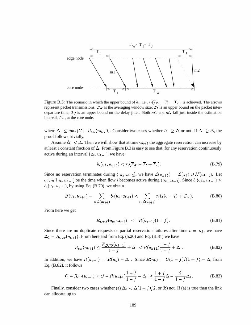
T I T W

T JT I

T JT I --WT

edge node

core node

m2m1

Figure B.3: The scenario in which the upper bound of ��� , i.e., ����� ��� ��� ���� � , is achieved. The arrowsrepresent packet transmissions. � � is the averaging window size; � � is an upper bound on the packet inter-departure time; � � is an upper bound on the delay jitter. Both � and ��� fall just inside the estimationinterval, � � , at the core node.

where � =� � ��� � � � � � � � ��� � � � � � . Consider two cases whether � =

� � or not. If � =� � , the

proof follows trivially.Assume � =

�� . Then we will show that at time � � � � the aggregate reservation can increase by

at least a constant fraction of � . From Figure B.3 is easy to see that, for any reservation continuouslyactive during an interval ��� �

� � � � = � , we have

�

��� �

� � � � = ���

�� � � �� � �� � � (B.79)

Since no reservation terminates during ��� �� � � � = � , we have

� ��� � � = � � � ��� � ��� ��� � � = � . Let���

� ��� �

� � � � = � be the time when flow � becomes active during ��� �� � � � = � . Since

�

� � �

� � � � = � ��

��� �

� � � � = � , by using Eq. (B.79), we obtain

� ��� �� � � � = � �

��� � � � � � �

�

��� �

� � � � = ��

��� � � � � � ��

�� � � �� � � � � (B.80)

From here we get

� ����� ��� �� � � � = �

�� ��� � � = � ��� � � (B.81)

Since there are no duplicate requests or partial reservation failures after time � � � � , we have� = �

����� ��� � � = � . From here and from Eq. (5.20) and Eq. (B.81) we have

� � � � ��� � � = � �� ����� ��� � � = ���� � � =

�� ��� � � = � ��

��� � � = � (B.82)

In addition, we have� ��� � � = �,� � ��� � � � � = . Since

� ��� � � � ��� � � � � � � � � , fromEq. (B.82), it follows

� � � � � � ��� � � = � � � � � ��� � � = � � ��� � � =

� �� ��� � � �

��� � = � (B.83)

Finally, consider two cases whether (a) � =

�� � �� � ��� , or (b) not. If (a) is true then the link

can allocate up to

189

� = � � � � � � � ��� � � = ����� = � � ��� � � �

��� � = � � ��� � � � � = � �

� � � �

(B.84)

capacity during the time interval ��� �� � � � � � . In case (b) we have trivially � =

� � � � � ��� . Thusin both cases we can allocate at least � � � � ��� new capacity during ��� �

� � � � � � .

190