State of the Art of Compactness and Circularity … · International Mathematical Forum, 4, 2009, no. 27, 1305 - 1335 State of the Art of Compactness and Circularity Measures1 Raul

International Mathematical Forum, 4, 2009, no. 27, 1305 - 1335

State of the Art of

Compactness and Circularity Measures1

Raul S. Montero

Departamento de Ciencias de la ComputacionUniversidad Nacional Autnoma de Mexico

Instituto de Investigaciones en Matematicas Aplicadas y en SistemasMexico, Apdo. 20-726, Mexico, D. F., 01000, Mexico

[email protected]

Ernesto Bribiesca

Departamento de Ciencias de la ComputacionUniversidad Nacional Autonoma de Mexico

Instituto de Investigaciones en Matematicas Aplicadas y en SistemasMexico, Apdo. 20-726, Mexico, D. F., 01000, Mexico

[email protected]

Abstract

Compactness is an intrinsic property of objects. This feature is oftenassociated with the old and classical ratio perimeter2/area. This ra-tio is used in many scientific fields as shape descriptor in shape analysistasks. However, when we use this ratio for measuring shape compactnessin the digital domain some problems arise. Several approaches have beenproposed for measuring shape compactness of discrete regions. This pa-per presents a review of several methods for measuring shape circularityand compactness and surveys some of them when scaling transforma-tion is applied to discrete regions. Also, we present a comparison of thestudied methods using the same set of examples of binary shapes underdifferent conditions: shapes with holes and with noisy perimeters.

Mathematics Subject Classification: 68T45

Keywords: shape circularity, shape compactness, shape analysis, shapedescriptor, compactness measures

1306 R. Santiago and E. Bribiesca

1 Introduction

The representation, analysis, and description of the shapes of objects are im-portant topics in pattern recognition and computer vision. Even though sev-eral approaches for describing the shape of objects have been developed in pastdecades [33, 29, 42], one simple shape descriptor has been widely used in pat-tern recognition tasks: shape compactness. Shape compactness is an intrinsiccharacteristic of the shape of objects. The importance of shape compactnessand its utility as shape descriptor has been demonstrated both computer vi-sion [22, 28, 34, 16] and psychological studies [1, 43]. The shape compactnessis frequently included as shape descriptor in diverse shape analysis process[35, 30, 15, 5] and it has been used as the main property to evaluate morpho-logical change in biological entities [31, 7].

Shape compactness is usually associated with the old ratio:

C = P 2/A (1)

Where C is the value of shape compactness, A is the shape area and P isthe shape perimeter. This way to measure shape compactness is taken fromthe isoperimetric inequality.

P 2 ≥ 4πA (2)

The isoperimetric inequality has been used since Babylonian time and thisinequality establishes the isoperimetric problem: What is the domain of aprescribed perimeter enclosing the largest area?. The expression (1) is calledshape compactness [2, 33, 18, 8, 40, 39, 26], circularity [10, 28, 11, 38], dis-persion [1, 19] or roundness measure [23], and sometimes it is expressed asshape factor [12, 25] or P2A. The Greeks used and studied the isoperimetricinequality and knew that a circle is the geometric shape that, for a prescribedperimeter, encloses the largest area [3]. Therefore, a logical consequence is thatthe circle is the most compact shape in the continuous plane. Furthermore, if(1) is used as compactness measure, then we are comparing an object shapewith a circle that has an equal perimeter. Although the P2A is the mostwidely used compactness measure [13], there are more that 20 proposals toevaluate shape compactness in the Euclidean plane [32, 21]. In the case of thecontinuous space, the concept of shape compactness is commonly associatedwith the volumetric version of the isoperimetric inequality

A3 ≥ 36πV 2 (3)

Where A is the enclosing surface of a 3-Dimensional object and V is itsvolume.

State of the art of compactness and circularity measures 1307

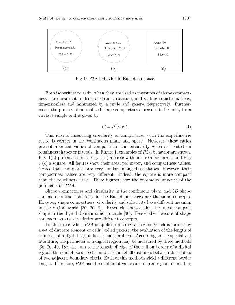
Area=314.15

Perimeter=62.83

P2A=12.56

Area=400

P2A=16

Perimeter=80

Area=319.25

P2A=19.81

Perimeter=79.57

(a) (b) (c)

Fig 1: P2A behavior in Euclidean space

Both isoperimetric radii, when they are used as measures of shape compact-ness , are invariant under translation, rotation, and scaling transformations,dimensionless and minimized by a circle and sphere, respectively. Further-more, the process of normalized shape compactness measure to be unity for acircle is simple and is given by

C = P 2/4πA (4)

This idea of measuring circularity or compactness with the isoperimetricratios is correct in the continuous plane and space. However, these ratiospresent aberrant values of compactness and circularity when are tested onroughness shapes or fractals. In Figure 1, examples of P2A behavior are shown.Fig. 1(a) present a circle, Fig. 1(b) a circle with an irregular border and Fig.1 (c) a square. All figures show their area, perimeter, and compactness values.Notice that shape areas are very similar among these shapes. However, theircompactness values are very different. Indeed, the square is more compactthan the roughness circle. These figures show the enormous influence of theperimeter on P2A.

Shape compactness and circularity in the continuous plane and 3D shapecompactness and sphericity in the Euclidian spaces are the same concepts.However, shape compactness, circularity and sphericity have different meaningin the digital world [36, 20, 8]. Rosenfeld showed that the most compactshape in the digital domain is not a circle [36]. Hence, the measure of shapecompactness and circularity are different concepts.

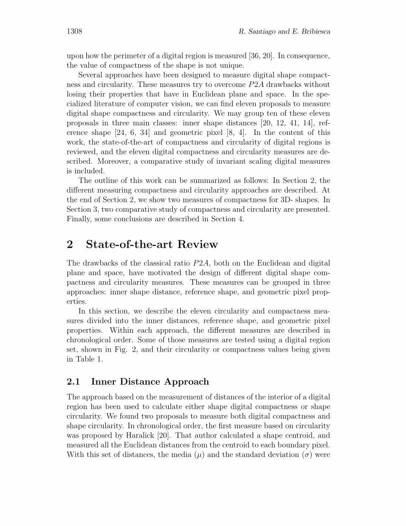
Furthermore, when P2A is applied on a digital region, which is formed bya set of discrete element or cells (called pixels), the evaluation of the length ofa border of a digital region is the main problem. According to the specializedliterature, the perimeter of a digital region may be measured by three methods[36, 20, 40, 18]: the sum of the length of edge of the cell on border of a digitalregion; the sum of border cells; and the sum of all distances between the centersof two adjacent boundary pixels. Each of this methods yield a different borderlength. Therefore, P2A has three different values of a digital region, depending


upon how the perimeter of a digital region is measured [36, 20]. In consequence,the value of compactness of the shape is not unique.

Several approaches have been designed to measure digital shape compact-ness and circularity. These measures try to overcome P2A drawbacks withoutlosing their properties that have in Euclidean plane and space. In the spe-cialized literature of computer vision, we can find eleven proposals to measuredigital shape compactness and circularity. We may group ten of these elevenproposals in three main classes: inner shape distances [20, 12, 41, 14], ref-erence shape [24, 6, 34] and geometric pixel [8, 4]. In the content of thiswork, the state-of-the-art of compactness and circularity of digital regions isreviewed, and the eleven digital compactness and circularity measures are de-scribed. Moreover, a comparative study of invariant scaling digital measuresis included.

The outline of this work can be summarized as follows: In Section 2, thedifferent measuring compactness and circularity approaches are described. Atthe end of Section 2, we show two measures of compactness for 3D- shapes. InSection 3, two comparative study of compactness and circularity are presented.Finally, some conclusions are described in Section 4.

2 State-of-the-art Review

The drawbacks of the classical ratio P2A, both on the Euclidean and digitalplane and space, have motivated the design of different digital shape com-pactness and circularity measures. These measures can be grouped in threeapproaches: inner shape distance, reference shape, and geometric pixel prop-erties.

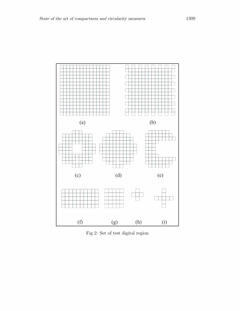
In this section, we describe the eleven circularity and compactness mea-sures divided into the inner distances, reference shape, and geometric pixelproperties. Within each approach, the different measures are described inchronological order. Some of those measures are tested using a digital regionset, shown in Fig. 2, and their circularity or compactness values being givenin Table 1.

2.1 Inner Distance Approach

The approach based on the measurement of distances of the interior of a digitalregion has been used to calculate either shape digital compactness or shapecircularity. We found two proposals to measure both digital compactness andshape circularity. In chronological order, the first measure based on circularitywas proposed by Haralick [20]. That author calculated a shape centroid, andmeasured all the Euclidean distances from the centroid to each boundary pixel.With this set of distances, the media (µ) and the standard deviation (σ) were


(a) (b)

(c) (d) (e)

(f) (g) (h) (i)

Fig 2: Set of test digital region


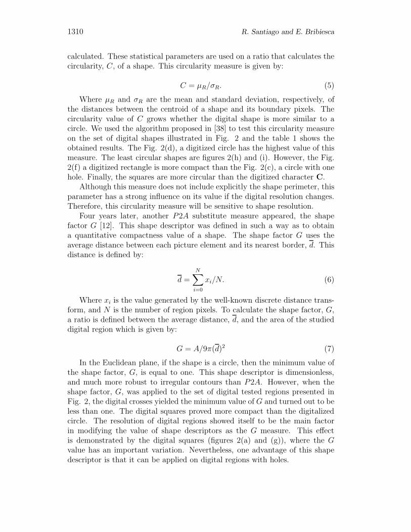
calculated. These statistical parameters are used on a ratio that calculates thecircularity, C, of a shape. This circularity measure is given by:

C = µR/σR. (5)

Where µR and σR are the mean and standard deviation, respectively, ofthe distances between the centroid of a shape and its boundary pixels. Thecircularity value of C grows whether the digital shape is more similar to acircle. We used the algorithm proposed in [38] to test this circularity measureon the set of digital shapes illustrated in Fig. 2 and the table 1 shows theobtained results. The Fig. 2(d), a digitized circle has the highest value of thismeasure. The least circular shapes are figures 2(h) and (i). However, the Fig.2(f) a digitized rectangle is more compact than the Fig. 2(c), a circle with onehole. Finally, the squares are more circular than the digitized character C.

Although this measure does not include explicitly the shape perimeter, thisparameter has a strong influence on its value if the digital resolution changes.Therefore, this circularity measure will be sensitive to shape resolution.

Four years later, another P2A substitute measure appeared, the shapefactor G [12]. This shape descriptor was defined in such a way as to obtaina quantitative compactness value of a shape. The shape factor G uses theaverage distance between each picture element and its nearest border, d. Thisdistance is defined by:

d =

N∑

i=0

xi/N. (6)

Where xi is the value generated by the well-known discrete distance trans-form, and N is the number of region pixels. To calculate the shape factor, G,a ratio is defined between the average distance, d, and the area of the studieddigital region which is given by:

G = A/9π(d)2 (7)

In the Euclidean plane, if the shape is a circle, then the minimum value ofthe shape factor, G, is equal to one. This shape descriptor is dimensionless,and much more robust to irregular contours than P2A. However, when theshape factor, G, was applied to the set of digital tested regions presented inFig. 2, the digital crosses yielded the minimum value of G and turned out to beless than one. The digital squares proved more compact than the digitalizedcircle. The resolution of digital regions showed itself to be the main factorin modifying the value of shape descriptors as the G measure. This effectis demonstrated by the digital squares (figures 2(a) and (g)), where the Gvalue has an important variation. Nevertheless, one advantage of this shapedescriptor is that it can be applied on digital regions with holes.


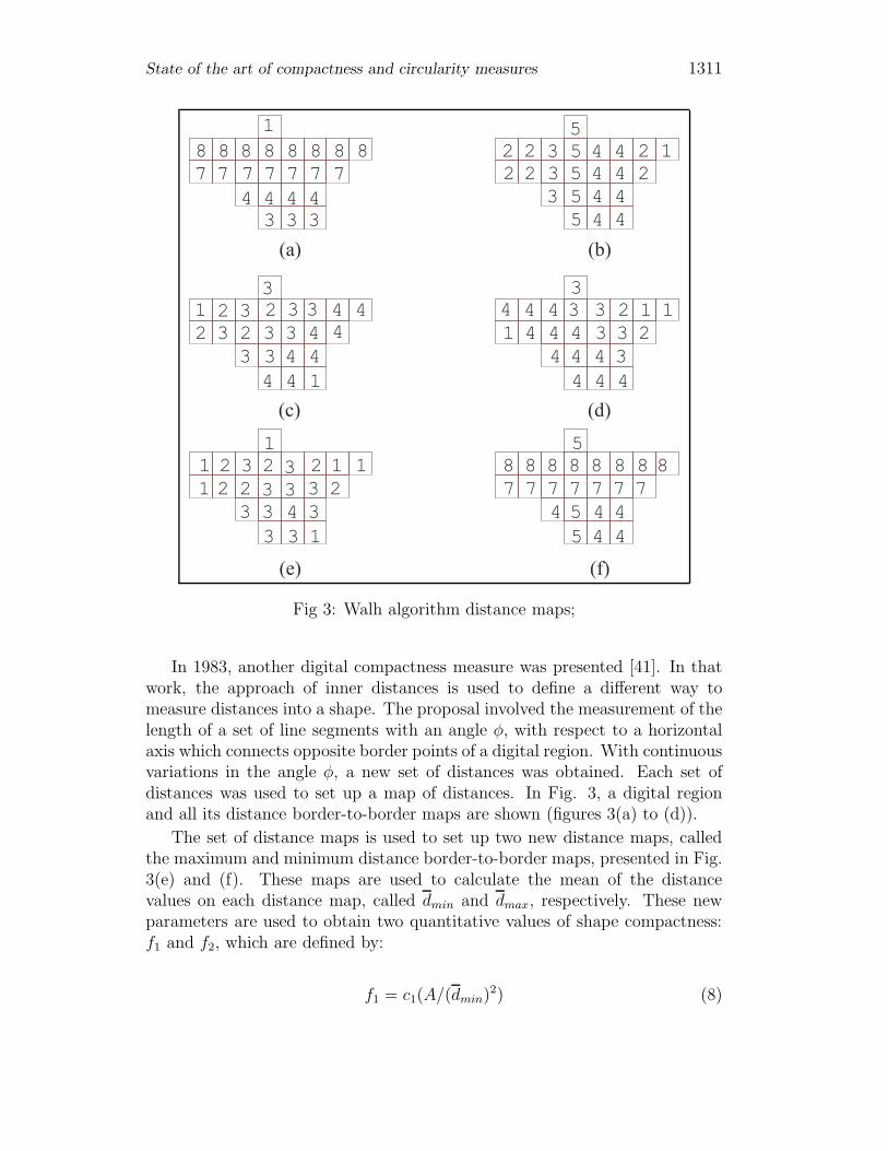
Fig 3: Walh algorithm distance maps;

In 1983, another digital compactness measure was presented [41]. In thatwork, the approach of inner distances is used to define a different way tomeasure distances into a shape. The proposal involved the measurement of thelength of a set of line segments with an angle φ, with respect to a horizontalaxis which connects opposite border points of a digital region. With continuousvariations in the angle φ, a new set of distances was obtained. Each set ofdistances was used to set up a map of distances. In Fig. 3, a digital regionand all its distance border-to-border maps are shown (figures 3(a) to (d)).

The set of distance maps is used to set up two new distance maps, calledthe maximum and minimum distance border-to-border maps, presented in Fig.3(e) and (f). These maps are used to calculate the mean of the distancevalues on each distance map, called dmin and dmax, respectively. These newparameters are used to obtain two quantitative values of shape compactness:f1 and f2, which are defined by:

f1 = c1(A/(dmin)2) (8)


f2 = c2(A/(dmax)2). (9)

Where A is the area of the digital shape, and c1 and c2 are constants equalto 0.6122 and 1.2388, respectively.

Finally, Di Ruperto and Dempster proposed a set of circularity measuresin [14]. They used a mathematical morphology approach to design four ratiosas digital circularity measures. The first circularity measure was denominatedM , and is given by:

M =L∑

i=1

(var{di,j}/max{di,j}). (10)

To calculate this measure, a digital region is eroded with a disk as structureelement, nB, where n is the diameter of disk B. After the last erosion, amaximal region, or a set of maximal regions, is found. Once the maximalregion or regions is found, a set of distances di,j, is calculated from the maximalregion i, in several directions j, 8 or 16 cardinal directions, to the border ofthe digital region. The variance of the distances di,j is var{di,j} and max{di,j}is the maximal distance found for each maximal region.

The second proposed circularity measure was V . This measure is calculatedas the sum of each distance transform values, divided by the cube of themaximum distance transform value, h. This measure is calculated by:

V =∑

p∈X

distX(p)/h3. (11)

The third measure to calculate shape circularity is the T measure, whichuses the area, A, of a digital region. A is divided by the square of the maximumdistance transform value, h, and it is defined by:

T = A/h2. (12)

Finally, the circularity measure, E, is the ratio between the maximum diskthat can be contained in a digital region and the root of its area, A, which isgiven by:

E = n/√

A. (13)

According to Di Ruperto and Dempster, the best results were producedby the measure, M , which is invariant under geometric transformations. Thismeasure evaluates the deformity of a shape by the variance of di,j distances,where the minimum value of M is zero if a shape is a circle. The measure,M , was implemented in this paper using the digital distance transform, andeight cardinal directions were evaluated to obtain the variance value of eachmaximal region. In Table 1, the circularity values of the digital region set


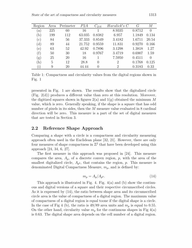
Region Area Perimeter P2A CDN Haralick′s C G M(a) 225 60 16 1 8.9335 0.8712 0(b) 199 112 63.035 0.8382 6.957 1.1849 0.134(c) 84 56 37.333 0.8549 3.4182 1.6711 20.54(d) 89 44 21.752 0.9559 11.831 0.9270 0.166(e) 63 52 42.92 0.7896 3.1298 1.3818 1.27(f) 50 30 18 0.9767 3.4719 0.6907 1.59(g) 25 20 16 1 7.5950 0.4511 0(h) 5 12 28.8 0 2 0.1768 0.125(i) 9 20 44.44 0 2 0.3183 0.33

Table 1: Compactness and circularity values from the digital regions shown inFig. 1

presented in Fig. 1 are shown. The results show that the digitalized circle(Fig. 2(d)) produces a different value than zero at this resolution. Moreover,the digitized squares shown in figures 2(a) and 1(g) obtained the minimum Mvalue, which is zero. Generally speaking, if the shape is a square that has oddnumber of pixels in its sides, then the M measure value evaluated in 8 cardinaldirection will be zero. This measure is a part of the set of digital measuresthat are tested in Section 3.

2.2 Reference Shape Approach

Comparing a shape with a circle is a compactness and circularity measuringapproach often used in the Euclidean plane [32, 21]. However, there are onlyfour measures of shape compactness in Z

2 that have been developed using thisapproach [24, 34, 6, 27].

The first measure in this approach was proposed in [24]. This measurecompares the area, Ap, of a discrete convex region, p, with the area of thesmallest digitalized circle, Ap0, that contains the region, p. This measure isdenominated Digital Compactness Measure, mp, and is defined by:

mp = Ap/Ap0. (14)

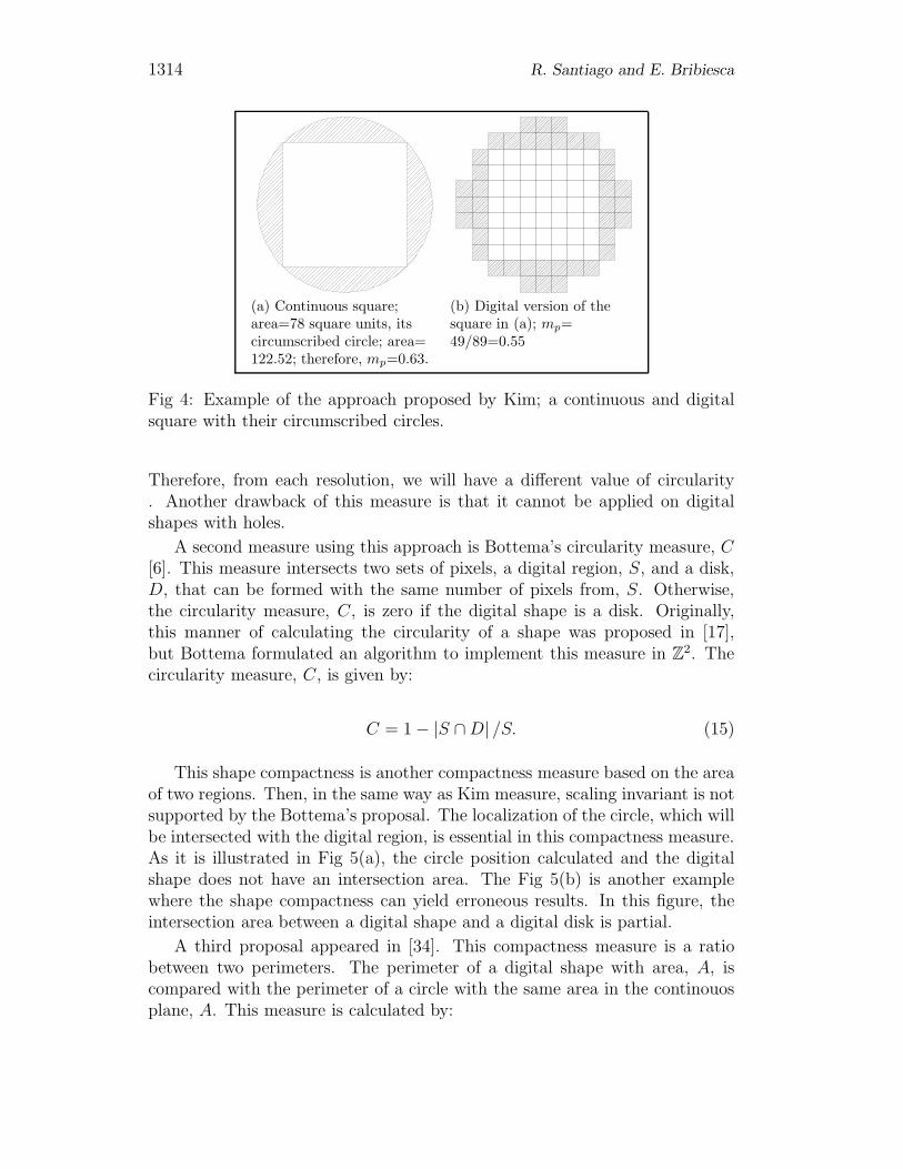
This approach is illustrated in Fig. 4. Fig. 4(a) and (b) show the continu-ous and digital versions of a square and their respective circumscribed circles.As it is expressed by (14), the ratio between shape area and its circumscribedcircle area is the value of compactness of a digital region. The maximum valueof compactness of a digital region is equal toone if the digital shape is a circle.In the case of Fig 4 (b), the ratio is 49/89 area units and mp is equal to 0.55.On the other hand, circularity value mp for the continuous shapes in Fig 4(a)is 0.63. The digital shape area depends on the cell number of a digital region.


(a) Continuous square;area=78 square units, itscircumscribed circle; area=122.52; therefore, mp=0.63.

(b) Digital version of thesquare in (a); mp=49/89=0.55

Fig 4: Example of the approach proposed by Kim; a continuous and digitalsquare with their circumscribed circles.

Therefore, from each resolution, we will have a different value of circularity. Another drawback of this measure is that it cannot be applied on digitalshapes with holes.

A second measure using this approach is Bottema’s circularity measure, C[6]. This measure intersects two sets of pixels, a digital region, S, and a disk,D, that can be formed with the same number of pixels from, S. Otherwise,the circularity measure, C, is zero if the digital shape is a disk. Originally,this manner of calculating the circularity of a shape was proposed in [17],but Bottema formulated an algorithm to implement this measure in Z

2. Thecircularity measure, C, is given by:

C = 1 − |S ∩ D| /S. (15)

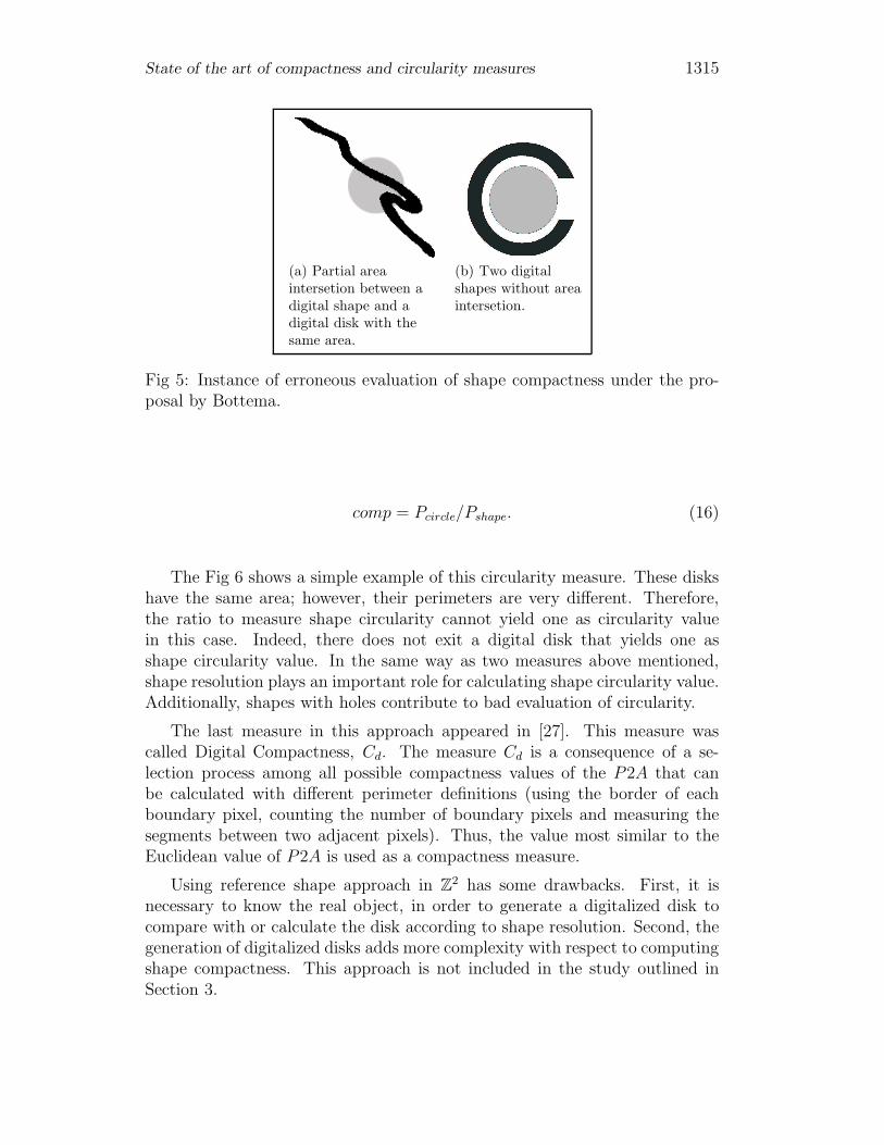
This shape compactness is another compactness measure based on the areaof two regions. Then, in the same way as Kim measure, scaling invariant is notsupported by the Bottema’s proposal. The localization of the circle, which willbe intersected with the digital region, is essential in this compactness measure.As it is illustrated in Fig 5(a), the circle position calculated and the digitalshape does not have an intersection area. The Fig 5(b) is another examplewhere the shape compactness can yield erroneous results. In this figure, theintersection area between a digital shape and a digital disk is partial.

A third proposal appeared in [34]. This compactness measure is a ratiobetween two perimeters. The perimeter of a digital shape with area, A, iscompared with the perimeter of a circle with the same area in the continouosplane, A. This measure is calculated by:


(a) Partial areaintersetion between adigital shape and adigital disk with thesame area.

(b) Two digitalshapes without areaintersetion.

Fig 5: Instance of erroneous evaluation of shape compactness under the pro-posal by Bottema.

comp = Pcircle/Pshape. (16)

The Fig 6 shows a simple example of this circularity measure. These diskshave the same area; however, their perimeters are very different. Therefore,the ratio to measure shape circularity cannot yield one as circularity valuein this case. Indeed, there does not exit a digital disk that yields one asshape circularity value. In the same way as two measures above mentioned,shape resolution plays an important role for calculating shape circularity value.Additionally, shapes with holes contribute to bad evaluation of circularity.

The last measure in this approach appeared in [27]. This measure wascalled Digital Compactness, Cd. The measure Cd is a consequence of a se-lection process among all possible compactness values of the P2A that canbe calculated with different perimeter definitions (using the border of eachboundary pixel, counting the number of boundary pixels and measuring thesegments between two adjacent pixels). Thus, the value most similar to theEuclidean value of P2A is used as a compactness measure.

Using reference shape approach in Z2 has some drawbacks. First, it is

necessary to know the real object, in order to generate a digitalized disk tocompare with or calculate the disk according to shape resolution. Second, thegeneration of digitalized disks adds more complexity with respect to computingshape compactness. This approach is not included in the study outlined inSection 3.


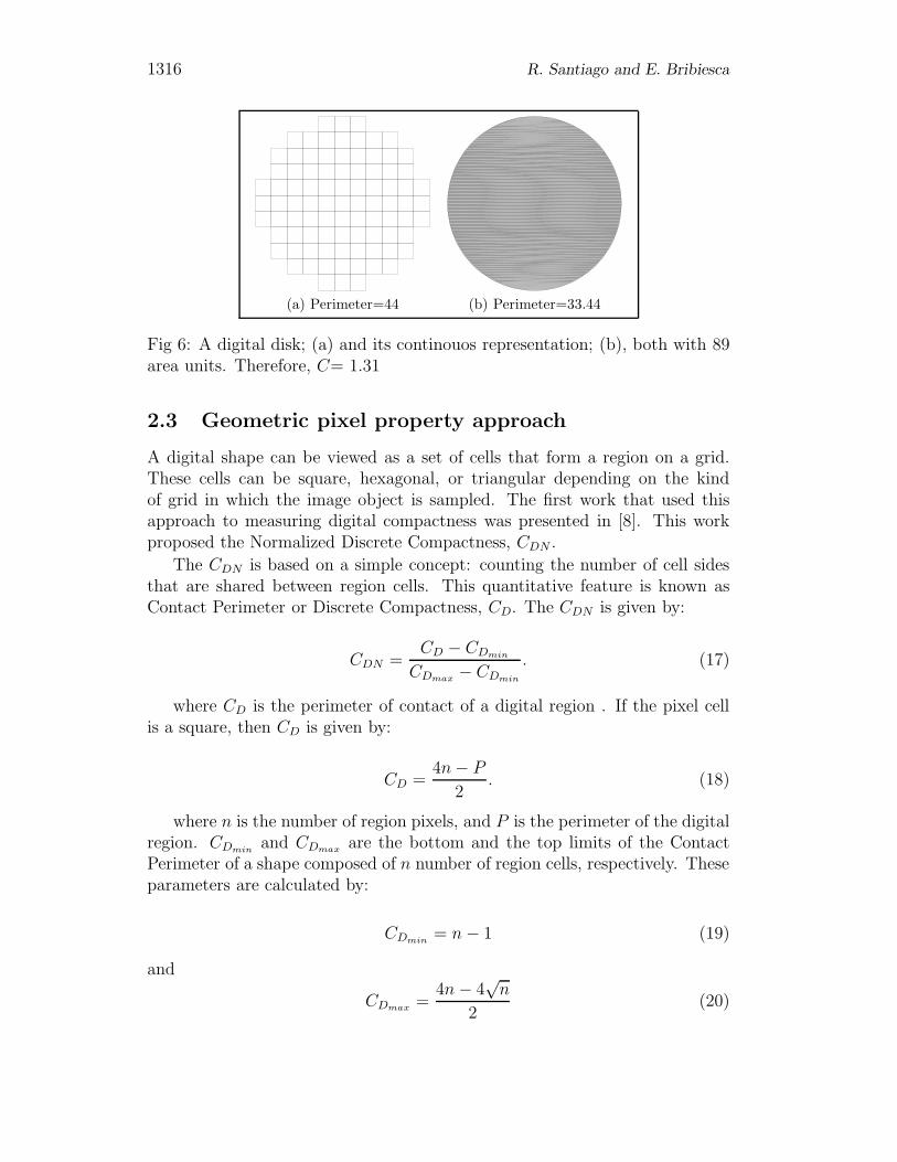
(a) Perimeter=44 (b) Perimeter=33.44

Fig 6: A digital disk; (a) and its continouos representation; (b), both with 89area units. Therefore, C= 1.31

2.3 Geometric pixel property approach

A digital shape can be viewed as a set of cells that form a region on a grid.These cells can be square, hexagonal, or triangular depending on the kindof grid in which the image object is sampled. The first work that used thisapproach to measuring digital compactness was presented in [8]. This workproposed the Normalized Discrete Compactness, CDN .

The CDN is based on a simple concept: counting the number of cell sidesthat are shared between region cells. This quantitative feature is known asContact Perimeter or Discrete Compactness, CD. The CDN is given by:

CDN =CD − CDmin

CDmax− CDmin

. (17)

where CD is the perimeter of contact of a digital region . If the pixel cellis a square, then CD is given by:

CD =4n − P

2. (18)

where n is the number of region pixels, and P is the perimeter of the digitalregion. CDmin

and CDmaxare the bottom and the top limits of the Contact

Perimeter of a shape composed of n number of region cells, respectively. Theseparameters are calculated by:

CDmin= n − 1 (19)

and

CDmax=

4n − 4√

n

2(20)


The Normalized Discrete Compactness is the unique measure of the set ofmeasures described in this paper that has been implemented to 3D shapes [9].The 3D version of CDN is called Discrete Compactness and it is given by:

CD =AC − ACmin

ACmax− ACmin

. (21)

where AC is the contact surface area. If the solid is composed of voxels,then AC is given by:

AC =6an − A

2. (22)

where a is the area of a voxel face, and n is the number of volume vox-els. ACmin

and ACmaxare the minimum and maximum contact surface areas,

respectively. They are calculated by:

ACmin= a(n − 1) (23)

and

ACmax= 3(n − ( 3

√n)2) (24)

Table 1 shows the results of the set of digital regions in Fig 2 for CDN

measure, where the rough square is less compact than the circle, the rectangle,or the circle with a hole. Therefore, the CDN is sensitive to rough contours tosmall resolutions. On the other hand, the digital regions of figures 2(h) and 2(i)obtained the minimum value of CDN without being the most disperse digitalshapes.This measure is included into the set of measures tested in Section 3.

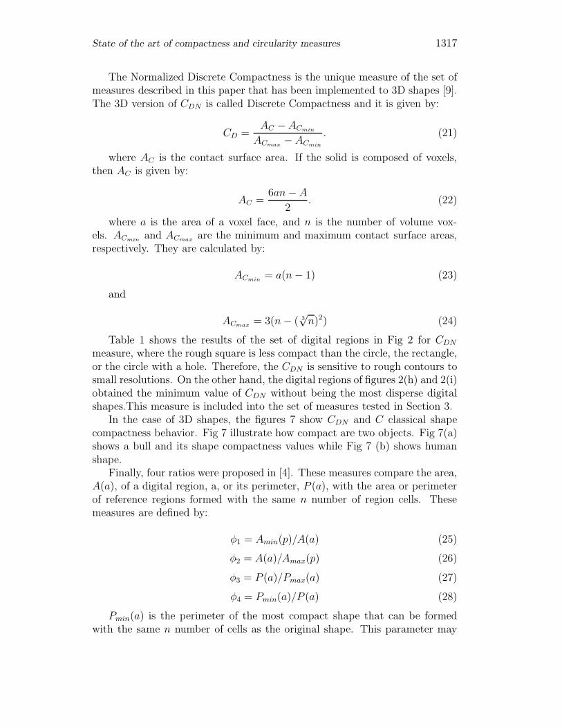
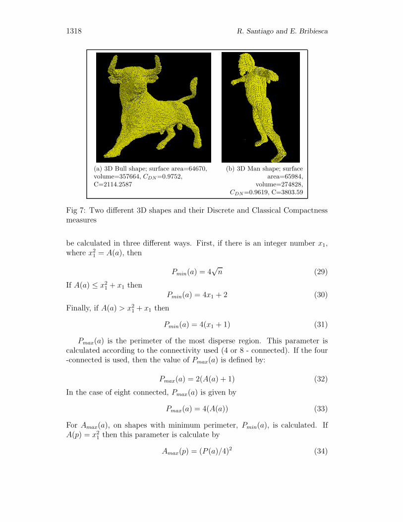
In the case of 3D shapes, the figures 7 show CDN and C classical shapecompactness behavior. Fig 7 illustrate how compact are two objects. Fig 7(a)shows a bull and its shape compactness values while Fig 7 (b) shows humanshape.

Finally, four ratios were proposed in [4]. These measures compare the area,A(a), of a digital region, a, or its perimeter, P (a), with the area or perimeterof reference regions formed with the same n number of region cells. Thesemeasures are defined by:

φ1 = Amin(p)/A(a) (25)

φ2 = A(a)/Amax(p) (26)

φ3 = P (a)/Pmax(a) (27)

φ4 = Pmin(a)/P (a) (28)

Pmin(a) is the perimeter of the most compact shape that can be formedwith the same n number of cells as the original shape. This parameter may


(a) 3D Bull shape; surface area=64670,volume=357664, CDN=0.9752,C=2114.2587

(b) 3D Man shape; surfacearea=65984,

volume=274828,CDN=0.9619, C=3803.59

Fig 7: Two different 3D shapes and their Discrete and Classical Compactnessmeasures

be calculated in three different ways. First, if there is an integer number x1,where x2

1 = A(a), then

Pmin(a) = 4√

n (29)

If A(a) ≤ x21 + x1 then

Pmin(a) = 4x1 + 2 (30)

Finally, if A(a) > x21 + x1 then

Pmin(a) = 4(x1 + 1) (31)

Pmax(a) is the perimeter of the most disperse region. This parameter iscalculated according to the connectivity used (4 or 8 - connected). If the four-connected is used, then the value of Pmax(a) is defined by:

Pmax(a) = 2(A(a) + 1) (32)

In the case of eight connected, Pmax(a) is given by

Pmax(a) = 4(A(a)) (33)

For Amax(a), on shapes with minimum perimeter, Pmin(a), is calculated. IfA(p) = x2

1 then this parameter is calculate by

Amax(p) = (P (a)/4)2 (34)


andAmax(p) = 1/4((P (a)2/4) − 1) (35)

otherwise.The Amin(a) is based on the connectivity used. At four -connectivity, this

parameter is given by:

Amin(p) = (P (a) − 2)/2 (36)

And if the eight -connectivity is used, and the shape contact perimeter,CD, is zero, the minimum area is calculated by:

Amin(p) = P (a)/4 (37)

This set of ratios is very sensitive to the resolution of digital shapes, there-fore, they are not invariant under scaling. The best measure of this set is φ4,however, the authors of this work suggested to use a combination of this mea-sure and the ratio P2A to produce a good measurement of shape compactness.

2.4 Sankar’s compactness measure

There is a measure that cannot be classified using the above-mentioned innershape distances, reference shape and geometric pixel property approaches: thenon-compactness measure designed by Sankar [37]. Sankar saw a digital regionas a lattice, and used his approach to propose a unique manner to measure theperimeter of a digital region without holes. Using this approach, the area of adigital region, S, is defined by:

Ap(S) = 1/2(b + i − 1). (38)

Where b is the number of border points, and i is the number of interiorpoints of S. The perimeter of the digital region is given by:

Pp(S) = 1/2∑

j

p(Xj). (39)

where p(Xj) is the perimeter value in the point Xj ∈ S. p(Xj), which iscalculated by:

p(Xj) =∑

∆∈0,2,4,6

((Xj ∧ Xj,∆)

− (Xj,∆ ∧ (Xj,∆−1 ∨ Xj,∆−2) ∧ (Xj,∆+1 ∨ Xj,∆+2)))

+∑

∆∈1,3,5,7

(2)1

2 ((Xj ∧ Xj,∆)

− (Xj,∆−1 ∧ Xj,∆ ∧ Xj,∆+1)). (40)


Where ∧ and ∨ are the Boolean AND and OR operators, respectively. Thevalue of each Xj,∆ is one if Xj,∆ ∈ S and zero otherwise. Each neighbor of Xj

is determined by the relation of neighborhood described below:

Xj,3 Xj,2 Xj,1

Xj,4 Xj Xj,0

Xj,5 Xj,6 Xj,7

(41)

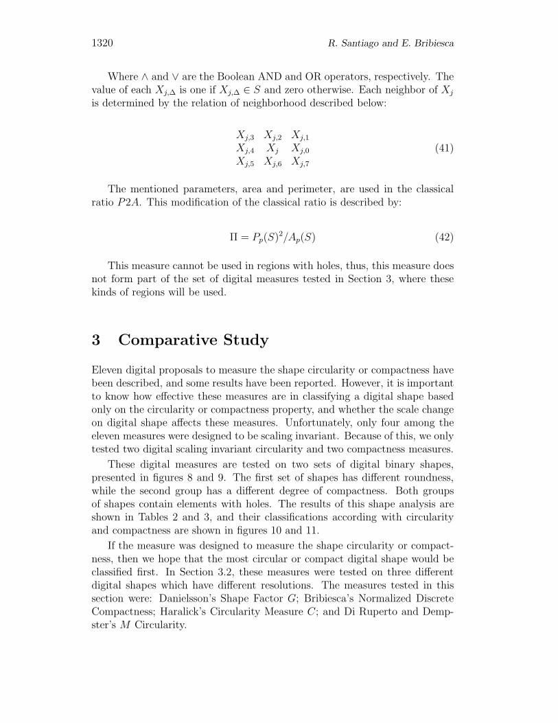
The mentioned parameters, area and perimeter, are used in the classicalratio P2A. This modification of the classical ratio is described by:

Π = Pp(S)2/Ap(S) (42)

This measure cannot be used in regions with holes, thus, this measure doesnot form part of the set of digital measures tested in Section 3, where thesekinds of regions will be used.

3 Comparative Study

Eleven digital proposals to measure the shape circularity or compactness havebeen described, and some results have been reported. However, it is importantto know how effective these measures are in classifying a digital shape basedonly on the circularity or compactness property, and whether the scale changeon digital shape affects these measures. Unfortunately, only four among theeleven measures were designed to be scaling invariant. Because of this, we onlytested two digital scaling invariant circularity and two compactness measures.

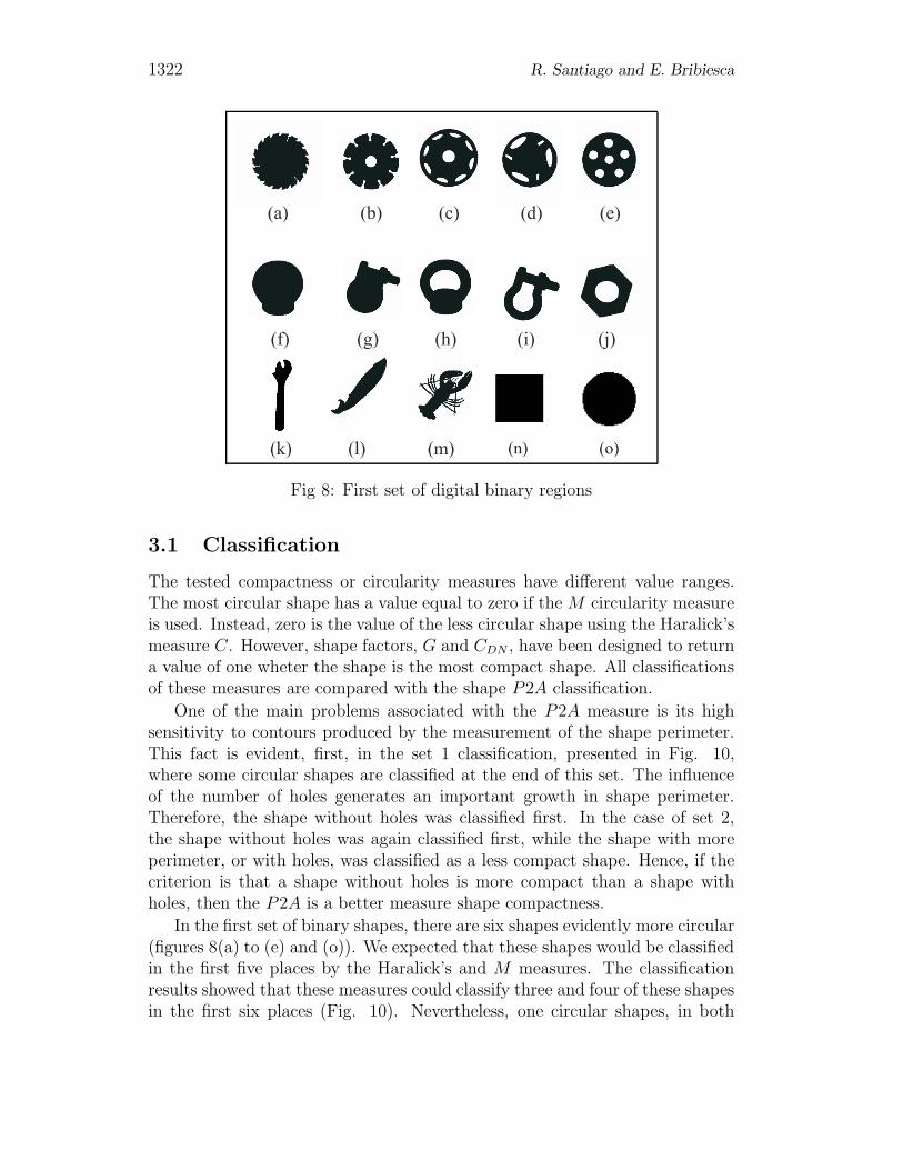
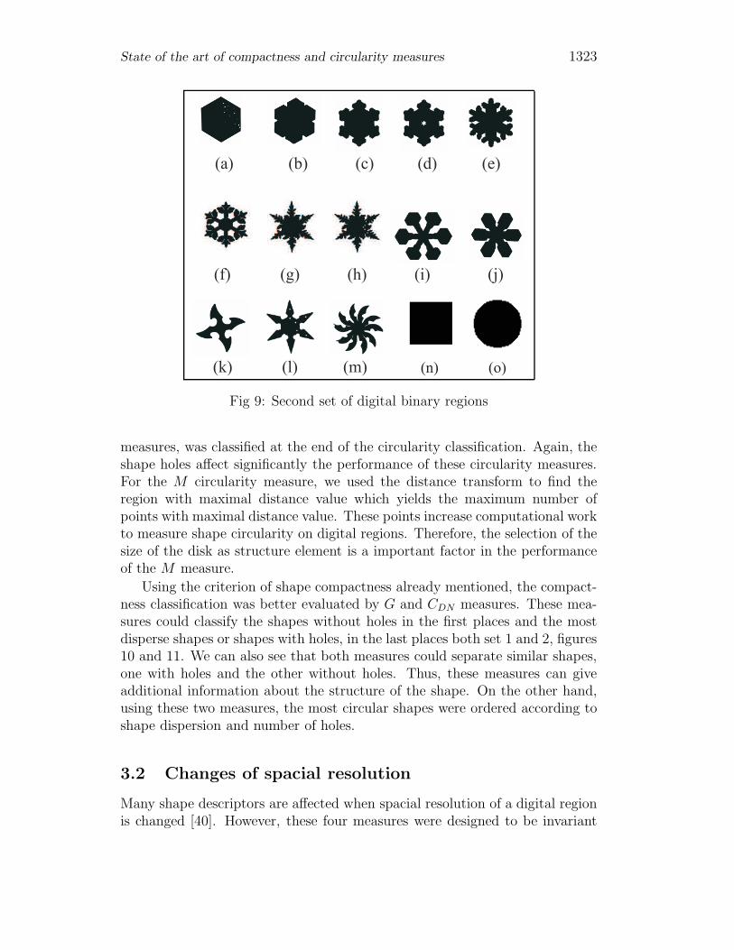
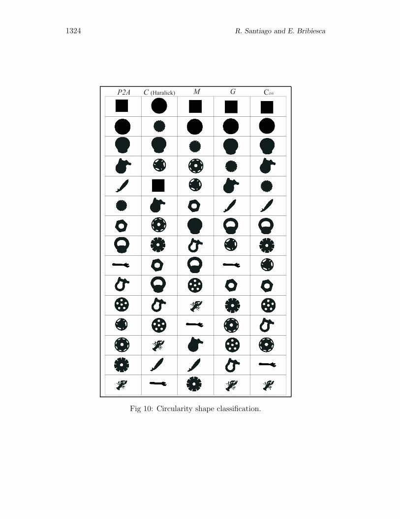
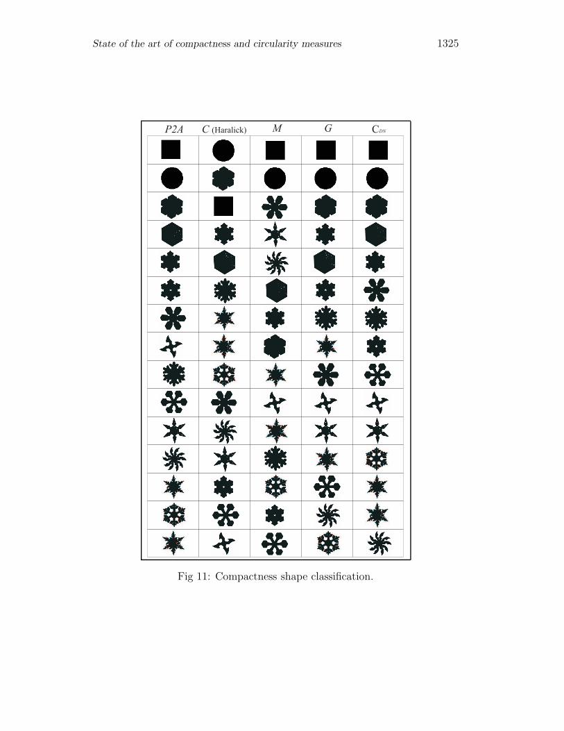
These digital measures are tested on two sets of digital binary shapes,presented in figures 8 and 9. The first set of shapes has different roundness,while the second group has a different degree of compactness. Both groupsof shapes contain elements with holes. The results of this shape analysis areshown in Tables 2 and 3, and their classifications according with circularityand compactness are shown in figures 10 and 11.

If the measure was designed to measure the shape circularity or compact-ness, then we hope that the most circular or compact digital shape would beclassified first. In Section 3.2, these measures were tested on three differentdigital shapes which have different resolutions. The measures tested in thissection were: Danielsson’s Shape Factor G; Bribiesca’s Normalized DiscreteCompactness; Haralick’s Circularity Measure C; and Di Ruperto and Demp-ster’s M Circularity.


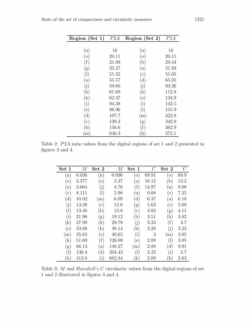
Region (Set 1) P2A Region (Set 2) P2A

(n) 16 (n) 16(o) 20.11 (o) 20.11(f) 21.09 (b) 29.44(g) 33.27 (a) 31.93(l) 51.32 (c) 51.05(a) 55.57 (d) 65.05(j) 59.60 (j) 93.26(h) 61.69 (k) 112.8(k) 62.37 (e) 134.9(i) 94.38 (i) 142.5(e) 98.96 (l) 155.9(d) 107.7 (m) 322.8(c) 139.3 (g) 342.8(b) 156.6 (f) 362.9(m) 640.3 (h) 372.1

Table 2: P2A ratio values from the digital regions of set 1 and 2 presented infigures 3 and 4.

Set 1 M Set 2 M Set 1 C Set 2 C(n) 0.036 (n) 0.036 (o) 69.91 (o) 69.9(o) 2.377 (o) 2.37 (a) 16.12 (b) 13.2(a) 3.064 (j) 4.76 (f) 14.97 (n) 9.08(c) 8.111 (l) 5.98 (n) 9.08 (c) 7.25(d) 10.02 (m) 6.09 (d) 6.37 (a) 6.18(j) 13.38 (c) 12.6 (g) 5.63 (e) 5.68(f) 13.48 (b) 13.8 (c) 3.92 (g) 4.11(i) 21.96 (g) 19.12 (b) 3.51 (h) 3.82(h) 27.99 (k) 29.78 (j) 3.33 (f) 3.7(e) 33.88 (h) 38.14 (h) 3.29 (j) 3.22

(m) 35.62 (e) 40.65 (i) 3 (m) 3.05(k) 51.69 (f) 126.09 (e) 2.89 (l) 3.05(g) 66.14 (a) 148.27 (m) 2.88 (d) 9.91(l) 130.4 (d) 204.42 (l) 2.32 (i) 2.7(b) 413.8 (i) 602.84 (k) 2.09 (k) 2.63

Table 3: M and Haralick′s C circularity values from the digital regions of set1 and 2 illustrated in figures 3 and 4.


(n) (o)

Fig 8: First set of digital binary regions

3.1 Classification

The tested compactness or circularity measures have different value ranges.The most circular shape has a value equal to zero if the M circularity measureis used. Instead, zero is the value of the less circular shape using the Haralick’smeasure C. However, shape factors, G and CDN , have been designed to returna value of one wheter the shape is the most compact shape. All classificationsof these measures are compared with the shape P2A classification.

One of the main problems associated with the P2A measure is its highsensitivity to contours produced by the measurement of the shape perimeter.This fact is evident, first, in the set 1 classification, presented in Fig. 10,where some circular shapes are classified at the end of this set. The influenceof the number of holes generates an important growth in shape perimeter.Therefore, the shape without holes was classified first. In the case of set 2,the shape without holes was again classified first, while the shape with moreperimeter, or with holes, was classified as a less compact shape. Hence, if thecriterion is that a shape without holes is more compact than a shape withholes, then the P2A is a better measure shape compactness.

In the first set of binary shapes, there are six shapes evidently more circular(figures 8(a) to (e) and (o)). We expected that these shapes would be classifiedin the first five places by the Haralick’s and M measures. The classificationresults showed that these measures could classify three and four of these shapesin the first six places (Fig. 10). Nevertheless, one circular shapes, in both


(n) (o)

Fig 9: Second set of digital binary regions

measures, was classified at the end of the circularity classification. Again, theshape holes affect significantly the performance of these circularity measures.For the M circularity measure, we used the distance transform to find theregion with maximal distance value which yields the maximum number ofpoints with maximal distance value. These points increase computational workto measure shape circularity on digital regions. Therefore, the selection of thesize of the disk as structure element is a important factor in the performanceof the M measure.

Using the criterion of shape compactness already mentioned, the compact-ness classification was better evaluated by G and CDN measures. These mea-sures could classify the shapes without holes in the first places and the mostdisperse shapes or shapes with holes, in the last places both set 1 and 2, figures10 and 11. We can also see that both measures could separate similar shapes,one with holes and the other without holes. Thus, these measures can giveadditional information about the structure of the shape. On the other hand,using these two measures, the most circular shapes were ordered according toshape dispersion and number of holes.

3.2 Changes of spacial resolution

Many shape descriptors are affected when spacial resolution of a digital regionis changed [40]. However, these four measures were designed to be invariant


P2A C (Haralick) M G CDN

Fig 10: Circularity shape classification.


P2A C (Haralick) M G CDN

Fig 11: Compactness shape classification.


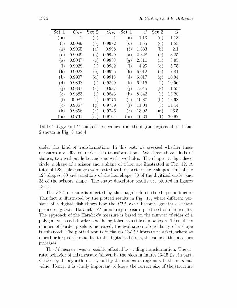
Set 1 CDN Set 2 CDN Set 1 G Set 2 G( n) 1 (n) 1 (n) 1.13 (n) 1.13(f) 0.9989 (b) 0.9982 (o) 1.55 (o) 1.55(g) 0.9965 (a) 0.998 (f) 1.833 (b) 2.1(o) 0.9949 (o) 0.9949 (a) 2.328 (c) 3.25(a) 0.9947 (c) 0.9933 (g) 2.511 (a) 3.85(l) 0.9928 (j) 0.9932 (l) 4.25 (d) 5.75(h) 0.9922 (e) 0.9926 (h) 6.012 (e) 7.81(b) 0.9907 (d) 0.9913 (d) 6.017 (g) 10.04(d) 0.9898 (i) 0.9899 (k) 6.216 (j) 10.06(j) 0.9891 (k) 0.987 (j) 7.046 (k) 11.55(e) 0.9883 (l) 0.9843 (b) 8.342 (l) 12.28(i) 0.987 (f) 0.9776 (c) 10.87 (h) 12.68(c) 0.9867 (g) 0.9759 (i) 11.04 (i) 14.44(k) 0.9856 (h) 0.9746 (e) 13.92 (m) 26.5(m) 0.9731 (m) 0.9701 (m) 16.36 (f) 30.97

Table 4: CDN and G compactness values from the digital regions of set 1 and2 shown in Fig. 3 and 4

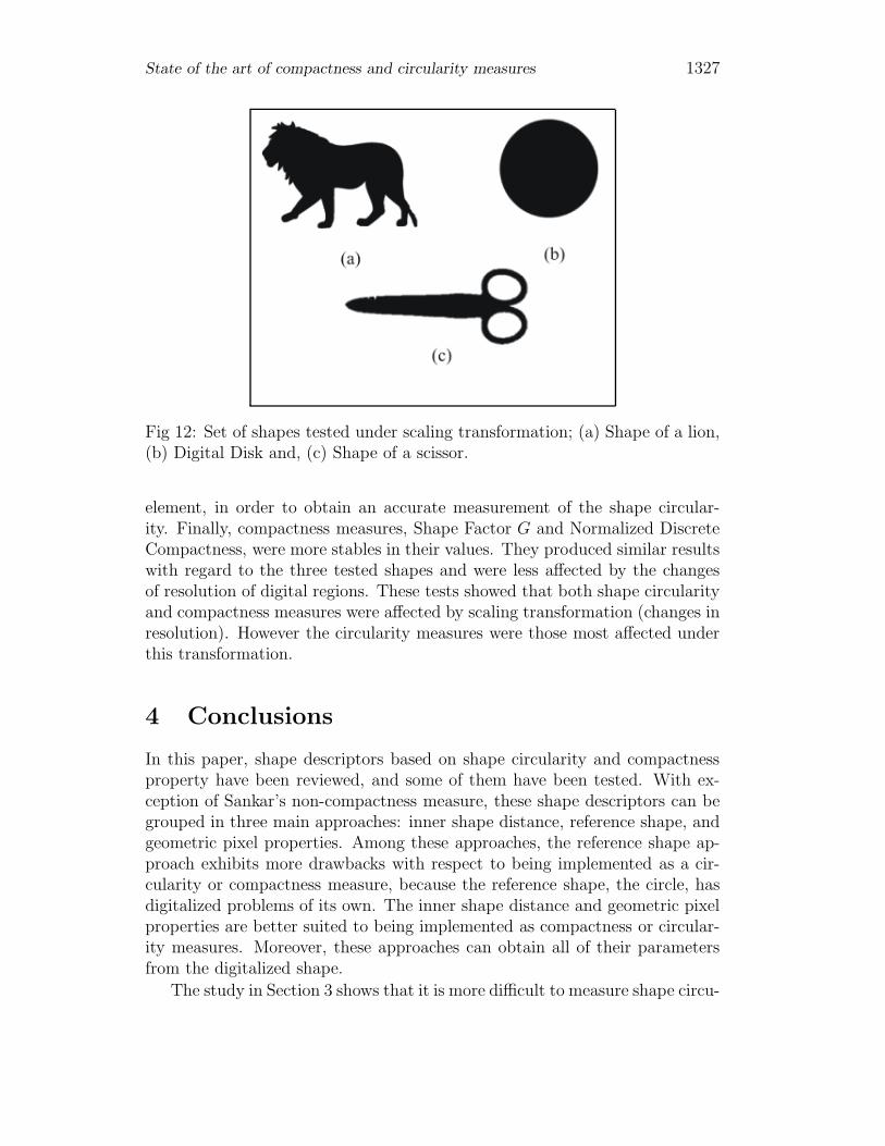
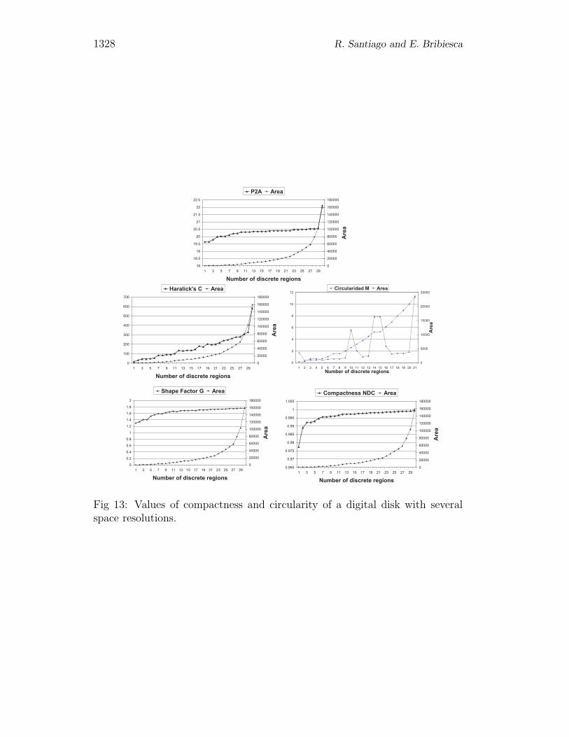
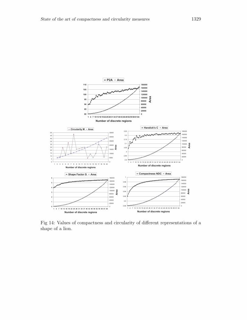
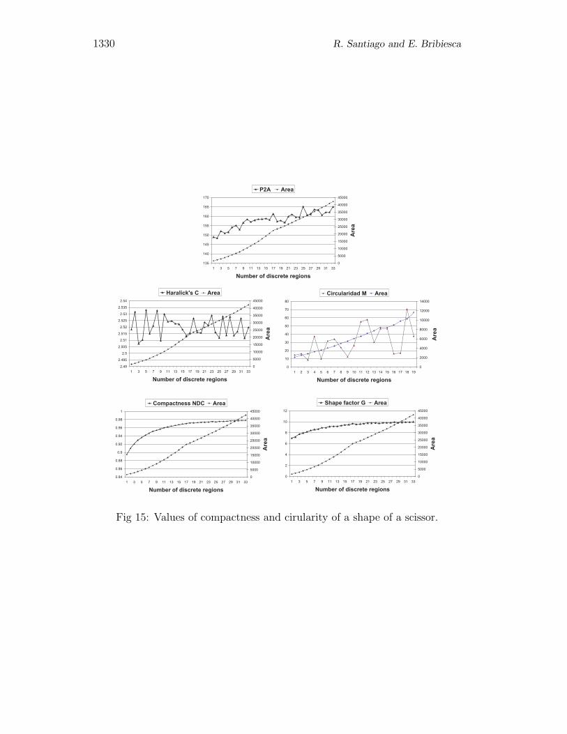
under this kind of transformation. In this test, we assessed whether thesemeasures are affected under this transformation. We chose three kinds ofshapes, two without holes and one with two holes. The shapes, a digitalizedcircle, a shape of a scissor and a shape of a lion are illustrated in Fig. 12. Atotal of 123 scale changes were tested with respect to these shapes. Out of the123 shapes, 60 are variations of the lion shape, 30 of the digitized circle, and33 of the scissors shape. The shape descriptor results are plotted in figures13-15.

The P2A measure is affected by the magnitude of the shape perimeter.This fact is illustrated by the plotted results in Fig. 13, where different ver-sions of a digital disk shows how the P2A value becomes greater as shapeperimeter grows. Haralick’s C circularity measure produced similar results.The approach of the Haralick’s measure is based on the number of sides of apolygon, with each border pixel being taken as a side of a polygon. Thus, if thenumber of border pixels is increased, the evaluation of circularity of a shapeis enhanced. The plotted results in figures 13-15 illustrate this fact, where asmore border pixels are added to the digitalized circle, the value of this measureincreases.

The M measure was especially affected by scaling transformation. The er-ratic behavior of this measure (shown by the plots in figures 13-15 )is , in part,yielded by the algorithm used, and by the number of regions with the maximalvalue. Hence, it is vitally important to know the correct size of the structure


Fig 12: Set of shapes tested under scaling transformation; (a) Shape of a lion,(b) Digital Disk and, (c) Shape of a scissor.

element, in order to obtain an accurate measurement of the shape circular-ity. Finally, compactness measures, Shape Factor G and Normalized DiscreteCompactness, were more stables in their values. They produced similar resultswith regard to the three tested shapes and were less affected by the changesof resolution of digital regions. These tests showed that both shape circularityand compactness measures were affected by scaling transformation (changes inresolution). However the circularity measures were those most affected underthis transformation.

4 Conclusions

In this paper, shape descriptors based on shape circularity and compactnessproperty have been reviewed, and some of them have been tested. With ex-ception of Sankar’s non-compactness measure, these shape descriptors can begrouped in three main approaches: inner shape distance, reference shape, andgeometric pixel properties. Among these approaches, the reference shape ap-proach exhibits more drawbacks with respect to being implemented as a cir-cularity or compactness measure, because the reference shape, the circle, hasdigitalized problems of its own. The inner shape distance and geometric pixelproperties are better suited to being implemented as compactness or circular-ity measures. Moreover, these approaches can obtain all of their parametersfrom the digitalized shape.

The study in Section 3 shows that it is more difficult to measure shape circu-


0

100

200

300

400

500

600

700

1 3 5 7 9 11 13 15 17 19 21 23 25 27 29

Number of discrete regions

0

20000

40000

60000

80000

100000

120000

140000

160000

180000

Are

a

Haralick's C Area

18

18.5

19

19.5

20

20.5

21

21.5

22

22.5

1 3 5 7 9 11 13 15 17 19 21 23 25 27 29


0

20000

40000

60000

80000

100000

120000

140000

160000

180000

Are

a

P2A Area

0

0.2

0.4

0.6

0.8

1

1.2

1.4

1.6

1.8

2

1 3 5 7 9 11 13 15 17 19 21 23 25 27 29


0

20000

40000

60000

80000

100000

120000

140000

160000

180000

Are

a

Shape Factor G Area

0.965

0.97

0.975

0.98

0.985

0.99

0.995

1

1.005

1 3 5 7 9 11 13 15 17 19 21 23 25 27 29


0

20000

40000

60000

80000

100000

120000

140000

160000

180000

Are

a

Compactness NDC Area

0

2

4

6

8

10

12

1 2 3 4 5 6 7 8 9 10 11 12 13 14 15 16 17 18 19 20 21


0

5000

10000

15000

20000

25000

Are

a

Circularidad M Area

Fig 13: Values of compactness and circularity of a digital disk with severalspace resolutions.


0.88

0.9

0.92

0.94

0.96

0.98

1

1 4 7 10 13 16 19 22 25 28 31 34 37 40 43 46 49 52 55 58 61 64


0

20000

40000

60000

80000

100000

120000

140000

160000

180000

Are

a


2.9

2.95

3

3.05

3.1

3.15

3.2

3.25

1 4 7 10 13 16 19 22 25 28 31 34 37 40 43 46 49 52 55 58 61 64


0

20000

40000

60000

80000

100000

120000

140000

160000

180000

Are

a

Haralick's C Area

0

1

2

3

4

5

6

1 4 7 10 13 16 19 22 25 28 31 34 37 40 43 46 49 52 55 58 61 64


0

20000

40000

60000

80000

100000

120000

140000

160000

180000

Are

a

Shape Factor G Area

80

85

90

95

100

105

110

1 4 7 10131619222528313437404346495255586164


0

20000

40000

60000

80000

100000

120000

140000

160000

180000

Are

a

P2A Area

0

5

10

15

20

25

30

35

40

45

50

1 2 3 4 5 6 7 8 9 10 11 12 13 14 15 16 17 18 19 20


0

5000

10000

15000

20000

25000

30000

35000

Are

a

Circularity M Area

Fig 14: Values of compactness and circularity of different representations of ashape of a lion.


135

140

145

150

155

160

165

170

1 3 5 7 9 11 13 15 17 19 21 23 25 27 29 31 33


0

5000

10000

15000

20000

25000

30000

35000

40000

45000

Are

a

P2A Area

0.84

0.86

0.88

0.9

0.92

0.94

0.96

0.98

1

1 3 5 7 9 11 13 15 17 19 21 23 25 27 29 31 33


0

5000

10000

15000

20000

25000

30000

35000

40000

45000

Are

a


2.49

2.495

2.5

2.505

2.51

2.515

2.52

2.525

2.53

2.535

2.54

1 3 5 7 9 11 13 15 17 19 21 23 25 27 29 31 33


0

5000

10000

15000

20000

25000

30000

35000

40000

45000

Are

a

Haralick's C Area

0

2

4

6

8

10

12

1 3 5 7 9 11 13 15 17 19 21 23 25 27 29 31 33


0

5000

10000

15000

20000

25000

30000

35000

40000

45000

Are

a

Shape factor G Area

0

10

20

30

40

50

60

70

80

1 2 3 4 5 6 7 8 9 10 11 12 13 14 15 16 17 18 19


0

2000

4000

6000

8000

10000

12000

14000

Are

a

Circularidad M Area

Fig 15: Values of compactness and cirularity of a shape of a scissor.


larity than shape compactness. The two circularity measures exhibited impor-tant variations in their values under changes of resolution, M and Haralick′sC, and had more problems with respect to classification of shapes by theircircularity property. The holes increased the difficulty when using these mea-sures. In contrast, the two compactness measures, Shape Factor G and CDN ,performed better with respect to evaluating the set of digitized shapes basedon compactness characteristic. Furthermore, the compactness measures testedcould tell us more about the structure of a shape, since they are able to yielda different value depending on whether similar shapes have holes or not. Al-though all the shape descriptors were affected by scale changes, the compact-ness measures were less affected in our tests. Finally, if the measure producesimportant variations in its circularity or compactness value, then this wouldhave to be considered a further disadvantage, additional to those already men-tioned for these kind of measures. Therefore, the universe of shapes can bemixed more easily and produce aberrant classifications.

1 This work is a section of the Doctoral Dissertation of RaulSantiago Montero presented to Universidad Nacional Autonoma deMexico, under the direction of Dr. Ernesto Bribiesca.

ACKNOWLEDGEMENTS. This work was, in part, supportedby the CONACyT (PhD. scholarship 191650) and the UNAM. Wewish to express our gratitude to IIMAS-UNAM and we would alsolike to thank Dr. Yann Frauel for his assistance in reviewing thiswork.

References

[1] F. Attneave and M. D. Arnoult. The quantitative study of shapeand pattern perception. Psychological Bulletin, 53(6):452–471,1956.

[2] D. H. Ballard and C. M. Brown. Computer Vision. PrenticeHall, New Jersey, USA, 1982.

[3] Catherine Blandle. Isoperimetric inequalities and applications.Pitman, Boston, 1980.

[4] J. Bogaert, R. Rousseau, P. Van Hecke, and I. Impens. Alter-native area-perimeter ratios for measurement of 2d shape com-pactness of habitats. Applied Mathematics and Computation,111(1):71–85, 2000.


[5] J. Bogaert, L. Zhou, C. J. Tucker, R. B. Myneni, and R. Ceule-mans. Evidence for a persistent and extensive greening trend ineurasia inferred from satellite vegetation index data. Journal

of Geophysical Research, 107(D11):4–1, 4–13, 2002.

[6] M. J. Bottema. Circularity of objects in images. In Interna-

tional Conference on Acoustic, Speech and Signal Processing,

ICASSP 2000, pages 2247–2250, Istanbul,, 2000. IEEE.

[7] U. D. Braumann, J. P. Kuska, J. Einenkel, L. C. Horn, M. Lof-fler, and M. Hockel. Three-dimensional reconstruction andquantification of cervical carcinoma invasion fronts from his-tological serial sections. Medical Imaging, IEEE Transactions

on, 24(10):1286–1307, 2005.

[8] E. Bribiesca. Measuring 2-d shape compactness using the con-tact perimeter. Computer and Mathematics with Applications,33(11):1–9, 1997.

[9] E. Bribiesca. A measure of compactness for 3d shapes. Com-

puter and Mathematics with Applications, 40:1275–1284, 2000.

[10] K. R. Castleman. Digital Image Processing. Prentice Hall,USA, 1995.

[11] L. F. Costa and R. M. Cesar. Shape Analysis and Classifica-

tion: Theory and Practice. CRC Press, Boca Raton, Florida,USA, 2000.

[12] P. E. Danielsson. A new shape factor. Computer Graphics and

Image Processing, 7(2):292–299, 1978.

[13] E. R. Davies. Machine Vision, Theory, Algoritnms, Practical-

ities. Morgan Kauffmann, USA, 2005.

[14] C. Di Ruperto and A. Dempster. Circularity measures basedon mathematical morphology. Electronics Letters, 36(20):1691–1693, 2000.

[15] R. Edler, D. Wertheim, and D. Greenhill. Outcome mea-surement in the correction of mandibular asymmetry. Amer-

ican Journal of Orthodontics and Dentofacial Orthopedics,125(4):435–443, 2004.


[16] J. D. Edwards, K. J. Riley, and J. P. Eakins. A visual com-parison of shape descriptors using multi-dimensional scaling. InNicolai Petkov and M. A. Westenberg, editors, 10th Interna-

tional Conference, CAIP 2003, pages 393–401, 2003.

[17] M. L. Giger, K. Doi, and H. MacMahon. Image feature analysisand computer-aided diagnossis in digital radiography. 3. auto-mated detection of nodules in peripheral lung fields. Medical

Physics, 15(2):158–166, 1988.

[18] R. C. Gonzalez and R. E. Woods. Digital Image Processing.Prentice Hall, Upper Saddle, New Jersey, USA, 2001.

[19] S. B. Gray. Local properties of binary images in two dimensions.IEEE Trans. on Computer, C-20:551–561, 1971.

[20] R. M. Haralick. A measure for circularity of digital figures.IEEE Transactions on Systems, Man and Cybernetics, SMC-4(4):334–336, 1974.

[21] D. L. Horn, C. R. Hampton, and A. J. Vandenberg. Practi-cal application of district compactness. Political Geography,12(2):103–120, 1993.

[22] S. Ishikawa. Geometrical indices characterizing psychologicalgoodness of random shapes. In Proceedings of the 4th Inter-

national Joint Conference on Pattern Recognition, volume 1,pages 414–416, Kyoto, Japan, 1978.

[23] A. K. Jain. Fundamentals of Digital Image Processing. Pren-tice Hall, USA, 1989.

[24] C. E. Kim and T. A. Anderson. Digital disks and a digital com-pactness measure. In Annual ACM Symposium on Theory of

Computing, Proceedings of the sixteenth annual ACM sympo-

sium on Theory of computing, pages 117–124, New York, N.Y., USA, 1984.

[25] P. W. Kitchin. Processing of binary images. In A. Pugh, editor,Robot Vision, pages 21–42. Springer, Germany, 1983.

[26] R. Klette and A. Rosenfeld. Digital Geometry, Geometric

methods for digital pictures analysis. Morgan Kaufmann, USA,2004.


[27] S. C. Lee, Y. Wang, and E. T. Lee. Compactness measure of dig-ital shapes. In IEEE Region 5 Conference, Annual Technical

and Leadership Workshop, pages 103–105, 2004.

[28] M. D. Levine. Vision in Man and Machine. McGraw-Hill,USA, 1985.

[29] S. Loncaric. A survey of shape analysis techniques. Pattern

Recognition, 31(8):983–1001, 1998.

[30] N. MacLeod. Geometric morphometrics and geological shape-classification systems. Earth-Science Reviews, 59:27–47, 2002.

[31] V. Metzler, T. Lehmann, H. Bienert, K. Mottaghy, andK. Spitzer. A novel method for quantifying shape deformationapplied to biocompatibility testing. ASAIO Journal, 45(4):264–271, 1999.

[32] R. G. Niemi, B. Grofman, C. Carlucci, and T. Hofeller. Mea-suring compactness and the role of a compactness standard ina test for partisan and racial gerrymandering. Journal of Pol-

itics, 22(4):1155–1181, 1990.

[33] T. Pavlidis. Algorithms for shape analysis of contours and wave-forms. IEEE Transactions on Pattern Analysis and Machine

Intelligence, PAMI-2(4):301–312, 1980.

[34] M. Peura and J. Iivarinen. Efficiency of simple shape descrip-tors. In C. Arcelli, P. Cordella, and G Sanniti di Baja, editors,Advances in Visual Form Analysis, pages 443–451. World Sci-entific, Singapore, 1997.

[35] R. M. Rangayyan, N. M El-Faramawy, J. E. L. Desuatels, andO. A. Alim. Measures of acutance and shape for classificationof breast tumors. IEEE Trans. on Medical Imaging, 16(6):799–810, 1997.

[36] A. Rosenfeld. Compact figures in digital pictures. IEEE Trans.

Systems, Man and Cybernetics, 4:221–223, 1974.

[37] P. V. Sankar and E. V. Krishnamurthy. On the compactnessof subsets of digital pictures. Computer Graphics and Image

Processing, 8:136–143, 1978.

[38] L. G. Shapiro and G. C. Stockman. Computer Vision. PrenticeHall, Upper Saddle River, New Jersey, USA, 2001.


[39] E. W. Snyder and H. Qi. Machine Vision. Cambridge Univer-sity Press, United Kingdom, 2004.

[40] M. Sonka, V. Hlavac, and R. Boyle. Image Processing: Analysis

and Machine Vision. Brooks Cole, Mexico City, Mexico, 1998.

[41] F. M. Wahl. A new distance mapping and its use for shapemeasurement on binary patterns. Computer Vision, Graphics

and Image Processing, 23:218–226, 1983.

[42] D. Zhang and G. Lu. Review of shape representation and de-scription techniques. Pattern Recognition, 37:1–19, 2004.

[43] L. Zusne. Moments of area and of the perimeter of visual formsas predictors of discrimination performance. Journal of Exper-

imental Psychology, 69(3):213–220, 1965.

Received: May, 2008

Documents

State of the Art of Compactness and Circularity … · International Mathematical Forum, 4, 2009, no. 27, 1305 - 1335 State of the Art of Compactness and Circularity Measures1 Raul