Embed Size (px)
Citation preview
Topology (H) Lecture 10Lecturer: Zuoqin WangTime: April 12, 2021
COMPACTNESS OF PRODUCT SPACE
1. Compactness of finite products
¶ The tube lemma.
Today we study the compactness of products of compact spaces To prove thecompactness of the product of two compact spaces, we need the tube lemma. Youshould be aware of the use of the “local-to-global principal” in the proof.
Lemma 1.1 (The tube lemma). If A ⊂ X, B ⊂ Y are compact, N ⊂ X × Y is open,and A×B ⊂ N , then there exists open sets U in X and V in Y s.t.
A×B ⊂ U × V ⊂ N.
Proof. We first prove a “basic tube lemma”: the tube lemma holds for A = {x0}. Forany (x0, y0) ∈ X × Y, one can find an open set Uy0
x0in X and an open set Vy0 in Y s.t.
(x0, y0) ∈ Uy0x0× Vy0 ⊂ N.
Since B =Sy∈B{y} ⊂
Sy∈Y Vy, we can find y1, · · · , yk ∈ Y s.t.
B ⊂[
1≤i≤kVyi =: V.
Let U =Tki=1 U
yix0, then U is open and x0 ∈ U ⊂ Uyi
x0, ∀1 ≤ i ≤ k. Moreover,
N ⊃[y
(Uyx0× Vy) ⊃
[1≤i≤k
(Uyix0× Vyi) ⊃
[1≤i≤k
(U × Vyi) = U ×[
1≤i≤kVyi = U × V.
Now we prove the tube lemma. For each x0 ∈ A, by the basic tube lemma, thereexists open sets Ux0 and Vx0 s.t.
{x0} ×B ⊂ Ux0 × Vx0 ⊂ N.
Since A is compact, there exist x1, · · · , xm ∈ A s.t.
A ⊂ Ux1 ∪ · · · ∪ Uxm =: U.
Let V = ∩mi=1Vxi , then B ⊂ V and V is open. So
A×B ⊂ U × V ⊂[
1≤i≤m(Uxi × Vxi) ⊂ N. �
Remark 1.2. It is easy to construct a counterexample if A or B is non-compact: InR× R, we have {0} × R ⊂ N = {(x, y) | |xy| < 1}. But there is no open set U ⊃ {0}such that U × R ⊂ N .
1

2 COMPACTNESS OF PRODUCT SPACE
¶ Compactness of a finite product.
As a consequence, we prove
Proposition 1.3. If A ⊂ X,B ⊂ Y are compact, so is A×B.
Proof. Let W be any open covering of A × B. For any x0 ∈ A, since {x0} × B is
compact1, one can find W(0)1 , · · · ,W (0)
k ∈ W s.t.
{x0} ×B ⊂ W(0)1 ∪ · · · ∪W
(0)k .
By the basic tube lemma, there exists an open set Ux0 in X containing x0 s.t.
Ux0 ×B ⊂ W(0)1 ∪ · · · ∪W
(0)k .
Now {Ux0 | x0 ∈ A} is an open covering of A. By compactness, there existx1, · · · , xm s.t. A ⊂ Ux1 ∪ · · · ∪ Uxm . According to the argument above, for 1 ≤ i ≤ m,
we already find W(i)1 , · · · ,W (i)
k(i) ∈ W s.t.
Uxi ×B ⊂ W(i)1 ∪ · · · ∪W
(i)k(i).
It follows that
A×B ⊂ (Ux1 ∪ · · · ∪ Uxm)×B ⊂[
1≤i≤m,1≤j≤k(i)W
(i)j ,
i.e. {W (i)j | 1 ≤ i ≤ m, 1 ≤ j ≤ k(i)} is a finite sub-covering of W . �
By induction one immediately gets
Corollary 1.4. If X1, · · · , Xk are compact, so is X1 × · · · ×Xk.
¶ Tychonoff Theorem.
Now we state one of the most surprising, important and useful theorems in generaltopology: Tychonoff theorem. It was first proved in a special case by A.N. Tychnoff(also translated as Tikhonov) in 1930, who stated the general version in 19352:
Theorem 1.5 (Tychonoff Theorem).If Xα is compact for each α, then the product (
QαXα,Tproduct) is compact.
At first glance, it seems that the theorem is unlikely to be true. Compactness is aclose relative to “finiteness”. How could an infinite or even an uncountable product be
1You can prove this directly by definition, or by realizing {x0} × B as the image of the compactset B under a continuous map, namely, the embedding map from Y to X × Y mapping y to (x0, y).
2In fact, Tychonoff defined the product topology in his 1935 paper for the first time.
COMPACTNESS OF PRODUCT SPACE 3
compact?! However: let’s look at a couple examples from which we can see compactnessfrom an infinite product. Recall that
XN =Yn∈N
X = {(a1, a2, · · · ) | ai ∈ N}.
As we have seen, the product topology on XN can be identified with the pointwiseconvergence topology on M(N, X). We may look at two examples:
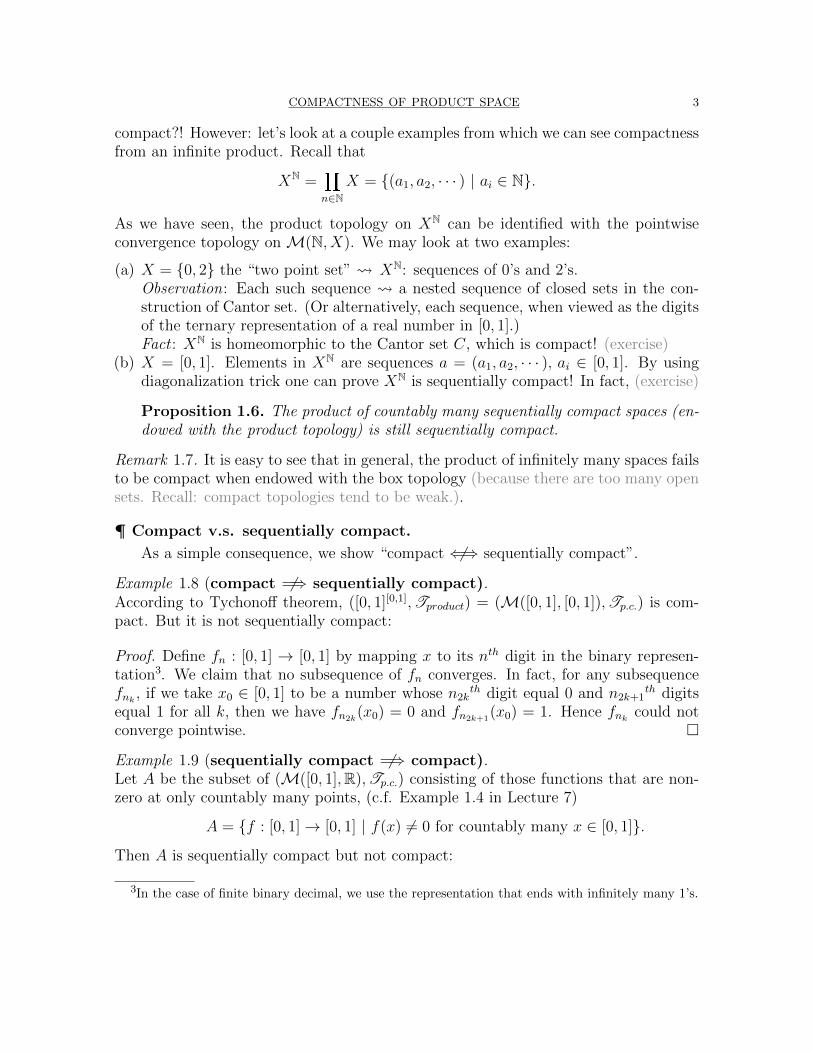
(a) X = {0, 2} the “two point set” XN: sequences of 0’s and 2’s.Observation: Each such sequence a nested sequence of closed sets in the con-struction of Cantor set. (Or alternatively, each sequence, when viewed as the digitsof the ternary representation of a real number in [0, 1].)Fact : XN is homeomorphic to the Cantor set C, which is compact! (exercise)
(b) X = [0, 1]. Elements in XN are sequences a = (a1, a2, · · · ), ai ∈ [0, 1]. By usingdiagonalization trick one can prove XN is sequentially compact! In fact, (exercise)
Proposition 1.6. The product of countably many sequentially compact spaces (en-dowed with the product topology) is still sequentially compact.
Remark 1.7. It is easy to see that in general, the product of infinitely many spaces failsto be compact when endowed with the box topology (because there are too many opensets. Recall: compact topologies tend to be weak.).
¶ Compact v.s. sequentially compact.
As a simple consequence, we show “compact 6⇐⇒ sequentially compact”.
Example 1.8 (compact 6=⇒ sequentially compact).According to Tychonoff theorem, ([0, 1][0,1],Tproduct) = (M([0, 1], [0, 1]),Tp.c.) is com-pact. But it is not sequentially compact:
Proof. Define fn : [0, 1] → [0, 1] by mapping x to its nth digit in the binary represen-tation3. We claim that no subsequence of fn converges. In fact, for any subsequencefnk , if we take x0 ∈ [0, 1] to be a number whose n2k
th digit equal 0 and n2k+1th digits
equal 1 for all k, then we have fn2k(x0) = 0 and fn2k+1
(x0) = 1. Hence fnk could notconverge pointwise. �
Example 1.9 (sequentially compact 6=⇒ compact).Let A be the subset of (M([0, 1],R),Tp.c.) consisting of those functions that are non-zero at only countably many points, (c.f. Example 1.4 in Lecture 7)
spaceA = {f : [0, 1]→ [0, 1] | f(x) 6= 0 for countably many x ∈ [0, 1]}.
Then A is sequentially compact but not compact:
3In the case of finite binary decimal, we use the representation that ends with infinitely many 1’s.
4 COMPACTNESS OF PRODUCT SPACE
Proof. A is sequentially compact: Any sequence {fn} in A must has a convergentsubsequence, since the set S = {x | ∃n s.t. fn(x) 6= 0} is a countable set, and instudying pointwise convergence of fn, one may regard fn ∈ [0, 1]S. So by applying adiagonalization trick, we can prove that fn has a convergent subsequence.
A is not compact: for any t ∈ [0, 1], if we denote
At := {f ∈ A | f(t) = 1},
then {At} is a collection of closed sets (since the evaluation map is continuous) in Awhich violates the finite intersection property: ∩t∈[0,1]At = ∅, while ∩ki=1Ati 6= ∅. �
2. The Proof of Tychonoff Theorem
¶ Proof of Tychonoff Theorem.
By definition, the product topology Tproduct onQαXα is the topology generated
by the sub-base
S = ∪α{π−1α (Uα) | Uα ⊂ Xα is open},where πα :
QβXβ → Xα is the standard projection. So it is natural to prove Tychonoff
theorem using Alexander sub-base theorem:
Theorem 2.1 (Alexander sub-base theorem). (X,T ) is compact if andonly if any “sub-basic covering” of X has a finite sub-covering.
Proof of Tychonoff theorem.
Let A be any sub-basic covering of X =QαXα. In other words, A has the form
A = {π−1α (U) | U ∈ Aα}
where Aα ⊂ Tα is a collection of open sets in Xα. Since A is a covering of X =QαXα,
there exists α0 s.t. Aα0 is a covering of Xα0 , otherwise
∀α,Xα \[U∈Aα
U 6= ∅ =⇒Yα
(Xα \[
U∈AαU) 6= ∅
=⇒ A is NOT a covering of X!
Now by the compactness of Xα0 , Aα0 has a finite sub-covering {U1, . . . , Um}. It fol-lows {π−1α0
(U1), · · · , π−1α0(Um)} is a finite sub-covering of A . So by Alexander’s sub-base
theorem, X is compact. �
¶ Axiom of choice and its equivalent statements.
Surprisingly, the proof of Alexander sub-base theorem is highly non-trivial: weneed the axiom of choice!
Axiom of Choice. Let A be a collection of non-empty subsets of a set X. Then thereexists a choice function f : A → X, i.e. a map f such that f(A) ∈ A for all A ∈ A .
COMPACTNESS OF PRODUCT SPACE 5
In mathematics, “axiom of choice” looks like a monster4. On one hand, using theaxiom of choice, one gets many nice results, e.g. one can
• construct a Hamel basis for any vector space,• prove the Hahn-Banach theorem (to construct special linear functionals).
On the other hand, one also gets counterintuitive results: one can
• construct non-measurable sets;• decompose the 3-dimensional unit ball B3(1) ⊂ R3 into finitely many pieces,
and after using only rotations and translations, resemble these pieces into twocopies of B3(1) (Banach-Tarski paradox)
There are many equivalent ways to state the axiom of choice. Some of them arehorrible, and some of them looks “obviously true”, for example: 5
Axiom of Choice: an equivalent statement. If Xα 6= ∅ for ∀α, thenQαXα 6= ∅.
Two other widely used equivalent formulation of A.C are “well-ordering theorem”and “Zorn’s lemma”. To state them, we need
Definition 2.2. For a non-empty partially order set (P ,�),
(1) a nonempty subset Q ⊂ P is linear ordered if ∀ a, b ∈ Q =⇒ a � b or b � a;(So (P,�) is totally ordered if for the whole set P is linearly ordered.)
(2) an element c ∈ P is an upper bound for Q ⊂ P if a � c for ∀ a ∈ Q;(3) an element c ∈ P is maximal if ∀ b ∈ P , if c � b, then b = c. Similarly one can
define the conception of minimal element.(4) (P,�) is well ordered if it is totally ordered, and any non-empty subset in P
admits a minimal element.
Well-ordering Theorem. Any set can be made into a well-ordered set.
Zorn Lemma. Let (P ,�) be a non-empty partially order set s.t. every linearly orderedsubset of P has an upper bound in P, then P contains at least one maximal element.
According to Jerry Bona,
“The axiom of choice is obviously true, the well-ordering principle ob-viously false, and who can tell about Zorn’s lemma?”6
4The best explanation of axiom of choice is due to Russell,
“To choose one sock from each of infinitely many pairs of socks requires the Axiomof Choice, but for shoes the Axiom is not needed. ”
5Note: we used this in the proof of Tychonoff theorem!6A story from Wikipedia: Tarski tried to publish his theorem [the equivalence between AC and
“every infinite set A has the same cardinality as A×A”], but Frechet and Lebesgue refused to presentit. Frechet wrote that an implication between two well known [true] propositions is not a new result,and Lebesgue wrote that an implication between two false propositions is of no interest.
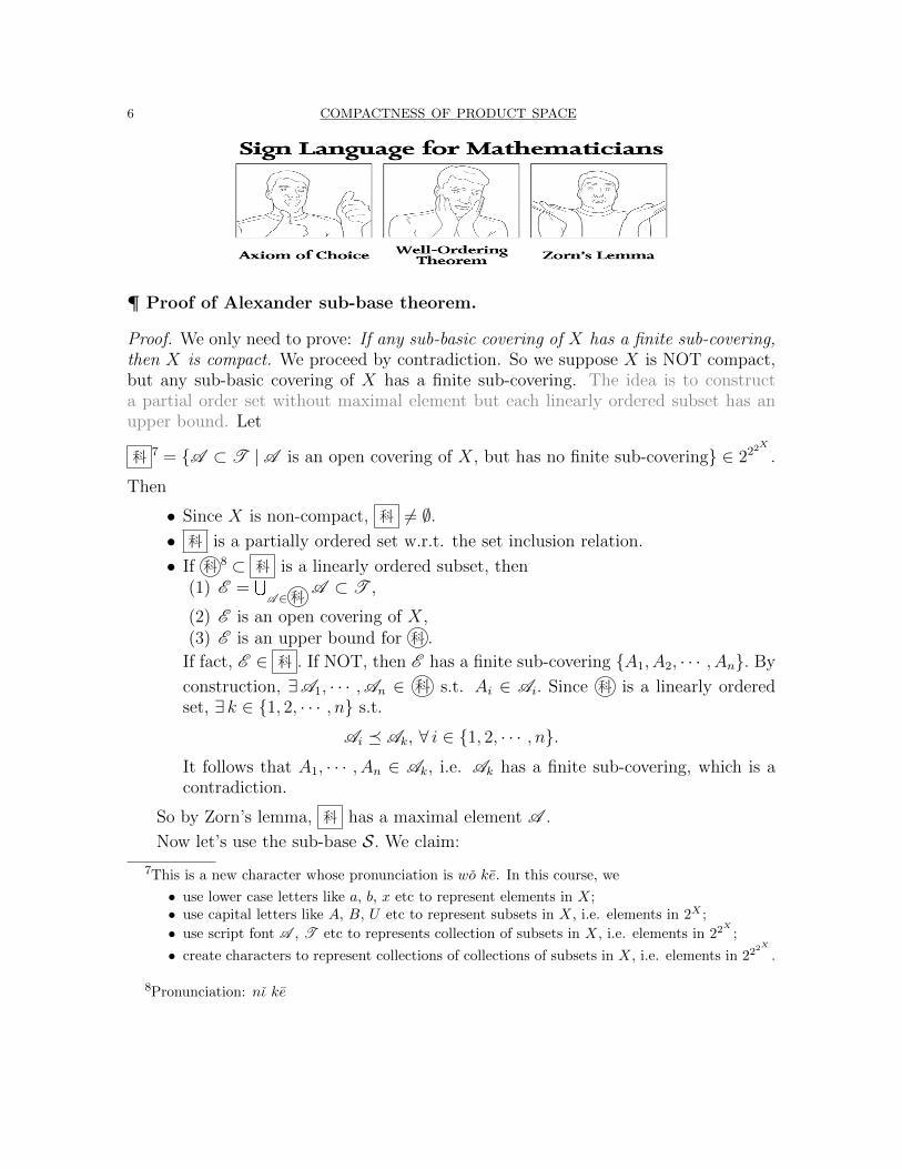
6 COMPACTNESS OF PRODUCT SPACE
¶ Proof of Alexander sub-base theorem.
Proof. We only need to prove: If any sub-basic covering of X has a finite sub-covering,then X is compact. We proceed by contradiction. So we suppose X is NOT compact,but any sub-basic covering of X has a finite sub-covering. The idea is to constructa partial order set without maximal element but each linearly ordered subset has anupper bound. Let
� 7 = {A ⊂ T |A is an open covering of X, but has no finite sub-covering} ∈ 222X
.
Then
• Since X is non-compact, � 6= ∅.• � is a partially ordered set w.r.t. the set inclusion relation.
• If � 8 ⊂ � is a linearly ordered subset, then(1) E =
SA ∈�
A ⊂ T ,
(2) E is an open covering of X,(3) E is an upper bound for � .
If fact, E ∈ � . If NOT, then E has a finite sub-covering {A1, A2, · · · , An}. By
construction, ∃A1, · · · ,An ∈ � s.t. Ai ∈ Ai. Since � is a linearly orderedset, ∃ k ∈ {1, 2, · · · , n} s.t.
Ai � Ak, ∀ i ∈ {1, 2, · · · , n}.It follows that A1, · · · , An ∈ Ak, i.e. Ak has a finite sub-covering, which is acontradiction.
So by Zorn’s lemma, � has a maximal element A .
Now let’s use the sub-base S. We claim:
7This is a new character whose pronunciation is wo ke. In this course, we
• use lower case letters like a, b, x etc to represent elements in X;• use capital letters like A, B, U etc to represent subsets in X, i.e. elements in 2X ;
• use script font A , T etc to represents collection of subsets in X, i.e. elements in 22X
;
• create characters to represent collections of collections of subsets in X, i.e. elements in 222X
.
8Pronunciation: nι ke
COMPACTNESS OF PRODUCT SPACE 7
Claim 1. S ∩A is an open covering of X.
First let’s suppose this is true. In other words, we get a covering S ∩ A of X.This covering can’t have finite sub-covering since A has no finite sub-covering. Buton the other hand, it must has a finite sub-covering since it is a sub-basic covering.Contradiction! This completes the proof. �
Proof of Claim 1. For any x ∈ X, ∃A ∈ A s.t. x ∈ A. By the definition of sub-base,∃S1, · · · , Sm ∈ S s.t. x ∈ S1 ∩ · · · ∩ Sm ⊂ A. We want to show that
∃ 1 ≤ k ≤ m s.t. Sk ∈ A .
(This implies Sk ∈ S ∩A and x ∈ Sk, so we are done.)
Again by contradiction. If NOT, Then for ∀ 1 ≤ k ≤ m,
Ak := A ∪ {Sk} � A .
Since A is a maximal element of � , we must have Ak /∈ � , i.e. Ak has a finitesub-covering {Sk, Ak,1, · · · , Ak,j(k)}, where Ak,j ∈ A . It follows that
X =m\k=1
(Sk ∪ Ak,1 ∪ · · · ∪ Ak,j(k)) = (S1 ∩ · · · ∩ Sm) ∪ ([k,j
Ak,j),
where we used the fact (A ∪B) ∩ (C ∪D) ⊂ (A ∩ C) ∪B ∪D. As a consequence,
{A,Ak,j | 1 ≤ k ≤ m, 1 ≤ j ≤ j(k)}is a finite sub-covering of A . Contradiction! �
¶ Tychonoff Theorem =⇒ Axiom of Choice.
So the main ingredient in the proof of Tychonoff theorem is the axiom of choice.One may ask: is it possible to prove Tychonoff theorem without using axiom of choice?The answer is no. In fact, Tychonoff theorem is equivalent to the axiom of choice:
Proposition 2.3 (Kelley: Tychonoff Theorem =⇒ Axiom of Choice).
Suppose Tychonoff Theorem is true, then (the equivalent statement of A.C.)
Xα 6= ∅,∀α =⇒Yα
Xα 6= ∅.
Proof. Each Xα is compact w.r.t. the trivial topology. Define fXα = Xα ∪ {∞α}, with
the topology gTα = {∅, Xα, {∞α}, gXα} which is still compact. By Tychonoff theorem,
X =QαfXα is compact w.r.t. the product topology.
Observation: {π−1α (Xα)} is a family of closed sets in X with F.I.P. (Why?)If follows from compactness that \
α
π−1α (Xα) 6= ∅.
By definition, any element in ∩απ−1α (Xα) is an element inQαXα. �
8 COMPACTNESS OF PRODUCT SPACE
3. Applications of Tychonoff Theorem
We shall give several applications of Tychonoff theorem.
¶ Application 1: Graph Coloring.
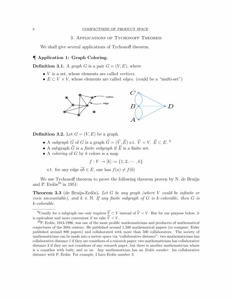
Definition 3.1. A graph G is a pair G = (V,E), where
• V is a set, whose elements are called vertices.• E ⊂ V × V, whose elements are called edges. (could be a “multi-set”)
Definition 3.2. Let G = (V,E) be a graph.
• A subgraph ÜG of G is a graph ÜG = (ÜV , ÜE) s.t. ÜV = V, ÜE ⊂ E. 9
• A subgraph ÜG is a finite subgraph if ÜE is a finite set.• A coloring of G by k colors is a map
f : V → [k] := {1, 2, · · · , k}
s.t. for any edge ab ∈ E, one has f(a) 6= f(b)
We use Tychonoff theorem to prove the following theorem proven by N. de Bruijnand P. Erdos10 in 1951:
Theorem 3.3 (de Bruijn-Erdos). Let G be any graph (where V could be infinite oreven uncountable), and k ∈ N. If any finite subgraph of G is k-colorable, then G isk-colorable.
9Usually for a subgraph one only requires ÜV ⊂ V instead of ÜV = V . But for our purpose below, it
is equivalent and more convenient if we take ÜV = V .10P. Erdos, 1913-1996, was one of the most prolific mathematicians and producers of mathematical
conjectures of the 20th century. He published around 1,500 mathematical papers (to compare: Eulerpublished around 800 papers) and collaborated with more than 500 collaborators. The society ofmathematicians can be made into a metric space via “collaborative distance”: two mathematicians hascollaborative distance 1 if they are coauthors of a research paper; two mathematicians has collaborativedistance 2 if they are not coauthors of any research paper, but there is another mathematician whoseis a coauthor with both; and so on. Any mathematician has an Erdos number : his collaborativedistance with P. Erdos. For example, I have Erdos number 3.
COMPACTNESS OF PRODUCT SPACE 9
Proof. Endow [k] = {1, 2, · · · , k} with the discrete topology and consider the product
X :=YV
[k] = {f : V → {1, 2, · · · , k}}.
Since [k] is compact, Tychonoff Theorem implies X is compact. For any subset F ⊂ E,we define
XF := {f : V → [k] | f is a coloring of (V, F )}.
Fact 1 If F = {ab} is a one-edge set, then XF is closed.
Reason: X{ab} = {f : V → [k] | f(a) 6= f(b)}
=[
1≤i 6=j≤k{f : V → [k] | f(a) = i, f(b) = j}
=[
1≤i 6=j≤k(π−1a (i) ∩ π−1b (j))
is a finite union of closed sets.
Fact 2 For any F ⊂ E, XF is closed.
Reason: XF1 ∩XF2 = XF1∪F2 =⇒ XF =\ab∈F
Xab
is an intersection of closed sets.
Now we consider the following collection of closed sets
F = {XF | F ⊂ E is a finite set}.We check that F satisfies F.I.P:
XF1 ∩XF2 ∩ · · · ∩XFn = XF1∪···∪Fm 6= ∅.(Since F1 ∪ · · · ∪ Fm is finite!) Since X is compact, we get\
XF∈F
XF 6= ∅.
But by definition, any element f ∈ ∩XF∈FXF is a k-coloring of G. �
As a consequence, the four-color theorem holds not only for finite planar graphs,but also for infinite graphs that can be drawn without crossings in the plane, and evenmore generally to infinite graphs (possibly with an uncountable number of vertices) forwhich every finite subgraph is planar!
10 COMPACTNESS OF PRODUCT SPACE
Reading:
¶ Application 2: Arithmetic progressions in subsets in Z.
We can also use topology to study number theory.
Definition 3.4. A partition of Z is a decomposition
Z = S1 ∪ · · · ∪ Sks.t. Si ∩ Sj = ∅ for i 6= j. [Equivalently, it is an k-coloring of Z (with no edges).]
Theorem 3.5 (Van der Waerden 1927). For any partition Z = S1 ∪ · · · ∪ Sk, ∃ j s.t.Sj contains arbitrary long (but still finite) arithmetic progressions.
Van der Waerden’s theorem is a precursor of the famous Szemerendi’s theorem:
Theorem 3.6 (Szemeredi, 1975). Any subset A ⊂ N with
lim supn→∞
|A ∩ {1, · · · , n}|n
> 0
contains infinitely many arithmetic progressions of length k for all positive integers k.
In 1977, Furstenberg11 gave an ergodic theory reformulation and obtained a proofusing topology, and then proved a multidimensional generalization of Szemeredi’s the-orem. In what follows we state a topological version of van der Waerden’s theorem,using which we prove the number-theoretic version.
Theorem 3.7 (Topological version of van der Waerden). Let X be compact, T : X →X be a homeomorphism, and {Vα} an open covering of X. Then ∀ l ∈ N, ∃n ∈ N andopen set V ∈ {Vα} s.t.
V ∩ T−nV ∩ · · · ∩ T−(l−1)nV 6= ∅.
Theorem 3.7 can be proven in the framework of general topology after introducingsome conceptions in the subject “topological dynamical system”, but we will omit that.In what follows we prove:
Theorem 3.7 ⇒ Theorem 3.5
Proof. Again endow [k] with the discrete topology. By Tychonoff, the space
fX =YZ
[k] = {f : Z→ [k]}
is compact. Note that any partition of Z corresponds to an element in fX.11H. Fursterberg is a famous American-Israeli mathematician who won Wolf prize in 2006/7 and
won Abel prize in 2020, for his “pioneering the use of methods from probability and dynamics ingroup theory, number theory and combinatorics”. You have seen his proof of the infinitude of primenumbers in PSet 2-1-2: the proof was published in 1955 when he was still an undergraduate studentin Yeshiva University.
COMPACTNESS OF PRODUCT SPACE 11
Let T : fX → fX be the “right-shift” map: T (f)(n) = f(n−1). Then T is continuoussince T−1(π−1n (i)) = π−1n−1(i), and {π−1n (i)} is a sub-base. Similarly T−1, the “left-shift”map, is continuous. So T is a homeomorphism.
Let f ∈ fX be the element that corresponds to the partition in Theorem 3.5. Let
X = {T nf | n ∈ Z} = {· · · , T−2f, T−1f, f, Tf, T 2f, · · · }
As a closed set in the compact spact fX, X itself is compact. Moreover, T (X) = X:
Reason: T (X) ⊃ {T nf | n ∈ Z} ⇒ T (X) ⊃ X.Replace T with T−1, we get T−1(X) ⊃ X.
So T : X → X is a homeomorphism. (Think of this: why?)
Now for each i ∈ [k], denote
Vi = {f ∈ fX | f(0) = i} = π−10 (i).
Then Vi’s are open in fX, and form an open covering of X. By Theorem 3.7, ∀ l ∈ N,∃n ∈ N and Vj ∈ {Vi | 1 ≤ i ≤ k} s.t.
(Vj ∩ T−nVj ∩ · · · ∩ T−(l−1)nVj) ∩X 6= ∅.
Note: Vj ∩ T−nVj ∩ · · · ∩ T−(l−1)nVj is open in fX, while X = {T−nf | n ∈ Z}. So thereexists m s.t.
T−mf ∈ Vj ∩ T−nVj ∩ · · · ∩ T−(l−1)nVj,i.e.
f ∈ TmVj ∩ Tm−nVj ∩ · · · ∩ Tm−(l−1)nVj.It follows
f(m) = f(m− n) = · · · = f(m− (l − 1)n) = j.
In other words, m,m− n, · · · ,m− (l − 1)n ∈ Sj. �
¶ Application 3: The Banach-Alaoglu theorem.
The third application is to functional analysis. Recall that a normed vector spaceis a vector space X endowed with a norm structure, i.e. a function ‖ · ‖ : X → [0,+∞)such that for any x, y ∈ X and any λ ∈ C,
• ‖x‖ ≥ 0, and ‖x‖ = 0⇔ x = 0;• ‖x+ y‖ ≤ ‖x‖+ ‖y‖;• ‖λx‖ = |λ|‖x‖.
On any normed vector space (X, ‖ · ‖), one can easily check that d(x, y) := ‖x − y‖defines a metric structure. So we can always endow X with the metric topology, andtalk about continuity of maps. In particular, we denote
X∗ := {l : X → C | l is complex linear and continuous}.
12 COMPACTNESS OF PRODUCT SPACE
The space X∗ is again a linear space, on which one can define a norm
‖l‖ := sup‖x‖=1
|l(x)|.
The new normed vector space (X∗, ‖ ·‖) is called the dual space of (X, ‖ ·‖). It is againa metric space and we can talk about conceptions like the closed unit ball,
B∗ := {l ∈ X∗ | ‖l‖ ≤ 1}.Unfortunately, in most applications, normed vector spaces and their dual spaces areinfinitely dimensional, and thus the closed unit ball are not compact with respect tothe usual metric topology.
Of course the reason for the non-compactness is that the metric topologies aretoo strong, i.e. they contain too much open sets. In Lecture 5 (Example 2.5) weintroduced two new topologies: the weak topology on X and the weak-∗ topology onX∗. The weak topology on X is the weakest topology making all linear functionalsl ∈ X∗ continuous, and the weak-∗ topology on X∗ is the weakest topology makingall evaluation maps evx continuous. From this definition it is quite easy to see thatthe weak-∗ topology is the pointwise convergence topology if we regard X∗ as a subsetof M(X,C). Since the pointwise convergence topology on M(X,C) can be identifiedwith the product topology on CX , it is not too surprising that the closed unit ball B∗
is closed with respec to the weak-∗ topology:
Theorem 3.8 (Banach-Alaoglu). Let X be a normed vector space. Then the closedunit ball B∗ in the dual space X∗ is compact with respect to the weak-∗ topology.
Proof. The idea is to identify the closed unit ball B∗ of X∗ with a closed subset of
Z =Yx∈X{z ∈ C | |z| ≤ ‖x‖} ⊂ CX ,
where Z is compact since we endow Z with the product topology.
As we explained above, we can identify X∗ with a subspace of M(X,C) and thusany element l ∈ X∗ satisfying ‖l‖ ≤ 1 can be identified with an element in Z. Con-versely, an element f in Z belongs to the closed unit ball B∗ in X∗ if and only if
f(x+ y) = f(x) + f(y) and f(λx) = λf(x)
for all x, y ∈ X and λ ∈ C. In other words, f ∈ B∗ if and only if, as an element of Z,it belongs to the set
D = {f ∈ Z | evx+y(f) = evx(f) + evy(f), evαx(f) = αevx(f),∀x, y ∈ X, ∀α ∈ C}=\x,y,α
(evx+y − evx − evy)−1(0) ∩ (evαx − αevx)
−1(0).
By continuity of the evaluation maps, D is a closed subset in Z. Since Z is compact, soisD. One can carefully check that the identification above is a homeomorphism between(B∗,Tweak∗) and (D,Tproducut). So B∗ is compact w.r.t. the weak-∗ topology. �