Compactness: a Mathematical IntroductionAnthony E. Pizzimenti

The University of Iowa Department of Mathematicsanthony-pizzimenti@uiowa.edu

Revised: January 5, 2021

A particularly consequential obsession has broken out among those whostudy gerrymandering: compactness. Its mathematical ambiguity, legalweight, and its lack of consistency is of much debate in the gerrymander-ing world. Here, we attempt to ground compactness’ vagueness in math-ematical rigor: to do so, we investigate a number of traditional compact-ness scores, as well as explore a specific set of alternative compactnessmeasures aimed at measuring non-convexity.

Contents1 Introduction 2

1.1 Vocabulary and Definitions . . . . . . . . . . . . . . . . . . . . . . 21.2 Traditional Compactness Scores . . . . . . . . . . . . . . . . . . . 4

2 Traditional Compactness Scores: a Closer Look 62.1 Polsby-Popper . . . . . . . . . . . . . . . . . . . . . . . . . . . . . . 62.2 Reock . . . . . . . . . . . . . . . . . . . . . . . . . . . . . . . . . . . 82.3 Convex Hull . . . . . . . . . . . . . . . . . . . . . . . . . . . . . . . 10

3 Measuring Non-Convexity 113.1 Angular Convexity . . . . . . . . . . . . . . . . . . . . . . . . . . . . 11

3.1.1 Parameterized Stepwise Function . . . . . . . . . . . . . . 153.1.2 Minimum Circular Contiguous Subarray Sum . . . . . . . 15

3.2 Cano Non-Convexity . . . . . . . . . . . . . . . . . . . . . . . . . . 163.2.1 Boundary Cano Non-convexity . . . . . . . . . . . . . . . . 18

4 Conclusions 19

1

1 IntroductionPartisan gerrymandering, as a practice, is not new. A deeply American politicaltactic, it has survived generations; after a particularly high-profile resurgencein the early 2010s, legal scholars, left-leaning politicians, activists, and math-ematicians began to fight back. Unfortunately, none of these fields of studyentirely capture gerrymandering’s complexity and nuance: it is, by nature, amulti-faceted issue which requires close looks from legal, mathematical, politi-cal, and racial standpoints. In this paper, we focus primarily on the relationshipbetweenmathematics and gerrymandering, andmore specifically, how to practi-cally operationalize the ambiguous legal concept of compactness, the connectionbetween legal compactness and geometric convexity, the pitfalls of this connec-tion, and how we may implement better measures of non-convexity in practice.

1.1 Vocabulary and DefinitionsWhen reading this text, it is important to keep in mind that many of the termslegal scholars use in practice have wildly different definitions than the sameterms’ definitions in mathematics. In order to prevent as much confusion aspossible, as well as lay out foundational concepts for the remainder of this paper,we give the following. Assume that any topological space discussed is at leastHausdorff.

Definition 1 (Interior, boundary, closure). Given some topologicalspace X and a subset S ⊆ X, denote S’s interior points by int{S},its boundary points by ∂S, and its closure by cl{S} = int{S}∪∂S.

Typically, any of the spaces X referred to later are either R2 or S2.

Definition 2 (State, subdivision). Given some space X, a state isa closed, path-connected subset S ⊆ X such that ∂S is a rectifiablecurve. Furthermore, we can write S as

S =⋃i∈I

cl{s}i, I = {1, . . . , n},

where each si is itself an open subset of X called a subdivisionsuch that si ∩ sj = ∅ for i 6= j and each ∂si is a rectifiable curve.Here, we write S = {si}i∈I for convenience.

Oftentimes the chunking-up of a state, as laid out in Definition 2, is erroneouslyreferred to as a partition. While this may make sense intuitively, it is – math-

2

ematically – not the case. The cover formed by the set {cl{si}}i∈I is not a par-tition, as it is possible for a single point to lie on the boundary of si and sj evenif i 6= j. However, if we consider the collection (si)i∈I and the set of all boundarypoints B =

⋃i∈I si, then the family of sets ((si)i∈I , B) is a partition, as every

point lies in exactly one of the si (by Def. 2) or on the boundary of one of the si.

While the study of gerrymandering, at its face, deals primarily in topology, manyproperties of import can be studied in an equivalent but simpler environmentusing the notion of duality. These properties – like perimeter, area, member-ship (of political and geographic region), population, adjacency, and more – canbe encoded in a data structure called a graph, where graphs are structurescomposed of vertices (nodes) and edges1.

Definition 3 (Dual graph). Let the set V be a set of vertices {vi}i∈I .Now, we define fV : S → V such that fV (si) = vi. Now, let E be a setof edges {(vi, vj)}i 6=j∈I , and define the function fE : S × S → E suchthat

fE(si, sj) =

{(fV (si), fV (sj)) i 6= j and |∂si ∩ ∂sj | > 1

∅ otherwise.

Then, the graph GS = (V,E) is considered the dual graph of S.

This definition of a dual graph prevents self-loops, and draws edges betweenpairs of vertices if the duals of the vertices in the pair are adjacent. In practice,we determine the embedding of GS in R2 (or S2) by embedding each vertex viat the centroid of si, with edges (vi, vj) embedded as segments whose endpointsare at the centroids of si and sj , respectively.

This application of duality is quite fruitful: in practice, the geometric data ofeach subdivision are stored as polygons, and other data stored as attributes ofthe polygon. By discretizing our geographic data in this way, we avoid theunnecessary and expensive computation required to store and operate on ex-tremely large sets of polygons. While this discretization necessarily loses someof the geographic detail, finer subdivisions (i.e. more, smaller chunks) of thestate will produce a dual graph with an embedding which captures much of theoriginal geography.

1The internet is an example of a real-world graph: websites are the vertices (nodes), and twowebsites have an edge between them if you can get from each website to the other in one hop.

3

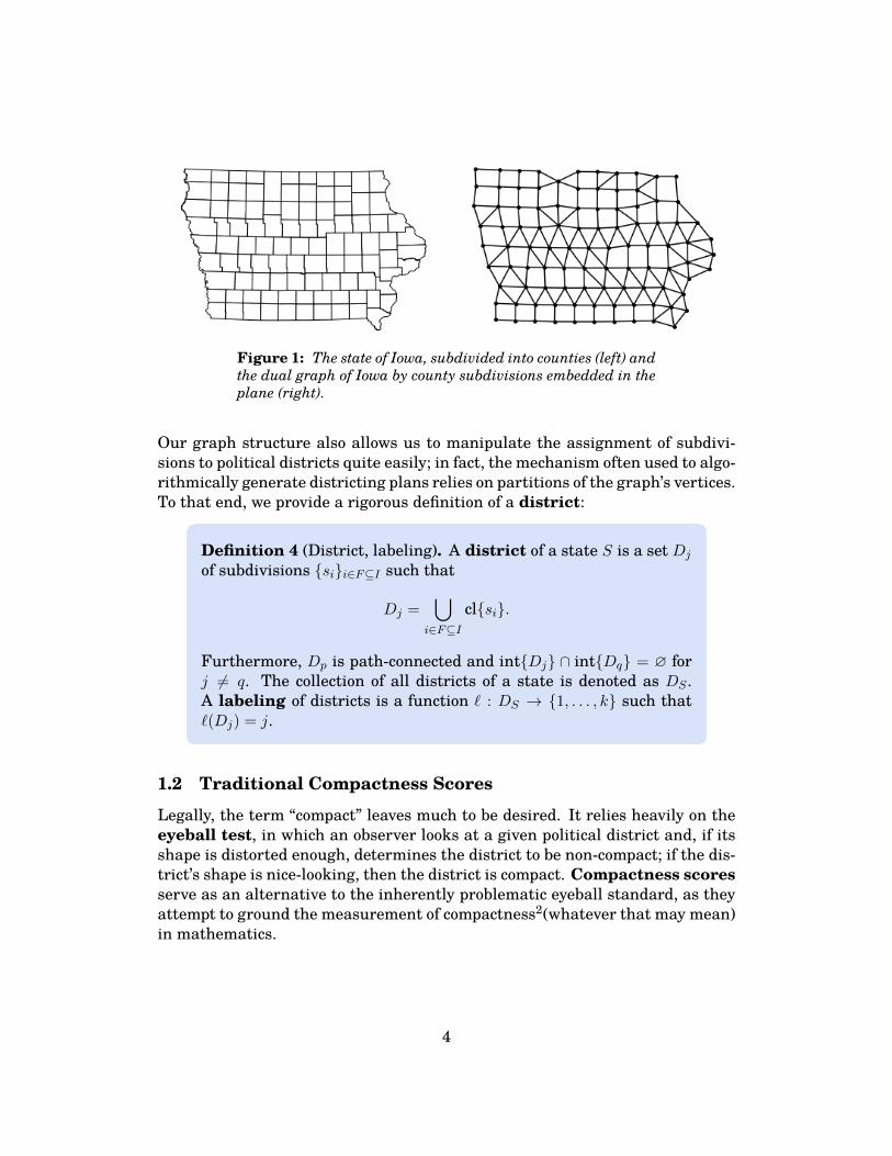
Figure 1: The state of Iowa, subdivided into counties (left) andthe dual graph of Iowa by county subdivisions embedded in theplane (right).

Our graph structure also allows us to manipulate the assignment of subdivi-sions to political districts quite easily; in fact, the mechanism often used to algo-rithmically generate districting plans relies on partitions of the graph’s vertices.To that end, we provide a rigorous definition of a district:

Definition 4 (District, labeling). A district of a state S is a set Dj

of subdivisions {si}i∈F⊆I such that

Dj =⋃

i∈F⊆Icl{si}.

Furthermore, Dp is path-connected and int{Dj} ∩ int{Dq} = ∅ forj 6= q. The collection of all districts of a state is denoted as DS .A labeling of districts is a function ` : DS → {1, . . . , k} such that`(Dj) = j.

1.2 Traditional Compactness ScoresLegally, the term “compact” leaves much to be desired. It relies heavily on theeyeball test, in which an observer looks at a given political district and, if itsshape is distorted enough, determines the district to be non-compact; if the dis-trict’s shape is nice-looking, then the district is compact. Compactness scoresserve as an alternative to the inherently problematic eyeball standard, as theyattempt to ground the measurement of compactness2(whatever that may mean)in mathematics.

4

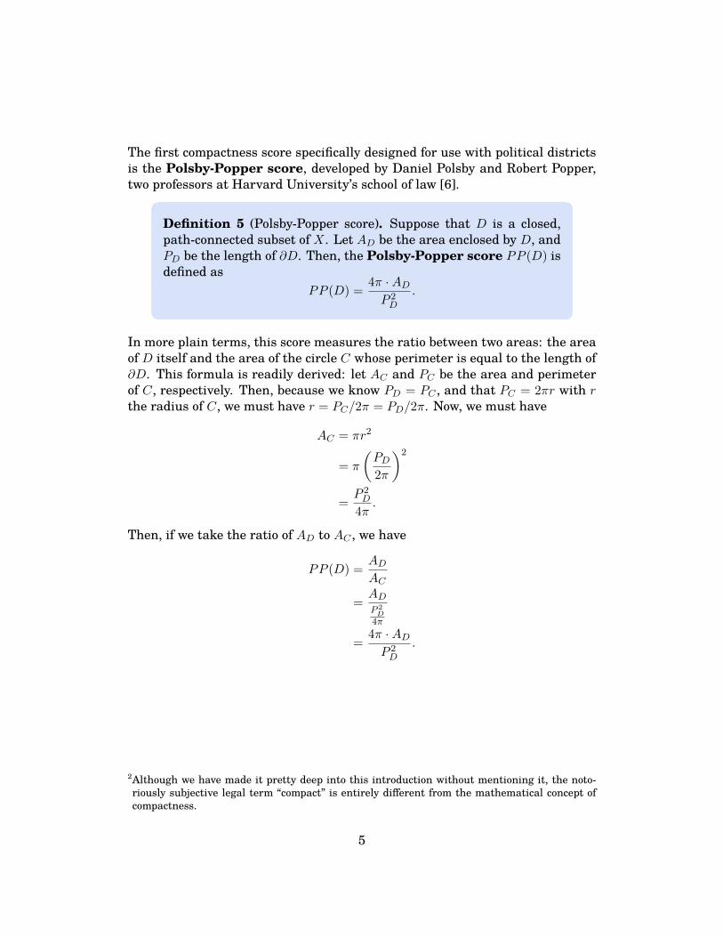
The first compactness score specifically designed for use with political districtsis the Polsby-Popper score, developed by Daniel Polsby and Robert Popper,two professors at Harvard University’s school of law [6].

Definition 5 (Polsby-Popper score). Suppose that D is a closed,path-connected subset of X. Let AD be the area enclosed by D, andPD be the length of ∂D. Then, the Polsby-Popper score PP (D) isdefined as

PP (D) =4π ·ADP 2D

.

In more plain terms, this score measures the ratio between two areas: the areaof D itself and the area of the circle C whose perimeter is equal to the length of∂D. This formula is readily derived: let AC and PC be the area and perimeterof C, respectively. Then, because we know PD = PC , and that PC = 2πr with rthe radius of C, we must have r = PC/2π = PD/2π. Now, we must have

AC = πr2

= π

(PD2π

)2

=P 2D

4π.

Then, if we take the ratio of AD to AC , we have

PP (D) =ADAC

=ADP 2D

4π

=4π ·ADP 2D

.

2Although we have made it pretty deep into this introduction without mentioning it, the noto-riously subjective legal term “compact” is entirely different from the mathematical concept ofcompactness.

5

We define the Reock score similarly [7]:

Definition 6 (Reock score). Suppose thatD is as inDefinition 5. LetAD be the area enclosed by D, and let C be the minimum boundingcircle of D, with AC its area. Then, the Reock score is defined as

Reock(D) =ADAC

.

Again, we take the ratio of two areas: the ratio of the D’s area to that of itsminimum bounding circle’s. Finally, we define the last compactness score weconsider: the Convex Hull score.

Definition 7 (ConvexHull score). Suppose thatD is as in Definition5. Let AD be the area enclosed by D, and let H be the convex hull ofD with AH its area. Then, the Convex Hull score is defined as

CH(D) =ADAH

.

Again a ratio of areas, this score brings us the closest to a measure of mathe-matical convexity. Conveniently, each of these scores gives a numerical resultin the range [0, 1], with 1 being an “optimally-shaped” district (according to themeasure) while anything close to 0 is non-optimal.

2 Traditional Compactness Scores: a Closer LookNow, we aim to investigate each of the three traditional compactness scores –Polsby-Popper, Reock, and Convex Hull – individually.

2.1 Polsby-PopperThe Polsby-Popper score is founded on the isoperimetric inequality, whichstates, for a given district D, that

P 2D ≥ 4π ·AD,

with PD and AD defined as before. Equality in the above expression only holdswhenD is a circle; thus, Polsby-Popper favors shapesDwhose squared-perimeter-to-area ratio is close to 4π. Lastly, As Polsby-Popper is area-comparative, thescore always falls in the range [0, 1].

6

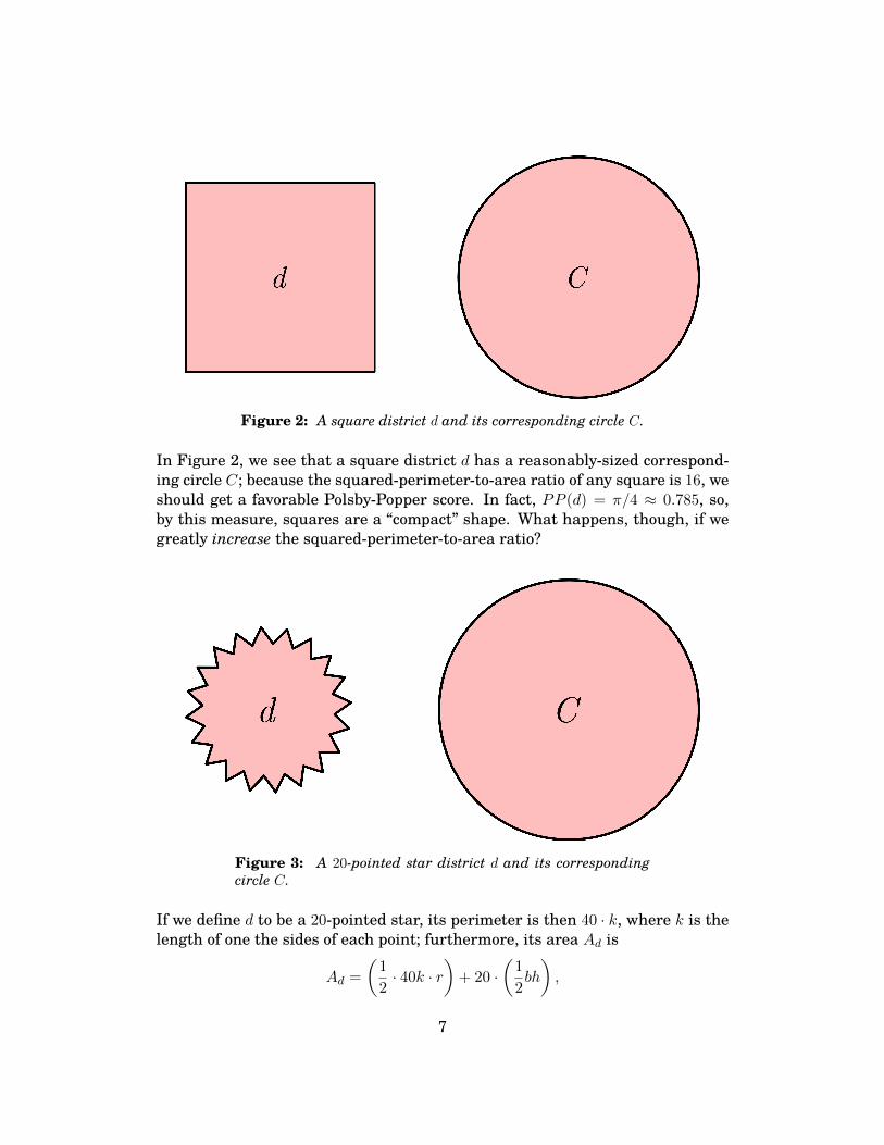
Figure 2: A square district d and its corresponding circle C.

In Figure 2, we see that a square district d has a reasonably-sized correspond-ing circle C; because the squared-perimeter-to-area ratio of any square is 16, weshould get a favorable Polsby-Popper score. In fact, PP (d) = π/4 ≈ 0.785, so,by this measure, squares are a “compact” shape. What happens, though, if wegreatly increase the squared-perimeter-to-area ratio?

Figure 3: A 20-pointed star district d and its correspondingcircle C.

If we define d to be a 20-pointed star, its perimeter is then 40 · k, where k is thelength of one the sides of each point; furthermore, its area Ad is

Ad =

(1

2· 40k · r

)+ 20 ·

(1

2bh

),

7

where r is the radius of d’s inscribed circle, and b and h are the base and heightof one of the triangular points. If we let k = 1 and r = 2, then our squared-perimeter-to-area ratio is 32, a significant deviation from the desired ratio of 4π.This deviation explains the poor score d receives – PP (d) ≈ 0.579.

In Figures 2 and 3 we can see that the Polsby-Popper is quite sensitive, espe-cially when boundaries are ragged. According to this score, the best possibleshape is a perfect circle; significant deviations from its ideal ratio of 4π are pun-ished heavily, even when a shape – like the 20-pointed star – looks quite close toa circle. Furthermore, this score’s implication that a circle is the ideal districtshape is impractical: even if the circles are of different sizes, a finite number ofcircular districts cannot form an interior-disjoint covering of a state.

In practice, individual subdivisions are stored as separate polygons, and largerobjects – like districts or states – are simply unions of these smaller polygonscalled multipolygons. Both polygons and multipolygons store a number of at-tributes, including area and perimeter: to calculate area and perimeter, poly-gons require a preprocessing step linear in the number of vertices, and multi-polygons require a preprocessing step linear in the number of polygons. How-ever, as Polsby-Popper relies exclusively on the properties of the (multi)polygon,this score can be computed in constant time.

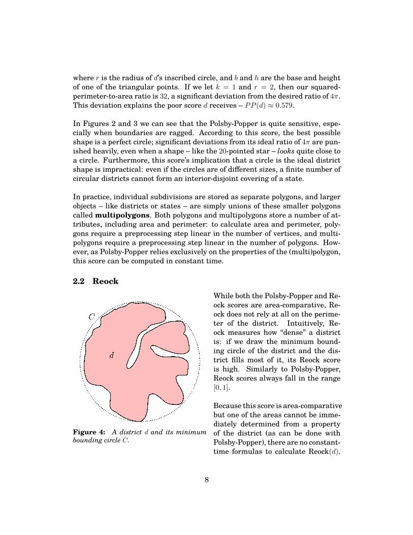
2.2 Reock

Figure 4: A district d and its minimumbounding circle C.

While both the Polsby-Popper and Re-ock scores are area-comparative, Re-ock does not rely at all on the perime-ter of the district. Intuitively, Re-ock measures how “dense” a districtis: if we draw the minimum bound-ing circle of the district and the dis-trict fills most of it, its Reock scoreis high. Similarly to Polsby-Popper,Reock scores always fall in the range[0, 1].

Because this score is area-comparativebut one of the areas cannot be imme-diately determined from a propertyof the district (as can be done withPolsby-Popper), there are no constant-time formulas to calculate Reock(d).

8

In practice, we can use a conventional minimum bounding disk-finding algo-rithm to find C and calculate the area of d conventionally as well [3]. In thecase above, Reock(d) ≈ 0.7697, which tells us that the district d is reasonablycompact.

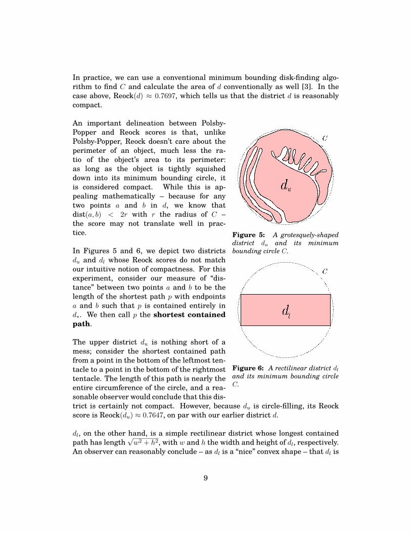
Figure 5: A grotesquely-shapeddistrict du and its minimumbounding circle C.

Figure 6: A rectilinear district dland its minimum bounding circleC.

An important delineation between Polsby-Popper and Reock scores is that, unlikePolsby-Popper, Reock doesn’t care about theperimeter of an object, much less the ra-tio of the object’s area to its perimeter:as long as the object is tightly squisheddown into its minimum bounding circle, itis considered compact. While this is ap-pealing mathematically – because for anytwo points a and b in d, we know thatdist(a, b) < 2r with r the radius of C –the score may not translate well in prac-tice.

In Figures 5 and 6, we depict two districtsdu and dl whose Reock scores do not matchour intuitive notion of compactness. For thisexperiment, consider our measure of “dis-tance” between two points a and b to be thelength of the shortest path p with endpointsa and b such that p is contained entirely ind∗. We then call p the shortest containedpath.

The upper district du is nothing short of amess; consider the shortest contained pathfrom a point in the bottom of the leftmost ten-tacle to a point in the bottom of the rightmosttentacle. The length of this path is nearly theentire circumference of the circle, and a rea-sonable observer would conclude that this dis-trict is certainly not compact. However, because du is circle-filling, its Reockscore is Reock(du) ≈ 0.7647, on par with our earlier district d.

dl, on the other hand, is a simple rectilinear district whose longest containedpath has length

√w2 + h2, with w and h the width and height of dl, respectively.

An observer can reasonably conclude – as dl is a “nice” convex shape – that dl is

9

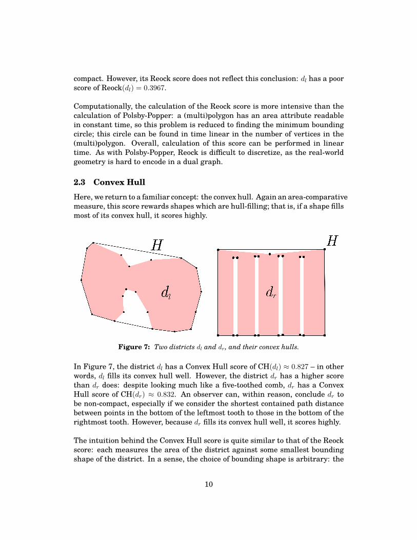
compact. However, its Reock score does not reflect this conclusion: dl has a poorscore of Reock(dl) = 0.3967.

Computationally, the calculation of the Reock score is more intensive than thecalculation of Polsby-Popper: a (multi)polygon has an area attribute readablein constant time, so this problem is reduced to finding the minimum boundingcircle; this circle can be found in time linear in the number of vertices in the(multi)polygon. Overall, calculation of this score can be performed in lineartime. As with Polsby-Popper, Reock is difficult to discretize, as the real-worldgeometry is hard to encode in a dual graph.

2.3 Convex HullHere, we return to a familiar concept: the convex hull. Again an area-comparativemeasure, this score rewards shapes which are hull-filling; that is, if a shape fillsmost of its convex hull, it scores highly.

Figure 7: Two districts dl and dr, and their convex hulls.

In Figure 7, the district dl has a Convex Hull score of CH(dl) ≈ 0.827 – in otherwords, dl fills its convex hull well. However, the district dr has a higher scorethan dr does: despite looking much like a five-toothed comb, dr has a ConvexHull score of CH(dr) ≈ 0.832. An observer can, within reason, conclude dr tobe non-compact, especially if we consider the shortest contained path distancebetween points in the bottom of the leftmost tooth to those in the bottom of therightmost tooth. However, because dr fills its convex hull well, it scores highly.

The intuition behind the Convex Hull score is quite similar to that of the Reockscore: each measures the area of the district against some smallest boundingshape of the district. In a sense, the choice of bounding shape is arbitrary: the

10

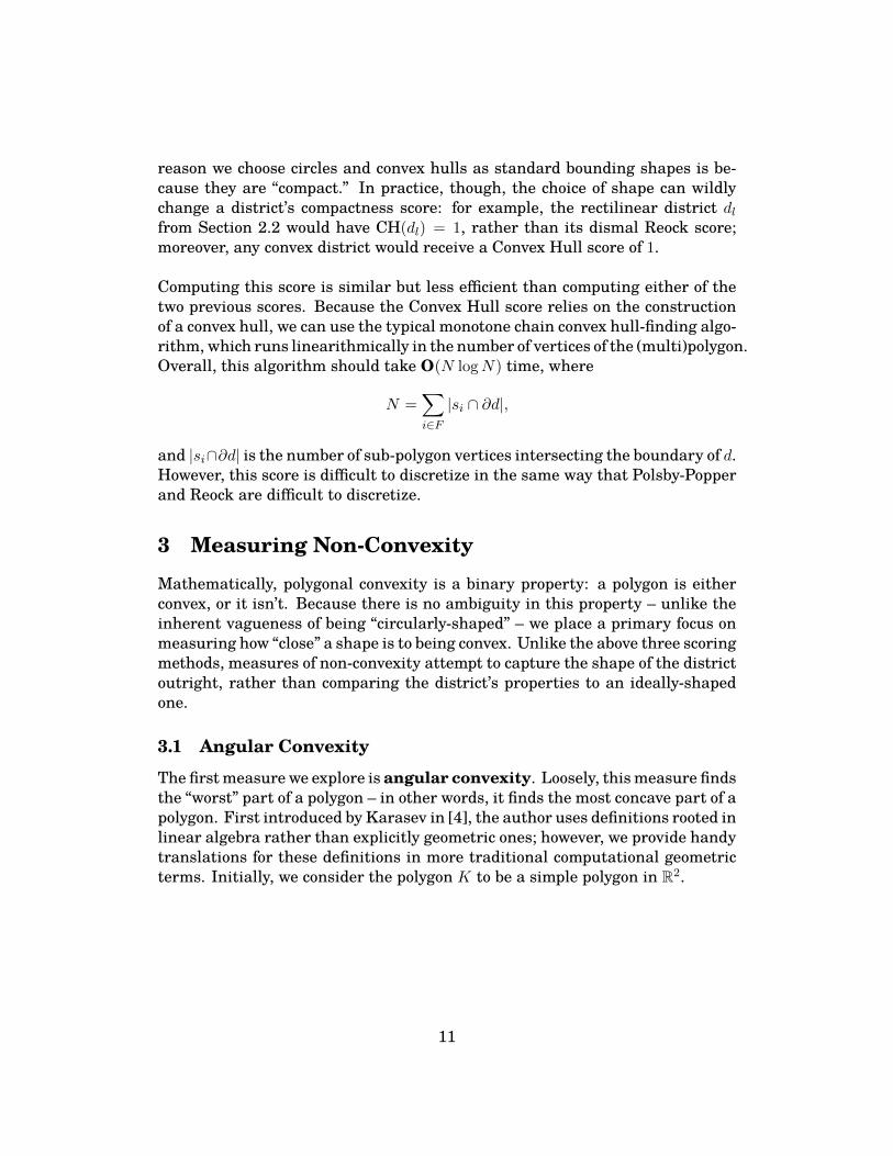
reason we choose circles and convex hulls as standard bounding shapes is be-cause they are “compact.” In practice, though, the choice of shape can wildlychange a district’s compactness score: for example, the rectilinear district dlfrom Section 2.2 would have CH(dl) = 1, rather than its dismal Reock score;moreover, any convex district would receive a Convex Hull score of 1.

Computing this score is similar but less efficient than computing either of thetwo previous scores. Because the Convex Hull score relies on the constructionof a convex hull, we can use the typical monotone chain convex hull-finding algo-rithm, which runs linearithmically in the number of vertices of the (multi)polygon.Overall, this algorithm should take O(N logN) time, where

N =∑i∈F|si ∩ ∂d|,

and |si∩∂d| is the number of sub-polygon vertices intersecting the boundary of d.However, this score is difficult to discretize in the same way that Polsby-Popperand Reock are difficult to discretize.

3 Measuring Non-ConvexityMathematically, polygonal convexity is a binary property: a polygon is eitherconvex, or it isn’t. Because there is no ambiguity in this property – unlike theinherent vagueness of being “circularly-shaped” – we place a primary focus onmeasuring how “close” a shape is to being convex. Unlike the above three scoringmethods, measures of non-convexity attempt to capture the shape of the districtoutright, rather than comparing the district’s properties to an ideally-shapedone.

3.1 Angular ConvexityThe firstmeasure we explore is angular convexity. Loosely, thismeasure findsthe “worst” part of a polygon – in other words, it finds the most concave part of apolygon. First introduced by Karasev in [4], the author uses definitions rooted inlinear algebra rather than explicitly geometric ones; however, we provide handytranslations for these definitions in more traditional computational geometricterms. Initially, we consider the polygon K to be a simple polygon in R2.

11

Definition 8 (Polyline). Let the sequence of points (v1, . . . , vn) bethe set of vertices for K in counterclockwise order; as K is closed,we note that v1 = vn, and index vertices modulo n. Then, the poly-line P is the sequence of vertices paired with the sequence of edges(v1v2, . . . , vn−1vn).

Based on this definition, we can conclude that simple polygons are uniquelydetermined by their polylines (up to translation and rotation).

Definition 9 (Shift sequence). Consider the polyline P and the se-quence of vertices (v1, . . . , vn). The shift sequence of P , denotedS(P ), is the sequence of vectors (v2 − v1, . . . , vn − vn−1). For conve-nience, we write S(P ) = (s1, . . . , sn), with si = vi+1 − vi.

Intuitively, this sequence of vectors traces out the shape of the polygon in theplane when the vectors are placed tip-to-tail in counter-clockwise order.

Definition 10 (Skew product, parallel, opposite). Given two vectorsu and v in R2, the skew product [◦, ◦] : R2 × R2 → R is defined as

[u, v] = uxvy − uyvx.

Two vectors are considered parallel if v = αu, and opposite ifthey are parallel but α < 0. In other words, two linearly dependentvectors u and v are parallel if v = αu with α ≥ 0, and oppositeotherwise.

This skew product, of course, can be equivalently formulated as the determi-nant of the matrix A =

[u v

], and this determinant is 0 if u and v are linearly

dependent. Now, we define the key measure underpinning angular convexity:

12

Definition 11 (Angle, rotation). The angle between two vectors uand v is denoted by ∠(u, v). This angle is signed positive if [u, v] > 0and negative if [u, v] < 0. Then, given a polyline P (where, wlog,S(P ) does not contain a pair of parallel or opposite vectors) the ro-tation of P is defined to be

rot(P ) = rot(S(P )) =n∑i=1

∠(si, si+1).

Additionally, the angle can be determined using the definition of the dot product:

∠(si, si+1) = sgn([si, si+1]) · cos−1(

si · si+1

‖si‖‖si+1‖

).

This calculation does two things: firstly, it finds the exterior angle at the vertexvi+1 (the point at which si ends and si+1 begins); secondly, it determines whethervi+1 is a reflex or convex vertex.

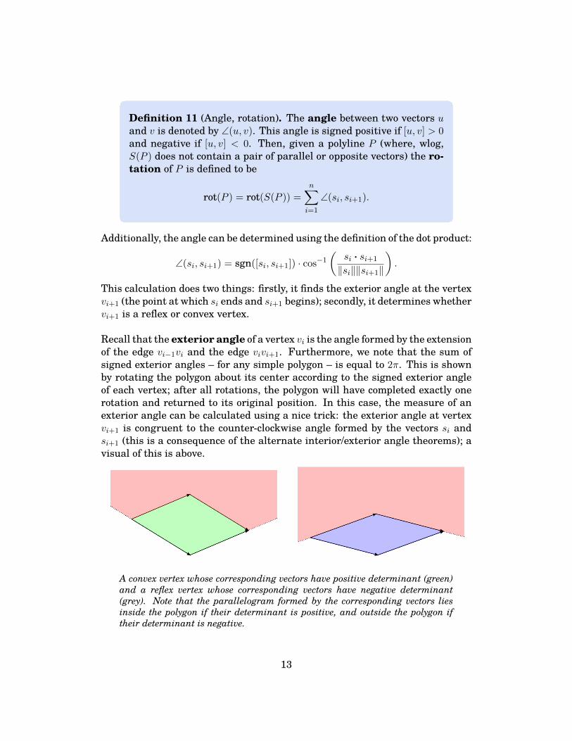
Recall that the exterior angle of a vertex vi is the angle formed by the extensionof the edge vi−1vi and the edge vivi+1. Furthermore, we note that the sum ofsigned exterior angles – for any simple polygon – is equal to 2π. This is shownby rotating the polygon about its center according to the signed exterior angleof each vertex; after all rotations, the polygon will have completed exactly onerotation and returned to its original position. In this case, the measure of anexterior angle can be calculated using a nice trick: the exterior angle at vertexvi+1 is congruent to the counter-clockwise angle formed by the vectors si andsi+1 (this is a consequence of the alternate interior/exterior angle theorems); avisual of this is above.

A convex vertex whose corresponding vectors have positive determinant (green)and a reflex vertex whose corresponding vectors have negative determinant(grey). Note that the parallelogram formed by the corresponding vectors liesinside the polygon if their determinant is positive, and outside the polygon iftheir determinant is negative.

13

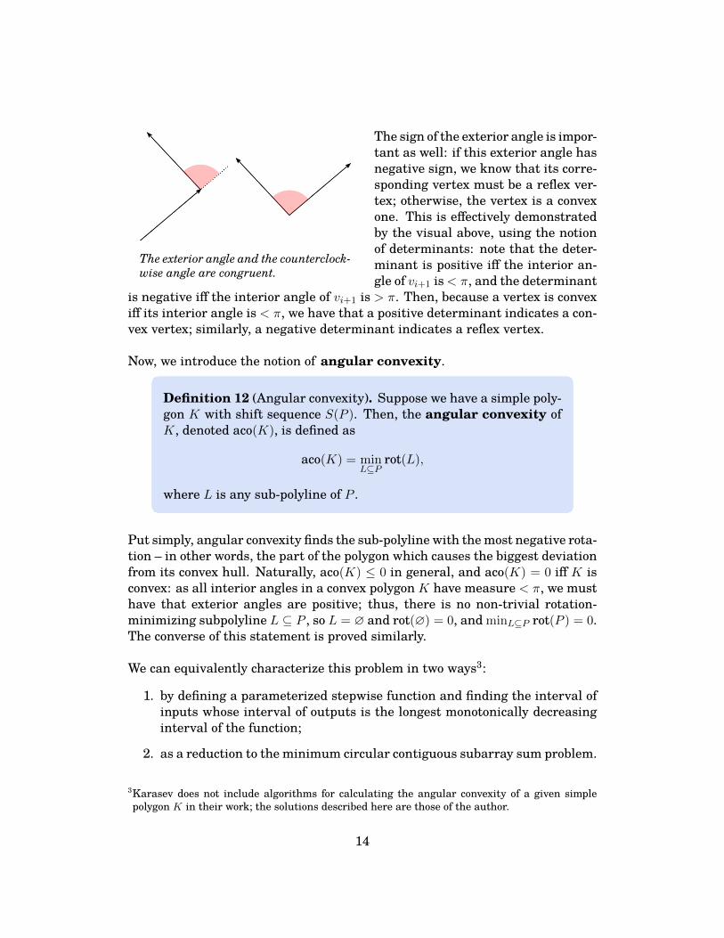
The exterior angle and the counterclock-wise angle are congruent.

The sign of the exterior angle is impor-tant as well: if this exterior angle hasnegative sign, we know that its corre-sponding vertex must be a reflex ver-tex; otherwise, the vertex is a convexone. This is effectively demonstratedby the visual above, using the notionof determinants: note that the deter-minant is positive iff the interior an-gle of vi+1 is< π, and the determinant

is negative iff the interior angle of vi+1 is > π. Then, because a vertex is convexiff its interior angle is < π, we have that a positive determinant indicates a con-vex vertex; similarly, a negative determinant indicates a reflex vertex.

Now, we introduce the notion of angular convexity.

Definition 12 (Angular convexity). Suppose we have a simple poly-gon K with shift sequence S(P ). Then, the angular convexity ofK, denoted aco(K), is defined as

aco(K) = minL⊆P

rot(L),

where L is any sub-polyline of P .

Put simply, angular convexity finds the sub-polyline with themost negative rota-tion – in other words, the part of the polygon which causes the biggest deviationfrom its convex hull. Naturally, aco(K) ≤ 0 in general, and aco(K) = 0 iff K isconvex: as all interior angles in a convex polygonK have measure < π, we musthave that exterior angles are positive; thus, there is no non-trivial rotation-minimizing subpolyline L ⊆ P , so L = ∅ and rot(∅) = 0, andminL⊆P rot(P ) = 0.The converse of this statement is proved similarly.

We can equivalently characterize this problem in two ways3:

1. by defining a parameterized stepwise function and finding the interval ofinputs whose interval of outputs is the longest monotonically decreasinginterval of the function;

2. as a reduction to the minimum circular contiguous subarray sum problem.

3Karasev does not include algorithms for calculating the angular convexity of a given simplepolygon K in their work; the solutions described here are those of the author.

14

3.1.1 Parameterized Stepwise Function

First, we define our parameterized stepwise function f : I → R, where ourparameter t is a vertex’s index:

f(t) =t∑i=1

∠(si, si+1)

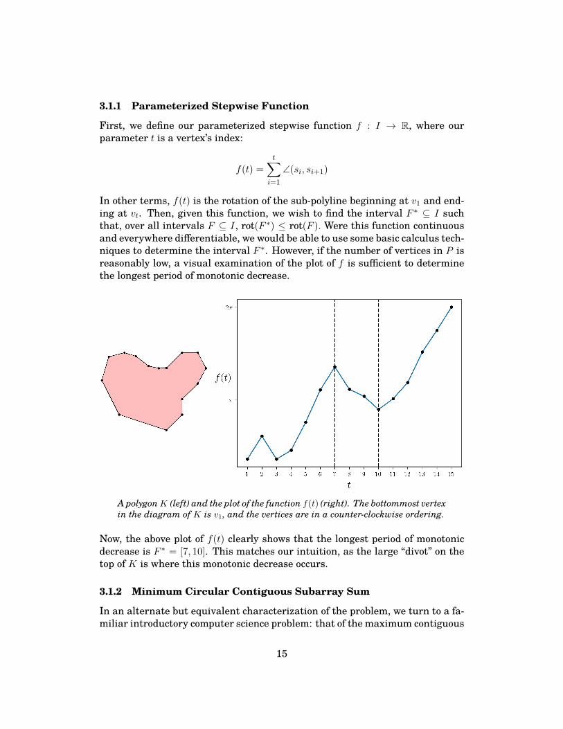
In other terms, f(t) is the rotation of the sub-polyline beginning at v1 and end-ing at vt. Then, given this function, we wish to find the interval F ∗ ⊆ I suchthat, over all intervals F ⊆ I, rot(F ∗) ≤ rot(F ). Were this function continuousand everywhere differentiable, we would be able to use some basic calculus tech-niques to determine the interval F ∗. However, if the number of vertices in P isreasonably low, a visual examination of the plot of f is sufficient to determinethe longest period of monotonic decrease.

A polygonK (left) and the plot of the function f(t) (right). The bottommost vertexin the diagram of K is v1, and the vertices are in a counter-clockwise ordering.

Now, the above plot of f(t) clearly shows that the longest period of monotonicdecrease is F ∗ = [7, 10]. This matches our intuition, as the large “divot” on thetop of K is where this monotonic decrease occurs.

3.1.2 Minimum Circular Contiguous Subarray Sum

In an alternate but equivalent characterization of the problem, we turn to a fa-miliar introductory computer science problem: that of the maximum contiguous

15

subarray sum. In this case, however, we wish to find the minimum contiguoussubarray sum, and, because the starting vertex on the polygon is arbitrary, wemust allow for circular sums: that is, sums whose terms may be on oppositeends of the array.

Let the arrayA contain the signed angles∠(si, si+1) such thatA[i−1] = ∠(si−1, si).Then, by the definition of angular convexity, we can calculate aco(K) by findingthe minimum circular contiguous subarray sum of A. Calculating this circularcontiguous sum is relatively simple, and can be implemented in time linear inthe number of K ’s vertices.Overall, thismeasure of non-convexity can be implemented using a simple linear-time algorithm. Additionally, it effectively captures the “shape” of a districtwithout comparison to some bounding shape, as Reock and Convex Hull do;angular convexity, then, provides a distinct advantage over area-comparativescores. A drawback, however, is the odd range of output values: while othermeasures score their districts in the range [0, 1], angular convexity has no well-defined lower bound, and the best districts – those that are convex – receive ascore of 0.

3.2 Cano Non-ConvexityThis measure of non-convexity, originally proposed by Cano, is surprising inits simplicity. It is neither a rotation-based nor area-comparative measure, asangular convexity and traditional compactness scores are; rather, it finds theHausdorff distance from a polygon K to its convex hull H. While the resultsof this paper primarily concern sets in Banach spaces, we note that Euclideanspace is, definitionally, a Banach space [2].

Definition 13 (Hausdorff distance). Let (M,d) be a metric space;let A and B be subsets of M . Then, the Hausdorff distance fromA to B is defined as

h(A,B) = supa∈A

{infb∈B{d(a, b)}

}.

Intuitively, this finds the longest of all shortest distances frompointsin A to points in B.

Now, we can formally define Cano non-convexity:

16

Definition 14 (Cano non-convexity). Let A ⊂ M with M a metricspace. Then, the Cano non-convexity of A is defined as

β(A) = h(A, conv(A)),

with conv(A) the convex hull of A [2]. If we wish to work exclusivelyin R2, we setM = R2.

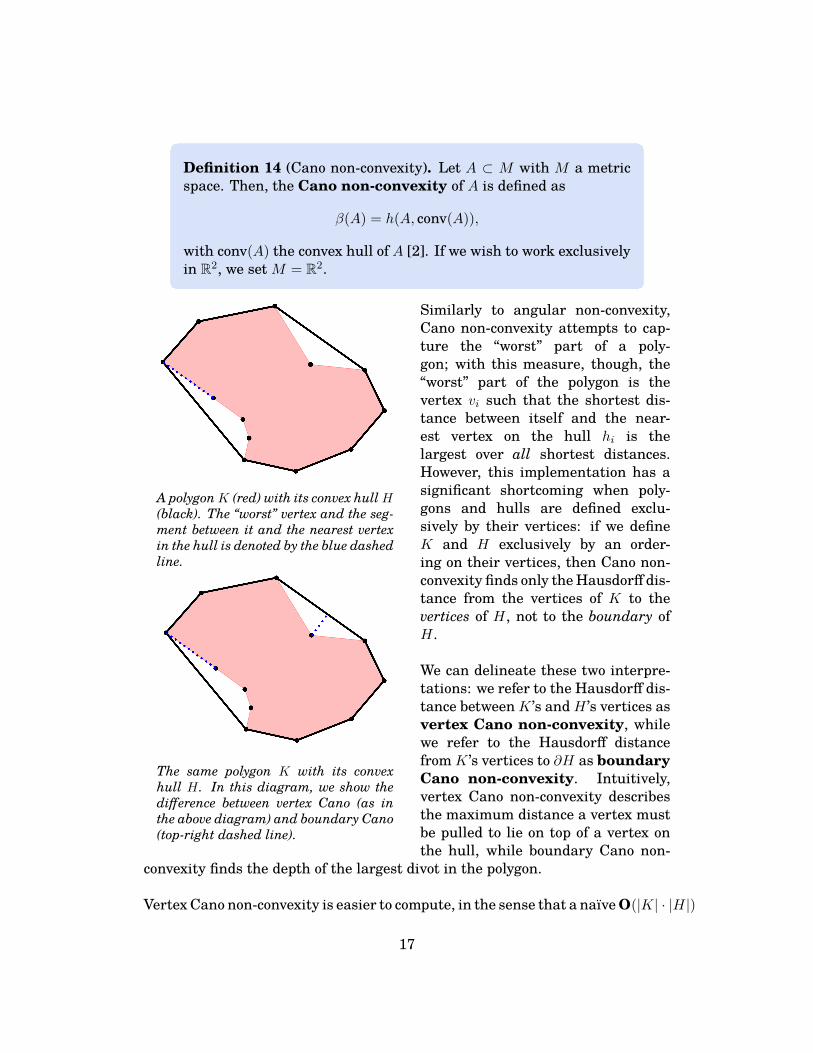
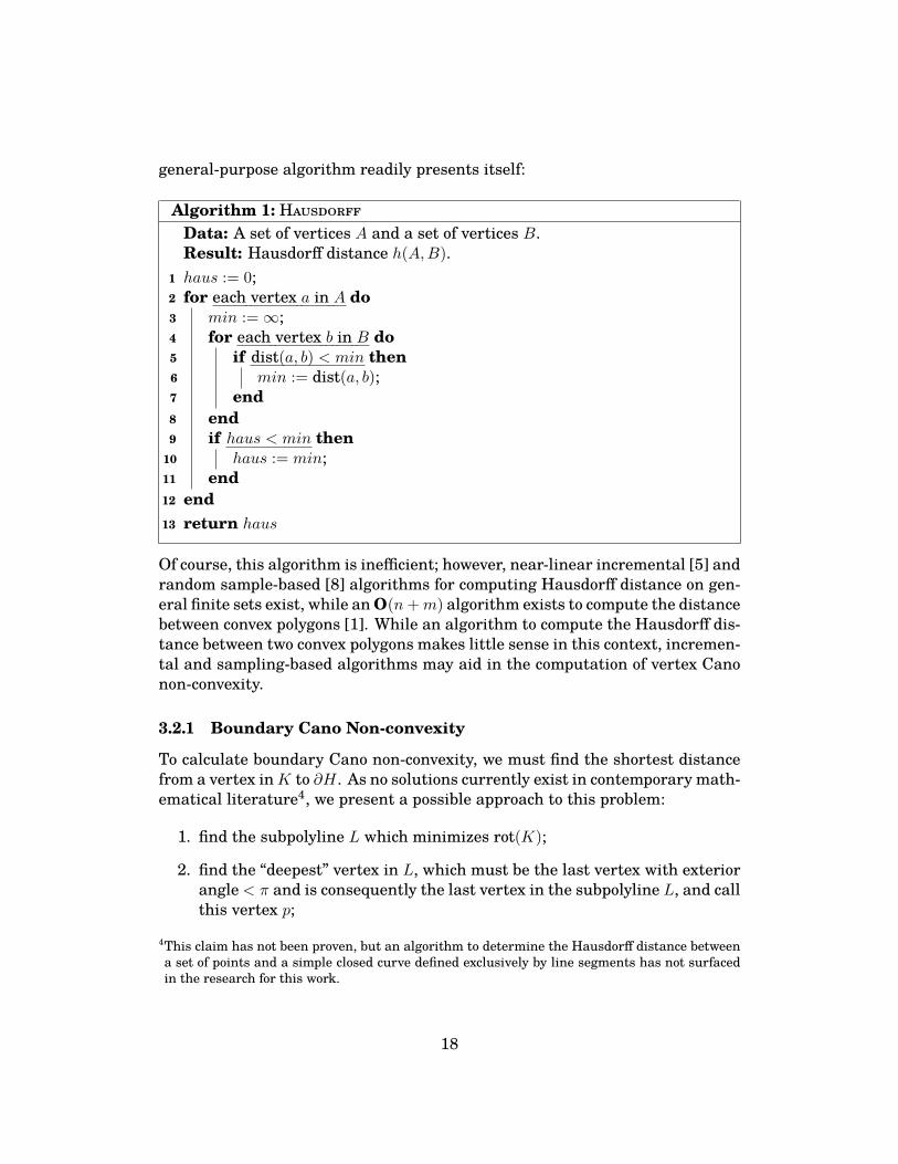
A polygonK (red) with its convex hullH(black). The “worst” vertex and the seg-ment between it and the nearest vertexin the hull is denoted by the blue dashedline.

The same polygon K with its convexhull H. In this diagram, we show thedifference between vertex Cano (as inthe above diagram) and boundary Cano(top-right dashed line).

Similarly to angular non-convexity,Cano non-convexity attempts to cap-ture the “worst” part of a poly-gon; with this measure, though, the“worst” part of the polygon is thevertex vi such that the shortest dis-tance between itself and the near-est vertex on the hull hi is thelargest over all shortest distances.However, this implementation has asignificant shortcoming when poly-gons and hulls are defined exclu-sively by their vertices: if we defineK and H exclusively by an order-ing on their vertices, then Cano non-convexity finds only theHausdorff dis-tance from the vertices of K to thevertices of H, not to the boundary ofH.

We can delineate these two interpre-tations: we refer to the Hausdorff dis-tance betweenK ’s andH ’s vertices asvertex Cano non-convexity, whilewe refer to the Hausdorff distancefromK ’s vertices to ∂H as boundaryCano non-convexity. Intuitively,vertex Cano non-convexity describesthe maximum distance a vertex mustbe pulled to lie on top of a vertex onthe hull, while boundary Cano non-

convexity finds the depth of the largest divot in the polygon.

Vertex Cano non-convexity is easier to compute, in the sense that a naïveO(|K| · |H|)

17

general-purpose algorithm readily presents itself:

Algorithm 1: HausdorffData: A set of vertices A and a set of vertices B.Result: Hausdorff distance h(A,B).

1 haus := 0;2 for each vertex a in A do3 min :=∞;4 for each vertex b in B do5 if dist(a, b) < min then6 min := dist(a, b);7 end8 end9 if haus < min then

10 haus := min;11 end12 end13 return haus

Of course, this algorithm is inefficient; however, near-linear incremental [5] andrandom sample-based [8] algorithms for computing Hausdorff distance on gen-eral finite sets exist, while anO(n+m) algorithm exists to compute the distancebetween convex polygons [1]. While an algorithm to compute the Hausdorff dis-tance between two convex polygons makes little sense in this context, incremen-tal and sampling-based algorithms may aid in the computation of vertex Canonon-convexity.

3.2.1 Boundary Cano Non-convexity

To calculate boundary Cano non-convexity, we must find the shortest distancefrom a vertex inK to ∂H. As no solutions currently exist in contemporary math-ematical literature4, we present a possible approach to this problem:

1. find the subpolyline L which minimizes rot(K);

2. find the “deepest” vertex in L, which must be the last vertex with exteriorangle< π and is consequently the last vertex in the subpolyline L, and callthis vertex p;

4This claim has not been proven, but an algorithm to determine the Hausdorff distance betweena set of points and a simple closed curve defined exclusively by line segments has not surfacedin the research for this work.

18

3. determine the last vertex b on the convex hull which precedes p in theordering;

4. determine the first vertex a on the convex hull which succeeds p in theordering;

5. the distance h(K, ∂H) is the height of the triangle 4bpa.

We have already given a linear-time algorithm to find theminimum circular con-tiguous subarray sum in Section 3.1.2 a simple alteration to store the vertices inthe minimizing subpolyline does not change the running time of the algorithm,so (1) takes time linear in the number of vertices in K, and (2) takes constanttime. Secondly, both (3) and (4) take linear time, as we only need to walk alongthe vertices starting at p in the counter-clockwise direction to find a, and in theclockwise direction to find b. Finally, (5) can be calculated in constant time.Thus, our algorithm can compute the boundary Cano non-convexity in overalllinear time.

Both variations on Cano non-convexity are useful – even though they may en-code different information – and can be easily computed. For this reason, Canonon-convexity appears to be a reasonable alternative to traditional compactnessscores. Furthermore, as boundary Cano non-convexity does an adequate job ofcapturing shape and is not area-comparative, it serves as a more approachableand consistent version of the Reock score.

4 ConclusionsTraditional compactness scores, as they stand, have serious consistency andgameability issues: while they should not be done away with, no single scoreshould be used to determine whether a district is compact or not, especiallywhen there are legal consequences to such a decision. We have also clearlydemonstrated that more complex but better-defined measures of non-convexity(and their translations to measures of compactness) can serve as good alterna-tives to these traditional scores. Furthermore, these alternative compactnessmeasures are efficient to implement, and require only basic linear algebra, ge-ometry, and simple programming solutions. As we further our work in the ger-rymandering space, it is important to continually critique and unpack existingmethods, as well as develop new ones: we believe that the presented alternativemethods of measuring non-convexity – and thus, compactness – are meaningfulcontributions to the studies of geometry and gerrymandering.

19

References[1] M.J. Atallah. A Linear Time Algorithm for the Hausdorff Distance Between

Convex Polygons. Purdue University Department of Computer ScienceTechnical Reports, 1983.

[2] J. Cano. A Measure of Non-convexity and Another Extension of Schauder’sTheorem. Bulletin mathematique de la Societe des Sciences Mathematiquesde Roumanie, 34:3–6, 1990.

[3] M. de Berg, M. van Kreveld, M. Overmars, and O. Schwarzkopf.Computational Geometry. Springer, 2000.

[4] R.N. Karasev. A Measure of Non-convexity in the Plane and the MinkowskiSum. Discrete and Computational Geometry, pages 608–621, 2010.

[5] S. Nutanong, E. H. Jacox, and H. Samet. An Incremental HausdorffDistance Calculation Algorithm. Proceedings of the VLDB Endowment,4(8):506–517, 2011.

[6] Daniel D. Polsby and Robert D. Popper. The Third Criterion: Compactnessas a Procedural Safeguard Against Partisan Gerrymandering. Yale Law &Policy Review, 1991.

[7] Ernest C. Reock. A Note: Measuring Compactness as a Requirement forLegislative Apportionment. Midwest Journal of Political Science, 5(1):70–74, 1961.

[8] A.A. Taha and A. Hanbury. An Efficient Algorithm for Calculating the ExactHausdorff Distance. IEEE Transactions on Pattern Analysis and MachineIntelligence, 37(11):2153–2163, 2015.

20