1

Finding the best process setup for one response is hard enough, but what can you do

when faced with customer demands for multiple specifications? Do you ever get

between a rock and a hard place in trying to satisfy all the demands?

If so, we’ve got an approach that may solve all your problems.

* Propagation of error (POE) is also known by several other names; e.g.,

transmitted variance, transmission of error, transmission of variance (TOV),

etc.

©2009 St

at-Eas

e, Inc.

2

©2009 St

at-Eas

e, Inc.

3

Only statistical masochists would do RSM by hand. At the very least, you would use

a regression package to do the fitting. Even this requires tedious coding and careful

interpretation of the output. Better yet, use software specifically geared to RSM. We

will use DESIGN-EXPERT on an example problem. This case study takes you

through the typical steps used in a RSM design. Concentrate on mechanics, do not

get hung-up on analysis details.©2009 St

at-Eas

e, Inc.

4

Only statistical masochists would do RSM by hand. At the very least, you would use

a regression package to do the fitting. Even this requires tedious coding and careful

interpretation of the output. Better yet, use software specifically geared to RSM. We

will use DESIGN-EXPERT on an example problem. This case study takes you

through the typical steps used in a RSM design. Concentrate on mechanics, do not

get hung-up on analysis details.©2009 St

at-Eas

e, Inc.

5

This is a very powerful tool for finding your sweet spot – where all specifications can

be met. But the reliability of the results depends on the validity of your predictive

models.

Each response may have a different model, or a different subset of factors.

©2009 St

at-Eas

e, Inc.

6

A significant model F-value gives you confidence that you can explain what causes

variation. However, some statisticians advise that for prediction purposes, you need

a stronger fit, perhaps as much as 4 times the F value you’d normally accept as

significant. A more straight-forward statistic for determining the strength of your

model for prediction is the adequate precision, which was defined mathematically in

Section 2 in the explanation of outputs from the RSM tutorial. Recall that this

statistic measures the signal by taking the range of predicted response (max to min of

y) which you can read off the case statistic table in the ANOVA report. It ratios this

signal to noise defined by a function of the Mean Square Error (MSE) which comes

from the ANOVA table.

©2009 St

at-Eas

e, Inc.

7

Compare these results to the criteria for good models.

©2009 St

at-Eas

e, Inc.

8

Compare these results to the criteria for good models.

©2009 St

at-Eas

e, Inc.

9

Don't get stalled on new plots or statistics. Focus on learning how to use the

software.

©2009 St

at-Eas

e, Inc.

10

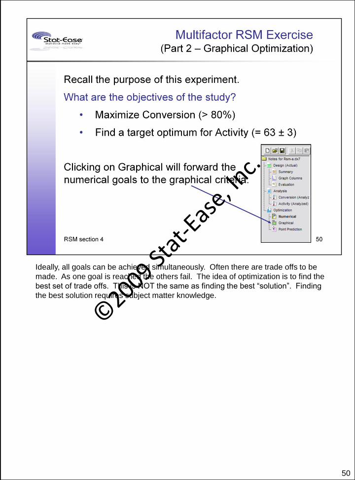
Ideally, all goals can be achieved simultaneously. Often there are trade offs to be

made. As one goal is reached the others fail. The idea of optimization is to find the

best set of trade offs. This is NOT the same as finding the best “solution”. Finding

the best solution requires subject matter knowledge.

©2009 St

at-Eas

e, Inc.

11

Stretching a goal beyond the best observed response allows the optimization

algorithm to look for “better than observed” prediction regions. Once an optimal goal

is reached or exceeded the algorithm no longer attempts to improve that criteria. Be

realistic when stretching. Don’t push the limits too far.

In this case 100% conversion is an obvious natural limit. We could set a practical

upper limit of 97%. If so, then 100% is considered no better than 97%.©2009 St

at-Eas

e, Inc.

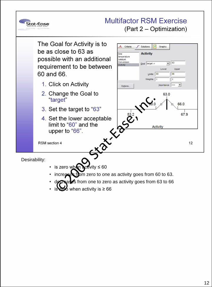
12

Desirability:

• is zero when activity ≤ 60

• increases from zero to one as activity goes from 60 to 63.

• decreases from one to zero as activity goes from 63 to 66

• is zero when activity is ≥ 66©2009 St

at-Eas

e, Inc.

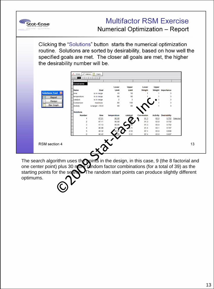
13

The search algorithm uses the points in the design, in this case, 9 (the 8 factorial and

one center point) plus 30 more random factor combinations (for a total of 39) as the

starting points for the search. The random start points can produce slightly different

optimums.

©2009 St

at-Eas

e, Inc.

14

Use the Ramps view to compare the solutions; clicking on the solution numbers one

after another and see what changes on the ramps.

©2009 St

at-Eas

e, Inc.

15

©2009 St

at-Eas

e, Inc.

16

It’s very common that experimenters must contend with multiple responses. In such

cases it helps to use a numerical approach that entails construction of an objective

function "big D", which represents desirable combinations. This turns out to be a

handy way to make tradeoffs between multiple responses that’s very simple.

You will find this to be a common-sense approach that can be easily explained to

your colleagues. It offers advantages over the main alternative, linear programming,

which assumes that you want to optimize one major response subject to constraints

on the remaining responses. Desirability functions allow balancing of all responses

with the additional advantage that the result can be plotted.

The function involves assignment of desirabilities to each response. Use of

geometric mean to calculate overall desirability provides the property that if any one

response attains zero desirability then the overall desirability will be zero. It's all or

nothing.

For further details see G. C. Derringer, “A Balancing Act: Optimizing a Product’s

Properties.” Quality Progress, June 1994 in the appendix of this manual and posted

on our web site at http://www.statease.com/pubs/derringer.pdf.

©2009 St

at-Eas

e, Inc.

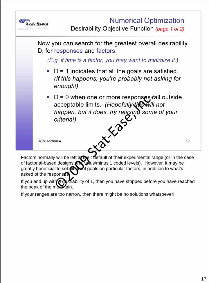
17

Factors normally will be left at their default of their experimental range (or in the case

of factorial-based designs, their plus/minus 1 coded levels). However, it may be

greatly beneficial to set different goals on particular factors, in addition to what’s

asked of the responses.

If you end up with a desirability of 1, then you have stopped before you have reached

the peak of the mountain.

If your ranges are too narrow, then there might be no solutions whatsoever!©

2009 Stat

-Ease, In

c.

18

The assignment of optimization parameters is where your subject matter expertise

and knowledge of customer requirements becomes the key to getting a good

outcome.

The goal and limits define the “d’s”

©2009 St

at-Eas

e, Inc.

19

It is best to start by keeping things as simple as possible. Then after seeing what

happens, impose further parameters such as the weight and/or importance on

specific responses (or factors – do not forget that these can also be manipulated in

the optimization).

©2009 St

at-Eas

e, Inc.

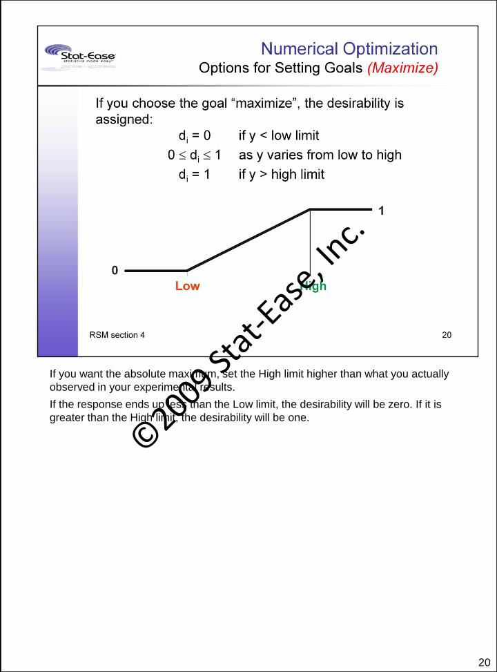
20

If you want the absolute maximum, set the High limit higher than what you actually

observed in your experimental results.

If the response ends up less than the Low limit, the desirability will be zero. If it is

greater than the High limit, the desirability will be one.

©2009 St

at-Eas

e, Inc.

21

To get the absolute maximum, set the upper limit to its theoretical limit of 100%.

©2009 St

at-Eas

e, Inc.

22

This goal is the one you will use for the typical product specification. Try to negotiate

the widest range possible!

©2009 St

at-Eas

e, Inc.

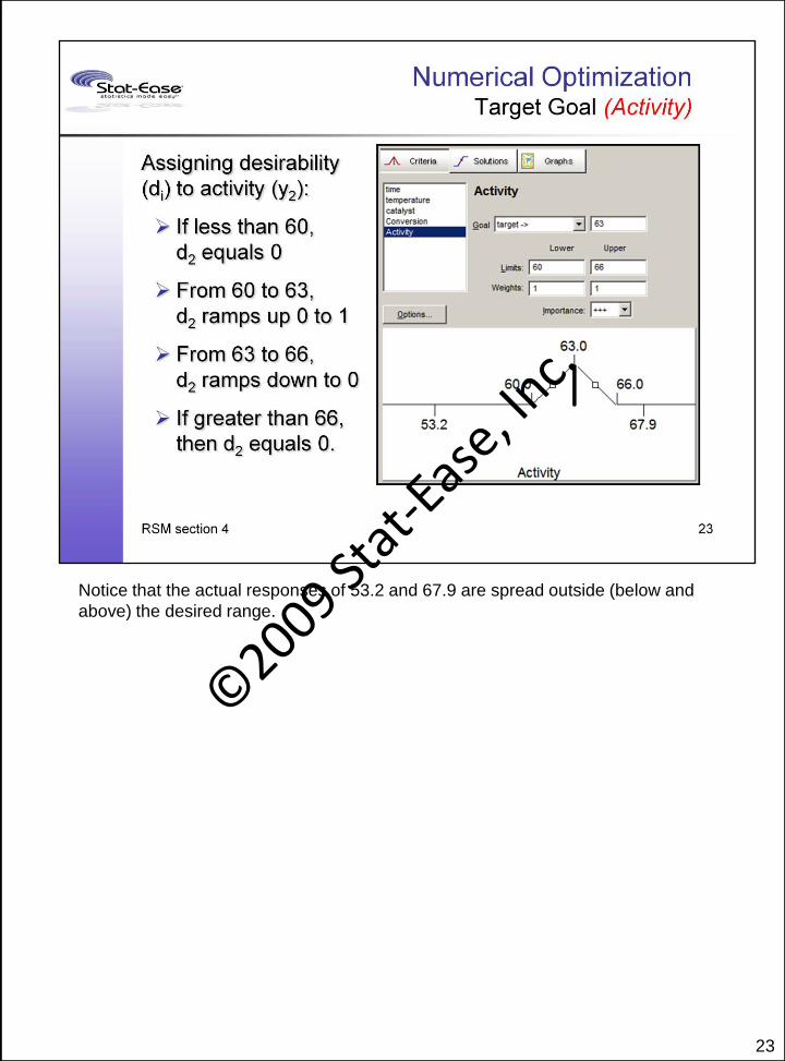
23

Notice that the actual responses of 53.2 and 67.9 are spread outside (below and

above) the desired range.

©2009 St

at-Eas

e, Inc.

24

If you want the absolute minimum, set the low limit very low – below what you

actually observed in your experimental results.

©2009 St

at-Eas

e, Inc.

25

Design-Expert will set the limits at the plus/minus 1 (coded) range for CCD’s, even if

their alpha values exceed 1 and thus put actual values further out. The idea for

CCD’s is to “stay inside the box” when making predictions and seeking optimum

values. Users, if they dare, may push these limits out, hopefully only to take a stab in

the dark.

Technical note: Per Derringer and Suich, the goal of range is considered to be simply

a constraint, so the di , although they get included in the product of the desirability

function "D", are not counted in determining "n" for D=(πdi)1/n.

©2009 St

at-Eas

e, Inc.

26

Technical note: The individual desirability generated from the equality goal is not

included in the product for computation of the overall desirability.

Why can’t you set a response to “is equal to?” Answer: You don’t have direct control

of the response – there is no knob to dial it in. Instead, the response is a function of

the factors you can control.©2009 St

at-Eas

e, Inc.

27

Nobody is forcing you to optimize any particular response! For instance, if a particular

response did not result in a good prediction model, then it may be better to leave it

out of the optimization. Remember, “garbage in will send garbage out.”

©2009 St

at-Eas

e, Inc.

28

If you want to really fine-tune the optimization, you can assign weights. These affect

the shapes of the ramps so they more closely approximate what your customers

want.

Weights greater than 1 give more emphasis to the goal.

Weights less than 1 give less emphasis to the goal.©2009 St

at-Eas

e, Inc.

29

Let’s see how weights affect maximization. Higher weights put more emphasis on the

goal. For example if we began with an un-weighted desirability of 0.5, what would

happen with a weight of 2? (Answer: desirability drops to 0.25. Therefore the

program will not be satisfied until it pushes closer to the high threshold on this

response.) What happens with a weight of 0.5? (Answer: desirability increases to

about 0.7. Therefore the program will be satisfied fairly quickly once it reaches the

low threshold.) ©2009 St

at-Eas

e, Inc.

30

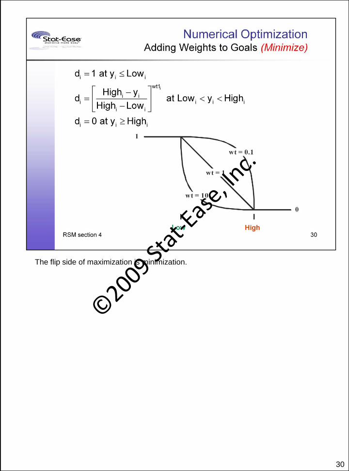
The flip side of maximization is minimization.

©2009 St

at-Eas

e, Inc.

31

To get really fancy you can use weights on a goal as target and shape to your liking,

or better yet, your customer’s. You could even approximate the Taguchi quadratic

loss function, which being negative is U-shaped so you’d want desirability, a positive

attribute, to be an upside-down “U” – done by setting weights below 1 on either side,

for example at the minimum value of 0.1.

©2009 St

at-Eas

e, Inc.

32

There are no weights associated goals of “in range” and “equal to”. These goals that

have only zero or one as possible values and weights would have no effect.

©2009 St

at-Eas

e, Inc.

33

If you’re concerned more about setting priorities to your responses (and you usually

are), use this feature.

Note that if all importance ratings are the same, then they have no impact.

©2009 St

at-Eas

e, Inc.

34

The assignment of optimization parameters is where your subject matter expertise is

incorporated into the search for the optimum formula.

©2009 St

at-Eas

e, Inc.

35

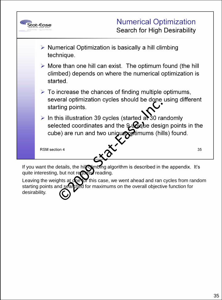
If you want the details, the hill-climbing algorithm is described in the appendix. It’s

quite interesting, but not required reading.

Leaving the weights at one for this case, we went ahead and ran cycles from random

starting points and searched for maximums on the overall objective function for

desirability. ©2009 St

at-Eas

e, Inc.

36

Since it's not easy to anticipate what will happen with weighting, we advise that you

begin with weights of 1. You might also go with wider windows to be sure that some

desirable regions will be opened. Then narrow down the windows and add weights

and importance ratings if needed.

Leaving the weights at one for this case, we went ahead and ran 30 cycles from

random starting points and searched for maximums on the univariate objective

function for desirability. Two separate hills were found. Other solutions are

duplicates that passed through the filter in Design-Expert software. You can adjust

the filter via the Options button on the Criteria screen for Numerical Optimization.

The scale for the filter slide bar is labeled “Epsilon.” Moving epsilon up causes fewer

solutions to be reported and vice-versa.

©2009 St

at-Eas

e, Inc.

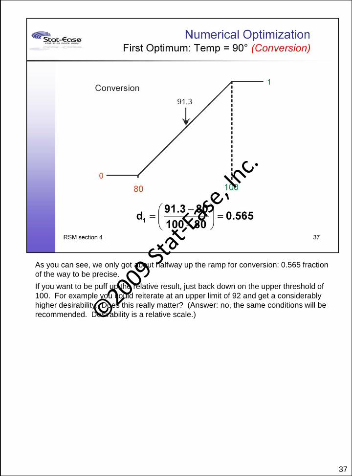
37

As you can see, we only got about halfway up the ramp for conversion: 0.565 fraction

of the way to be precise.

If you want to be puff up the relative result, just back down on the upper threshold of

100. For example you could reiterate at an upper limit of 92 and get a considerably

higher desirability. Does this really matter? (Answer: no, the same conditions will be

recommended. Desirability is a relative scale.)©2009 St

at-Eas

e, Inc.

38

This optimum hits the activity target. The overall desirability then becomes the

square root of the product of the two individual desirabilities.

©2009 St

at-Eas

e, Inc.

39

The higher of the two optimums is at 90 degrees.

©2009 St

at-Eas

e, Inc.

40

The lower of the two optimums is at 80 degrees.

©2009 St

at-Eas

e, Inc.

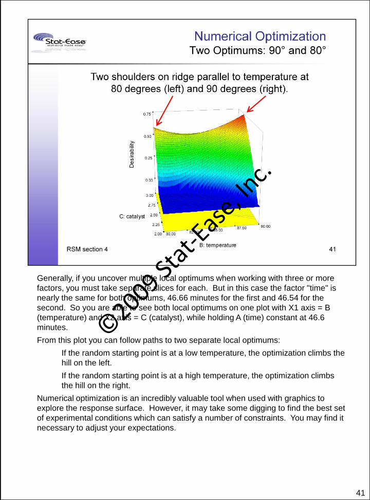
41

Generally, if you uncover multiple local optimums when working with three or more

factors, you must take separate slices for each. But in this case the factor "time" is

nearly the same for both optimums, 46.66 minutes for the first and 46.54 for the

second. So you are able to see both local optimums on one plot with X1 axis = B

(temperature) and X2 axis = C (catalyst), while holding A (time) constant at 46.6

minutes.

From this plot you can follow paths to two separate local optimums:

If the random starting point is at a low temperature, the optimization climbs the

hill on the left.

If the random starting point is at a high temperature, the optimization climbs

the hill on the right.

Numerical optimization is an incredibly valuable tool when used with graphics to

explore the response surface. However, it may take some digging to find the best set

of experimental conditions which can satisfy a number of constraints. You may find it

necessary to adjust your expectations.

©2009 St

at-Eas

e, Inc.

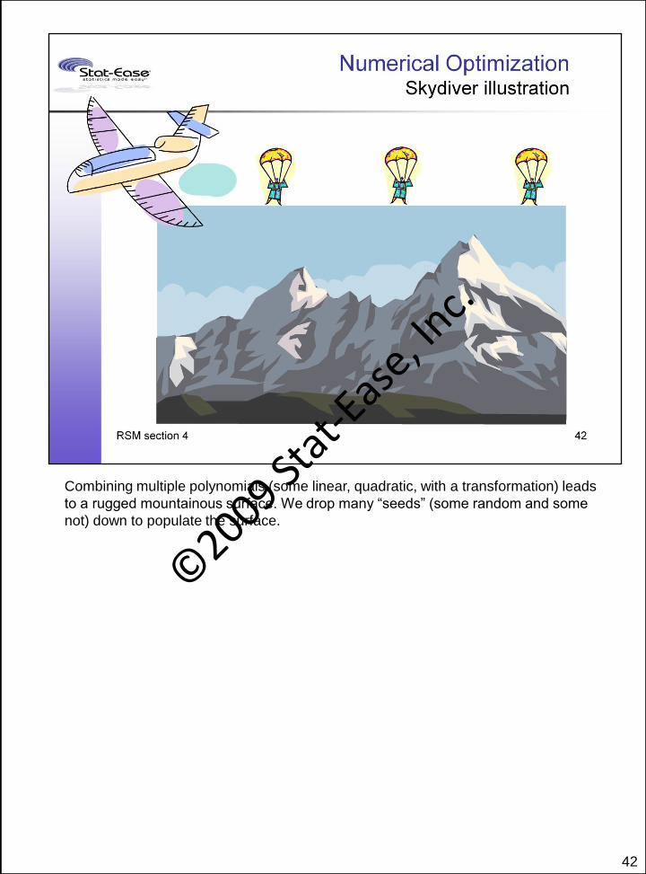
Combining multiple polynomials (some linear, quadratic, with a transformation) leads

to a rugged mountainous surface. We drop many “seeds” (some random and some

not) down to populate the surface.

42

©2009 St

at-Eas

e, Inc.

When the “seeds” or skydivers land, they are instructed to walk “up” (increasing

desirability) until they can’t find a higher point.

Notice that:

• Multiple peaks can be found.

• If several seeds land on the same mountain, they will converge to a single peak.

• Plateaus will lead to many more “solutions” because there is no way to go up.

• The step size will influence finding the exact peak.

43

©2009 St

at-Eas

e, Inc.

44

A simplex is a geometric figure having a number of vertexes equal to one more than

the number of independent factors. For two factor, the simplex forms an equilateral

triangle as shown here. It's been found that simplex optimization as outlined here is a

relatively efficient approach that's very robust to case variations. It requires only

function evaluations, not derivatives.

After randomly choosing a starting point, we move toward the center of the

experimental space to form the simplex. You can choose the size, which the program

defaults to 10%.

Further details:

The use of next to worst ("n") from previous simplex ensures that won't get stuck in

flip-flop (like rubber raft stuck in "hydraulic" trough). The last "N" becomes the new

"W" which might better be termed "wastebasket" because it may not be worst.

What will happen if all points are on the zero desirability plane? (Answer: you're

stuck! DESIGN-EXPERT will move toward measurable levels by a proprietary

method.)

©2009 St

at-Eas

e, Inc.

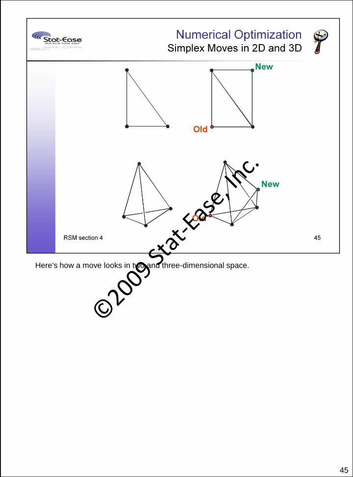
45

Here's how a move looks in two and three-dimensional space.

©2009 St

at-Eas

e, Inc.

46

We drew up an example that shows how the simplex climbs the hill. Note that at the

end it begins overlap itself in a spin. This phenomenon is unique to one and two

dimensions. Three dimensional tetrahedral and higher dimensional hyper-tetrahedra

do not close pack so they will not overlap. As soon as you see overlap, the

optimization should be terminated.

The simplexes we've looked at so far are fixed size. Next we look at a more effective

strategy which entails use of variable size simplexes.©

2009 Stat

-Ease, In

c.

47

In 1965, Nelder and Mead made modifications to the simplex algorithm which allow

expansion in favorable directions and contractions in unfavorable directions.

Reducing this simple concept to hard rules of logic makes it look more complicated

than it needs to be. Once you get it figured out it becomes very mechanical.

Reminder: B is the best point, W is the worst point and N is the next to worst point.

You can see from the pictures that the expansion point doubles the fixed step from

the centroid of the hyperface. The contraction draws in the step by 50 percent.

If the reflection point falls between the previous best and next worst, B and N, then

we stay there. Some practitioners call this the "Ho Hum" vertex because it's so

mediocre.

©2009 St

at-Eas

e, Inc.

48

In 1965, Nelder and Mead made modifications to the simplex algorithm which allow

expansion in favorable directions and contractions in unfavorable directions. They

reduced this simple concept to just a handful of hard rules of logic that work well

programatically.

As you can see, the variable simplex feeds on gradients. Like a living organism, it

grows up hills and shrinks around the peaks. It’s kind of a wild thing, but little harm

can occur as long as it stays caged in the computer. The animated GIF (copied from

http://www.chem.uoa.gr/Applets/appletsimplex/Text_Simplex2.htm) shows for a single

simplex the various moves – contraction versus expansion.

On the other hand, the fixed size simplex shown earlier plods robotically in

appropriate vectors and then cartwheels around the peak. This is a more

conservative procedure if done on a real process, but since no harm can be done

using it with RSM models, it’s better to use the variable-sized simplex for more

precise results in a similar number of moves.

©2009 St

at-Eas

e, Inc.

49

©2009 St

at-Eas

e, Inc.

50

Ideally, all goals can be achieved simultaneously. Often there are trade offs to be

made. As one goal is reached the others fail. The idea of optimization is to find the

best set of trade offs. This is NOT the same as finding the best “solution”. Finding

the best solution requires subject matter knowledge.

©2009 St

at-Eas

e, Inc.

51

Here's the plot of time and catalyst with temperature sliced at 90.

Notice that since you want to maximize Conversion, it only has a lower bound and not

an upper bound.

Activity will have both a lower and an upper bound since it is trying to achieve a target

value. ©2009 St

at-Eas

e, Inc.

52

Here's the plot of time and catalyst with temperature changed to be sliced at 80.

©2009 St

at-Eas

e, Inc.

53

The graphical optimization will be more presentable to your clients because it shows

the “sweet spots” where all specifications can be met. If this operating window is too

small, click on each border to identify specifications that perhaps could be relaxed.

Conversely, if specifications have been applied loosely, some might be tightened up

with no effect on the “sweet spot” because they don’t form it’s borders.

The “Optimization Guide” starts on page 2-14 of the Handbook.©2009 St

at-Eas

e, Inc.

54

©2009 St

at-Eas

e, Inc.