Embed Size (px)
Citation preview
Stable Complete Intersections
M. TorrenteUniversity of Genova
(joint work with L. Robbiano)
MEGA 2011, Stockholm
M. Torrente (University of Genova) Stable Complete Intersections MEGA 2011 1 / 22
Introduction
Introduction
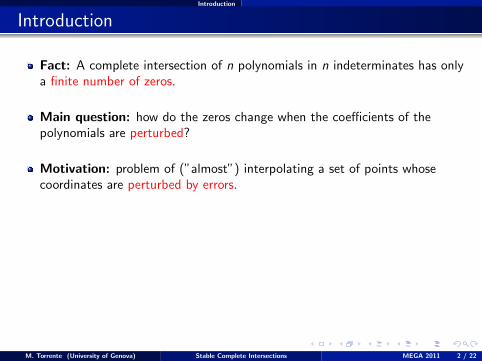
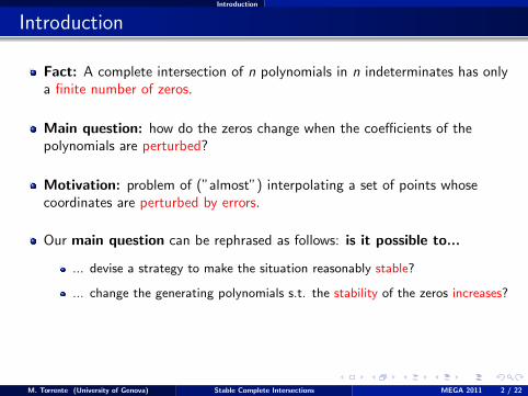
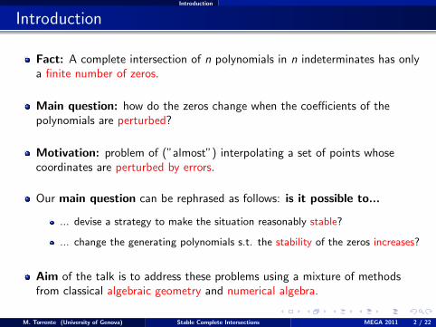
Fact: A complete intersection of n polynomials in n indeterminates has onlya finite number of zeros.
Main question: how do the zeros change when the coefficients of thepolynomials are perturbed?
Motivation: problem of (”almost”) interpolating a set of points whosecoordinates are perturbed by errors.
Our main question can be rephrased as follows: is it possible to...
... devise a strategy to make the situation reasonably stable?
... change the generating polynomials s.t. the stability of the zeros increases?
Aim of the talk is to address these problems using a mixture of methodsfrom classical algebraic geometry and numerical algebra.
M. Torrente (University of Genova) Stable Complete Intersections MEGA 2011 2 / 22
Introduction
Introduction
Fact: A complete intersection of n polynomials in n indeterminates has onlya finite number of zeros.
Main question: how do the zeros change when the coefficients of thepolynomials are perturbed?
Motivation: problem of (”almost”) interpolating a set of points whosecoordinates are perturbed by errors.
Our main question can be rephrased as follows: is it possible to...
... devise a strategy to make the situation reasonably stable?
... change the generating polynomials s.t. the stability of the zeros increases?
Aim of the talk is to address these problems using a mixture of methodsfrom classical algebraic geometry and numerical algebra.
M. Torrente (University of Genova) Stable Complete Intersections MEGA 2011 2 / 22
Introduction
Motivating example - The Linear Case
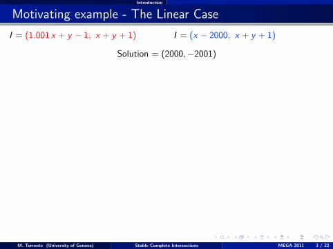
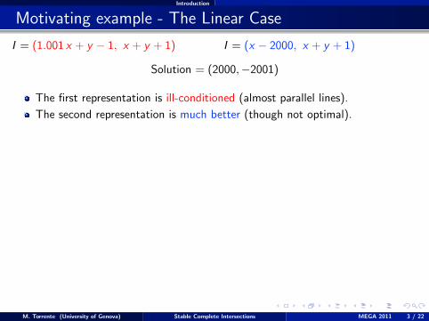
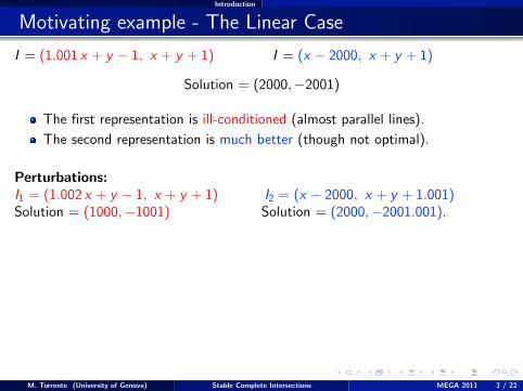
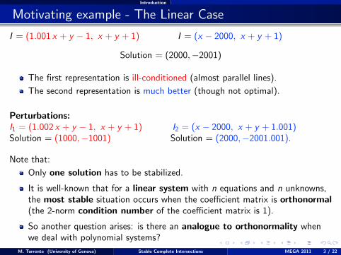
I = (1.001 x + y − 1, x + y + 1) I = (x − 2000, x + y + 1)
Solution = (2000,−2001)
The first representation is ill-conditioned (almost parallel lines).
The second representation is much better (though not optimal).
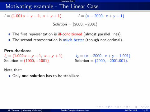
Perturbations:I1 = (1.002 x + y − 1, x + y + 1) I2 = (x − 2000, x + y + 1.001)Solution = (1000,−1001) Solution = (2000,−2001.001).
Note that:
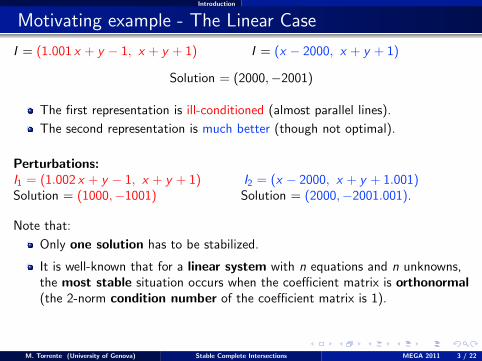
Only one solution has to be stabilized.
It is well-known that for a linear system with n equations and n unknowns,the most stable situation occurs when the coefficient matrix is orthonormal(the 2-norm condition number of the coefficient matrix is 1).
So another question arises: is there an analogue to orthonormality whenwe deal with polynomial systems?
M. Torrente (University of Genova) Stable Complete Intersections MEGA 2011 3 / 22
Introduction
Motivating example - The Linear Case
I = (1.001 x + y − 1, x + y + 1) I = (x − 2000, x + y + 1)
Solution = (2000,−2001)
The first representation is ill-conditioned (almost parallel lines).
The second representation is much better (though not optimal).
Perturbations:I1 = (1.002 x + y − 1, x + y + 1) I2 = (x − 2000, x + y + 1.001)Solution = (1000,−1001) Solution = (2000,−2001.001).
Note that:
Only one solution has to be stabilized.
It is well-known that for a linear system with n equations and n unknowns,the most stable situation occurs when the coefficient matrix is orthonormal(the 2-norm condition number of the coefficient matrix is 1).
So another question arises: is there an analogue to orthonormality whenwe deal with polynomial systems?
M. Torrente (University of Genova) Stable Complete Intersections MEGA 2011 3 / 22

Introduction
Plan of the talk
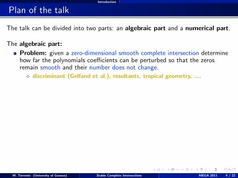
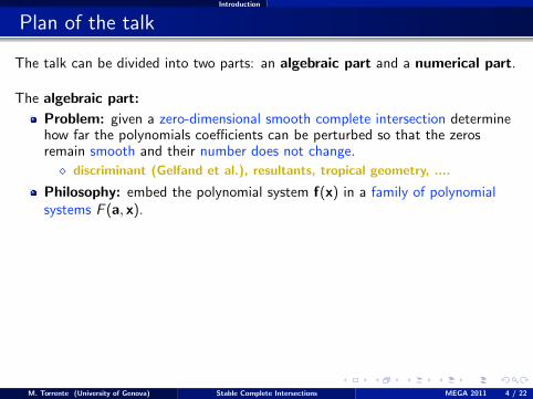
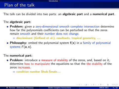
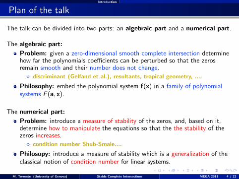
The talk can be divided into two parts: an algebraic part and a numerical part.
The algebraic part:
Problem: given a zero-dimensional smooth complete intersection determinehow far the polynomials coefficients can be perturbed so that the zerosremain smooth and their number does not change.
� discriminant (Gelfand et al.), resultants, tropical geometry, ....
Philosophy: embed the polynomial system f(x) in a family of polynomialsystems F (a, x).
The numerical part:
Problem: introduce a measure of stability of the zeros, and, based on it,determine how to manipulate the equations so that the the stability of thezeros increases.
� condition number Shub-Smale....
Philosopy: introduce a measure of stability which is a generalization of theclassical notion of condition number for linear systems.
M. Torrente (University of Genova) Stable Complete Intersections MEGA 2011 4 / 22
Introduction
Plan of the talk
The talk can be divided into two parts: an algebraic part and a numerical part.
The algebraic part:
Problem: given a zero-dimensional smooth complete intersection determinehow far the polynomials coefficients can be perturbed so that the zerosremain smooth and their number does not change.
� discriminant (Gelfand et al.), resultants, tropical geometry, ....
Philosophy: embed the polynomial system f(x) in a family of polynomialsystems F (a, x).
The numerical part:
Problem: introduce a measure of stability of the zeros, and, based on it,determine how to manipulate the equations so that the the stability of thezeros increases.
� condition number Shub-Smale....
Philosopy: introduce a measure of stability which is a generalization of theclassical notion of condition number for linear systems.
M. Torrente (University of Genova) Stable Complete Intersections MEGA 2011 4 / 22
The algebraic part
Notations
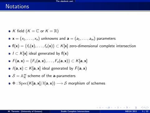
K field (K = C or K = R)
x = (x1, . . . , xn) unknowns and a = (a1, . . . , am) parameters
f(x) = {f1(x), . . . , fn(x)} ⊂ K [x] zero-dimensional complete intersection
I ⊂ K [x] ideal generated by f(x)
F (a, x) = {F1(a, x), . . . ,Fn(a, x)} ⊂ K [a, x]
I (a, x) ⊂ K [a, x] ideal generated by F (a, x)
S = AmK scheme of the a-parameters
Φ : Spec(K [a, x]/I (a, x)) −→ S morphism of schemes
M. Torrente (University of Genova) Stable Complete Intersections MEGA 2011 5 / 22
The algebraic part
Freeness
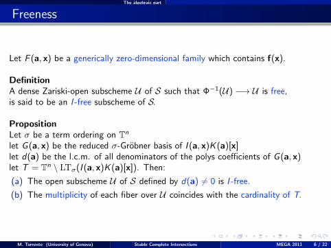
Let F (a, x) be a generically zero-dimensional family which contains f(x).
DefinitionA dense Zariski-open subscheme U of S such that Φ−1(U) −→ U is free,is said to be an I -free subscheme of S.
PropositionLet σ be a term ordering on Tn
let G (a, x) be the reduced σ-Grobner basis of I (a, x)K (a)[x]let d(a) be the l.c.m. of all denominators of the polys coefficients of G (a, x)let T = Tn \ LTσ(I (a, x)K (a)[x]). Then:
(a) The open subscheme U of S defined by d(a) 6= 0 is I -free.
(b) The multiplicity of each fiber over U coincides with the cardinality of T.
M. Torrente (University of Genova) Stable Complete Intersections MEGA 2011 6 / 22
The algebraic part
Freeness
Let F (a, x) be a generically zero-dimensional family which contains f(x).
DefinitionA dense Zariski-open subscheme U of S such that Φ−1(U) −→ U is free,is said to be an I -free subscheme of S.
PropositionLet σ be a term ordering on Tn
let G (a, x) be the reduced σ-Grobner basis of I (a, x)K (a)[x]let d(a) be the l.c.m. of all denominators of the polys coefficients of G (a, x)let T = Tn \ LTσ(I (a, x)K (a)[x]). Then:
(a) The open subscheme U of S defined by d(a) 6= 0 is I -free.
(b) The multiplicity of each fiber over U coincides with the cardinality of T.
M. Torrente (University of Genova) Stable Complete Intersections MEGA 2011 6 / 22
The algebraic part
Smoothness
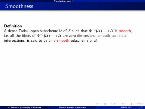
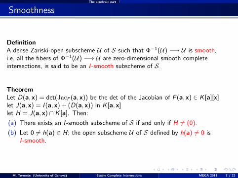
DefinitionA dense Zariski-open subscheme U of S such that Φ−1(U) −→ U is smooth,i.e. all the fibers of Φ−1(U) −→ U are zero-dimensional smooth completeintersections, is said to be an I -smooth subscheme of S.
TheoremLet D(a, x) = det(JacF (a, x)) be the det of the Jacobian of F (a, x) ∈ K [a][x]let J(a, x) = I (a, x) + (D(a, x)) in K [a, x]let H = J(a, x) ∩ K [a]. Then:
(a) There exists an I -smooth subscheme of S if and only if H 6= (0).
(b) Let 0 6= h(a) ∈ H; the open subscheme U of S defined by h(a) 6= 0 isI -smooth.
M. Torrente (University of Genova) Stable Complete Intersections MEGA 2011 7 / 22
The algebraic part
Smoothness
DefinitionA dense Zariski-open subscheme U of S such that Φ−1(U) −→ U is smooth,i.e. all the fibers of Φ−1(U) −→ U are zero-dimensional smooth completeintersections, is said to be an I -smooth subscheme of S.
TheoremLet D(a, x) = det(JacF (a, x)) be the det of the Jacobian of F (a, x) ∈ K [a][x]let J(a, x) = I (a, x) + (D(a, x)) in K [a, x]let H = J(a, x) ∩ K [a]. Then:
(a) There exists an I -smooth subscheme of S if and only if H 6= (0).
(b) Let 0 6= h(a) ∈ H; the open subscheme U of S defined by h(a) 6= 0 isI -smooth.
M. Torrente (University of Genova) Stable Complete Intersections MEGA 2011 7 / 22
The algebraic part
Freeness + Smoothness = Optimality
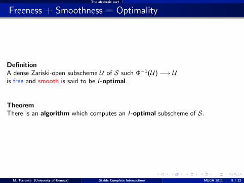
DefinitionA dense Zariski-open subscheme U of S such Φ−1(U) −→ Uis free and smooth is said to be I -optimal.
TheoremThere is an algorithm which computes an I -optimal subscheme of S.
M. Torrente (University of Genova) Stable Complete Intersections MEGA 2011 8 / 22
The algebraic part
An example
We consider the ideal I = (xy + 1, x2 + y2 − 5) ∈ R[x , y ] embedded into thefamily I (a, x , y) = (xy + a1x + 1, x2 + y2 + a2).
Freeness
We compute the reduced Lex-Grobner basis of I (a, x)K (a)[x , y ]
g1 = x − y3 − a1y2 − a2y − a1a2,
g2 = y4 + 2a1y3 + (a21 + a2)y2 + 2a1a2y + (a21a2 + 1)
There is no condition for the free locus.
Smoothness
We compute D(a, x , y) = det(JacF (a, x , y)) = −2x2 + 2y2 + 2a1y ,J(a, x , y) = I (a, x , y) + (D(a, x , y)) and H = J(a, x , y) ∩ K [a] = (h(a))
h(a) = a61a2 + 3a41a22 + a41 + 3a21a
32 + 20a21a2 + a42 − 8a22 + 16
Optimality
An I -optimal subscheme is U = {α ∈ A2R : h(α1, α2) 6= 0}.
M. Torrente (University of Genova) Stable Complete Intersections MEGA 2011 9 / 22
The algebraic part
What about real zeros?
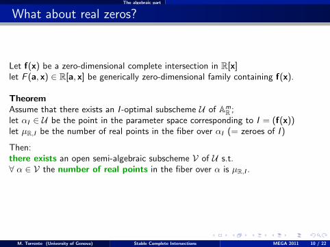
Let f(x) be a zero-dimensional complete intersection in R[x]let F (a, x) ∈ R[a, x] be generically zero-dimensional family containing f(x).
TheoremAssume that there exists an I -optimal subscheme U of Am
R ;let αI ∈ U be the point in the parameter space corresponding to I = (f(x))let µR,I be the number of real points in the fiber over αI (= zeroes of I )
Then:there exists an open semi-algebraic subscheme V of U s.t.∀ α ∈ V the number of real points in the fiber over α is µR,I .
� proof Shape Lemma + theorem Basu-Pollack-Roy
M. Torrente (University of Genova) Stable Complete Intersections MEGA 2011 10 / 22
The algebraic part
What about real zeros?
Let f(x) be a zero-dimensional complete intersection in R[x]let F (a, x) ∈ R[a, x] be generically zero-dimensional family containing f(x).
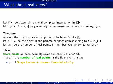
TheoremAssume that there exists an I -optimal subscheme U of Am
R ;let αI ∈ U be the point in the parameter space corresponding to I = (f(x))let µR,I be the number of real points in the fiber over αI (= zeroes of I )
Then:there exists an open semi-algebraic subscheme V of U s.t.∀ α ∈ V the number of real points in the fiber over α is µR,I .
� proof Shape Lemma + theorem Basu-Pollack-Roy
M. Torrente (University of Genova) Stable Complete Intersections MEGA 2011 10 / 22
The algebraic part
An example: continuation 1
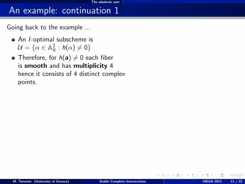
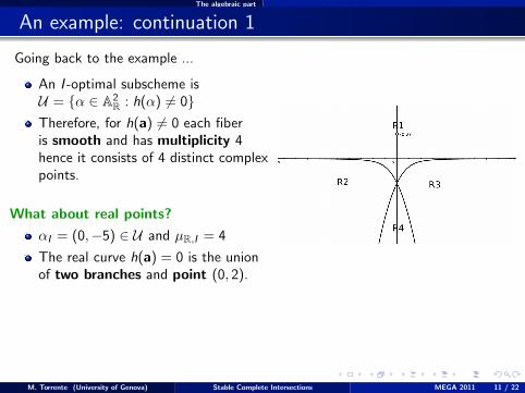
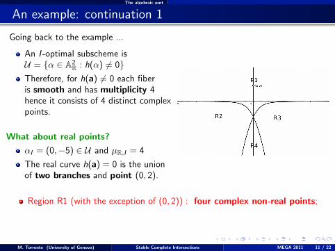
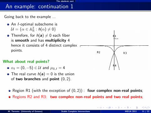
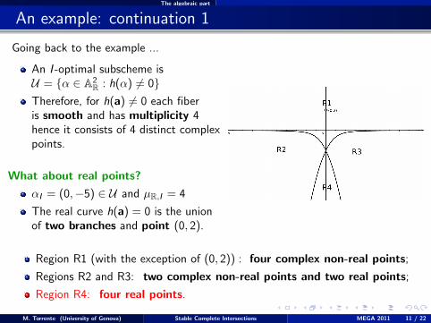
Going back to the example ...
An I -optimal subscheme isU = {α ∈ A2
R : h(α) 6= 0}Therefore, for h(a) 6= 0 each fiberis smooth and has multiplicity 4hence it consists of 4 distinct complexpoints.
What about real points?
αI = (0,−5) ∈ U and µR,I = 4
The real curve h(a) = 0 is the unionof two branches and point (0, 2).
Region R1 (with the exception of (0, 2)) : four complex non-real points;
Regions R2 and R3: two complex non-real points and two real points;
Region R4: four real points.
M. Torrente (University of Genova) Stable Complete Intersections MEGA 2011 11 / 22
The algebraic part
An example: continuation 1
Going back to the example ...
An I -optimal subscheme isU = {α ∈ A2
R : h(α) 6= 0}Therefore, for h(a) 6= 0 each fiberis smooth and has multiplicity 4hence it consists of 4 distinct complexpoints.
What about real points?
αI = (0,−5) ∈ U and µR,I = 4
The real curve h(a) = 0 is the unionof two branches and point (0, 2).
Region R1 (with the exception of (0, 2)) : four complex non-real points;
Regions R2 and R3: two complex non-real points and two real points;
Region R4: four real points.
M. Torrente (University of Genova) Stable Complete Intersections MEGA 2011 11 / 22
The algebraic part
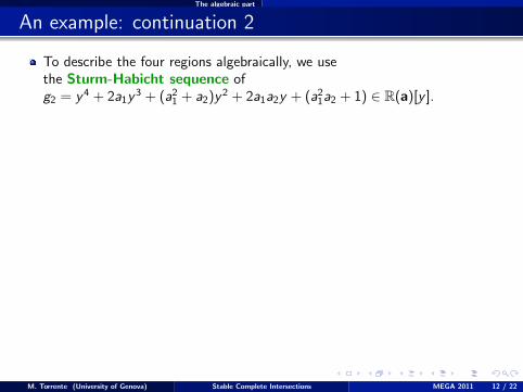
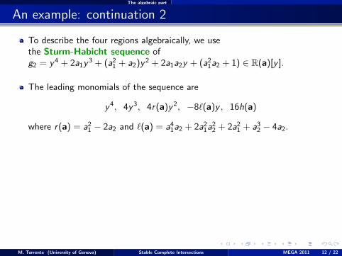
An example: continuation 2
To describe the four regions algebraically, we usethe Sturm-Habicht sequence ofg2 = y4 + 2a1y
3 + (a21 + a2)y2 + 2a1a2y + (a21a2 + 1) ∈ R(a)[y ].
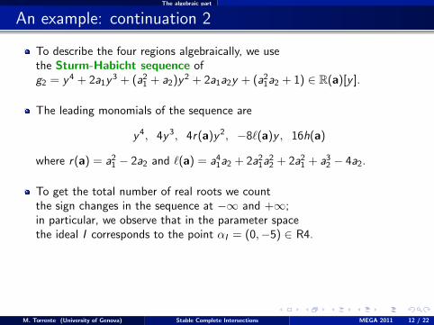
The leading monomials of the sequence are
y4, 4y3, 4r(a)y2, −8`(a)y , 16h(a)
where r(a) = a21 − 2a2 and `(a) = a41a2 + 2a21a22 + 2a21 + a32 − 4a2.
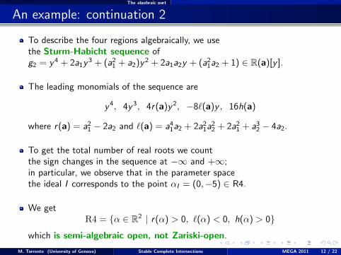
To get the total number of real roots we countthe sign changes in the sequence at −∞ and +∞;in particular, we observe that in the parameter spacethe ideal I corresponds to the point αI = (0,−5) ∈ R4.
We getR4 = {α ∈ R2 | r(α) > 0, `(α) < 0, h(α) > 0}
which is semi-algebraic open, not Zariski-open.
M. Torrente (University of Genova) Stable Complete Intersections MEGA 2011 12 / 22
The algebraic part
An example: continuation 2
To describe the four regions algebraically, we usethe Sturm-Habicht sequence ofg2 = y4 + 2a1y
3 + (a21 + a2)y2 + 2a1a2y + (a21a2 + 1) ∈ R(a)[y ].
The leading monomials of the sequence are
y4, 4y3, 4r(a)y2, −8`(a)y , 16h(a)
where r(a) = a21 − 2a2 and `(a) = a41a2 + 2a21a22 + 2a21 + a32 − 4a2.
To get the total number of real roots we countthe sign changes in the sequence at −∞ and +∞;in particular, we observe that in the parameter spacethe ideal I corresponds to the point αI = (0,−5) ∈ R4.
We getR4 = {α ∈ R2 | r(α) > 0, `(α) < 0, h(α) > 0}
which is semi-algebraic open, not Zariski-open.
M. Torrente (University of Genova) Stable Complete Intersections MEGA 2011 12 / 22
The numerical part
Admissible Perturbations
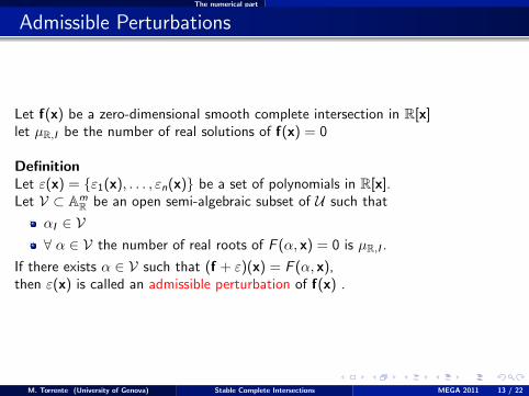
Let f(x) be a zero-dimensional smooth complete intersection in R[x]let µR,I be the number of real solutions of f(x) = 0
DefinitionLet ε(x) = {ε1(x), . . . , εn(x)} be a set of polynomials in R[x].Let V ⊂ Am
R be an open semi-algebraic subset of U such that
αI ∈ V∀ α ∈ V the number of real roots of F (α, x) = 0 is µR,I .
If there exists α ∈ V such that (f + ε)(x) = F (α, x),then ε(x) is called an admissible perturbation of f(x) .
M. Torrente (University of Genova) Stable Complete Intersections MEGA 2011 13 / 22
The numerical part
Admissible Perturbations
Let f(x) be a zero-dimensional smooth complete intersection in R[x]let µR,I be the number of real solutions of f(x) = 0
DefinitionLet ε(x) = {ε1(x), . . . , εn(x)} be a set of polynomials in R[x].Let V ⊂ Am
R be an open semi-algebraic subset of U such that
αI ∈ V∀ α ∈ V the number of real roots of F (α, x) = 0 is µR,I .
If there exists α ∈ V such that (f + ε)(x) = F (α, x),then ε(x) is called an admissible perturbation of f(x) .
M. Torrente (University of Genova) Stable Complete Intersections MEGA 2011 13 / 22
The numerical part
Example of admissible perturbation
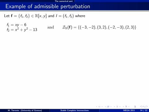
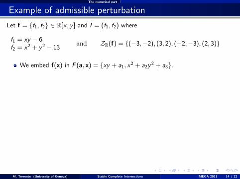
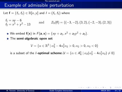
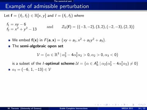
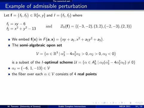
Let f = {f1, f2} ∈ R[x , y ] and I = (f1, f2) where
f1 = xy − 6f2 = x2 + y2 − 13
and ZR(f) = {(−3,−2), (3, 2), (−2,−3), (2, 3)}
We embed f(x) in F (a, x) = {xy + a1, x2 + a2y
2 + a3}.The semi-algebraic open set
V = {α ∈ R3 | α23 − 4α2
1α2 > 0, α2 > 0, α3 < 0}
is a subset of the I -optimal scheme U = {α ∈ A3R | α2(α2
3 − 4α21α2) 6= 0}
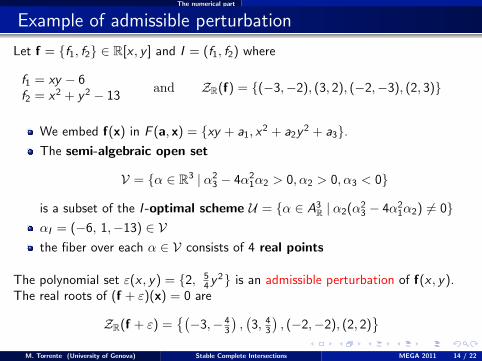
αI = (−6, 1,−13) ∈ Vthe fiber over each α ∈ V consists of 4 real points
The polynomial set ε(x , y) = {2, 54y
2} is an admissible perturbation of f(x , y).The real roots of (f + ε)(x) = 0 are
ZR(f + ε) ={(−3,− 4
3
),(3, 43
), (−2,−2), (2, 2)
}
M. Torrente (University of Genova) Stable Complete Intersections MEGA 2011 14 / 22
The numerical part
Example of admissible perturbation
Let f = {f1, f2} ∈ R[x , y ] and I = (f1, f2) where
f1 = xy − 6f2 = x2 + y2 − 13
and ZR(f) = {(−3,−2), (3, 2), (−2,−3), (2, 3)}
We embed f(x) in F (a, x) = {xy + a1, x2 + a2y
2 + a3}.
The semi-algebraic open set
V = {α ∈ R3 | α23 − 4α2
1α2 > 0, α2 > 0, α3 < 0}
is a subset of the I -optimal scheme U = {α ∈ A3R | α2(α2
3 − 4α21α2) 6= 0}
αI = (−6, 1,−13) ∈ Vthe fiber over each α ∈ V consists of 4 real points
The polynomial set ε(x , y) = {2, 54y
2} is an admissible perturbation of f(x , y).The real roots of (f + ε)(x) = 0 are
ZR(f + ε) ={(−3,− 4
3
),(3, 43
), (−2,−2), (2, 2)
}
M. Torrente (University of Genova) Stable Complete Intersections MEGA 2011 14 / 22
The numerical part
Example of admissible perturbation
Let f = {f1, f2} ∈ R[x , y ] and I = (f1, f2) where
f1 = xy − 6f2 = x2 + y2 − 13
and ZR(f) = {(−3,−2), (3, 2), (−2,−3), (2, 3)}
We embed f(x) in F (a, x) = {xy + a1, x2 + a2y
2 + a3}.The semi-algebraic open set
V = {α ∈ R3 | α23 − 4α2
1α2 > 0, α2 > 0, α3 < 0}
is a subset of the I -optimal scheme U = {α ∈ A3R | α2(α2
3 − 4α21α2) 6= 0}
αI = (−6, 1,−13) ∈ V
the fiber over each α ∈ V consists of 4 real points
The polynomial set ε(x , y) = {2, 54y
2} is an admissible perturbation of f(x , y).The real roots of (f + ε)(x) = 0 are
ZR(f + ε) ={(−3,− 4
3
),(3, 43
), (−2,−2), (2, 2)
}
M. Torrente (University of Genova) Stable Complete Intersections MEGA 2011 14 / 22
The numerical part
Example of admissible perturbation
Let f = {f1, f2} ∈ R[x , y ] and I = (f1, f2) where
f1 = xy − 6f2 = x2 + y2 − 13
and ZR(f) = {(−3,−2), (3, 2), (−2,−3), (2, 3)}
We embed f(x) in F (a, x) = {xy + a1, x2 + a2y
2 + a3}.The semi-algebraic open set
V = {α ∈ R3 | α23 − 4α2
1α2 > 0, α2 > 0, α3 < 0}
is a subset of the I -optimal scheme U = {α ∈ A3R | α2(α2
3 − 4α21α2) 6= 0}
αI = (−6, 1,−13) ∈ Vthe fiber over each α ∈ V consists of 4 real points
The polynomial set ε(x , y) = {2, 54y
2} is an admissible perturbation of f(x , y).The real roots of (f + ε)(x) = 0 are
ZR(f + ε) ={(−3,− 4
3
),(3, 43
), (−2,−2), (2, 2)
}
M. Torrente (University of Genova) Stable Complete Intersections MEGA 2011 14 / 22
The numerical part
Example of admissible perturbation
Let f = {f1, f2} ∈ R[x , y ] and I = (f1, f2) where
f1 = xy − 6f2 = x2 + y2 − 13
and ZR(f) = {(−3,−2), (3, 2), (−2,−3), (2, 3)}
We embed f(x) in F (a, x) = {xy + a1, x2 + a2y
2 + a3}.The semi-algebraic open set
V = {α ∈ R3 | α23 − 4α2
1α2 > 0, α2 > 0, α3 < 0}
is a subset of the I -optimal scheme U = {α ∈ A3R | α2(α2
3 − 4α21α2) 6= 0}
αI = (−6, 1,−13) ∈ Vthe fiber over each α ∈ V consists of 4 real points
The polynomial set ε(x , y) = {2, 54y
2} is an admissible perturbation of f(x , y).The real roots of (f + ε)(x) = 0 are
ZR(f + ε) ={(−3,− 4
3
),(3, 43
), (−2,−2), (2, 2)
}M. Torrente (University of Genova) Stable Complete Intersections MEGA 2011 14 / 22
The numerical part
Local Condition Number
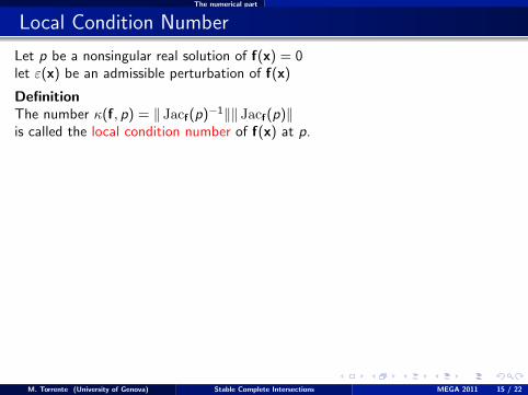
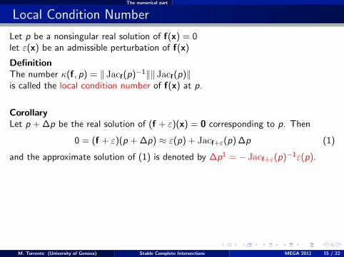
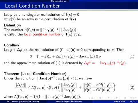
Let p be a nonsingular real solution of f(x) = 0let ε(x) be an admissible perturbation of f(x)
DefinitionThe number κ(f, p) = ‖ Jacf(p)−1‖‖ Jacf(p)‖is called the local condition number of f(x) at p.
CorollaryLet p + ∆p be the real solution of (f + ε)(x) = 0 corresponding to p. Then
0 = (f + ε)(p + ∆p) ≈ ε(p) + Jacf+ε(p) ∆p (1)
and the approximate solution of (1) is denoted by ∆p1 = − Jacf+ε(p)−1ε(p).
Theorem (Local Condition Number)Under the condition ‖ Jacf(p)−1 Jacε(p)‖ < 1, we have
‖∆p1‖‖p‖
≤ Λ(f, ε, p) κ(f, p)
(‖ Jacε(p)‖‖ Jacf(p)‖
+‖ε(0)− ε≥2(0, p)‖‖f(0)− f≥2(0, p)‖
)(2)
where Λ(f, ε, p) = 1/(1− ‖ Jacf(p)−1 Jacε(p)‖).
M. Torrente (University of Genova) Stable Complete Intersections MEGA 2011 15 / 22
The numerical part
Local Condition Number
Let p be a nonsingular real solution of f(x) = 0let ε(x) be an admissible perturbation of f(x)
DefinitionThe number κ(f, p) = ‖ Jacf(p)−1‖‖ Jacf(p)‖is called the local condition number of f(x) at p.
CorollaryLet p + ∆p be the real solution of (f + ε)(x) = 0 corresponding to p. Then
0 = (f + ε)(p + ∆p) ≈ ε(p) + Jacf+ε(p) ∆p (1)
and the approximate solution of (1) is denoted by ∆p1 = − Jacf+ε(p)−1ε(p).
Theorem (Local Condition Number)Under the condition ‖ Jacf(p)−1 Jacε(p)‖ < 1, we have
‖∆p1‖‖p‖
≤ Λ(f, ε, p) κ(f, p)
(‖ Jacε(p)‖‖ Jacf(p)‖
+‖ε(0)− ε≥2(0, p)‖‖f(0)− f≥2(0, p)‖
)(2)
where Λ(f, ε, p) = 1/(1− ‖ Jacf(p)−1 Jacε(p)‖).M. Torrente (University of Genova) Stable Complete Intersections MEGA 2011 15 / 22
The numerical part
Generalization of the Linear Case
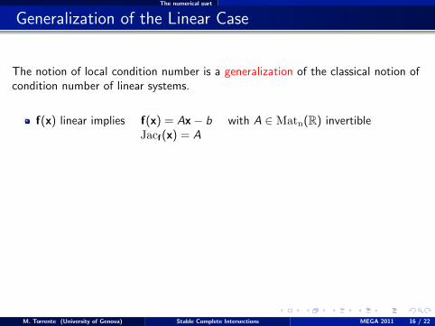
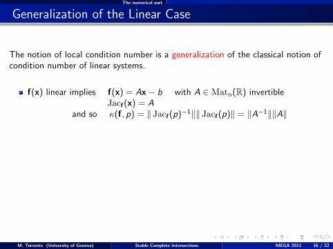
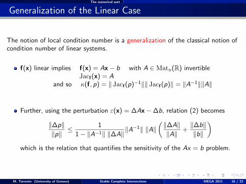
The notion of local condition number is a generalization of the classical notion ofcondition number of linear systems.
f(x) linear implies f(x) = Ax− b with A ∈ Matn(R) invertibleJacf(x) = A
and so κ(f, p) = ‖ Jacf(p)−1‖‖ Jacf(p)‖ = ‖A−1‖‖A‖
Further, using the perturbation ε(x) = ∆Ax−∆b, relation (2) becomes
‖∆p‖‖p‖
≤ 1
1− ‖A−1‖ ‖∆A‖‖A−1‖ ‖A‖
(‖∆A‖‖A‖
+‖∆b‖‖b‖
)which is the relation that quantifies the sensitivity of the Ax = b problem.
M. Torrente (University of Genova) Stable Complete Intersections MEGA 2011 16 / 22
The numerical part
Generalization of the Linear Case
The notion of local condition number is a generalization of the classical notion ofcondition number of linear systems.
f(x) linear implies f(x) = Ax− b with A ∈ Matn(R) invertibleJacf(x) = A
and so κ(f, p) = ‖ Jacf(p)−1‖‖ Jacf(p)‖ = ‖A−1‖‖A‖
Further, using the perturbation ε(x) = ∆Ax−∆b, relation (2) becomes
‖∆p‖‖p‖
≤ 1
1− ‖A−1‖ ‖∆A‖‖A−1‖ ‖A‖
(‖∆A‖‖A‖
+‖∆b‖‖b‖
)which is the relation that quantifies the sensitivity of the Ax = b problem.
M. Torrente (University of Genova) Stable Complete Intersections MEGA 2011 16 / 22
The numerical part
Further properties and Optimization
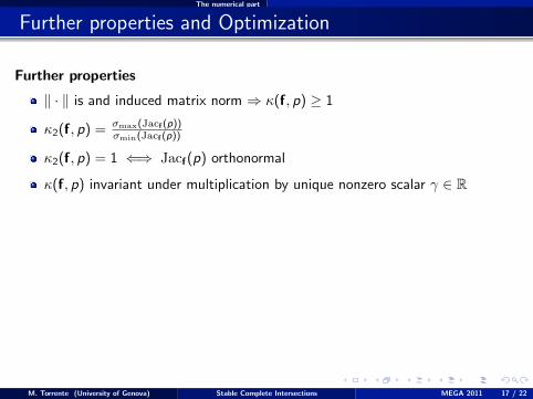
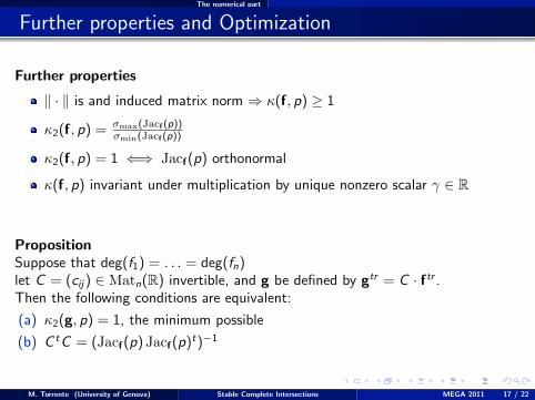
Further properties
‖ · ‖ is and induced matrix norm ⇒ κ(f, p) ≥ 1
κ2(f, p) = σmax(Jacf (p))σmin(Jacf (p))
κ2(f, p) = 1 ⇐⇒ Jacf(p) orthonormal
κ(f, p) invariant under multiplication by unique nonzero scalar γ ∈ R
PropositionSuppose that deg(f1) = . . . = deg(fn)let C = (cij) ∈ Matn(R) invertible, and g be defined by gtr = C · ftr .Then the following conditions are equivalent:
(a) κ2(g, p) = 1, the minimum possible
(b) C tC = (Jacf(p) Jacf(p)t)−1
M. Torrente (University of Genova) Stable Complete Intersections MEGA 2011 17 / 22
The numerical part
Further properties and Optimization
Further properties
‖ · ‖ is and induced matrix norm ⇒ κ(f, p) ≥ 1
κ2(f, p) = σmax(Jacf (p))σmin(Jacf (p))
κ2(f, p) = 1 ⇐⇒ Jacf(p) orthonormal
κ(f, p) invariant under multiplication by unique nonzero scalar γ ∈ R
PropositionSuppose that deg(f1) = . . . = deg(fn)let C = (cij) ∈ Matn(R) invertible, and g be defined by gtr = C · ftr .Then the following conditions are equivalent:
(a) κ2(g, p) = 1, the minimum possible
(b) C tC = (Jacf(p) Jacf(p)t)−1
M. Torrente (University of Genova) Stable Complete Intersections MEGA 2011 17 / 22
Experiments
Experiments I
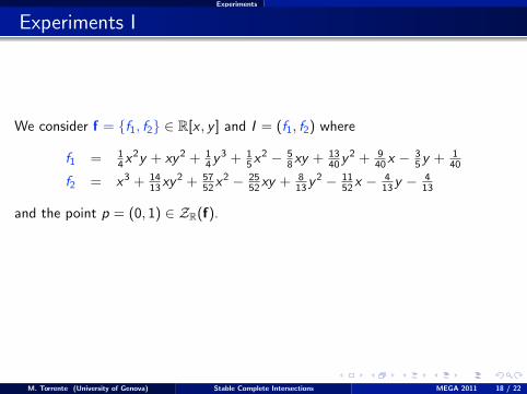
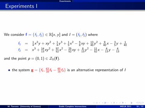
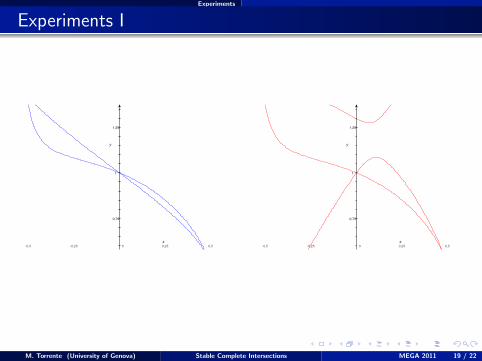
We consider f = {f1, f2} ∈ R[x , y ] and I = (f1, f2) where
f1 = 14x
2y + xy2 + 14y
3 + 15x
2 − 58xy + 13
40y2 + 9
40x −35y + 1
40
f2 = x3 + 1413xy
2 + 5752x
2 − 2552xy + 8
13y2 − 11
52x −413y −
413
and the point p = (0, 1) ∈ ZR(f).
the system g = {f1, 6316 f1 −6516 f2} is an alternative representation of I
M. Torrente (University of Genova) Stable Complete Intersections MEGA 2011 18 / 22
Experiments
Experiments I
-0,5 -0,25 0 0,25 0,5
0,75
1
1,25
-0,5 -0,25 0 0,25 0,5
0,75
1
1,25
M. Torrente (University of Genova) Stable Complete Intersections MEGA 2011 19 / 22
Experiments
Experiments I
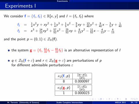
We consider f = {f1, f2} ∈ R[x , y ] and I = (f1, f2) where
f1 = 14x
2y + xy2 + 14y
3 + 15x
2 − 58xy + 13
40y2 + 9
40x −35y + 1
40
f2 = x3 + 1413xy
2 + 5752x
2 − 2552xy + 8
13y2 − 11
52x −413y −
413
and the point p = (0, 1) ∈ ZR(f).
the system g = {f1, 6316 f1 −6516 f2} is an alternative representation of I
q ∈ ZR(f + ε) and r ∈ ZR(g + ε) are perturbations of pfor different admissible perturbations ε
κ2(f, p) ‖q−p‖2‖p‖2
8 0.000097
κ2(g, p) ‖r−p‖2‖p‖2
1 0.000023
M. Torrente (University of Genova) Stable Complete Intersections MEGA 2011 20 / 22
Experiments
Experiments II
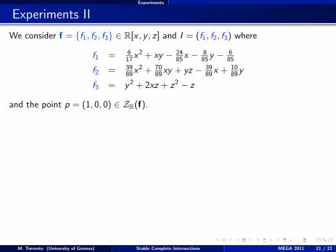
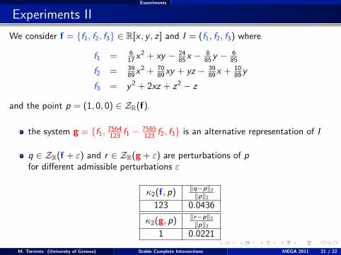
We consider f = {f1, f2, f3} ∈ R[x , y , z ] and I = (f1, f2, f3) where
f1 = 617x
2 + xy − 2485x −
885y −
685
f2 = 3989x
2 + 7089xy + yz − 39
89x + 1089y
f3 = y2 + 2xz + z2 − z
and the point p = (1, 0, 0) ∈ ZR(f).
the system g = {f1, 7564123 f1 −7565123 f2, f3} is an alternative representation of I
q ∈ ZR(f + ε) and r ∈ ZR(g + ε) are perturbations of pfor different admissible perturbations ε
κ2(f, p) ‖q−p‖2‖p‖2
123 0.0436
κ2(g, p) ‖r−p‖2‖p‖2
1 0.0221
M. Torrente (University of Genova) Stable Complete Intersections MEGA 2011 21 / 22
Experiments
Experiments II
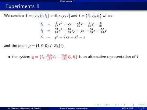
We consider f = {f1, f2, f3} ∈ R[x , y , z ] and I = (f1, f2, f3) where
f1 = 617x
2 + xy − 2485x −
885y −
685
f2 = 3989x
2 + 7089xy + yz − 39
89x + 1089y
f3 = y2 + 2xz + z2 − z
and the point p = (1, 0, 0) ∈ ZR(f).
the system g = {f1, 7564123 f1 −7565123 f2, f3} is an alternative representation of I
q ∈ ZR(f + ε) and r ∈ ZR(g + ε) are perturbations of pfor different admissible perturbations ε
κ2(f, p) ‖q−p‖2‖p‖2
123 0.0436
κ2(g, p) ‖r−p‖2‖p‖2
1 0.0221
M. Torrente (University of Genova) Stable Complete Intersections MEGA 2011 21 / 22
Future work
Future work
Optimization in the case of arbitrary degrees
Definition of global condition number
. . .
Thank you!
M. Torrente (University of Genova) Stable Complete Intersections MEGA 2011 22 / 22

Future work
Future work
Optimization in the case of arbitrary degrees
Definition of global condition number
. . .
Thank you!
M. Torrente (University of Genova) Stable Complete Intersections MEGA 2011 22 / 22