Stability Criteria for theContextual Emergence of Macrostates

in Neural Networks

Peter beim Graben∗

School of Psychology and Clinical Language Sciences,University of Reading, UK

Adam BarrettDepartment of Informatics,University of Sussex, UK

Harald AtmanspacherInstitute for Frontier Areas of Psychology and Mental Health,

Freiburg, Germany

July 2, 2009

Accepted Manuscript to appear in Network: Computation in Neural Sys-tems.

Abstract

More than thirty years ago, Amari and colleagues proposed a sta-tistical framework for identifying structurally stable macrostates ofneural networks from observations of their microstates. We comparetheir stochastic stability criterion with a deterministic stability crite-rion based on the ergodic theory of dynamical systems, recently pro-posed for the scheme of contextual emergence and applied to particu-lar inter-level relations in neuroscience. Stochastic and deterministic

∗Email: p.r.beimgraben@reading.ac.uk

1

stability criteria for macrostates rely on macro-level contexts, whichmake them sensitive to differences between different macro-levels.

1 Introduction

One of the most important issues in neuroscience are relations between differ-ent levels of description. In cognitive neuroscience, this refers to the relation-ship between the brain states and their dynamics and mental states relevantfor phenomena such as cognition and even consciousness at a higher level.Corresponding ideas have been put forward, e.g., by Smolensky (1988, 2006),beim Graben (2004) and Atmanspacher and beim Graben (2007) for the rela-tionship between neurodynamics on the one hand and cognitive computationor mental states in general on the other.

In computational neuroscience, relations between microscopic states (ofion channels, individual neurons, synapses), mesoscopic states (of neural as-semblies, cortical columns) and macroscopic states (of functional networks asobservable by techniques such as EEG or fMRI) and their associated levelsof description are concerned. A recent review by Atmanspacher and Rotter(2008) outlines numerous examples, achievements and problems for specificinter-level relations between descriptions of the brain and its components.

Inter-level relations in general have been a topic of discussion for decades,and key questions have not been ultimately resolved even today. Are higher-level descriptions strongly reducible to lower-level descriptions? Do higher-level descriptions supervene upon lower-level descriptions? Or do higher-leveldescriptions emerge from lower-level descriptions?

Recently, Bishop and Atmanspacher (2006) suggested a classification ofinter-level relations in terms of necessary and sufficient conditions. If a lower-level description bears both necessary and sufficient conditions for a higher-level description, the higher level can be strongly reduced to the lower level.If a lower-level description possesses sufficient but not necessary conditionsfor a higher-level description, the latter supervenes upon the former. Forsituations in which a lower-level description is necessary but not sufficientfor a higher-level description, Bishop and Atmanspacher (2006) propose theterm contextual emergence. The remaining, rather unattractive, case in whichthe lower-level description provides neither necessary nor sufficient conditionsfor the higher level description has been called radical emergence, resembling

2

a patchwork scenario with basically unrelated domains.

The idea of contextual emergence has been successfully used to clarifyinter-level relations between statistical mechanics and thermodynamics andbetween quantum mechanics and physical chemistry (Primas 1998, Bishopand Atmanspacher 2006). It has also been shown to be a viable tool toformally address neural correlates of consciousness (Chalmers 2000) in termsof partitioned neural state spaces (Atmanspacher and beim Graben 2007).This methodology, which is based on the ergodic theory of deterministicdynamical systems, can also be applied to study relations between the (lower-level) dynamics of neural networks and the (higher-level) behavior of localfield potentials or the EEG (Allefeld et al. 2009).

It is the aim of this paper to demonstrate that elements of the same kindof contextual emergence are applicable, and in fact have been applied earlier,to inter-level relations between statistical descriptions of neural systems. Re-markably, the basic ingredients for such an investigation have been workedout more than thirty years ago by Amari (1974) and Amari et al. (1977) intwo influential papers on macrostates in random neural networks.

Referring to higher-level states as macrostates and lower-level states asmicrostates, Amari (1974, p. 203) introduced a theory of statistical neurody-namics in the following way:

“Statistical neurodynamics investigates such properties of ran-dom nets that are possessed in common by almost all randomnets in an ensemble rather than those that are possessed on theaverage. When random nets are composed of a sufficiently largenumber of neurons, it is anticipated from the law of large num-bers that such properties surely exist. These properties, if theyexist, do not depend on the precise values of net parameters butonly on their statistics. They are structurally stable in the sensethat a minor change of parameters do not destroy the properties.These properties are analyzed in the following by introducing theconcept of macrostates.”

The paper is structured as follows: In Sect. 2 we review the contextualemergence of (higher-level) macrostates and their associated properties from(lower-level) microstates and their associated properties. Particular empha-sis is placed on the issue of structural stability, referred to in the quotation

3

above. In Sect. 3 we demonstrate contextual emergence in neural networksin three steps. In a first step (Sect. 3.1) we recapitulate Amari’s approach bytranslating his original formalism in the light of algebraic statistical mechan-ics (Sewell 2002) and dynamical system theory (Guckenheimer and Holmes1983). In a second step (Sect. 3.2) we introduce the notion of contextual-ity by epistemic observables in the sense of beim Graben and Atmanspacher(2006). In a third step (Sect. 3.3) we show how Amari’s macrostate criteriaimplement appropriate stability conditions for the contextual emergence ofmacroscopic descriptions for a random neural network.

The paper concludes with a discussion of similarities and differences ofthe approaches. In addition, a particular example is addressed, contextualemergence of macrostates in liquid state machines (Maass et al. 2002) thatmight be relevant for the discussion of neural correlates of consciousness(Chalmers 2000, Atmanspacher and beim Graben 2007).

2 Contextual Emergence: The Basic Idea

For the idea of contextual emergence it is assumed that the description offeatures of a system at a particular level offers necessary but not sufficientconditions to derive features at a higher level of description. In logical terms,the necessity of conditions at the lower level of description means that higher-level features imply those of the lower level of description. The converse —that lower-level features also imply the features at the higher level of descrip-tion — does not hold in contextual emergence. This is the meaning of theabsence of sufficient conditions at the lower level of description. Additional,contingent contexts for the transition from the lower to the higher level ofdescription are required in order to provide such sufficient conditions.

For the contextual emergence of temperature, the notion of thermal equi-librium represents such a context. Thermal equilibrium is not available atthe lower-level description of Newtonian or statistical mechanics. Imple-menting thermal equilibrium in terms of a particular stability condition (theKubo-Martin-Schwinger (KMS) condition) and considering the thermody-namic limit of infinitely many particles (N → ∞) at the level of statisticalmechanics, temperature can be obtained as an emergent property at a higher-level thermodynamical description.1 It is of paramount importance for this

1A non-technical presentation of the detailed argumentation can be found in At-

4

procedure that KMS states satisfy a stability condition that derives froma context at the level of thermodynamics and implemented at the level ofstatistical mechanics.

In addition to the contextual emergence of temperature as a new observ-able that is not contained in the algebra of observables of statistical mechan-ics, the concept of a thermal state differs substantially from the concept of astatistical state. The introduction of KMS states in the phase space of statis-tical mechanics entails a coarse graining (a change of topology) that leads toequivalence classes of microstates with properties implying the same temper-ature. These equivalent microstates are multiple realizations of one and thesame thermal state. In this sense, thermal states supervene on microstates,although thermal properties emerge from properties of microstates.

The significance of contextual emergence in combination with superve-nience as opposed to strict reduction in this example is clear. Of course,it would be interesting to extend the general construction scheme outlinedabove to other cases. More physical examples are indicated and discussed,for example, in Primas (1998) and Batterman (2002). However, the conceptof stability, in the sense of stability against perturbations or fluctuations,should serve as a key principle for the construction of a contextual topologyand an associated algebra of contextual observables in examples even beyondphysics.

As mentioned in the introduction, possible, and ambitious, cases referto emergent features in the framework of cognitive science and neuroscience(Atmanspacher 2007). As the brain definitely operates far from equilibrium,the general approach must be able to incorporate a non-equilibrium stabil-ity criterion. Based on empirical material that suggests to consider neuro-dynamics in terms of deterministic nonlinear dynamics, Atmanspacher andbeim Graben (2007) suggested a suitable implementation, based on ergodictheory, of appropriate higher-level contexts as lower-level stability conditions.

Depending on the precise nature of the dynamics, basins of attraction(e.g., for fixed points) or invariant hyperbolic sets (e.g., for chaotic attractors)provide partitions of the phase space. These coarse-grainings are directlyprescribed by the deterministic dynamics of the system considered and canbe investigated in terms of ergodic Markov chains (see appendix). At the

manspacher (2007). The KMS condition induces a partition into equivalence classes ofmechanical states defining statistical states whose mean energy can be assigned a partic-ular temperature.

5

higher level of description, the coarse grains or partition cells represent new(macro-) states with new associated observables, respectively.

3 Emergence of Macrostates

in Neural Networks

In this section we demonstrate how Amari’s macrostate criteria for statisticalneurodynamics (Amari 1974, Amari et al. 1977) compares to macrostatecriteria for the contextual emergence of macroscopic descriptions for neuralnetworks.

3.1 Amari’s Macrostate Conditions

Amari (1974) and Amari et al. (1977) discussed ensembles of random (orstochastic) networks of McCulloch-Pitts units.2 This can be formalized bya phase space Xn ⊂ Rn of n randomly connected model neurons, obeying anonlinear difference equation:

x(t+ 1) = Φω(x(t)) . (1)

Here x(t) ∈ Xn is the activation vector (the microstate) of the network attime t and Φω is a nonlinear map, parameterized by ω. The network as adynamical system is then given by (Xn,Φω).

The map Φω is often assumed to be of the form

Φω(x) = f(W · x− θ) , (2)

with synaptic weight matrix W ∈ Rn2, activation threshold vector θ ∈ Rn,

and a nonlinear squashing function f = (fi)1≤i≤n : Xn → Xn, the activationfunction of the network. For fi = Θ (where Θ denotes the Heaviside jumpfunction), equations (1, 2) describe a network of McCulloch-Pitts neurons(McCulloch and Pitts 1943).

Another popular choice for the activation function is the logistic function

fi(x) =1

1 + e−x,

2Another important example are Hebbian auto-associator networks (Hopfield 1982)trained with random patterns that have been investigated by Amari and Maginu (1988).

6

describing firing rate models (cf., e.g., beim Graben (2008)). Replacing Eq.(2) by the map

Φω(x) = (1−∆t)x+ ∆tf(W · x− θ) (3)

yields a time-discrete leaky integrator network (Wilson and Cowan 1972,beim Graben and Kurths 2008). For numerical simulations, ∆t < 1 will bethe choice for the time step of the Euler method.

According to (2) and (3), the network parameters are given as

ω = (W ,θ) ∈ Rn2 × Rn . (4)

In a random neural network, the parameters ω are regarded as stochasticvariables drawn from a probability space Ωn = Rn2 × Rn with measure

µn : B(Ωn)→ [0, 1] (5)

for measurable sets from B(Ωn). We refer to a particular network realizationfrom this probability space as N(ω).

In order to obtain limit theorems for random neural networks, one has toassure that network realizations of different size n behave similarly. Thus, werestrict ourselves to particular network topologies, such as directed Erdos-Renyi graphs with fixed connectivity p (Bollobas 2001, beim Graben andKurths 2008, Maass et al. 2002) or networks with Gaussian synaptic weightsW ∼ N (m, nσ2). For an Erdos-Renyi network of size n the expected numberof connections is then np.

Amari (1974) and Amari et al. (1977) treat the network parameters ωas strictly stochastic variables, such that the evolution equations (2) and(3) describe stochastic processes where ω assumes another value after eachtemporal iteration. Amari (1974, p. 203) concedes that such an “ensemble ofrandom nets is quite different to the Gibbs ensemble in statistical mechanicsin this respect, because the latter consists of dynamical systems of the samestructure but only in different states”.

Simplifying Amari’s treatment of networks, we follow Amari and Maginu(1988) and Touboul et al. (2008) who describe a random neural network asone particular realization of the stochastic variable ω that is considered frozenduring the temporal evolution of the network states. This assumption doesnot only facilitate the theory, it is also more plausible for certain scenarios.The changes of network parameters during development usually take place

7

at a larger time scale than the intrinsic network dynamics. Note, however,that time scales related to synaptic plasticity cannot always be separated soeasily.

Touboul et al. (2008) also consider noise-driven networks, which wouldagain require a fully stochastic treatment. We will refrain from this com-plication as well and study random neural networks in the original sense ofGibbs ensembles, namely as ensembles of identical systems (characterizedby the same realization of the stochastic parameter ω for a given networksize n). Such systems differ only in their initial conditions. This approachis consistent with the treatment of deterministic dynamical systems whereinitial conditions can be drawn according to probability distributions overphase space. Particular distributions, so-called Sinai-Ruelle-Bowen (SRB)measures (Guckenheimer and Holmes 1983), obey stability conditions thatare crucial for the contextual emergence of macrostates in dynamical systems.

A macro-observable of a neural network (Xn,Φω) is a real-valued functions : Xn → R that is measurable by suitable techniques. Such observables are,e.g., local field potentials or the EEG (Freeman 2007). Let si;n : Xn → R bea family of m observables (for 1 ≤ i ≤ m) for a network of size n, such thaty = sn(x) = (si;n(x))1≤i≤m is a vector in m-dimensional space Y ⊂ Rm. Wecall Y = sn(Xn) the macrostate space generated by the family (si;n)1≤i≤m.Note that we are interested in a macrostate space Y that is the same for asequence of network realizations (Xn,Φω)n∈N.

Amari (1974) and Amari et al. (1977) asked for conditions under whichthe images y = sn(x) of a microstate x under the observables sn can be re-garded as macrostates obeying a macroscopic evolution law. In order to for-mulate appropriate constraints, Amari (1974, p. 203) discussed two possibleconditions which should be fulfilled if the number n of network componentsis sufficiently large:3

1. In order for sn(x) to represent a macrostate whose state-transitionlaw is identical for almost all nets, it is required that the values ofy(1) = sn(Φω(x(0))) are identical for almost all nets in the ensemble,even though the values of Φω(x(0)) differ for different N(ω)’s.

2. The value of the macrostate y(1) = sn(Φω(x(0))) is required to dependon x(0) not directly but only through the value of the initial macrostatey(0) = sn(x(0)).

3We present Amari’s proposal in our own notation here and in the following.

8

Amari (1974, pp. 203f) proposed that these verbal criteria give rise to thefollowing formal macrostate condition (see also Amari et al. (1977, p. 98)):The images y = sn(x) of microstates x under the sequence of observablessn is called a macrostate if it fulfils, for every x ∈ Xn, the following criteria:

1. There exists a function ϕ : Y → Y for which

limn→∞

Eµn(sn(Φω(x))) = ϕ(sn(x)) . (6)

2. And, furthermore

limn→∞

Vµn(||sn(Φω(x))||) = 0 . (7)

Here, Eµn and Vµn denote, respectively, the ensemble mean and ensem-ble variance (i.e., the expectation and variance of stochastic variables withrespect to the probability measure µn), and the Euclidian norm

||y||2 =m∑i=1

y2i .

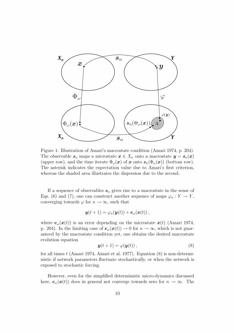
The macrostate condition formulated by Eqs. (6,7) can be graphicallydepicted as a diagram that is asymptotically (n → ∞) commutative (Fig.1). Note that a similar quasi-commutativity has been observed by Gaveauand Schulman (2005) for the coarse-graining of Markov chains.

9

Xn

Xn

Y

Y

Figure 1: Illustration of Amari’s macrostate condition (Amari 1974, p. 204).The observable sn maps a microstate x ∈ Xn onto a macrostate y = sn(x)(upper row), and the time iterate Φω(x) of x onto sn(Φω(x)) (bottom row).The asterisk indicates the expectation value due to Amari’s first criterion,whereas the shaded area illustrates the dispersion due to the second.

If a sequence of observables sn gives rise to a macrostate in the sense ofEqs. (6) and (7), one can construct another sequence of maps ϕn : Y → Y ,converging towards ϕ for n→∞, such that

y(t+ 1) = ϕn(y(t)) + eω(x(t)) ,

where eω(x(t)) is an error depending on the microstate x(t) (Amari 1974,p. 204). In the limiting case of eω(x(t))→ 0 for n→∞, which is not guar-anteed by the macrostate condition yet, one obtains the desired macrostateevolution equation

y(t+ 1) = ϕ(y(t)) , (8)

for all times t (Amari 1974, Amari et al. 1977). Equation (8) is non-determi-nistic if network parameters fluctuate stochastically, or when the network isexposed to stochastic forcing.

However, even for the simplified deterministic micro-dynamics discussedhere, eω(x(t)) does in general not converge towards zero for n → ∞. The

10

reason are temporal correlations in x(t). An illustrative example is a Hop-field network trained on random patterns, discussed by Amari and Maginu(1988). This makes Amari’s macrostate criteria (6) and (7) necessary butnot sufficient conditions for the macrostate dynamics (8). As a sufficientcondition Amari (1974, p. 204) postulates

limn→∞

Prob

supt||sn(Φt

ω(x(0)))− ϕt(x(0))|| > ε

= 0 (9)

for arbitrary ε > 0.

Since Eq. (9) refers to the images of microstates in macrostate space un-der the observables sn it can be regarded as a decorrelation condition. Amari(1974) compares Eq. (9) with Boltzmann’s Stoßzahlansatz in statistical me-chanics. Amari et al. (1977) proved Eq. (9) under several assumptions aboutthe microscopic dynamics.

3.2 Contextual Observables

Any real-valued function s : Xn → R of a neural network (Xn,Φω) that canbe measured is an observable. Since observables are usually defined withrespect to a particular scientific or pragmatic context (Freeman 2007), werefer to them as contextual observables. A context provides a reference framefor the meaningful usage of observables.4

In general, the mapping sn : Xn → Y,x 7→ y obtained from a familysi;n : Xn → R of m observables (for 1 ≤ i ≤ m) is not injective, suchthat different neural microstates x,x′ ∈ Xn are mapped onto the same statey ∈ Y in macrostate space. Following beim Graben and Atmanspacher(2006), we call the states x,x′ ∈ X epistemically equivalent with respectto the observables si;n. Epistemic equivalence induces a partition of theneural phase spaces Xn into disjoint classes such that all members of oneclass are mapped onto the same point y in the macrostate space Y . CallAy = s−1

n (y) ⊂ Xn the equivalence class of all pre-images of y.

Arbitrarily defined observables are unlikely to obey stability conditionssuch as Amari’s macrostate condition. However, we can generally construct

4This situation resembles quantum mechanical complementarity where observables suchas the position and momentum of an electron refer to different, mutually excluding mea-surement contexts. For a treatment of complementary observables in classical systems seebeim Graben and Atmanspacher (2006).

11

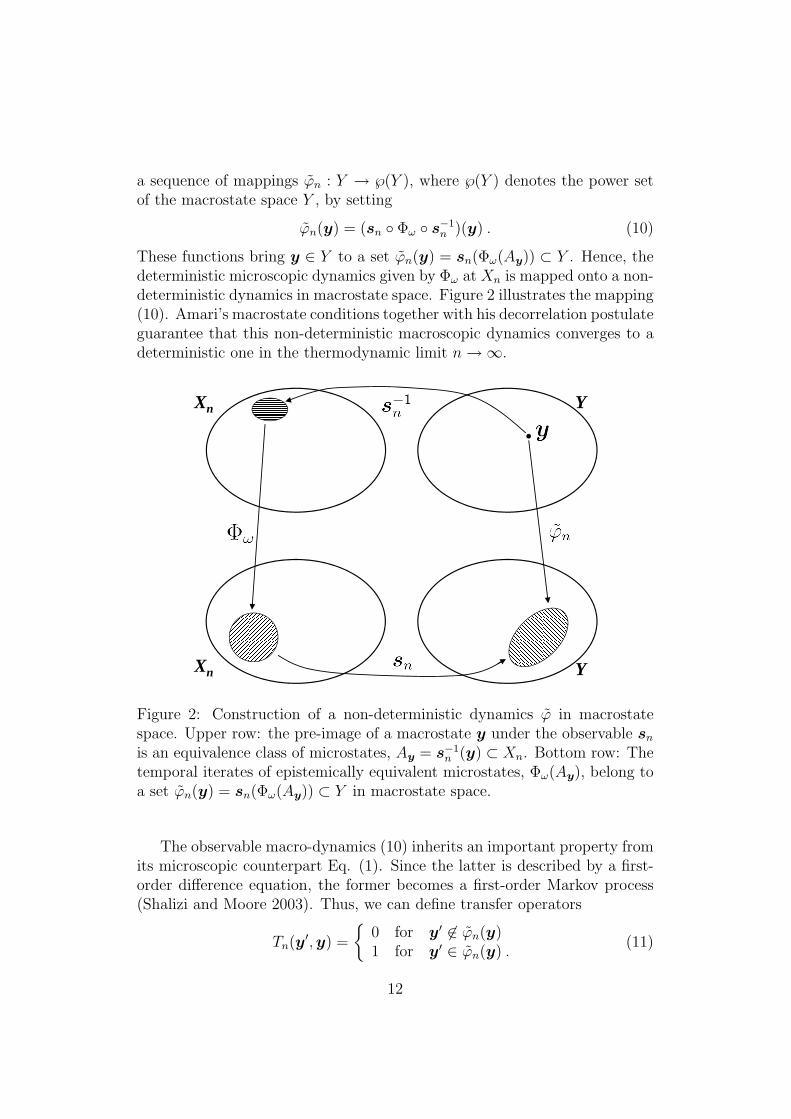
a sequence of mappings ϕn : Y → ℘(Y ), where ℘(Y ) denotes the power setof the macrostate space Y , by setting

ϕn(y) = (sn Φω s−1n )(y) . (10)

These functions bring y ∈ Y to a set ϕn(y) = sn(Φω(Ay)) ⊂ Y . Hence, thedeterministic microscopic dynamics given by Φω at Xn is mapped onto a non-deterministic dynamics in macrostate space. Figure 2 illustrates the mapping(10). Amari’s macrostate conditions together with his decorrelation postulateguarantee that this non-deterministic macroscopic dynamics converges to adeterministic one in the thermodynamic limit n→∞.

Xn

Xn

Y

Y

Figure 2: Construction of a non-deterministic dynamics ϕ in macrostatespace. Upper row: the pre-image of a macrostate y under the observable snis an equivalence class of microstates, Ay = s−1

n (y) ⊂ Xn. Bottom row: Thetemporal iterates of epistemically equivalent microstates, Φω(Ay), belong toa set ϕn(y) = sn(Φω(Ay)) ⊂ Y in macrostate space.

The observable macro-dynamics (10) inherits an important property fromits microscopic counterpart Eq. (1). Since the latter is described by a first-order difference equation, the former becomes a first-order Markov process(Shalizi and Moore 2003). Thus, we can define transfer operators

Tn(y′,y) =

0 for y′ 6∈ ϕn(y)1 for y′ ∈ ϕn(y) .

(11)

12

The transfer operators do not vanish if the state y′ ∈ Y belongs to the imageof ϕn(y), for y ∈ Y .

3.3 Structural Stability

3.3.1 Stochastic Structural Stability

In a first step, we show that Amari’s macrostate criterion entails a stochasticcondition for structural stability. To this aim, we formalize Amari’s firstverbal criterion “that the values of y(1) = sn(Φω(x(0))) are identical foralmost all nets in the ensemble, even though the values of Φω(x(0)) differ fordifferent N(ω)’s” as follows:

For all ε, δ > 0 there exists a k such that for all n > k, x ∈ Xn,

Prob||sn(Φω(x))− sn(Φω′(x))|| > ε < δ (12)

if ω and ω′ are drawn from Ωn = Rn2 × Rn using the probability measureµn. Equation (12) expresses that, for two random realizations of the mi-crostate dynamics, the macrostate dynamics will, with high probability, bevery similar if the number of neurons is large. (Note that the exact inter-pretation of (12) is slightly different from Amari’s formulation in that thevalues of y(1) = sn(Φω(x(0))) are almost identical for almost all nets in theensemble.)

Amari’s second macrostate criterion is equivalent with the probabilisticstructural stability condition (12), provided that for all ε > 0, there exists ak such that for all n > k, x ∈ Xn,

Vµn(||sn(Φω(x))||) < ε , (13)

This assertion is proved as follows: Consider a one-dimensional macrostateobeying a Gaussian distribution. (Higher-dimensional macrostates are treatedsimilarly.) Suppose S, S ′ are two one-dimensional stochastic variables, obey-ing an N (m,σ2) distribution. Then, for any ε,

Prob|S − S ′| > ε = 2

(1− F

(ε√2σ

)), (14)

13

where F is the cumulative distribution function for a N (0, 1) random vari-able. Using

zf(z)

z2 + 1< 1− F (z) <

f(z)

z, (15)

where f is the probability density function of a N (0, 1) random variable, twoinequalities follow:

Prob|S − S ′| > ε <2σ√πε

e−ε2/4σ2

, (16)

Prob|S − S ′| > ε >2σε√

π(ε2 + 2σ2)e−ε

2/4σ2

. (17)

Assume now that Amari’s macrostate criterion, as given by (13), holds.Choose any ε, δ > 0. Then, by Amari’s condition (13), and the fact thatthe RHS of (16) tends to zero as σ → 0, we can choose a k such that for anyn > k and any x ∈ Xn, stochastic structural stability (12) holds.

If, conversely, Amari’s macrostate criterion does not hold, then there is aδ > 0 such that, for any n, we can find an x ∈ Xn such that

Vµn(sn(Φω(x))) > δ . (18)

Then, since the RHS of (17) increases with σ, for any n, we can find anx ∈ Xn such that

Prob|sn(Φω(x))− sn(Φω′(x))| > ε > 2√δε√

π(ε2 + 2δ)e−ε

2/4δ . (19)

Hence, stochastic structural stability (12) fails in this case.

3.3.2 Deterministic Structural Stability

Let us now assume that the contextual observables sn partition the phasespaces Xn into a finite number ` ∈ N of epistemic equivalence classes. Then,the Markov process in macrostate space Y , described by (11), becomes afinite-state Markov chain, or, in other words, a shift of finite type (Lind andMarcus 1995). Such a non-deterministic dynamical system can be obtainedfrom a finite partition Pn = A1, . . . , A` of Xn into pairwise disjoint sub-sets Ai that cover the whole phase space Xn, by choosing the characteristicfunctions si;n = χAi

as contextual observables. Then, y = sn(x) is the `-dimensional canonical basis vector y = (0, . . . , 0, 1, 0, . . . , 0)T with 1 in theith position if x ∈ Ai.

14

Structural stability ensures that, in the limit n → ∞, there is a well-defined transfer operator (11). For shifts of finite type this is a transitionmatrix

Tik =

0 for Φω(Ak) ∩ Ai = ∅1 for Φω(Ak) ∩ Ai 6= ∅ ,

(20)

that can be regarded as an adjacency matrix of a transition graph. As in-dicated in Sect. 4, Atmanspacher and beim Graben (2007) used stabilityconditions for shifts of finite type to construct contextually emergent observ-ables from neurodynamics. If the transition matrix T = (Tik) is diagonal,there are only transitions from every state to itself, indicating fixed pointsin macrostate space. If a power T q for q ∈ N is diagonal, the correspondingMarkov chain is periodic. In both cases, the observable dynamics possessesinvariant and ergodic states that are structurally stable.

If the transition matrix T is irreducible, i.e., if a power T q > 0 for q ∈ N,the Markov chain is irreducible and aperiodic. In this case the observabledynamics possesses invariant, ergodic and mixing states (Ruelle 1968, 1989).They generalize the KMS states of algebraic statistical mechanics (Olesenand Pedersen 1978, Pinzari et al. 2000, Exel 2004) to structurally stablenon-equilibrium SRB measures in the microscopic phase spaces Xn.

Now we can identify the kind of Markov chain that is obtained for anobservable dynamics obeying both of Amari’s macrostate conditions. Sincethis condition assures the existence of the map ϕ : Y → Y , we obtain thedeterministic macrostate dynamics (8)

y(t+ 1) = ϕ(y(t))

under our simplifications and in the limit n → ∞. Thus, the pre-imageB = s−1

n (ϕ(y(t))) is again an equivalence class in phase space. This meansthat cells of the partition P = A1, . . . , A` are faithfully mapped onto cellsof the partition. The resulting shift of finite type is therefore a deterministicMarkov chain where every vertex in the transition graph is the source ofone link at most. Hence, there must be a positive integer number q makingT q diagonal. Therefore, the macroscopic dynamics is either multistable orperiodic.

We see that the restriction to deterministic microscopic dynamics yields,under Amari’s macrostate condition, a deterministic macroscopic dynamicswhich is a shift of finite type for a finite number of distinct macrostates. Asa consequence we obtain structurally stable fixed points or limit tori in themacrostate space as contextually emergent macro-features.

15

However, it is straightforward to relax Amari’s macrostate condition toMarkovian macrostate dynamics by demanding Markov partitions in the mi-croscopic neural phase spaces (Sinai 1968, Ruelle 1989), but keeping thestructural stability condition. For the simplified case of expanding maps,Markov partitions have the property that cells are mapped onto joins ofcells; i.e. cell bounderies are mapped onto cell bounderies, without necessar-ily mapping cells onto cells — which was actually the result of this sectionfor deterministic Markov chains — (for hyperbolic maps things are slightlymore involved), such that Φω(Ak) ∩ Ai 6= ∅ implies Ai ⊂ Φω(Ak). Markovpartitions entail aperiodic, irreducible Markov chains, which in turn possessinvariant, ergodic and mixing SRB measures, i.e., structurally stable chaoticattractors, in the macrostate space.

3.3.3 Macrostates in a Random Neural Network

Consider a random network of n randomly connected McCulloch-Pitts units,described by Equations (1) and (2) with Heaviside activation function,

xi(t+ 1) = Θ

(n∑j=1

wijxj(t)− hn

), (21)

where 0 < h < 1. Let the synaptic weights wij be independently identicallydistributed random normal variables with mean m and variance nσ2, that is

wij ∼ N (m,nσ2) . (22)

Following Amari (1974), we can define the activity level

r(t) =1

n

n∑i=1

xi(t) (23)

of the network that serves as a kind of “model EEG”. Given an appropriatelychosen constant r0 satisfying 0 < r0 < 1, a contextual observable may bedefined by

s(t) =

0 , r(t) ≤ r0 ,r(t)− r0

1− r0, r(t) > r0

. (24)

In order to prove that s yields a macrostate satisfying the previouslydefined stability condition (13), we first determine the probability that unit

16

xi is active at time t+ 1 as

Probxi(t+ 1) = 1 = Prob

Θ

(n∑j=1

wijxj(t)− hn

)= 1

= Prob

n∑j=1

wijxj(t)− hn > 0

= Prob

n∑j=1

wijxj(t) > hn

.

Since xj(t) ∈ 0, 1 for all times t, the weighted sum

n∑j=1

wijxj(t) =∑jk

wijk ,

when xjk(t) = 1. Now, the number of active units jk at time t is giventhrough the activity level as nr(t). Because the synaptic weights wij are nor-mally distributed according to N (m,nσ2), their sum is normally distributedaccording to N (mnr(t), n2σ2r(t)). Thus,

Probxi(t+ 1) = 1 = Prob

N (0, 1) >

h−mr(t)σ√r(t)

.

On the other hand, the activity level (23) is described by a Bernoulliprocess obeying a binomial distribution

nr(t+ 1) ∼ B(n, q(t)) ,

where B(n, q(t)) denotes the binomial distribution with n trials and proba-bility q for a positive outcome in each trial, with

q(t) = π(r(t)) = 1− F

(h−mr(t)σ√r((t)

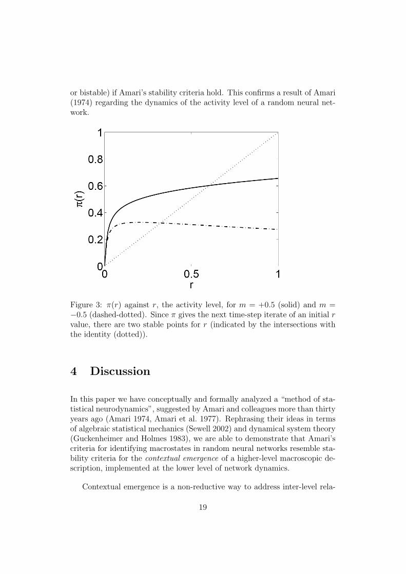
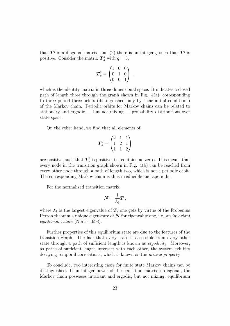
)with F being the cumulative standard normal distribution function as above.Note that π : [0, 1] → [0, 1] satisfies π(0) = 0, π(r) > 0 for r > 0, andπ′(r) → +∞ as r → 0. See Figure 3 for typical plots of π against r forpositive and negative m.

In the case m > 0, let r∗ be the larger solution of

π(r) = r ,

17

while we define for m < 0

r∗ = maxr∈[0,1]

(π(r)) .

Choose now ε > 0 and δ > 0, and let us consider the uncertainty ins(t + 1) given s(t). Suppose that s(t) = 0 initially, which is consistent withr(t) ≤ r0. Then, for n sufficiently large,

Prob s(t+ 1) > ε = Prob nr(t+ 1) > n(r0 + ε(1− r0))= Prob B(n, π(r(t))) > n(r0 + ε(1− r0))

≈ Prob

N (0, 1) >

√nr0 − π(r(t)) + ε(1− r0)√

π(r(t))[1− π(r(t))]

< δ , (25)

under the conditionr0 ≥ r∗ . (26)

Moreover, if r(t) > r0, then for n sufficiently large,

Prob |s(t+ 1)− Eµn [s(t+ 1)]| > ε < Prob |s(t+ 1)− Eµn [s(t+ 1)]| > ε(1− r0)

= 2 Prob

N (0, 1) >

√nε√

π(r(t))[1− π(r(t))]

< δ . (27)

Combining these inequalities, we deduce that there exists a k such thatfor all n > k, and all possible initial microstates x(t) ∈ Xn,

Prob |s(t+ 1)− Eµn [s(t+ 1)]| > ε < δ . (28)

This is sufficient for the observable s to yield well-defined macrostates ac-cording to Amari’s stability criteria.

For another coarse-grained contextual observable

s(x) =

0 , r(x) ≤ r0 ,1 , r(x) > r0 ,

(29)

the same argument holds for all possible initial microstates x(t) ∈ Xn.The observable s provides a Markov chain that is periodic (either mono-

18

or bistable) if Amari’s stability criteria hold. This confirms a result of Amari(1974) regarding the dynamics of the activity level of a random neural net-work.

Figure 3: π(r) against r, the activity level, for m = +0.5 (solid) and m =−0.5 (dashed-dotted). Since π gives the next time-step iterate of an initial rvalue, there are two stable points for r (indicated by the intersections withthe identity (dotted)).

4 Discussion

In this paper we have conceptually and formally analyzed a “method of sta-tistical neurodynamics”, suggested by Amari and colleagues more than thirtyyears ago (Amari 1974, Amari et al. 1977). Rephrasing their ideas in termsof algebraic statistical mechanics (Sewell 2002) and dynamical system theory(Guckenheimer and Holmes 1983), we are able to demonstrate that Amari’scriteria for identifying macrostates in random neural networks resemble sta-bility criteria for the contextual emergence of a higher-level macroscopic de-scription, implemented at the lower level of network dynamics.

Contextual emergence is a non-reductive way to address inter-level rela-

19

tions. It was suggested by Bishop and Atmanspacher (2006) and success-fully applied to problems in computational and cognitive neuroscience (At-manspacher and beim Graben 2007, Atmanspacher and Rotter 2008, Allefeldet al. 2009). The scheme of contextual emergence expresses that a lower-leveldescription comprises necessary but not sufficient conditions for a higher-leveldescription of a system. The lacking sufficient conditions can be providedby a contingent higher-level context that imposes stability conditions on thesystem’s dynamics. Such contexts usually distinguish between different epis-temic frameworks5 and give rise to contextual observables (beim Graben andAtmanspacher 2006).

Contextual observables in Amari’s statistical neurodynamics are map-pings from a microscopic state space of a random neural network to a macro-scopic state space, providing a suitable coarse-graining of the dynamics.In a first step, a sequence of observables sn for a random neural network(Xn,Φω) with parameters ω ∈ Ωn is chosen with respect to a context ofthe desired macroscopic description. These observables span the macrostatespace Y = sn(Xn). Secondly, the criteria given by equations (6) and (7), orgiven by Eq. (12), implements a condition for structural stability of the con-textual macroscopic level at the level of microscopic dynamics. However, thisis only a necessary condition for the existence of a deterministic macroscopicevolution law (8). The decorrelation postulate (9) serves as a sufficient con-dition which cannot be derived from (lower-level) properties of microstatesand needs to be selected (postulated) with respect to a chosen context.

As Amari’s criteria for identifying proper macrostates implement stabil-ity conditions upon the microstates, macrostates are contextually emergent.His macrostate criteria, representing necessary conditions at the lower-leveldescription, are supplemented by a sufficient (higher-level) condition imple-mented as a decorrelation criterion yielding the macro-dynamics accordingto Eq. (8). For a finite number of macrostates, the coarse-graining partitionsthe microscopic state space into a finite number of classes of epistemicallyequivalent states. The resulting macroscopic dynamics is a Markov chainthat can be studied by means of ergodic theory. We have shown that Amari’scriteria directly lead to periodic Markov chains, possessing invariant and er-godic — but not mixing — Sinai-Ruelle-Bowen (SRB) equilibrium measures(Guckenheimer and Holmes 1983).

In order to obtain equilibrium states at the macroscopic level, the macro-

5An illustrative example is the particle-wave dualism in quantum mechanics: An elec-tron behaves as a particle in one particular measurement context and as a wave in another.

20

scopic Markov chain must be aperiodic and irreducible. A sufficient condi-tion for this is that the emergent observables arise from a Markov partitionof the microscopic state space. In this case, the approach by Atmanspacherand beim Graben (2007) suggests to replace Amari’s criteria by demanding aMarkov partition that leads to aperiodic, irreducible Markov chains. The rel-evant equivalence classes of microstates are derived from a spectral analysisof the matrix of transition probabilities between microstates (cf. Allefeld etal. (2009) for details). The obtained partition is stable under the dynamics,i.e. the resulting macrostates are dynamically robust in this sense.

Our results could be of particular significance for research at the interfacebetween cognitive and computational neuroscience. High-dimensional (andin the limit n→∞ infinite-dimensional) random neural networks have beensuggested by Maass et al. (2002) as a new paradigm for neural computation,called liquid computing. Liquid state machines are large-scale neural net-works with random connectivity that are perturbed by input signals. Theirhigh-dimensional, transient trajectories are measured by so-called read-outneurons, that can be trained to perform particular computational tasks, es-pecially for signal classification.

These read-out neurons implement particular observables upon the mi-croscopic state space. By training different assemblies of read-out neuronson different tasks, one can impose different contexts for how to interpretthe high-dimensional dynamics of the liquid state machine. Convergence ofthe macroscopic read-out states toward a classification task finally suppliesa stability criterion in terms of deterministic Markov chains. Thus, liquidcomputing is a way to implement contextual emergence.

To conclude with a rather speculative idea, one could think of read-outneurons for neural correlates of consciousness (Chalmers 2000), interpretingthe high-dimensional, transient dynamics of “liquid” cortical networks bylow-dimensional, contextually given mental states. A similar idea has beendiscussed by Atmanspacher and beim Graben (2007).

Appendix: Stability of Markov Chains

Let us consider two simple examples of Markov chains, resulting from coarse-grainings of the state spaces of dynamical systems. Figure 4 displays thetransition graphs of two simple 3-state Markov chains. The numbered nodes

21

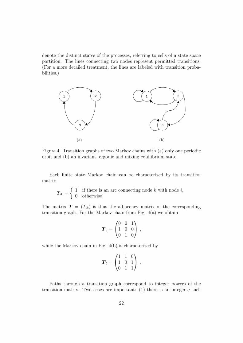
denote the distinct states of the processes, referring to cells of a state spacepartition. The lines connecting two nodes represent permitted transitions.(For a more detailed treatment, the lines are labeled with transition proba-bilities.)

1

3

2

(a)

1

3

2

(b)

Figure 4: Transition graphs of two Markov chains with (a) only one periodicorbit and (b) an invariant, ergodic and mixing equilibrium state.

Each finite state Markov chain can be characterized by its transitionmatrix

Tik =

1 if there is an arc connecting node k with node i,0 otherwise

The matrix T = (Tik) is thus the adjacency matrix of the correspondingtransition graph. For the Markov chain from Fig. 4(a) we obtain

T a =

0 0 11 0 00 1 0

,

while the Markov chain in Fig. 4(b) is characterized by

T b =

1 1 01 0 10 1 1

.

Paths through a transition graph correspond to integer powers of thetransition matrix. Two cases are important: (1) there is an integer q such

22

that T q is a diagonal matrix, and (2) there is an integer q such that T q ispositive. Consider the matrix T q

a with q = 3,

T 3a =

1 0 00 1 00 0 1

,

which is the identity matrix in three-dimensional space. It indicates a closedpath of length three through the graph shown in Fig. 4(a), correspondingto three period-three orbits (distinguished only by their initial conditions)of the Markov chain. Periodic orbits for Markov chains can be related tostationary and ergodic — but not mixing — probability distributions overstate space.

On the other hand, we find that all elements of

T 2b =

2 1 11 2 11 1 2

are positive, such that T 2

b is positive, i.e. contains no zeros. This means thatevery node in the transition graph shown in Fig. 4(b) can be reached fromevery other node through a path of length two, which is not a periodic orbit.The corresponding Markov chain is thus irreducible and aperiodic.

For the normalized transition matrix

N =1

λ1

T ,

where λ1 is the largest eigenvalue of T , one gets by virtue of the FrobeniusPerron theorem a unique eigenstate of N for eigenvalue one, i.e. an invariantequilibrium state (Norris 1998).

Further properties of this equilibrium state are due to the features of thetransition graph. The fact that every state is accessible from every otherstate through a path of sufficient length is known as ergodicity. Moreover,as paths of sufficient length intersect with each other, the system exhibitsdecaying temporal correlations, which is known as the mixing property.

To conclude, two interesting cases for finite state Markov chains can bedistinguished. If an integer power of the transition matrix is diagonal, theMarkov chain possesses invariant and ergodic, but not mixing, equilibrium

23

states. If, on the other hand, an integer power of the transition matrix isstrictly positive, the Markov chain has invariant, ergodic and mixing equi-librium states corresponding to thermal equilibrium states according to theKMS criterion. For more details see the relevant literature, for instance Nor-ris (1998).

Acknowledgements

This work has been supported by an EPSCR Bridging the Gaps grant on Cog-nitive Systems Sciences. Adam Barrett was partly supported by a postdoc-toral fellowship at the Institute for Adaptive and Neural Computation in theSchool of Informatics at the University of Edinburgh, funded by the HumanFrontier Science Program. We thank Slawomir Nasuto and two anonymousreferees for substantial help improving the paper.

References

Allefeld, C., Atmanspacher, H., and Wackermann, J. (2009). Mental statesas macrostates emerging from EEG dynamics. Chaos, 19:015102.

Amari, S.-I. (1974). A method of statistical neurodynamics. Kybernetik,14:201 – 215.

Amari, S.-I. and Maginu, K. (1988). Statistical neurodynamics of associativememory. Neural Networks, 1(1):63 – 73.

Amari, S.-I., Yoshida, K., and Kanatani, K.-I. (1977). A mathematical foun-dation for statistical neurodynamics. SIAM Journal of Applied Mathemat-ics, 33(1):95 – 126.

Anderson, J. A. and Rosenfeld, E., editors (1988). Neurocomputing. Foun-dations of Research, volume 1. MIT Press, Cambridge (MA).

Atmanspacher, H. (2007). Contextual emergence from physics to cognitiveneuroscience. Journal of Consciousness Studies, 14(1/2):18 – 36.

Atmanspacher, H. and beim Graben, P. (2007). Contextual emergenceof mental states from neurodynamics. Chaos and Complexity Letters,2(2/3):151 – 168.

24

Atmanspacher, H. and Rotter, S. (2008). Interpreting neurodynamics: con-cepts and facts. Cognitive Neurodynamics, 2(4):297 – 318.

Batterman, R. (2002). The Devil in the Details. Oxford University Press,Oxford.

Bishop, R. C. and Atmanspacher, H. (2006). Contextual emergence in thedescription of properties. Foundations of Physics, 36(12):1753 – 1777.

Bollobas, B. (2001). Random Graphs, volume 73 of Cambridge Studies inAdvanced Mathematics. Cambridge University Press, Cambridge (UK).

Chalmers, D. J. (2000). What is a neural correlate of consciousness? InMetzinger (2000), pages 17 – 39.

Exel, R. (2004). KMS states for generalized gauge actions on Cuntz-Kriegeralgebras (An application of the Ruelle-Perron-Frobenius theorem). Bul-letin of the Brazilian Mathematical Society, 35(1):1 – 12.

Freeman, W. J. (2007). Definitions of state variables and state space forbrain-computer interface. part 1. multiple hierarchical levels of brain func-tion. Cognitive Neurodynamics, 1:3 – 14.

Gaveau, B. and Schulman, L. S. (2005). Dynamical distance: coarse grains,pattern recognition, and network analysis. Bulletin des Sciences Mathe-matiques, 129:631 – 642.

beim Graben, P. (2004). Incompatible implementations of physical symbolsystems. Mind and Matter, 2(2):29 – 51.

beim Graben, P. (2008). Foundations of neurophysics. In beim Graben, P.,Zhou, C., Thiel, M., and Kurths, J., editors, Lectures in Supercomputa-tional Neuroscience: Dynamics in Complex Brain Networks, pages 3 – 48.Springer, Berlin.

beim Graben, P. and Atmanspacher, H. (2006). Complementarity in classicaldynamical systems. Foundations of Physics, 36(2):291 – 306.

beim Graben, P. and Kurths, J. (2008). Simulating global properties ofelectroencephalograms with minimal random neural networks. Neurocom-puting, 71(4):999 – 1007.

Guckenheimer, J. and Holmes, P. (1983). Nonlinear Oscillations, DynamicalSystems, and Bifurcations of Vector Fields, Springer, New York.

25

Hopfield, J. J. (1982). Neural networks and physical systems with emergentcollective computational abilities. Proceedings of the National Academy ofSciences of the U.S.A., 79(8):2554 – 2558.

Lind, D. and Marcus, B. (1995). An Introduction to Symbolic Dynamics andCoding. Cambridge University Press, Cambridge (UK).

Maass, W., Natschlager, T., and Markram, H. (2002). Real-time computingwithout stable states: A new framework for neural computation based onperturbations. Neural Computation, 14(11):2531 – 2560.

McCulloch, W. S. and Pitts, W. (1943). A logical calculus of ideas immanentin nervous activity. Bulletin of Mathematical Biophysics, 5:115 – 133.Reprinted in J. A. Anderson and E. Rosenfeld (1988), pp. 18ff.

Metzinger, T., editor (2000). Neural Correlates of Consciousness. MIT Press,Cambridge (MA).

Norris, J.R. (1998). Markov Chains. Cambridge University Press, Cambridge.

Olesen, D. and Pedersen, G. K. (1978). Some C∗-dynamical systems with asingle KMS state. Mathematica Scandinavia, 42:111 – 118.

Pinzari, C., Watatani, Y., and Yonetani, K. (2000). KMS states, entropy andthe variational principle in full C∗-dynamical systems. Communications ofMathematical Physics, 213:331 – 379.

Primas, H. (1998). Emergence in exact natural sciences. Acta PolytechnicaScandinavica, Ma-91:83 – 98.

Ruelle, D. (1968). Statistical mechanics of a one-dimensional lattice gas.Communications of Mathematical Physics, 9:267 – 278.

Ruelle, D. (1989). The thermodynamic formalism for expanding maps. Com-munications of Mathematical Physics, 125:239 – 262.

Sewell, G. L. (2002). Quantum Mechanics and its Emergent Macrophysics.Princeton University Press.

Shalizi, C. R. and Moore, C. (2003). What is a macrostate? subjectiveobservations and objective dynamics. arXiv: cond-mat/0303625.

Sinai, Y. G. (1968). Construction of Markov partitions. Functional Analysisand its Applications, 2(3):245 – 253.

26

Smolensky, P. (1988). On the proper treatment of connectionism. Behavioraland Brain Sciences, 11(1):1 – 74.

Smolensky, P. (2006). Harmony in linguistic cognition. Cognitive Science,30:779 – 801.

Touboul, J., Faugeras, O., and Cessac, B. (2008). Mean field analyis of multi-population neural networks with random synaptic weights and stochasticinput. Technical Report 6454, INRIA, Sophia Antipolis.

Wilson, H. R. and Cowan, J. D. (1972). Excitatory and inhibitory interac-tions in localized populations of model neurons. Biophysical Journal, 12:1– 24.

27