Embed Size (px)
Citation preview

SRI KRISHNA COLLEGE OF ENGINEERING AND TECHNOLOGY
KUNIAMUTHUR, COIMBATORE.641 008.
CURRICULUM DEVELOPMENT CELL
CURRICULUM DESIGN FOR M.E. – PED COURSE
SEMESTER 1:
S.NO CATEGORY SUB CODE SUB NAME L T P C MAX
MARKS
1 FCBS 17MM104 Advanced Mathematics for Electrical Engineers 3 2 0 4 100
2 PC 17PE101 Modeling and Analysis of Electrical Machines 3 2 0 4 100
3 PC 17PE102 Analysis of Power Converters 3 2 0 4 100
4 PC 17PE103 Analysis of Inverters 3 0 0 3 100
5 PE 17PE0XX PE - 1 3 0 0 3 100
6 PE 17PE0XX PE - 2 3 0 0 3 100
7 PC Lab 17PE111 Power Electronics Simulation Laboratory 0 0 3 2 100
Total 18 6 3 23 700
Semester 2:
S.NO CATEGORY SUB CODE SUB NAME L T P C MAX
MARKS
1 PC 17PE201 Solid State DC drives 3 2 0 4 100
2 PC 17PE202 Solid State AC drives 3 2 0 4 100
3 PC 17PE203 System Theory 3 2 0 4 100
4 PE 17PE0XX PE - 3 3 0 0 3 100
5 PE 17PE0XX PE - 4 3 0 0 3 100
6 PSC 17PE0ZZ PSC - I 3 0 0 3 100
7 PC Lab 17PE211 Power Electronics and Drives Laboratory 0 0 3 2 100
8 ****** 17PE212 Technical Seminar 0 0 2 1 100
Total 18 6 5 24 800
FCBS - Foundation Compulsory Basic Science
PC - Programme Core
PSC - Programme Soft Core
PE - Programme Elective

Semester 3:
S.N
O
CATEGORY SUB CODE SUB NAME L T P C MAX
MARKS
1 PSC 17PE0ZZ PSC - II 3 0 0 3 100
2 PE 17PE0XX PE – 5 3 0 0 3 100
3 PE 17PE0XX PE - 6 3 0 0 3 100
4 Project 17PE311 Project Work– Phase I / Internship 0 0 12 6 100
5 ****** 17PE312 Comprehensive Viva – Voce (Objective type Test &
Viva (External))
0 0 2 1 100
Total 9 0 14 16 500
Semester 4:
S.NO CATEGORY SUB CODE SUB NAME L T P C MAX
MARKS
1 Project 17PE411 Project Work – Phase II 0 0 24 12 100
Total 0 0 24 12 100
FCBS - Foundation Compulsory Basic Science
PC - Programme Core
PSC - Programme Soft Core
PE - Programme Elective
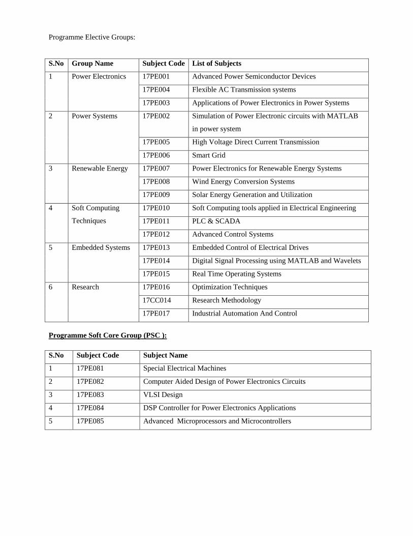
Programme Elective Groups:
S.No Group Name Subject Code List of Subjects
1 Power Electronics 17PE001 Advanced Power Semiconductor Devices
17PE004 Flexible AC Transmission systems
17PE003 Applications of Power Electronics in Power Systems
2 Power Systems 17PE002 Simulation of Power Electronic circuits with MATLAB
in power system
17PE005 High Voltage Direct Current Transmission
17PE006 Smart Grid
3 Renewable Energy 17PE007 Power Electronics for Renewable Energy Systems
17PE008 Wind Energy Conversion Systems
17PE009 Solar Energy Generation and Utilization
4 Soft Computing
Techniques
17PE010 Soft Computing tools applied in Electrical Engineering
17PE011 PLC & SCADA
17PE012 Advanced Control Systems
5 Embedded Systems 17PE013 Embedded Control of Electrical Drives
17PE014 Digital Signal Processing using MATLAB and Wavelets
17PE015 Real Time Operating Systems
6 Research 17PE016 Optimization Techniques
17CC014 Research Methodology
17PE017 Industrial Automation And Control
Programme Soft Core Group (PSC ):
S.No Subject Code Subject Name
1 17PE081 Special Electrical Machines
2 17PE082 Computer Aided Design of Power Electronics Circuits
3 17PE083 VLSI Design
4 17PE084 DSP Controller for Power Electronics Applications
5 17PE085 Advanced Microprocessors and Microcontrollers

Note :
1. Programme Electives (PE) must be framed by having 5 domains, each possessing 3 subjects.
Students should get specialized in any two domains.
2. List of subjects must be given in Programme Soft Core (PSC), so that students can choose
any 2 subjects.
3. Students can earn extra credits by doing certification courses.
Curriculum Structure - Sample
S.No Category Name Actual
Credit Break Up
1 Foundation Compulsory Basic Science
(FCBS)
4
2 Programme Core(PC ) 23
3 Programme Elective(PE) 18
4 Programme Core(PC ) Lab 4
5 Programme Soft Core(PSC ) 6
6 Project 18
7 Comprehensive Viva – Voce 2
Total 75
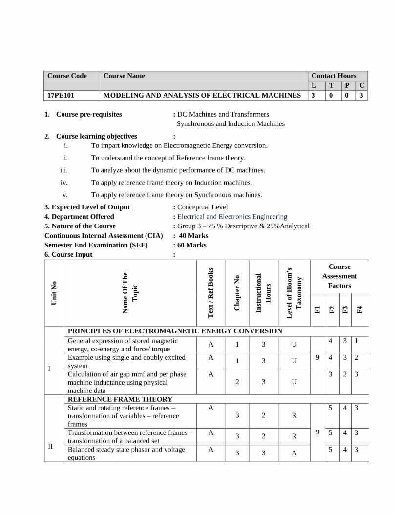
1. Course pre-requisites : DC Machines and Transformers
Synchronous and Induction Machines
2. Course learning objectives :
i. To impart knowledge on Electromagnetic Energy conversion.
ii. To understand the concept of Reference frame theory.
iii. To analyze about the dynamic performance of DC machines.
iv. To apply reference frame theory on Induction machines.
v. To apply reference frame theory on Synchronous machines.
3. Expected Level of Output : Conceptual Level
4. Department Offered : Electrical and Electronics Engineering
5. Nature of the Course : Group 3 – 75 % Descriptive & 25%Analytical
Continuous Internal Assessment (CIA) : 40 Marks
Semester End Examination (SEE) : 60 Marks
6. Course Input :
Un
it N
o
Nam
e O
f T
he
Top
ic
Tex
t /
Ref
Book
s
Ch
ap
ter
No
Inst
ruct
ion
al
Hou
rs
Lev
el o
f B
loom
’s
Taxon
om
y
Course
Assessment
Factors
F1
F2
F3
F4
I
PRINCIPLES OF ELECTROMAGNETIC ENERGY CONVERSION
General expression of stored magnetic
energy, co-energy and force/ torque A 1 3 U
9
4 3 1
Example using single and doubly excited
system
A 1 3 U
4 3 2
Calculation of air gap mmf and per phase
machine inductance using physical
machine data
A 2 3 U
3 2 3
II
REFERENCE FRAME THEORY
Static and rotating reference frames –
transformation of variables – reference
frames
A 3 2 R
9
5 4 3
Transformation between reference frames –
transformation of a balanced set
A 3 2 R
5 4 3
Balanced steady state phasor and voltage
equations
A 3 3 A
5 4 3
Course Code Course Name Contact Hours
L T P C
17PE101 MODELING AND ANALYSIS OF ELECTRICAL MACHINES 3 0 0 3

Variables observed from several frames of
reference
A 3 2 A
5 4 3
III
DC MACHINES
Voltage and toque equations A 10 3 R
9
3 3 2
Dynamic characteristics of permanent
magnet and shunt DC motors
A 10 3 AP
5 4 2
State equations - solution of dynamic
characteristic by Laplace transformation
A 10 3 A
4 4 2
IV
INDUCTION MACHINES
Voltage and toque equations A 6 1 R
9
4 2 1
Transformation for rotor circuits – Voltage
and toque equations in reference frame
variables
A 6 2 AP
4 1 2
Analysis of steady state operation – Free
acceleration characteristics
A 6 2 A
4 1 1
Dynamic performance for load and torque
variations – Dynamic performance for
three phase fault
A 6 3 A
4 1 2
Computer simulation in arbitrary reference
frame
A 6 1 C
5 4 3
V
SYNCHRONOUS MACHINES
Voltage and Torque Equation A 5 1 R
9
5 5 2
Voltage Equation in arbitrary reference
frame and rotor reference frame – Park
equations - Rotor angle
A 5 2 AP 4 4 2
Steady state analysis – Dynamic
performances for torque variations A 5 2 A 3 1 2
Dynamic performance for three phase fault
– Transient stability limit – Critical
clearing time
A 5 3 A 5 5 5
Computer simulation A 5 1 C 5 5 4
Bloom’s Legends:
R-Remembering U-Understanding AP-Applying
A-Analyzing C-Creating E – Evaluating
7. TEXT BOOKS
A. Paul C.Krause, OlegWasyzczuk, Scott S, Sudhoff, “Analysis of Electric Machinery and
Drive Systems”, IEEE Press, Second Edition, 2002
B. Charles Kingsley, A.E. Fitzgerald Jr. and Stephen D. Umans, ‘Electric Machinery’, Tata
McGraw-Hill, Fifth Edition, 2002.
REFERENCE BOOKS
C. R.Krishnan, “Electric Motor Drives, Modeling, Analysis and Control” , Prentice Hall of
India, 2002
D. Samuel Seely, “Electromechanical Energy Conversion”, Tata McGraw Hill Publishing
Company, 1962.
WEB RESOURCES

8. Assessing Level of Bloom’s Taxonomy in Numbers:
R U AP A E C TOTAL
UNIT I 3 3
UNIT II 2 2 4
UNIT III 1 1 1 3
UNIT IV 1 1 2 1 5
UNIT V 1 1 2 1 5
TOTAL 20
9. Weightage of Bloom’s Taxonomy in the Syllabus
R U AP A E C TOTAL
( %)
UNIT I 0 15 0 0 0 0 15
UNIT II 10 0 0 10 0 0 20
UNIT III 5 0 5 5 0 0 15
UNIT IV 5 0 5 10 0 5 25
UNIT V 5 0 5 10 0 5 25
TOTAL 25 15 15 35 0 10 100
Lower Order Thinking (%) 55%
Higher Order Thinking (%) 45%
10. Expected outcome of the course:
Upon successful completion of this course, the student will be able to:
CO1: know about Electromagnetic Energy conversion
CO2: understand the concept of Reference frame theory
CO3: analyze about DC machines with dynamic performance
CO4: apply reference frame theory on Induction machines.
CO5: apply reference frame theory on Synchronous machines.
11. Mapping course outcome with Bloom’s Taxonomy LOT and HOT:
R U AP A E C
CO1 √ √ √
CO2 √ √ √
CO3 √ √ √
CO4 √ √ √ √
CO5 √ √ √ √

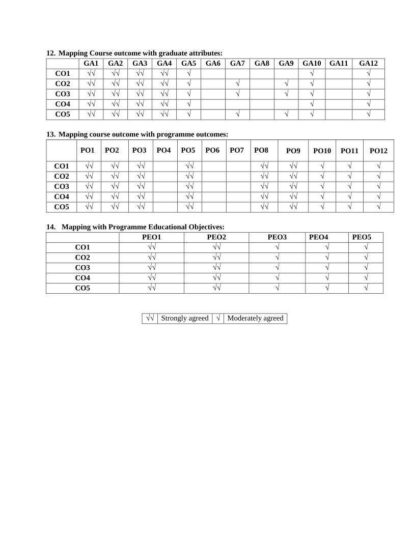
12. Mapping Course outcome with graduate attributes:
GA1 GA2 GA3 GA4 GA5 GA6 GA7 GA8 GA9 GA10 GA11 GA12
CO1 √√ √√ √ √ √
CO2 √√ √√ √√ √ √ √ √ √ √
CO3 √√ √ √ √ √ √√ √
CO4 √√ √√ √ √√ √√ √√ √√
CO5 √√ √√ √√ √√ √√
13. Mapping course outcome with programme outcomes:
PO1 PO2 PO3 PO4 PO5 PO6 PO7 PO8 PO9 PO10 PO11 PO12
CO1 √√ √√ √ √ √ √ √ √ √ √
CO2 √√ √ √ √ √ √ √ √ √
CO3 √√ √ √ √ √ √ √ √
CO4 √√ √ √ √ √
CO5 √√ √ √ √ √ √ √
14. Mapping with Programme Educational Objectives:
PEO1 PEO2 PEO3 PEO4 PEO5
CO1 √√ √ √ √
CO2 √√ √ √ √
CO3 √
CO4 √ √ √ √
CO5 √√ √ √ √
√√ Strongly agreed √ Moderately agreed

1. Course pre-requisites : Power Electronics
2. Course learning objectives :
i. To provide the electrical circuit concepts behind the different working modes of power
Converters.
ii. To equip with required skills to derive the criteria for the design of power converters starting
from basic fundamentals.
iii. To analyze and comprehend the various operating modes of different configurations of
Power converters.
iv. To design different power converters namely AC to DC, DC to DC and AC to AC converters.
3. Expected Level of Output : Analysis Level
4. Department Offered : Electrical and Electronics Engineering
5. Nature of the Course : Group 3 –50% Descriptive & 50%Analytical
Continuous Internal Assessment (CIA) : 40 Marks
Semester End Examination (SEE) : 60 Marks
6. Course Input :
Un
it N
o
Nam
e O
f T
he
Top
ic
Tex
t /
Ref
Book
s
Ch
ap
ter
No
Inst
ruct
ion
al
Hou
rs
Lev
el o
f B
loom
’s
Taxon
om
y
Course
Assessment
Factors
F1
F2
F3
F4
I
SINGLE PHASE RECTIFIER
Static Characteristics of power diode, SCR
and GTO,Half controlled and fully
controlled converters with R-L, R-L-E
loads and free wheeling diodes
A 2 & 5 5 U,A,Ap
9
5 4 4
Continuous and discontinuous
modes of operation - inverter operation F 6 U,A 5 4 4
Sequence control of converters –
performance
parameters: harmonics, ripple, distortion,
power factor
F 3 1 U,A 5 4 4
Effect of source impedance and
overlap-reactive power and power balance
in converter circuits
F 6 3 U,A 5 4 4
THREE PHASE RECTIFIER
Course Code Course Name Contact Hours
L T P C
17PE102 ANALYSIS OF POWER CONVERTER 3 0 0 3

II
Semi and fully controlled converter with R,
R-L, R-L-E - loads and free wheeling
diodes
A,F 5,6 5 U,A,Ap
9
5 4 4
Inverter operation and its limit –
performance parameters F 6 2 U,A 5 4 4
Effect of source impedance and over
lap – 12 pulse converter F 6 2 U,A 5 4 4
III
DC-DC CONVERTERS
Principles of step-down and step-up
converters B,F 8,7 1 U
9
5 4 4
Analysis of buck, boost, buck-boost
converters B,F 8,7 3 A,Ap 5 4 4
Cuk Converters B,F 8,7 2 A,Ap 5 4 4
Time ratio and current limit control- Full
bridge converter B,F 8,7 1 U 5 4 4
Resonant converters A,B 9,12 1 U,A,Ap 5 4 4
Quasi resonant converters
A,B 9,12 1 U,A,Ap 5 4 4
IV
AC VOLTAGE CONTROLLERS
Static Characteristics of TRIAC B,F 11,9 1 U,A
9
5 4 4
Principle of phase control: single phase
controllers B,F 11,9 2 U,Ap 5 4 4
Three phase controllers B,F 11,9 2 U,Ap 5 4 4
Various configurations B,F 11,9 2 U 5 4 4
Analysis with R and R-L loads B,F 11,9 2 A 5 4 4
V
CYCLOCONVERTERS
Principle of operation – Single phase Dual
converters B,F 10,10 1 U,A,Ap
9
5 4 4
Three-phase Dual converters B,F 11,9 1 U,A,Ap 5 4 4
Single phase Cyclo-Converters B,F 11,9 2 U,A,Ap 5 4 4
Three phase Cyclo-Converters B,F 11,9 2 U,A,Ap 5 4 4
Power factor Control F 13 1 U,A 5 4 4
Introduction to Matrix converters 2 U 5 4 4
Bloom’s Legends:
R-Remembering U-Understanding AP-Applying
A-Analyzing C-Creating E – Evaluating
7. TEXT BOOKS
A. Ned Mohan,T.M Undeland and W.P Robbin, “Power Electronics: converters, Application
and design” Wiley India edition, 2006.
B. M.D.Sungh and K.B.Kanchandani,”Power Electronics”, Tata McgGraw Hill,2012
REFERENCE BOOKS
C. Rashid M.H., “Power Electronics Circuits, Devices and Applications ", Pierson Prentice
Hall India, New Delhi, 2010.
D. E. P.C Sen.," Modern Power Electronics ", Wheeler publishing Co, First Edition,

New Delhi-1998.
E. P.S.Bimbra, “Power Electronics”, Khanna Publishers, Fourth Edition, 2012.
F. Power Electronics by Vedam Subramanyam, New Age International publishers, New Delhi
Second Edition, 2006
WEB RESOURCES
http://www.nptel.ac.in/courses/Webcourse-contents/IITKharagpur/Power Electronics/PDF
8. Assessing Level of Bloom’s Taxonomy in Numbers:
R U AP A E C TOTAL
UNIT I 0 4 1 4 0 0 9
UNIT II 0 3 1 3 0 0 7
UNIT III 0 4 4 4 0 0 12
UNIT IV 0 4 2 2 0 0 8
UNIT V 0 6 4 5 0 0 15
TOTAL 51
9. Weightage of Bloom’s Taxonomy in the Syllabus
R U AP A E C TOTAL
( %)
UNIT I 0 7.84 1.96 7.84 0 0 17.64
UNIT II 0 5.88 1.96 5.88 0 0 13.72
UNIT III 0 7.84 7.84 7.84 0 0 23.52
UNIT IV 0 7.84 3.92 3.92 0 0 15.68
UNIT V 0 11.76 7.84 8.20 0 0 27.8
TOTAL 0 41.16 23.52 33.68 0 0 98.36
Lower Order Thinking (%) 64.68 %
Higher Order Thinking (%) 33.68%
10. Expected outcome of the course:
Upon successful completion of this course, the student will be able to:
CO1: Know static and dynamic characteristics of power electronic devices
CO2: Analyze the RMS, Average values of output voltage and current of the single and three phase
rectifiers and they can also be able to calculate performance parameters
CO3: Analyze DC Chopper operation
CO4: Analyze AC Voltage controller operation
CO5: Analyze Cyclo converters operation
11. Mapping course outcome with Bloom’s Taxonomy LOT and HOT:
R U AP A E C
CO1 √ √ √
CO2 √ √ √
CO3 √ √ √
CO4 √ √ √
CO5 √ √ √
12. Mapping Course outcome with graduate attributes:
GA1 GA2 GA3 GA4 GA5 GA6 GA7 GA8 GA9 GA10 GA11 GA12
CO1 √√ √√ √√ √√ √ √ √
CO2 √√ √√ √√ √√ √ √ √ √ √
CO3 √√ √√ √√ √√ √ √ √ √ √
CO4 √√ √√ √√ √√ √ √ √
CO5 √√ √√ √√ √√ √ √ √ √ √
13. Mapping course outcome with programme outcomes:
PO1 PO2 PO3 PO4 PO5 PO6 PO7 PO8 PO9 PO10 PO11 PO12
CO1 √√ √√ √√ √√ √√ √√ √ √ √
CO2 √√ √√ √√ √√ √√ √√ √ √ √
CO3 √√ √√ √√ √√ √√ √√ √ √ √
CO4 √√ √√ √√ √√ √√ √√ √ √ √
CO5 √√ √√ √√ √√ √√ √√ √ √ √
14. Mapping with Programme Educational Objectives:
PEO1 PEO2 PEO3 PEO4 PEO5
CO1 √√ √√ √ √ √
CO2 √√ √√ √ √ √
CO3 √√ √√ √ √ √
CO4 √√ √√ √ √ √
CO5 √√ √√ √ √ √
√√ Strongly agreed √ Moderately agreed

1. Course pre-requisites : Power Electronics
2. Course learning objectives :
i. To provide the electrical circuit concepts behind the different working modes of inverters so as
to enable deep understanding of their operation.
ii. To equip with required skills to derive the criteria for the design of power converters for UPS
Drives etc.,
iii. To study the working of advanced types of inverters such as multilevel inverters and resonant
inverters.
iv. Ability to analyze and comprehend the various operating modes of different configurations of
power converters.
v. Ability to design different single phase and three phase inverters.
3. Expected Level of Output : Conceptual Level
4. Department Offered : Electrical &Electronics Engineering
5. Nature of the Course : Group 1 – 100 % Descriptive
Continuous Internal Assessment (CIA) : 40 Marks
Semester End Examination (SEE) : 60 Marks
6. Course Input :
Un
it N
o
Nam
e O
f T
he
Top
ic
Tex
t /
Ref
Book
s
Ch
ap
ter
No
Inst
ruct
ion
al
Hou
rs
Lev
el o
f B
loom
’s
Taxon
om
y
Course
Assessment
Factors
F1
F2
F3
F4
I
SINGLE PHASE INVERTERS
Introduction to self commutated switches :
MOSFET and IGBT - Principle of
operation of half and full bridge inverters
A 6 4 U
12
5 5 4
Performance parameters –Voltage control
of single phase inverters using various
PWM techniques
A 6 3 U,C 5 5 4
Various harmonic elimination techniques A 6 2 R,U 5 4 3
Forced commutated Thyristor inverters-
Design of UPS A 6,10 3 U,AP,C 5 4 3
THREE PHASE VOLTAGE SOURCE INVERTERS
Course Code Course Name Contact Hours
L T P C
17PE103 ANALYSIS OF INVERTERS 3 0 0 3

II
180 degree and 120 degree conduction
mode inverters with star and delta
connected loads
A 6 3 R,U,A
9
5 4 3
Voltage control of three phase inverters A 6 2 U 5 4 3
Single, multi pulse, sinusoidal, space
vector modulation techniques A,E 6,8 2 U,A 5 5 4
Application to drive system A 6 2 R,U 5 5 5
III
CURRENT SOURCE INVERTERS
Operation of six-step thyristor inverter –
Inverter operation modes E 8 3 R,U,C
9
5 5 3
Load – Commutated inverters – Auto
Sequential Current Source Inverter (ASCI) E 8 1 R,U 5 4 3
Current pulsations – Comparison of current
source inverter and voltage source inverters A 6 2 R,U 5 5 3
PWM techniques for current source
inverters. A 6 3 R,U,AP 5 4 4
IV
MULTILEVEL & BOOST INVERTERS
Multilevel concept – Diode clamped –
Flying capacitor – Cascade type multilevel
inverters
A 9 3 R,U,A
9
5 5 3
Comparison of multilevel inverters
application of multilevel inverters A 9 2 R,U,A 5 4 5
PWM techniques for MLI A 6 2 R,U,A 5 5 3
Boost Inverter-Basic Principle A 6 2 R,U,C 5 5 3
V
RESONANT INVERTERS
Series and parallel resonant inverters -
Voltage control of resonant inverters A 11 2 R,U,C
6
5 5 3
Class E resonant inverter A 11 2 R,U 5 4 3
Resonant DC – link inverters. A 11 2 R,U 5 4 2
Bloom’s Legends:
R-Remembering U-Understanding AP-Applying
A-Analyzing C-Creating E – Evaluating
7. TEXT BOOKS
A. Rashid M.H., "Power Electronics Circuits, Devices and Applications", Prentice Hall India, Third
Edition, New Delhi, 2013.
B. Bimal K.Bose “Modern Power Electronics and AC Drives”, Pearson Education,2006
REFERENCE BOOKS
C. Ned Mohan, Undeland and Robbin, “Power Electronics: converters, Application and design”, John
Wiley and sons.Inc, Newyork, Reprint 2009
D. Jai P.Agrawal, “Power Electronics Systems”, Pearson Education, Second Edition, 2002.
E. P.S.Bimbra, “Power Electronics”, Khanna Publishers, Eleventh Edition, 2012
WEB RESOURCES
http://www.nptel.ac.in/courses/Webcourse-contents/IITKharagpur/Power
Electronics/PDF
8. Assessing Level of Bloom’s Taxonomy in Numbers:
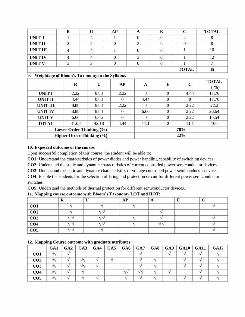
R U AP A E C TOTAL
UNIT I 1 4 1 0 0 2 8
UNIT II 2 4 0 2 0 0 8
UNIT III 4 4 1 0 0 1 10
UNIT IV 4 4 0 3 0 1 12
UNIT V 3 3 0 0 0 1 7
TOTAL 45
9. Weightage of Bloom’s Taxonomy in the Syllabus
R U AP A E C TOTAL
( %)
UNIT I 2.22 8.88 2.22 0 0 4.44 17.76
UNIT II 4.44 8.88 0 4.44 0 0 17.76
UNIT III 8.88 8.88 2.22 0 0 2.22 22.2
UNIT IV 8.88 8.88 0 6.66 0 2.22 26.64
UNIT V 6.66 6.66 0 0 0 2.22 15.54
TOTAL 31.08 42.18 4.44 11.1 0 11.1 100
Lower Order Thinking (%) 78%
Higher Order Thinking (%) 22%
10. Expected outcome of the course:
Upon successful completion of this course, the student will be able to:
CO1: Understand the characteristics of power diodes and power handling capability of switching devices
CO2: Understand the static and dynamic characteristics of current controlled power semiconductor devices
CO3: Understand the static and dynamic characteristics of voltage controlled power semiconductor devices
CO4: Enable the students for the selection of firing and protection circuit for different power semiconductor
switches
CO5: Understand the methods of thermal protection for different semiconductor devices.
11. Mapping course outcome with Bloom’s Taxonomy LOT and HOT:
R U AP A E C
CO1 √ √ √ √
CO2 √ √ √ √
CO3 √ √ √ √ √ √ √
CO4 √ √ √ √ √ √ √ √
CO5 √ √ √ √
12. Mapping Course outcome with graduate attributes:
GA1 GA2 GA3 GA4 GA5 GA6 GA7 GA8 GA9 GA10 GA11 GA12
CO1 √√ √ √ √ √ √ √
CO2 √√ √ √√ √ √ √ √ √ √ √
CO3 √√ √ √√ √ √ √ √ √ √
CO4 √√ √ √ √√ √√ √ √ √ √
CO5 √√ √ √ √ √ √ √ √ √ √

13. Mapping course outcome with programme outcomes:
PO1 PO2 PO3 PO4 PO5 PO6 PO7 PO8 PO9 PO10 PO11 PO12
CO1 √√ √√ √ √ √ √ √ √ √
CO2 √√ √√ √ √ √ √ √ √ √
CO3 √√ √√ √ √ √ √ √ √ √
CO4 √√ √√ √ √ √ √ √ √ √
CO5 √√ √√ √ √ √ √ √ √
14. Mapping with Programme Educational Objectives:
PEO1 PEO2 PEO3 PEO4 PEO5
CO1 √√ √ √ √
CO2 √√ √
CO3 √√ √
CO4 √√ √ √ √
CO5 √√ √
√√ Strongly agreed √ Moderately agreed
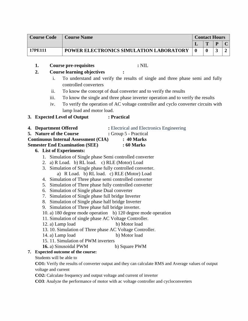
1. Course pre-requisites : NIL
2. Course learning objectives :
i. To understand and verify the results of single and three phase semi and fully
controlled converters
ii. To know the concept of dual converter and to verify the results
iii. To know the single and three phase inverter operation and to verify the results
iv. To verify the operation of AC voltage controller and cyclo converter circuits with
lamp load and motor load.
3. Expected Level of Output : Practical
4. Department Offered : Electrical and Electronics Engineering
5. Nature of the Course : Group 5 - Practical
Continuous Internal Assessment (CIA) : 40 Marks
Semester End Examination (SEE) : 60 Marks
6. List of Experiments:
1. Simulation of Single phase Semi controlled converter
2. a) R Load. b) RL load. c) RLE (Motor) Load
3. Simulation of Single phase fully controlled converter.
a) R Load. b) RL load. c) RLE (Motor) Load
4. Simulation of Three phase semi controlled converter
5. Simulation of Three phase fully controlled converter
6. Simulation of Single phase Dual converter
7. Simulation of Single phase full bridge Inverter
8. Simulation of Single phase half bridge Inverter
9. Simulation of Three phase full bridge inverter.
10. a) 180 degree mode operation b) 120 degree mode operation
11. Simulation of single phase AC Voltage Controller.
12. a) Lamp load b) Motor load
13. 10. Simulation of Three phase AC Voltage Controller.
14. a) Lamp load b) Motor load
15. 11. Simulation of PWM inverters
16. a) Sinusoidal PWM b) Square PWM 7. Expected outcome of the course:
Students will be able to
CO1: Verify the results of converter output and they can calculate RMS and Average values of output
voltage and current
CO2: Calculate frequency and output voltage and current of inverter
CO3: Analyze the performance of motor with ac voltage controller and cycloconverters
Course Code Course Name Contact Hours
L T P C
17PE111 POWER ELECTRONICS SIMULATION LABORATORY 0 0 3 2

1. Course pre-requisites : Power Electronics, DC machines, Analysis of Power
Converters, Control Systems
2. Course learning objectives :
i. To study the fundamentals of motors and mechanical systems
ii. To study about converter control of DC motor drive
iii. To study about chopper control of DC motor drive
iv. To study about closed loop control of DC motor drive
v. To Study about Digital control of DC motor drive
3. Expected Level of Output : Conceptual Level
4. Department Offered : Electrical and Electronics Engineering
5. Nature of the Course : Group 3 – 60% Descriptive & 40%Analytical
Continuous Internal Assessment (CIA) : 40 Marks
Semester End Examination (SEE) : 60 Marks
6. Course Input :
Un
it N
o
Nam
e O
f T
he
Top
ic
Tex
t /
Ref
Book
s
Ch
ap
ter
No
Inst
ruct
ion
al
Hou
rs
Lev
el o
f B
loom
’s
Taxon
om
y
Course
Assessment
Factors
F1
F2
F3
F4
I
DC MOTORS FUNDAMENTALS AND MECHANICAL SYSTEMS
DC motor- Types, Induced emf, speed-
torque relations A 2
1 R
9
4 4 2
Speed control- Ward Leonard control ,
Constant torque and constant horse power
operation
A 2 1
R 5 5 3
Introduction to high speed drives and
modern drives, Characteristics of
mechanical system, Dynamic equations
A 1 2
U 5 5 3
Components of torque, types of load ,
Requirements of drives characteristics
A 2 2 R 5 5 3
Multi-quadrant operation; Drive elements A 2 2 U 5 5 3
Types of motor duty and selection of motor
rating
A 2 1 U 5 5 3
CONVERTER CONTROL
Course Code Course Name Contact Hours
L T P C
17PE201 SOLID STATE DC DRIVES 3 0 0 3

II
Principle of phase control – Fundamental
relations
A 3
1 AP
9
4 4 2
Analysis of series and separately excited
DC motor with single-phase converters
A 3 2 A 3 3 3
Analysis of series and separately excited
DC motor with three phase converter
A 3 2 A 5 5 4
Performance characteristics - Continuous
and discontinuous armature current
operations
A 3 1 A
4 4 3
Current ripple and its effect on
performance, Operation with freewheeling
diode
A 3 1 A
5 4 4
Implementation of braking schemes A 3 1 AP 3 3 3
Drive employing dual converter A 3 1 AP 4 3 2
III
CHOPPER CONTROL
Introduction to time ratio control and
frequency modulation
A 4 1 AP
9
5 4 3
Class A, B chopper controlled DC motor
performance analysis
A 4
1 A 5 4 4
Class C, D chopper controlled DC motor
performance analysis
A 4
2 A 5 4 4
Class E chopper controlled DC motor
performance analysis - multi-quadrant
control
A 4 2 A
4 3 3
Chopper based implementation of braking
schemes
A 4
2 A 3 3 3
Multi-phase chopper A 4
1 U
IV
CLOSED LOOP CONTROL
Modeling of drive elements – Equivalent
circuit
A 2 1 R
9
3 3 3
Transfer function of self, separately excited
DC motors
A 2
2 E 4 3 3
Linear Transfer function model of power
converters
A 2
1 E 5 4 3
Transfer function of Sensing and feedback
elements
A 2
1 E 5 5 5
Closed loop speed control – Current and
speed loops
A 5
1 AP 5 4 4
P, PI and PID controllers – Response
comparison
A 5
2 AP 5 4 4
Simulation of converter and chopper fed
DC drive
B 4
1 C 5 4 4
DIGITAL CONTROL OF DC DRIVE

V
Phase Locked Loop control B 3 1 A
9
4 4 4
Micro-computer control of DC drives E 5
2 AP 5 4 4
Program flow chart for constant horse
power
B 4
2 E 4 3 2
Load disturbed operations B 4 2 A 5 4 4
Speed detection and gate firing A 5
2 U 5 4 4
Bloom’s Legends:
R-Remembering U-Understanding AP-Applying
A-Analyzing C-Creating E – Evaluating
7. TEXT BOOKS
A. Gopal K Dubey, “Power Semiconductor controlled Drives”, Prentice Hall Inc, NewYersy 1989.
B. R.Krishnan, “Electric Motor Drives – Modeling, Analysis and Control”, Prentice-Hall of India
Pvt. Ltd., New Delhi, 2003.
REFERENCE BOOKS
C. Gobal K.Dubey, “Fundamentals of Electrical Drives”, Alpha Science International, II Edition,
2002.
D. Bimal K.Bose “Modern Power Electronics and AC Drives”, Pearson Education (Singapore)
Ltd., New Delhi, 2003.
E. Vedam Subramanyam, “Electric Drives – Concepts and Applications”, Tata McGraw-Hill
publishing company Ltd., New Delhi, 2002.
WEB RESOURCES
8. Assessing Level of Bloom’s Taxonomy in Numbers:
R U AP A E C TOTAL
UNIT I 3 3 0 0 0 0 6
UNIT II 0 0 3 4 0 0 7
UNIT III 0 1 1 4 0 0 6
UNIT IV 1 0 2 0 3 1 7
UNIT V 0 1 1 2 1 0 5
TOTAL 31
9. Weight age of Bloom’s Taxonomy in the Syllabus:
R U AP A E C TOTAL
( %)
UNIT I 9.67 9.67 0 0 0 0 19.35
UNIT II 0 0 9.67 12.9 0 0 22.58
UNIT III 0 3.22 3.22 12.9 0 0 19.35
UNIT IV 3.22 0 6.45 0 9.67 3.22 22.58
UNIT V 0 3.22 3.22 6.45 3.22 0 16.13
TOTAL 12.89 16.11 22.56 32.25 12.89 3.22 99.99
Lower Order Thinking (%) 51.56%
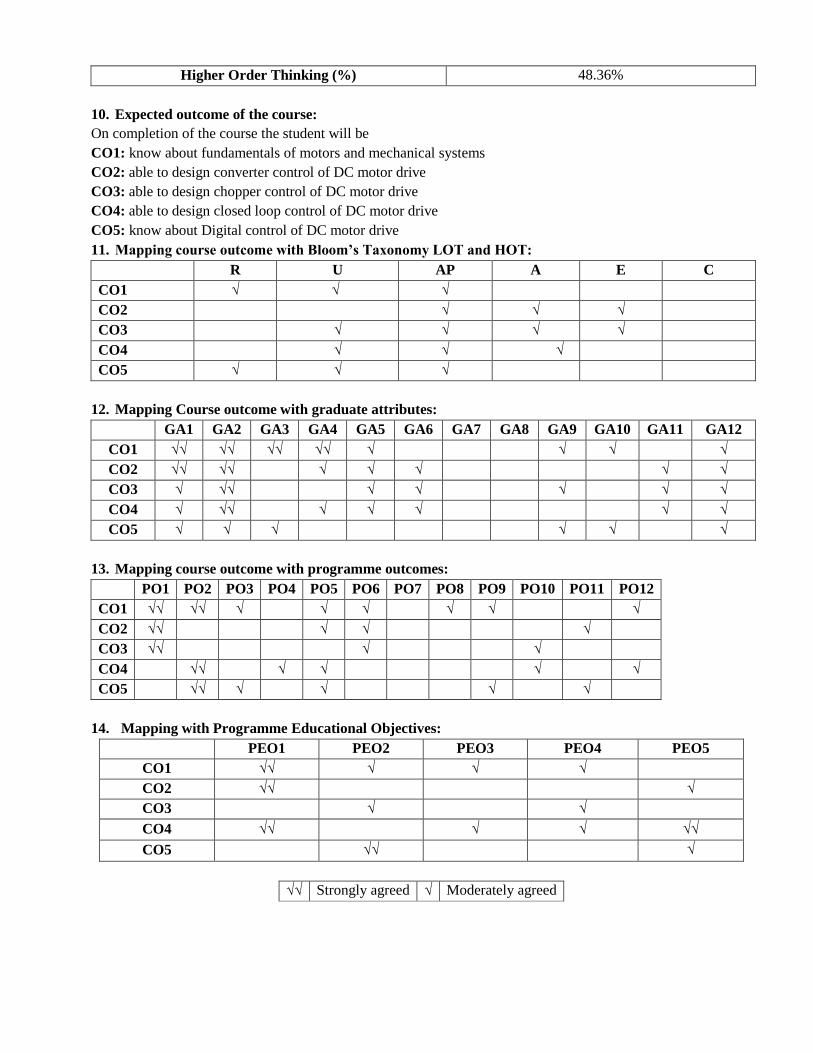
Higher Order Thinking (%) 48.36%
10. Expected outcome of the course:
On completion of the course the student will be
CO1: know about fundamentals of motors and mechanical systems
CO2: able to design converter control of DC motor drive
CO3: able to design chopper control of DC motor drive
CO4: able to design closed loop control of DC motor drive
CO5: know about Digital control of DC motor drive
11. Mapping course outcome with Bloom’s Taxonomy LOT and HOT:
R U AP A E C
CO1 √ √ √
CO2 √ √ √
CO3 √ √ √ √
CO4 √ √ √
CO5 √ √ √
12. Mapping Course outcome with graduate attributes:
GA1 GA2 GA3 GA4 GA5 GA6 GA7 GA8 GA9 GA10 GA11 GA12
CO1 √√ √√ √√ √√ √ √ √ √
CO2 √√ √√ √ √ √ √ √
CO3 √ √√ √ √ √ √ √
CO4 √ √√ √ √ √ √ √
CO5 √ √ √ √ √ √
13. Mapping course outcome with programme outcomes:
PO1 PO2 PO3 PO4 PO5 PO6 PO7 PO8 PO9 PO10 PO11 PO12
CO1 √√ √√ √ √ √ √ √ √
CO2 √√ √ √ √
CO3 √√ √ √
CO4 √√ √ √ √ √
CO5 √√ √ √ √ √
14. Mapping with Programme Educational Objectives:
PEO1 PEO2 PEO3 PEO4 PEO5
CO1 √√ √ √ √
CO2 √√ √
CO3 √ √
CO4 √√ √ √ √√
CO5 √√ √
√√ Strongly agreed √ Moderately agreed

1. Course pre-requisites : Ac Machines, Power Electronics ,Analysis of power
Converter, Control system
2. Course learning objectives :
i. To understand various operating regions of the induction motor drives.
ii. To study and analyze the operation of VSI & CSI fed induction motor control.
iii. To understand the speed control of induction motor drive from the rotor side.
iv. To understand the field oriented control of induction machine.
v. To understand the control of synchronous motor drives.
3. Expected Level of Output : Conceptual Level
4. Department Offered :EEE
5. Nature of the Course : C. Group 3 :70% Descriptive & 30%Analytical
Continuous Internal Assessment (CIA) : 40 Marks
Semester End Examination (SEE) : 60 Marks
6. Course Input :
Un
it N
o
Nam
e O
f T
he
Top
ic
Tex
t /
Ref
Book
s
Ch
ap
ter
No
Inst
ruct
ion
al
Hou
rs
Lev
el o
f B
loom
’s
Taxon
om
y
Course
Assessment
Factors
F1
F2
F3
F4
I
INTRODUCTION TO INDUCTION MOTORS
Steady state performance equations –
Rotating magnetic field – Torque
production, Equivalent circuit
A 6 3 R,A
9
4 4 4
Variable voltage, constant frequency
operation – Variable frequency operation,
constant Volt/Hz operation
A 6 3 U, C 4 4 5
Drive operating regions, variable stator
current operation, different braking
methods.
A 6 3 U,A 4 4 4
VSI AND CSI FED INDUCTION MOTOR DRIVES
AC voltage controller circuit A 6 1 U,A
9
5 4 4
Step inverter voltage control A 6 2 R,A 5 4 4
Closed loop variable frequency PWM A 6 3 U,A 5 4 5
Course Code Course Name Contact Hours
L T P C
17PFK202 SOLID STATE AC DRIVES 3 1 0 4

II
inverter with dynamic braking
CSI fed IM variable frequency drives
comparison A 6 3 R,A 4 3 4
III
ROTOR CONTROLLED INDUCTION MOTOR DRIVES
Static rotor resistance control A 6 2 U,A
4 4 4
Injection of voltage in the rotor circuit A 6 2 U,A 3 4 4
Static scherbius drive A 6 2 A 4 3 5
Power factor considerations – Modified
Kramer drives A 6 3 Ap,A 4 4 5
IV
VECTOR CONTROLLED INDUCTION MOTOR DRIVES
Field oriented control of induction
machines – Theory D 8 2 U,A
9
4 3 4
DC drive analogy – Direct and Indirect
methods – Flux vector estimation D 8 2 B,A 4 4 4
Direct torque control of Induction
Machines D 8 2 E,Ap 4 4 5
Torque expression with stator and rotor
fluxes, DTC control strategy D 8 3 U,A 4 3 5
V
SYNCHRONOUS MOTOR DRIVES
Wound field cylindrical rotor motor A 7 2 U,C
4 3 4
Equivalent circuits – Performance
equations of operation from a voltage
source
A 7 3 U,A 4 4 4
Power factor control and V curves A 7 1 U,A 3 4 5
Starting and braking, self control – Load
commutated Synchronous motor drives A 7 2 U,A 4 3 5
Brush and Brushless excitation A 7 1 U,A 4 4 4
Bloom’s Legends:
R-Remembering U-Understanding AP-Applying
A-Analyzing C-Creating E – Evaluating
7. TEXT BOOKS
A. Gobat. K.Dubey, “Fundamentals of Electrical Drives”, Alpha Science International, II Edition,
2002.
B. R.Krishnan, “Electric Motor Drives – Modeling, Analysis and Control”, Prentice-Hall of India Pvt.
Ltd., New Delhi, 2003
REFERENCE BOOKS
C. W.Leonhard, “Control of Electrical Drives”, Narosa Publishing House, 1992.
D. Bimal K.Bose “Modern Power Electronics and AC Drives”, Pearson Education (Singapore) Ltd.,
New Delhi, 2003
E.Vedam Subramanyam, “Electric Drives – Concepts and Applications”, Tata McGraw Hill, 1994.
WEB RESOURCES
B. Assessing Level of Bloom’s Taxonomy in Numbers:

R U AP A E C TOTAL
UNIT I 1 2 0 2 0 0 5
UNIT II 2 1 0 4 0 0 7
UNIT III 0 2 1 4 0 0 7
UNIT IV 0 2 1 3 1 0 7
UNIT V 0 5 0 4 0 1 10
TOTAL 36
C. Weight age of Bloom’s Taxonomy in the Syllabus
R U AP A E C TOTAL
( %)
UNIT I 2.7 5.5 0 5.5 0 0 13.7
UNIT II 5.5 2.7 0 11.1 0 0 19.3
UNIT III 0 5.5 2.7 11.1 0 0 19.3
UNIT IV 0 5.5 2.7 8.3 2.7 0 19.3
UNIT V 0 13.8 0 11.1 0 2.7 27.6
TOTAL
Lower Order Thinking (%) 100 %
Higher Order Thinking (%) NIL
D. Expected outcome of the course:
Upon successful completion of this course, the student will be:
CO1: able to understand various operating regions of the induction motor drives.
CO2: able to study and analyze the operation of VSI & CSI fed induction motor control.
CO3: able to understand the speed control of induction motor drive from the rotor side.
CO4: able to understand the field oriented control of induction machine.
CO5: able to understand the control of synchronous motor drives.
E. Mapping course outcome with Bloom’s Taxonomy LOT and HOT:
R U AP A E C
CO1 √ √√ √
CO2 √√ √ √√
CO3 √ √ √√
CO4 √ √ √√ √
CO5 √√ √√ √
F. Mapping Course outcome with graduate attributes:
GA1 GA2 GA3 GA4 GA5 GA6 GA7 GA8 GA9 GA10 GA11 GA12
CO1 √√ √ √ √ √√
CO2 √√ √√ √ √ √ √ √ √
CO3 √√ √√ √ √ √ √ √
CO4 √√ √√ √ √ √ √ √ √
CO5 √√ √√ √ √ √ √ √ √

G. Mapping course outcome with programme outcomes:
PO1 PO2 PO3 PO4 PO5 PO6 PO7 PO8 PO9 PO10 PO11 PO12
CO1 √√ √√ √ √ √ √ √ √
CO2 √√ √ √ √
CO3 √√ √ √
CO4 √√ √ √ √ √
CO5 √√ √ √ √ √
H. Mapping with Programme Educational Objectives:
PEO1 PEO2 PEO3 PEO4 PEO5
CO1 √√ √ √ √
CO2 √√ √
CO3 √ √
CO4 √√ √ √ √√
CO5 √√ √
√√ Strongly agreed √ Moderately agreed

1. Course pre-requisites :Control Systems
2. Course learning objectives :
i. To understand the basic concepts of state variable representation.
ii. To understand the concepts of discrete time state model.
iii. To acquire the knowledge about controllability and observability
iv. To analyze the stability of linear and non linear systems.
v. To understand the concepts of model control
3. Expected Level of Output : Conceptual Level
4. Department Offered : Electrical and Electronics Engineering
5. Nature of the Course : Group 2 – 100% Analytical
Continuous Internal Assessment (CIA) : 40 Marks
Semester End Examination (SEE) : 60 Marks
6. Course Input :
Un
it N
o
Nam
e O
f T
he
Top
ic
Tex
t /
Ref
Book
s
Ch
ap
ter
No
Inst
ruct
ion
al
Hou
rs
Lev
el o
f
Blo
om
’s
Taxon
om
y Course
Assessment
Factors
F1
F2
F3
F4
I
STATE VARIABLE REPRESENTATION
Introduction-Concept of State-State equation
for Dynamic Systems A 2 3 U
12
5 5 2
Time invariance and linearity-No uniqueness
of state model-State Diagrams A 2 2 AP 5 5 0
Physical System and State Assignment -
Solution of State Equation A 3 2 A 5 5 1
Existence and uniqueness of solutions to
Continuous-time state equations- Evaluation
of matrix exponential
A 3 2 E 5 4 1
System modes-Role of Eigen values and
Eigenvectors A 4 3 R 5 3 0
II
DISCRETE TIME STATE MODEL
Introduction – Discrete Time State Model A 5 3 U
12
5 2 0
Sample and Hold Digital Equivalent –
Methods of Discretization – Sampling Effects A 5 3 AP 4 0 0
Discrete Time State Model – Conversion from
Continuous Time State Models – Discrete
Time State Transition Matrix
A 5 4 AP 5 4 1
Solution Space of State Equation A 5 2 A 4 2 0
III CONTROLLABILITY AND OBSERVABILITY
Introduction - Controllability and A,B 6,11 3 U 12 5 5 0
Course Code Course Name Contact Hours
L T P C
17PE203 SYSTEM THEORY 3 1 0 4

Observability
Stabilizability and Detectability-Test for
Continuous time Systems A,B 6,11 3 R 4 2 0
Time varying and Time invariant case-
Output Controllability A,B 7,11 3 A 5 4 1
Reducibility-System Realizations A,B 7,11 3 R 4 1 0
IV
STABILITY
Introduction-Equilibrium Points-Stability in
the sense of Lyapunov A 8 3 U
12
5 3 1
BIBO Stability-Stability of LTI Systems-
Equilibrium Stability of Nonlinear
Continuous Time Autonomous Systems
A 8 3 AP 4 2 1
The Direct Method of Lyapunov and the
Linear Continuous-Time Autonomous
Systems
A 8 2 R 5 3 1
Finding Lyapunov Functions for Nonlinear
Continuous Time Autonomous Systems A 8 2 A 4 2 0
Krasovskii and Variable-Gradient Method A 8 2 R 5 3 1
V
CONTROL MODEL
Introduction-Controllable and Observable
Companion Forms A,B 9,12 3 U
12
5 4 0
SISO and MIMO Systems-The Effect of
State Feedback on Controllability and
Observability
A,B 9,12 3 R 5 3 1
Pole Placement by State Feedback for both
SISO and MIMO Systems A,B 9,12 3 A 5 4 0
Full Order and Reduced Order Observers A,B 9,12 3 A 5 4 0
Bloom’s Legends:
R-Remembering U-Understanding AP-Applying
A-Analyzing C-Creating E – Evaluating
7. TEXT BOOKS
A. Gopal.M, “Modern Control System Theory”, New Age International, 2014.
B. Ogatta.K, “Modern Control Engineering”, PHI, 2009.
REFERENCE BOOKS
C. John S. Bay, “Fundamentals of Linear State Space Systems”, McGraw-Hill, 1999.
D. Roy Choudhury.D, “Modern Control Systems”, New Age International, 2005.
E. John J. DAzzo, C. H. Houpis and S. N. Sheldon, “Linear Control System Analysis and Design with
MATLAB”, Taylor Francis, 2008.
F. Bubnicki.Z,”Modern Control Theory”, Springer, 2010.
WEB RESOURCES
8. Assessing Level of Bloom’s Taxonomy in Numbers:
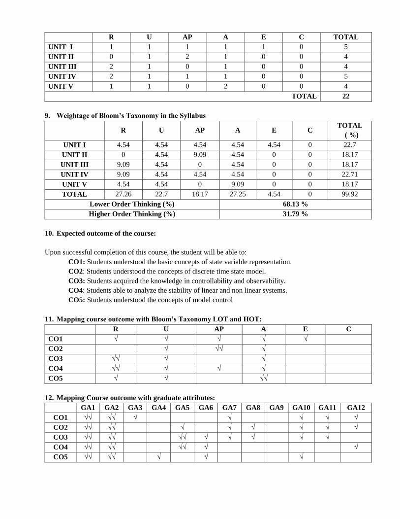
R U AP A E C TOTAL
UNIT I 1 1 1 1 1 0 5
UNIT II 0 1 2 1 0 0 4
UNIT III 2 1 0 1 0 0 4
UNIT IV 2 1 1 1 0 0 5
UNIT V 1 1 0 2 0 0 4
TOTAL 22
9. Weightage of Bloom’s Taxonomy in the Syllabus
R U AP A E C TOTAL
( %)
UNIT I 4.54 4.54 4.54 4.54 4.54 0 22.7
UNIT II 0 4.54 9.09 4.54 0 0 18.17
UNIT III 9.09 4.54 0 4.54 0 0 18.17
UNIT IV 9.09 4.54 4.54 4.54 0 0 22.71
UNIT V 4.54 4.54 0 9.09 0 0 18.17
TOTAL 27.26 22.7 18.17 27.25 4.54 0 99.92
Lower Order Thinking (%) 68.13 %
Higher Order Thinking (%) 31.79 %
10. Expected outcome of the course:
Upon successful completion of this course, the student will be able to:
CO1: Students understood the basic concepts of state variable representation.
CO2: Students understood the concepts of discrete time state model.
CO3: Students acquired the knowledge in controllability and observability.
CO4: Students able to analyze the stability of linear and non linear systems.
CO5: Students understood the concepts of model control
11. Mapping course outcome with Bloom’s Taxonomy LOT and HOT:
R U AP A E C
CO1 √ √ √ √ √
CO2 √ √√ √
CO3 √√ √ √
CO4 √√ √ √ √
CO5 √ √ √√
12. Mapping Course outcome with graduate attributes:
GA1 GA2 GA3 GA4 GA5 GA6 GA7 GA8 GA9 GA10 GA11 GA12
CO1 √√ √√ √ √ √ √ √
CO2 √√ √√ √ √ √ √ √ √
CO3 √√ √√ √√ √ √ √ √ √
CO4 √√ √√ √√ √ √
CO5 √√ √√ √ √ √
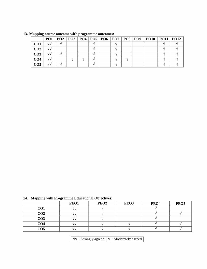
13. Mapping course outcome with programme outcomes:
PO1 PO2 PO3 PO4 PO5 PO6 PO7 PO8 PO9 PO10 PO11 PO12
CO1 √√ √ √ √ √ √
CO2 √√ √ √ √ √
CO3 √√ √ √ √ √ √
CO4 √√ √ √ √ √ √ √ √
CO5 √√ √ √ √ √ √
14. Mapping with Programme Educational Objectives:
PEO1 PEO2 PEO3 PEO4 PEO5
CO1 √√ √ √
CO2 √√ √ √ √
CO3 √√ √ √
CO4 √√ √ √ √ √
CO5 √√ √ √ √ √
√√ Strongly agreed √ Moderately agreed

1. Course pre-requisites : Power Electronics
2. Course learning objectives :
i. To know the DC motor performance with dual converter and chopper.
ii. To understand the Vector controlled induction motor and verify their performance.
iii. Implementation of IGBT based PWM and SVPWM inverter.
iv. To control the speed of BLDC and SRM motor by DSP controller.
3. Expected Level of Output : Practical
4. Department Offered : Electrical and Electronics Engineering
5. Nature of the Course : Group 5 - Practical
Continuous Internal Assessment (CIA): 40 Marks
Semester End Examination (SEE) : 60 Marks
6. List of Experiments:
1. Dual Converter Fed DC Motor Drive
2. Chopper Fed DC Drive
3. DSP controlled AC drive
4. Performance study of Stator Voltage Controlled Induction Motor Drive
5. Vector Controlled Induction Motor Drive
6. IGBT Based Three Phase PWM Inverter
7. IGBT Based Three Phase SVPWM Inverter
8. DSP based speed control of BLDC motor
9. DSP based speed control of SRM motor
10. IGBT based single phase inverters
11. Speed control of DC motor using three phase fully controlled converter
12. Single phase cycloconverters
7. Expected outcome of the course:
Students can able to
CO1: Know the performance of dual converter fed DC motor
CO2: Control the speed of induction motor by Vector control method
CO3: Implement IGBT based inverter
CO4: Vary the speed of BLDC and SRM motor by DSP controller
CO5: Know the operation of cycloconverters
Course Code Course Name Contact Hours
L T P C
17PE211 POWER ELECTRONICS & DRIVES LABORATORY 0 0 3 2


1. Course pre-requisites : Power Electronics
2. Course learning objectives :
i. To understand the characteristics of power diodes and power handling capability of switching
devices
ii. To understand the static and dynamic characteristics of current controlled power semiconductor
devices
iii. To understand the static and dynamic characteristics of voltage controlled power semiconductor
devices
iv. To enable the students for the selection of firing and protection circuit for different power
semiconductor switches
v. To understand the methods of thermal protection for different semiconductor devices.
3. Expected Level of Output : Conceptual Level
4. Department Offered : Electrical &Electronics Engineering
5. Nature of the Course : Group 1 – 100 % Descriptive
Continuous Internal Assessment (CIA) : 40 Marks
Semester End Examination (SEE) : 60 Marks
6. Course Input :
Un
it N
o
Nam
e O
f T
he
Top
ic
Tex
t /
Ref
Book
s
Ch
ap
ter
No
Inst
ruct
ion
al
Hou
rs
Lev
el o
f B
loom
’s
Taxon
om
y
Course
Assessment
Factors
F1
F2
F3
F4
I
INTRODUCTION
Power switching devices overview –
Attributes of an ideal switch, application
requirements
E 1 3 U
9
5 4 4
Power handling capability – (SOA) Device
selection strategy E 1 2 U 5 5 4
On-state and switching losses – EMI due to
switching C 20 1 R 4 2 2
Power diodes - Types, forward and reverse
characteristics, switching characteristics –
rating.
C 20 3 U,AP 5 2 2
CURRENT CONTROLLED DEVICES
Course Code Course Name Contact Hours
L T P C
17PE001 ADVANCED POWER SEMICONDUCTOR DEVICES
3 0 0 3
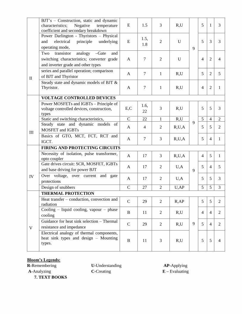
II
BJT’s – Construction, static and dynamic
characteristics; Negative temperature
coefficient and secondary breakdown
E 1.5 3 R,U
9
5 1 3
Power Darlington - Thyristors – Physical
and electrical principle underlying
operating mode,
E 1.5,
1.8 2 U 5 3 3
Two transistor analogy –Gate and
switching characteristics; converter grade
and inverter grade and other types
A 7 2 U 4 2 4
series and parallel operation; comparison
of BJT and Thyristor A 7 1 R,U 5 2 5
Steady state and dynamic models of BJT &
Thyristor.
A 7 1 R,U 4 2 1
III
VOLTAGE CONTROLLED DEVICES
Power MOSFETs and IGBTs – Principle of
voltage controlled devices, construction,
types
E,C 1.6,
22 3 R,U
9
5 5 3
Static and switching characteristics, C 22 1 R,U 5 4 2
Steady state and dynamic models of
MOSFET and IGBTs A 4 2 R,U,A 5 5 2
Basics of GTO, MCT, FCT, RCT and
IGCT. A 7 3 R,U,A 5 4 1
IV
FIRING AND PROTECTING CIRCUITS
Necessity of isolation, pulse transformer,
opto coupler A 17 3 R,U,A
9
4 5 1
Gate drives circuit: SCR, MOSFET, IGBTs
and base driving for power BJT A 17 2 U,A 5 4 5
Over voltage, over current and gate
protections A 17 2 U,A 5 5 3
Design of snubbers C 27 2 U,AP 5 5 3
V
THERMAL PROTECTION
Heat transfer – conduction, convection and
radiation C 29 2 R,AP
9
5 5 2
Cooling – liquid cooling, vapour – phase
cooling B 11 2 R,U 4 4 2
Guidance for heat sink selection – Thermal
resistance and impedance C 29 2 R,U 5 4 2
Electrical analogy of thermal components,
heat sink types and design – Mounting
types.
B 11 3 R,U 5 5 4
Bloom’s Legends:
R-Remembering U-Understanding AP-Applying
A-Analyzing C-Creating E – Evaluating
7. TEXT BOOKS

A. Rashid M.H., "Power Electronics Circuits, Devices and Applications", Prentice Hall India, Third
Edition, New Delhi, 2013.
B. MD Singh and K.B Khanchandani, “Power Electronics”, Tata McGraw Hill, 2001.
REFERENCE BOOKS
C. Ned Mohan, Undeland and Robbin, “Power Electronics: converters, Application and design”, John
Wiley and sons.Inc, Newyork, Reprint 2009
D. B.W. Williams, Power Electronics: Devices, Drivers, Applications and Passive Components, New
York, McGraw-Hill, 1992.
E. Joseph Vithayathil, Power Electronics: Principles and Applications, Delhi, Tata McGraw-Hill,
2010.
WEB RESOURCES
http://www.nptel.ac.in/courses/Webcourse-contents/IITKharagpur/Power Electronics/PDF/
8. Assessing Level of Bloom’s Taxonomy in Numbers:
R U AP A E C TOTAL
UNIT I 1 3 1 0 0 0 5
UNIT II 3 5 0 0 0 0 8
UNIT III 4 4 0 2 0 0 10
UNIT IV 1 4 1 3 0 0 9
UNIT V 4 3 1 0 0 0 8
TOTAL 40
9. Weightage of Bloom’s Taxonomy in the Syllabus
R U AP A E C TOTAL
( %)
UNIT I 2.5 7.5 2.5 0 0 0 12.5
UNIT II 7.5 12.5 0 0 0 0 20
UNIT III 10 10 0 5 0 0 25
UNIT IV 2.5 10 2.5 7.5 0 0 22.5
UNIT V 10 7.5 2.5 0 0 0 20
TOTAL 32.5 47.5 7.5 12.5 0 0 100
Lower Order Thinking (%) 87.5%
Higher Order Thinking (%) 12.5%
10. Expected outcome of the course:
Upon successful completion of this course, the student will be able to:
CO1: Understand the characteristics of power diodes and power handling capability of switching devices
CO2: Understand the static and dynamic characteristics of current controlled power semiconductor devices
CO3: Understand the static and dynamic characteristics of voltage controlled power semiconductor devices
CO4: Enable the students for the selection of firing and protection circuit for different power
semiconductor switches
CO5: Understand the methods of thermal protection for different semiconductor devices
11. Mapping course outcome with Bloom’s Taxonomy LOT and HOT:
R U AP A E C
CO1 √ √ √
CO2 √ √ √
CO3 √ √ √ √
CO4 √ √ √ √ √ √

CO5 √ √ √ √
12. Mapping Course outcome with graduate attributes:
GA1 GA2 GA3 GA4 GA5 GA6 GA7 GA8 GA9 GA10 GA11 GA12
CO1 √√ √ √ √ √ √
CO2 √√ √√ √ √ √ √ √ √
CO3 √√ √√ √ √ √ √ √ √
CO4 √√ √ √√ √√ √ √ √
CO5 √√ √ √ √ √ √ √ √ √
13. Mapping course outcome with programme outcomes:
PO1 PO2 PO3 PO4 PO5 PO6 PO7 PO8 PO9 PO10 PO11 PO12
CO1 √√ √√ √ √ √ √ √ √ √
CO2 √√ √√ √ √ √ √ √ √ √
CO3 √√ √√ √ √ √ √ √ √ √ √ √
CO4 √√ √√ √ √ √ √ √ √ √ √
CO5 √√ √√ √ √ √ √ √ √
14. Mapping with Programme Educational Objectives:
PEO1 PEO2 PEO3 PEO4 PEO5
CO1 √√ √ √
CO2 √√ √ √
CO3 √√ √ √ √
CO4 √√ √ √ √
CO5 √√ √ √ √
√√ Strongly agreed √ Moderately agreed

1. Course pre-requisites : Power Electronics, Control Systems
2. Course learning objectives :
i. To know the tool boxes and programming of files in MATLAB
ii. To design different power converters namely AC to DC, DC to DC and AC to AC converters.
iii. To know about Walsh Domain Operational Method of System
iv. To equip with required skills to derive the criteria for the design of Single-Input Single-Output
Systems from basic fundamentals.
v. To design different power converters namely AC to DC converter using Walsh function
3. Expected Level of Output : Analysis Level
4. Department Offered : Electrical and Electronics Engineering
5. Nature of the Course : Group 3 –20% Descriptive & 40%Analytical & Group 4 –
40%Programming
Continuous Internal Assessment (CIA) : 40 Marks
Semester End Examination (SEE) : 60 Marks
6. Course Input :
Un
it N
o
Nam
e O
f T
he
Top
ic
Tex
t /
Ref
Book
s
Ch
ap
ter
No
Inst
ruct
ion
al
Hou
rs
Lev
el o
f B
loom
’s
Taxon
om
y
Course
Assessment
Factors F
1
F2
F3
F4
I
MATLAB AND SIMULINK
Toolboxes of MATLAB A 1-7 2 R
9
4 3 4
Programming and File processing in
MATLAB A,D 2 U 4 3 4
Model Definition and model analysis using
SIMULINK A,D 2 U,A 4 3 4
S Functions – Converting S-Functions to
block A,D 3 U,Ap 4 3 4
Simulation using MATLAB
Diode Rectifiers – Controlled Rectifiers – A 2,3 3 A, Ap` 9
4 3 4
AC Voltage Controllers– Dc choppers A 4 2 A, Ap 4 3 4
Course Code Course Name Contact Hours
L T P C
17PE002 Simulation of Power Electronic circuits with MATLAB in
Power System
3 0 0 3

II PWM inverters – Voltage and Current
Source Inverts
A 7 2 A, Ap
4 3 4
Zero Current Switching and Zero Voltage
Switching Inverts
A 7 2 A, Ap
4 3 4
III
WALSH DOMAIN OPERATIONAL METHOD OF SYSTEM ANALYSIS
Introduction to Walsh Function -
Rademacher and Walsh Functions -
Applications of Walsh Functions
B 1 3 U,A
9
4 3 4
Time Scaling of Operational Matrices -
Philosophy of the Proposed Walsh Domain
Operational Technique
B 2 2 U,A 4 3 4
Analysis of a First-Order System with
Step Input B 2 2 A 4 3 4
Oscillatory Phenomenon in Walsh Domain
System Analysis B 2 2 A 4 3 4
IV
ANALYSIS OF PULSE-FED SINGLE-INPUT SINGLE-OUTPUT SYSTEMS
Analysis of a First-Order System B 3 3 A
9
4 3 4
Analysis of a Second-Order System B 3 3 A 4 3 4
Pulse-Width Modulated Chopper System B 3 3 A 4 3 4
V
ANALYSIS OF CONTROLLED RECTIFIER CIRCUITS
Representation of a Sine Wave by Walsh
Functions B 4 2 A,Ap
9
4 3 4
Conventional Analysis of Half-Wave
Controlled Rectifier B 4 2 A,Ap 4 3 4
Walsh Domain Analysis of Half-Wave
Controlled Rectifier B 4 2 A,Ap 4 3 4
Walsh Domain Analysis of Full-Wave
Controlled Rectifier B 4 3 A,Ap 4 3 4
Bloom’s Legends:
R-Remembering U-Understanding AP-Applying
A-Analyzing C-Creating E – Evaluating
7. TEXT BOOKS
A. Randall Shaffer, “Fundamentals Of Power Electronics With Matlab Hardcover “ Firewall
Media, 2010
B. D.Anish Deb, Suchismita Ghosh, ”Power Electronic Systems: Walsh Analysis with MATLAB”
CRC Press 2014
REFERENCE BOOKS

C. Adrian B. Biran , “What Every Engineer Should Know about MATLAB® and Simulink” First
Edition , CRC Press, 2010
D. Alok Jain, “Power Electronics: Devices, Circuits And MATLAB Simulations” First Edition
CRC Press, 2010
E. P.S.Bimbra, “Power Electronics”, Khanna Publishers, Fourth Edition, 2012.
WEB RESOURCES
8. Assessing Level of Bloom’s Taxonomy in Numbers:
R U AP A E C TOTAL
UNIT I 1 3 1 1 0 0 6
UNIT II 0 0 4 4 0 0 8
UNIT III 0 2 0 4 0 0 6
UNIT IV 0 0 0 3 0 0 3
UNIT V 0 0 4 4 0 0 8
TOTAL 31
9. Weightage of Bloom’s Taxonomy in the Syllabus
R U AP A E C TOTAL
( %)
UNIT I 3.22 9.6 3.22 3.22 0 0 19.26
UNIT II 0 0 12.9 12.9 0 0 25.8
UNIT III 0 6.45 0 12.9 0 0 19.35
UNIT IV 0 0 0 9.6 0 0 9.6
UNIT V 0 0 12.9 12.9 0 0 25.8
TOTAL 3.22 16.05 29.02 51.52 0 0 99.81
Lower Order Thinking (%) 48.29%
Higher Order Thinking (%) 51.52%
10. Expected outcome of the course:
Upon successful completion of this course, the student will be able to:
CO1: Know Tool boxes and Programming in MATLAB
CO2: Analysis the RMS average values of output voltage and current of the single and three phase rectifiers
and they can also be able to calculate performance parameters and verify the results with MATLAB
CO3: Know Walsh Function
CO4: Analyze the pulse fed single input single output system
CO5: Analysis of Controlled Rectifier Circuits using Walsh function
11. Mapping course outcome with Bloom’s Taxonomy LOT and HOT:
R U AP A E C
CO1 √ √
CO2 √
CO3 √ √
CO4 √ √
CO5 √ √
12. Mapping Course outcome with graduate attributes:
GA1 GA2 GA3 GA4 GA5 GA6 GA7 GA8 GA9 GA10 GA11 GA12

CO1 √ √ √ √ √ √ √
CO2 √ √ √ √ √ √ √ √ √
CO3 √ √ √ √ √ √ √ √ √
CO4 √ √ √ √ √ √ √
CO5 √ √ √ √ √ √ √ √ √
13. Mapping course outcome with programme outcomes:
PO1 PO2 PO3 PO4 PO5 PO6 PO7 PO8 PO9 PO10 PO11 PO12
CO1 √ √ √ √ √ √ √ √ √
CO2 √ √ √ √ √ √ √ √ √
CO3 √ √ √ √ √ √ √ √ √
CO4 √ √ √ √ √ √ √ √ √
CO5 √ √ √ √ √ √ √ √ √
14. Mapping with Programme Educational Objectives:
PEO1 PEO2 PEO3 PEO4 PEO5
CO1 √ √ √ √ √
CO2 √ √ √ √ √
CO3 √ √ √ √ √
CO4 √ √ √ √ √
CO5 √ √ √ √ √
√√ Strongly agreed √ Moderately agreed

1. Course pre-requisites : Power Electronics, Power Systems
2. Course learning objectives :
i. To impart knowledge on different types of converter configurations.
ii. To study the different Applications of converters in HVDC systems
iii. To design and analyze the different types of protection schemes for converters.
iv. To design and chose the best circuit for power system.
v. To impart knowledge on compensation by a series capacitor.
3. Expected Level of Output : Conceptual Level
4. Department Offered : Electrical and Electronics Engineering
5. Nature of the Course : Group 1 – 100 % Descriptive
Continuous Internal Assessment (CIA) : 40 Marks
Semester End Examination (SEE) : 60 Marks
6. Course Input :
Un
it N
o
Nam
e O
f T
he
Top
ic
Tex
t /
Ref
Book
s
Ch
ap
ter
No
Inst
ruct
ion
al
Hou
rs
Lev
el o
f B
loom
’s
Taxon
om
y
Course
Assessment
Factors
F1
F2
F3
F4
I
INTRODUCTION
High Power drives for Power systems
controllers B 1,2 3 R
7
3 1 2
Characteristics B 2 2 U 3 2 3
Configuration for Large power control A 4 2 A 2 1 1
II
SINGLE PHASE AND THREE PHASE CONVERTERS
Properties – Current and voltage harmonics
Effect of source and load impendence A 8 3 R , U
10
3 2 3
Choice of best circuit for power systems-
Converter Control - Gate Control A 3,4 2 A,AP 4 3 2
Basic means of Control – Control
characteristics – Stability of control –
Reactive power control - Applications of
A 4 3 A,E 3 3 2
Course Code Course Name Contact Hours
L T P C
17PE003 APPLICATIONS OF POWER ELECTRONICS IN POWER
SYSTEMS
3
0
0
3
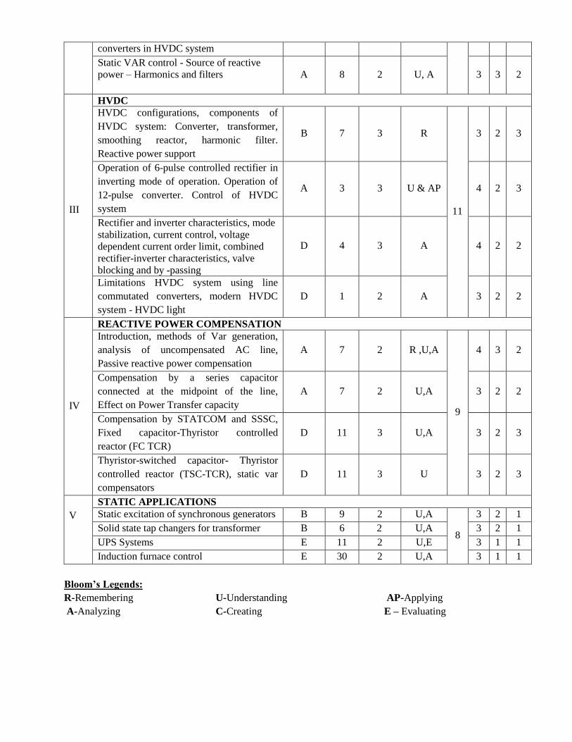
converters in HVDC system
Static VAR control - Source of reactive
power – Harmonics and filters
A 8 2 U, A 3 3 2
III
HVDC
HVDC configurations, components of
HVDC system: Converter, transformer,
smoothing reactor, harmonic filter.
Reactive power support
B 7 3 R
11
3 2 3
Operation of 6-pulse controlled rectifier in
inverting mode of operation. Operation of
12-pulse converter. Control of HVDC
system
A 3 3 U & AP 4 2 3
Rectifier and inverter characteristics, mode
stabilization, current control, voltage
dependent current order limit, combined
rectifier-inverter characteristics, valve
blocking and by -passing
D 4 3 A 4 2 2
Limitations HVDC system using line
commutated converters, modern HVDC
system - HVDC light
D 1 2 A 3 2 2
IV
REACTIVE POWER COMPENSATION
Introduction, methods of Var generation,
analysis of uncompensated AC line,
Passive reactive power compensation
A 7 2 R ,U,A
9
4 3 2
Compensation by a series capacitor
connected at the midpoint of the line,
Effect on Power Transfer capacity
A 7 2 U,A 3 2 2
Compensation by STATCOM and SSSC,
Fixed capacitor-Thyristor controlled
reactor (FC TCR)
D 11 3 U,A 3 2 3
Thyristor-switched capacitor- Thyristor
controlled reactor (TSC-TCR), static var
compensators
D 11 3 U 3 2 3
V
STATIC APPLICATIONS
Static excitation of synchronous generators B 9 2 U,A
8
3 2 1
Solid state tap changers for transformer B 6 2 U,A 3 2 1
UPS Systems E 11 2 U,E 3 1 1
Induction furnace control E 30 2 U,A 3 1 1
Bloom’s Legends:
R-Remembering U-Understanding AP-Applying
A-Analyzing C-Creating E – Evaluating
7. TEXT BOOKS
A. K.R. Padiyar, HVDC Power Transmission System – Technology and System Interaction, New
Delhi, New Age International, 2002.
B. Ned Mohan, Electric power system, New York, John Wiley and Sons, 2012.
REFERENCE BOOKS
C. S. Kamakshaiah, V. Kamaraj , HVDC Transmission, New Delhi, Tata Mc Graw-Hill Education
Pvt Ltd, 2011
D. B. Ned Mohan, Power electronic converters Applications and Design, New York, John Wiley
and Sons, 2013.
E. Mohd. Hasan Ali, Bin Wu, Roger A. Dougal, An Overview of SMES Applications in Power
and Energy Systems, IEEE Transactions on Sustainable Energy, vol. 1, no. 1, April 2010.
WEB RESOURCES
nptel.ac.in/ High Voltage DC Transmission/ Industrial drives
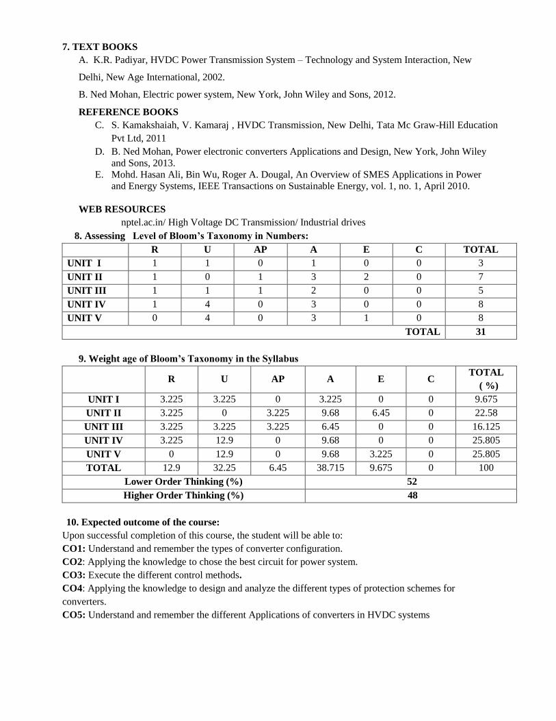
8. Assessing Level of Bloom’s Taxonomy in Numbers:
R U AP A E C TOTAL
UNIT I 1 1 0 1 0 0 3
UNIT II 1 0 1 3 2 0 7
UNIT III 1 1 1 2 0 0 5
UNIT IV 1 4 0 3 0 0 8
UNIT V 0 4 0 3 1 0 8
TOTAL 31
9. Weight age of Bloom’s Taxonomy in the Syllabus
R U AP A E C TOTAL
( %)
UNIT I 3.225 3.225 0 3.225 0 0 9.675
UNIT II 3.225 0 3.225 9.68 6.45 0 22.58
UNIT III 3.225 3.225 3.225 6.45 0 0 16.125
UNIT IV 3.225 12.9 0 9.68 0 0 25.805
UNIT V 0 12.9 0 9.68 3.225 0 25.805
TOTAL 12.9 32.25 6.45 38.715 9.675 0 100
Lower Order Thinking (%) 52
Higher Order Thinking (%) 48
10. Expected outcome of the course:
Upon successful completion of this course, the student will be able to:
CO1: Understand and remember the types of converter configuration.
CO2: Applying the knowledge to chose the best circuit for power system.
CO3: Execute the different control methods.
CO4: Applying the knowledge to design and analyze the different types of protection schemes for
converters.
CO5: Understand and remember the different Applications of converters in HVDC systems
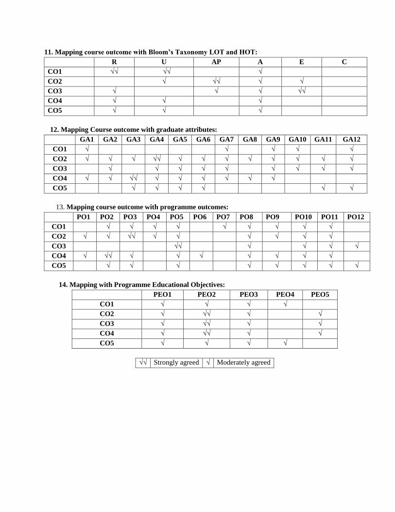
11. Mapping course outcome with Bloom’s Taxonomy LOT and HOT:
R U AP A E C
CO1 √√ √√ √
CO2 √ √√ √ √
CO3 √ √ √ √√
CO4 √ √ √
CO5 √ √ √
12. Mapping Course outcome with graduate attributes:
GA1 GA2 GA3 GA4 GA5 GA6 GA7 GA8 GA9 GA10 GA11 GA12
CO1 √ √ √ √ √
CO2 √ √ √ √√ √ √ √ √ √ √ √ √
CO3 √ √ √ √ √ √ √ √ √
CO4 √ √ √√ √ √ √ √ √ √
CO5 √ √ √ √ √ √
13. Mapping course outcome with programme outcomes:
PO1 PO2 PO3 PO4 PO5 PO6 PO7 PO8 PO9 PO10 PO11 PO12
CO1 √ √ √ √ √ √ √ √ √
CO2 √ √ √√ √ √ √ √ √ √
CO3 √√ √ √ √ √
CO4 √ √√ √ √ √ √ √ √ √
CO5 √ √ √ √ √ √ √ √
14. Mapping with Programme Educational Objectives:
PEO1 PEO2 PEO3 PEO4 PEO5
CO1 √ √ √ √
CO2 √ √√ √ √
CO3 √ √√ √ √
CO4 √ √√ √ √
CO5 √ √ √ √
√√ Strongly agreed √ Moderately agreed

1. Course pre-requisites : Power System Generation, Transmission, Distribution &
Analysis
2. Course learning objectives :
i. To understand the concepts of FACTS
ii. To expose the students to the applications of FACTS controllers in power systems
iii. To learn about shunt & series compensation schemes
iv. To make the students’ learn the simulation of FACTS Controllers
v. To understand the phenomenon of SSR & its mitigation
3. Expected Level of Output : Conceptual Level
4. Department Offered : Electrical & Electronics Engineering
5. Nature of the Course : Group 1 – 100 % Descriptive
Continuous Internal Assessment (CIA) : 40 Marks
Semester End Examination (SEE) : 60 Marks
6. Course Input :
Un
it N
o
Nam
e O
f T
he
Top
ic
Tex
t /
Ref
Book
s
Ch
ap
ter
No
Inst
ruct
ion
al
Hou
rs
Lev
el o
f B
loom
’s
Taxon
om
y
Course
Assessment
Factors
F1
F2
F3
F4
I
INTRODUCTION
Introduction A 1 2 U
9
5 4 3
Electrical Transmission Network–
Necessity A 1 1 U 5 5 3
Power Flow in AC system & Relative
importance of controllable parameter A 1 2 U 4 4 2
Opportunities for FACTS, Possible
benefits for FACTS Technology & Types
of FACTS Controllers
A 1 4 U 5 5 3
II
STATIC VAR COMPENSATION
Need for compensation – introduction to
shunt & series compensation A 2 2 U
9
5 5 3
Objectives of shunt & series compensation A 2 2 R,U 4 3 2
Configuration & Operating characteristics
– Thyristor Controlled
Reactor (TCR),Thyristor Switched
Capacitor (TSC)
A 2,3 3 A 5 4 2
Course Code Course Name Contact Hours
L T P C
17PE004 FLEXIBLE AC TRANSMISSION SYSTEMS 3 0 0 3
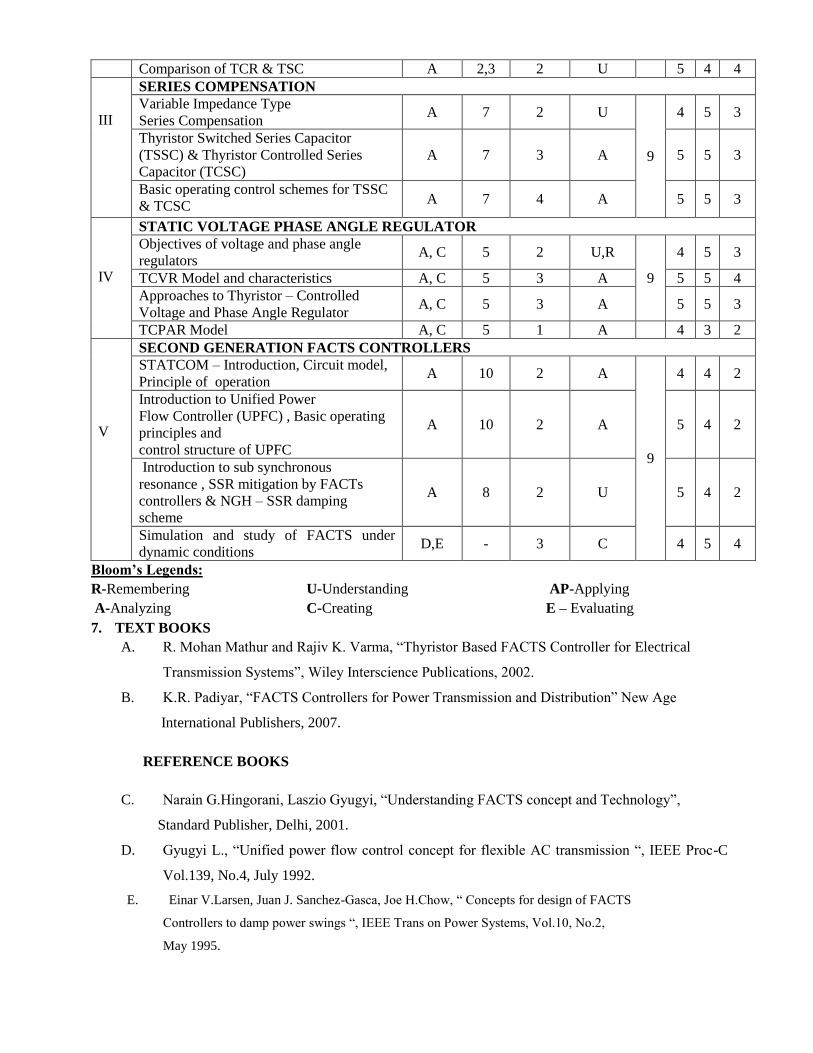
Comparison of TCR & TSC A 2,3 2 U 5 4 4
III
SERIES COMPENSATION
Variable Impedance Type
Series Compensation A 7 2 U
9
4 5 3
Thyristor Switched Series Capacitor
(TSSC) & Thyristor Controlled Series
Capacitor (TCSC)
A 7 3 A 5 5 3
Basic operating control schemes for TSSC
& TCSC A 7 4 A 5 5 3
IV
STATIC VOLTAGE PHASE ANGLE REGULATOR
Objectives of voltage and phase angle
regulators A, C 5 2 U,R
9
4 5 3
TCVR Model and characteristics A, C 5 3 A 5 5 4
Approaches to Thyristor – Controlled
Voltage and Phase Angle Regulator A, C 5 3 A 5 5 3
TCPAR Model A, C 5 1 A 4 3 2
V
SECOND GENERATION FACTS CONTROLLERS
STATCOM – Introduction, Circuit model,
Principle of operation A 10 2 A
9
4 4 2
Introduction to Unified Power
Flow Controller (UPFC) , Basic operating
principles and
control structure of UPFC
A 10 2 A 5 4 2
Introduction to sub synchronous
resonance , SSR mitigation by FACTs
controllers & NGH – SSR damping
scheme
A 8 2 U 5 4 2
Simulation and study of FACTS under
dynamic conditions D,E - 3 C 4 5 4
Bloom’s Legends:
R-Remembering U-Understanding AP-Applying
A-Analyzing C-Creating E – Evaluating
7. TEXT BOOKS
A. R. Mohan Mathur and Rajiv K. Varma, “Thyristor Based FACTS Controller for Electrical
Transmission Systems”, Wiley Interscience Publications, 2002.
B. K.R. Padiyar, “FACTS Controllers for Power Transmission and Distribution” New Age
International Publishers, 2007.
REFERENCE BOOKS
C. Narain G.Hingorani, Laszio Gyugyi, “Understanding FACTS concept and Technology”,
Standard Publisher, Delhi, 2001.
D. Gyugyi L., “Unified power flow control concept for flexible AC transmission “, IEEE Proc-C
Vol.139, No.4, July 1992.
E. Einar V.Larsen, Juan J. Sanchez-Gasca, Joe H.Chow, “ Concepts for design of FACTS
Controllers to damp power swings “, IEEE Trans on Power Systems, Vol.10, No.2,
May 1995.

8. Assessing Level of Bloom’s Taxonomy in Numbers:
R U AP A E C TOTAL
UNIT I 0 4 0 0 0 0 4
UNIT II 1 3 0 1 0 0 5
UNIT III 0 1 0 2 0 0 3
UNIT IV 1 1 0 3 0 0 5
UNIT V 0 1 0 2 0 1 4
TOTAL 21
9. Weight age of Bloom’s Taxonomy in the Syllabus
R U AP A E C TOTAL
( %)
UNIT I 0 19.05 0 0 0 0 19.05
UNIT II 4.76 14.29 0 4.76 0 0 23.81
UNIT III 0 4.76 0 9.52 0 0 14.28
UNIT IV 4.76 4.76 0 14.29 0 0 23.81
UNIT V 0 4.76 0 9.52 0 4.76 19.04
TOTAL 9.52 47.62 0 38.09 0 4.76 100
Lower Order Thinking (%) 100 %
Higher Order Thinking (%) NIL
10. Expected outcome of the course:
Upon successful completion of this course, the student will be able to:
CO1: Understand and analyze the concept of FACTS.
CO2: To understand the various types of compensation schemes.
CO3: Implement various FACTS controllers.
CO4: Applying the knowledge gained to simulate various FACTS controllers.
CO5: Understand about the phenomena of sub synchronous resonance
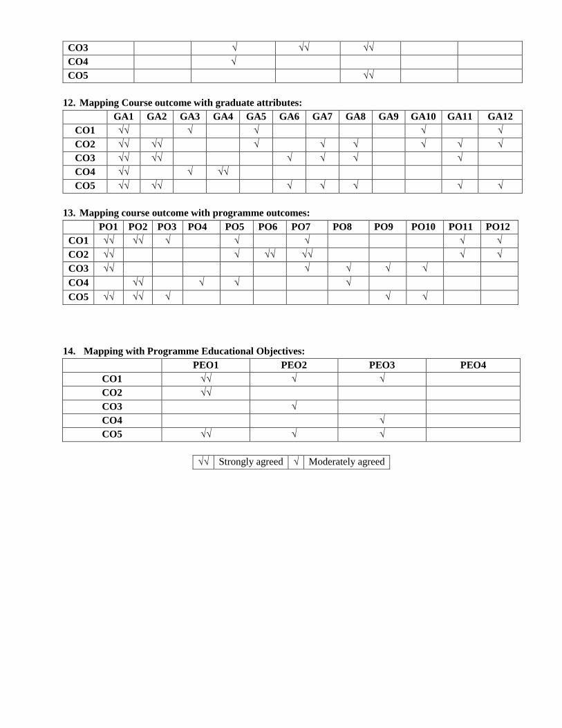
11. Mapping course outcome with Bloom’s Taxonomy LOT and HOT:
R U AP A E C
CO1 √√ √
CO2 √
CO3 √√ √ √
CO4 √√ √
CO5 √√
12. Mapping Course outcome with graduate attributes:
GA1 GA2 GA3 GA4 GA5 GA6 GA7 GA8 GA9 GA10 GA11 GA12
CO1 √
CO2 √
CO3 √ √ √ √
CO4 √ √ √ √√
CO5 √
13. Mapping course outcome with programme outcomes:

PO1 PO2 PO3 PO4 PO5 PO6 PO7 PO8 PO9 PO10 PO11 PO12
CO1 √ √√ √
CO2 √
CO3 √ √√ √ √√ √
CO4 √ √√ √√ √ √√
CO5 √ √√ √
14. Mapping with Programme Educational Objectives:
PEO1 PEO2 PEO3 PEO4 PEO5
CO1 √ √√ √√
CO2 √ √√ √
CO3 √ √√
CO4 √ √ √√ √
CO5 √ √√ √√
√√ Strongly agreed √ Moderately agreed

1. Course pre-requisites :Analysis of Power Converters, Analysis of Inverters
2. Course learning objectives :
i. To understand the concept of DC transmission systems.
ii. To analyze the control strategies in a DC transmission.
iii. To model and analyze the power flow concept in DC transmission systems.
iv. Apply the knowledge to overcome the DC transmission problems.
v. To Analyze the DC transmission system and their problems by simulation techniques
3. Expected Level of Output :Conceptual Level
4. Department Offered :EEE
5. Nature of the Course :A. Group 1 – 100 % Descriptive
Continuous Internal Assessment (CIA) : 40 Marks
Semester End Examination (SEE) : 60 Marks
6. Course Input :
Un
it N
o
Nam
e O
f T
he
Top
ic
Tex
t /
Ref
Book
s
Ch
ap
ter
No
Inst
ruct
ion
al
Hou
rs
Lev
el o
f B
loom
’s
Taxon
om
y
Course
Assessment
Factors
F1
F2
F3
F4
I
DC POWER TRANSMISSION TECHNOLOGY
Introduction - Comparison of AC and DC
transmission – Application of DC
transmission
A
1
1
R, U
6
5 4 4
Description of DC transmission system –
A 1 1 U 4 3 3
Planning for HVDC transmission A 1 1 E 4 3 1
Modern trends in DC transmission – DC
breakers A 1 1 A 4 3 1
Operating problems A 1 1 A 4 2 0
HVDC transmission based on voltage
source converters. A 1 1 E 4 1 3
ANALYSIS OF HVDC CONVERTERS AND HVDC SYSTEM CONTROL
Pulse number, choice of converter
configuration A 2 2 U
12
4 3 2
Simplified analysis of Graetz circuit A 2 1 A 3 1 0
Course Code Course Name Contact Hours
L T P C
17PE005 HIGH VOLTAGE DIRECT CURRENT TRANSMISSION 3 0 0 3

II
Converter bridge characteristics –
characteristics of a twelve pulse converter. A 3 2 A 3 1 1
Detailed Analysis of converters A 3 1 A 4 2 2
General principles of DC link control A 4 1 U 4 3 1
Converter control characteristics A 4 1 A 4 3 2
System
control hierarchy - Firing angle control –
A 4 1 U,A 5 3 3
Current and extinction angle control –
A 4 1 U,A 4 3 2
Generation of harmonics and filtering - A 4 1 U,E 4 2 2
power control – Higher level controllers A 4 1 U,A 4 2 1
III
MULTITERMINAL DC SYSTEMS
Introduction A 9 1 R
9
5 3 0
Potential applications of MTDC systems A 9 2 A 4 3 2
Types of MTDC systems
A 9 2 U, Ap 5 3 1
Control and protection of MTDC systems A 9 2 A, Ap 5 2 1
Study of MTDC systems A 9 2 A 5 3 0
IV
POWER FLOW ANALYSIS IN AC/DC SYSTEMS
Per unit system for DC Quantities A 10 1 U
9
5 4 3
Modeling of DC links A 10 2 A 5 4 4
Solution of DC load flow A 10 2 A 5 3 1
Solution of AC-DC power flow A 10 2 A 5 3 1
Case studies A 10
2
AP 5 3 0
V
SIMULATION OF HVDC SYSTEMS
Introduction A 11 1 U
9
5 5 0
System simulation: Philosophy and tools A 11 2 A, AP 4 3 1
HVDC system simulation A 11 2 A, C 5 3 2
Modeling of HVDC systems for digital
dynamic simulation A 11 2 A, E 4 3 2
Dynamic in traction
between DC and AC systems. A 11 2 A, E 4 2 0

Bloom’s Legends:
R-Remembering U-Understanding AP-Applying
A-Analyzing C-Creating E – Evaluating
7. TEXT BOOKS
A. K.R.Padiyar , “HVDC Power Transmission Systems”, New Age International (P) Ltd., New
Delhi, 2012.
B. Kamakshaiah S, Kamaraju V,”HVDC transmission”, Tata McGraw Hill edu.pvt.ltd, 2011.
REFERENCE BOOKS
C. P. Kundur, “Power System Stability and Control”, McGraw-Hill, 1993.
D. Erich Uhlmann, “Power Transmission by Direct Current”, BS Publications, 2004.
E. V.K.Sood, HVDC and FACTS controllers – Applications of Static Converters in
Power System, APRIL 2004, Kluwer Academic Publishers.
8. Assessing Level of Bloom’s Taxonomy in Numbers:
R U AP A E C TOTAL
UNIT I 1 2 0 2 2 0 7
UNIT II 0 6 0 7 1 0 14
UNIT III 1 1 2 3 0 0 7
UNIT IV 0 1 1 3 0 0 5
UNIT V 0 1 1 4 2 1 9
TOTAL 42
9. Weightage of Bloom’s Taxonomy in the Syllabus
R U AP A E C TOTAL
( %)
UNIT I 2.38 4.76 0 4.76 4.76 0 16.66
UNIT II 0 14.29 0 16.67 2.38 0 33.34
UNIT III 2.38 2.38 4.76 7.14 0 0 16.66
UNIT IV 0 2.38 2.38 7.14 0 0 11.9
UNIT V 0 2.38 2.38 9.52 4.76 2.38 21.42
TOTAL 4.76 26.19 9.52 45.23 11.9 2.38 100
Lower Order Thinking (%) 40.47%
Higher Order Thinking (%) 59.51%
10. Expected outcome of the course:
Upon successful completion of this course, the student will be able to:
CO1: Understand about the DC transmission system.
CO2: Apply knowledge to find the solution of the power flow problems.
CO3: Create and evaluate long distance DC transmission.
CO4: Applying the knowledge gained about the DC transmission to analyze about it.
CO5: To Analyze the DC transmission system and their problems by simulation techniques.
11. Mapping course outcome with Bloom’s Taxonomy LOT and HOT:
R U AP A E C
CO1 √ √
CO2 √ √
CO3 √ √√ √√
CO4 √
CO5 √√
12. Mapping Course outcome with graduate attributes:
GA1 GA2 GA3 GA4 GA5 GA6 GA7 GA8 GA9 GA10 GA11 GA12
CO1 √√ √ √ √ √
CO2 √√ √√ √ √ √ √ √ √
CO3 √√ √√ √ √ √ √
CO4 √√ √ √√
CO5 √√ √√ √ √ √ √ √
13. Mapping course outcome with programme outcomes:
PO1 PO2 PO3 PO4 PO5 PO6 PO7 PO8 PO9 PO10 PO11 PO12
CO1 √√ √√ √ √ √ √ √
CO2 √√ √ √√ √√ √ √
CO3 √√ √ √ √ √
CO4 √√ √ √ √
CO5 √√ √√ √ √ √
14. Mapping with Programme Educational Objectives:
PEO1 PEO2 PEO3 PEO4
CO1 √√ √ √
CO2 √√
CO3 √
CO4 √
CO5 √√ √ √
√√ Strongly agreed √ Moderately agreed
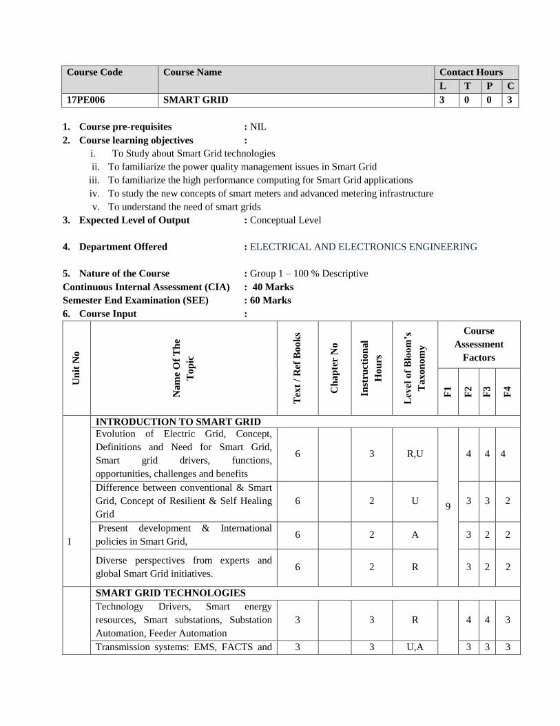
1. Course pre-requisites : NIL
2. Course learning objectives :
i. To Study about Smart Grid technologies
ii. To familiarize the power quality management issues in Smart Grid
iii. To familiarize the high performance computing for Smart Grid applications
iv. To study the new concepts of smart meters and advanced metering infrastructure
v. To understand the need of smart grids
3. Expected Level of Output : Conceptual Level
4. Department Offered : ELECTRICAL AND ELECTRONICS ENGINEERING
5. Nature of the Course : Group 1 – 100 % Descriptive
Continuous Internal Assessment (CIA) : 40 Marks
Semester End Examination (SEE) : 60 Marks
6. Course Input :
Un
it N
o
Nam
e O
f T
he
Top
ic
Tex
t /
Ref
Book
s
Ch
ap
ter
No
Inst
ruct
ion
al
Hou
rs
Lev
el o
f B
loom
’s
Taxon
om
y
Course
Assessment
Factors
F1
F2
F3
F4
I
INTRODUCTION TO SMART GRID
Evolution of Electric Grid, Concept,
Definitions and Need for Smart Grid,
Smart grid drivers, functions,
opportunities, challenges and benefits
6 3 R,U
9
4 4 4
Difference between conventional & Smart
Grid, Concept of Resilient & Self Healing
Grid
6 2 U 3 3 2
Present development & International
policies in Smart Grid, 6 2 A 3 2 2
Diverse perspectives from experts and
global Smart Grid initiatives. 6 2 R 3 2 2
SMART GRID TECHNOLOGIES
Technology Drivers, Smart energy
resources, Smart substations, Substation
Automation, Feeder Automation
3 3 R
4 4 3
Transmission systems: EMS, FACTS and 3 3 U,A 3 3 3
Course Code Course Name Contact Hours
L T P C
17PE006 SMART GRID 3 0 0 3
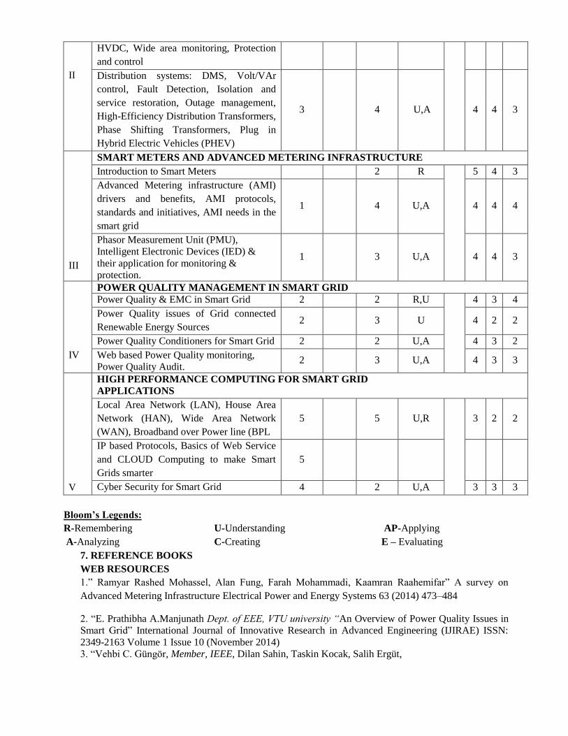
II
HVDC, Wide area monitoring, Protection
and control
Distribution systems: DMS, Volt/VAr
control, Fault Detection, Isolation and
service restoration, Outage management,
High-Efficiency Distribution Transformers,
Phase Shifting Transformers, Plug in
Hybrid Electric Vehicles (PHEV)
3 4 U,A 4 4 3
III
SMART METERS AND ADVANCED METERING INFRASTRUCTURE
Introduction to Smart Meters 2 R
5 4 3
Advanced Metering infrastructure (AMI)
drivers and benefits, AMI protocols,
standards and initiatives, AMI needs in the
smart grid
1 4 U,A 4 4 4
Phasor Measurement Unit (PMU),
Intelligent Electronic Devices (IED) &
their application for monitoring &
protection.
1 3 U,A 4 4 3
IV
POWER QUALITY MANAGEMENT IN SMART GRID
Power Quality & EMC in Smart Grid 2 2 R,U
4 3 4
Power Quality issues of Grid connected
Renewable Energy Sources 2 3 U 4 2 2
Power Quality Conditioners for Smart Grid 2 2 U,A 4 3 2
Web based Power Quality monitoring,
Power Quality Audit. 2 3 U,A 4 3 3
V
HIGH PERFORMANCE COMPUTING FOR SMART GRID
APPLICATIONS
Local Area Network (LAN), House Area
Network (HAN), Wide Area Network
(WAN), Broadband over Power line (BPL
5 5 U,R
3 2 2
IP based Protocols, Basics of Web Service
and CLOUD Computing to make Smart
Grids smarter
5
Cyber Security for Smart Grid 4 2 U,A 3 3 3
Bloom’s Legends:
R-Remembering U-Understanding AP-Applying
A-Analyzing C-Creating E – Evaluating
7. REFERENCE BOOKS
WEB RESOURCES
1.” Ramyar Rashed Mohassel, Alan Fung, Farah Mohammadi, Kaamran Raahemifar” A survey on
Advanced Metering Infrastructure Electrical Power and Energy Systems 63 (2014) 473–484
2. “E. Prathibha A.Manjunath Dept. of EEE, VTU university “An Overview of Power Quality Issues in
Smart Grid” International Journal of Innovative Research in Advanced Engineering (IJIRAE) ISSN:
2349-2163 Volume 1 Issue 10 (November 2014)
3. “Vehbi C. Güngör, Member, IEEE, Dilan Sahin, Taskin Kocak, Salih Ergüt,

Concettina Buccella, Senior Member, IEEE, Carlo Cecati, Fellow, IEEE, and Gerhard P. Hancke, Senior
Member, IEEE” Smart Grid Technologies: Communication Technologies and Standards IEEE
Transactions on Industrial Informatics, Vol. 7, No. 4, November 2011
4.“Ye Yan, Yi Qian, Hamid Sharif and David Tipper” A Survey on Cyber Security for Smart Grid
Communications IEEE Communications Surveys & Tutorials, Vol. 14, No. 4, Fourth Quarter 2012
5.” Murat Kuzlu, Manisa Pipattanasomporn, Saifur Rahman” Communication network requirements for
major smart grid applications in HAN, NAN and WAN journal homepage:
www.elsevier.com/locate/comnet
6. www.wikipedia.org
8. Assessing Level of Bloom’s Taxonomy in Numbers:
R U AP A E C TOTAL
UNIT I 1 2 1 0 0 0 4
UNIT II 1 3 2 0 0 0 6
UNIT III 1 3 1 0 0 0 5
UNIT IV 1 3 1 0 0 0 5
UNIT V 1 2 1 0 0 0 4
TOTAL 24
9. Weightages of Bloom’s Taxonomy in the Syllabus
R U AP A E C TOTAL
( %)
UNIT I 4.16 8.33 4.16 0 0 0 16.65
UNIT II 4.16 12.5 8.33 0 0 0 24.99
UNIT III 4.16 12.5 4.16 0 0 0 20.82
UNIT IV 4.16 12.5 4.16 0 0 0 20.82
UNIT V 4.16 8.33 4.16 0 0 0 16.65
TOTAL 20.8 54.16 24.97 0 0 0 99.93
Lower Order Thinking (%) 99.93
Higher Order Thinking (%) 0.07
10. Expected outcome of the course:
Upon successful completion of this course, the student will be able to:
CO1: Understand about Smart Grid technologies, different smart meters and advanced metering
infrastructure
CO2: Familiarize with the technologies of smart grid
CO3: Understand the concept of smart meters
CO4: Familiarize with power quality management
CO5: Will know the security system for smart grid
11. Mapping course outcome with Bloom’s Taxonomy LOT and HOT:
R U AP A E C
CO1 √√ √
CO2 √ √√
CO3 √√ √
CO4 √√
CO5 √ √√

12. Mapping Course outcome with graduate attributes:
GA1 GA2 GA3 GA4 GA5 GA6 GA7 GA8 GA9 GA10 GA11 GA12
CO1 √√ √ √√ √ √√ √ √ √ √
CO2 √√ √ √√ √ √ √ √ √ √
CO3 √√ √√ √ √ √ √
CO4 √√ √ √√ √√ √
CO5 √√ √ √ √√ √√ √
13. Mapping course outcome with programme outcomes:
PO1 PO2 PO3 PO4 PO5 PO6 PO7 PO8 PO9 PO10 PO11 PO12
CO1 √√ √√ √ √ √√ √ √√ √ √ √ √
CO2 √√ √√ √ √√ √ √ √
CO3 √√ √√ √√ √ √ √ √ √√ √ √ √
CO4 √√ √√ √ √ √ √ √
CO5 √ √√ √√ √√ √ √√ √√ √ √√ √ √
14. Mapping with Programme Educational Objectives:
PEO1 PEO2 PEO3 PEO4 PEO5
CO1 √√ √ √ √ √
CO2 √√ √ √
CO3 √√ √ √ √
CO4 √√ √ √
CO5 √√ √ √√ √ √√
√√ Strongly agreed √ Moderately agreed

1. Course pre-requisites : Power Electronics, Power Generation Systems & AC Machines
2. Course learning objectives :
i. To expose the students to the applications of power electronics in power systems
ii. To understand the concepts of machines for renewable energy sources
iii. To understand & design the PV systems
iv. To understand & design the wind energy systems
v. To understand & implement the concepts of wind and solar power systems
3. Expected Level of Output : Conceptual Level
4. Department Offered : M.E. (Power Electronics and Drives)
5. Nature of the Course : Group 1 – 100 % Descriptive
Continuous Internal Assessment (CIA) : 40 Marks
Semester End Examination (SEE) : 60 Marks
6. Course Input :
Un
it N
o
Nam
e O
f T
he
Top
ic
Tex
t /
Ref
Book
s
Ch
ap
ter
No
Inst
ruct
ion
al
Hou
rs
Lev
el o
f
Blo
om
’s
Taxon
om
y Course
Assessment
Factors
F1
F2
F3
F4
I
INTRODUCTION
Environmental aspects of electric
energy conversion A,C 2,1 1 A
9
1 1 0
Impacts of renewable energy generation
on environment C 1 1 A 1 1 0
Qualitative study of renewable energy
resources: Solar C,D 4,5,6,1 1 U 2 4 5
Qualitative study of renewable energy
resources: Wind C,D 7,2 1 U 2 4 5
Qualitative study of renewable energy
resources: Ocean C,D 10,1 1 U
2 0 2
Qualitative study of renewable energy
resources: Bio Mass C,D 8,3 1 U 2 1 1
Qualitative study of renewable energy
resources: Fuel Cell C 12 1 U 2 1 1
Qualitative study of renewable energy
resources: Hybrid renewable energy
systems
A,C,D 28,7,5 2 U 2 4 4
ELECTRICAL MACHINES FOR RENEWABLE ENERGY CONVERSION
Review of reference theory
fundamentals B 6 2 R 9 5 2 4
Course Code Course Name Contact Hours
L T P C
17PE007 POWER ELECTRONICS FOR RENEWABLE ENERGY
SYSTEMS 3 0 0 3

II Principle of operation and analysis:
Induction Generator B 6 4 A 5 2 5
Principle of operation and analysis:
Synchronous Generator B 6 3 A 4 2 4
III
ANALYSIS OF PV SYSTEMS
Solar: Block diagram of solar photo
voltaic system A 27,28 2 A
9
5 5 4
Principle of operation - Stand alone
system A 27,28 2 A 3 5 4
Principle of operation - Grid connected
system A 27,28 2 A 3 5 4
Selection of inverter - battery and array
sizing A 27,28 2 A 2 2 5
Types of converters in PV system. A 227,8 1 C 2 4 5
IV
ANALYSIS OF WIND SYSTEMS
Stand alone operation of fixed speed
wind energy conversion systems A 28 2 U
9
4 2 0
Stand alone operation of variable speed
wind energy conversion systems A 28 2 U 5 2 0
Grid connection system and its issues A 28 1 R 1 0 0
Grid integrated with PMSG Based
WECS A 28 1 A 4 1 2
Grid integrated with SCIG Based
WECS A 28 1 A 4 1 2
Grid integrated with DFIG Based
WECS A 28 1 A 4 1 2
Types of inverters in wind system A 28 1 C 3 1 5
V
CASE STUDIES IN RENEWABLE ENERGY SOURCES
Case studies of Wind - Maximum
Power Point Tracking (MPPT)
Techniques
A 28 2 AP
9
5 2 5
Case studies of Solar - Maximum
Power Point Tracking (MPPT)
Techniques
A 27,28 3 AP 5 2 5
Case studies of Solar - Inverter
technologies A 27,28 1 A 5 2 5
Case studies of Solar - Converter
technologies A 27,28 1 A 5 2 5
Case studies of Wind - Inverter
technologies A 28 1 A 5 3 5
Case studies of Wind - Converter
technologies A 28,30 1 A 5 3 5
Bloom’s Legends:
R-Remembering U-Understanding AP-Applying
A-Analyzing C-Creating E – Evaluating
7. TEXT BOOKS
A. Muhammad H. Rashid, “Power Electronics Handbook”, Elsevier, 2011.
B. S N Bard, D Kastha, S Banerjee, “Wind Electrical Systems”, Oxford University Press, 2012.
REFERENCE BOOKS
C. B H Khan, “Non-Conventional Energy Resources”, the McGraw Hill Companies – 2nd
edition
2009.

D. G D Rai, “Non-Conventional Energy Sources”, Khanna Publishers, 2011.
E. Ali Keyhani, “Design of Smart Power Grid Renewable Energy Systems”, John Wiley & Sons,
2011.
WEB RESOURCES
8. Assessing Level of Bloom’s Taxonomy in Numbers:
R U AP A E C TOTAL
UNIT I 0 6 0 2 0 0 8
UNIT II 1 0 0 2 0 0 3
UNIT III 0 0 0 4 0 1 5
UNIT IV 1 2 0 3 0 1 7
UNIT V 0 0 2 4 0 0 6
TOTAL 29
9. Weight age of Bloom’s Taxonomy in the Syllabus
R U AP A E C TOTAL
( %)
UNIT I 0 20.69 0 6.89 0 0 27.59
UNIT II 3.44 0 0 6.89 0 0 10.33
UNIT III 0 0 0 13.79 0 3.44 17.23
UNIT IV 3.44 6.89 0 10.34 0 3.44 24.11
UNIT V 0 0 6.89 13.79 0 0 20.68
TOTAL 6.88 27.58 6.89 51.70 0 6.88 100
Lower Order Thinking (%) 41.35%
Higher Order Thinking (%) 58.58%
10. Expected outcome of the course:
Upon successful completion of this course, the student will be able to:
CO1: Understand the concepts of renewable energy systems.
CO2: Understand the concepts of different types of Electrical Machines employed for Renewable Energy
Conversion Systems.
CO3: Understand the concepts of Standalone, Grid connected PV Systems.
CO4: Understand the concepts of Standalone, Grid connected Wind Systems.
CO5: Design a system, component or process to meet desired needs.
11. Mapping course outcome with Bloom’s Taxonomy LOT and HOT:
R U AP A E C
CO1 √ √
CO2 √ √
CO3 √ √ √
CO4 √ √ √
CO5 √ √

12. Mapping Course outcome with graduate attributes:
GA1 GA2 GA3 GA4 GA5 GA6 GA7 GA8 GA9 GA10 GA11 GA12
CO1 √√ √ √ √ √
CO2 √√ √√ √ √ √ √ √ √
CO3 √√ √ √ √ √
CO4 √ √√ √√
CO5 √√ √ √√ √ √
13. Mapping course outcome with programme outcomes:
PO1 PO2 PO3 PO4 PO5 PO6 PO7 PO8 PO9 PO10 PO11 PO12
CO1 √√ √ √ √ √ √ √
CO2 √√ √ √ √ √ √ √ √
CO3 √ √ √ √
CO4 √ √ √ √√
CO5 √ √√ √ √ √ √ √
14. Mapping with Programme Educational Objectives:
PEO1 PEO2 PEO3 PEO4 PEO5
CO1 √√ √ √ √
CO2 √ √
CO3 √ √
CO4 √ √
CO5 √ √
√√ Strongly agreed √ Moderately agreed

1. Course pre-requisites : I) Renewable energy systems
ii) Power Electronics
iii) Power Electronics for Renewable energy systems
2. Course learning objectives :
i. To understand the role of Wind Energy Conversion Systems in the power generation.
ii. To apply the types of Wind turbines.
iii. To apply efficient generator models in fixed speed wind energy systems.
iv. To model and analyze the variable speed systems in wind energy systems.
v. To analyze the grid connected systems.
3. Expected Level of Output : Conceptual Level
4. Department Offered : Electrical and Electronic Engineering
5. Nature of the Course : Group 1 – 100 % Descriptive
Continuous Internal Assessment (CIA) : 40 Marks
Semester End Examination (SEE) : 60 Marks
6. Course Input :
Unit
No
Nam
e O
f T
he
Topic
Tex
t /
Ref
Books
Chap
ter
No
Inst
ruct
ional
Hours
Lev
el o
f B
loom
’s
Tax
onom
y
Course
Assessment
Factors
F1
F2
F3
F4
I
INTRODUCTION
Components of WECS A,B 1,2 1 U
9
5 5 0
WECS schemes A 1,2 2 R 4 5 2
Power obtained from wind A 2 1 A 5 4 0
Simple momentum theory A 2 1 AP 4 4 0
Power coefficient A,B 2,4 1 AP 5 4 0
Sabinin’s theory A,B 2,4 1 A 4 2 3
Aerodynamics of Wind turbine A,B 2,4 2 A 4 2 4
WIND TURBINES
Horizontal Axis Wind Turbine A,B 3,7 1 U 9 5 5 0
Course Code Course Name Contact Hours
L T P C
17PE008 WIND ENERGY CONVERSION SYSTEMS 3 0 0 3

II
Vertical Axis Wind Turbine A,B 3 1 U 5 5 0
Power developed- Thrust-Efficiency A,B 3 1 U 5 4 2
Rotor selection- Rotor design consideration- Tip
speed ratio
A,B 3 2 AP 5 4 0
No. of Blades-Blade profile- Power Regulation A,B 7,5,9 1 R 4 4 1
Yaw control-Pitch angle control- Stall control A,B 7,5,9 1 R 5 5 0
Schemes for maximum power extraction A,B 7,5,9 2 A 5 5 4
III
FIXED SPEED SYSTEMS
Generating Systems- Constant speed constant
frequency systems
B 8 2 U
9
4 4 0
Choice of Generators-Deciding factors-
Synchronous Generator-Squirrel Cage Induction
Generator
B 8 2 U 5 4 0
Model of Wind Speed A 9 1 R 5 5 4
Model wind turbine rotor A 9,17 1 R 5 5 5
Drive Train model A,B 9,6 2 A 5 5 3
Generator model for Steady state and Transient
stability analysis
B 10 1 U 4 3 0
IV
VARIABLE SPEED SYSTEMS
Need of variable speed systems B 8 1 U
9
4 4 0
Power-wind speed characteristics B 8 2 AP 5 4 0
Variable speed constant frequency systems
synchronous generator
B 8 2 U 4 5 1
DFIG B 8 1 A 5 5 4
PMSG B 8 2 A 5 5 4
Variable speed generators modeling B 8 1 AP 4 4 0
GRID CONNECTED SYSTEMS
Stand alone WECS system B 8 2 U
9
4 5 4
Grid Connected WECS system B 10 2 U 4 5 4
Grid connection Issues A,B 7,10 1 A 3 1 0
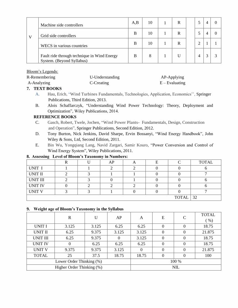
V
Machine side controllers A,B 10 1 R 5 4 0
Grid side controllers B 10 1 R 5 4 0
WECS in various countries B 10 1 R 2 1 1
Fault ride through technique in Wind Energy
System. (Beyond Syllabus)
B 8 1 U 4 3 3
Bloom’s Legends:
R-Remembering U-Understanding AP-Applying
A-Analyzing C-Creating E – Evaluating
7. TEXT BOOKS
A. Hau, Erich, “Wind Turbines Fundamentals, Technologies, Application, Economics’’, Springer
Publications, Third Edition, 2013.
B. Alois Schaffarczyk, “Understanding Wind Power Technology: Theory, Deployment and
Optimization”, Wiley Publications, 2014.
REFERENCE BOOKS
C. Gasch, Robert, Twele, Jochen, “Wind Power Plants- Fundamentals, Design, Construction
and Operation”, Springer Publications, Second Edition, 2012.
D. Tony Burton, Nick Jenkins, David Sharpe, Ervin Bossanyi, “Wind Energy Handbook”, John
Wiley & Sons, Ltd, Second Edition, 2011.
E. Bin Wu, Yongqiang Lang, Navid Zargari, Samir Kouro, “Power Conversion and Control of
Wind Energy System”, Wiley Publications, 2011.
8. Assessing Level of Bloom’s Taxonomy in Numbers:
R U AP A E C TOTAL
UNIT I 1 1 2 2 0 0 6
UNIT II 2 3 1 1 0 0 7
UNIT III 2 3 0 1 0 0 6
UNIT IV 0 2 2 2 0 0 6
UNIT V 3 3 1 0 0 0 7
TOTAL 32
9. Weight age of Bloom’s Taxonomy in the Syllabus
R U AP A E C TOTAL
( %)
UNIT I 3.125 3.125 6.25 6.25 0 0 18.75
UNIT II 6.25 9.375 3.125 3.125 0 0 21.875
UNIT III 6.25 9.375 0 3.125 0 0 18.75
UNIT IV 0 6.25 6.25 6.25 0 0 18.75
UNIT V 9.375 9.375 3.125 0 0 0 21.875
TOTAL 25 37.5 18.75 18.75 0 0 100
Lower Order Thinking (%) 100 %
Higher Order Thinking (%) NIL

10. Expected outcome of the course:
Upon successful completion of this course, the student will be able to:
CO1: Understand the importance of Wind Energy Conversion Systems.
CO2: Analyze the types of wind turbines.
CO3: Acquire the knowledge in various generator models.
CO4: Analyze the variable speed systems in wind energy systems.
CO5: Examine the concepts in grid connected system.
11. Mapping course outcome with Bloom’s Taxonomy LOT and HOT:
R U AP A E C
CO1 √ √ √
CO2 √ √
CO3 √√ √
CO4 √ √
CO5 √ √
12. Mapping Course outcome with graduate attributes:
GA1 GA2 GA3 GA4 GA5 GA6 GA7 GA8 GA9 GA10 GA11 GA12
CO1 √√ √ √ √
CO2 √√ √√ √ √ √
CO3 √√ √ √ √ √
CO4 √√ √ √√
CO5
13. Mapping course outcome with programme outcomes:
PO1 PO2 PO3 PO4 PO5 PO6 PO7 PO8 PO9 PO10 PO11 PO12
CO1 √√ √√ √ √ √ √ √ √ √
CO2 √√ √ √ √ √
CO3 √√ √ √ √ √ √ √
CO4 √ √√ √ √ √
CO5 √ √ √ √ √ √ √ √
14. Mapping with Programme Educational Objectives:
PEO1 PEO2 PEO3 PEO4 PEO5
CO1 √√ √ √ √
CO2 √√ √ √ √
CO3 √ √√ √ √
CO4 √ √ √ √
CO5 √ √ √ √
√√ Strongly agreed √ Moderately agreed
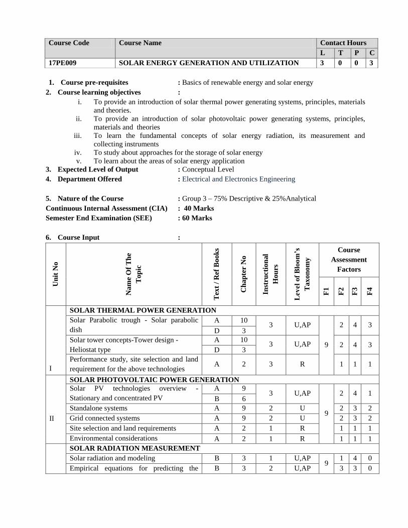
1. Course pre-requisites : Basics of renewable energy and solar energy
2. Course learning objectives :
i. To provide an introduction of solar thermal power generating systems, principles, materials
and theories.
ii. To provide an introduction of solar photovoltaic power generating systems, principles,
materials and theories
iii. To learn the fundamental concepts of solar energy radiation, its measurement and
collecting instruments
iv. To study about approaches for the storage of solar energy
v. To learn about the areas of solar energy application
3. Expected Level of Output : Conceptual Level
4. Department Offered : Electrical and Electronics Engineering
5. Nature of the Course : Group 3 – 75% Descriptive & 25%Analytical
Continuous Internal Assessment (CIA) : 40 Marks
Semester End Examination (SEE) : 60 Marks
6. Course Input :
Un
it N
o
Nam
e O
f T
he
Top
ic
Tex
t /
Ref
Book
s
Ch
ap
ter
No
Inst
ruct
ion
al
Hou
rs
Lev
el o
f B
loom
’s
Taxon
om
y
Course
Assessment
Factors
F1
F2
F3
F4
I
SOLAR THERMAL POWER GENERATION
Solar Parabolic trough - Solar parabolic
dish
A 10 3 U,AP
9
2 4 3 D 3
Solar tower concepts-Tower design -
Heliostat type
A 10 3 U,AP 2 4 3
D 3
Performance study, site selection and land
requirement for the above technologies A 2 3 R 1 1 1
II
SOLAR PHOTOVOLTAIC POWER GENERATION
Solar PV technologies overview -
Stationary and concentrated PV
A 9 3 U,AP
9
2 4 1 B 6
Standalone systems A 9 2 U 2 3 2
Grid connected systems A 9 2 U 2 3 2
Site selection and land requirements A 2 1 R 1 1 1
Environmental considerations A 2 1 R 1 1 1
SOLAR RADIATION MEASUREMENT
Solar radiation and modeling B 3 1 U,AP 9
1 4 0
Empirical equations for predicting the B 3 2 U,AP 3 3 0
Course Code Course Name Contact Hours
L T P C
17PE009 SOLAR ENERGY GENERATION AND UTILIZATION 3 0 0 3
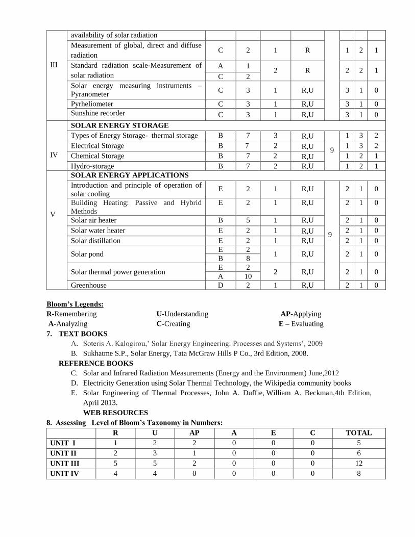
III
availability of solar radiation
Measurement of global, direct and diffuse
radiation C 2 1 R 1 2 1
Standard radiation scale-Measurement of
solar radiation
A 1 2 R 2 2 1
C 2
Solar energy measuring instruments –
Pyranometer C 3 1 R,U 3 1 0
Pyrheliometer C 3 1 R,U 3 1 0
Sunshine recorder C 3 1 R,U 3 1 0
IV
SOLAR ENERGY STORAGE
Types of Energy Storage- thermal storage B 7 3 R,U
9
1 3 2
Electrical Storage B 7 2 R,U 1 3 2
Chemical Storage B 7 2 R,U 1 2 1
Hydro-storage B 7 2 R,U 1 2 1
V
SOLAR ENERGY APPLICATIONS
Introduction and principle of operation of
solar cooling E 2 1 R,U
9
2 1 0
Building Heating: Passive and Hybrid
Methods
E 2 1 R,U 2 1 0
Solar air heater B 5 1 R,U 2 1 0
Solar water heater E 2 1 R,U 2 1 0
Solar distillation E 2 1 R,U 2 1 0
Solar pond E 2
1 R,U 2 1 0 B 8
Solar thermal power generation E 2
2 R,U 2 1 0 A 10
Greenhouse D 2 1 R,U 2 1 0
Bloom’s Legends:
R-Remembering U-Understanding AP-Applying
A-Analyzing C-Creating E – Evaluating
7. TEXT BOOKS
A. Soteris A. Kalogirou,’ Solar Energy Engineering: Processes and Systems’, 2009
B. Sukhatme S.P., Solar Energy, Tata McGraw Hills P Co., 3rd Edition, 2008.
REFERENCE BOOKS
C. Solar and Infrared Radiation Measurements (Energy and the Environment) June,2012
D. Electricity Generation using Solar Thermal Technology, the Wikipedia community books
E. Solar Engineering of Thermal Processes, John A. Duffie, William A. Beckman,4th Edition,
April 2013.
WEB RESOURCES
8. Assessing Level of Bloom’s Taxonomy in Numbers:
R U AP A E C TOTAL
UNIT I 1 2 2 0 0 0 5
UNIT II 2 3 1 0 0 0 6
UNIT III 5 5 2 0 0 0 12
UNIT IV 4 4 0 0 0 0 8

UNIT V 8 8 0 0 0 0 16
TOTAL 47
9. Weightage of Bloom’s Taxonomy in the Syllabus
R U AP A E C TOTAL
( %)
UNIT I 2.1 4.25 4.25 0 0 0 10.6
UNIT II 4.25 6.38 2.1 0 0 0 12.73
UNIT III 10.63 10.63 4.25 0 0 0 25.51
UNIT IV 8.51 8.51 0 0 0 0 17.02
UNIT V 17.02 17.02 0 0 0 0 34.04
TOTAL 42.51 46.72 10.6 0 0 0 100
Lower Order Thinking (%) 100 %
Higher Order Thinking (%) NIL
10. Expected outcome of the course:
Upon successful completion of this course, the student will be able:
CO1: To provide an introduction of solar thermal power generating systems, principles, materials and
theories.
CO2: To provide an introduction of solar photovoltaic power generating systems, principles, materials and
theories
CO3: To learn the fundamental concepts of solar energy radiation, its measurement and collecting
instruments
CO4: To study about approaches for the storage of solar energy
CO5: To learn about the areas of solar energy application
11. Mapping course outcome with Bloom’s Taxonomy LOT and HOT:
R U AP A E C
CO1 √ √
CO2 √ √
CO3 √ √
CO4 √ √
CO5 √√
12. Mapping Course outcome with graduate attributes:
GA1 GA2 GA3 GA4 GA5 GA6 GA7 GA8 GA9 GA10 GA11 GA12
CO1 √ √ √ √
CO2 √ √ √ √
CO3 √ √ √ √ √
CO4 √√ √ √√ √√ √
CO5 √√ √ √√ √√ √√ √√
13. Mapping course outcome with programme outcomes:
PO1 PO2 PO3 PO4 PO5 PO6 PO7 PO8 PO9 PO10 PO11 PO12
CO1 √ √ √ √ √
CO2 √ √ √ √ √

CO3 √ √√ √ √ √ √ √
CO4 √ √ √ √ √ √
CO5 √ √√ √√ √ √√ √ √√ √√ √
14. Mapping with Programme Educational Objectives:
PEO1 PEO2 PEO3 PEO4 PEO5
CO1 √ √
CO2 √ √
CO3 √ √ √
CO4 √ √
CO5 √√ √ √ √√
√√ Strongly agreed √ Moderately agreed

1. Course pre-requisites : Control system
2. Course learning objectives :
i. To expose the concepts of feed forward neural networks.
ii. To provide adequate knowledge about feed back neural networks.
iii. To teach about the concept of fuzziness involved in various systems.
iv. To expose the ideas about genetic algorithm
v. To provide adequate knowledge about of FLC and NN toolbox
3. Expected Level of Output : Conceptual Level
4. Department Offered : EEE
5. Nature of the Course : Group 3– 70 % Descriptive & 30% Analytical
Continuous Internal Assessment (CIA) : 40 Marks
Semester End Examination (SEE) : 60 Marks
6. Course Input :
Un
it N
o
Nam
e O
f T
he
Top
ic
Tex
t /
Ref
Book
s
Ch
ap
ter
No
Inst
ruct
ion
al
Hou
rs
Lev
el o
f B
loom
’s
Taxon
om
y
Course
Assessment
Factors
F1
F2
F3
F4
I
INTRODUCTION AND ARTIFICIAL NEURAL NETWORKS
Introduction of Soft Computing-Soft
computing vs hard computing-Various
types of soft computing techniques-
Applications of soft computing
A 1 2 U
9
5 5 3
Neuron-Nerve structure and Synapse-
Artificial Neuron and its model -
Activation functions - Neural network
architecture -Single layer and Multilayer
feed forward networks
A 1 3 U 5 5 2
McCullochPitts neuron model - Perceptron
model – Adaline and Madaline - Multilayer
perception model - Back propagation
learning methods
A 1 2 R 5 2 1
Effect of learning rule coefficient - back A 6 2 A 5 2 1
Course Code Course Name Contact Hours
L T P C
17PE010 SOFT COMPUTING TOOLS APPLIED IN ELECTRICAL
ENGINEERING
3 0 0 3

propagation algorithm - Factors affecting
Back propagation training - Applications
II
ARTIFICIAL NEURAL NETWORKS
Counter propagation network –
Architecture - Functioning &
Characteristics of counter -Propagation
Network
A 4 2 U
9
5 3 1
Hopfield/ Recurrent network –
Configuration - Stability constraints -
Associative memory and characteristics -
Limitations and applications - Hopfield v/s
Boltzmann machine
A 3 3 U 5 1 1
Adaptive Resonance Theory – Architecture
– Classifications A 5 2 U 5 1 1
Implementation and training - Associative
Memory A 3 2 AP 5 1 1
III
FUZZY LOGIC SYSTEM
Introduction to crisp sets and fuzzy sets -
Basic fuzzy set operation and approximate
reasoning
B 2 3 A
9
5 2 2
Introduction to fuzzy logic modeling and
control – Fuzzification – Inferencing and
defuzzification - Fuzzy knowledge and rule
bases - Fuzzy modeling and control
schemes for nonlinear systems
B 4 3 A 5 2 2
Self organizing fuzzy logic control - Fuzzy
logic control for nonlinear time delay
system
B 8 3 A 5 1 2
IV
GENETIC ALGORITHM
Basic concept of Genetic algorithm and
detail algorithmic steps - Adjustment of
free Parameters
D 1 3 A
9
3 1 1
Solution of typical control problems using
genetic algorithm D 3 3 U 3 1 1
Concept on some other search techniques
like Tabu Search and Ant Colony Search
techniques for solving optimization
problems
D 3 3 A 3 1 1
V
APPLICATIONS
GA application to power system
optimization problem - Case studies:
Identification and control of linear and
nonlinear dynamic systems using Matlab -
Neural Network toolbox
D 6 3 AP
9
5 2 0
Stability analysis of Neural Network
interconnection systems A 5 1 AP 5 2 0
Implementation of fuzzy logic controller
using Matlab Fuzzy logic toolbox -
Stability analysis of fuzzy control systems
B 13 5 AP 5 2 0

Bloom’s Legends:
R-Remembering U-Understanding AP-Applying
A-Analyzing C-Creating E – Evaluating
7. REFERENCE BOOKS
A. Laurene V. Fausett, Fundamentals of Neural Networks: Architectures, Algorithms and
Applications, Pearson Education, 2012.
B. Timothy J. Ross, “Fuzzy Logic with Engineering Applications” Wiley India, 2009.
C. Zimmermann H.J. "Fuzzy set theory and its Applications" Springer international edition, 2011.
D. David E.Goldberg, “Genetic Algorithms in Search, Optimization, and Machine Learning”,
Pearson Education, 2009
E. W.T.Miller, R.S.Sutton and P.J.Webrose, “Neural Networks for Control”, MIT Press, 1996.
WEB RESOURCES
8. Assessing Level of Bloom’s Taxonomy in Numbers:
R U AP A E C TOTAL
UNIT I 1 2 0 1 0 0 4
UNIT II 0 3 1 0 0 0 4
UNIT III 0 0 0 3 0 0 3
UNIT IV 0 1 0 2 0 0 3
UNIT V 0 0 3 0 0 0 3
TOTAL 17
9. Weight age of Bloom’s Taxonomy in the Syllabus
R U AP A E C TOTAL
( %)
UNIT I 5.88 11.76 0 5.88 0 0 23.52
UNIT II 0 17.64 5.88 0 0 0 23.52
UNIT III 0 0 0 17.64 0 0 17.64
UNIT IV 0 5.88 0 11.76 0 0 17.64
UNIT V 0 0 17.64 0 0 0 17.64
TOTAL 5.88 35.28 23.52 35.28 0 0 100
Lower Order Thinking (%) 64.68%
Higher Order Thinking (%) 35.28%
10. Expected outcome of the course:
Upon successful completion of this course, the student will be able to:
CO1: Understand the concepts of feed forward neural networks.
CO2: Understand about feedback neural networks.
CO3: Understand about the concept of fuzziness involved in various systems.
CO4: Understand ideas about genetic algorithm.
CO5: Understand about FLC and NN toolbox.
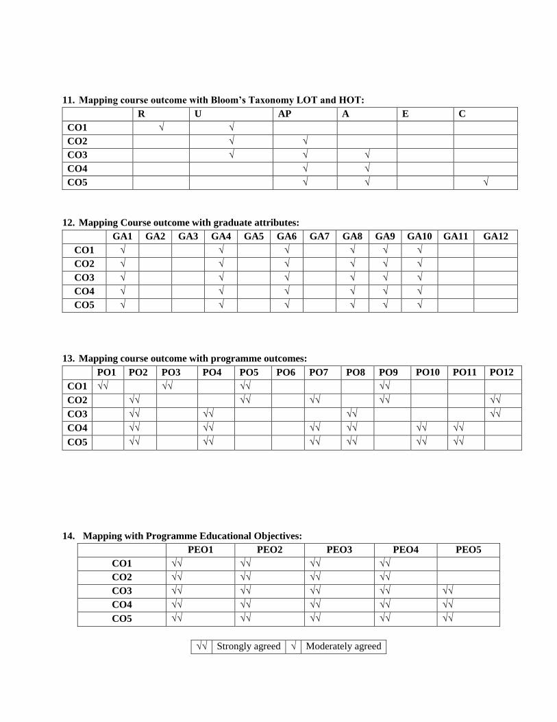
11. Mapping course outcome with Bloom’s Taxonomy LOT and HOT:
R U AP A E C
CO1 √ √
CO2 √ √
CO3 √ √ √
CO4 √ √
CO5 √ √ √
12. Mapping Course outcome with graduate attributes:
GA1 GA2 GA3 GA4 GA5 GA6 GA7 GA8 GA9 GA10 GA11 GA12
CO1 √ √ √ √ √ √
CO2 √ √ √ √ √ √
CO3 √ √ √ √ √ √
CO4 √ √ √ √ √ √
CO5 √ √ √ √ √ √
13. Mapping course outcome with programme outcomes:
PO1 PO2 PO3 PO4 PO5 PO6 PO7 PO8 PO9 PO10 PO11 PO12
CO1 √√ √√ √√ √√
CO2 √√ √√ √√ √√ √√
CO3 √√ √√ √√ √√
CO4 √√ √√ √√ √√ √√ √√
CO5 √√ √√ √√ √√ √√ √√
14. Mapping with Programme Educational Objectives:
PEO1 PEO2 PEO3 PEO4 PEO5
CO1 √√ √√ √√ √√
CO2 √√ √√ √√ √√
CO3 √√ √√ √√ √√ √√
CO4 √√ √√ √√ √√ √√
CO5 √√ √√ √√ √√ √√
√√ Strongly agreed √ Moderately agreed

1. Course pre-requisites :NIL
2. Course learning objectives :
i. To learn the basics about PLC and SCADA.
ii. To have an idea about programming languages and program control functions.
iii. To learn the ladder logic programming using corresponding functions.
iv. To know the basics of SCADA and its hardware, software.
v. To have a knowledge about communication protocols in SCADA.
3. Expected Level of Output :Understanding and creating
4. Department Offered :Electrical and Electronics Engineering
5. Nature of the Course :C. Group 3 – 80% Descriptive & 20%Analytical
Continuous Internal Assessment (CIA) : 40 Marks
Semester End Examination (SEE) :60 Marks
6. Course Input :
Un
it N
o
Nam
e O
f T
he
Top
ic
Tex
t /
Ref
Book
s
Ch
ap
ter
No
Inst
ruct
ion
al
Hou
rs
Lev
el o
f B
loom
’s
Taxon
om
y
Course
Assessment
Factors
F1
F2
F3
F4
I
INTRODUCTION TO PROGRAMMABLE LOGIC CONTROLLERS
Definition and History of PLC –Parts of
PLC-Principle of operation- modifying the
operation
A,B 1,1 2 U
9
5 4 1
PLC Advantages and Disadvantages -
Manufacturing and assembly Processes B 1 2 R 5 4 1
Overall PLC System Architecture- PLC
CPU, Solid state Memory, the processor,
Input and Output Modules, Power supplies.
A,B 2,1 3 U 4 3 2
Programming Languages: Ladder Diagram,
Function Block Diagram, Instruction List,
Structured Text and Sequential Function
Charts
A,B 5,3 2 A 5 4 1
II
PROGRAMMING OF PLC
Basics:Relay-Type instructions, instruction
addressing, Branch instructions, internal
relay instructions, EXAMINE IF CLOSED
and EXAMINE IF OPEN instructions.
A 5 2 AP 9
5 5 0
Fundamentals of Logic, Timer and Counter A,B 4,7,8, 3 E 5 3 1
Course Code Course Name Contact Hours
L T P C
17PE011 PLC AND SCADA 3 0 0 3

Instructions 3
Arithmetic and Comparison Functions,
SKIP and MCR function, A,B
10,11
4 2 E 5 2 2
Sequencer and Shift Register instructions. A 12 2 A 5 2 2
III
NETWORKING OF PLCs
Levels of Industrial Control -Types of
Networking – Remote I/O Expansion - Cell
Control by PLC
B 7 3 R
9
5 5 2
PLC installation, troubleshooting and
maintenance A,B 13,8 2 U 5 4 0
Data acquisition System: Components and
its functions A 14 1 U 5 5 0
Networks Basics: Introduction to Field Bus
and Process Bus – Control Networks and
Device Networks – Ethernet
D 5,11,
15 3 U 5 5 2
IV
SCADA
Introduction- Brief history- Principles of
modern SCADA system C 1 3 R
9
4 4 0
SCADA Hardware – SCADA software-
system implementation C 2 2 U 5 4 2
Remote terminal units, the master station:
Local area network C 2 2 A 5 4 1
System reliability - Availability –
Communication architecture C 2 2 U 5 3 1
V
FUNCTIONS AND PROTOCOLS OF SCADA
The components of a SCADA system -
SCADA software package: Redundancy,
System response time, Expandability of the
system
C 3 2 U
9
5 4 1
Introduction to protocols - High level data
link control (HDLC) protocol - Error
detection - Distributed network protocol
C 3 2 U 5 4 1
New technologies in SCADA systems –
Ethernet - types of Ethernet- TCP/IP
protocols
C 3,5 2 A 4 4 2
Troubleshooting and Maintenance-
Specifications of system C 8,9 3 U 5 3 0
Bloom’s Legends:
R-Remembering U-Understanding AP-Applying
A-Analyzing C-Creating E – Evaluating
7. TEXT BOOKS
A. Frank D. Petruzella, Programmable Logic Controllers”, Tata McGraw-Hill, New Delhi,
2011.

B. John W. Webb and Ronald A. Reis, “Programmable logic controllers: Principles and
Applications”, Prentice Hall India, New Delhi, 2009.
C. David Bailey, Edwin Right, “Practical SCADA for Industry”, Newnes (Elsevier), Mumbai,
2003.
REFERENCE BOOKS
D. Sunit Kumar Sen, “Fieldbus and Networking in Process Automation”, CRC Press, 2014.
E. Peng Zhang, “Advanced Industrial Control Technology”, Elsevier, 2010.
F. William Bolton, “Programmable Logic Controllers”, Newnes, 2006.
WEB RESOURCES
8. Assessing Level of Bloom’s Taxonomy in Numbers:
R U AP A E C TOTAL
UNIT I 1 2 0 1 0 0 4
UNIT II 0 0 1 1 2 0 4
UNIT III 1 3 0 0 0 0 4
UNIT IV 1 2 0 1 0 0 4
UNIT V 0 3 0 1 0 0 4
TOTAL 20
9. Weightage of Bloom’s Taxonomy in the Syllabus
R U AP A E C TOTAL
( %)
UNIT I 5 10 0 5 0 0 20
UNIT II 0 0 5 5 10 0 20
UNIT III 5 15 0 0 0 0 20
UNIT IV 5 10 0 5 0 0 20
UNIT V 0 15 0 5 0 0 20
TOTAL 15 50 5 20 10 0 100
Lower Order Thinking (%) 70 %
Higher Order Thinking (%) 30%
10. Expected outcome of the course:
Upon successful completion of this course, the student will be able to:
CO1: To learn the basics of Programmable Logic Controller
CO2: To understand and execute the ladder logic programming
CO3: To understand the networking concepts of PLC
CO4: To learn about the hardware and software of SCADA
CO5: To know the new technologies in SCADA
11. Mapping course outcome with Bloom’s Taxonomy LOT and HOT:
R U AP A E C
CO1 √ √
CO2 √ √ √ √ √
CO3 √ √
CO4 √ √
CO5 √ √

12. Mapping Course outcome with graduate attributes:
GA1 GA2 GA3 GA4 GA5 GA6 GA7 GA8 GA9 GA10 GA11 GA12
CO1 √ √
CO2 √√ √√ √√ √ √ √ √√ √ √
CO3 √√ √ √ √ √ √ √ √ √
CO4 √ √ √ √
CO5 √ √ √ √ √ √
13. Mapping course outcome with programme outcomes:
PO1 PO2 PO3 PO4 PO5 PO6 PO7 PO8 PO9 PO10 PO11 PO12
CO1 √ √ √ √ √ √ √
CO2 √ √√ √√ √ √ √ √√ √ √ √ √ √
CO3 √ √ √ √ √ √ √ √ √
CO4 √ √ √ √ √
CO5 √ √ √ √ √ √ √
14. Mapping with Programme Educational Objectives:
PEO1 PEO2 PEO3 PEO4 PEO5
CO1 √
CO2 √√ √√ √ √
CO3 √√ √ √ √
CO4 √
CO5 √√ √ √ √ √
√√ Strongly agreed √ Moderately agreed
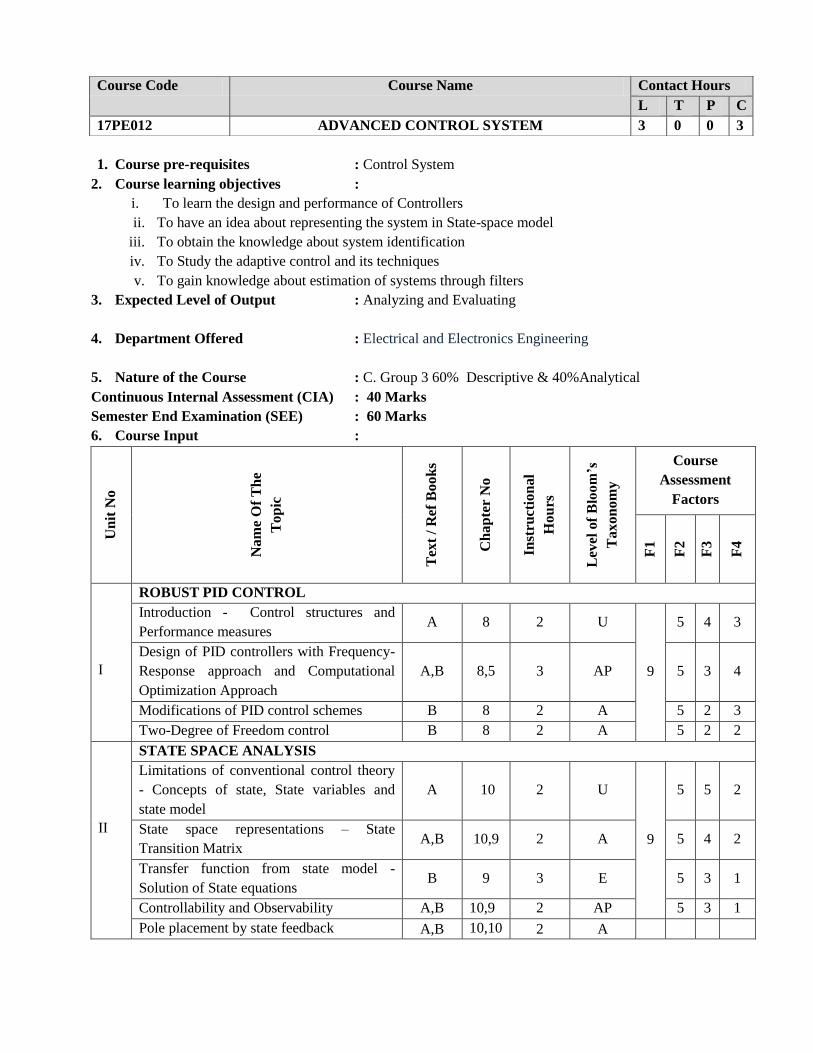
1. Course pre-requisites : Control System
2. Course learning objectives :
i. To learn the design and performance of Controllers
ii. To have an idea about representing the system in State-space model
iii. To obtain the knowledge about system identification
iv. To Study the adaptive control and its techniques
v. To gain knowledge about estimation of systems through filters
3. Expected Level of Output : Analyzing and Evaluating
4. Department Offered : Electrical and Electronics Engineering
5. Nature of the Course : C. Group 3 60% Descriptive & 40%Analytical
Continuous Internal Assessment (CIA) : 40 Marks
Semester End Examination (SEE) : 60 Marks
6. Course Input :
Un
it N
o
Nam
e O
f T
he
Top
ic
Tex
t /
Ref
Book
s
Ch
ap
ter
No
Inst
ruct
ion
al
Hou
rs
Lev
el o
f B
loom
’s
Taxon
om
y
Course
Assessment
Factors
F1
F2
F3
F4
I
ROBUST PID CONTROL
Introduction - Control structures and
Performance measures A 8 2 U
9
5 4 3
Design of PID controllers with Frequency-
Response approach and Computational
Optimization Approach
A,B 8,5 3 AP 5 3 4
Modifications of PID control schemes B 8 2 A 5 2 3
Two-Degree of Freedom control B 8 2 A 5 2 2
II
STATE SPACE ANALYSIS
Limitations of conventional control theory
- Concepts of state, State variables and
state model
A 10 2 U
9
5 5 2
State space representations – State
Transition Matrix A,B 10,9 2 A 5 4 2
Transfer function from state model -
Solution of State equations B 9 3 E 5 3 1
Controllability and Observability A,B 10,9 2 AP 5 3 1
Pole placement by state feedback A,B 10,10 2 A
Course Code Course Name Contact Hours
L T P C
17PE012 ADVANCED CONTROL SYSTEM 3 0 0 3

III
SYSTEM INDENTIFICATION
Models of LTI systems: Linear Models -
State space Models C 2 2 R
9
5 4 2
Output Error model - Model sets C 4 2 U 5 3 1
Structures and Identifiability C 5 2 U 5 3 2
Models for Time-varying and Non-linear
systems C,F 5 3 U 5 3 2
IV
ADAPTIVE COTROL
Introduction – Uses – Auto tuning – Self
Tuning Regulators (STR) D 3,4,8 2 U
9
5 3 1
Model Reference Adaptive Control
(MRAC) D 5 2 A 5 3 2
Types of STR and MRAC D 4,5 3 A 4 3 1
Different approaches to self tuning
regulators D 7,9 2 U 5 3 1
V
STATE ESTIMATION
Estimation of continuous linear systems E,I
1,
1,7 2 U
9
5 3 1
Wiener Hopf Integral equation J,I 4,16 3 A 5 3 1
Continuous Kalman filter E 2 2 U 5 3 1
Bloom’s Legends:
R-Remembering U-Understanding AP-Applying
A-Analyzing C-Creating E – Evaluating
7. TEXT BOOKS
A. Benjamin C Kuo, “Automatic Control Systems”, John Wiley & Sons, Inc., Delhi, 2010.
B. Katsuhiko Ogata, “Modern Control Engineering”, Pearson’s Education, Fifth Edition, New
Jersey, 2010.
C. Ljung L, “System Identification: Theory for the user”, Prentice Hall, New Jersey, 1999.
D. Astrom and Wittenmark,” Adaptive Control”, Dover Publications, 2008.
E. Arthur G O Mutambara, “Decentralized Estimation and Control for Multisensory Systems”,
CRC, 1998.
REFERENCE BOOKS F. GP RAO, L.Sivakumar, “Piecewise linear system identification via Walsh functions”,
International Journal of Systems Science, Vol.13, Iss 5, P.No 525-530, 1982.
G. Eykhoff P, “System Identification Parameter and State Estimation”, John Wiley and Sons,
London, 1974.
H. Narendra and Annasamy,” Stable Adaptive Control Systems”, Dover Publications, 2005.
I. Kailath T, Hassibi B and Sayed A H, “Linear Estimation”, Prentice Hall of India, New Delhi,
2000.
J. Arthur Gelb, “Applied Optimal Estimation”, The MIT Press, London, 2001.
WEB RESOURCES
K. http://nptel.ac.in/courses/108103007/
L. http://nptel.ac.in/courses/108101037/
8. Assessing Level of Bloom’s Taxonomy in Numbers:
R U AP A E C TOTAL
UNIT I 0 1 1 2 0 0 4

UNIT II 0 1 1 2 1 0 4
UNIT III 1 3 0 0 0 0 4
UNIT IV 0 2 0 2 0 0 4
UNIT V 0 2 0 1 0 0 4
TOTAL 20
9. Weightage of Bloom’s Taxonomy in the Syllabus
R U AP A E C TOTAL
( %)
UNIT I 0 5 5 10 0 0 20
UNIT II 0 5 5 10 5 0 20
UNIT III 5 15 0 0 0 0 20
UNIT IV 0 10 0 10 0 0 20
UNIT V 0 10 0 5 0 0 20
TOTAL 5 45 10 35 5 0 100
Lower Order Thinking (%) 60 %
Higher Order Thinking (%) 40%
10. Expected outcome of the course:
Upon successful completion of this course, the student will be able to:
CO1: To obtain the knowledge about controllers and its tuning methods
CO2: To get an idea about state space model and its analysis
CO3: To learn about model identification.
CO4: To learn about adaptive control techniques
CO5: To understand the concepts of optimal filters
11. Mapping course outcome with Bloom’s Taxonomy LOT and HOT:
R U AP A E C
CO1 √ √ √
CO2 √ √
CO3 √ √
CO4 √ √
CO5 √ √ √
12. Mapping Course outcome with graduate attributes:
GA1 GA2 GA3 GA4 GA5 GA6 GA7 GA8 GA9 GA10 GA11 GA12
CO1 √ √ √ √ √ √ √ √
CO2 √√ √√ √√ √ √ √ √ √ √ √
CO3 √ √ √ √ √ √ √ √
CO4 √ √ √ √ √ √
CO5 √ √ √ √ √ √ √ √ √ √
13. Mapping course outcome with programme outcomes:
PO1 PO2 PO3 PO4 PO5 PO6 PO7 PO8 PO9 PO10 PO11 PO12
CO1 √ √ √ √ √√ √ √ √ √√ √ √√ √
CO2 √ √√ √√ √ √ √ √

CO3 √ √ √ √ √ √
CO4 √ √ √ √ √ √ √
CO5 √ √ √ √√ √ √√ √ √√ √
14. Mapping withProgrammeEducational Objectives:
PEO1 PEO2 PEO3 PEO4 PEO5
CO1 √√ √ √ √√ √√
CO2 √ √√ √√
CO3 √ √
CO4 √ √ √
CO5 √√ √ √ √√ √√
√√ Strongly agreed √ Moderately agreed

1. Course pre-requisites : Machines, Power Electronics , Embedded Systems
2. Course learning objectives :
i. To study the Architecture of PIC 16C7X Microcontroller
ii. To understand the various peripherals of PIC 16C7X
iii. To study the C2XX DSP CPU and Instruction Set
iv. To understand the various peripherals of signal processors
v. To understand the applications of PIC and Signal Processors
3. Expected Level of Output : Conceptual Level
4. Department Offered : Electrical and Electronics Engineering
5. Nature of the Course : Group 3 – 75 % Descriptive & 25%Analytical
Continuous Internal Assessment (CIA) : 40 Marks
Semester End Examination (SEE) : 60 Marks
6. Course Input :
Un
it N
o
Nam
e O
f T
he
Top
ic
Tex
t /
Ref
Book
s
Ch
ap
ter
No
Inst
ruct
ion
al
Hou
rs
Lev
el o
f B
loom
’s
Taxon
om
y
Course
Assessment
Factors
F1
F2
F3
F4
I
PIC 16C7X MICROCONTROLLER
Architecture memory organization A 1 2 R
9
4 3 1
Addressing modes A 2 2 R 4 3 2
Instruction set A
2 2 U 4 2 3
Programming techniques simple programs A 2 3 U
3 2 2
II
PERIPHERALS OF PIC 16C7X
Timers , Interrupts A
6 3 AP
9
4 3 2
I/O ports , I 2C bus for peripheral chip
access
A 7,9 3 A
4 3 2
A/D converter , UART A
10,11 3 U 4 3 2
C2XX DSP CPU and Instruction Set
Course Code Course Name Contact Hours
L T P C
17PE013 EMBEDDED CONTROL OF ELECTRICAL DRIVES
3 0 0 3
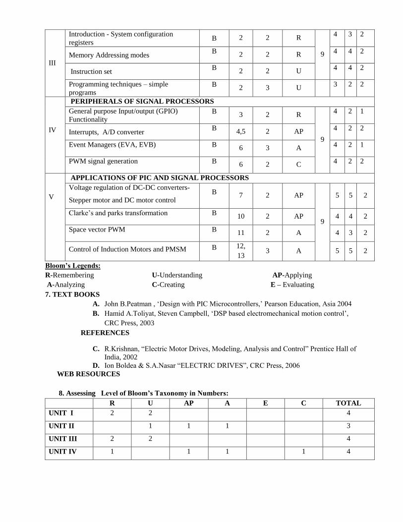
III
Introduction - System configuration
registers B 2 2 R
9
4 3 2
Memory Addressing modes B
2 2 R 4 4 2
Instruction set B
2 2 U 4 4 2
Programming techniques – simple
programs B 2 3 U
3 2 2
IV
PERIPHERALS OF SIGNAL PROCESSORS
General purpose Input/output (GPIO)
Functionality B
3 2 R
9
4 2 1
Interrupts, A/D converter B
4,5 2 AP 4 2 2
Event Managers (EVA, EVB) B 6 3 A 4 2 1
PWM signal generation B 6 2 C
4 2 2
V
APPLICATIONS OF PIC AND SIGNAL PROCESSORS
Voltage regulation of DC-DC converters-
Stepper motor and DC motor control B
7 2 AP
9
5 5 2
Clarke’s and parks transformation B 10 2 AP 4 4 2
Space vector PWM B 11 2 A 4 3 2
Control of Induction Motors and PMSM B 12,
13 3 A 5 5 2
Bloom’s Legends:
R-Remembering U-Understanding AP-Applying
A-Analyzing C-Creating E – Evaluating
7. TEXT BOOKS
A. John B.Peatman , ‘Design with PIC Microcontrollers,’ Pearson Education, Asia 2004
B. Hamid A.Toliyat, Steven Campbell, ‘DSP based electromechanical motion control’,
CRC Press, 2003
REFERENCES
C. R.Krishnan, “Electric Motor Drives, Modeling, Analysis and Control” Prentice Hall of
India, 2002
D. Ion Boldea & S.A.Nasar “ELECTRIC DRIVES”, CRC Press, 2006
WEB RESOURCES
8. Assessing Level of Bloom’s Taxonomy in Numbers:
R U AP A E C TOTAL
UNIT I 2 2 4
UNIT II 1 1 1 3
UNIT III 2 2 4
UNIT IV 1 1 1 1 4
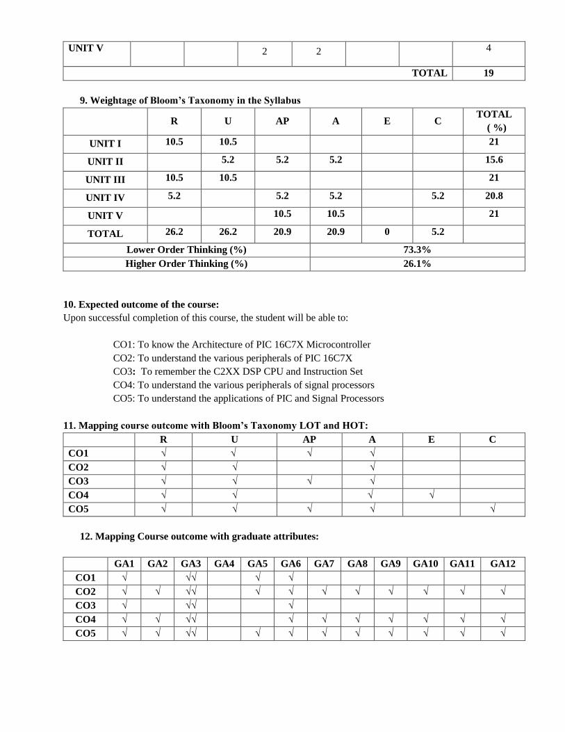
UNIT V 2 2 4
TOTAL 19
9. Weightage of Bloom’s Taxonomy in the Syllabus
R U AP A E C TOTAL
( %)
UNIT I 10.5 10.5 21
UNIT II 5.2 5.2 5.2 15.6
UNIT III 10.5 10.5 21
UNIT IV 5.2 5.2 5.2 5.2 20.8
UNIT V 10.5 10.5 21
TOTAL 26.2 26.2 20.9 20.9 0 5.2
Lower Order Thinking (%) 73.3%
Higher Order Thinking (%) 26.1%
10. Expected outcome of the course:
Upon successful completion of this course, the student will be able to:
CO1: To know the Architecture of PIC 16C7X Microcontroller
CO2: To understand the various peripherals of PIC 16C7X
CO3: To remember the C2XX DSP CPU and Instruction Set
CO4: To understand the various peripherals of signal processors
CO5: To understand the applications of PIC and Signal Processors
11. Mapping course outcome with Bloom’s Taxonomy LOT and HOT:
R U AP A E C
CO1 √ √ √ √
CO2 √ √ √
CO3 √ √ √ √
CO4 √ √ √ √
CO5 √ √ √ √ √
12. Mapping Course outcome with graduate attributes:
GA1 GA2 GA3 GA4 GA5 GA6 GA7 GA8 GA9 GA10 GA11 GA12
CO1 √ √√ √ √
CO2 √ √ √√ √ √ √ √ √ √ √ √
CO3 √ √√ √
CO4 √ √ √√ √ √ √ √ √ √ √
CO5 √ √ √√ √ √ √ √ √ √ √ √

13. Mapping course outcome with programme outcomes:
PO1 PO2 PO3 PO4 PO5 PO6 PO7 PO8 PO9 PO10 PO11 PO12
CO1 √√ √√ √√ √ √
CO2 √√ √√ √√ √ √ √√ √ √
CO3 √√ √√ √√ √ √
CO4 √√ √√ √√ √ √ √√ √ √
CO5 √√ √√ √√ √ √ √√ √ √
15. Mapping with Programme Educational Objectives:
PEO1 PEO2 PEO3 PEO4 PEO5
CO1 √√ √√
CO2 √√ √√ √√
CO3 √√ √√
CO4 √√ √√ √√
CO5 √√ √√ √ √√ √
√√ Strongly agreed √ Moderately agreed

1. Course pre-requisites : 11UBK651 - Digital Signal Processing
2. Course learning objectives :
i. Introduce to advanced DSP and MATLAB.
ii. To help students to understand the Estimation of spectrum analysis.
iii. To understand various design strategies of FIR and IIR filter.
iv. To introduce the concepts of wavelet based signal processing.
v. To help students to apply real time applications.
3. Expected Level of Output : Realistic Level
4. Department Offered : Electrical and Electronics Engineering
5. Nature of the Course : C. Group 3 –50% Descriptive & 50%Analytical
Continuous Internal Assessment (CIA) : 40 Marks
Semester End Examination (SEE) : 60 Marks
6. Course Input :
Un
it N
o
Nam
e O
f T
he
Top
ic
Tex
t /
Ref
Book
s
Ch
ap
ter
No
Inst
ruct
ion
al
Hou
rs
Lev
el o
f B
loom
’s
Taxon
om
y
Course
Assessment
Factors
F1
F2
F3
F4
I
INTRODUCTION TO DSP AND MATLAB
Sampling and representation of discrete
signals and systems. A,B 5,9 3 U
9
3 2 5
Amplitude and time quantization &
Difference equations A,B 5,9 2 R 2 1 4
Impulse, frequency and phase
responses A,B 5,9 2 R 3 1 3
Introduction to DSP simulation
software on the PC (MATLAB) A,B 5,1 2 U,E 5 5 4
II
SPECTRUM ESTIMATION
Estimation of spectra from finite
duration signals – Non-Parametric
Methods – Correlation Method
B,C,D 5,6 3 R
11
2 2 3
Periodogram Estimator – Performance
Analysis of Estimators – Unbiased, B,C,D 5,6 2 R 3 1 3
Course Code Course Name Contact Hours
L T P C
17PE014 DIGITAL SIGNAL PROCESSING USING MATLAB AND
WAVELETS
3 0 0 3

Consistent Estimators
Modified Periodogram – Bartlett and
Welch methods – Blackman – Tukey
method - Parametric Methods
B,C,D 6,7 3 R 3 2 3
AR, MA, and ARMA model based
spectral estimation – Parameter
Estimation –Yule-Walker equations –
Solutions using Durbins algorithm
B,C,D 6,7 3 R 3 2 3
III
DIGITAL FILTERS
FIR and IIR digital filter structures -
Properties A,B,F 3,6 3 U
8
4 4 4
Overview of some design techniques
for digital filters A,B,F 3,7 3 U 5 4 4
Frequency transformations from
prototype filters & Sources of error in
filter design
A,B,F 3,8 2 U,A 4 4 4
IV
WAVELET BASED SIGNAL PROCESSING
Introduction of wavelet transform,
uncertainty, wavelet analysis A 9 3 U,A
9
4 2 3
Multiresolution analysis A 9 1 U 3 2 3
Continuous wavelet transform –
Properties - Mother wavelet –
Redundancy
A 9 3 U,A 4 3 3
Discrete wavelet transform – Frequency
domain – Subband coding – Matrix
interpretation
A 9 2 U 4 3 4
V
APPLICATIONS
Image compression, Image
segmentation, Noise reduction &
Discontinuity detection in ECG signal
A 10 3 AP,E
8
5 3 3
Performing the 2D Discrete Wavelet
Transform on an image A 10 2 AP,E 5 4 2
Wavelet Transform with Matrices -
Filter Design A 10 2 AP,E 5 4 2
Frequency Magnitude Response of
Sound A 10 1 AP,E 5 2 3
Bloom’s Legends:
R-Remembering U-Understanding AP-Applying
A-Analyzing C-Creating E – Evaluating

7. TEXT BOOKS
A. Micheal weeks., digital signal processing using matlab with wavelets, george state
university, 2007.
B. Vinay k ingle.john g proakis., essentials of digital signal processing using matlab,
cengage learning, 2012.
REFERENCE BOOKS
C. Monson H. Hayes, Statistical Digital Signal Processing and Modeling, New Jersey,
John Wiley and Sons, 2002.
D. John G. Proakis and Dimitris G. Manolakis, Digital Signal Processing, New Delhi,
Pearson Education, 2002.
E. John G. Proakis, Algorithms for Statistical Signal Processing, New Delhi, Pearson
Education, 2002.
F. Robert j.shilling., Sandra l.harris., fundamentals of digital signal processing using
matlab, USA, cengage learning, 2010.
WEB RESOURCES
8. Assessing Level of Bloom’s Taxonomy in Numbers:
R U AP A E C TOTAL
UNIT I 2 2 0 0 1 0 5
UNIT II 4 0 0 0 0 0 4
UNIT III 0 3 0 1 0 0 4
UNIT IV 0 4 0 2 0 0 6
UNIT V 0 0 4 0 4 0 8
TOTAL 27
9. Weight age of Bloom’s Taxonomy in the Syllabus
R U AP A E C TOTAL
( %)
UNIT I 7.41 7.41 0 0 3.70 0 18.52 UNIT II 14.81 0 0 0 0 0 14.81
UNIT III 0 11.11 0 3.70 0 0 14.81
UNIT IV 0 14.81 0 7.41 0 0 22.22 UNIT V 0 0 14.81 0 14.81 0 29.62 TOTAL 22.22 33.33 14.81 11.11 18.51 0 100
Lower Order Thinking (%) 70 %
Higher Order Thinking (%) 30 %
10. Expected outcome of the course:
Upon successful completion of this course, the student will be able to:
CO1: Understand and remember the concept of DSP and MATLAB.
CO2: Students will be able to design System for estimation, Spectral Estimation and also able to
perform wave formation Analysis of the System
CO3: optimize & matched filters for best performance.
CO4: Understand the different wavelet transforms.
CO5: use MATLAB real time applications & to write small programs in MATLAB

11. Mapping course outcome with Bloom’s Taxonomy LOT and HOT:
R U AP A E C
CO1 √√ √√ √
CO2 √√
CO3 √√ √
CO4 √√ √
CO5 √√ √√
12. Mapping Course outcome with graduate attributes:
GA1 GA2 GA3 GA4 GA5 GA6 GA7 GA8 GA9 GA10 GA11 GA12
CO1 √√ √ √ √ √
CO2 √ √√ √
CO3 √ √ √√ √
CO4 √ √ √ √√
CO5 √ √ √√ √
13. Mapping course outcome with programme outcomes:
PO1 PO2 PO3 PO4 PO5 PO6 PO7 PO8 PO9 PO10 PO11 PO12
CO1 √√ √ √
CO2 √ √√ √√ √ √
CO3 √ √√ √√ √ √
CO4 √ √√ √√ √ √
CO5 √√ √ √
14. Mapping with Programme Educational Objectives:
PEO1 PEO2 PEO3 PEO4 PEO5
CO1 √ √ √
CO2 √ √ √
CO3 √√ √
CO4 √√ √
CO5 √√ √√
√√ Strongly agreed √ Moderately agreed

1. Course pre-requisites : Communication Engineering, Embedded Systems
2. Course learning objectives :
i. To study issues related to the design and analysis of systems with real-time constraints.
ii. To learn the features of Real time OS.
iii. To study the various Uniprocessor and Multiprocessor scheduling mechanisms.
iv. To learn about various real time communication protocols.
v. To study the difference between traditional and real time databases
3. Expected Level of Output : Conceptual Level
4. Department Offered : Electrical and Electronics Engineering
5. Nature of the Course : Group 1 – 100 % Descriptive
Continuous Internal Assessment (CIA) : 40 Marks
Semester End Examination (SEE) : 60 Marks
6. Course Input :
Un
it N
o
Nam
e O
f T
he
Top
ic
Tex
t /
Ref
Book
s
Ch
ap
ter
No
Inst
ruct
ion
al
Hou
rs
Lev
el o
f B
loom
’s
Taxon
om
y
Course
Assessment
Factors
F1
F2
F3
F4
I
INTRODUCTION TO REAL-TIME COMPUTING
Introduction to real time computing -
Concepts
A,B 1 1 R
9
3 3 2
Example of real-time applications – Structure
of a real time system
A,B 1 2 AP
5 4 2
Characterization of real time systems and
tasks
A,B 2 3 A
4 4 2
Performance measures A 2 3 R 4 3 1
II
TASK ASSIGNMENT AND SCHEDULING
Task allocation algorithms, Time services A,B,C 3 2 U
9
4 3 1
Single-processor and Multiprocessor task
scheduling, Scheduling Mechanisms
Communication and Synchronization
A,B,C
3 3 U
4 3 2
Clock-driven and priority A,B,C 3 3 R 3 2 2
based scheduling algorithms, Fault tolerant
scheduling
A,B,C 3 1 A
3 2 2
Course Code Course Name Contact Hours
L T P C
17PE015 REAL TIME OPERATING SYSTEMS 3 0 0 3

III
REAL-TIME COMMUNICATION
Threads and Tasks ,Protocols A,B 6 1 U
9
5 4 3
Contention-based, token-based, polled bus,
deadline based protocol
A,B 6 3 R
4 4 2
Fault tolerant routing A,B 6,7 3 A 5 3 3
RTP and RTCP. A,B 6,7 2 U 4 4 2
IV
REAL-TIME DATABASES
Transaction priorities and aborts A 5 2 U
9
4 2 1
Concurrency control issues A 5 2 U 4 2 2
Scheduling algorithms A 3,5 2 R 4 3 1
Two-phase approach to improve
predictability
A 5 3 A
4 2 2
V
PROGRAMMING LANGUAGES AND TOOLS
Hierarchical decomposition A,C 4 2 U
9
3 2 1
Run-time error handling A,C 4 2 U 3 2 1
Overloading - Timing specification A,C 4 3 A 3 2 1
Recent trends and developments. A,C 4 2 R 3 3 1
Bloom’s Legends:
R-Remembering U-Understanding AP-Applying
A-Analyzing C-Creating E – Evaluating
7. TEXT BOOKS
A. C.M. Krishna, Kang G. Shin – “ Real Time Systems”, International Edition, McGraw Hill
Companies, Inc., New York, 2010
B. Raj Kamal “ Embedded computer systems”, Tata McGraw-Hill Education, 2008
REFERENCE BOOKS
C. Jane W.S. Liu, Real-Time Systems, Pearson Education India, 2000.
D. Philip A. Laplante and Seppo J. Ovaska, “Real-Time Systems Design and Analysis: Tools for
the Practitioner’’ IV Edition IEEE Press, Wiley. 2011.
E. Qing Li, Caroline Yao “Real-Time Systems Design and Analysis” John Wiley & Sons, 2004.
WEB RESOURCES
8. Assessing Level of Bloom’s Taxonomy in Numbers:
R U AP A E C TOTAL
UNIT I 2 0 1 1 0 0 4
UNIT II 1 2 0 1 0 0 4
UNIT III 1 2 0 1 0 0 4
UNIT IV 1 2 0 1 0 0 4
UNIT V 1 2 0 1 0 0 4
TOTAL 20

9. Weight age of Bloom’s Taxonomy in the Syllabus
R U AP A E C TOTAL
( %)
UNIT I 10 0 5 5 0 0 20
UNIT II 5 10 0 5 0 0 20
UNIT III 5 10 0 5 0 0 20
UNIT IV 5 10 0 5 0 0 20
UNIT V 5 10 0 5 0 0 20
TOTAL 30 40 5 25 0 0 100
Lower Order Thinking (%) 75 %
Higher Order Thinking (%) 25%
10. Expected outcome of the course:
Upon successful completion of this course, the student will be able to:
CO1: Knowledge about Schedulability analysis.
CO2: Ability to learn Real-time programming environments
CO3: Knowledge about real time communication and databases.
CO4: Ability to develop real time systems.
CO5: Knowledge about future trends and developments in programming languages
11. Mapping course outcome with Bloom’s Taxonomy LOT and HOT:
R U AP A E C
CO1 √ √ √
CO2 √√
CO3 √√ √√ √√ √
CO4 √√ √
CO5 √ √√
12. Mapping Course outcome with graduate attributes:
GA1 GA2 GA3 GA4 GA5 GA6 GA7 GA8 GA9 GA10 GA11 GA12
CO1 √√ √√ √ √√ √ √
CO2 √√ √√ √ √ √ √√ √ √ √
CO3 √√ √ √ √ √
CO4 √√ √ √√ √√
CO5 √ √ √
13. Mapping course outcome with programme outcomes:
PO1 PO2 PO3 PO4 PO5 PO6 PO7 PO8 PO9 PO10 PO11 PO12
CO1 √√ √√ √ √ √ √ √ √ √
CO2 √√ √√ √√ √ √√ √√ √ √
CO3 √√ √ √ √
CO4 √√ √ √√ √ √ √
CO5 √

14. Mapping with Programme Educational Objectives:
PEO1 PEO2 PEO3 PEO4 PEO5
CO1 √ √ √
CO2 √√ √√ √ √√
CO3 √√ √√ √√
CO4 √√ √√
CO5 √√ √ √
√√ Strongly agreed √ Moderately agreed

1. Course pre-requisites : Engineering Mathematics ,Control systems
2. Course learning objectives :
i. To acquaint engineering students with mathematical optimization methods
ii. To study about unconstrained optimization techniques
iii. To study about constrained optimization techniques
iv. Introduce methods that are used in modern control system for Engineering Applications
v. To introduce state of art techniques for solving practical optimization problems
3. Expected Level of Output : Conceptual Level
4. Department Offered : Electrical and Electronics Engineering
5. Nature of the Course : Group 3 – 70% Descriptive & 30%Analytical
Continuous Internal Assessment (CIA) : 40 Marks
Semester End Examination (SEE) : 60 Marks
6. Course Input :
Un
it N
o
Nam
e O
f T
he
Top
ic
Tex
t /
Ref
Book
s
Ch
ap
ter
No
Inst
ruct
ion
al
Hou
rs
Lev
el o
f B
loom
’s
Taxon
om
y
Course
Assessment
Factors
F1
F2
F3
F4
I
CLASSICAL OPTIMIZATION TECHNIQUES
Introduction- Single-Variable optimization A 2 1 R
9
4 4 2
Multivariable optimization with no
constraints A 2 1 R 5 5 3
Multivariable optimization with Equality
constraints
A 2 2 R 5 5 3
Multivariable optimization with inequality A
2 2 R 5 5 3
Convex Programming Problem A 2 1 U 5 5 3
Dynamic Programming & gradient method,
Calculus of variation
A 9 2 U 5 5 3
UNCONSTRAINED OPTIMIZATION TECHNIQUES
Introduction to Optimum design A 7 1 U
9 4 4 2
General principles of optimization A 7 1 U 3 3 3
Course Code Course Name Contact Hours
L T P C
17PE016 OPTIMIZATION TECHNIQUES 3 0 0 3

II
Problem formulation & their
classifications
A 7 1
A 5 5 4
Single variable and multivariable
optimization
A 7 2
A 4 4 3
Techniques of unconstrained
minimization
A 7 1
A 5 4 4
Golden section, Random, pattern and
gradient search methods
A 7 2
A 3 3 3
Interpolation methods A 7 1 A 4 3 2
III
CONSTRAINED OPTIMIZATION TECHNIQUES
Optimization with equality and
inequality constraints A 8 2 AP
9
5 4 3
Direct methods A 8 2
A 5 4 4
Indirect methods using penalty functions A 8 2
A 5 4 4
Lagrange Multipliers A 8 2 A 4 3 3
Geometric Programming A 8 1
A 3 3 3
IV
MULTI OBJECTIVE OPTIMIZATION
Weighted Sum of Squares method A 9 2 A
9
3 3 3
Epsilon constrains method A 9 2 A 4 3 3
Goal attainment A 9 2 A 5 4 3
Examples A 9 1 E 5 5 5
Introduction to Optimal control and
Dynamic optimization A 9 2 U 5 4 4
V
ADVANCED OPTIMIZATION TECHNIQUES
Multi stage Optimization A 12 2 A
9
4 4 4
Dynamic Programming A 12 1 A 5 4 4
Stochastic programming; Multi objective
optimization A
12 2 E 4 3 2
Genetic algorithms and Simulated
Annealing techniques A 12 2 E 5 4 4
Neural network & Fuzzy logic principles in
Optimization A
12 2 E 5 4 4
Bloom’s Legends:
R-Remembering U-Understanding AP-Applying
A-Analyzing C-Creating E – Evaluating
7. TEXT BOOKS
A. Engineering Optimization-Theory and Practice, Singiresu S. Rao, 3rd/e, New Age International
(P) Limited, Publishers, 2013.
B. Allen J.Wood , Bruce F.Wollenberg “Power Generation ,operation and control”, 3rd/e, John

Wiley and sons, 2014.
REFERENCE BOOKS
C. Kalyanmoy Deb, “ Optimization for engineering design: algorithms and examples”, New Delhi
Prentice Hall of India, 2012.
D. Singiresu S Rao, Engineering optimization: theory and practice, 3rd/e, New Delhi New Age
International Publishers, 2013.
WEB RESOURCES
8. Assessing Level of Bloom’s Taxonomy in Numbers:
R U AP A E C TOTAL
UNIT I 4 2 0 0 0 0 6
UNIT II 0 2 0 5 0 0 7
UNIT III 0 0 1 4 0 0 5
UNIT IV 0 1 0 3 1 0 5
UNIT V 0 0 0 2 3 0 5
TOTAL 28
9. Weight age of Bloom’s Taxonomy in the Syllabus
R U AP A E C TOTAL
( %)
UNIT I 14.28 7.14 0 0 0 0 21.42
UNIT II 0 7.14 0 17.86 0 0 25
UNIT III 0 0 3.57 14.28 0 0 17.85
UNIT IV 0 3.57 0 10.71 3.57 0 17.85
UNIT V 0 0 0 7.14 10.71 0 17.85
TOTAL 14.28 17.85 3.57 49.98 14.28 0 99.96
Lower Order Thinking (%) 35.70%
Higher Order Thinking (%) 64.26%
10. Expected outcome of the course:
On completion of the course the student will be able to
CO1: Solve practical Optimization problem in Engineering using both classical methods and soft computing
techniques.
CO2: apply knowledge on unconstrained optimization problems
CO3: apply knowledge on constrained optimization problems
CO4: an ability to apply knowledge of mathematics, science, and engineering
CO5: an ability to use the techniques, skills, and modern engineering tools necessary for
Engineering practice.
11. Mapping course outcome with Bloom’s Taxonomy LOT and HOT:
R U AP A E C
CO1 √
CO2 √ √
CO3 √
CO4 √
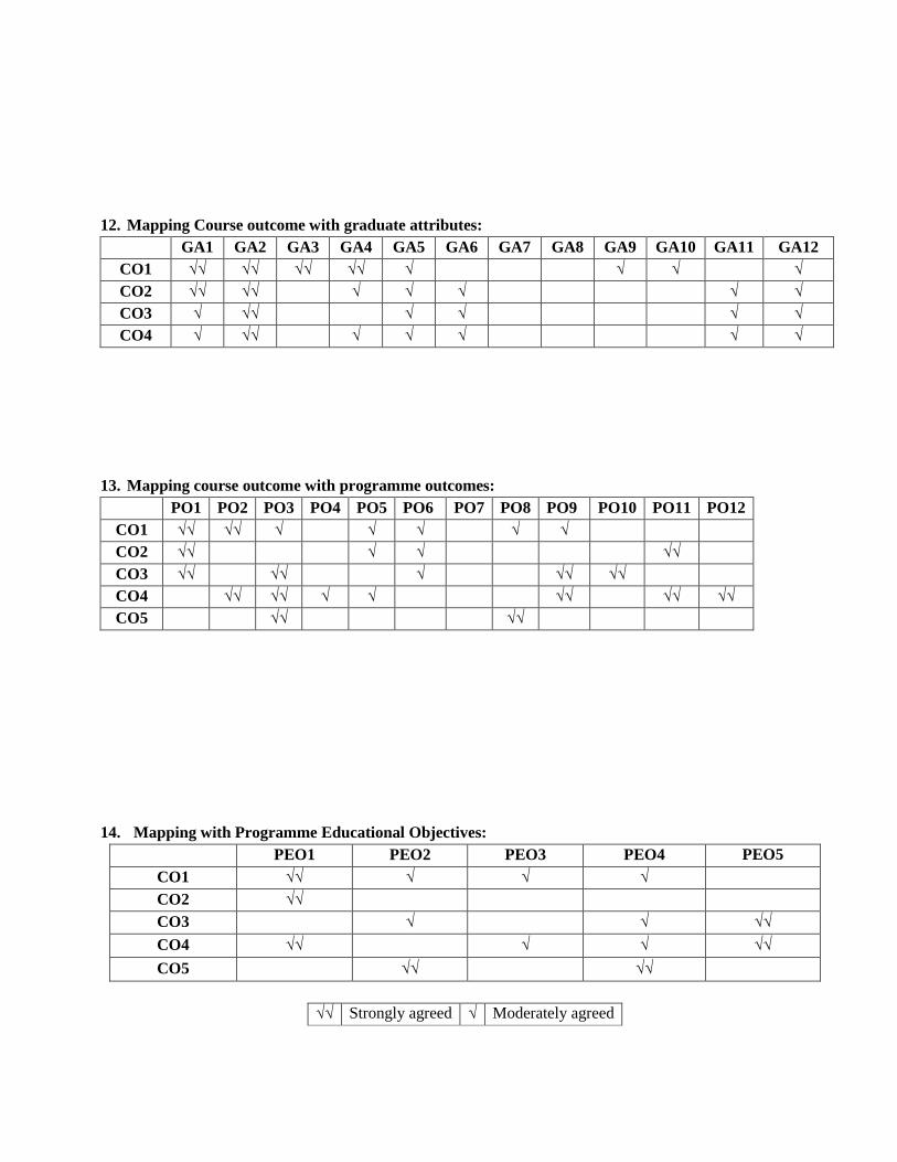
12. Mapping Course outcome with graduate attributes:
GA1 GA2 GA3 GA4 GA5 GA6 GA7 GA8 GA9 GA10 GA11 GA12
CO1 √√ √√ √√ √√ √ √ √ √
CO2 √√ √√ √ √ √ √ √
CO3 √ √√ √ √ √ √
CO4 √ √√ √ √ √ √ √
13. Mapping course outcome with programme outcomes:
PO1 PO2 PO3 PO4 PO5 PO6 PO7 PO8 PO9 PO10 PO11 PO12
CO1 √√ √√ √ √ √ √ √
CO2 √√ √ √ √√
CO3 √√ √√ √ √√ √√
CO4 √√ √√ √ √ √√ √√ √√
CO5 √√ √√
14. Mapping with Programme Educational Objectives:
PEO1 PEO2 PEO3 PEO4 PEO5
CO1 √√ √ √ √
CO2 √√
CO3 √ √ √√
CO4 √√ √ √ √√
CO5 √√ √√
√√ Strongly agreed √ Moderately agreed
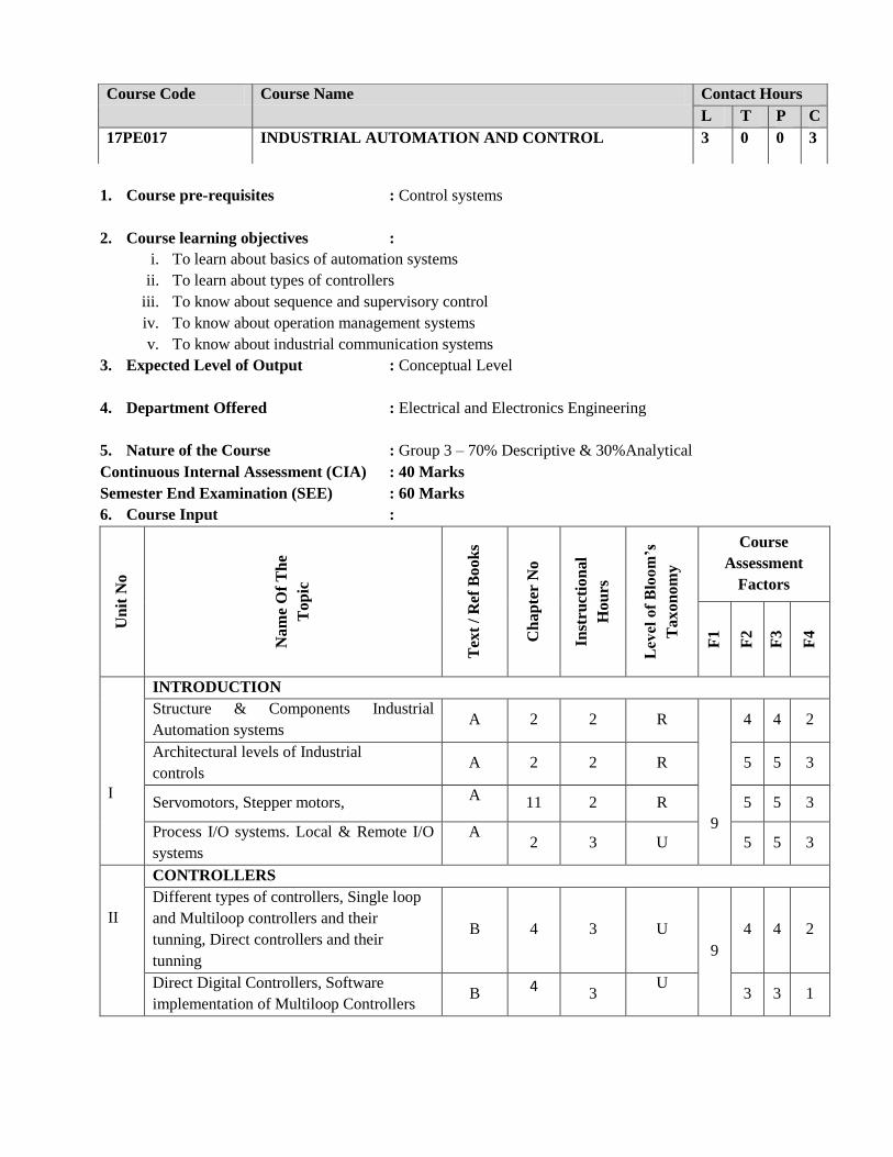
1. Course pre-requisites : Control systems
2. Course learning objectives :
i. To learn about basics of automation systems
ii. To learn about types of controllers
iii. To know about sequence and supervisory control
iv. To know about operation management systems
v. To know about industrial communication systems
3. Expected Level of Output : Conceptual Level
4. Department Offered : Electrical and Electronics Engineering
5. Nature of the Course : Group 3 – 70% Descriptive & 30%Analytical
Continuous Internal Assessment (CIA) : 40 Marks
Semester End Examination (SEE) : 60 Marks
6. Course Input :
Un
it N
o
Nam
e O
f T
he
Top
ic
Tex
t /
Ref
Book
s
Ch
ap
ter
No
Inst
ruct
ion
al
Hou
rs
Lev
el o
f B
loom
’s
Taxon
om
y
Course
Assessment
Factors
F1
F2
F3
F4
I
INTRODUCTION
Structure & Components Industrial
Automation systems A 2 2 R
9
4 4 2
Architectural levels of Industrial
controls A 2 2 R 5 5 3
Servomotors, Stepper motors, A
11 2 R 5 5 3
Process I/O systems. Local & Remote I/O
systems
A 2 3 U 5 5 3
II
CONTROLLERS
Different types of controllers, Single loop
and Multiloop controllers and their
tunning, Direct controllers and their
tunning
B 4 3 U
9
4 4 2
Direct Digital Controllers, Software
implementation of Multiloop Controllers B
4 3
U 3 3 1
Course Code Course Name Contact Hours
L T P C
17PE017 INDUSTRIAL AUTOMATION AND CONTROL 3 0 0 3

Distributed Control Systems B
4 3
A 4 2 2
III
SEQUENCE CONTROL & SUPERVISORY CONTROLLERS
Programmable Logic Controllers, Relay
Ladder Logic Programming B 2 2 U
9
4 3 2
Functionally of Supervisory Control Level B 3 2
AP 4 2 2
Process Optimization, Recipe
Management Material Tracking B 5 3
A 4 3 2
Man-machine interfaces B 5 2 A 4 3 2
IV
PROCESS OPERATION MANAGEMENT SYSTEMS
Overview of process operation
management systems order
A 13 3 AP
9
3 3 3
Inventory management A 13 3 AP 4 3 3
Process scheduling, quality management A 13 3 A 5 4 3
V
INDUSTRIAL COMMUNICATION SYSTEMS
Characteristic features of industrial
networks
A 16 3 AP
9
4 4 4
Low level networks
and their features, Field bus architecture
A 16 3 A 5 4 4
Performance aspects of Industrial
Automation Systems
A 16 3 A 4 3 2
Bloom’s Legends:
R-Remembering U-Understanding AP-Applying
A-Analyzing C-Creating E – Evaluating
7. TEXT BOOKS
A. Thomas E Kissell - Industrial electronics : applications for programmable controllers,
instrumentation and process control, and electrical machines and motor PHI learning
private limited 2009
B. George L Batten, Programmable controllers : hardware software and applications,
McGraw Hill Book Company,2009
REFERENCE BOOKS
C. Liptak B.G (ED)-Process Control H andbook,vol-2 Chilton book Co.
D. Noltinc - Handbook for Instrumentation Engineers.
E. Bollinger J.G and Duffie N.A-Computer control of machines and processes, Reading M A,
Addison-Wesley, 1988.
8. Assessing Level of Bloom’s Taxonomy in Numbers:
R U AP A E C TOTAL
UNIT I 3 1 4
UNIT II 2 1 3
UNIT III 1 1 2 4
UNIT IV 2 1 3
UNIT V 1 2 3
TOTAL 17

9. Weight age of Bloom’s Taxonomy in the Syllabus
R U AP A E C TOTAL
( %)
UNIT I 17.64 5.88 23.52
UNIT II 11.76 5.88 17.64
UNIT III 5.88 5.88 11.76 23.52
UNIT IV 11.76 5.88 17.64
UNIT V 5.88 11.76 17.64
TOTAL 17.64 23.52 23.52 35.28 99.96
Lower Order Thinking (%) 64.68%
Higher Order Thinking (%) 35.28%
10. Expected outcome of the course:
On completion of the course the student will be able to
CO1: know about basics of automation systems.
CO2: know about types of controllers
CO3: apply knowledge on Sequel and supervisory control
CO4: an ability to apply knowledge on operation management systems
CO5: an ability to apply knowledge on industrial communication systems
11. Mapping course outcome with Bloom’s Taxonomy LOT and HOT:
R U AP A E C
CO1 √
CO2 √ √
CO3 √
CO4 √
CO5 √ √
12. Mapping Course outcome with graduate attributes:
GA1 GA2 GA3 GA4 GA5 GA6 GA7 GA8 GA9 GA10 GA11 GA12
CO1 √√ √√ √√ √√ √ √ √ √
CO2 √√ √√ √ √ √ √ √
CO3 √ √√ √ √ √ √
CO4 √ √√ √ √ √ √ √
CO5 √√ √√ √√ √ √ √

13. Mapping course outcome with programme outcomes:
PO1 PO2 PO3 PO4 PO5 PO6 PO7 PO8 PO9 PO10 PO11 PO12
CO1 √√ √√ √ √ √ √ √
CO2 √√ √ √ √√
CO3 √√ √√ √ √√ √√
CO4 √√ √√ √ √ √√ √√ √√
CO5 √√ √√
14. Mapping with Programme Educational Objectives:
PEO1 PEO2 PEO3 PEO4 PEO5
CO1 √√ √ √ √
CO2 √√
CO3 √ √ √√
CO4 √√ √ √ √√
CO5 √√ √√
√√ Strongly agreed √ Moderately agreed
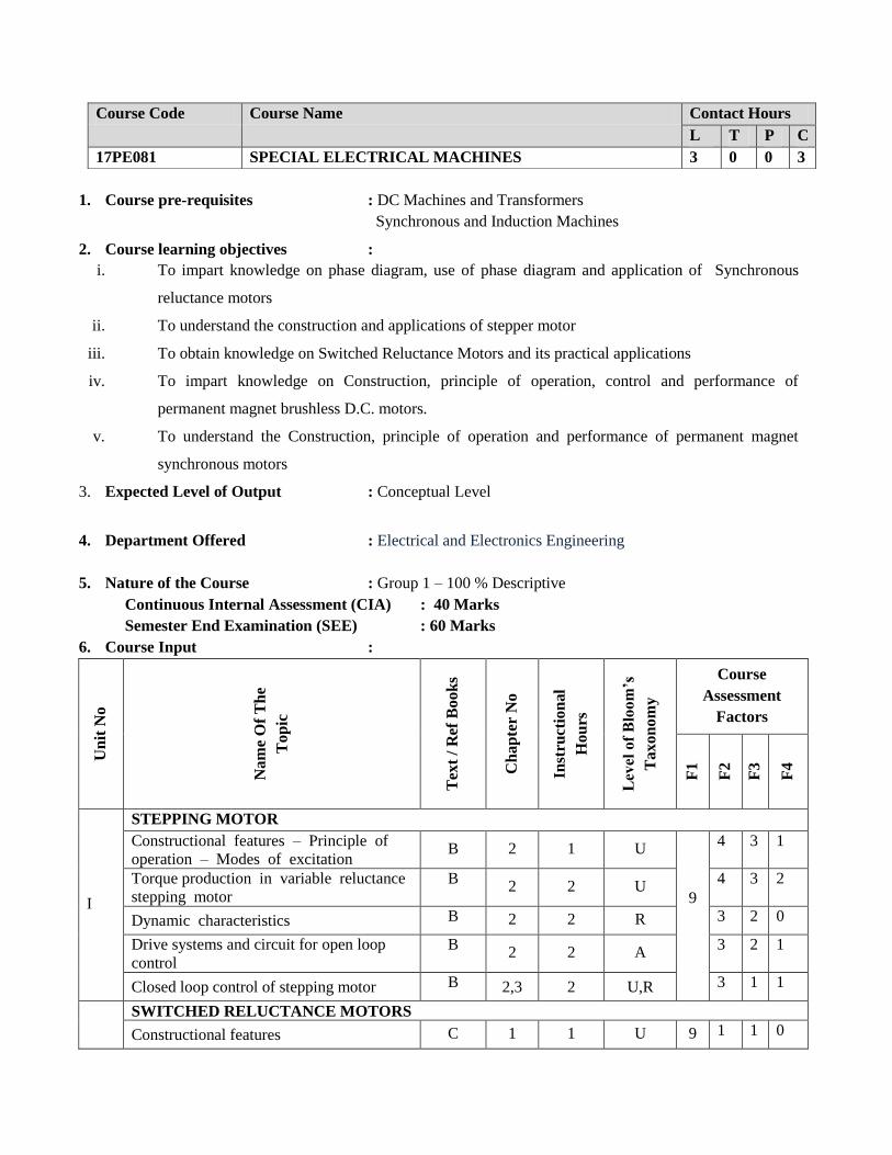
1. Course pre-requisites : DC Machines and Transformers
Synchronous and Induction Machines
2. Course learning objectives :
i. To impart knowledge on phase diagram, use of phase diagram and application of Synchronous
reluctance motors
ii. To understand the construction and applications of stepper motor
iii. To obtain knowledge on Switched Reluctance Motors and its practical applications
iv. To impart knowledge on Construction, principle of operation, control and performance of
permanent magnet brushless D.C. motors.
v. To understand the Construction, principle of operation and performance of permanent magnet
synchronous motors
3. Expected Level of Output : Conceptual Level
4. Department Offered : Electrical and Electronics Engineering
5. Nature of the Course : Group 1 – 100 % Descriptive
Continuous Internal Assessment (CIA) : 40 Marks
Semester End Examination (SEE) : 60 Marks
6. Course Input :
Un
it N
o
Nam
e O
f T
he
Top
ic
Tex
t /
Ref
Book
s
Ch
ap
ter
No
Inst
ruct
ion
al
Hou
rs
Lev
el o
f B
loom
’s
Taxon
om
y
Course
Assessment
Factors
F1
F2
F3
F4
I
STEPPING MOTOR
Constructional features – Principle of
operation – Modes of excitation B 2 1 U
9
4 3 1
Torque production in variable reluctance
stepping motor
B 2 2 U
4 3 2
Dynamic characteristics B 2 2 R 3 2 0
Drive systems and circuit for open loop
control
B 2 2 A
3 2 1
Closed loop control of stepping motor B 2,3 2 U,R 3 1 1
SWITCHED RELUCTANCE MOTORS
Constructional features C 1 1 U 9 1 1 0
Course Code Course Name Contact Hours
L T P C
17PE081 SPECIAL ELECTRICAL MACHINES 3 0 0 3

II
Principle of operation C 1 2 R 3 1 1
Torque equation C 2 1 A 2 2 0
Power controllers C 3,4 2 U 4 4 1
Characteristics C 4 1 R 5 3 1
Control microprocessor based controller C 8 1 U,R 5 5 5
III
SYNCHRONOUS RELUCTANCE MOTORS
Constructional features: axial and radial
air gap Motors A,C 2,3 2 R
9
3 3 2
Operating principle –Reluctance torque A,C 2,3 3 AP 5 4 2
Phasor diagram A,C 3,4 2 A 4 4 2
Motor characteristics A,C 3,4 2 R 4 3 1
IV
PERMANENT MAGNET SYNCHRONOUS MOTROS
Principle of operation –EMF A 6 2 U
9
4 2 1
Power input and torque expressions A 6 2 E 4 1 2
Phasor diagram –Power controller A 6 2 R 4 1 1
Torque speed characteristics-Self control A 6 1 A 4 1 2
Vector control –Current control schemes A 6 2 U 2 1 1
V
PERMANENT MAGNET BRUSHLESS DC MOTORS
Commutation in DC motors, Difference
between mechanical and electronic
commutators
A 5 2 U
9
5 5 2
Hall sensors, Optical sensors - Multiphase
Brushless motor A 5 2 E 4 4 2
Square wave permanent magnet brushless
motor drives –Torque and emf equation A 5 2 A 3 1 2
Torque speed characteristics-Controllers
Microprocessors based controller A 5 3 R,U 5 5 5
Bloom’s Legends:
R-Remembering U-Understanding AP-Applying
A-Analyzing C-Creating E – Evaluating
7. REFERENCES
A. Miller, T.J.E. “Brushless permanent magnet and reluctance motor drives”,Clarendon Press, Oxford,
1989.
B. Kenjo, T, “Stepping motors and their microprocessor control”, Clarendon Press, Oxford 1989.
C. R.Krishnan, “Switched Reluctance Motors Drives: Modelling, Simulation, Analysis Design and
Applications”, CRC Press, New York, 2001.

TEXT BOOKS
D. D.P.Kothari and I.J.Nagrath “Electric machines” Tata McGraw-Hill Education, 2010.
E. K. Venkataratnam “Special Electric Machines” Universities Press, 2009.
WEB RESOURCES
8. Assessing Level of Bloom’s Taxonomy in Numbers:
R U AP A E C TOTAL
UNIT I 2 3 0 1 0 0 6
UNIT II 3 3 0 1 0 0 7
UNIT III 2 0 1 1 0 0 4
UNIT IV 1 2 0 1 1 0 5
UNIT V 1 2 0 1 1 0 5
TOTAL 27
9. Weight age of Bloom’s Taxonomy in the Syllabus
R U AP A E C TOTAL
( %)
UNIT I 7.6 11.2 0 3.6 0 0 22.4
UNIT II 11.2 11.2 0 3.6 0 0 26
UNIT III 7.6 0 3.6 3.6 0 0 14.8
UNIT IV 3.6 7.6 0 3.6 3.6 0 18.4
UNIT V 3.6 7.6 0 3.6 3.6 0 18.4
TOTAL 33.7 37.7 3.6 17.8 7.2 0 100
Lower Order Thinking (%) 100 %
Higher Order Thinking (%) NIL
10. Expected outcome of the course:
Upon successful completion of this course, the student will be able to:
CO1. List the different motors and its properties
CO2. Understand the construction and working of different types of motor
CO3. Understand the phase diagrams and power controllers
CO4. Understand the application of motors
CO5. Understand the basic Principle of different types of motor
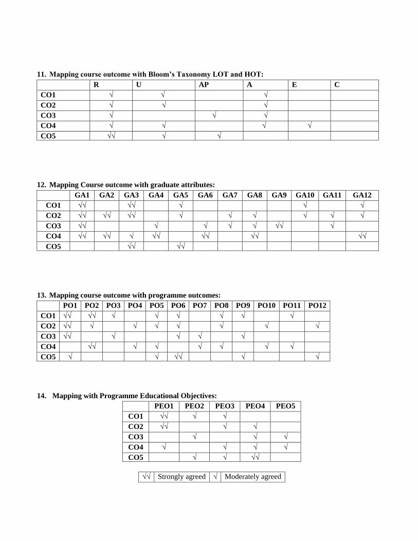
11. Mapping course outcome with Bloom’s Taxonomy LOT and HOT:
R U AP A E C
CO1 √ √ √
CO2 √ √ √
CO3 √ √ √
CO4 √ √ √ √
CO5 √√ √ √
12. Mapping Course outcome with graduate attributes:
GA1 GA2 GA3 GA4 GA5 GA6 GA7 GA8 GA9 GA10 GA11 GA12
CO1 √√ √√ √ √ √
CO2 √√ √√ √√ √ √ √ √ √ √
CO3 √√ √ √ √ √ √√ √
CO4 √√ √√ √ √√ √√ √√ √√
CO5 √√ √√
13. Mapping course outcome with programme outcomes:
PO1 PO2 PO3 PO4 PO5 PO6 PO7 PO8 PO9 PO10 PO11 PO12
CO1 √√ √√ √ √ √ √ √ √
CO2 √√ √ √ √ √ √ √ √
CO3 √√ √ √ √ √
CO4 √√ √ √ √ √ √ √
CO5 √ √ √√ √ √
14. Mapping with Programme Educational Objectives:
PEO1 PEO2 PEO3 PEO4 PEO5
CO1 √√ √ √
CO2 √√ √ √
CO3 √ √ √
CO4 √ √ √ √
CO5 √ √ √√
√√ Strongly agreed √ Moderately agreed
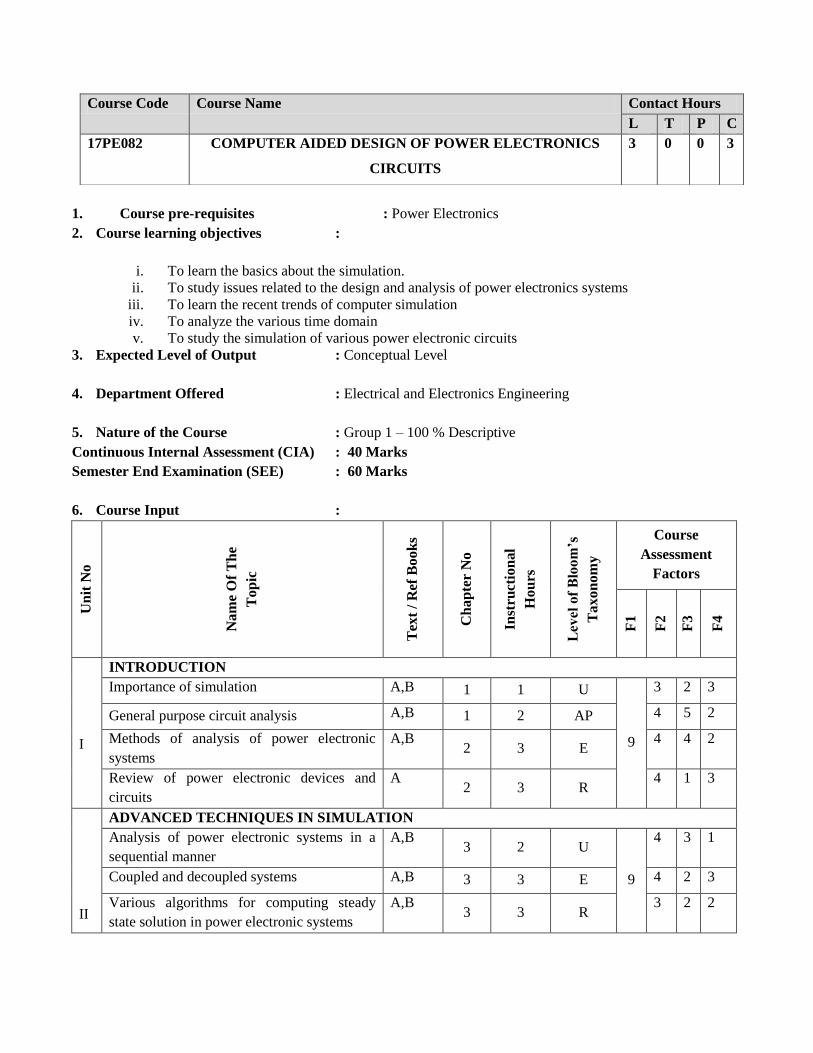
1. Course pre-requisites : Power Electronics
2. Course learning objectives :
i. To learn the basics about the simulation.
ii. To study issues related to the design and analysis of power electronics systems
iii. To learn the recent trends of computer simulation
iv. To analyze the various time domain
v. To study the simulation of various power electronic circuits
3. Expected Level of Output : Conceptual Level
4. Department Offered : Electrical and Electronics Engineering
5. Nature of the Course : Group 1 – 100 % Descriptive
Continuous Internal Assessment (CIA) : 40 Marks
Semester End Examination (SEE) : 60 Marks
6. Course Input :
Un
it N
o
Nam
e O
f T
he
Top
ic
Tex
t /
Ref
Book
s
Ch
ap
ter
No
Inst
ruct
ion
al
Hou
rs
Lev
el o
f B
loom
’s
Taxon
om
y
Course
Assessment
Factors
F1
F2
F3
F4
I
INTRODUCTION
Importance of simulation A,B 1 1 U
9
3 2 3
General purpose circuit analysis A,B 1 2 AP 4 5 2
Methods of analysis of power electronic
systems
A,B 2 3 E
4 4 2
Review of power electronic devices and
circuits
A 2 3 R
4 1 3
II
ADVANCED TECHNIQUES IN SIMULATION
Analysis of power electronic systems in a
sequential manner
A,B 3 2 U
9
4 3 1
Coupled and decoupled systems A,B 3 3 E 4 2 3
Various algorithms for computing steady
state solution in power electronic systems
A,B 3 3 R
3 2 2
Course Code Course Name Contact Hours
L T P C
17PE082 COMPUTER AIDED DESIGN OF POWER ELECTRONICS
CIRCUITS
3 0 0 3
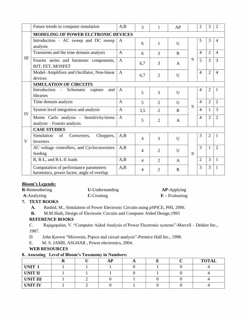
Future trends in computer simulation A,B 3 1 AP 2 3 2
III
MODELING OF POWER ELCTRONIC DEVICES
Introduction – AC sweep and DC sweep
analysis
A 6 1 U
9
5 3 4
Transients and the time domain analysis A 6 3 R 4 2 4
Fourier series and harmonic components,
BJT, FET, MOSFET
A 6,7 3 A
5 3 3
Model- Amplifiers and Oscillator, Non-linear
devices
A 6,7 2 U
4 2 4
IV
SIMULATION OF CIRCUITS
Introduction – Schematic capture and
libraries
A 5 3 U
9
4 2 1
Time domain analysis A 5 2 U 4 2 2
System level integration and analysis A 3,5 2 R 4 1 3
Monte Carlo analysis – Sensitivity/stress
analysis – Fourier analysis.
A 5 2 A
4 2 2
V
CASE STUDIES
Simulation of Converters, Choppers,
Inverters
A,B 4 3 U
9
3 2 1
AC voltage controllers, and Cycloconverters
feeding
A,B 4 2 U
3 1 2
R, R-L, and R-L-E loads A,B 4 2 A 2 3 1
Computation of performance parameters:
harmonics, power factor, angle of overlap
A,B 4 2 R
3 3 1
Bloom’s Legends:
R-Remembering U-Understanding AP-Applying
A-Analyzing C-Creating E – Evaluating
7. TEXT BOOKS
A. Rashid, M., Simulation of Power Electronic Circuits using pSPICE, PHI, 2006.
B. M.M.Shah, Design of Electronic Circuits and Computer Aided Design,1993
REFERENCE BOOKS
C. Rajagopalan, V. “Computer Aided Analysis of Power Electronic systems”-Marcell – Dekker Inc.,
1987.
D. John Keown “Microsim, Pspice and circuit analysis”-Prentice Hall Inc., 1998.
E. M. S. JAMIL ASGHAR , Power electronics, 2004.
WEB RESOURCES
8. Assessing Level of Bloom’s Taxonomy in Numbers:
R U AP A E C TOTAL
UNIT I 1 1 1 0 1 0 4
UNIT II 1 1 1 0 1 0 4
UNIT III 1 2 0 1 0 0 4
UNIT IV 1 2 0 1 0 0 4

UNIT V 1 2 0 1 0 0 4
TOTAL 20
9. Weight age of Bloom’s Taxonomy in the Syllabus
R U AP A E C TOTAL
( %)
UNIT I 5 5 5 0 5 0 20
UNIT II 5 5 5 0 5 0 20
UNIT III 5 10 0 5 0 0 20
UNIT IV 5 10 0 5 0 0 20
UNIT V 5 10 0 5 0 0 20
TOTAL 25 40 10 15 10 0 100
Lower Order Thinking (%) 75 %
Higher Order Thinking (%) 25%
10. Expected outcome of the course:
Upon successful completion of this course, the student will be able to:
CO1: Knowledge about time domain analysis.
CO2: Ability to learn future trends of computer simulation
CO3: Knowledge about power electronics circuits.
CO4: Ability to develop various power electronic circuits simulation.
CO5: Ability to develop a model for power electronic devices.
11. Mapping course outcome with Bloom’s Taxonomy LOT and HOT:
R U AP A E C
CO1 √ √ √ √√
CO2 √√
CO3 √ √ √√ √ √√
CO4 √√ √
CO5 √ √ √ √√ √√
12. Mapping Course outcome with graduate attributes:
GA1 GA2 GA3 GA4 GA5 GA6 GA7 GA8 GA9 GA10 GA11 GA12
CO1 √√ √√ √ √ √ √
CO2 √√ √ √ √ √ √√ √ √ √
CO3 √ √√ √ √ √ √
CO4 √ √ √√ √
CO5 √√ √ √ √ √ √√ √ √ √
13. Mapping course outcome with programme outcomes:
PO1 PO2 PO3 PO4 PO5 PO6 PO7 PO8 PO9 P10 P11 P12
CO1 √√ √√ √ √ √ √ √ √√ √
CO2 √√ √ √√ √√ √√ √√ √ √√
CO3 √√ √ √ √√
CO4 √√ √ √√ √ √ √
CO5 √√ √ √√ √√ √√ √√ √ √ √√
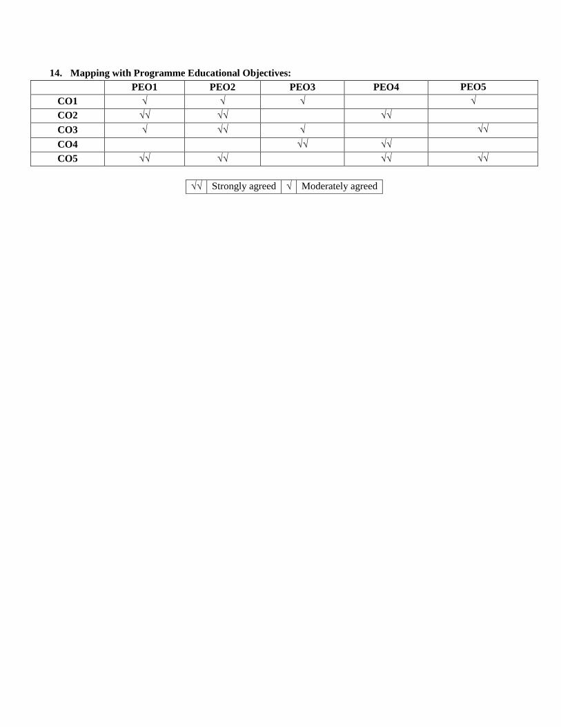
14. Mapping with Programme Educational Objectives:
PEO1 PEO2 PEO3 PEO4 PEO5
CO1 √ √ √ √
CO2 √√ √√ √√
CO3 √ √√ √ √√
CO4 √√ √√
CO5 √√ √√ √√ √√
√√ Strongly agreed √ Moderately agreed

1. Course pre-requisites :Basic electron devices
2. Course learning objectives :
i. To introduce MOS theory and manufacturing Technology.
ii. To study inverter, logic gates and stick diagrams for layout design
iii. To analyze the characteristics and performance of circuits.
iv. To understand the design of VLSI system components circuits.
v. To design digital circuits using Verilog HDL
3. Expected Level of Output :Conceptual Level
4. Department Offered :Electrical and Electronics Engineering
5. Nature of the Course :Group 1 – 100 % Descriptive
Continuous Internal Assessment (CIA) : 40 Marks
Semester End Examination (SEE) :60 Marks
6. Course Input :
Un
it N
o
Nam
e O
f T
he
Top
ic
Tex
t /
Ref
Book
s
Ch
ap
ter
No
Inst
ruct
ion
al
Hou
rs
Lev
el o
f B
loom
’s
Taxon
om
y
Course
Assessment
Factors
F1
F2
F3
F4
I
MOS TRANSISTOR THEORY AND PROCESS TECHNOLOGY
NMOS and PMOS transistors -Threshold
voltage , Body effect A 1 3 R&U
9
5 4 3
Design equations , Second order effects A 2 2 R&U 3 3 1
MOS models and small signal AC
characteristics A 2 2 U 1 0 0
Basic CMOS technology. A 3 2 U 2 0 0
II
INVERTERS AND LOGIC GATES
NMOS and CMOS Inverters, Stick
diagram, Inverter ratio B
2.6,
3.2 3 U&Ap
9
4 3 2
DC and transient characteristics ,
switching times, Super buffers B 3 2 U 2 0 1
Driving large capacitance loads, CMOS
logic structures, Transmission gates A 2 2 U 4 2 2
Course Code Course Name Contact Hours
L T P C
17PE083 VLSI DESIGN 3 0 0 3

Static CMOS design , Dynamic CMOS
design A 5 2 R&U 4 2 1
III
CIRCUIT CHARACTERISATION AND PERFORMANCE ESTIMATION
Resistance estimation, Capacitance
estimation & Inductance A
4.2-
4.4 3 U
9
1 0 1
Switching characteristics, Transistor sizing A 4.5 2 A 2 0 1
Power dissipation and design margining A 5 2 U 3 0 0
Charge sharing, Scaling. A 5 2 A 2 0 0
IV
VLSI SYSTEM COMPONENTS CIRCUITS
Multiplexers ,Decoders , comparators C
11.1-
11.3 2 C
9
4 0 0
Priority encoders , Shift registers C
11.4-
11.5 2 C 4 0 0
Arithmetic circuits -Ripple carry adders,
Carry look ahead adders C
12.1-
12.3 3 C 3 0 0
High-speed adders ,Multipliers C
12.4-
12.5 2 C 3 0 0
V
VERILOG HARDWARE DESCRIPTION LANGUAGE
Overview of digital design with Verilog
HDL D
1.1-
1.6 2 Ap
9
3 0 0
Hierarchical modeling concepts D
2.1-
2.7 2 Ap 3 0 0
Modules and port Definitions. Gate level
Modeling D
4.1-
4.2,5 2 Ap 3 0 0
Data flow modeling - Behavioral modeling D 6-7 3 Ap 3 0 0
Bloom’s Legends:
R-Remembering U-Understanding AP-Applying
A-Analyzing C-Creating E – Evaluating
7. TEXT BOOKS
A. Neil H E Weste; David Harris; Ayan Banerjee,”CMOS VLSI design: a circuits and systems
perspective”, Pearson Education, 2009
B. Douglas A Pucknell., “Kamran Eshraghian., “Basic VLSI Design”, Prentice Hall of India Publication,
3rd
Edition, 2011.
REFERENCE BOOKS
C.John P. Uyemura, “Introduction to VLSI Circuits and Systems”, John Wiley & Sons, Inc.,
2012.
D. Samir Palnitkar, “Verilog HDL: A Guide to Digital Design and Synthesis”, 2nd
edition, 2013
E. Eshraghian K Pucknell Da, “Essentials of VLSI Circuits and System”, 2013
WEB RESOURCES
8. www.cdeep.iitb.ac.in/nptel/Electrical%20.../VLSI%20Design/TOC.htm

9. Assessing Level of Bloom’s Taxonomy in Numbers:
R U AP A E C TOTAL
UNIT I 2 4 0 0 0 0 6
UNIT II 1 4 1 0 0 0 6
UNIT III 0 2 0 2 0 0 4
UNIT IV 0 0 0 0 0 4 4
UNIT V 0 0 4 0 0 0 4
TOTAL 24
10. Weightage of Bloom’s Taxonomy in the Syllabus (%)
R U AP A E C TOTAL
( %)
UNIT I 8.3 16.6 0 0 0 0 24.9
UNIT II 4.2 16.6 4.2 0 0 0 25.0
UNIT III 0 8.3 0 8.3 0 0 16.6
UNIT IV 0 0 0 0 0 16.6 16.6
UNIT V 0 0 16.6 0 0 0 16.6
TOTAL 12.5 41.5 20.8 8.3 0 16.6 100
Lower Order Thinking (%) 75%
Higher Order Thinking (%) 25%
11. Expected outcome of the course:
Upon successful completion of this course, the student will be able to:
CO1: Understand the basic concepts of MOS circuits.
CO2: To have good knowledge and practice about the logic gates.
CO3: To analyze the characteristics and performance of the circuits.
CO4: Able to create the system component circuits.
CO5: Able to design the basic models using verilog hardware description language.
12. Mapping course outcome with Bloom’s Taxonomy LOT and HOT:
R U AP A E C
CO1 √ √
CO2 √ √
CO3 √ √
CO4 √
CO5 √
13. Mapping Course outcome with graduate attributes:
GA1 GA2 GA3 GA4 GA5 GA6 GA7 GA8 GA9 GA10 GA11 GA12
CO1 √√ √√ √√ √√ √√ √ √
CO2 √√ √√ √√ √√ √√ √ √
CO3 √√ √√ √√ √√ √√ √ √
CO4 √√ √√ √√ √√ √√ √ √
CO5 √√ √√ √√ √√ √√ √ √
14. Mapping course outcome with programme outcomes:
PO1 PO2 PO3 PO4 PO5 PO6 PO7 PO8 PO9 P10 P11 P12
CO1 √√ √√ √√ √ √ √ √

CO2 √√ √√ √√ √ √ √ √
CO3 √√ √√ √√ √ √ √ √
CO4 √√ √√ √√ √ √ √√ √√
CO5 √√ √√ √√ √ √ √√ √√
15. Mapping with Programme Educational Objectives:
PEO1 PEO2 PEO3 PEO4 PEO5
CO1 √ √√ √ √√ √
CO2 √ √√ √ √√ √
CO3 √ √√ √ √√ √
CO4 √ √√ √ √√ √
CO5 √ √√ √ √√ √
√√ Strongly agreed √ Moderately agreed

1. Course pre-requisites : Digital Signal processing, HDL programming,
Embedded systems, Electric drives and control ,VLSI
2. Course learning objectives :
i. To learn the basics about DSP controllers
ii. To learn the application of digital controllers in electric drives.
iii. To obtain knowledge on CPLD, FPGA and their implementation using HDL.
iv. To acquire knowledge on the applications of embedded system components.
v. To gain knowledge on FPGA Implementation
3. Expected Level of Output : Conceptual Level
4. Department Offered : Electrical and Electronics Engineering
5. Nature of the Course : Group 1 – 100 % Descriptive
Continuous Internal Assessment (CIA) : 40 Marks
Semester End Examination (SEE) : 60 Marks
6. Course Input :
Un
it N
o
Nam
e O
f T
he
Top
ic
Tex
t /
Ref
Book
s
Ch
ap
ter
No
Inst
ruct
ion
al
Hou
rs
Lev
el o
f B
loom
’s
Taxon
om
y
Course
Assessment
Factors
F1
F2
F3
F4
I
INTRODUCTION TO THE C2XX DSP CORE
Introduction to the C2xx DSP core and
code generation, The components of the
C2xx DSP core
A 1 3 U
9
5 4 2
Mapping external devices to the C2xx core
peripherals and Peripheral Interface A 1 2 U 5 5 2
System configuration registers , Memory ,
Types of Physical Memory , memory
Addressing Modes
A 2 2 R 4 2 0
Assembly Programming using C2xx DSP,
Instruction Set, Software Tools A 2 2 C 5 5 0
MULTIPLEXING AND INTERRUPT CONCEPTS
Pin Multiplexing (MUX) and General
Purpose I/O Overview,
A 3 3 U 9 5 5 4
Course Code Course Name Contact Hours
L T P C
17PE084 DSP CONTROLLERS IN POWER ELECTRONICS
APPLICATIONS
3 0 0 3

II
Multiplexing and General Purpose I/O
Control Registers
A 3 3 U 5 3 5
Introduction to Interrupts, Interrupt
Hierarchy, Interrupt Control Registers
A 4 2 AP 4 4 4
Initializing and Servicing Interrupts in
Software
A 4 1 C 5 3 5
III
PERIPHERAL DEVICES
ADC Overview , Operation of the ADC in
the DSP
A 5 2 AP
9
5 5 3
Overview of the Event manager (EV),
Event Manager Interrupts
A 5 2 U 5 5 2
General Purpose (GP) Timers, Compare
Units, Capture Units And Quadrature
Enclosed Pulse (QEP) Circuitry
A
5 2 R 5 5 4
General Event Manager Information A 6 3 U 5 5 5
IV
INTRODUCTION TO FIELD PROGRAMMABLE GATE ARRAYS
Introduction to Field Programmable Gate
Arrays – CPLD Vs FPGA – Types of
FPGA
B 1 3 R
9
4 5 0
Xilinx XC3000 series , Configurable logic
Blocks (CLB), Input/output Block (IOB) –
Programmable Interconnect Point (PIP)
B 1 2 AP 5 4 5
Xilinx 4000 series – HDL programming B 3 2 C 5 5 5
overview of Spartan 3E and Virtex II pro
FPGA boards- case study B 4 2 U 5 5 3
V
INTERFACING USING DSP PROCESSOR
Controlled Rectifier, Switched Mode
Power Converters A 9 2 C
9
5 5 2
PWM Inverters A 9 2 C 4 4 2
DC motor control A,B 9,4 2 U 3 1 2
Bloom’s Legends:
R-Remembering U-Understanding AP-Applying
A-Analyzing C-Creating E – Evaluating
7. TEXT BOOKS
A. Hamid.A.Toliyat and Steven G.Campbell “ DSP Based Electro Mechanical Motion
Control “ CRC Press New York , 2004
B. Wayne Wolf,” FPGA based system design “, Prentice hall, 2004
REFERENCE BOOKS
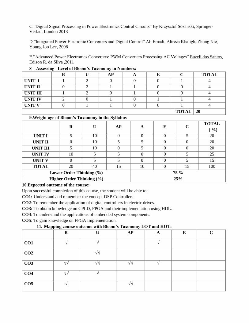
C.”Digital Signal Processing in Power Electronics Control Circuits” By Krzysztof Sozanski, Springer-
Verlad, London 2013
D.”Integrated Power Electronic Converters and Digital Control” Ali Emadi, Alireza Khaligh, Zhong Nie,
Young Joo Lee, 2008
E.”Advanced Power Electronics Converters: PWM Converters Processing AC Voltages” Euzeli dos Santos,
Edison R. da Silva ,2011
8 Assessing Level of Bloom’s Taxonomy in Numbers:
R U AP A E C TOTAL
UNIT I 1 2 0 0 0 1 4
UNIT II 0 2 1 1 0 0 4
UNIT III 1 2 0 1 0 0 4
UNIT IV 2 0 1 0 1 1 4
UNIT V 0 1 1 0 0 1 4
TOTAL 20
9.Weight age of Bloom’s Taxonomy in the Syllabus
R U AP A E C TOTAL
( %)
UNIT I 5 10 0 0 0 5 20
UNIT II 0 10 5 5 0 0 20
UNIT III 5 10 0 5 0 0 20
UNIT IV 10 5 5 0 0 5 25
UNIT V 0 5 5 0 0 5 15
TOTAL 20 40 15 10 0 15 100
Lower Order Thinking (%) 75 %
Higher Order Thinking (%) 25%
10.Expected outcome of the course:
Upon successful completion of this course, the student will be able to:
CO1: Understand and remember the concept DSP Controllers
CO2: To remember the application of digital controllers in electric drives.
CO3: To obtain knowledge on CPLD, FPGA and their implementation using HDL.
CO4: To understand the applications of embedded system components.
CO5: To gain knowledge on FPGA Implementation.
11. Mapping course outcome with Bloom’s Taxonomy LOT and HOT:
R U AP A E C
CO1 √ √ √
CO2 √√
CO3 √√ √√ √√ √
CO4 √√ √
CO5 √ √√

12. Mapping Course outcome with graduate attributes:
GA1 GA2 GA3 GA4 GA5 GA6 GA7 GA8 GA9 GA10 GA11 GA12
CO1 √√ √√ √ √√ √ √
CO2 √√ √√ √ √ √ √√ √ √ √
CO3 √√ √ √ √ √
CO4 √√ √ √√ √√
CO5 √ √ √
13. Mapping course outcome with programme outcomes:
PO1 PO2 PO3 PO4 PO5 PO6 PO7 PO8 PO9 PO10 PO11 PO12
CO1 √√ √√ √ √ √ √ √ √ √
CO2 √√ √√ √√ √ √√ √√ √ √
CO3 √√ √ √ √
CO4 √√ √ √√ √ √ √
CO5 √
14. Mapping with Programme Educational Objectives:
PEO1 PEO2 PEO3 PEO4 PEO5
CO1 √ √ √
CO2 √√ √√ √ √√
CO3 √√ √√ √√
CO4 √√ √√
CO5 √√ √ √
√√ Strongly agreed √ Moderately agreed

1. Course pre-requisites : Microprocessor and microcontroller.
2. Course learning objectives :
i. To familiarize the fundamental concepts of microprocessor architecture.
ii. To gain knowledge about high performance CISC architecture- PENTIUM.
iii. To gain knowledge about ARM microcontroller architecture.
iv. To study about MOTOROLA Microcontrollers viz. 68HC11.
v. To gain knowledge about PIC microcontroller
3. Expected Level of Output : Conceptual Level
4. Department Offered : Electrical and Electronics Engineering.
5. Nature of the Course : Group 7 – 75%Descriptive and 25% programming
Continuous Internal Assessment (CIA) : 40 Marks
Semester End Examination (SEE) : 60 Marks
6. Course Input :
Un
it N
o
Nam
e O
f T
he
Top
ic
Tex
t /
Ref
Book
s
Ch
ap
ter
No
Inst
ruct
ion
al
Hou
rs
Lev
el o
f B
loom
’s
Taxon
om
y
Course
Assessment
Factors
F1
F2
F3
F4
I
OVERVIEW
Generic Architecture--Instruction Set –
Data formats –Addressing modes –
Memory hierarchy – Register file
A 1,2,3 4 R
9
5 4 2
Cache – Virtual memory and paging –
Segmentation- pipelining
–The instruction pipeline – Pipeline
hazards – Instruction level parallelism –
Reduced
A 4,5 3 U 5 5 2
Instruction set –Computer principles –
RISC versus CISC. A 6 2 R 4 5 2
HIGH PERFORMANCE CISC ARCHITECTURE – PENTIUM
CPU Architecture- Bus Operations –
Pipelining – Brach predication – Floating
point unit
A,B 8,2 2 U 9
5 5 4
Operating Modes –Paging – Multitasking – A,B 8,5 2 U 5 4 5
Course Code Course Name Contact Hours
L T P C
17PE085 Advanced Microprocessors And Microcontrollers 3 0 0 3
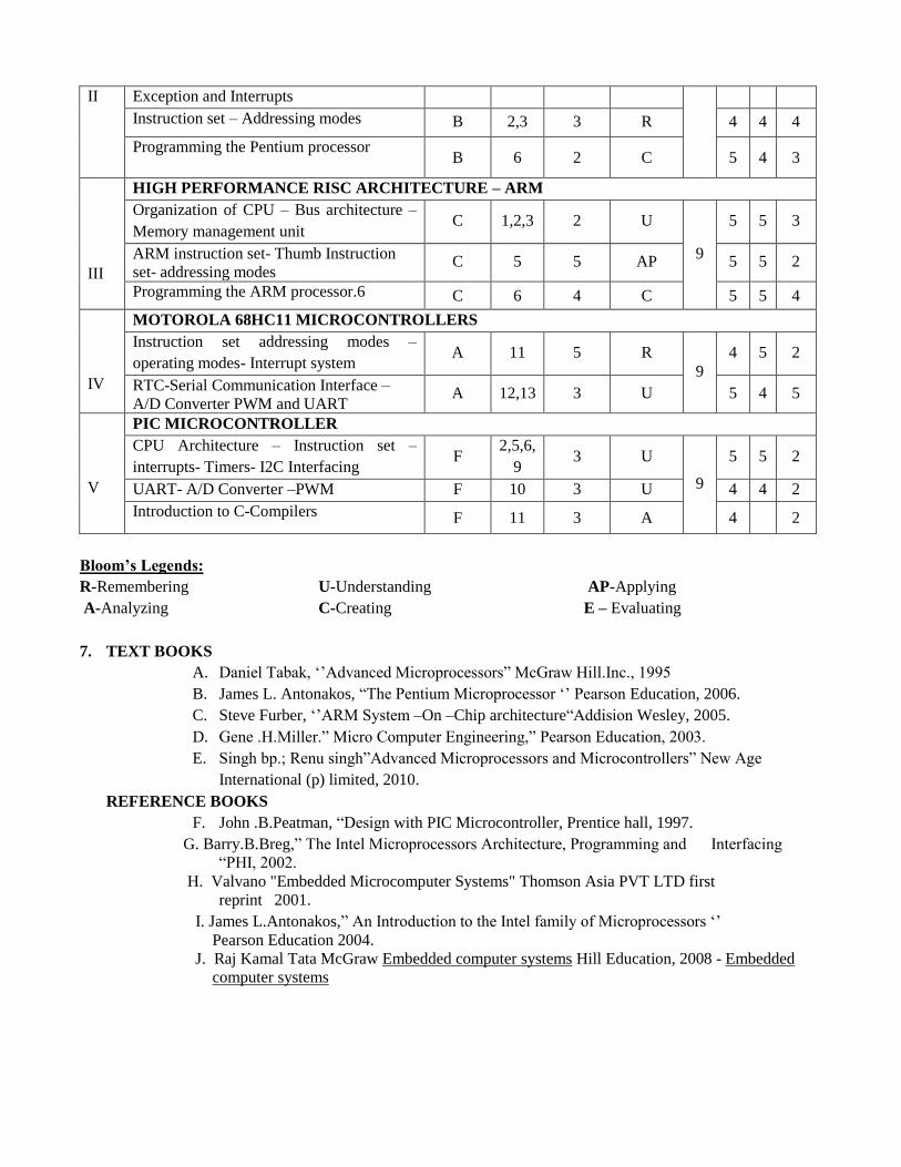
II Exception and Interrupts
Instruction set – Addressing modes B 2,3 3 R 4 4 4
Programming the Pentium processor
B 6 2 C 5 4 3
III
HIGH PERFORMANCE RISC ARCHITECTURE – ARM
Organization of CPU – Bus architecture –
Memory management unit C 1,2,3 2 U
9
5 5 3
ARM instruction set- Thumb Instruction
set- addressing modes C 5 5 AP 5 5 2
Programming the ARM processor.6 C 6 4 C 5 5 4
IV
MOTOROLA 68HC11 MICROCONTROLLERS
Instruction set addressing modes –
operating modes- Interrupt system A 11 5 R
9
4 5 2
RTC-Serial Communication Interface –
A/D Converter PWM and UART A 12,13 3 U 5 4 5
V
PIC MICROCONTROLLER
CPU Architecture – Instruction set –
interrupts- Timers- I2C Interfacing F
2,5,6,
9 3 U
9
5 5 2
UART- A/D Converter –PWM F 10 3 U 4 4 2
Introduction to C-Compilers F 11 3 A 4 2
Bloom’s Legends:
R-Remembering U-Understanding AP-Applying
A-Analyzing C-Creating E – Evaluating
7. TEXT BOOKS
A. Daniel Tabak, ‘’Advanced Microprocessors” McGraw Hill.Inc., 1995
B. James L. Antonakos, “The Pentium Microprocessor ‘’ Pearson Education, 2006.
C. Steve Furber, ‘’ARM System –On –Chip architecture“Addision Wesley, 2005.
D. Gene .H.Miller.” Micro Computer Engineering,” Pearson Education, 2003.
E. Singh bp.; Renu singh”Advanced Microprocessors and Microcontrollers” New Age
International (p) limited, 2010.
REFERENCE BOOKS
F. John .B.Peatman, “Design with PIC Microcontroller, Prentice hall, 1997.
G. Barry.B.Breg,” The Intel Microprocessors Architecture, Programming and Interfacing
“PHI, 2002.
H. Valvano "Embedded Microcomputer Systems" Thomson Asia PVT LTD first
reprint 2001.
I. James L.Antonakos,” An Introduction to the Intel family of Microprocessors ‘’
Pearson Education 2004.
J. Raj Kamal Tata McGraw Embedded computer systems Hill Education, 2008 - Embedded
computer systems

8. Assessing Level of Bloom’s Taxonomy in Numbers:
R U AP A E C TOTAL
UNIT I 2 1 1 0 0 0 3
UNIT II 1 2 1 0 0 1 4
UNIT III 0 1 0 1 0 1 3
UNIT IV 1 1 2 0 0 0 2
UNIT V 0 2 1 0 1 0 3
TOTAL 15
9. Weight age of Bloom’s Taxonomy in the Syllabus
R U AP A E C TOTAL
( %)
UNIT I 13.33 6.66 0 0 0 0 19.98%
UNIT II 6.66 13.33 0 0 0 6.66 26.65%
UNIT III 0 6.66 6.66 0 0 6.66 19.98%
UNIT IV 6.66 6.66 0 0 0 0 13.33%
UNIT V 0 13.33 0 6.66 0 0 19.98%
TOTAL 26.65 46.58 6.66 6.66 0 13.33 99.97%
Lower Order Thinking (%) 80 %
Higher Order Thinking (%) 20%
10. Expected outcome of the course:
Upon successful completion of this course, the student will be able to:
CO1: To familiarize the fundamental concepts of microprocessor architecture.
CO2: To gain knowledge about high performance CISC architectures.
CO3: To gain knowledge about high performance RISC architectures.
CO4: To study about MOTOROLA Microcontrollers viz. 68HC11
CO5: To study about PIC Microcontrollers.
11. Mapping course outcome with Bloom’s Taxonomy LOT and HOT:
R U AP A E C
CO1 √ √√
CO2 √ √√ √
CO3 √ √√ √
CO4 √ √√
CO5 √√ √
12. Mapping Course outcome with graduate attributes:
GA1 GA2 GA3 GA4 GA5 GA6 GA7 GA8 GA9 GA10 GA11 GA12
CO1 √√ √ √ √ √ √ √
CO2 √√ √ √√ √ √ √
CO3 √√ √ √ √ √ √
CO4 √√ √ √√ √√ √ √
CO5 √√ √ √ √ √ √

13. Mapping course outcome with programme outcomes:
PO1 PO2 PO3 PO4 PO5 PO6 PO7 PO8 PO9 PO10 PO11 PO12
CO1 √√ √√ √ √ √ √ √ √ √
CO2 √√ √√ √ √ √ √ √
CO3 √√ √√ √ √ √ √ √ √
CO4 √√ √√ √ √ √ √ √ √
CO5 √√ √√ √ √ √ √ √ √ √
14. Mapping with Programme Educational Objectives:
PEO1 PEO2 PEO3 PEO4 PEO5
CO1 √√ √√ √
CO2 √√ √√ √
CO3 √√ √√ √
CO4 √√ √√ √
CO5 √√ √√ √
√√ Strongly agreed √ Moderately agreed

![Vidya Digital Library - sudhinpk critical clearing angle for the condition described. (15 marks) (b) ... Derive an expression for Swingequation. (15 marks) {4 x 15 =60 marks]-"Vidya](https://img.pdfslide.us/doc/110x75/5ac011b37f8b9ae45b8bbc91/vidya-digital-library-sudhinpk-critical-clearing-angle-for-the-condition-described.jpg)