Magnetic Resonance in Medicine 52:979–993 (2004)

Published 2004 Wiley-Liss, Inc.

DOI 10.1002/mrm.20283 Published online in Wiley InterScience (www.interscience.wiley.com).

Received 24 November 2003; revised 5 April 2004; accepted 7 April 2004.2004 ISMRM Young Invesigator I.I. Rabi Finalist.

This article is a US Governmentwork and, as such, is in the public domain in the United States of America.

979

“Squashing Peanuts and Smashing Pumpkins”: How Noise Distorts Diffusion-Weighted MR Data

Derek K. Jones* and Peter J. Basser

Wiley-Liss, Inc.

*Correspondence to: Derek K. Jones, National Institutes of Health, Building 13, Room 3W16E, 13 South Drive, Bethesda, MD 20892-5772 USA. E-mail: jonesde@mail.nih.gov

Section on Tissue Biophysics and Biomimetics, Laboratory of Integrative Medicine and Biophysics, National Institute of Child Health and Human De­velopment, National Institutes of Health, Bethesda, Maryland, USA

ABSTRACT

New diffusion-weighted imaging (DWI) methods, including high-b, q-space, and high angular resolution MRI methods, attempt to extract information about non-Gaussian diffusion in tissue that is not provided by low-b-value (b = 1000 s mm-2) diffusion or diffusion tensor magnetic resonance imaging (DT­MRI). Additionally, DWI data with higher spatial resolution are being acquired to resolve fine anatomic structures, such as white matter fasciculi. Increasing diffusion-weighting or de­creasing voxel size can reduce the signal-to-noise ratio so that some DWI signals are close to the background noise level. Here we report several new artifacts that can be explained by con­sidering how background noise affects the peanut-shaped an­gular apparent diffusion coefficient (ADC) profile. These include an orientationally dependent deviation from Gaussian behavior of the ADC profile, an underestimation of indices of diffusion anisotropy, and a correlation between estimates of mean diffu­sivity and diffusion anisotropy. We also discuss how noise can cause increased gray/white matter DWI contrast at higher b values and an apparent elevation of diffusion anisotropy in acute ischemia. Importantly, all of these artifacts are negligible in the b-value range typically used in DT-MRI of brain (b = 1000 s mm-2). Finally, we demonstrate a strategy for ameliorat­ing the rectified noise artifact in data collected at higher b values. Magn Reson Med 52:979–993, 2004. Published 2004

†

Key words: diffusion-weighted; DWI; MRI; ADC; noise; artifacts; trace; FA; DT-MRI

INTRODUCTION

Sensitizing the MR signal to the diffusion of water mole­cules provides useful information about tissue character­istics in vivo (1), ranging from changes in acute ischemia (2) through characterization of anisotropic structures (e.g., 3,4) to reconstructions of white matter pathways through­out the brain (e.g., 5). Such information has been obtained mostly using diffusion-weighted (DW) image data with moderate resolution (e.g., 2.5 mm X 2.5 mm X 2.5 mm) and moderate diffusion weighting (b = 1000 s mm-2) sothat the diffusion displacement profile in each voxel can be adequately described by a Gaussian function (6). For example, the diffusion characteristics of a voxel contain­ing a single fiber population can be characterized by a tensor whose associated ellipsoid is prolate. In voxels containing multiple fiber populations (e.g., fibers cross-

ing), the diffusion characteristics observed at low b values can still be described by a single tensor, but the diffusion ellipsoid may be less prolate and may become spherical or even oblate (7). In such cases, the tensor model does not adequately reflect the underlying tissue microstructure, which can be problematic for applications such as tractog­raphy (5).

Several groups (7–17) have proposed methods for eluci­dating complex tissue microstructure by studying the non-Gaussian diffusion behavior that only becomes apparent at higher b values (6,8). For example, Frank’s spherical har­monic approach (9) collects DW data at b = 3000 s mm-2, whereas diffusion spectrum imaging (DSI) (11) (closely related to q-space imaging) (12) attempts to infer the dif­fusion displacement probability profile directly from dif­fusion-weighted data collected at very high b values (up to 20,000 of each DW image).

It is well known that noise in complex MR data are normally distributed, whereas the magnitude is Rician distributed (18,19). Consequently, in the absence of any true signal, the mean (T) and SD (uT) of the magnitude– reconstructed signal are given by the following:

T = u and uT=u 2- [1]2

,2

respectively, where u is the SD of the MR signal (18). Thus rectification of a noisy signal gives rise to a minimum signal measurable, which we refer to as the rectified noise floor. At low SNR, this has deleterious consequences for DWI data (20). The amplitude of the DW signal is overes­timated (due to the rectified noise floor), but the estimate of the non-DW signal (being far from the noise floor) is unaffected. Therefore the apparent diffusion coefficient (ADC) computed from the two signals will be underesti­mated (20). Another effect of noise relevant to DT-MRI is eigenvalue repulsion (21), which leads to the well-docu­mented overestimation of diffusion anisotropy at low SNR (e.g., 22).

Here we report several new artifacts of noise that are particularly relevant in DWI at high diffusion weightings or at low SNR. We show that under certain conditions, the diffusion anisotropy of the effective diffusion tensor, D, can be underestimated due to the presence of noise. We also show how artifactual correlations between diffusion-related parameters can be introduced by the presence of noise and how Gaussian diffusion characteristics can ap­pear non-Gaussian solely as a result of the rectified noise floor. Finally, we propose a strategy that serves to amelio­rate the problems associated with the rectified noise floor.

METHODS

Monte Carlo simulations were performed to investigate the effect of noise on diffusion-derived parameters. Diffu-

†

980 Jones and Basser

sion tensors were simulated with characteristics similar to those of brain white matter (i.e., constant trace (Tr(D) = 2.1 X 10-3 mm2 s-1) (6) but varying fractional anisotropy (FA) (23). Simulations were performed in two dimensions (2D) for graphical representations and three dimensions (3D) for quantitative studies. Appendix A shows how the diffusion tensors (for a given Trace and FA) and b matrices were defined for each case.

Investigating the Effect of the Noise Floor on the ADC Profile

For the noise-free diffusion tensors, the ADC was plotted as a function of angle with respect to the principal eigen­vector of the tensor (i.e., the eigenvector associated with the largest eigenvalue). In 2D, this is a simple polar plot; in 3D it is a plot in spherical coordinates. If the direction is given by the unit vector, g, then the ADC along that direc­tion, ADCg, is given by the projection of D along g as follows:

ADCg = gTDg. [2]

Next, the noise-free DW intensity along the direction, g, was computed as follows:

DWIg = I0 exp(-bADCg), [3]

where b is the scalar magnitude of the diffusion weighting, Io is the un-weighted signal (arbitrarily set to 1000 units), and DWIg is the diffusion-weighted intensity along g. Noise was then added in quadrature to both Io and DWIg. Noisy estimates of the ADC along the direction g, (ADCn

g ), were then computed using the following:

1 n nADCg = ln( I0 ), [4]

b DWIg n

where In o and DWIn

g are the noise-contaminated un­weighted and diffusion-weighted signals, respectively.1

1Note that this “two-point” approach (i.e., characterizing diffusion using data collected at two diffusion-weighting amplitudes, as opposed to using multiple diffusion-weighting amplitudes) is the approach most commonly adopted in the DWI community.

For each sampling orientation, 500 noisy estimates of ADCn

g were obtained, their mean, (ADCng ), computed, and

their distribution plotted.

Investigating the Effect of The Noise Floor on Diffusion Tensor Estimates

To characterize the effects of noise in DT-MRI experi­ments, two approaches were used. These are described in Appendix B.

Investigating the Effect of Sampling Scheme and Fitting Procedure

As stated in Footnote 1, in the literature the “two-point” approach (i.e., using DW data collected at just two b val­ues) is commonplace. However, collecting data at more b

values allows greater choice of strategies for estimating the ADC (i.e., linear fitting, weighted linear fitting, nonlinear fitting). The final part of this study therefore investigated the effect on the noisy ADC profile of (a) different sampling schemes and (b) different ADC estimation strategies. First, tensors with a given anisotropy and trace were chosen as described above (and in Appendix A). Next, for a given SNR2

2Note: For the remainder of the methods and results section, SNR is taken to mean the SNR of the b = 0 images.

a set of noisy DW intensities was computed for different numbers of equally spaced b values between the minimum (zero) and a maximum specified b value, bmax. We refer to the number of unique b values between zero and bmax inclusive as Nunique. Five different fitting proce­dures were employed as follows:

1. Two Point Method. This fitting approach was already described. Of the set of

DW intensities simulated at different b values, only the intensities simulated for zero diffusion weighting and the maximum diffusion weighting were used to estimate the ADC along each sampling orientation, using the model in Eq. [3].

2. Unweighted Linear Fit. All the simulated intensities collected at different b val­

ues were used to estimate the ADC from the model in Eq. [3], using linear regression but assuming that the SD asso­ciated with each log-transformed DW intensity was the same.

3. Weighted Linear Fit. This method also used linear regression, but differed

from Method 2 in that the SD of each log-transformed DW intensity, uln(DWI), was approximated by the following (24):

uln(DWI) = u/DWI, [5]

where u is the SD of the (non-log-transformed) diffusion-weighted intensity, DWI. In the linear regression, each observation was weighted by the SD, uln(DWI).

4. Nonlinear Fit. This method involved fitting all the simulated DWIs to

the model in Eq. [3] using Levenberg–Marquardt nonlinear regression.

5. Nonlinear Fit with Noise Estimation. In this method a noise parameter was estimated as part

of the fitting procedure. The noisy diffusion-weighted in­tensity was modeled according to the following:

1

DWIN = (DWI2NF

2)2

where DWIN and DWINF are the noisy and noise-free dif­fusion-weighted intensities respectively and is the noise-parameter to be estimated. Again, Levenberg–Marquardt nonlinear regression was used for the fitting procedure.

Estimating the noise parameter introduces an extra de­gree of freedom, which necessitates the collection of more data to achieve the same reliability as a model with fewer parameters. Furthermore, the robustness of this last fitting

981 “Squashed Peanuts” in Diffusion-Weighted Imaging

procedure is likely to be increased if the data contain multiple points at which the signal is predominantly noise. Such data could be obtained in practice on an MR scanner by employing extremely high b values (e.g., b : 40,000 s mm-2). However, there are two problems associ­ated with this approach. First, if there is true restricted (as opposed to hindered) diffusion, then the noise-free DW signal at high b values may be nonzero. Second, acquiring many samples at high b values unacceptably increases the acquisition time. An alternative approach is to obtain mul­tiple measurements of the signal outside of the brain (i.e., in the background and in regions where there are no phase-encode artifacts) and then assign these values to be the diffusion-weighted intensities at the high b values. This approach provides a large number of estimates of the signal obtained at extremely high b values without increas­ing scanning time. We refer to these measurements as “extreme b-value measurements.” To reproduce this ap­proach in the Monte Carlo simulations, we simply ob­

tained Nextreme estimates of the rectified signal in the ab­sence of any true signal and equated these measurements with those obtained at a series of Nextreme equally spaced b values between 40,000 s mm-2 and 10,000 s mm-2. To quantify the efficacy of this last approach, the mean dif­ference between the noise-free ADC profile and the ADC profile obtained using this last fitting approach was com­puted. A number of ADC profiles were then obtained using the five different estimation procedures for data simulated with different numbers of unique b values, (Nunique), and different numbers of extreme b value measurements, (Nextreme).

RESULTS

The effect of the rectified noise floor on the diffusion-weighted signal attenuation is shown in Fig. 1, where results are shown for two diffusivities: 0.1 X 10-3 mm2 s-1

and 1.0 X 10-3 mm2 s-1. These values are representative of

FIG. 1. Plots of the diffusion-weighted intensity and log of the diffusion-weighted intensity as a function of b value, for two differ­ent diffusivities: 0.1 X 10-3 mm2

s-1 (a and b) and 1.0 X 10-3 mm2

s-1 (c and d). The signal-to-noise ratio (in the b = 0 image) was 15:1. The dotted line corresponds to the log of the rectified noise floor, computed using Eq. [2]. The upper and lower traces show the signal in the presence and ab­sence of noise, respectively. The error bars correspond to 1.96 u, where u is the SD of the diffusion-weighted signal intensity at a par­ticular b value, therefore repre­senting the 95% confidence inter­val. The dotted line represents the mean of the noise measured in the absence of any true signal (Eq. [2]) and the dotted error bars show the 95% confidence interval (computed using Eq. [3]. Note that in a and b, the two traces are superimposed. The asterisk in Fig. 1D shows the point at which the Eq. [11] is satisfied. Figures 1e and 1f show the same data ana­lyzed as a q-space experiment. In this case q is taken as the square root of the b value (which will be directly proportional to the true value of q if the diffusion-time, L, remains fixed; see Appendix C). The dotted line corresponds to the value of E(q) resulting from the rectified noise floor. In Fig. 1e, the E(q) plots from the noise-free and noisy data are superimposed.

982 Jones and Basser

the largest and smallest eigenvalues of a diffusion tensor with Trace = 2.1 X 10-3 mm2 s-1 (4) and FA = 0.9. In Fig. 1A, the ADC is sufficiently low that the DW intensity never reaches the noise floor. Consequently, over the b-value range shown, the plot of log-transformed intensity versus b (Fig. 1B) has a constant slope, indicating that the estimated diffusivity is independent of b and will therefore be deter­mined accurately. Conversely, in Fig. 1C, the DW intensity begins to approach the noise floor within the range of b = 1000 s mm-2 to 2000 s mm-2. In this range, the slope of the log-transformed intensity versus b becomes nonlinear (Fig. 1D) and as b is increased further, the DW intensity agrees well with the theoretical value of the noise floor (dotted line) predicted by Eq. [1].

By setting the diffusion-weighted intensity in Eq. [4] to the mean background signal, T, we can obtain an order of magnitude estimate for ADCmax, the maximum expected value of the diffusivity that can be measured without suc­cumbing to the squashed peanut effect, for a given b value, unweighted signal, and level of background noise, that is,

1 ADCmax = ln( I0). [7]

b T

The asterisk in Fig. 1D shows the point at which Eq. (7) is satisfied. Note, however, that T only represents the mean of the rectified noise signal and, as shown by the error bars in Figs. 1A and 1C, the noise floor influences the estima­tion of the ADC even when the DW signal is significantly greater than T. Figures 1E and 1F show the same data analyzed as a “q-space” experiment (12), where E(q) is

plotted versus “q” and where we have taken “q” to be proportional to the square root of b (see Appendix C).

Figure 2 shows the noise-free and noisy ADC profiles obtained for a 2D tensor with FA = 0.90, Trace = 2.1 X 10-3 mm2 s-1, and SNR = 15:1 (where the SNR is the signal-to-noise ratio in the image obtained with no diffu­sion weighting). As others have shown (7,8,25,26), the mean ADC profile assumes the shape of a peanut when the diffusion ellipsoid is prolate. The diffusivities along the major and minor axes of the peanut are equal to the major and minor eigenvalues ( 1 and 2) of D. The analytical form for this ADC profile is given by the following (26):

D0 = 1cos2 0 + 2sin2 0, [8]

where D0 is the diffusivity along the projection at angle 0 to the major eigenvector of the diffusion tensor. Note that the noisy ADC profile deviates from the theoretical (noise-free) profile, with the former appearing “squashed” along its long axis. This deviation is attributable to the underesti­mation of the higher diffusivities observed along that axis. The data in Fig. 1 correspond to the diffusivities observed along the major and minor axes of the peanut presented in Fig. 2. Clearly, along the minor axis, the effect of the noise floor is insignificant and so the profile of the peanut is unaffected along that axis. At some polar angle to the long axis of the peanut, 0B, the profile begins to deviate signif­icantly from that predicted by Eq. [7]. Again, it is possible to obtain an order of magnitude estimate of this breakpoint by combining Eqs. [7] and [8], that is:

FIG. 2. a shows the ADC profile obtained for a 2D tensor with mean diffusivity = 0.7 X 10-3 mm2 s-1 and fractional anisotropy = 0.9. The signal-to-noise ratio was set to 15:1 and the b value set to 2500 s mm-2. The dotted line corresponds to the noise-free ADC profile predicted by Eq. [12], whereas the solid line corresponds to the mean of the noisy estimates of ADC at each projection, 0, to the major axis of the peanut. The diffusivities along the major and minor axes of the peanut correspond to the major and minor eigenvalues of the diffusion tensor. The asterisks mark the predicted points at which the noisy profile should deviate from the noise-free profile. b and c show the distribution of the ADCs measured at 0 = 90° and 0° respectively. Note that the histograms are plotted with different scales to allow the detail of the plots to be fully appreciated.

983 “Squashed Peanuts” in Diffusion-Weighted Imaging

12 01cos B + 2sin2 0B = ln(I0),

b T[9]

which is readily solved for 0B:

1 - ln(I0)b T0B = sin-1 , [10] 1

( 1 - 2)

in which 1 > 2. The asterisks on Fig. 2 correspond to the “breakpoint” angles, 0B, computed from Eq. [10]. The as­terisks do not correspond exactly to the points where the noisy and noise-free ADC profiles appear to deviate from each other. This is to be expected, as Eq. [10] is a liberal measure that assumes that only the mean noise floor af­fects the estimate of the ADC.

A statistical framework is useful for understanding the cause of the squashed peanut. Figures 2B and 2C show the distribution of ADC measurements at two sampling angles, 0 = 90° and 0 = 0°, respectively. Figure 2B appears to be Gaussian, whereas Fig. 2C appears skewed and non-Gaus­sian. The ADC distributions were compared with Gaussian

distributions using the Kolmogorov–Smirnoff function test in MATLAB (The Mathworks, Natick, MA) using an a value of 0.001. The distribution of ADC values sampled across the neck of the peanut (0 = 90°) was found to be Gaussian, but the distribution at 0 = 0° was non-Gaussian. The crosses in Fig. 2 indicate the points on the ADC profile at which the transition from Gaussianity to non-Gaussian­ity occurred, as determined by the Kolmogorov–Smirnoff test. As the Kolmogorov-Smirnoff test considers the entire distribution of ADC values, rather than just the mean (as in Eq. [10]), this measure will be a more sensitive indicator of peanut squashing than Eq. [10].

Figure 3 shows the noisy ADC profiles for six tensors with FA ranging from 0 to 1 and for b values ranging from 1000 s mm-2 to 10,000 s mm-2. In general, as the b value is increased, the peanuts are increasingly squashed along the long axis. However, as predicted from Fig. 1 (i.e., low diffusivities are not affected by the noise floor, while high diffusivities are), below a certain SNR threshold and for a given Trace, the relative signal loss (and therefore squash­ing of the peanut) depends on the anisotropy. Further­more, the amount of squashing also varies according to the

FIG. 3. ADC profiles for tensors with fractional anisotropy ranging from 0 to 1 and mean diffusivity = 0.7 X 10-3 mm2 s-1. Ten ADC profiles are shown for each tensor, corresponding to b = 1,000; 2,000; 3,000; 4,000; 5,000; 6,000; 7,000; 8,000; 9,000; and 10,000 s mm-2. The outermost profile corresponds to b = 1000 s mm-2, whereas the innermost corresponds to b = 10,000 s mm-2.

984 Jones and Basser

orientation. For example, for FA = 0, the reduction in the measured ADC is the same in all directions and so the anisotropy (i.e., zero) remains the same for all b values. Nevertheless, the mean ADC is reduced by the presence of noise. Assuming a constant Trace, as D becomes increas­ingly anisotropic, the diffusivity along the long axis of the peanut increases while in the orthogonal direction it de­creases. Consequently, the ADC profile becomes more squashed along the long axis of the peanut and less squashed along the orthogonal axis. A result of this differ­ential quashing is that the ADC profile becomes increas­ingly circular (less peanut-shaped) as the b value is in­creased, therefore leading to an underestimation of anisot­ropy.

The effect of the rectified noise floor on the relationship between measured FA and SNR is shown in Fig. 4 for four different b values. In the low b domain (b = 1000 s mm-2), the familiar pattern of overestimation of the anisotropy at low SNR and convergence to the true anisotropy at high SNR (22) is observed. At b = 3000 s mm-2, the estimates of FA appear to be relatively unbiased and insensitive to the SNR. However, as the b value is increased further, the anisotropy becomes underestimated.

FIG. 4. Relationship between estimated fractional anisotropy and signal-to-noise ratio for a simulated diffusion tensor whose true fractional anisotropy is 0.7 (represented by the horizontal dotted line) for four different b values: (a) 1000 s mm-2; (b) 3000 s mm-2; (c) 5000 s mm-2; and (d) 7000 s mm-2. The circles show the mean of 10,000 estimates, whereas the error bars show the SD.

Another way to investigate the influence of noise on FA and Trace measurements is to keep the SNR fixed (in the b = 0 image) and vary the b value. Typical results obtained from this type of simulation are presented in Fig. 5, in which the FA of the tensor has been estimated for b values in the range of 50 s mm-2 to 10,000 s mm-2. The degree of

squashing of the peanut, for a given SNR and b value, depends on the FA as seen in Fig. 3. Further, as FA in­creases, the deviation of the noisy profile from the ideal­ized peanut is reduced across its neck (i.e., in the direction perpendicular to the long axis). Because the Trace is equal to the sum of the diffusivities in the orthogonal directions, it is reasonable to expect that the Trace will be progres­sively underestimated as anisotropy increases which is confirmed in Fig. 6. For example, at b = 2500 s mm-2, there is approximately a 10% difference in the estimated Trace for a tensor with zero FA and a tensor with FA close to unity. This effect becomes more pronounced as the b-factor is increased.

Figure 7 shows the estimated FA as a function of true FA (i.e., anisotropy in the absence of noise) for the same range of b values. Note that at all b values greater than approxi­mately 1500 s mm-2, the true anisotropy is underesti­mated—and the underestimation becomes progressively worse at higher b values. However, the shapes of the curves also change at higher b values such that the low anisotropies become progressively more underestimated compared to higher anisotropies as the b factor is in­creased.

The effect of reducing the Trace on the estimated FA is shown in Fig. 8 for a diffusion tensor with an initial mean diffusivity of 0.7 X 10-3 mm2 s-1 and a (noise-free) FA of 0.75 [values which are representative of deep white matter (4)]. At b = 1000 s mm-2, there appears to be little corre­lation between Trace and estimated FA. However, as the b

985 “Squashed Peanuts” in Diffusion-Weighted Imaging

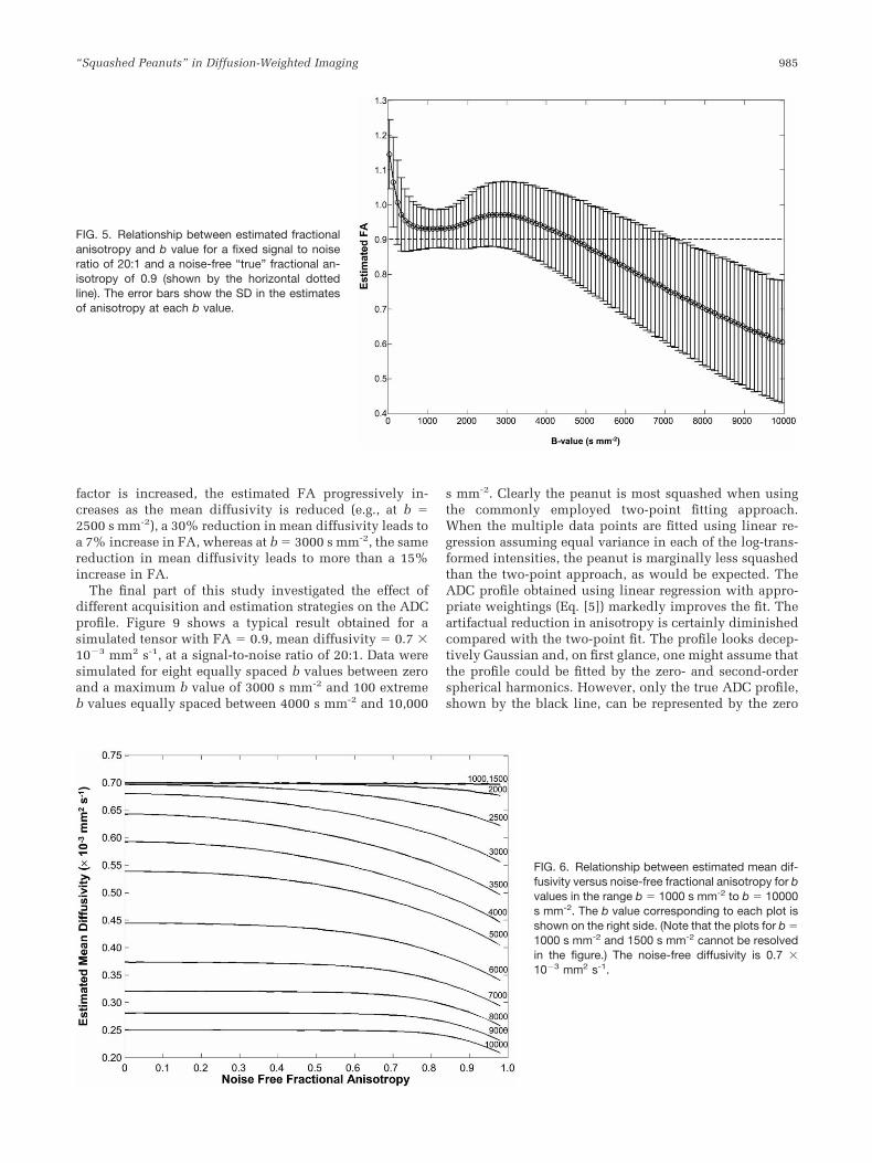
FIG. 5. Relationship between estimated fractional anisotropy and b value for a fixed signal to noise ratio of 20:1 and a noise-free “true” fractional an­isotropy of 0.9 (shown by the horizontal dotted line). The error bars show the SD in the estimates of anisotropy at each b value.

FIG. 6. Relationship between estimated mean dif­fusivity versus noise-free fractional anisotropy for b values in the range b = 1000 s mm-2 to b = 10000 s mm-2. The b value corresponding to each plot is shown on the right side. (Note that the plots for b =1000 s mm-2 and 1500 s mm-2 cannot be resolved in the figure.) The noise-free diffusivity is 0.7 X 10-3 mm2 s-1.

factor is increased, the estimated FA progressively in­creases as the mean diffusivity is reduced (e.g., at b = 2500 s mm-2), a 30% reduction in mean diffusivity leads to a 7% increase in FA, whereas at b = 3000 s mm-2, the same reduction in mean diffusivity leads to more than a 15% increase in FA.

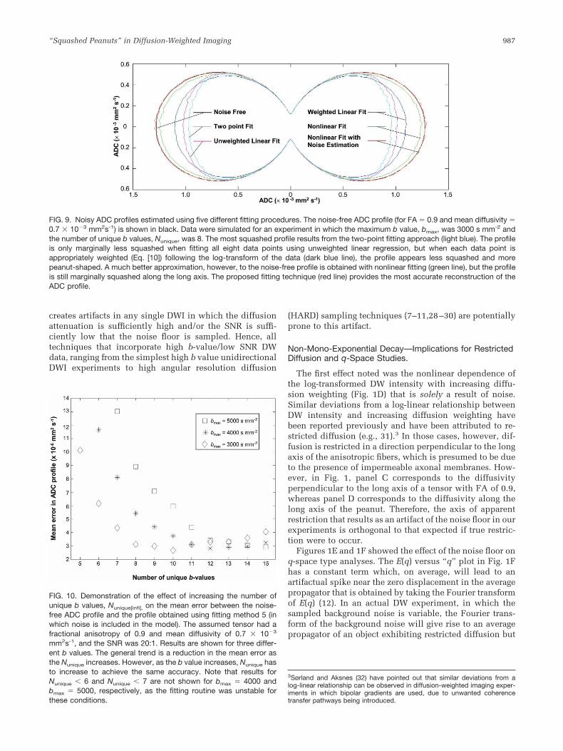
The final part of this study investigated the effect of different acquisition and estimation strategies on the ADC profile. Figure 9 shows a typical result obtained for a simulated tensor with FA = 0.9, mean diffusivity = 0.7 X 10-3 mm2 s-1, at a signal-to-noise ratio of 20:1. Data were simulated for eight equally spaced b values between zero and a maximum b value of 3000 s mm-2 and 100 extreme b values equally spaced between 4000 s mm-2 and 10,000

s mm-2. Clearly the peanut is most squashed when using the commonly employed two-point fitting approach. When the multiple data points are fitted using linear re­gression assuming equal variance in each of the log-trans­formed intensities, the peanut is marginally less squashed than the two-point approach, as would be expected. The ADC profile obtained using linear regression with appro­priate weightings (Eq. [5]) markedly improves the fit. The artifactual reduction in anisotropy is certainly diminished compared with the two-point fit. The profile looks decep­tively Gaussian and, on first glance, one might assume that the profile could be fitted by the zero- and second-order spherical harmonics. However, only the true ADC profile, shown by the black line, can be represented by the zero

986 Jones and Basser

FiG. 7. Relationship between estimated fractional anisotropy versus “true” (noise-free) fractional an­isotropy for b values in the range b = 1000 s mm-2

to b = 10000s mm-2. The b value corresponding to each plot is shown on the right side. (Note that the plots for b = 1000 s mm-2, 1500 s mm-2, and 2000 s mm-2 cannot be resolved in the figure.) The noise-free mean diffusivity is constant and equal to 0.7 X 10-3 mm2 s-1.

FIG. 8. The effect of reducing the mean diffusivity on the estimated anisotropy of a diffusion tensor with mean diffusivity of 0.7 X 10-3 mm2s-1 and fractional anisotropy of 0.75. The graph shows the changes in mean diffusivity and anisotropy as per­centage changes, for four different b values: 1000 s mm-2, 2000 s mm-2, 2500 s mm-2, and 3000 s mm-2.

and second-order harmonics. The profile obtained using nonlinear fitting provides a good approximation to the noise-free profile, but, nevertheless, is still noticeably squashed along the long axis of the peanut which, once again, means that higher-order spherical harmonics would be needed to fully describe it. Finally, the result obtained using the proposed fitting method in which a noise param­eter is included in the fitting procedure provides the most accurate reconstruction of the noise-free ADC profile.

With simulated data for which bmax = 3000 s mm-2, SNR = 20:1, FA = 0.9, and mean diffusivity = 0.7 X 10-3

mm2 s –1, increasing Nunique reduced the overall deviation between the noise-free ADC profile and the fitted ADC profile (see Fig. 10). Moreover, as bmax is increased, Nunique

must be increased to achieve the same level of accuracy (see Fig. 10). The fitting procedure was unstable for Nunique

< 5, by which we mean that at least one of the projected ADCs was overestimated by an order of magnitude or greater. As the b value was increased, the minimum value of unique b values needed for a stable estimate of the ADC profile also increased. For example, for values of bmax of 3000 s mm-2, 4000 s mm-2, and 5000 s mm-2, the minimum number of unique b values was 5, 6, and 7 respectively.

DISCUSSION

We have seen various ways in which noise affects mea­surements in DWI experiments. The rectified noise floor

987 “Squashed Peanuts” in Diffusion-Weighted Imaging

FIG. 9. Noisy ADC profiles estimated using five different fitting procedures. The noise-free ADC profile (for FA = 0.9 and mean diffusivity = 0.7 X 10-3 mm2s-1) is shown in black. Data were simulated for an experiment in which the maximum b value, bmax, was 3000 s mm-2 and the number of unique b values, Nunique, was 8. The most squashed profile results from the two-point fitting approach (light blue). The profile is only marginally less squashed when fitting all eight data points using unweighted linear regression, but when each data point is appropriately weighted (Eq. [10]) following the log-transform of the data (dark blue line), the profile appears less squashed and more peanut-shaped. A much better approximation, however, to the noise-free profile is obtained with nonlinear fitting (green line), but the profile is still marginally squashed along the long axis. The proposed fitting technique (red line) provides the most accurate reconstruction of the ADC profile.

FIG. 10. Demonstration of the effect of increasing the number of unique b values, Nunique[infi], on the mean error between the noise-free ADC profile and the profile obtained using fitting method 5 (in which noise is included in the model). The assumed tensor had a fractional anisotropy of 0.9 and mean diffusivity of 0.7 X 10-3

mm2s-1, and the SNR was 20:1. Results are shown for three differ­ent b values. The general trend is a reduction in the mean error as the Nunique increases. However, as the b value increases, Nunique has to increase to achieve the same accuracy. Note that results for Nunique < 6 and Nunique < 7 are not shown for bmax = 4000 and bmax = 5000, respectively, as the fitting routine was unstable for these conditions.

creates artifacts in any single DWI in which the diffusion attenuation is sufficiently high and/or the SNR is suffi­ciently low that the noise floor is sampled. Hence, all techniques that incorporate high b-value/low SNR DW data, ranging from the simplest high b value unidirectional DWI experiments to high angular resolution diffusion

(HARD) sampling techniques (7–11,28–30) are potentially prone to this artifact.

Non-Mono-Exponential Decay—Implications for Restricted Diffusion and q-Space Studies.

The first effect noted was the nonlinear dependence of the log-transformed DW intensity with increasing diffu­sion weighting (Fig. 1D) that is solely a result of noise. Similar deviations from a log-linear relationship between DW intensity and increasing diffusion weighting have been reported previously and have been attributed to re­stricted diffusion (e.g., 31).3

3Sørland and Aksnes (32) have pointed out that similar deviations from a log-linear relationship can be observed in diffusion-weighted imaging exper­iments in which bipolar gradients are used, due to unwanted coherence transfer pathways being introduced.

In those cases, however, dif­fusion is restricted in a direction perpendicular to the long axis of the anisotropic fibers, which is presumed to be due to the presence of impermeable axonal membranes. How­ever, in Fig. 1, panel C corresponds to the diffusivity perpendicular to the long axis of a tensor with FA of 0.9, whereas panel D corresponds to the diffusivity along the long axis of the peanut. Therefore, the axis of apparent restriction that results as an artifact of the noise floor in our experiments is orthogonal to that expected if true restric­tion were to occur.

Figures 1E and 1F showed the effect of the noise floor on q-space type analyses. The E(q) versus “q” plot in Fig. 1F has a constant term which, on average, will lead to an artifactual spike near the zero displacement in the average propagator that is obtained by taking the Fourier transform of E(q) (12). In an actual DW experiment, in which the sampled background noise is variable, the Fourier trans­form of the background noise will give rise to an average propagator of an object exhibiting restricted diffusion but

988 Jones and Basser

having a complex multilobular structure, similar to those observed in Diffusion Spectrum Imaging (DSI) (11) studies of gray matter in brain tissue.

Implications for Spherical Harmonic Fitting Approaches

Pajevic and Basser (27) recently demonstrated that for (SNR > 5) and for b values used in typical neurologic DT-MRI experiments (b = 1000 s mm-2), the distribution of diffusion tensor elements in DT-MRI experiments was multivariate Gaussian. Because the ADC is a projection of the tensor along a specific direction (see Eq. [2]), it is expected that the probability distribution of ADCs in all directions would also be Gaussian. However, surprisingly, at higher b values, we found significant deviations from the Gaussian model using the Kolmogorov–Smirnoff test. We showed that the distribution of individual ADC mea­surements about the mean is Gaussian only up to a certain point along the neck of the peanut, but at some angle 0B to the long axis, it becomes non-Gaussian. At this transition point, the observed profile begins to deviate from the the­oretical noise-free (i.e., peanut-shaped) profile.

Frank (9) showed that the orientational ADC profile for single fiber populations can be adequately described by the zero- and second-order spherical harmonics. However, to describe the ADC profile arising from multiple fiber populations, higher-order spherical harmonics must be invoked, which is taken to indicate increasing tissue com­plexity (10). However, in this study we have seen that even for a single fiber population, which is perfectly described by a single tensor in the absence of noise, the effect of the rectified noise floor is to squash the ends of the ADC profile causing it to deviate from the peanut-shape ex­pected in a single fiber. (We note that in Fig. 2 of Hirsch et al. (30), although not commented upon, there is also evi­dence of squashing of the peanut along the long axis, but not the short axis.) In such cases, the profile will not be adequately described by only the zero- and second-order spherical harmonics—higher-order harmonics are re­quired.

Without attending to the sources of deviation from the Gaussian peanut profile, (which also include other sources such as misregistration of DW images, uncorrected pulsa­tility artifacts, and eddy-current distortions in addition to the noise effect reported here), one could erroneously as­cribe more structural complexity to tissue than physically exists. The effect of increasing b value on the squashing of the peanut is clearly seen in Fig. 3. At b = 1000 s mm-2

(which is typical of the b values used in most DT-MRI experiments), the shape of the ADC profiles agree well with the noise-free profile for all levels of anisotropy, and (although we have not verified it experimentally) it is expected that the ADC profile could be adequately de­scribed by the zero- and second-order spherical harmonic. However, as the b value is increased further, the ADC profile begins to deviate significantly from the noise-free profile, with this effect being most marked in the more anisotropic media. This should be a major concern for those approaches that utilize b values greater than, say, 1500 s mm-2 and analyze the angular profile of either the ADC or the DW intensity. One may naively think that the solution might be to employ the high-angular resolution

sampling techniques with relatively low b values. How­ever, in the low b-value domain, diffusion in tissue can always be adequately characterized by a single effective diffusion tensor (6), necessitating the use of larger b values to detect non-Gaussian diffusion. Indeed, Frank (7) showed that at low b values, the ADC profile for two orthogonal fibers could be adequately characterized by a single oblate tensor, but this was not the case at b = 3000 s mm-2. Hence, for the approaches that aim to extract more information than that provided by a single diffusion tensor model, the problem of the rectified noise floor is inescap­able. However, to the best of our knowledge, its effect has, so far, not been accounted for.

A New Effect of Noise on Anisotropy Measurements

In 1996, Pierpaoli and Basser reported the effect of noise on different measures of diffusion anisotropy (22). One of their findings was that the degree of anisotropy becomes progressively overestimated (i.e., the estimates are biased) as the SNR decreases. These experiments were performed with b < 1000 s mm-2 and, in this range, our results (see Fig. 4A) duplicate their findings. However, the results also show that had Pierpaoli and Basser considered experi­ments with higher b values, they might have concluded that noise has a different effect on anisotropy measures. Indeed, if their experiments had been performed with b = 3000 s mm-2, they might have concluded that FA values were relatively unbiased (see Fig. 4B). As the b factor is increased further (i.e., b > 3000 s mm-2), the anisotropy becomes underestimated for all levels of SNR greater than approximately 7:1.

Two competing mechanisms can explain the depen­dence of FA on SNR seen in Fig. 4. The first is eigenvalue repulsion (21) for moderate b values (by which we mean the range of b values in which the DW intensity does not approach the rectified noise floor); the second is squashing of the peanut, which begins to dominate as the b value is increased (and/or SNR is decreased). These competing mechanisms are evident in Fig. 5, which shows the esti­mated FA as a function of b value. There are three distinct regions in the plot. First, in the range of b = 1000 s mm-2, the SNR of the DW images will be high. However, the most biased estimates of anisotropy (i.e., overestimated anisot­ropy) are found in this domain. This is probably attribut­able to the diffusion weighting being insufficient to obtain a good estimate of the diffusivity along each sampling orientation. (It has been shown that the optimal diffusion weighting for diffusivity measurements is b = 1.11 / ADC (33).4

4Although it should be noted that this calculation was performed neglecting the associated T2 decay associated with diffusion-weighted spin-echo exper­iments. By including transverse relaxation in the optimization of diffusion-weighted sequences, Jones et al. (34) have shown that the optimal b factor is approximately 30% less than this in a typical diffusion-weighted MRI exper­iment.

The second phase in the plot (b = 1100 s mm-2 to b = 3000 s mm-2) shows a gradual rise in the estimated FA, which is most likely attributable to eigenvalue repulsion effects (21). As the b value is increased, the SNR of the DW image will decrease and, as Pierpaoli and Basser (22) showed, this leads to increasing overestimation of the

989 “Squashed Peanuts” in Diffusion-Weighted Imaging

anisotropy. The third phase of the plot shows a gradual decline in the estimated anisotropy. During this phase, the squashed peanut mechanism dominates. Frank (7) pro­posed an anisotropy measure based on the variance of a set of ADC measurements obtained along a large number of directions. The key idea was that in regions where fibers cross, for example, while measures such as FA and relative anisotropy (23) would be low, the variance of the ADC measurements would be large. Although this overcomes this problem in principle, the variance of the ADC mea­surements as a measure of anisotropy is also susceptible to the squashed peanut artifact, that is, as the peanut be­comes increasingly squashed, the ADC profile becomes increasingly spherical and hence reducing its variance and the computed anisotropy.

Artifactual Correlations between Trace and Anisotropy

The effect of the noise floor is to introduce an artifactual correlation between mean diffusivity and anisotropy (see Fig. 6). If not accounted for, this can bias results of exper­imental studies that assume independence of Trace and FA. Just how important this artifactual correlation is when performing independent statistical tests of anisotropy and mean diffusivity data obtained from the same voxel is worthy of further investigation. We have also shown that the estimated Trace in tissue is dependent on the SNR and the b value used. Although the noise sensitivity of anisot­ropy measurements has been previously documented, to date, the Trace has been assumed to be relatively noise-insensitive (22). Our results suggest that it would be good practice (for direct comparisons of Trace values obtained from studies performed at different b values, image reso­lutions, and SNRs) for authors to include the SNR of their experiments when reporting their findings.

Artifactual Increase in Gray Matter/White Matter Contrast and Underestimation of Anisotropy at Higher b Values

A further consequence of the relationship between Trace and FA shown in Fig. 6 is that, for a given brain, the contrast between gray and white matter in DWI or in mean diffusivity maps will increase as the b factor increases. In mean diffusivity maps, white matter would appear in­creasingly hypointense compared to gray matter as the b factor is increased. This effect arises because white matter has higher anisotropy than gray matter and hence experi­ences more “squashing of the peanut” as the b factor is increased. De Lano et al. (13) and Yoshiura et al. (15) have reported this trend between increased b factors and in­creased white matter/gray matter contrast. However, they suggested multiexponential diffusion behavior as the un­derlying mechanism causing this phenomenon. We are not suggesting that the squashed peanut phenomenon alone produced the patterns noted by these groups, but it may have contributed to the gray matter/white matter contrast they observed. We suggest, however, that this new mech­anism be considered in future studies before conclusions regarding multiexponential diffusion are drawn.

Apparent Elevation of Anisotropy in Acute Ischemia

Undoubtedly the most useful application of DWI to date has been in the study of acute ischemia (e.g., 2). Within the

first few hours after the onset of ischemia, there is a de­crease in the mean diffusivity of the ischemic tissue of approximately 30%. It is not difficult to envisage that this reduction in mean diffusivity will tend to increase the apparent anisotropy in a high b-value/low SNR experi­ment. If, prior to the ischemic reduction in diffusivity, the rectified noise floor is sampled, then the true anisotropy will be underestimated (see Fig. 3). During the ischemia, the 30% reduction in diffusivity will result in less squash­ing of the peanut along its long axis—and hence there will be an apparent increase in the anisotropy of the tensor. This is confirmed in Fig. 8, which shows the effect exac­erbated at higher b values. At b = 1000 s mm-2, the anisot­ropy remains approximately constant as the diffusivity is reduced. Note, however, that at b = 3000 s mm-2, a reduc­tion of 30% in mean diffusivity gives rise to a 15% in­crease in the estimated anisotropy.

Several groups (e.g., 35,36) have reported elevated an­isotropy in acute ischemia. Maier et al. (35) first suggested that the elevated anisotropy might be explained by the swelling of fibers causing further restriction of extracellu­lar fluid in the direction perpendicular to the long axis of the fiber. Sotak (37) in a recent review of the uses of diffusion imaging in stroke also raised the possibility that the elevation might somehow be related to cessation of motion/flow or perhaps to the effect of SNR reported else­where (22). [In the latter case, however, a reduced diffu­sivity would lead to reduced signal attenuation in the DWI and consequently higher SNR which, from the findings of Pierpaoli and Basser (22), would lead to a reduction in the estimated anisotropy]. In short, in acute ischemia studies where the SNR is low, or the b value has been increased (which is often done to increase the conspicuity of acute ischemic lesions), elevated anisotropies should be inter­preted extremely carefully.

Potential Remedies

Finally, having discussed all the artifacts introduced by the squashed peanut phenomenon, what are the remedies? One solution is, of course, to ensure that the SNR is suffi­ciently high (even using the highest b values) and/or the maximum b value sufficiently low, such that the rectified noise floor is never sampled. SNR can be boosted, for example, by using higher magnetic field strengths, surface coils, and stronger gradients (resulting in shorter echo times and therefore higher SNR per unit time for a given b value). However, such approaches can be costly and/or impractical. For a fixed SNR, it is therefore necessary to ensure that the b value is sufficiently low to ensure that the artifact does not manifest itself. In Appendix D, we show how to compute an order of magnitude estimate of the maximum b value that should be used for a given SNR, Trace and FA. For brain parenchyma, assuming a Trace of 2.1 X 10-3 mm2 s-1 (4), a typical SNR of 20:1 and account­ing for all possible anisotropies (ranging from 0 to 1), the maximum b value that should be used is approximately 1300 s mm-2. It should be noted that in neonates, the mean diffusivity is substantially higher than in the adult brain (e.g., 38,39). In premature infants, for example, in the centrum semiovale the mean diffusivity can be almost 3 times higher than in the adult brain (38). Consequently,

990 Jones and Basser

the maximum b factor that should be used to avoid the squashed peanut artifact will be reduced by a factor of approximately 3 (i.e., 430 s mm-2). We further note that anisotropy is evident in certain structures, even in the premature infant brain [e.g., centrum semiovale, genu, and internal capsule (38)], where the problem of high attenu­ation of the signal will be further exacerbated.

As stated above, to detect non-Gaussian behavior it is often necessary to use b values that are much higher than those used clinically (i.e., b = 1000 s mm-2) (6 –8). If such high b-value data are acquired, then corrective strategies must be adopted. Further, when performing clinical exam­inations, there is a requirement to minimize the total scan time. One strategy that is often adopted is to acquire large numbers of low SNR diffusion-weighted EPI images, which collectively increase the SNR per unit time. How­ever, this exacerbates the problem of the squashed peanut in each individual EPI image. Often in MRI (as in many other areas of signal processing) the problems of low SNR are handled by simply averaging multiple samples of the signal. In this particular case, however, collecting multiple averages of the magnitude-reconstructed data will not rem­edy the squashed peanut problem. Averaging complex data prior to magnitude reconstruction may offer a solu­tion, but comes with the usual burden of handling com­plex data (having both magnitude and phase information) when the acquisition is sensitized to microscopic motion. Phase disparities can be corrected prior to averaging com­plex data using navigator phase correction techniques but these obviously require modification of the pulse sequence and additional processing times. Furthermore, to our knowledge, the efficacy of navigator correction of data acquired at very high b values has not been demonstrated.

We have shown that collecting DW data at more than two b values and employing different fitting approaches can be used to ameliorate the problems arising from the rectified noise floor. In particular, the approach that in­volved including a noise parameter as part of the fitting procedure produces ADC profiles that are quite faithful to the noise-free ADC profiles. Alternative approaches that may also remedy the situation include maximum likeli­hood estimation methods and fitting the expectation value of an exponential model that is perturbed by various noise sources. These are the subject of future investigations.

So far we have validated this approach using only Monte Carlo simulations where the sole source of noise that was modeled was Johnson RF noise. However, with in vivo data, additional sources of noise are likely to be present, including voluntary and involuntary patient motion. It remains to be confirmed how effective the fitting proce­dure proposed here will be when such sources of noise are present. Nevertheless, for any model-based analyses, such as the spherical harmonics approach (9,10), use of the fitting procedure proposed here should improve the char­acterization of diffusion-weighted data collected at high b values. For model-free approaches, however, (e.g., 11), this approach obviously cannot be used. Alternative strategies therefore need to be employed to remedy the deleterious effects of background noise. Several authors have sug­gested correction schemes for low SNR images (e.g., 19,20,40). However, Dietrich et al. (20) have shown that for quantitative ADC measurements, the scheme proposed by

Gudjbartsson and Patz (19) provides insufficient correc­tion in the very low SNR domain and also pointed out that the power image approach proposed by Miller and Joseph (40) can only be used on non-averaged images. The scheme proposed by Dietrich et al. (20) appears to provide good correction of the noise-induced bias in ADC measure­ments, but requires that the complex data (i.e., prior to magnitude reconstruction) be available.

CONCLUSION

We have systematically studied the effect of the rectified noise floor on measurements obtained from diffusion-weighted image data, and have presented several new findings. We have shown the rectified noise floor can give rise to apparent non-mono-exponential (i.e., non-Gauss­ian) decay of the diffusion-weighted signal, which could be misinterpreted as evidence of restricted diffusion or multiple compartments even when the underlying diffu­sion process is Gaussian. We have seen how the noise floor can confound techniques to characterize tissue complexity by introducing an orientational bias in the ADC profile. We have also shown how, at higher b values (above 1300 s mm-2) and/or lower signal-to-noise ratios, artifactual cor­relations are introduced between mean diffusivity and dif­fusion anisotropy measurements that may adversely im­pact studies that assume that these measures are statisti­cally independent. This correlation could also lead to an apparent increase in anisotropy in ischemic tissue unless the effect of the rectified noise floor is correctly accounted for. We have proposed and demonstrated a novel approach for remedying the problem in Monte Carlo simulations.

Finally, we note that we have only considered prolate tensors (i.e., tensors in which 1 > 2 = 3), for which the ADC profile is peanut-shaped. However, noise introduces serious artifacts when the attenuation due to diffusion exceeds a certain threshold. Hence, the problem is equally relevant to tissue in which the diffusion tensor has an oblate ellipsoid ( 1 = 2 > 3). The ADC profile associated with this tensor is not peanut-shaped, but akin to that of a pumpkin (see 19). In the high b-value/low SNR domain, the pumpkin will also be squashed (or smashed) like the peanut, hence the title.

ACKNOWLEDGMENTS

We thank Liz Salak for reviewing the manuscript and Carlo Pierpaoli for suggesting the background intensities as surrogates for the DW intensities at extremely high b values.

APPENDIX A

In this appendix, we show how the noise-free tensors were determined for a given trace and fractional anisot­ropy and also how the b matrix was defined for both 2D and 3D simulations. In the following notation, i is the ith

eigenvalue of the diffusion tensor, D, with Trace of Tr(D) and fractional anisotropy of FA. Here FA is defined as follows:

“Squashed Peanuts” in Diffusion-Weighted Imaging 991

n Tr(D) ( i - )2

n6-n i = 1 FA =

2

n

2 i

i

where n is the dimensionality (i.e., n = 2 or 3).Let gj be the jth component of the sampling vector g and

b represent the amount of diffusion weighting applied along that direction. In three dimensions

1 = (Tr(D)/3)(1 + 2FA/(3 - 2FA2)1/2), [A2]

2 = 3 = (Tr(D)/3)(1 - FA/(3 - 2FA2)1/2), [A3]

1 0 0 D = 0 2 0[ l

0 0 3

g2 x gxgy gxgz

b = b gxgy gy 2 gygz [ l

gxgz gygz gz2

In two dimensions

FA2)1/2),1 = (Tr(D)/2)(1 - FA/(2 - [A6]

2 = Tr (D) 1, [A7]

1 0D = [ l0 2

2 gxgyb[ gx lb = 2 gxgy gy

APPENDIX B

For characterizing the effects of noise on diffusion ten­sor experiments, two approaches were used. In the first, 500 diffusion tensor estimates were obtained, that is, one for each of the 500 Monte Carlo iterations. For each itera­tion, a single ADC estimate, ADCn

g , was taken for each sampling direction, g, and a set of simultaneous equations relating these projected ADC values to the diffusion tensor established, that is,

(1))2 (1))2 (1))2 (1) (1)

(gx (gy (gz 2gx gy

(2))2 (2))2 (2))2 (2) (2)(gx (gy (gx 2gx gy

: : : : : : : :

(m (m (m (m - 1) (m - 1)

(m))2 (m))2 (m))2 (m) (m)(gx (gy (gz 2gx gy

- 1))2 - 1))2 - 1))2 (m - 1) (m - 1) (m - 1) (m - 1) n n(gx (gy (gz 2gx gy 2gx gz 2gy gz Dxz ADCg(m - 1)

(1) (1) (1) (1) n2gx gz 2gy gz Dxx g(1) (2) (2) (2) (2) n n2gx gz 2gy gz Dyy ADCg(2)

: : Dzzn : n = [B1]: : Dxy :

ADCn

(m) (m) (m) (m) n n2gx gz 2gy gz Dyz ADCg(m)

where g( p) i is the ith component of the pth direction vector,

ADCn(p)g is the ADC along the pth direction vector and Dn

ij is a component of the noise-contaminated diffusion tensor. If we rewrite Eq. [B1] as

A.D̃ = ADC, [B2]

where A corresponds to the first array in Eq. [B1] and D̃

and ADC correspond to the second and third arrays respec­tively, then a sample estimate of the diffusion tensor can be obtained from the following:

D̃ = A+ADC

where A+ is the Moore–Penrose pseudo-inverse of A. In this way, 500 noisy estimates of the diffusion tensor were obtained and the trace and fractional anisotropy (23) of each estimate were obtained. The second approach in­volved computing a single diffusion tensor using the mean of the 500 projected diffusion coefficients along each ori­entation, (ADCn

g ).

APPENDIX C

In a q-space plot, the ratio of the signal intensity for a given q divided by the signal intensity for q = 0 [i.e., E(q)]

is plotted against the wave vector q. Formally, q, is defined as follows:

'GO q = , [C1]

2

where ' is the gyromagnetic ratio of the species under investigation, G is the magnitude of the pulsed gradients, and O is the duration of the pulses.

We can derive an approximate value of q from b using the Stejskal–Tanner expression for the b factor, that is:

O b = ('GO)2 L - , [C2]

3( )where L is the temporal separation of the gradient pulses. If we assume that L>>O, then combining Eqs. [C1] and [C2] gives the following:

1 q = b, [C3]

4 2L

i.e., q is proportional to the square root of the b factor. Hence in Figs. 3E and 3F, we have plotted E(q) versus q, where we have taken q to be proportional to the square root of b.

992 Jones and Basser

APPENDIX D

In this Appendix, we show how to obtain an order of magnitude estimate for the maximum b value that can be used without the rectified noise floor being sampled.

First, we combine Eqs. [1] and [7] to obtain an expres­sion for the maximum diffusivity that can be reliably esti­mated:

1 ADCmax = ln( 2(I0))b u

The term in the inner set of brackets, Io/u, is the intrinsic signal to noise of the non-diffusion-weighted images, SNR. We can then rearrange Eq. [D1] to find the maximum value of b for a given value of ADC and SNR, that is,

1 2 b = ln SNR

ADCmax ( )

For any tensor, the largest value ADC is equal to the largest eigenvalue. Substituting 1 from Eq. [D1] for ADCmax in Eq.[D2] gives the following:

3 2FA 2 bmax = (1 + )-1

ln( SNR). [D3]Tr(D) 3 _ 2FA2

Equation [D3] gives an order of magnitude estimate of the maximum b value that should be used when measuring a diffusion tensor with a given trace, fractional anisotropy and signal-to-noise ratio. It is useful to consider the two limiting cases of diffusion anisotropy. For isotropic media (FA = 0), we have the following:

2 3ln( SNR)

bmax = Tr(D)

while in the most anisotropic media (FA = 1.0), we have the following:

2 ln( SNR)

bmax = Tr(D)

As an example, assuming an SNR of 20:1 and Tr(D) of2.1 X 10-3 mm2 s-1, bmax computed according to Eqs. [D4] and [D5] are 3957 s mm-2 and 1319 s mm-2 respectively. These equations explicitly show the relationship between SNR and the maximum b value that can be used to avoid the squashed peanut artifacts. Interestingly, the log rela­tionship means that to increase bmax significantly, one has to increase SNR by an order of magnitude.

REFERENCES

1. Le Bihan D, Breton E. Imagerie de diffusion in vivo par resonance magnetique nucleaire. Cr Acad Sci (Paris) 1985;301:1109–1112.

2. Moseley ME, Cohen Y, Mintorovitch J, Chileuitt L, Shimizu H, Kucha­rczyk J, Wendland MF, Weinstein PR. Early detection of regional brain

ischemia in cats: Comparison of diffusion- and T2-weighted MRI and spectroscopy. Magn Reson Med 1990;14:330–346.

3. Basser PJ, Mattiello J, Le Bihan D. Estimation of the effective self-diffusion tensor from the NMR spin echo. J Magn Reson B 1994;103: 247–254.

4. Pierpaoli C, Jezzard P, Basser PJ, Barnett A, Di Chiro G. Diffusion tensor MR imaging of the human brain. Radiology 1996;201:637–648.

5. Mori S, Crain BJ, Chacko VP, van Zijl PC. Three-dimensional tracking of axonal projections in the brain by magnetic resonance imaging. Ann Neurol 1999;45:265–269.

6. Basser PJ. Relationships between diffusion tensor and q-space MRI. Magn Reson Med 2002;47:392–397.

7. Frank LR. Anisotropy in high angular resolution diffusion-weighted MRI. Magn Reson Med 2001;45:935–939.

8. Alexander AL, Hasan KM, Lazar M, Tsuruda JS, Parker DL. Analysis of partial volume effects in diffusion-tensor MRI. Magn Reson Med 2001; 45:770–780.

9. Frank LR. Characterization of anisotropy in high angular resolution diffusion-weighted MRI. Magn Reson Med 2002;47:1083–1089.

10. Alexander DC, Barker GJ, Arridge SR. Tissue structure complexity maps from high angular resolution diffusion weighted magnetic reso­nance measurements. In Book of abstracts: Tenth Annual Meeting of the International Society for Magnetic Resonance in Medicine. Berke­ley, CA: ISMRM, 2002; p 1158.

11. Wedeen VJ, Reese TG, Tuch DS, Weigel MR, Dou J-G, Weisskoff RM, Chesler D. Mapping fiber orientation spectra in cerebral white matter with Fourier transform diffusion MRI. In Book of abstracts: Seventh Annual Meeting of the International Society for Magnetic Resonance in Medicine. Berkeley, CA: ISMRM, 2000; p 82.

12. Callaghan PT, Eccles CD, Xia Y. NMR microscopy of dynamic displacement: k-space and q-space imaging. J Physiol 1988;E21:820 – 822.

13. DeLano MC, Cooper TG, Siebert JE, Potchen MJ, Kuppusamy K. High-b-value diffusion-weighted MR imaging of adult brain: Image contrast and apparent diffusion coefficient map features. Am J Neuroradiol 2000;21:1830–1836.

14. Clark CA, Le Bihan D. Water compartmentation and anisotropy at high b values in the human brain. Magn Reson Med 2000;44:852–859.

15. Yoshiura T, Wu O, Zaheer A, Reese TG, Sorensen AG. Highly diffusion-sensitized MRI of brain: Dissociation of gray and white matter. Magn Reson Med 2001;45:734–740.

16. Clark CA, Hedehus M, Moseley ME. In vivo mapping of the fast and slow diffusion tensors in human brain. Magn Reson Med 2002;47:623–628.

17. Cohen Y, Assaf Y. High b-value q-space analyzed diffusion-weighted MRS and MRI in neuronal tissues—A technical review. NMR Biomed 2002;15:516–542.

18. Edelstein WA, Bottomley, Pfeifer LM. A signal-to-noise calibration procedure for NMR imaging systems. Med Phys 1984;11:180–185.

19. Gudbjartsson H, Patz S. The Rician distribution of noisy MRI data. Magn Reson Med 1995;34:910–914.

20. Dietrich O, Heiland S, Sartor K. Noise correction for the exact deter­mination of apparent diffusion coefficients at low SNR. Magn Reson Med 2001;45:448 –453.

21. Mehta ML. 1991. Random matrices, 2nd edition. New York: Academic Press.

22. Pierpaoli C, Basser PJ. Toward a quantitative assessment of diffusion anisotropy. Magn Reson Med 1996;36:893–906.

23. Basser PJ, Pierpaoli C. Microstructural and physiological features of tissue elucidated by quantitative-diffusion-tensor MRI. J Magn Reson B 1996;111:209–219.

24. Bevington PR, Robinson DK. Data reduction and error analysis for the physical sciences, 2nd edition. New York: McGraw–Hill; 1992.

25. von dem Hagen EAH, Henkelman RM. Orientational diffusion reflects fiber structure within a voxel. In Book of abstracts: Ninth Annual Meeting of the International Society for Magnetic Resonance in Medi­cine. Berkeley, CA: ISMRM, 2001; p 1528.

26. Callaghan PT, Jolley KW, Lelievre J. Diffusion of water in the en­dosperm tissue of wheat grains as studied by pulsed field gradient nuclear magnetic resonance. Biophys J 1979;28:133–141.

27. Pajevic S, Basser PJ. Parametric and non-parametric statistical analysis of DT-MRI data. J Magn Reson 2003;161:1–14.

28. Tuch DS, Reese TG, Wiegell MR, Makris N, Belliveau JW, Wedeen VJ. High angular resolution diffusion imaging reveals intravoxel white matter fiber heterogeneity. Magn Reson Med 2002;48:577–582.

993 “Squashed Peanuts” in Diffusion-Weighted Imaging

29. Anderson AW, Ding Z. Sub-voxel measurement of fiber orientation using high angular resolution diffusion tensor imaging. In Book of abstracts: Tenth Annual Meeting of the International Society for Mag­netic Resonance in Medicine. Berkeley, CA: ISMRM, 2002; p 440.

30. Hirsch JG, Schwenk SM, Rossmanith C, Hennerici MG, Gass A. High angular resolution diffusion imaging (HARDI)—An alternative ap­proach to DSI? In Book of abstracts: Tenth Annual Meeting of the International Society for Magnetic Resonance in Medicine. Berkeley, CA: ISMRM, 2002; p 1161.

31. Cooper RL, Chang DB, Young AC, Martin CJ, Ancker-Johnson B. Restricted diffusion in biophysical systems. Biophys J 1974;14:161–177.

32. Sørland GH, Aksnes D. Artefacts and pitfalls in diffusion measure­ments by NMR. Magn Reson Chem 40:S139–S146, 2002.

33. Bito Y, Hirata S, Yamamoto E. Optimal gradient factors for ADC mea­surements. In Book of abstracts: Third Annual Meeting of the Interna­tional Society for Magnetic in Medicine. Berkeley, CA: ISMRM, 1995; p 913.

34. Jones DK, Horsfield MA, Simmons A. Optimal strategies for measuring diffusion in anisotropic systems by magnetic resonance imaging. Magn Reson Med. 1999;42:515–525.

35. Maier SE, Gudjbartsson H, Hsu L, Jolesz FA. Diffusion anisotropy imaging of stroke. In Book of abstracts: Fifth Annual Meeting of the International Society for Magnetic in Medicine. Berkeley, CA: ISMRM, 1997; p 573.

36. Sorenson AG, Wu O, Copen WA et al. Human acute cerebral ischemia: detection of changes in water diffusion anisotropy by using MR imag­ing. Radiology 1999;212:785–792.

37. Sotak CH. The role of diffusion tensor imaging in the evaluation of ischemic brain injury—A review. NMR Biomed 2002;15:561–569.

38. Neil JJ, Shiran SI, McKinstry RC, Schefft GL, Snyder AZ, Almli CR, Akbudak E, Aaronovitz JA, Miller JP, Lee BCP, Conturo TE. Normal brain in human newborns: Apparent diffusion coefficient and diffusion anisotropy measured using diffusion tensor imaging. Radiology 1998; 209:57–66.

39. Mukherjee P, Miller JH, Shimony JS, Conturo TE, Lee BCP, Almli CR, McKinstry RC. Normal brain maturation during childhood: Develop­mental trends characterized with diffusion-tensor MR imaging. Radi­ology 2001;221:349–358.

40. Miller AJ, Joseph PM. The use of power images to perform quantitative analysis on low SNR MR images. Magn Reson Imaging 1993;11:1051–1056.