Embed Size (px)
Citation preview


Springer Series on SIGNALS AND COMMUNICATION TECHNOLOGY
SIGNALS AND COMMUNICATION TECHNOLOGY
Wireless Ad Hoc and Sensor Networks A Cross-Layer Design PerspectiveR. JurdakISBN 0-387-39022-7
Cryptographic Algorithms on Reconfigurable HardwareF. Rodriguez-Henriquez, N.A. Saqib, A. Díaz Pérez, and C.K. KocISBN 0-387-33956-6
Multimedia Database Retrieval A Human-Centered Approach P. Muneesawang and L. Guan ISBN 0-387-25627-X
Broadband Fixed Wireless Access A System Perspective M. Engels and F. Petre ISBN 0-387-33956-6
Distributed Cooperative Laboratories Networking, Instrumentation, and Measurements F. Davoli, S. Palazzo and S. Zappatore (Eds.) ISBN 0-387-29811-8
The Variational Bayes Method in Signal Processing V. Šmídl and A. Quinn ISBN 3-540-28819-8
Topics in Acoustic Echo and Noise Control Selected Methods for the Cancellation of Acoustical Echoes, the Reduction of Background Noise, and Speech Processing E. Hänsler and G. Schmidt (Eds.) ISBN 3-540-33212-x
EM Modeling of Antennas and RF Components for Wireless Communication Systems F. Gustrau, D. Manteuffel ISBN 3-540-28614-4
Interactive Video Methods and Applications R. I Hammoud (Ed.) ISBN 3-540-33214-6
ContinuousTime Signals Y. Shmaliy ISBN 1-4020-4817-3
Voice and Speech Quality Perception Assessment and Evaluation U. Jekosch ISBN 3-540-24095-0
Advanced ManMachine Interaction Fundamentals and Implementation
K.-F. Kraiss ISBN 3-540-30618-8
Orthogonal Frequency Division Multiplexing for Wireless Communications Y. (Geoffrey) Li and G.L. Stüber (Eds.)ISBN 0-387-29095-8
Circuits and Systems Based on Delta Modulation Linear, Nonlinear and Mixed Mode Processing D.G. Zrilic ISBN 3-540-23751-8
Functional Structures in Networks AMLn—A Language for Model Driven Development of Telecom Systems T. Muth ISBN 3-540-22545-5
RadioWave Propagationfor Telecommunication Applications H. Sizun ISBN 3-540-40758-8
Electronic Noise and Interfering Signals Principles and ApplicationsG. Vasilescu ISBN 3-540-40741-3
DVBThe Family of International Standards for Digital Video Broadcasting, 2nd ed. U. Reimers ISBN 3-540-43545-X
Digital Interactive TV and Metadata Future Broadcast Multimedia A. Lugmayr, S. Niiranen, and S. Kalli ISBN 3-387-20843-7
Adaptive Antenna ArraysTrends and ApplicationsS. Chandran (Ed.) ISBN 3-540-20199-8
Digital Signal Processing with Field Programmable Gate Arrays U. Meyer-Baese ISBN 3-540-21119-5
Neuro-Fuzzy and Fuzzy Neural Applications in Telecommunications P. Stavroulakis (Ed.) ISBN 3-540-40759-6
SDMA for Multipath Wireless Channels Limiting Characteristics and Stochastic ModelsI.P. Kovalyov ISBN 3-540-40225-X
Digital TelevisionA Practical Guide for Engineers W. Fischer ISBN 3-540-01155-2
continued after index
Raja Jurdak
Wireless Ad Hoc andSensor Networks
A Cross-Layer Design Perspective

Raja Jurdak University College Dublin Dublín, Ireland
Wireless Ad Hoc and Sensor Networks: A Cross-Layer Design Perspective
Library of Congress Control Number: 2006935264
ISBN 978-0-387-39022-2 e-ISBN 978-0-387-39023-9 ISBN 0-387-39022-7 e-ISBN 0-387-39023-5
Printed on acid-free paper.
© 2007 Springer Science+Business Media, LLC. All rights reserved. This work may not be translated or copied in whole or in part without the written permission of the publisher (Springer Science+Business Media, LLC, 233 Spring Street, New York, NY 10013, USA), except for brief excerpts in connection with reviews or scholarly analysis. Use in connection with any form of information storage and retrieval, electronic adaptation, computer software, or by similar or dissimilar methodology now known or hereafter developed is forbidden. The use in this publication of trade names, trademarks, service marks and similar terms, even if they are not identified as such, is not to be taken as an expression of opinion as to whether or not they are subject to proprietary rights.
Printed in the United States of America.
9 8 7 6 5 4 3 2 1
springer.com

ToMurad, Muna, and Hania
Whose input and support have greatly improved the structure andpresentation of ideas in this book.

Preface
Wireless Ad Hoc and Sensor Networks: A Cross-Layer Design Perspectivedeals with the emerging design trend that transcends traditional communica-tion layers for performance gains in ad hoc and sensor networks.
Recent technological advances have fueled research in the fields of ad hocand sensor networks that have applications in military, environmental, medi-cal, and civilian domains. Alongside the novel opportunities, the distributedinfrastructureless nature of ad hoc and sensor networks poses new challengesfor network designers, such as the distribution of network management acrossresource-limited nodes. To meet the unique challenges of ad hoc and sensornetworks and to efficiently utilize the limited node resources, researchers haveproposed novel approaches and architectures that implicitly and explicitlyviolate strictly layered design, cutting across traditional layer boundaries.
Since a comprehensive resource on ad hoc and sensor network cross-layerdesign is not yet available, this book attempts to fill the gap through a struc-tured comparison and analysis of both layered and cross-layer design. Thebook also provides 3 case studies for illustrating the benefits of cross-layer de-sign. The book is written with the goal of providing students and researcherswith comprehensive overviews on the issues relating to cross-layer design inad hoc and sensor networks, offering numerous references.
Due to its interdisciplinary character, the book is bound to attract read-ers from many different areas, such as software engineers, hardware engineers,application developers, network protocol designers, graduate students, com-munication engineers, systems engineers, and university professors.
The author would like to acknowledge the contributions and support ofCristina Videira Lopes and Pierre Baldi in developing some of the conceptsin this book, particularly the case studies.
Contents
1 Ad Hoc and Sensor Networks: Opportunities andChallenges . . . . . . . . . . . . . . . . . . . . . . . . . . . . . . . . . . . . . . . . . . . . . . . . . 1
Part I Layered Communication Approaches
2 Physical Layer . . . . . . . . . . . . . . . . . . . . . . . . . . . . . . . . . . . . . . . . . . . . . 72.1 Communication Media . . . . . . . . . . . . . . . . . . . . . . . . . . . . . . . . . . . 8
2.1.1 Wired Communication . . . . . . . . . . . . . . . . . . . . . . . . . . . . . 82.1.2 Wireless Communication . . . . . . . . . . . . . . . . . . . . . . . . . . . 9
2.2 Communication Technologies . . . . . . . . . . . . . . . . . . . . . . . . . . . . . 102.2.1 Point-to-Point Communication Technologies . . . . . . . . . . 102.2.2 Broadcast Communication Technologies . . . . . . . . . . . . . . 11
2.3 Physical Layer Optimization Parameters . . . . . . . . . . . . . . . . . . . 132.3.1 Transmission Power . . . . . . . . . . . . . . . . . . . . . . . . . . . . . . . 132.3.2 Processing Power . . . . . . . . . . . . . . . . . . . . . . . . . . . . . . . . . . 132.3.3 Sensing Power . . . . . . . . . . . . . . . . . . . . . . . . . . . . . . . . . . . . 142.3.4 Signal-to-Noise Ratio . . . . . . . . . . . . . . . . . . . . . . . . . . . . . . 142.3.5 Transmission Rate . . . . . . . . . . . . . . . . . . . . . . . . . . . . . . . . . 142.3.6 Modulation Code and Rate . . . . . . . . . . . . . . . . . . . . . . . . . 15
3 Data Link Layer . . . . . . . . . . . . . . . . . . . . . . . . . . . . . . . . . . . . . . . . . . . 173.1 Introduction . . . . . . . . . . . . . . . . . . . . . . . . . . . . . . . . . . . . . . . . . . . . 18
3.1.1 Protocol Overview . . . . . . . . . . . . . . . . . . . . . . . . . . . . . . . . . 183.2 Channel Separation and Access . . . . . . . . . . . . . . . . . . . . . . . . . . . 20
3.2.1 Single Channel . . . . . . . . . . . . . . . . . . . . . . . . . . . . . . . . . . . . 203.2.2 Multiple Channels . . . . . . . . . . . . . . . . . . . . . . . . . . . . . . . . . 243.2.3 Channel Separation and Access Summary . . . . . . . . . . . . 29
3.3 Transmission Initiation . . . . . . . . . . . . . . . . . . . . . . . . . . . . . . . . . . . 293.3.1 Sender-Initiated . . . . . . . . . . . . . . . . . . . . . . . . . . . . . . . . . . . 293.3.2 Receiver-Initiated . . . . . . . . . . . . . . . . . . . . . . . . . . . . . . . . . 30
X Contents
3.3.3 Transmission Initiation Summary . . . . . . . . . . . . . . . . . . . . 303.4 Topology . . . . . . . . . . . . . . . . . . . . . . . . . . . . . . . . . . . . . . . . . . . . . . . 31
3.4.1 Single Hop Flat Topology . . . . . . . . . . . . . . . . . . . . . . . . . . 313.4.2 Multiple Hop Flat Topology . . . . . . . . . . . . . . . . . . . . . . . . 323.4.3 Clustered Topology . . . . . . . . . . . . . . . . . . . . . . . . . . . . . . . . 333.4.4 Centralized Topology . . . . . . . . . . . . . . . . . . . . . . . . . . . . . . 343.4.5 Topology Summary . . . . . . . . . . . . . . . . . . . . . . . . . . . . . . . . 35
3.5 Power . . . . . . . . . . . . . . . . . . . . . . . . . . . . . . . . . . . . . . . . . . . . . . . . . . 353.5.1 Transmit Power Control . . . . . . . . . . . . . . . . . . . . . . . . . . . . 353.5.2 Sleep Mode . . . . . . . . . . . . . . . . . . . . . . . . . . . . . . . . . . . . . . . 363.5.3 Battery Level Awareness . . . . . . . . . . . . . . . . . . . . . . . . . . . 373.5.4 Reduced Control Overhead . . . . . . . . . . . . . . . . . . . . . . . . . 383.5.5 Savings for Particular Settings . . . . . . . . . . . . . . . . . . . . . . 383.5.6 Increased Control Overhead . . . . . . . . . . . . . . . . . . . . . . . . 393.5.7 Power Summary . . . . . . . . . . . . . . . . . . . . . . . . . . . . . . . . . . . 39
3.6 Traffic Load and Scalability . . . . . . . . . . . . . . . . . . . . . . . . . . . . . . . 403.6.1 Highly Loaded Networks . . . . . . . . . . . . . . . . . . . . . . . . . . . 403.6.2 Dense Networks . . . . . . . . . . . . . . . . . . . . . . . . . . . . . . . . . . . 413.6.3 Voice and Real-Time Traffic . . . . . . . . . . . . . . . . . . . . . . . . 413.6.4 Unattended Long-Term Operation . . . . . . . . . . . . . . . . . . . 423.6.5 More Selective Scenarios . . . . . . . . . . . . . . . . . . . . . . . . . . . 423.6.6 Traffic Load and Scalability Summary. . . . . . . . . . . . . . . . 43
3.7 Logical Link Control . . . . . . . . . . . . . . . . . . . . . . . . . . . . . . . . . . . . . 433.8 Conclusion and Discussion . . . . . . . . . . . . . . . . . . . . . . . . . . . . . . . . 44
4 Network Layer . . . . . . . . . . . . . . . . . . . . . . . . . . . . . . . . . . . . . . . . . . . . . 454.1 Route State Dissemination . . . . . . . . . . . . . . . . . . . . . . . . . . . . . . . . 47
4.1.1 Proactive Routing Protocols . . . . . . . . . . . . . . . . . . . . . . . . 474.1.2 Reactive . . . . . . . . . . . . . . . . . . . . . . . . . . . . . . . . . . . . . . . . . 504.1.3 Hybrid . . . . . . . . . . . . . . . . . . . . . . . . . . . . . . . . . . . . . . . . . . . 53
4.2 Topology . . . . . . . . . . . . . . . . . . . . . . . . . . . . . . . . . . . . . . . . . . . . . . . 544.2.1 Single Hop and Centralized Topologies . . . . . . . . . . . . . . . 544.2.2 Multiple Hop Flat Topology . . . . . . . . . . . . . . . . . . . . . . . . 554.2.3 Clustered Topology . . . . . . . . . . . . . . . . . . . . . . . . . . . . . . . . 554.2.4 Multilevel Hierarchical Networks . . . . . . . . . . . . . . . . . . . . 57
4.3 Multipath Routing . . . . . . . . . . . . . . . . . . . . . . . . . . . . . . . . . . . . . . 584.4 Power-awareness . . . . . . . . . . . . . . . . . . . . . . . . . . . . . . . . . . . . . . . . 594.5 Geographical Routing . . . . . . . . . . . . . . . . . . . . . . . . . . . . . . . . . . . . 614.6 Quality-of-Service . . . . . . . . . . . . . . . . . . . . . . . . . . . . . . . . . . . . . . . 62
5 Transport and Middleware Layers . . . . . . . . . . . . . . . . . . . . . . . . . 655.1 Transport Layer . . . . . . . . . . . . . . . . . . . . . . . . . . . . . . . . . . . . . . . . . 66
5.1.1 TCP and UDP . . . . . . . . . . . . . . . . . . . . . . . . . . . . . . . . . . . . 665.1.2 Ad Hoc Network Transport Protocols . . . . . . . . . . . . . . . . 685.1.3 Sensor Network Transport Protocols . . . . . . . . . . . . . . . . . 70

Contents XI
5.2 Middleware . . . . . . . . . . . . . . . . . . . . . . . . . . . . . . . . . . . . . . . . . . . . . 725.2.1 Middleware for Ad Hoc Networks . . . . . . . . . . . . . . . . . . . . 735.2.2 Middleware for Sensor Networks . . . . . . . . . . . . . . . . . . . . . 74
6 Application Layer . . . . . . . . . . . . . . . . . . . . . . . . . . . . . . . . . . . . . . . . . 776.1 Ad Hoc Networks . . . . . . . . . . . . . . . . . . . . . . . . . . . . . . . . . . . . . . . 77
6.1.1 Ad Hoc Network Application Classes . . . . . . . . . . . . . . . . 776.1.2 Application Performance Metrics . . . . . . . . . . . . . . . . . . . . 79
6.2 Sensor Networks . . . . . . . . . . . . . . . . . . . . . . . . . . . . . . . . . . . . . . . . . 826.2.1 Data Dissemination . . . . . . . . . . . . . . . . . . . . . . . . . . . . . . . . 826.2.2 Application Performance Metrics . . . . . . . . . . . . . . . . . . . . 84
Part II Cross-Layer Approaches
7 Cross-Layer Design . . . . . . . . . . . . . . . . . . . . . . . . . . . . . . . . . . . . . . . . 897.1 Cross-Layer Design: A Definition . . . . . . . . . . . . . . . . . . . . . . . . . . 897.2 Cross-Layer Design for Traditional Networks . . . . . . . . . . . . . . . . 917.3 Why Cross-Layer Design for Ad Hoc and Sensor Networks? . . . 92
7.3.1 An Analogy . . . . . . . . . . . . . . . . . . . . . . . . . . . . . . . . . . . . . . 927.3.2 Motivating Factors . . . . . . . . . . . . . . . . . . . . . . . . . . . . . . . . 937.3.3 Design Challenges . . . . . . . . . . . . . . . . . . . . . . . . . . . . . . . . . 96
7.4 Cross-Layer Design Guidelines . . . . . . . . . . . . . . . . . . . . . . . . . . . . 977.4.1 Compatibility . . . . . . . . . . . . . . . . . . . . . . . . . . . . . . . . . . . . . 977.4.2 Richer Interactions . . . . . . . . . . . . . . . . . . . . . . . . . . . . . . . . 987.4.3 Flexible and Tunable . . . . . . . . . . . . . . . . . . . . . . . . . . . . . . 98
8 Cross-Layer Architectures . . . . . . . . . . . . . . . . . . . . . . . . . . . . . . . . . 1018.1 Ad Hoc Networks . . . . . . . . . . . . . . . . . . . . . . . . . . . . . . . . . . . . . . . 101
8.1.1 MobileMan . . . . . . . . . . . . . . . . . . . . . . . . . . . . . . . . . . . . . . . 1028.1.2 CrossTalk . . . . . . . . . . . . . . . . . . . . . . . . . . . . . . . . . . . . . . . . 103
8.2 Sensor Networks . . . . . . . . . . . . . . . . . . . . . . . . . . . . . . . . . . . . . . . . . 1048.2.1 Sensor Protocol . . . . . . . . . . . . . . . . . . . . . . . . . . . . . . . . . . . 1058.2.2 TinyCubus . . . . . . . . . . . . . . . . . . . . . . . . . . . . . . . . . . . . . . . 1068.2.3 Lu . . . . . . . . . . . . . . . . . . . . . . . . . . . . . . . . . . . . . . . . . . . . . . . 107
8.3 Ad Hoc and Sensor Networks . . . . . . . . . . . . . . . . . . . . . . . . . . . . . 1088.3.1 Jurdak . . . . . . . . . . . . . . . . . . . . . . . . . . . . . . . . . . . . . . . . . . . 108
9 Applied Cross-Layer Approaches . . . . . . . . . . . . . . . . . . . . . . . . . . 1119.1 Design Coupling Approaches . . . . . . . . . . . . . . . . . . . . . . . . . . . . . . 112
9.1.1 Girici and Ephremides . . . . . . . . . . . . . . . . . . . . . . . . . . . . . 1129.1.2 Cruz and Santhanam . . . . . . . . . . . . . . . . . . . . . . . . . . . . . . 1159.1.3 ElBatt and Ephremides . . . . . . . . . . . . . . . . . . . . . . . . . . . . 1169.1.4 Kozat . . . . . . . . . . . . . . . . . . . . . . . . . . . . . . . . . . . . . . . . . . . . 1179.1.5 Lu and Krishnamachari . . . . . . . . . . . . . . . . . . . . . . . . . . . . 119
XII Contents
9.1.6 Madan . . . . . . . . . . . . . . . . . . . . . . . . . . . . . . . . . . . . . . . . . . . 1209.1.7 Cui . . . . . . . . . . . . . . . . . . . . . . . . . . . . . . . . . . . . . . . . . . . . . . 1229.1.8 Wang and Kar . . . . . . . . . . . . . . . . . . . . . . . . . . . . . . . . . . . . 1239.1.9 Merz . . . . . . . . . . . . . . . . . . . . . . . . . . . . . . . . . . . . . . . . . . . . . 124
9.2 Information Sharing Approaches . . . . . . . . . . . . . . . . . . . . . . . . . . . 1259.2.1 Sichitiu . . . . . . . . . . . . . . . . . . . . . . . . . . . . . . . . . . . . . . . . . . 1269.2.2 Chen . . . . . . . . . . . . . . . . . . . . . . . . . . . . . . . . . . . . . . . . . . . . 1289.2.3 Sensor Protocol . . . . . . . . . . . . . . . . . . . . . . . . . . . . . . . . . . . 1309.2.4 Jurdak . . . . . . . . . . . . . . . . . . . . . . . . . . . . . . . . . . . . . . . . . . . 131
9.3 Global Performance Goals . . . . . . . . . . . . . . . . . . . . . . . . . . . . . . . . 1349.3.1 Maximize Network Lifetime . . . . . . . . . . . . . . . . . . . . . . . . . 1349.3.2 Energy Efficiency . . . . . . . . . . . . . . . . . . . . . . . . . . . . . . . . . . 1359.3.3 Maximize Throughput . . . . . . . . . . . . . . . . . . . . . . . . . . . . . 1379.3.4 Minimize Delay . . . . . . . . . . . . . . . . . . . . . . . . . . . . . . . . . . . 1389.3.5 Promote Fairness . . . . . . . . . . . . . . . . . . . . . . . . . . . . . . . . . . 1389.3.6 Data Accessibility . . . . . . . . . . . . . . . . . . . . . . . . . . . . . . . . . 1399.3.7 Efficiency and Generality . . . . . . . . . . . . . . . . . . . . . . . . . . . 139
9.4 Target Networks . . . . . . . . . . . . . . . . . . . . . . . . . . . . . . . . . . . . . . . . 1409.4.1 Ad Hoc Networks . . . . . . . . . . . . . . . . . . . . . . . . . . . . . . . . . 1409.4.2 Sensor Networks . . . . . . . . . . . . . . . . . . . . . . . . . . . . . . . . . . 142
9.5 Input Aspects . . . . . . . . . . . . . . . . . . . . . . . . . . . . . . . . . . . . . . . . . . . 1439.5.1 Application Layer . . . . . . . . . . . . . . . . . . . . . . . . . . . . . . . . . 1449.5.2 Middleware Layer . . . . . . . . . . . . . . . . . . . . . . . . . . . . . . . . . 1449.5.3 Transport Layer . . . . . . . . . . . . . . . . . . . . . . . . . . . . . . . . . . . 1449.5.4 Network Layer . . . . . . . . . . . . . . . . . . . . . . . . . . . . . . . . . . . . 1459.5.5 Data Link Layer . . . . . . . . . . . . . . . . . . . . . . . . . . . . . . . . . . 1469.5.6 Physical Layer . . . . . . . . . . . . . . . . . . . . . . . . . . . . . . . . . . . . 146
9.6 Configuration Optimizations . . . . . . . . . . . . . . . . . . . . . . . . . . . . . . 1489.6.1 Middleware . . . . . . . . . . . . . . . . . . . . . . . . . . . . . . . . . . . . . . . 1489.6.2 Transport Layer . . . . . . . . . . . . . . . . . . . . . . . . . . . . . . . . . . . 1499.6.3 Network Layer . . . . . . . . . . . . . . . . . . . . . . . . . . . . . . . . . . . . 1499.6.4 Data Link Layer . . . . . . . . . . . . . . . . . . . . . . . . . . . . . . . . . . 1509.6.5 Physical Layer . . . . . . . . . . . . . . . . . . . . . . . . . . . . . . . . . . . . 150
9.7 Implementation . . . . . . . . . . . . . . . . . . . . . . . . . . . . . . . . . . . . . . . . . 1519.7.1 Unspecified . . . . . . . . . . . . . . . . . . . . . . . . . . . . . . . . . . . . . . . 1519.7.2 Centralized . . . . . . . . . . . . . . . . . . . . . . . . . . . . . . . . . . . . . . . 1529.7.3 Distributed . . . . . . . . . . . . . . . . . . . . . . . . . . . . . . . . . . . . . . . 153
9.8 Conclusion . . . . . . . . . . . . . . . . . . . . . . . . . . . . . . . . . . . . . . . . . . . . . 153
Part III Case Studies
Contents XIII
10 Optimization of an RF Sensor Network . . . . . . . . . . . . . . . . . . . . 15710.1 Introduction . . . . . . . . . . . . . . . . . . . . . . . . . . . . . . . . . . . . . . . . . . . . 15710.2 Related Work . . . . . . . . . . . . . . . . . . . . . . . . . . . . . . . . . . . . . . . . . . . 160
10.2.1 Cost Optimization . . . . . . . . . . . . . . . . . . . . . . . . . . . . . . . . . 16010.2.2 Energy Efficiency . . . . . . . . . . . . . . . . . . . . . . . . . . . . . . . . . . 160
10.3 Adaptive Low Power Listening . . . . . . . . . . . . . . . . . . . . . . . . . . . . 16210.3.1 Adaptive Low Power Listening . . . . . . . . . . . . . . . . . . . . . . 16210.3.2 Node Collaboration . . . . . . . . . . . . . . . . . . . . . . . . . . . . . . . . 16310.3.3 State Representations . . . . . . . . . . . . . . . . . . . . . . . . . . . . . . 16510.3.4 Cost Function . . . . . . . . . . . . . . . . . . . . . . . . . . . . . . . . . . . . . 16710.3.5 Routing Modifications . . . . . . . . . . . . . . . . . . . . . . . . . . . . . 170
10.4 Qualitative Analysis . . . . . . . . . . . . . . . . . . . . . . . . . . . . . . . . . . . . . 17010.4.1 Topology . . . . . . . . . . . . . . . . . . . . . . . . . . . . . . . . . . . . . . . . . 17110.4.2 Case Study . . . . . . . . . . . . . . . . . . . . . . . . . . . . . . . . . . . . . . . 17210.4.3 Duty Cycle . . . . . . . . . . . . . . . . . . . . . . . . . . . . . . . . . . . . . . . 17510.4.4 Role . . . . . . . . . . . . . . . . . . . . . . . . . . . . . . . . . . . . . . . . . . . . . 176
10.5 Deployment Results . . . . . . . . . . . . . . . . . . . . . . . . . . . . . . . . . . . . . 17610.5.1 Time-Driven Sensor Network . . . . . . . . . . . . . . . . . . . . . . . 17710.5.2 Event-Driven Sensor Network . . . . . . . . . . . . . . . . . . . . . . . 181
10.6 Discussion . . . . . . . . . . . . . . . . . . . . . . . . . . . . . . . . . . . . . . . . . . . . . . 186
11 UWB Ad Hoc Network . . . . . . . . . . . . . . . . . . . . . . . . . . . . . . . . . . . . 18911.1 Introduction . . . . . . . . . . . . . . . . . . . . . . . . . . . . . . . . . . . . . . . . . . . . 19011.2 UWB Network Principles . . . . . . . . . . . . . . . . . . . . . . . . . . . . . . . . . 192
11.2.1 UWB Principles . . . . . . . . . . . . . . . . . . . . . . . . . . . . . . . . . . . 19211.2.2 UWB Traffic Classes . . . . . . . . . . . . . . . . . . . . . . . . . . . . . . . 193
11.3 U-MAC Protocol . . . . . . . . . . . . . . . . . . . . . . . . . . . . . . . . . . . . . . . . 19411.3.1 Problem Definition . . . . . . . . . . . . . . . . . . . . . . . . . . . . . . . . 19411.3.2 Protocol Overview . . . . . . . . . . . . . . . . . . . . . . . . . . . . . . . . . 19511.3.3 Topology . . . . . . . . . . . . . . . . . . . . . . . . . . . . . . . . . . . . . . . . . 19711.3.4 Hello Messages . . . . . . . . . . . . . . . . . . . . . . . . . . . . . . . . . . . . 19711.3.5 Rate and Power Assignment . . . . . . . . . . . . . . . . . . . . . . . . 19911.3.6 MSI Margin . . . . . . . . . . . . . . . . . . . . . . . . . . . . . . . . . . . . . . 204
11.4 Simulation and Results . . . . . . . . . . . . . . . . . . . . . . . . . . . . . . . . . . . 20511.4.1 Simulation Parameters . . . . . . . . . . . . . . . . . . . . . . . . . . . . . 20611.4.2 Results . . . . . . . . . . . . . . . . . . . . . . . . . . . . . . . . . . . . . . . . . . . 207
11.5 Discussion and Conclusion . . . . . . . . . . . . . . . . . . . . . . . . . . . . . . . . 214
12 Acoustic Underwater Sensor Network . . . . . . . . . . . . . . . . . . . . . 21712.1 Introduction . . . . . . . . . . . . . . . . . . . . . . . . . . . . . . . . . . . . . . . . . . . . 21712.2 Related . . . . . . . . . . . . . . . . . . . . . . . . . . . . . . . . . . . . . . . . . . . . . . . . 21912.3 Network Battery Life Estimation Method . . . . . . . . . . . . . . . . . . . 220
12.3.1 Network Design Parameters . . . . . . . . . . . . . . . . . . . . . . . . 22112.3.2 Underwater Acoustics Fundamentals . . . . . . . . . . . . . . . . . 22412.3.3 Data Delivery . . . . . . . . . . . . . . . . . . . . . . . . . . . . . . . . . . . . . 226
XIV Contents
12.3.4 Network Lifetime and Power Consumption . . . . . . . . . . . 22712.4 Topology-Dependent Optimizations . . . . . . . . . . . . . . . . . . . . . . . . 228
12.4.1 Required Modifications . . . . . . . . . . . . . . . . . . . . . . . . . . . . . 22912.5 Performance Evaluation . . . . . . . . . . . . . . . . . . . . . . . . . . . . . . . . . . 229
12.5.1 Tier-Independent Method . . . . . . . . . . . . . . . . . . . . . . . . . . 23012.5.2 Tier-Dependent Assignments . . . . . . . . . . . . . . . . . . . . . . . . 23112.5.3 Grid Topology . . . . . . . . . . . . . . . . . . . . . . . . . . . . . . . . . . . . 233
12.6 Discussion . . . . . . . . . . . . . . . . . . . . . . . . . . . . . . . . . . . . . . . . . . . . . . 23712.6.1 Maximum Range Alternatives . . . . . . . . . . . . . . . . . . . . . . . 23712.6.2 Method Tradeoffs . . . . . . . . . . . . . . . . . . . . . . . . . . . . . . . . . 23712.6.3 Grid Topology . . . . . . . . . . . . . . . . . . . . . . . . . . . . . . . . . . . . 23712.6.4 Self-Recharging Sensors . . . . . . . . . . . . . . . . . . . . . . . . . . . . 23812.6.5 Method Applicability . . . . . . . . . . . . . . . . . . . . . . . . . . . . . . 238
Concluding Remarks and Future Directions . . . . . . . . . . . . . . . . . . . . 241
Extended Cost Function . . . . . . . . . . . . . . . . . . . . . . . . . . . . . . . . . . . . . . . 243
References . . . . . . . . . . . . . . . . . . . . . . . . . . . . . . . . . . . . . . . . . . . . . . . . . . . . . 247
Index . . . . . . . . . . . . . . . . . . . . . . . . . . . . . . . . . . . . . . . . . . . . . . . . . . . . . . . . . . 261

1
Ad Hoc and Sensor Networks: Opportunitiesand Challenges
The main goal of wireless ad hoc networks is to allow a group of communi-cation nodes to set up and maintain a network among themselves, withoutthe support of a base station or a central controller. From the applicationsperspective, wireless ad hoc networks are useful for situations that requirequick or infrastructureless local network deployment, such as crisis response,conference meetings, military applications, and possibly home and office net-works. Ad hoc networks could, for instance, empower medical personnel andcivil servants to better coordinate their efforts during large-scale emergenciesthat bring infrastructure networks down, such as the September 11 attacks orthe 2003 blackout in the northeast region of the United States.
An important subclass of ad hoc networks is wireless sensor networks. Thecentral premise of sensor networks is the distributed collection and digitizationof data from a physical space, providing an interface between the physicaland digital domains. Sensor networks consist of a potentially large numberof sensor modules that integrate memory, communication, processing, andsensing capabilities. The sensor modules form ad hoc networks in order toshare the collected physical data and to provide this data to the networkuser or operator. Sensor networks have a wide range of applications, includingmedical, environmental, military, industrial, and commercial applications.
Along with the application opportunities of ad hoc and sensor networks,new challenges emerge. The lack of infrastructure in ad hoc and sensor net-works requires the nodes to perform the network setup, management and con-trol among themselves. Each node must act as a router and data forwarder inaddition to playing the role of a data terminal. Distributing network manage-ment across the nodes places a burden on the resources of individual nodes.This additional load at each node complicates the protocol design and perfor-mance optimization of ad hoc and sensor networks.
Traditionally, network design has followed a layered communication archi-tecture in which protocols at each layer of the stack handle specific networkfunctions. By providing standardized interfaces between neighboring commu-nication layers in a stack, layered architectures provide a high degree of mod-
2 1 Ad Hoc and Sensor Networks: Opportunities and Challenges
ularity and interoperability among heterogeneous networks. The most promi-nent layered model is the 7-layer Open System Interconnection (OSI) referencemodel [1], proposed by the International Standards Organization (ISO). Twowidely implemented layered architectures are the Internet TCP/IP model [2]and the Global System for Mobile Communication (GSM)-based model [3]for cellular phone networks. The OSI reference model and similar strictly lay-ered models are designed for conventional wired and wireless networks withinfrastructure that is responsible for network management. Nodes in mosttraditional networks use their resources only for data communications, whilethe infrastructure runs centralized algorithms in determining optimal networkbehavior. In contrast, ad hoc and sensor network node resources must supportnetwork formation and management activities, in addition to data communi-cation. The lack of infrastructure in ad hoc and sensor networks often dictatesthe uses of distributed algorithm, representing an additional level of designcomplexity. Thus, the optimization of resource usage and optimization in adhoc and sensor networks is more critical. The importance of the performanceoptimization factor in ad hoc and sensor networks warrants a reexaminationof strictly layered communication architectures.
Layered communication architectures trade off generality for efficiency, be-cause the transparency of one layer to other layers ensures modularity whilepreventing interlayer cooperation in optimizing network behavior. For exam-ple, energy efficiency is a major design goal for ad hoc and sensor networks,given the ever-decreasing form factor of the nodes. The energy consumptionof a node is an aspect that transcends traditional layers. The medium accessstrategy contributes to energy consumption, for instance through collisions.Routing and transport layers strategies and control messages also affect en-ergy consumption. Enabling the medium access, routing, and transport layersto cooperate can promote energy-efficient behavior in the network. This ex-ample highlights the need for fine-grained optimizations in ad hoc and sensornetworks based on interlayer cooperation, which has led to the proposal ofcross-layer design for improving network performance. Cross-layer design em-phasizes performance optimization by enabling different layers of the commu-nication stack to share state information or to coordinate their actions in orderto jointly optimize network performance. For example, supplying informationon a node’s remaining battery energy to all of the nodes’ communication layerscan enable each layer to adjust its configuration for energy-efficient behavior.
This book aims at exploring the current state of the art in cross-layerapproaches for ad hoc and sensor networks. In order to provide a fair andcomprehensive view, the first part of the book focuses on layered approachesand their applicability to ad hoc and sensor networks. In particular, Part I ofthe book adopts the OSI model as the reference architecture, and each chapterin Part I presents the issues involved at a particular layer within the OSImodel, in an attempt to reveal the opportunities of cross-layer enhancements.Chapter 2 discusses the physical layer aspects, including communication mediaand technologies of ad hoc and sensor networks. Chapter 3 explores data link
1 Ad Hoc and Sensor Networks: Opportunities and Challenges 3
layer issues, focusing on the Medium Access Control (MAC) and the logicallink control (LLC) sublayers. Chapter 4 provides an overview of the routingconsiderations in ad hoc and sensor networks. Chapter 5 explores the functionsof the communication layers above the routing layer, including the transport,session and presentation layers. Chapter 6 concludes Part I with a discussionof application examples and issues for ad hoc and sensor networks.
The second part of the book focuses on cross-layer design. Chapter 7explores the issues to consider for cross-layer design in ad hoc and sensornetworks. Chapter 8 presents the proposed cross-layer architectures for adhoc and sensor networks. To apply the architectural concepts of Chapters 7and 8, Chapter 9 surveys and compares the applied cross-layer approachesfor ad hoc and sensor networks, including the author’s own cross-layer frame-work for optimizing these networks. This framework serves as the tool forshowing the benefits of cross-layer approaches for ad hoc and sensor networksthrough three diverse case studies, which constitute the third part of the book.Chapter 10 presents a case study of a monitoring sensor network using Ra-dio Frequency (RF) waves. The case study uses the cross-layer framework tosignificantly reduce energy consumption in the network and to validate thebenefits through deployment experiments. Chapter 11 customizes the frame-work for an ad hoc network that uses Ultra Wide Band (UWB) radio in orderto maximize throughput, promote fairness, reduce latency, and reduce controloverhead. The final case study in Chapter 12 discusses an acoustic underwa-ter sensor network for environmental monitoring. In this case, the frameworkhelps prolong the network lifetime through cross-layer optimizations based ontopology and transmission frequency.

Part I
Layered Communication Approaches
2
Physical Layer
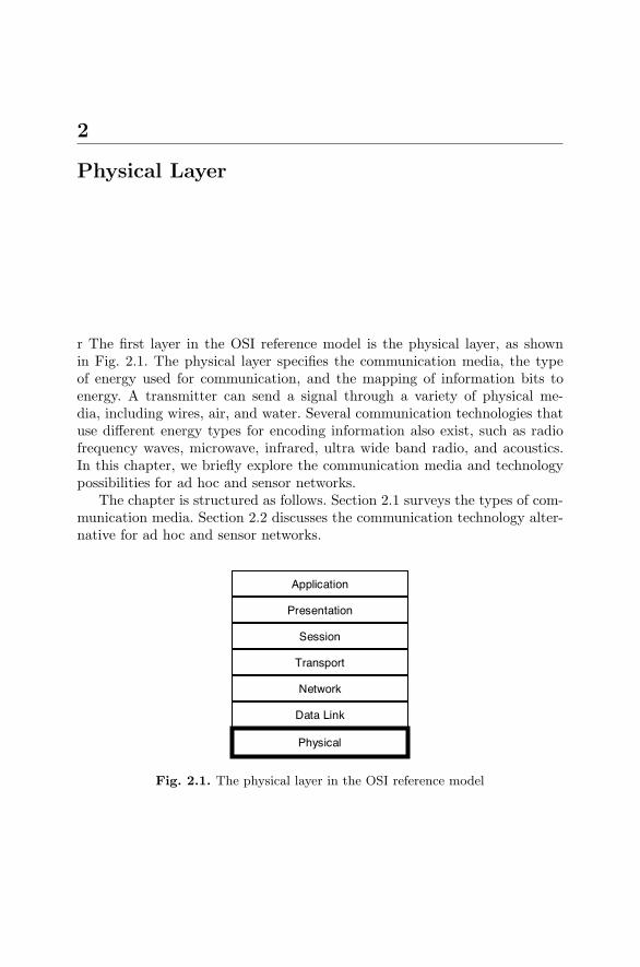
r The first layer in the OSI reference model is the physical layer, as shownin Fig. 2.1. The physical layer specifies the communication media, the typeof energy used for communication, and the mapping of information bits toenergy. A transmitter can send a signal through a variety of physical me-dia, including wires, air, and water. Several communication technologies thatuse different energy types for encoding information also exist, such as radiofrequency waves, microwave, infrared, ultra wide band radio, and acoustics.In this chapter, we briefly explore the communication media and technologypossibilities for ad hoc and sensor networks.
The chapter is structured as follows. Section 2.1 surveys the types of com-munication media. Section 2.2 discusses the communication technology alter-native for ad hoc and sensor networks.
Application
Presentation
Session
Transport
Network
Data Link
Physical
Fig. 2.1. The physical layer in the OSI reference model
8 2 Physical Layer
2.1 Communication Media
The communication medium specifies the physical channel over which signalsare transmitted. Communication media fall into 2 broad categories: wiredcommunications and wireless communications. The remainder of this sectionexplores each category in more detail.
2.1.1 Wired Communication
Wired communications involve signal transmission over a wire or cable. Trans-mitting signals over wires provides a high degree of control over the signalpath, so the quality of signals in wired communications is more stable andrelatively higher than the signal quality of comparable wireless communica-tions.
A common type of wire used for both telephone communication and wiredlocal area networks is the copper twisted pair. Twisted pair cables consist oftwo conducting wires wound around each other in order to reduce electro-magnetic interference, referred to as crosstalk, and a plastic enclosure. Thereare several categories of twisted pair cables that provide different degrees ofsignal quality depending on the number of twists per meter and the shieldingtype. For example, category 3 twisted pair cables typically support lower bitrate voice communication on telephone networks, in the range of Kbits persecond. Category 5 cables support higher speed data transfer for local areanetworks, up to 100 Mbits per second. Shielded versions of category 5 andthe higher grade category 6 cables can support even higher bit transfer rates,making them suitable for Gigabit ethernet networks.
Another type of wire that also supports local area networks is the coaxialcable, which is used as a transmission line to carry a high-frequency or broad-band signal. Coaxial cables consist of a round conducting wire, surrounded byan insulating spacer, surrounded by a cylindrical conducting sheath, usuallysurrounded by a final insulating layer. The magnetic field created betweenthe conducting sheath and conducting wire is used for transmitting broad-band signals, including cable television signals. Coaxial cable is attractive forits relative immunity to outside interference sources, yielding a high signalquality.
The final type of wired communication media we consider is the fibreoptic cable. These cables promise extremely high bit transfer rates because ofthe huge available bandwidth. Fiber optic cables typically serve as long haulcommunication lines for transcontinental communications as well as shorterrange high speed communications.
Wired communication media can serve certain applications of ad hoc andsensor networks. For example, a set of laptops can use category 5 cables toautonomously form an ad hoc network. Similarly, a network of sensors con-nected by wires on the ceiling of a factory can keep track of merchandizemovements. However, wired communication media are not generally suitable
2.1 Communication Media 9
for ad hoc and sensor networks. Despite the higher degree of control and thehigher signal quality for wired communications, this communication mediumlacks the flexibility required by mobile and transient applications that charac-terize ad hoc and sensor networks. In many cases, the mere reliance on wiredcommunications implies the need for installation and deployment of someform of infrastructure, violating the basic premise of ad hoc and sensor net-works. Furthermore, the use of wires severely limits the mobility of a systemby the length of wires. Finally, many ad hoc and sensor network applicationsrequire deployment in situations where wire installation is not practical, suchas disaster relief or environmental monitoring.
The above discussion has shown that wired communications could be use-ful for particular ad hoc and sensor applications, but it is not suitable forthe general application space of these networks. The next section focuses onwireless communications, which overcome many of the drawbacks of wiredcommunications for ad hoc and sensor networks.
2.1.2 Wireless Communication
Wireless communications rely on signal transmission over a medium withoutthe presence of wires or cables between the sender and receiver. Possible com-munication media for wireless communication include air, water, or vacuum.Wireless communications can support a high degree of mobility and deploy-ment flexibility, so they are the main communication medium of choice for adhoc and sensor networks.
The attractive feature of wireless communications, the absence of wires,also presents drawbacks. The absence of a physical wire connecting the senderand receiver render the transmitted signal much more vulnerable to interfer-ences and background noise while traversing the wireless medium. As a result,the expected signal quality of a wireless communication link is relatively lower,less stable, and less predictable than a comparable wired link. The higher vul-nerability to interferences requires higher quality margins and smarter controlof wireless links to maintain communication. Wireless communications arealso inherently less secure than wired communications. An eavesdropper sim-ply needs to capture the wireless signal through an available receiver, whereaslistening in to wired communications requires physically tapping into the com-munication line. The use of wireless communications also complicates higherlayer network functionality, such as the hidden terminal problem at the MAClayer, which is discussed further in Ch. 3. Wireless communications requiremore sophisticated and adaptive mechanisms at several layers of the networkstack.
The flexibility, practicality, and support for mobility of wireless communi-cations overweigh the drawbacks discussed above. The wide scope of potentialapplications for wireless communications, especially in the context of ad hocand sensor networks, warrants the added development and operating cost foradvanced network management mechanisms.
10 2 Physical Layer
This section has covered the potential communication media for ad hoc andsensor networks. The next section explores the communication technologiesthat utilize the medium.
2.2 Communication Technologies
A system’s communication technology specifies the energy type for encodinginformation bits, as well as the methods for encoding information bits intoenergy and decoding them. Examples of communication technologies includeradio frequency, infrared, microwave, laser, ultra wide band radio, and acous-tics. The adoption of different communication technologies stems from thediverse needs of communication applications. For example, microwave and in-frared technologies provide point-to-point links between a sender and receiver,yielding better communication efficiency and signal quality. However, ad hocand sensor network applications may benefit more from broadcast commu-nication technologies, such as radio frequency and ultra wide band radio. Inthis section, we survey the potential communication technologies and theirsuitability for ad hoc and sensor networks. Section 2.2.1 discusses the tech-nologies that typically use point-to-point communication, while Section 2.2.2focuses on broadcast communication technologies.
2.2.1 Point-to-Point Communication Technologies
Point-to-point communication technologies have their roots in many wiredcommunication applications, such as telephone networks or long-distance datatransmission lines. The main purpose of point-to-point communication tech-nologies is to establish a one-to-one communication link between a senderand the intended receiver. Achieving this property through wires is relativelysimple, since wires can physically guide the signal along its designated path.
Point-to-point communication through wireless technologies is a more chal-lenging task. The wireless medium is inherently a broadcast medium in whichthe signal of a wireless transmitter spreads in all outbound directions. Due tothe inherent broadcast nature of many wireless communication technologies,directional antennas are used to guide the transmitter’s signal energy towardsthe receiver. Directional antennas provide a higher signal quality at the re-ceiver by channeling most of the energy in the direction of the receiver. Thedrawback of directional antennas is the higher cost and hardware complex-ity. Even with the use of directional antennas, most wireless point-to-pointcommunication technologies also require an unobstructed line-of-sight (LOS)between the sender and receiver.
Network applications have used certain communication technologies, suchas infrared and microwave signals, for point-to-point wireless communications.Infrared technology encodes information through signals with a wavelengthbetween 750nm and 1mm, the so-called infrared spectrum. For example, many
2.2 Communication Technologies 11
laptops are equipped with built-in infrared ports for interfacing with cellphones and other laptops. When a laptop comes into the vicinity of anotherdevice equipped with infrared communication capability, the two devices canestablish a communication link. The infrared port of the two devices mustbe closely aligned without any physical obstacles between them to ensure aLOS. Another common example of one-way infrared wireless communicationsis television remote controls. The disadvantage of using infrared technologyfor ad hoc and sensor networks, in addition to the LOS requirement, is itssusceptibility to interference from light sources, such as neon lights or sun-light. Furthermore, available infrared transceivers have limited communicationranges within the order of tens of meters, which constrains network range.
Microwave technology uses high frequency radio signals, with wavelengthsranging between 1mm to 30cm. Microwave technology can be either a point-to-point or a broadcast technology. A common application of point-to-point mi-crowave technology is the provision of television signals to subscribers throughsmall dishes for signal transmission and reception. Point-to-point microwaveapplications are highly directive, requiring a careful alignment and mainte-nance of orientation between the sender and receiver. In urban areas, mi-crowave transceivers are generally installed on roofs in order to ensure a LOSfrom an antenna tower, because an obstruction in the LOS severely affectsthe communication.
In general, point-to-point wireless communication technologies require pre-cise positioning and orientation of the transceiver to maintain acceptable com-munication links. This property renders point-to-point technologies suitablefor a small and specific subset of ad hoc and sensor network applications,namely scenarios with limited mobility and highly predictable topologies. Thenext section discusses the class of communication technologies that is moresuitable for ad hoc and sensor networks: broadcast technologies.
2.2.2 Broadcast Communication Technologies
Broadcast communication technologies support the concurrent reception of atransmitted signal by multiple receivers. In contrast to point-to-point tech-nologies that require careful positioning and alignment of the transceivers,broadcast communications can use lower complexity omnidirectional anten-nas that require much less maintenance, so they provide better support forad hoc deployments and mobile networks. The above properties of broadcasttechnologies have made them the top choice for ad hoc and sensor networks.
A related technology is satellite communications through which a networkof artificial satellites orbiting the earth relays earth-based signals. Satellitecommunications currently support telephone, television, radio, scientific, andmilitary applications. Satellites inherently represent infrastructure networks,since satellite deployment involves extensive planning and high deploymentcost for putting the nodes into orbit. In the context of ad hoc and sensornetworks, satellites can serve as the supporting infrastructure for the network.
12 2 Physical Layer
For example, many ad hoc and sensor network design approaches consider thateach network node possesses location information through the satellite-basedGlobal Positioning System (GPS) [4].
One of the more established broadcast communication technologies isthrough radio frequency (RF) waves. Sending radio frequency waves entailsfeeding alternative current to an antenna to produce electromagnetic waves.The RF spectrum includes frequencies from a few hertz to several hundredgigahertz. Applications that use RF technology include radio, television, cel-lular telephones, and radar. A large portion of the current standards that areapplicable for wireless networks, and especially ad hoc and sensor networks,uses RF waves. The popular IEEE 802.11 standard [5], which supports bothcentralized and ad hoc modes for wireless local area networks, relies on RFwaves in both the 2.4 Ghz and the 5 Ghz bands. Similarly, the recent Blue-tooth standard [6] for wireless personal area networks (WPAN) also uses RFwaves in the 2.4 Ghz band.
Many sensor network manufacturers have also adopted RF communica-tion technology. For example, the widely used Crossbow mica motes [7] haveadopted RF communication in the 400Mhz, 900Mhz, and 2.4Ghz bands. Thelatter band satisfies the recent Zigbee [8] standard for sensor networks. Radiofrequency identification (RFID) [9], an emerging technology for replacing barcodes through tiny radio frequency tags, represents another application forRF communication. Chapter 10 covers a case study of an RF sensor network.
Another emerging RF technology is ultra wide band (UWB) radio, aspread-spectrum technique based on the modulation of short nanosecond lowpower pulses [10]. This technology has been used for radar applications forover half a century. In recent years, UWB has received increasing recognitionfor its applicability to short range communication networks because of desir-able features such as high data rates, low power consumption, precise rangingcapability, resistance to multipath fading, and penetration of dense objects.All of the above properties make UWB a strong candidate technology for adhoc and sensor networks. For example, emergency workers using an UWB adhoc network for earthquake recovery could place nodes equipped with sensorsin the rubble to detect signs of living survivors. Because of UWB’s groundpenetrating capability, the nodes in the rubble can effectively communicatewith surface nodes. Chapter 11 presents an example scenario of UWB ad hocnetworks.
Acoustic communication is yet another broadcast technology that has re-cently received increasing attention. Acoustic communication relies on themodulation of acoustic waves with digital data. While acoustics has beenthe technology of choice for underwater communications for over half a cen-tury [11], several projects have demonstrated the usefulness and applicabilityof acoustics for affordable and easily deployable mobile applications withinthe area of ubiquitous computing [13–16]. For instance, many mobile devicescan exploit on-board speakers and microphones to communicate acoustically.Acoustic waves typically have a short communication range, and they do not
2.3 Physical Layer Optimization Parameters 13
penetrate walls, which adds security to the communication. On the downside,the supportable information transfer rate of acoustics is limited by the nar-row acoustic bandwidth. Chapter 12 provides an example of how ad hoc andsensor networks can exploit the low bit rate and short communication rangecapabilities of acoustic communications to form multihop networks.
Broadcast communication has commonly been associated with wirelessmedia, but there are also networks that employ broadcast communicationsover wired media. For example, Ethernet networks that work over category 5cables broadcast signals over wires and through hubs. The broadcast natureof Ethernet necessitates mechanisms at higher layers to avoid collisions.
2.3 Physical Layer Optimization Parameters
This section identifies the relevant parameters at the physical layer, which canbe incorporated into cross-layer design strategies.
2.3.1 Transmission Power
In wireless communications, the transmitter emits signals at a certain powerlevel, which is referred to as the transmission power. The signal loses energyas it propagates from sender to receiver. The so-called signal path loss variesproportionally with dα, where d is the distance between sender and receiver,and α is the path loss coefficient ranging between 2 and 4. The transmis-sion power must be high enough to achieve an acceptable signal quality atthe receiver. However, the transmission power is also upper bounded by reg-ulatory limits and by interference considerations at neighboring transceivers.Transmitters must use a power level within these constraints i.e. a power levelthat is both sufficient to communicate effectively with the receiver and thatadheres to regulatory emission limits. Because the medium conditions in adhoc and sensor networks are highly dynamic, nodes should ideally adapt theirtransmission power continuously to the current conditions. Cross-layer designcan enable interaction between the physical layer and higher layers for bettertransmission power adaptation.
2.3.2 Processing Power
Many of the traditional network protocols do not consider processing powerin determining network behavior. However, processing power can play a sig-nificant role for ad hoc and sensor network protocols. Most ad hoc networksemploy a multihop communication strategy with a short distance per link.For networks with short range wireless links, the processing power becomesnon-negligible relative to the transmission power. While it is difficult to en-force strict processing power control at run-time, consideration of processing
14 2 Physical Layer
power in determining network behavior can improve performance. For exam-ple, some sensor networks support in-network processing. A load balancingstrategy for these sensor networks must consider processing power at eachnode to determine how to distribute the network load evenly. Because loadbalancing typically occurs at higher layers, a cross-layer design strategy isrequired to expose the processing power information to higher layers.
2.3.3 Sensing Power
In sensor networks, the sampling of physical indicators also consumes power,referred to as the sensing power. As for the case of processing, sensing powerbecomes appreciable relative to transmission power for shorter wireless links.For instance, consider a seismic monitoring sensor network in which nodesperiodically sample their sensors to determine if the seismic activity is abovea certain threshold level. If so, then the nodes communicate the sensed datatowards the user. Otherwise, the node continues the periodic sampling of theirsensors until an event occurs. If a long time passes before the occurrence of aseismic event, the network nodes do not consume power due to transmissionsduring that time. However, the nodes do consume sensing power for periodicsampling of the sensors.
2.3.4 Signal-to-Noise Ratio
The signal-to-noise ratio (SNR) is a quality indicator for communication links.The SNR provides a figure of merit through the comparison of the receivedsignal strength with noise level at the receiver. Thus, the SNR is proportionalto the received power and inversely proportional to the sum of the backgroundnoise and interference at the receiver. Stated differently, improving the signalquality at a receiver can be achieved either by increasing the transmissionpower (which causes an increase in the received power) or by reducing back-ground noise and interference. Typically, wireless applications set minimumrequirements for SNR on a network-wide or a per-link basis. In cross-layerdesign, the individual link SNR can serve as an input to a comprehensiveoptimization of node behavior that satisfies the physical layer quality require-ments.
2.3.5 Transmission Rate
The transmission rate indicates the current transfer rate of a communica-tion link. Transmission rates are closely related to the transmission power.Consider an active communication link that satisfies the SNR quality re-quirements. Increasing the link’s rate while maintaining the SNR unchangedrequires an increase in the transmission power. Network mechanisms can ex-ploit this relationship to trade off lower rates for a reduced transmission powerfor rate-elastic traffic. Similarly, nodes can achieve higher transmission ratesthrough an increase in transmission power.
2.3 Physical Layer Optimization Parameters 15
2.3.6 Modulation Code and Rate
Modulation is the process of varying a carrier signal in order to use that sig-nal to convey information. Three basic features of the signal can be variedto carry information: amplitude, frequency, or phase. In addition, modulationtechniques can use a combination of these features. For example, Pulse Posi-tion Modulation (PPM) is a common modulation technique for time-hoppingUWB networks. UWB relies on the regular transmission of nanosecond sig-nals, called monocycles. To encode information, PPM shifts monocycles intime. For example, sending the monocycle 1 ns earlier indicates a zero bit,and delaying the monocycle by 1 ns indicates a one bit. M-ary PPM canalso encode several bits per monocycle, by defining 2M shift positions of themonocycle. The number of bits encoded in each PPM symbol is referred toas the modulation rate. Increasing the modulation rate yields increases in thetransmission rate, but it also lowers the signal quality since it makes it moredifficult for the receiver to decode the signal.
Adaptive cross-layer mechanisms can vary the modulation rate accordingto dynamic medium conditions. For example, if a node observes a rise in theinterference level, it can lower its modulation in order to ensure that thereceiver can still decode the signal.
A common feature of spread-spectrum technologies, such as UWB or CodeDivision Multiple Access (CDMA) [17], is the use of codes to provide signal ro-bustness and security. Spread-spectrum technologies enable concurrent trans-mission through the use of codes that are orthogonal or quasi-orthogonal. Ina network with ongoing links, selecting an appropriate code for a new link canmaximize the rate for the new link and minimize the impact on the perceivedinterference of neighboring nodes.
3
Data Link Layer
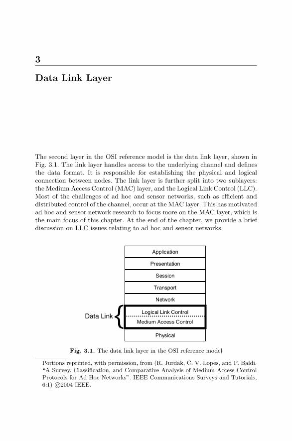
The second layer in the OSI reference model is the data link layer, shown inFig. 3.1. The link layer handles access to the underlying channel and definesthe data format. It is responsible for establishing the physical and logicalconnection between nodes. The link layer is further split into two sublayers:the Medium Access Control (MAC) layer, and the Logical Link Control (LLC).Most of the challenges of ad hoc and sensor networks, such as efficient anddistributed control of the channel, occur at the MAC layer. This has motivatedad hoc and sensor network research to focus more on the MAC layer, which isthe main focus of this chapter. At the end of the chapter, we provide a briefdiscussion on LLC issues relating to ad hoc and sensor networks.
Physical
Application
Presentation
Session
Transport
Network
Logical Link Control
Medium Access Control{Data Link
Fig. 3.1. The data link layer in the OSI reference model
Portions reprinted, with permission, from (R. Jurdak, C. V. Lopes, and P. Baldi.“A Survey, Classification, and Comparative Analysis of Medium Access ControlProtocols for Ad Hoc Networks”. IEEE Communications Surveys and Tutorials,6:1) c©2004 IEEE.
18 3 Data Link Layer
3.1 Introduction
In the OSI reference model, medium access is a function of the layer 2 sublayercalled the Medium Access Control (MAC) layer. MAC protocols for wirelessnetworks must address the hidden node problem (discussed in Sect. 3.2.1)and must exercise power control. Accessing the wireless medium thus requiresmore elaborate mechanisms than wired networks to regulate user access tothe channel. The absence of a centralized controller in wireless ad hoc andsensor networks presents even greater MAC layer challenges than infrastruc-ture wireless networks, creating a need for distributed management protocolsat the MAC layer, and possibly at higher layers of the network stack.
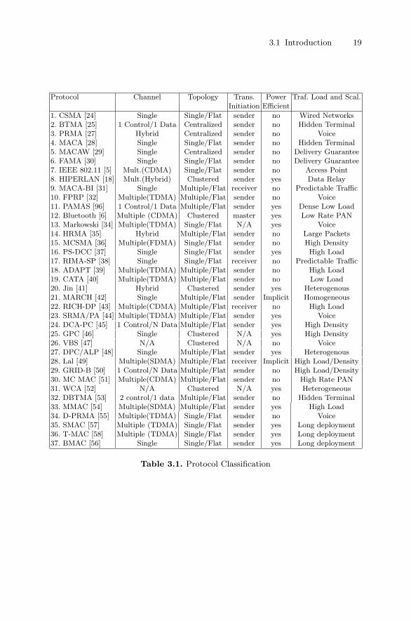
Here, we analyze the features of ad hoc and sensor network MAC protocolsthrough a comprehensive survey of existing MAC protocols, ranging fromindustry standards (IEEE 802.11 [5], Zigbee [8], and Bluetooth [6]) to researchproposals. Table 3.1 shows the list of surveyed MAC protocols for wireless adhoc and sensor networks in chronological order.
Designing improved protocols at the MAC layer requires an understandingof the features that characterize such protocols. From our survey of availableMAC protocols for ad hoc and sensor networks, 5 key features emerge: (1)channel separation and access; (2) transmission initiation; (3) topology; (4)power; and (5) traffic load and scalability. A detailed justification on theselection of these features is available in [179].
3.1.1 Protocol Overview
It is evident from the overview presented above that a variety of design choicescan be made for each feature and application. Combining various designchoices of features involves complex tradeoffs. In addition, most protocolsin Table 3.1 were designed for a specific class of applications or physical layertechnologies, thus trading off generality for efficiency. Here, we analyze thesetradeoffs for the existing protocols, and we further assess the suitability ofvarious combinations of features for ad hoc network and sensor network ap-plications. This tradeoff analysis and the classification of the protocols yieldappropriate design guidelines for general wireless ad hoc and sensor networkMAC protocols.
In the rest of the chapter, each section focuses on one of the protocol fea-tures through a discussion of representative protocols. Note that we drop theterm “wireless” when referring to ad hoc and sensor networks in these sec-tions. Section 3.2 describes existing channel separation and access techniques,which are the central mechanisms of MAC protocols. Section 3.3 focuses onthe transmission initiation feature and discusses the effect that this featurehas on a protocol’s performance and applications.
The subsequent sections discuss the additional features that exploit cross-layer information for improving the performance of ad hoc network and sensor
3.1 Introduction 19
Protocol Channel Topology Trans. Power Traf. Load and Scal.Initiation Efficient
1. CSMA [24] Single Single/Flat sender no Wired Networks2. BTMA [25] 1 Control/1 Data Centralized sender no Hidden Terminal3. PRMA [27] Hybrid Centralized sender no Voice4. MACA [28] Single Single/Flat sender no Hidden Terminal5. MACAW [29] Single Centralized sender no Delivery Guarantee6. FAMA [30] Single Single/Flat sender no Delivery Guarantee7. IEEE 802.11 [5] Mult.(CDMA) Single/Flat sender no Access Point8. HIPERLAN [18] Mult.(Hybrid) Clustered sender yes Data Relay9. MACA-BI [31] Single Multiple/Flat receiver no Predictable Traffic10. FPRP [32] Multiple(TDMA) Multiple/Flat sender no Voice11. PAMAS [96] 1 Control/1 Data Multiple/Flat sender yes Dense Low Load12. Bluetooth [6] Multiple (CDMA) Clustered master yes Low Rate PAN13. Markowski [34] Multiple(TDMA) Single/Flat N/A yes Voice14. HRMA [35] Hybrid Multiple/Flat sender no Large Packets15. MCSMA [36] Multiple(FDMA) Single/Flat sender no High Density16. PS-DCC [37] Single Single/Flat sender yes High Load17. RIMA-SP [38] Single Single/Flat receiver no Predictable Traffic18. ADAPT [39] Multiple(TDMA) Multiple/Flat sender no High Load19. CATA [40] Multiple(TDMA) Multiple/Flat sender no Low Load20. Jin [41] Hybrid Clustered sender yes Heterogenous21. MARCH [42] Single Multiple/Flat sender Implicit Homogeneous22. RICH-DP [43] Multiple(CDMA) Multiple/Flat receiver no High Load23. SRMA/PA [44] Multiple(TDMA) Multiple/Flat sender yes Voice24. DCA-PC [45] 1 Control/N Data Multiple/Flat sender yes High Density25. GPC [46] Single Clustered N/A yes High Density26. VBS [47] N/A Clustered N/A no Voice27. DPC/ALP [48] Single Multiple/Flat sender yes Heterogenous28. Lal [49] Multiple(SDMA) Multiple/Flat receiver Implicit High Load/Density29. GRID-B [50] 1 Control/N Data Multiple/Flat sender no High Load/Density30. MC MAC [51] Multiple(CDMA) Multiple/Flat sender no High Rate PAN31. WCA [52] N/A Clustered N/A yes Heterogeneous32. DBTMA [53] 2 control/1 data Multiple/Flat sender no Hidden Terminal33. MMAC [54] Multiple(SDMA) Multiple/Flat sender yes High Load34. D-PRMA [55] Multiple(TDMA) Single/Flat sender no Voice35. SMAC [57] Multiple (TDMA) Single/Flat sender yes Long deployment36. T-MAC [58] Multiple (TDMA) Single/Flat sender yes Long deployment37. BMAC [56] Single Single/Flat sender yes Long deployment
Table 3.1. Protocol Classification
20 3 Data Link Layer
MAC protocols. Section 3.4 examines the effect of incorporating topology in-formation on the MAC protocol performance. Section 3.5 assesses availablepower management mechanisms and their suitability for particular channelaccess methods and topologies. Section 3.6 evaluates the scalability and per-formance of MAC protocol design choices. Section 3.8 offers a roundup of adhoc and sensor network MAC issues and derives guidelines for creating a moregeneralized protocol that is suitable for several physical-layer technologies andapplications.
3.2 Channel Separation and Access
A key factor in the design of a MAC protocol for ad hoc and sensor networks isthe way in which it utilizes the available medium. Earlier approaches assumeda common channel for all stations, while more recent approaches have usedmultiple channels for more efficient use of the medium.
In this section, we explore both single channel and multiple channel MACprotocols. Furthermore, we classify multiple channel protocols based on theirchannel separation mechanism. Within each channel separation strategy, wedescribe the channel access method of particular protocols.
3.2.1 Single Channel
Considering the medium as a single channel was the most prominent ap-proach in the earlier years of MAC design [24, 26, 28–30], primarily becausemechanisms for channel separation had not yet been developed. In a commonchannel MAC protocol, all the nodes in the network share the medium for alltheir control and data transmissions. Collisions are an inherent attribute ofsuch protocols. Two stations that transmit simultaneously will both fail, anda back-off mechanism is required by both stations.
The first proposed single channel protocol is Carrier Sense Multiple Ac-cess (CSMA) [24]. In CSMA, a node senses the common channel for ongoingtransmissions. If the channel is idle, it begins its transmission. Otherwise, itsets a random timer before attempting to transmit again. CSMA does not ad-dress the handling of collisions on the channel. An improved variant of CSMAis CSMA/CD [26] (CSMA with collision detection). In CSMA/CD, if two ormore transmissions collide, the sending nodes are notified and each chooses arandom time before retransmitting. If a node detects a collision for the secondtime, it backs off for twice the time it backed off the last time. This mech-anism is known as Binary Exponential Back-off (BEB). The performance ofCSMA protocols degrades quickly with high load, due to increased frequencyof collisions and increased transmission latency.
When applying CSMA to networks where some nodes are not within rangeof each other, two or more nodes may have a common neighbor while theyare out of range. If both nodes sense the channel and try to transmit to this
3.2 Channel Separation and Access 21
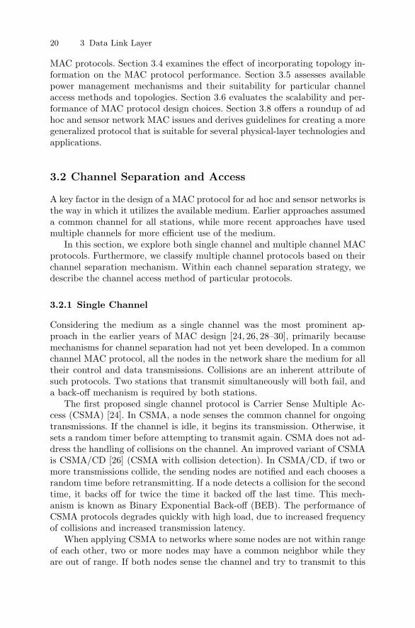
common neighbor, then a collision occurs. Figure 3.2 illustrates this situa-tion, which is called the hidden node problem. Multiple Access with Collision
Fig. 3.2. The Hidden Node Problem: Node A senses the medium as idle and initiatesa transmission to node B. Node C also senses the medium as idle and initiates atransmission to node B. A collision occurs at node B, and both A and C are unawareof the collision since they are out of each other’s range
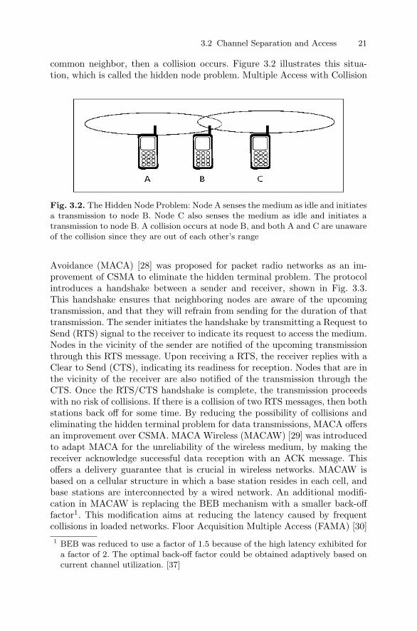
Avoidance (MACA) [28] was proposed for packet radio networks as an im-provement of CSMA to eliminate the hidden terminal problem. The protocolintroduces a handshake between a sender and receiver, shown in Fig. 3.3.This handshake ensures that neighboring nodes are aware of the upcomingtransmission, and that they will refrain from sending for the duration of thattransmission. The sender initiates the handshake by transmitting a Request toSend (RTS) signal to the receiver to indicate its request to access the medium.Nodes in the vicinity of the sender are notified of the upcoming transmissionthrough this RTS message. Upon receiving a RTS, the receiver replies with aClear to Send (CTS), indicating its readiness for reception. Nodes that are inthe vicinity of the receiver are also notified of the transmission through theCTS. Once the RTS/CTS handshake is complete, the transmission proceedswith no risk of collisions. If there is a collision of two RTS messages, then bothstations back off for some time. By reducing the possibility of collisions andeliminating the hidden terminal problem for data transmissions, MACA offersan improvement over CSMA. MACA Wireless (MACAW) [29] was introducedto adapt MACA for the unreliability of the wireless medium, by making thereceiver acknowledge successful data reception with an ACK message. Thisoffers a delivery guarantee that is crucial in wireless networks. MACAW isbased on a cellular structure in which a base station resides in each cell, andbase stations are interconnected by a wired network. An additional modifi-cation in MACAW is replacing the BEB mechanism with a smaller back-offfactor1. This modification aims at reducing the latency caused by frequentcollisions in loaded networks. Floor Acquisition Multiple Access (FAMA) [30]1 BEB was reduced to use a factor of 1.5 because of the high latency exhibited for
a factor of 2. The optimal back-off factor could be obtained adaptively based oncurrent channel utilization. [37]
22 3 Data Link Layer
Fig. 3.3. RTS/CTS handshake: Node A requests access of the channel through theRTS. Node B replies with a CTS indicating that it is ready to receive node A’stransmission. Node C receives a CTS from node B and thus refrains from transmit-ting for the duration indicated in CTS. Even though A and C are hidden from eachother, the handshake ensures that a collision at node B does not occur
enhances MACAW by adding carrier sensing before sending a RTS. MACA-BI (By invitation) [31] takes a receiver-initiated approach, where a receiverindicates its readiness to receive by broadcasting a Ready to Receive (RTR)message. Any neighbor that hears a RTR can then send data to any destina-tion. Therefore, MACA-BI does not prevent collisions in the vicinity of thereceiver.
Receiver Initiated Multiple Access with Simple Polling (RIMA-SP) [38]improves on MACA-BI by allowing polled neighbors to send only to the pollingnode. RIMA-SP also allows both nodes to send data after the handshake iscomplete. In both MACA-BI and RIMA-SP, the receiver takes a proactive rolein initiating transmissions. Transmission initiation will be discussed furtherin section 3.3.2.
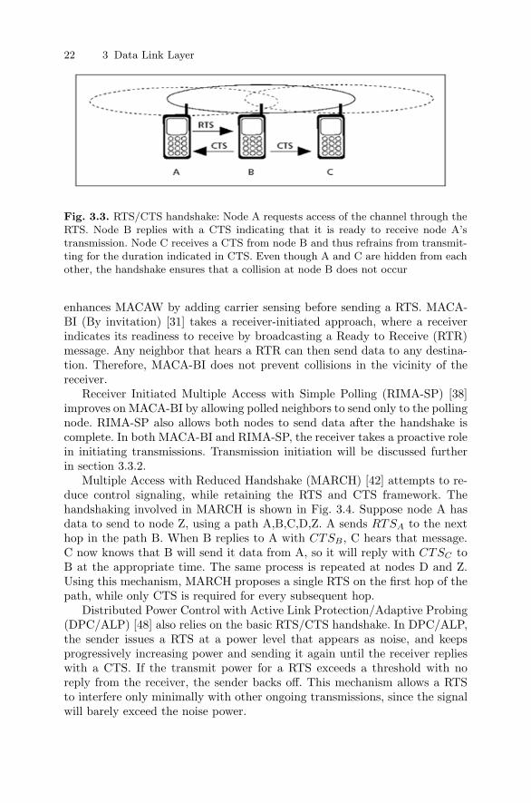
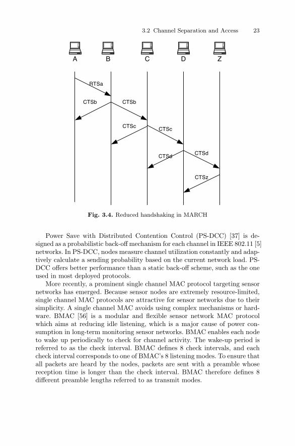
Multiple Access with Reduced Handshake (MARCH) [42] attempts to re-duce control signaling, while retaining the RTS and CTS framework. Thehandshaking involved in MARCH is shown in Fig. 3.4. Suppose node A hasdata to send to node Z, using a path A,B,C,D,Z. A sends RTSA to the nexthop in the path B. When B replies to A with CTSB , C hears that message.C now knows that B will send it data from A, so it will reply with CTSC toB at the appropriate time. The same process is repeated at nodes D and Z.Using this mechanism, MARCH proposes a single RTS on the first hop of thepath, while only CTS is required for every subsequent hop.
Distributed Power Control with Active Link Protection/Adaptive Probing(DPC/ALP) [48] also relies on the basic RTS/CTS handshake. In DPC/ALP,the sender issues a RTS at a power level that appears as noise, and keepsprogressively increasing power and sending it again until the receiver replieswith a CTS. If the transmit power for a RTS exceeds a threshold with noreply from the receiver, the sender backs off. This mechanism allows a RTSto interfere only minimally with other ongoing transmissions, since the signalwill barely exceed the noise power.
3.2 Channel Separation and Access 23
CTSb CTSb
CTSc
CTSd
CTSc
CTSd
CTSz
RTSa
A B C D Z
Fig. 3.4. Reduced handshaking in MARCH
Power Save with Distributed Contention Control (PS-DCC) [37] is de-signed as a probabilistic back-off mechanism for each channel in IEEE 802.11 [5]networks. In PS-DCC, nodes measure channel utilization constantly and adap-tively calculate a sending probability based on the current network load. PS-DCC offers better performance than a static back-off scheme, such as the oneused in most deployed protocols.
More recently, a prominent single channel MAC protocol targeting sensornetworks has emerged. Because sensor nodes are extremely resource-limited,single channel MAC protocols are attractive for sensor networks due to theirsimplicity. A single channel MAC avoids using complex mechanisms or hard-ware. BMAC [56] is a modular and flexible sensor network MAC protocolwhich aims at reducing idle listening, which is a major cause of power con-sumption in long-term monitoring sensor networks. BMAC enables each nodeto wake up periodically to check for channel activity. The wake-up period isreferred to as the check interval. BMAC defines 8 check intervals, and eachcheck interval corresponds to one of BMAC’s 8 listening modes. To ensure thatall packets are heard by the nodes, packets are sent with a preamble whosereception time is longer than the check interval. BMAC therefore defines 8different preamble lengths referred to as transmit modes.
24 3 Data Link Layer
3.2.2 Multiple Channels
Some protocols for ad hoc and sensor networks separate the control and dataplanes by assigning one channel for control signaling, and one or more separatechannels for data transmissions. In this section, we focus on multiple chan-nel protocols and we classify protocols according to their channel separationtechniques.
Generalized Separation
Some multiple channel protocols describe a generalized channel separationscheme. Busy Tone Multiple Access (BTMA) suggests having a separate busytone channel to solve the hidden terminal problem of CSMA, where a cen-tralized base station sensing the data channel as busy can place a sine waveon the busy tone channel to prevent any nodes from transmitting. A recentextension of using busy tones was presented in Dual Tone Busy Tone MultipleAccess (DT-BTMA), where two out-of-band busy tone channels are used toprotect RTS transmission, and to prevent nodes in the receiver’s vicinity fromtransmitting. It therefore focuses on solving the hidden terminal problem in asimilar way to BTMA, while using a distributed approach rather than a basestation. Power Aware Multiple Access with Signaling (PAMAS) proposes us-ing one control channel for sending RTS/CTS, and a separate data channel.In terms of handshaking, PAMAS uses the same sequence as MACA. PAMASalso specifies that nodes that detect RTS or CTS refrain from communicatingfor the duration indicated in the overheard control messages.
Dynamic Channel Assignment with Power Control (DCA-PC) is anothergeneralized channel separation protocol having one control and N data chan-nels. In DCA-PC, a sender checks if any of the data channels appear free. Ifso, it chooses one of the available channels and sends a RTS signal on thecommon control channel with maximum power to the destination. If the des-tination agrees on the sender’s channel choice with no conflict, it replies withCTS at a power level appropriate to reach the sender, and then the sender canreserve the channel. If the destination has a conflict with the sender’s channelchoice, the destination’s free channel list is sent to the sender so that it canchoose a more appropriate channel.
Another generalized channel separation protocol is Grid with Channel Bor-rowing (GRID-B), which proposes initially assigning channels to each cell ina predefined geographic area. Highly loaded cells would borrow channels fromneighboring lightly loaded cells if needed. Negotiations for such lending wouldoccur on a common control channel. GRID-B proposes the use of Code Divi-sion Multiple Access (CDMA) or Frequency Division Multiple Access (FDMA)for channel allocation. In the case of CDMA, channel bandwidths are fixedand therefore increasing the number of channels up to a certain limit is quitebeneficial. In FDMA, the total bandwidth is fixed, and therefore having ad-ditional users would reduce the per user bandwidth.
3.2 Channel Separation and Access 25
Time Division Multiple Access
Time Division Multiple Access (TDMA) segments the medium into severalfixed time frames that are subdivided into slots. To ensure that nodes keeptrack of time frames and slots, TDMA protocols must maintain synchroniza-tion among the nodes. In these protocols, only one station may transmit duringa particular time slot. Because of their periodic nature, TDMA protocols aremost suitable for real-time and deadline sensitive traffic.
The first proposed TDMA protocol for ad hoc networks is the Five PhaseReservation Protocol (FPRP) [32], in which each slot is split into an informa-tion slot and reservation slot. A sender that wants to reserve an informationslot must contend for it during its reservation slot. The reservation slot consistsof five phases that resolve conflicts among all nodes that are also contendingfor the information slot within a two-hop radius. A node that reserves an in-formation slot can transmit with a low chance of collisions during that slot.In FPRP, nodes maintain perfect synchronization through GPS.
Collision Avoidance Time Allocation (CATA) [40] adopts almost the sameconcept as FPRP, with the only distinction of using four reservation mini-slots to access a slot instead of five. Soft Reservation Multiple Access withPriority Assignment (SRMA/PA) [44] also resembles FPRP, since they bothshare the notion of having several mini-slots to reserve a data slot. The addedfeature in SRMA/PA is that it classifies nodes into high and low-prioritynodes, where high-priority nodes can grab reserved slots from low-prioritynodes. Categorizing nodes in this manner gives better performance for voicenodes in the network. The protocol also suggests a new back-off mechanism,where access probability is based on packet laxity.
Markowski [34] proposed a window splitting protocol based on TDMA.This protocol classifies nodes according to their traffic classes: Hard RealTime (HRT), Soft Real Time (SRT), and Non Real Time (NRT). Each classof nodes can preempt nodes in lower classes. Furthermore, nodes are onlyallowed to transmit at the beginning of a slot, while all nodes maintain perfectsynchronization. Within each class, collisions are resolved through a windowsplitting mechanism. If a collision occurs for two nodes of the same class, thenhalf of the nodes of that class are placed in an active window for the currentslot, while the other half are placed in an inactive window. Nodes in the activewindow contend for the next slot. If collisions occur again, the active windowis further split into an active and an inactive window. Window splitting isdone on Node ID basis for HRT, on packet laxity for SRT, and on arrival timefor NRT. There is no specification of how to handle synchronization in thisprotocol, nor is there any reference to the hidden node problem.
ADAPT [39] proposes assigning slots to nodes to cope with high load andhigh density networks. It also suggests using contention to manage the unusedslots. Each active node owns one slot and is given priority to send RTS in itsslot while other nodes listen for the owner’s transmission. If the owner doesnot send a RTS during its own slot, other nodes will contend for this slot
26 3 Data Link Layer
by trying to send their own RTS. At that point, a node that receives a CTSmessage may use this slot only in the current frame.
In Distributed Packet Reservation Multiple Access (D-PRMA) [55], whichis an adaptation of PRMA (see Section 3.2.2), nodes are designated as voiceor data terminals. Only voice terminals can reserve the same slot for subse-quent frames. This resembles slot ownership in ADAPT with the distinctionthat only voice terminals may temporarily own slots. A slot is split into mmini-slots, and contention in the first mini-slot determines the winner in theslot. If there are collisions in the first mini-slot, nodes contend again for theslot during the second mini-slot, and so on. Voice terminals are given pri-ority over data terminals by always contending through the first mini-slots.Synchronization in D-PRMA is achieved through GPS.
There are also TDMA-based MAC protocol that are specifically designedfor sensor networks. Sensor MAC (S-MAC) [57] is a heavyweight MAC pro-tocol for sensor networks that relies on time synchronization and schedulingamong nodes to enforce periodic sleep and listen schedules. S-MAC uses threenovel techniques to reduce energy consumption and support self-configuration:
1. To reduce energy consumption in listening to an idle channel, nodes peri-odically sleep. Neighboring nodes form virtual clusters to auto-synchronizeon sleep schedules.
2. S-MAC also sets the radio to sleep during transmissions of other nodes.Unlike PAMAS, it only uses in-channel signaling.
3. S-MAC applies message passing to reduce contention latency for sensornetwork applications that require store-and-forward processing as datamove through the network.
A more recent version of S-MAC [190] has introduced adaptive duty cyclesby enabling a node to snoop on neighbors’ RTS and CTS messages in orderto schedule its own wake-up time. Because nodes have to maintain neigh-bors’ schedules, S-MAC is complex and not sufficiently scalable for large scalenetworks of resource-limited nodes.
T-MAC [58] also proposes adaptive duty cycles to address the nonuniformtraffic patterns in sensor networks. T-MAC is similar to S-MAC in its essence,but it introduces early sleeping to enable nodes that are scheduled to be activeto go into sleep mode if they are idle. T-MAC suffers from similar complexityand scaling problems of S-MAC, because it trades off a short active time forreduced adaptivity to changing network conditions.
Frequency Division Multiple Access
FDMA splits the available medium into several frequency channels to allowmultiple nodes to transmit simultaneously. A proposed FDMA protocol usesCSMA on each of the frequency channels (MCSMA) [36]. Each node keepsa list of free channels, and when it has data to transmit, it tries to use thechannel that it used during the last transmission. If that channel is busy,
3.2 Channel Separation and Access 27
it selects one of the other free channels. Although MCSMA reduces overallcollisions when compared to original CSMA, collisions and hidden terminalproblems are still present on each channel.
Code Division Multiple Access
CDMA uses one of several orthogonal codes to spread each sender’s signal.Through its use of orthogonal codes, CDMA allows concurrent multiple trans-missions using all of the available spectrum. Multi-code MAC (MC MAC) [51]uses CDMA by assigning N codes for data transmission and one common codefor control signaling. A sending node in MC MAC issues a RTS to anothernode on the common control channel indicating the code(s) that it will use fortransmission. If it gets a CTS it assumes that there is no code conflict withthe intended receiver, and it subsequently sends data after which it expectsan ACK. If the receiver detects code conflicts, it exchanges its usable codeswith the sender, so the sender chooses the appropriate codes for transmission.
IEEE 802.11 [5] Distributed Coordination Function (which is the specifi-cation for infrastructureless mode in Wireless Ethernet) is almost identical toMACAW on each of its channels, except that it combines a CSMA mechanismwith MACAW to lower the probability of RTS collisions. IEEE 802.11 splitsthe medium by using one of two forms of CDMA, either Frequency HoppingSpread Spectrum (FHSS), or Direct Sequence Spread Spectrum (DSSS). InFHSS, it allows up to 79 different hopping channels in North America and Eu-rope, thus supporting up to 26 co-located networks. In DSSS, IEEE 802.11buses 12 codes to allow concurrent transmissions of nodes. In IEEE 802.11,nodes that hear RTS or CTS set their Network Allocation Vector (NAV),which indicates the remaining time until a current channel becomes free. Thestandard also provides a busy channel which nodes can sense to check if themedium is idle. To promote fairness among nodes and to prevent large trans-mission latencies, IEEE 802.11 introduces a contention window from whichnodes waiting to transmit choose a random back-off time. The size of thecontention window adapts to the number of collisions that occur. A node maytransmit once its back-off timer expires. Whenever a node is forced to waitthrough another frame, it continues counting down from where it stopped in-stead of choosing a new random waiting time. This ensures that nodes thatwait longer get priority to access the medium.
Receiver Initiated Channel Hopping with Dual Polling (RICH-DP) [43]combines the slow frequency hopping aspect of HRMA [35] and the receiverinitiation aspect of RIMA/SP [38] to allow nodes to reserve hops and to senddata both ways once a hop is reserved. A receiver that is ready to receive datasends a RTR message to its neighbors. If some neighbor has data to send, itresponds with a RTS to reserve the hop for data exchange between the pair.Both nodes can send data once they complete this reservation.
28 3 Data Link Layer
Space Division Multiple Access
Like in CDMA, Space Division Multiple Access (SDMA) aims at using thefull spectrum all of the time to a certain degree. In SDMA, nodes use di-rectional antennas thus allowing a node to begin a transmission at any timeas long as that the transmission’s direction does not interfere with an ongo-ing transmission. In Lal’s [49] SDMA protocol, a node polls neighbors withan omnidirectional RTR message that contains the node’s training sequence.A training sequence indicates the directions in which a node accepts trans-missions. Nodes that have data to send reply to the polling node using adirectional RTS (DRTS) that contains each node’s own training sequence.The polling node then replies to the accepted senders with a Directional CTS(DCTS) to complete the handshake. The use of directional antennas can there-fore accommodate concurrent multiple senders to the polling node.
MMAC [54] proposes a technique of using smart antennas to establish mul-tihop link through the RTS/CTS handshake. In MMAC, nodes keep profiles ofthe neighboring transceiver directions. Whenever a new data request arrivesat the MAC layer, the MAC initiates carrier sensing in the direction of theintended receiver. If the channel is idle in that direction, the MAC then issuesa directional RTS to the next hop in the path to the destination. Nodes on thepath to the destination forward this RTS message directionally until the RTSreaches its destination. The destination then replies with CTS directly to thesender, and the two establish data communication. Neighboring nodes thatfall within the range of this new directed link set their Directional NetworkAllocation Vector (DNAV) for the duration of the transmission.
Hybrid Protocols
Hybrid protocols combine two or more of the above approaches. Packet Reser-vation Multiple Access (PRMA) [27], which was designed for an infrastruc-ture network to enable voice nodes to communicate alongside data nodes, usesboth TDMA and FDMA. PRMA divides time into frames that are further seg-mented into slots, and each slot may be either reserved or unreserved. Thereis also one upstream and one downstream frequency channel. A sender has tolisten for an unreserved slot, to contend for it using ALOHA, and to await abase station’s decision on the winner for this slot. PRMA also classifies nodesas periodic and non-periodic traffic nodes. If a periodic traffic node reservesa slot, that node can use the same slot in subsequent frames.
High Performance Local Area Network (HIPERLAN) [18], which is theEuropean counterpart of IEEE 802.11, uses another hybrid FDMA/TDMAchannel access scheme. It provides a maximum of five frequency channels,each with a rate of 23.5 Mbps. Furthermore, nodes have to contend for thechannel in three phases prior to reserving it. The length and structure of thesephases are based on fixed time slots and frames.
3.3 Transmission Initiation 29
Hop Reservation Multiple Access (HRMA) [35] is another hybrid of TDMAand FDMA. In HRMA, nodes are all synchronized and hop to a commonsequence (each slot, all the nodes listen to the same frequency, and switchto another frequency during the next slot). If a node has data to send, itsends a Hop Reservation (HR) message using the current frequency hop, andit follows that with a RTS message to the intended receiver. If the receiverreplies with CTS, then the pair has reserved the current frequency hop andthey can send any amount of data using that frequency, while all other nodesare still following the common hopping sequence.
Jin [41] proposes a hybrid CDMA/TDMA protocol, where nodes dynami-cally elect a Pseudo Base Station (PBS) based on power considerations. ThePBS maintains synchronization and assigns codes to nodes that it manages,using frames that have 3 mini-slots for synchronization, reservation, schedul-ing, in addition to the data slot.
Bluetooth [6] also combines CDMA and TDMA. A master node in Blue-tooth assigns frequency hopping sequences a piconet, which allows simulta-neous communication between the master and up to seven slaves. Bluetoothuses time division duplexity to separate the uplink and downlink. The masternode manages medium access through a polling and reservation scheme, andit also assigns hopping sequences and maintains synchronization within thepiconet.
3.2.3 Channel Separation and Access Summary
Many medium access protocols for ad hoc networks use a variant of theRTS/CTS handshake. Protocols that do not use this handshake rely on carriersensing, periodic exchanges of information among nodes, or reservations. Mul-tiple channel protocols, which use different techniques for channel separation,generally allow for more users than single channel protocols.
3.3 Transmission Initiation
Some protocols adopt a sender-initiated approach to transmissions; others se-lect a receiver-initiated approach. The choice of a transmission initiation strat-egy depends on the protocol’s target application types. Historically, sender-initiated protocols were most common until recently. In the rest of this section,we discuss each of the two approaches, and we categorize protocols based ontheir transmission initiation strategy.
3.3.1 Sender-Initiated
CSMA [24] was the first sender-initiated protocol, with the sender sensing thechannel before transmitting. Many protocols that followed, such as MACA [28]
30 3 Data Link Layer
and IEEE 802.11 DCF [5], adopted the RTS/CTS mechanism to overcome thehidden node problem in CSMA. The RTS/CTS handshake became a basis formany proposed protocols to come. This handshake is based on the assumptionthat senders should be the proactive entity in establishing communication, byindicating their intent to transmit data. This handshake was also adopted inmany multiple channel protocols to contend for and reserve available channels.For example, PRMA [27], FPRP [32], and MC MAC [51] use a sender-initiatedhandshake on a common control channel to attempt to reserve a particulardata channel. Sender-initiated approaches are more intuitive and more suitedto generalized networks with unpredictable traffic patterns.
3.3.2 Receiver-Initiated
In this class of protocols, receivers poll their neighbors with a RTR message,which indicates a node’s readiness to receive data. The first such protocol isMACA-BI [31], which was primitive in nature. In MACA-BI, a node sendsRTR to its neighbors whenever it is ready to receive data. A polled node thathas data to send can subsequently transmit to any node, not necessarily thepolling node. MACA-BI is suitable for certain sensor network applicationsthat require sending data in certain directions regardless of node identities.
RIMA-SP [38] adds the restriction to MACA-BI that nodes can only sendto the polling node, and that both nodes can send data once the handshake iscomplete. In RICH-DP [43], receivers use RTR to poll neighbors, but they doso to reserve the current frequency hop. RICH-DP also adds an ACK messagethat is issued by the receiver when it successfully receives a portion of data.Finally, Lal [49], combines SDMA with a receiver-initiated approach, wherea receiver sends RTR omnidirectionally and awaits directional RTS messagesfrom potential senders.
A receiver-initiated MAC protocol yields better network performance fora specific class of ad hoc networks. In sensor networks, for example, the goalis to get data to a certain data sink. The particular source node of the datamay not be important, as long as the data is from a certain region of thenetwork. In this case, having a receiver poll its nodes for any available data isdesirable. In networks where nodes have data to send often, a receiver-initiatedapproach also performs well since most RTR messages serve a useful purpose.This approach also has its shortcomings. By merely announcing its readinessto receive data, a receiver does not ensure that exactly one of the neighboringnodes will attempt to send data. Therefore, more recent protocols proposeadditional mechanisms such as frequency hop reservation or directional RTSmessages to mitigate this problem.
3.3.3 Transmission Initiation Summary
The appropriate transmission initiation strategy of a protocol is highly de-pendent on the potential application areas of that protocol. For generalized
3.4 Topology 31
networks, a sender-initiated protocol is more suitable. For some specializednetworks, such as sensor networks, receiver-initiated protocols are a betterchoice.
3.4 Topology
Although topology is primarily network layer aspect, certain protocols usetopology information for making better decisions at the MAC. Exploitingtopology-related information at the MAC layer is an example in which cross-layer design can enhance performance.
Ad hoc and sensor networks may include nodes with varying capabilitiesand resources. Nodes may also be mobile, so the topology of an active networkcould change frequently. Therefore, an efficient protocol is one that assumes atopology as generalized as possible. The network must also be able to adaptto heterogeneous node capabilities in a way that optimizes performance andminimizes energy consumption. Network topology can typically be describedin terms of hierarchy and hops. A network could have a centralized, clustered,or flat topology. In the centralized case, a single node or base station controlsand manages all other nodes in the network. Clustered topologies designateone node in each group of nodes to handle localized central control of thegroup. Flat topologies consider a fully distributed approach, where all nodesare both nodes and routers, and the notion of centralized control is absent.
We make a further characterization of protocol topologies by examiningthe hop nature of a network. Some protocols assume that nodes only needto communicate with reachable neighbors, and are referred to as single hopprotocols. Other protocols assume that nodes need to communicate beyondtheir reachable neighbors, and that sometimes a packet has to be relayedthrough many intermediate nodes to get to its destination. We refer to theseprotocols as multihop. Single hop protocols are simple but restrictive sincethey offer limited support for larger networks. Multihop protocols are moregeneral in scope and more scalable, although they introduce added complexityinto channel access mechanisms.
There are several combinations of hierarchy and hops in proposed proto-cols: (A) single hop flat topology; (B) multiple hop flat topology; (C) clusteredtopology; and (D) centralized topology. This section categorizes protocols ac-cording to their topology and explores how each topology choice impacts anetwork’s performance.
3.4.1 Single Hop Flat Topology
Single Hop Flat Topology protocols are not concerned with handling relayingof data, and consider that all nodes are similar in capabilities. Some proto-cols [24,28,30,31,38,56] assume that a node has a global view of the network,or that higher layer protocols can handle reaching distant nodes. Thus, each
32 3 Data Link Layer
node only has to contend with its immediate neighbors in order to obtain ac-cess of a channel. As the node density and network load increase in a network,these protocols scale poorly since delay increases exponentially and through-put drops drastically. Other protocols [5,34,35,55] attempt to add scalabilityand adaptability to harsh network conditions to this topology class, either byproviding multiple channels to support an increased number of users [5,55], orby offering techniques such as window splitting and hop reservation [34,35,43]to make better use of the common medium.
In dense or highly loaded networks, however, capacity and performanceare limited in a single hop topology, even when using optimization techniques.Other drawbacks of a single hop topology are high power consumption andlack of flexibility. For instance, when two nodes move away from each other,both must increase their transmit power if they still need to communicate.Even if transmit power adaptation is ensured, the price for mobility is in-creased average power consumption, which could have been avoided in a mul-tihop topology. Therefore, this topology is more suited for wired networks orsmaller scale and lower throughput wireless networks, such as Personal AreaNetworks (PAN) or sparse Local Area Networks (LAN).
3.4.2 Multiple Hop Flat Topology
Multiple Hop Flat Topology protocols offer a more scalable and general ap-proach. Protocols that use this topology also consider that the network ishomogeneous in terms of node capability and functionality. Ad hoc and sen-sor networks can benefit from a multihop topology mainly in power efficiencyand correct channel reservation mechanisms beyond one-hop neighbors.
PAMAS [96] addresses the possibility of some nodes being out of rangeof the receiver or transmitter, and it allows nodes within range of an activetransmission to turn off their radios for power efficiency.
Some multiple channel protocols [36,51] also exploit a multihop flat topol-ogy to allow for spatial reuse of channels within the network, thus increasingthe total number of allowable hosts. Had they been implemented in a singlehop topology, these protocols would have only been able to support as manynodes as there are frequency channels.
Other protocols [32, 39, 40, 44, 51, 190] consider that nodes can only reachtheir immediate neighbors, but they also have to establish reservations thatdo not conflict within their two-hop neighborhood. In a single hop topology,channel reservation in these protocols would have to be unique among allnodes, thus preventing any channel reuse.
Some multiple hop flat topology protocols [45, 48] not only make use ofmultihop for channel access, but also for limiting the overall power consump-tion by forcing nodes to transmit only with the power necessary to reach thereceiver. Because of their multihop topology, nodes may choose to send data
3.4 Topology 33
through a multihop path to a node that is within transmission range 2. Theseprotocols show how a multihop topology can reduce overall power consump-tion in the network. Through the use of directional antennas, MAC proto-cols [49, 54] can direct the emitted power toward the receiver, enabling moreactive multihop links to coexist on the same channel.
3.4.3 Clustered Topology
One major challenge in ad hoc networks is performing network initiation, man-agement and control. In infrastructure networks, a base station handles thesefunctions. Researchers have found the idea of centralized control attractive,and have tried to emulate it in ad hoc and sensor network models by design-ing protocols that use a clustered topology. In a clustered topology, one nodeamong each group of nodes is selected to act as the cluster head. Clusteredtopology protocols attempt to reduce control overhead at individual nodes byplacing much of this burden at the cluster head. There are several approachesto choosing the cluster head.
In small sensor networks, the choice of a cluster head is static. Typically,one node, known as the gateway node, has the capability of communicatingwith the sensor nodes as well as a larger network such as the Internet. If all thenodes are within range of the gateway node, then the cluster head is alwaysthe gateway node.
In other networks, the selection of a cluster head can be dynamic. TheVirtual Base Station (VBS) [47] protocol focuses on a dynamic random se-lection of a virtual base station for clusters in mobile networks. In VBS, eachnode announces its IP address periodically by sending “hello” messages to itsneighbors. Nodes listen to “hello” messages and join the cluster of the low-est IP address node in their vicinity. Changes in the network such as nodesmoving or dying are adapted to through the periodicity of “hello” messages.Although VBS protocol provides a simple mechanism for choosing a uniquecluster head in a specific area in the network, the selection of a cluster headis totally random (since IP addresses do not hold any information relating tonodes). Furthermore, VBS has the undesirable feature that nodes with lowerIP addresses suffer from resource overuse.
TDMA-based sensor network MAC protocols [58,190] also implement thevirtual cluster model in order to enable nodes to keep their clocks synchro-nized. By electing cluster heads periodically and listening to cluster headbeacons, nodes can compensate any local clock skews.
An approach that addresses some of the shortcomings of virtual base sta-tions is the Weighted Clustering Algorithm (WCA) [52]. WCA algorithm pro-poses electing cluster heads based on a weight function at each node thatexpresses a node’s suitability for being a cluster head. In WCA, nodes first2 [175] describes techniques for deciding when to use a multihop path instead of a
single hop path through power considerations.
34 3 Data Link Layer
discover their neighbors, including node degrees, distances and velocities. Anode’s degree is the number of neighbors that it has. After this initial discoveryphase, each node calculates and announces its own weight value. The param-eters that contribute to the weight function are: the distance from neighbors(for transmit power consideration); the time a node will spend as a clusterhead (battery power available); mobility; and connectivity. The algorithm alsoproposes that cluster heads of different clusters maintain connections to eachother using dual power radios. Finally, WCA supports mobile nodes by allow-ing handovers for nodes moving from one cluster to another.
Similar protocols [41,46] propose electing a cluster head according to bat-tery power only, which is a simpler but less generalized approach than WCA.Electing cluster heads based on battery power is suitable for large sensor net-works, where energy consumption is a critical issue because of the limitedenergy resources at each node. Nodes that are far from the gateway node canthus elect a cluster head based on battery power.
Bluetooth [6] also has a clustered topology in the form of piconets of onemaster and up to seven active slaves. The master is not dynamically chosen,rather it is always the initiator or founder of the piconet. Since Bluetooth wasdesigned for Personal Area Networks (PAN), which aim at achieving wirelessconnections within an office or home, such a selection of the master makessense. A PC or another central device generally has to be powered on, andthat device polls less intelligent devices to establish connections. For other adhoc networks with more general applications, statically assigning a master isinefficient.
HIPERLAN [18] is another standard that adopts a clustered topology. Inthis protocol, some nodes are designated as forwarders, which are responsiblefor relaying data to distant nodes. HIPERLAN designates other nodes as P-supporter nodes to keep track of the sleep schedule of neighboring nodes (seeSection 3.5.2). Therefore, in HIPERLAN, forwarders and P-supporters sharethe duties of a cluster head.
3.4.4 Centralized Topology
Centralized topology protocols [25, 27, 29] require the presence of a centralbase station to coordinate medium access. For instance, in BTMA, all nodescommunicate through the base station, which sends an out-of-band busy sig-nal whenever the data channel is busy to prevent collisions. In PRMA, nodescontend for available time slots in the next frame. A central base station de-termines the status of each slot in the next frame and announces the successfulreservations for the upcoming frame. Finally, MACAW assumes that there areseveral fixed base stations connected with a wired network.
Ad hoc and sensor networks generally do not adopt a centralized topology,since by definition they are infrastructureless. However, these protocols pro-vide valuable concepts such as a busy tone channel and time slot reservationwhich are extendable to ad hoc and sensor networks.
3.5 Power 35
3.4.5 Topology Summary
In short, multihop flat topology or a clustered topology are more suitable toensure scalability in ad hoc and sensor networks. Both of these topologies re-quire more control messaging. In homogeneous networks, a multiple hop flattopology is more appropriate for balancing network loads. In heterogeneousnetworks, a clustered topology allows the high power nodes to become clus-ter heads and handle most of the overhead control messaging. A single hoptopology requires fewer control messages but it is not scalable. A centralizedtopology is by definition an infrastructure network, and thus it is not an optionfor ad hoc networks.
3.5 Power
A major design consideration for ad hoc and sensor network MAC protocolsis the power consumption of individual nodes, and the overall power con-sumption of the network. Power consumption at the nodes stems from datatransmission and reception, idle listening to the channel, processing, sleeping,sensing, or actuating. Power consumption is an inherently cross-layer aspect,since some of the above power sinks, such as processing and sensing, are notMAC layer functions. This section reveals how ad hoc and sensor networkMAC protocols can exploit cross-layer power-related information for optimiz-ing performance.
Power conservation is important for any type of mobile node, whether op-erating in an ad hoc or infrastructure network, because of its limited batterypower. In infrastructure networks, a resourceful base station is responsible formanaging channel access and allocation, while nodes consume most of theirpower for data transmissions. In ad hoc and sensor networks, however, theabsence of a base station places the burden of control on one or more of thenodes. Furthermore, the absence of a centralized controller increases chances ofcollisions and channel assignment conflicts that lead to higher power consump-tion in the form of control signaling and retransmissions. Sensor networks areparticularly sensitive to the issue of power consumption because nodes mustendure long deployment with the limited available energy resources.
Because the medium access strategy significantly impacts energy consump-tion of a mobile node, we can achieve much of the power optimization in adhoc and sensor networks through careful design of the MAC protocol. In thissection, we describe common mechanisms for power conservation, and we clas-sify protocols based on the mechanisms they adopt.
3.5.1 Transmit Power Control
A major cause of power consumption at a node is transmission power, a physi-cal layer parameter. MAC protocols that operate on transmission power adopt
36 3 Data Link Layer
a form of cross-layer interaction between the MAC and physical layers. Someprotocols [45,46] have proposed controlling the transmit power so that it is justenough to reach the intended receiver. For example, DCA-PC specifies thateach node continuously monitors, records and updates the transmission powerlevel it needs to reach each neighbor. In DCA-PC, a node is initially unawareof the appropriate power levels, so it transmits with maximum power. Onceit establishes contact with a neighbor, then both nodes learn the appropriatepower levels they need to communicate.
DPC/ALP [48] is another protocol that supports transmission power con-trol. Recall that in DPC/ALP, a node sending its RTS progressively increasesits transmit power until it exceeds a threshold of detection at the receiver.If the receiver replies, then a connection is established, otherwise the senderbacks off. During data transmissions, a sender in DPC/ALP also transmits atthe minimum power needed to overcome noise at the receiver.
Lal [49] and MMAC [54] exercise another method of power control throughdirectional antennas. Because nodes send messages in the direction of theintended receiver, the transmission requires less power than in the omni-directional case, where the signal is scattered in all directions.
Some protocols propose power control enhancements to the IEEE 802.11MAC protocol [154, 234]. These protocols specify that a sender and receivertransmit RTS and CTS control messages at maximum power so that neighborsbecome aware of the upcoming transmission. The sender can subsequentlytransmit the data at a lower power level which is directly related to the dis-tance between the pair of nodes, instead of the maximum power level. Thework in [233] has shown that this approach may produce asynchronous linksand that it may lead to collision in the carrier sensing zone of the sender.Reference [233] proposes that the sender and receiver periodically raise thepower level during the sending of data to keep neighbors within the carriersensing zone aware of the ongoing transmission.
Transmission power control benefits dense or highly loaded networks,where a large number of nodes need to efficiently share the wireless mediumwith minimal interference. Protocols that support this mechanism must alsouse few data channels to avoid overuse of the common control channel.
3.5.2 Sleep Mode
Some protocols acknowledge that in ad hoc and sensor networks, a consid-erable portion of power consumption is wasted due to overhearing irrelevanttransmission, or due to idle listening to the channel. PAMAS [96] takes advan-tage of the simple RTS/CTS handshake to avoid this problem. As mentionedearlier, PAMAS has a common control channel and a common data channel.Nodes that hear RTS or CTS on the control channel refrain from communi-cating since they are in the neighborhood of either the sender, receiver, orboth. These neighboring nodes power off their transceivers for the durationof the transmission indicated in the handshake messages. Therefore, PAMAS
3.5 Power 37
reduces battery power consumption in highly connected low load networks,where at any time, many idle nodes overhear other nodes’ transmissions.
HIPERLAN [18] also allows nodes to go into sleep mode to conserve power.Such nodes are called p-savers, and must set up a specific wake-up pattern bynotifying specialized neighboring nodes called p-supporters. P-supporters areresponsible for keeping track of the sleep schedules of neighboring p-savers,for buffering data for these nodes, and for forwarding it to them when theyare set to wake up. This mechanism obviously requires extra buffer space andbattery resources at p-supporter nodes.
Bluetooth [6] supports three low-power states: Park, Hold, and Sniff. Parkstate provides the lowest duty cycle and thus the lowest energy consumption.In this state, a node releases its MAC address but remains synchronized withthe piconet. The node wakes up occasionally to synchronize and listen forbroadcast messages. Hold state is the next higher low-power state. In Holdstate, a node keeps its MAC address and transmits immediately after wakingup. Finally, in the Sniff state, a node listens to the piconet more often thanin the Hold state, but still at a lower rate than normal. The rate at which anode listens is programmable and application-dependant.
Sleep modes are especially useful in sensor networks. Sensor network de-ployments could span several months or years. For much of that deploymenttime, the nodes wait for events to happen in the environment and they donot transmit any data. Consequently, nodes should power down their radiosto avoid wasting energy for idly listening to the channel. BMAC [56] enforcessleep modes through the definition of asynchronous check intervals. BMACempowers each node to set the frequency at which to wake up its radio tocheck for channel activity. Other sensor network MAC protocols [58,190] relyon synchronization and snooping on neighbors’ control messages for determin-ing wake-up times.
The use of sleep modes involves an inherent tradeoff between energy con-sumption and delay in ad hoc and sensor networks. Nodes that wake up lessoften save energy, but they also incur more delay for data delivery. Long-term sensor network monitoring applications favor this tradeoff, since energyconsumption is the main concern in these applications. On the other hand,this tradeoff may not be suitable for real-time applications, such as voice orvideo transfer through an ad hoc network. Another potential drawback ofsupporting sleep modes is the overhead power consumption for powering upand powering down a transceiver. In some cases, this overhead may exceed thepower savings of supporting sleep mode. Therefore, whether it is beneficial tosupport sleep mode depends on the specifications of particular transceivers.
3.5.3 Battery Level Awareness
There are several protocols that are aware of battery power levels at nodes andadjust their behavior accordingly. A common strategy is to base the selectionof a cluster head on battery levels. DPC/ALP and Jin also classify nodes
38 3 Data Link Layer
into High Power (HP) and Low Power (LP) according to remaining batterypower. DPC/ALP gives LP nodes priority during transmissions, by allowingthem to reserve slots sooner than HP nodes. All of these protocols producepower savings when they are used in a power heterogeneous network. Forexample, a network may include laptops, palmtops, and pens equipped withtransceivers. One of the laptops would generally be selected as a cluster headbecause of its relatively high power resources. For similar reasons, electronicpens get priority for transmission in DPC/ALP due to their limited batterypower.
WCA [52] also considers battery power along with several other parametersto elect a cluster head. Because it combines the effects of several factors inelecting a cluster head, WCA performs well in both power homogeneous orheterogeneous networks.
A form of battery level awareness can also promote power savings in sensornetworks. Although the battery level of a sensor node is a critical factor,measuring the absolute battery level of a sensor node is inaccurate becauseof fluctuations in voltage. Instead, sensor nodes can make use of a relativeindicator of battery level, such as the node’s radio duty cycle during the pasttime window [192]. Nodes could use this relative measure of battery level foradapting MAC behavior, such as setting the radio duty cycle dynamically.
3.5.4 Reduced Control Overhead
The exchange of control messages prior to data transmission is also a sourceof power waste. Whereas control messages are necessary to avoid collisions,reducing these messages to the minimum is beneficial. MARCH [42] is oneprotocol that follows this reasoning. As described earlier, in a path where thereare N hops, MARCH uses 1 RTS message and N CTS messages. When N islarge, power savings from this approach are considerable. However, MARCHignores the case of heterogeneous power nodes. Referring to Fig. 3.4, when anode A has data to send to another node Z, using the path A-B-C-D-Z, Asends RTSA to node B. B replies with CTSB to indicate to A that it is readyto receive data. MARCH assumes that the next node in the path C hearsCTSB when it was sent to A. In this assumption, MARCH supposes that allnodes are equidistant in the network, and that nodes are always transmittingat a constant power level. If transmit power control was used in conjunctionwith MARCH, then the mechanism does not work. For example, C might befurther away from B than A, in which case C does not hear CTSB .
3.5.5 Savings for Particular Settings
Given that different networks have varying particularities when it comes topower, some protocols focus on achieving power savings for specific settings.One of these protocols, SRMA/PA [44], is concerned with quality of service
3.5 Power 39
and considers that there are high and low priority traffic. It allows high pri-ority traffic to preempt the low priority traffic when trying to grab slots fortransmission. Markowski’s [34] protocol follows a similar reasoning for threetraffic classes. This technique improves performance for high priority traffic,but it has the opposite effect for lower priority traffic. In a network with manyvoice or real-time traffic nodes, both protocols reduce overall network powerconsumption by avoiding collisions and retransmissions for real-time traffic.
3.5.6 Increased Control Overhead
There are some protocols that are strictly separated from power issues, andtherefore do not incorporate power considerations into their behavior. A fewof these protocols, however, contain power wasting features. For example, theapproach of RICH-DP [43] is suitable for networks with predictable and peri-odic traffic. In networks that do not fit this description, many RTR messagesare sent while no nodes have data to send. In such networks, RTR messagespresent two causes of power waste. The first is the transmit power of the nodesending a non-useful RTR. The second source of power waste is due to idlelistening to RTR messages at neighboring nodes.
TDMA-based protocols also contain a regular source of power waste tomaintain synchronization. Some of these protocols [32,55] assume that nodeshave a GPS radio to maintain synchronization. Although GPS is effective andreliable for keeping nodes synchronized, GPS radios consume valuable bat-tery power resources at each node when periodically receiving synchronizationmessages. Nodes using a CSMA [24] protocol also waste power through idlelistening to a busy channel.
In all multiple channel protocols with a flat topology, channels are assigneddynamically at each node. This represents control overhead and thereforewasted power for performing channel assignments. In these protocols, nodestypically need to monitor different channels for availability, or to adopt agreedy approach in grabbing channels. Monitoring channels dictates that thenode’s transceiver is frequently active thus wasting more power. In a greedyapproach, the chance of conflicts and collisions is increased since a node triesto grab channels that may already be used. A clustered topology typicallyreduces the chance of conflicts by limiting the number of nodes contendingfor channels and by assigning a portion of the control tasks to a cluster head.
3.5.7 Power Summary
The extent to which each of the different power saving mechanisms in thissection actually conserves power is dependent on the application scenario. Amulti-purpose protocol should enable the selection and tuning of a wide varietyof power-saving mechanisms for different application scenarios, without addingoverhead that would counterbalance the benefits of having these features.
40 3 Data Link Layer
3.6 Traffic Load and Scalability
A majority of the surveyed protocols perform well for their intended appli-cations. In this section, we examine the quality of service classes served bythe available MAC protocols: (A) high load; (B) high density; (C) real-timetraffic; (D) long-term operation and (E) more selective scenarios. For eachtraffic load or type, we assess the scalability and adaptability of protocolsto dynamic network conditions. Our discussion of performance is qualitative,based on parameters such as channel utilization, throughput, and delay. Notethat quality of service is an inherently cross-layer aspect that incorporatesindicators from several layers.
3.6.1 Highly Loaded Networks
Receiver-initiated approaches operate well in networks where channel utiliza-tion is high. Since nodes send RTR messages whenever they are ready toreceive data, there is a high probability that whenever a sender has data, itcan find an appropriate receiver to relay its data. RICH-DP and Lal’s SDMAprotocol both reserve channels (one does so in space and the other does itin frequency) for data transmission once the handshake is complete. As a re-sult, these two protocols exhibit reduced collisions and increased efficiency.Both of these protocols are highly adaptive to varying network conditions,and both offer mobility support. Lal’s SDMA approach is especially effectiveat bottleneck nodes, where support for simultaneous multiple transmissionsis desirable.
PS-DCC [37] also adapts well to high network load. Because it always cal-culates the sending probability based on current channel utilization, PS-DCCreduces collisions in the network when utilization is high by forcing individualnodes to wait for longer durations before transmitting. This technique clearlyintroduces increased transmission latency. If it is used with other channelseparation mechanisms, this scheme becomes attractive in its simplicity andeffectiveness. PS-DCC is also adaptive to the general network case, wherenodes are moving around and topology changes are frequent.
GRID-B [50] is designed to manage areas in the network where the loadis high, which are referred to as hot spots. By adaptively borrowing chan-nels from a neighboring area, a hot spot can support the required load.ADAPT [39] is another protocol designed to handle high load networks, sinceit allocates slots to each node statically. Borrowing of unused slots allowsnodes with a high traffic rate to have increased access to the channel. NeitherGRID-B nor ADAPT are adaptive to a rapidly changing network topology orto highly mobile nodes due to their static assignments of resources. In GRID-B, high mobility might bring nodes out of the predefined geographic area forwhich the channels were initially assigned. Similarly in ADAPT, each slot hasa predefined owner. New nodes that enter the network do not own any slot
3.6 Traffic Load and Scalability 41
and thus have a reduced priority, since they are only allowed to contend forother nodes’ slots.
TDMA protocols (see Sect. 3.2.2) are generally adaptive to highly loadednetworks with periodic traffic, such as a voice-dominated network. These pro-tocols, however, do not cope well with random data traffic, and are not scal-able, since increased network size requires more nodes to contend for a fixednumber of slots.
3.6.2 Dense Networks
Protocols that perform best for dense networks base their behavior on powerconsiderations. Through transmission power control, GPC [46] and DCA-PC [45] limit the possibility of collisions among nodes. DCA-PC performswell in high mobility situations, as well as for larger networks. The only con-straint on DCA-PC is to use few data channels in each vicinity and few powerlevels to avoid control channel overuse. As for GPC, it dynamically choosesforwarding agents based on battery power level, which avoids overusing theresources of a single node and thus promotes fairness in a dense network.
MAC protocols that use directional antennas [49, 54] also perform well indense networks. Although these protocols are appropriate for both high loadand dense networks, which seems attractive, some issues about the economicfeasibility of SDMA remain unresolved. For example, the use of directional an-tennas for sensor networks is questionable because of the hardware complexityand cost of directional antennas. GRID-B handles dense networks through itshot spot mechanism in the same way it adapts to high load situations.
MCSMA [36] also offers a solution for dense but lightly loaded networksthrough its use of several frequency channels that are spatially reused withinsmall distances. In a dense MCSMA network, the per node bandwidth isreduced but the overall channel utilization of the network is increased.
3.6.3 Voice and Real-Time Traffic
Some protocols are more suited for voice and real-time traffic. These protocolstypically have 2 common attributes: priorities and reservations. To supportpriorities, a protocol must classify nodes or traffic into two or more classes.Each class typically has a certain priority level based on node features andnature of traffic. Reservations are usually allowed for higher priority traffic.PRMA [27] was designed to support voice communication in a data networkover the wireless medium. By allowing voice nodes to reserve slots for sub-sequent frames, PRMA ensures that once a voice node reserves a slot, it isguaranteed the needed bandwidth to maintain an acceptable quality of service.This protocol offers improved performance over pure TDMA, but it assumesthere is a base station to maintain synchronization and resolve contentions.An improved adaptation of PRMA for ad hoc networks could be achieved byimplementing it within a clustered topology, where a cluster head performs
42 3 Data Link Layer
most base station functions. D-PRMA [55] adds a fully distributed flavor tothe original PRMA, by having nodes resolve contention for slots among them-selves. D-PRMA performs well for periodic traffic networks. SRMA/PA [44]follows a similar approach to PRMA, by designating nodes as voice and dataterminals. Since it allows voice nodes to preempt data nodes, SRMA/PA fa-vors voice nodes even more than PRMA. SRMA/PA also performs well in anetwork with many voice terminals.
VBS [47] is another protocol designed for voice and real-time traffic. Af-ter it is elected in a cluster, the VBS allocates virtual circuits to nodes thatrequest connections. Virtual circuits ensure a certain bandwidth allocation,which makes them suitable for supporting real-time traffic. The VBS protocolexhibits stable performance when it comes to VBS changes and cluster mem-berships. It also provides a mechanism for handovers between neighboringclusters which supports mobility. However, this protocol focuses mainly onmanaging topology and clusters, and does not elaborate sufficiently on datatransmission and related issues.
Markowski’s window splitting protocol [34] is also favorable towards real-time traffic, by allowing hard real-time nodes to preempt soft real-time nodesthat also preempt non real-time nodes. Because of its fully distributed nature,the window splitting scheme can theoretically handle a large number of nodesof each traffic class. An increased number of senders, however, causes the activewindow to become too small, and that in turn causes increased transmissionlatency for many nodes. Thus, this protocol performs well in real-time trafficnetworks that are sparse and limited in size. It can also enforce a firm real-time traffic class, where a node attempts to send a packet for a few times assoft real-time, and if those attempts are unsuccessful, then it sends the packetas hard real-time.
3.6.4 Unattended Long-Term Operation
Sensor network deployment could last for several months or even years. Assuch, unattended long-term network operation is a major goal for many sen-sor network MAC protocols. The main challenge in supporting unattendedlong-term operation is making efficient use of the limited energy resources ateach node. BMAC, SMAC, and TMAC all try to efficiently manage the radioduty cycle at each node in order to minimize energy consumption at eachnode. All three protocols acknowledge that idle listening on the radio channelcontributes significantly to node power consumption. As such, these protocolspropose techniques for reducing idle listening by placing radios into low-powerstates when there is no data to transmit or receive.
3.6.5 More Selective Scenarios
There is a group of protocols that performs best when used in more specificsituations, other than traffic deadline restrictions. For example, HRMA [35]
3.7 Logical Link Control 43
performs well when packet sizes are large. Its performance degrades, however,when node density increases. In Jin’s proposed protocol [41], low power nodesget priority over high-power nodes. In a dense network with a large percent-age of low-power nodes, high-power nodes may experience large transmissiondelays. However, if a network only has a few low-power nodes, high-powernodes experience tolerable transmission delays.
MC MAC [51] also has specific constraints for adequate performance. Al-though the number of usable codes is around 30, MC MAC proposes an opti-mal performance for a 7 code network, to avoid overusing the control channel.The protocol also performs best for short range applications. In MC MAC, ahighly loaded network also causes a high access delay.
Ad hoc and sensor networks require versatile and flexible MAC protocols,so protocols that perform well for more selective scenarios are unattractivefor widespread adoption in general ad hoc and sensor networks.
3.6.6 Traffic Load and Scalability Summary
In short, multiple channel protocols and power-efficient protocols exhibitbetter performance for high load and high density networks. TDMA andreservation-based protocols perform best for networks dominated by voiceand real-time traffic. Long-term sensor networks benefit from MAC protocolsthat efficiently manage the radio duty cycle. Protocols that perform well forselective scenarios are not suitable for a general ad hoc network.
3.7 Logical Link Control
The Logical Link Control (LLC) layer lies above the MAC layer and is re-sponsible for performing three main functions:
1. Managing frames to upper and lower layer: LLC provides an interfacebetween the MAC sublayer and layer 3, the network layer, by performingpacket encapsulation and decapsulation.
2. Error control: LLC enforces error control through mechanisms such aschecksums and parity bits. The two forms of possible errors are bit errorsand frame errors. Bit errors indicate errors in a number of bits in a frame.Frame errors indicate badly synchronized or badly received frames.
3. Flow control: LLC defines the data values used in flow control signalingbetween two transmitting hosts, although the actual flow control occursat layer 4.
While managing frames to upper and lower layers happens internally to anode, both error control and flow control involve interaction with other nodes.Many protocols retransmit a frame whenever the receiver detects an error.While retransmission increases a network’s reliability, it also may have adverse
44 3 Data Link Layer
effects on channel utilization, energy consumption, and delay in the network,particularly on higher layers in the network stack.
The following example demonstrates these adverse effects. A network thatuses the Transmission Control Protocol (TCP) [109] usually enforces conges-tion control at layer 4 in order to deal with network congestion. A sendermonitors a receiver’s acknowledgement messages in order to adjust its trans-mission rate. If the sender detects a congestion in the network because ofdelayed acknowledgements, the sender drops its transmission rate by half tohelp reduce congestion. In many cases in wireless networks, the delayed ac-knowledgements may arise because of transmission errors rather than conges-tion. The sender in this case would still drop the transmission rate to alleviatecongestion.
This example shows one of the drawbacks of strict layering. Because thetransport layer is unaware of the cause of the delayed acknowledgements, italways assumes the cause is congestion. Cross-layering could help mitigatethis issue by enabling the transport and LLC layers to share information.Whenever the transport layer misses receiver acknowledgements, it checksthe LLC state to decide whether the missed acknowledgements are due toerrors or congestion. Subsequently, the transport layer could make the rightflow control decision.
3.8 Conclusion and Discussion
Ad hoc and sensor networks provide a distributed communications paradigmthat can be extended to fit into the “anytime anywhere” concept of ubiq-uitous computing [23]. One major obstacle that impedes the proliferation ofsuch networks is the tight regulation exercised on unlicensed communications,restricting frequency bands and bandwidth where ad hoc networks may beused. Whether this distributed model will be applied to a broader range ofnetworks and become dominant in the coming years remains to be seen. Thiswill also depend in part on regulatory issues. The other challenge towardsthe development of ad hoc networks is the design of efficient self-managementprotocols. In our survey of ad hoc and sensor network MAC protocols, it hasbecome evident that the overwhelming majority of these protocols were de-rived heuristically and were aimed at optimizing a particular set of measuresunder a particular set of operating conditions. However, most of these heuris-tics lacked generality and were not tested in a deployed network. Establishinga principled framework for optimizing ad hoc and sensor network behavior ischallenging since there is clearly a wide range of applications and potentialphysical layer technologies that have different considerations.
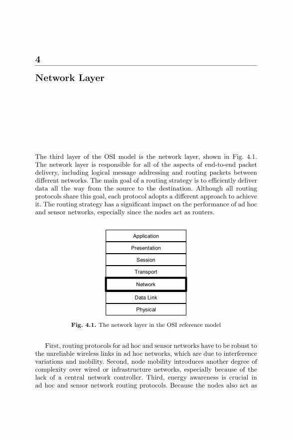
4
Network Layer
The third layer of the OSI model is the network layer, shown in Fig. 4.1.The network layer is responsible for all of the aspects of end-to-end packetdelivery, including logical message addressing and routing packets betweendifferent networks. The main goal of a routing strategy is to efficiently deliverdata all the way from the source to the destination. Although all routingprotocols share this goal, each protocol adopts a different approach to achieveit. The routing strategy has a significant impact on the performance of ad hocand sensor networks, especially since the nodes act as routers.
Application
Presentation
Session
Transport
Data Link
Physical
Network
Fig. 4.1. The network layer in the OSI reference model
First, routing protocols for ad hoc and sensor networks have to be robust tothe unreliable wireless links in ad hoc networks, which are due to interferencevariations and mobility. Second, node mobility introduces another degree ofcomplexity over wired or infrastructure networks, especially because of thelack of a central network controller. Third, energy awareness is crucial inad hoc and sensor network routing protocols. Because the nodes also act as
46 4 Network Layer
routers in ad hoc and sensor networks, energy depletion of some nodes couldmean loss of connectivity in the network.
A characterizing feature of routing protocols is the manner in which theydisseminate routing state among the nodes. The topology of a routing proto-col also impacts performance related to energy efficiency, delay, and through-put. For example, a clustered topology protocol may save energy at mostnodes while incurring more delay for cluster formation. Routing protocols alsoadopt either a connection-oriented approach or a connectionless approach.Connection-oriented communication, such as phone communication, estab-lishes a predefined path for communication between two nodes, similar totrains in the transportation industry. Connectionless communication, such asInternet traffic, routes data on a hop-by-hop basis, resembling the decisionsthat car drivers make at each intersection between the source and destination.
In addition, cross-layer design enables ad hoc and sensor network routingprotocols to exploit information from other layers, providing the followingfeatures:
• Power-Awareness: Efficient power management at ad hoc and sensornetworks’ nodes requires power-aware mechanisms at every layer. Power-aware routing protocols incorporate energy-related metrics into routingcost computation and path selection.
• Location-Awareness: With the availability of positioning systems suchas GPS, location-awareness is an integral part of many routing protocolsfor ad hoc and sensor networks. In most cases, location information en-ables routing protocols to make quicker and more focused decisions forestablishing optimal paths.
• Quality-of-Service: There is a wide range of quality-of-service require-ments for ad hoc and sensor networks, including throughput, delay, re-liability, or energy consumption. Most routing protocols involve tradeoffsbetween these QoS metrics. As a result, several routing protocols for ad hocand sensor networks adopt flexible mechanisms for tuning QoS variablesto support various applications.
This chapter is not intended as a comprehensive survey of existing routingprotocols for ad hoc and sensor networks. Instead, we refer to existing routingprotocols to uncover the strengths and weaknesses of routing protocol designchoices for ad hoc and sensor networks. For comprehensive reviews on routingprotocols for ad hoc and sensor networks, we suggest the surveys in [59,60,181].
The remainder of the chapter is structured as follows. Section 4.1 dis-tinguishes the different classes of routing protocols according to their statedissemination policy. Section 4.2 explores the effect of topology choices on theperformance of routing protocols. A related topological choice is whether touse multipath routes, which we discuss in Section 4.3. Sections 4.4 through 4.6examine proposed routing enhancements for ad hoc and sensor networks thatcut through the traditional layered approach by using information from other
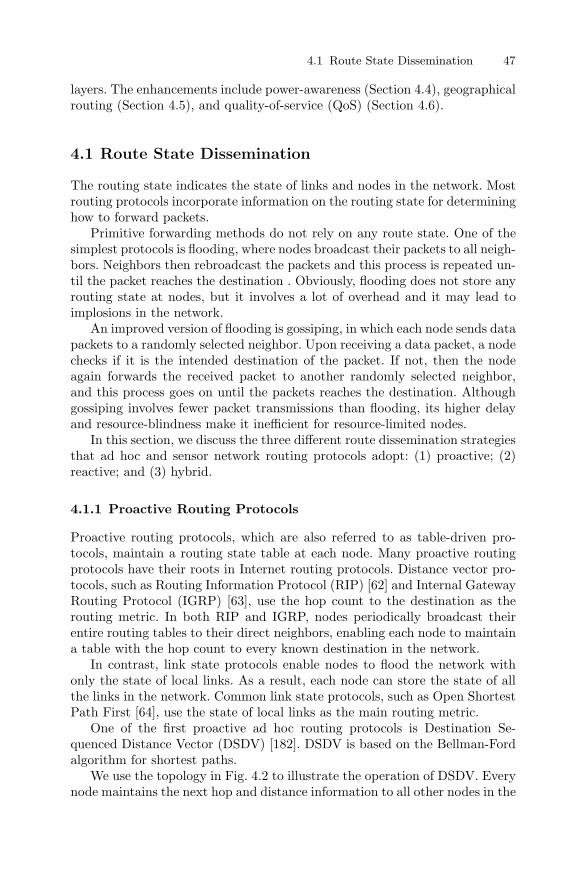
4.1 Route State Dissemination 47
layers. The enhancements include power-awareness (Section 4.4), geographicalrouting (Section 4.5), and quality-of-service (QoS) (Section 4.6).
4.1 Route State Dissemination
The routing state indicates the state of links and nodes in the network. Mostrouting protocols incorporate information on the routing state for determininghow to forward packets.
Primitive forwarding methods do not rely on any route state. One of thesimplest protocols is flooding, where nodes broadcast their packets to all neigh-bors. Neighbors then rebroadcast the packets and this process is repeated un-til the packet reaches the destination . Obviously, flooding does not store anyrouting state at nodes, but it involves a lot of overhead and it may lead toimplosions in the network.
An improved version of flooding is gossiping, in which each node sends datapackets to a randomly selected neighbor. Upon receiving a data packet, a nodechecks if it is the intended destination of the packet. If not, then the nodeagain forwards the received packet to another randomly selected neighbor,and this process goes on until the packets reaches the destination. Althoughgossiping involves fewer packet transmissions than flooding, its higher delayand resource-blindness make it inefficient for resource-limited nodes.
In this section, we discuss the three different route dissemination strategiesthat ad hoc and sensor network routing protocols adopt: (1) proactive; (2)reactive; and (3) hybrid.
4.1.1 Proactive Routing Protocols
Proactive routing protocols, which are also referred to as table-driven pro-tocols, maintain a routing state table at each node. Many proactive routingprotocols have their roots in Internet routing protocols. Distance vector pro-tocols, such as Routing Information Protocol (RIP) [62] and Internal GatewayRouting Protocol (IGRP) [63], use the hop count to the destination as therouting metric. In both RIP and IGRP, nodes periodically broadcast theirentire routing tables to their direct neighbors, enabling each node to maintaina table with the hop count to every known destination in the network.
In contrast, link state protocols enable nodes to flood the network withonly the state of local links. As a result, each node can store the state of allthe links in the network. Common link state protocols, such as Open ShortestPath First [64], use the state of local links as the main routing metric.
One of the first proactive ad hoc routing protocols is Destination Se-quenced Distance Vector (DSDV) [182]. DSDV is based on the Bellman-Fordalgorithm for shortest paths.
We use the topology in Fig. 4.2 to illustrate the operation of DSDV. Everynode maintains the next hop and distance information to all other nodes in the
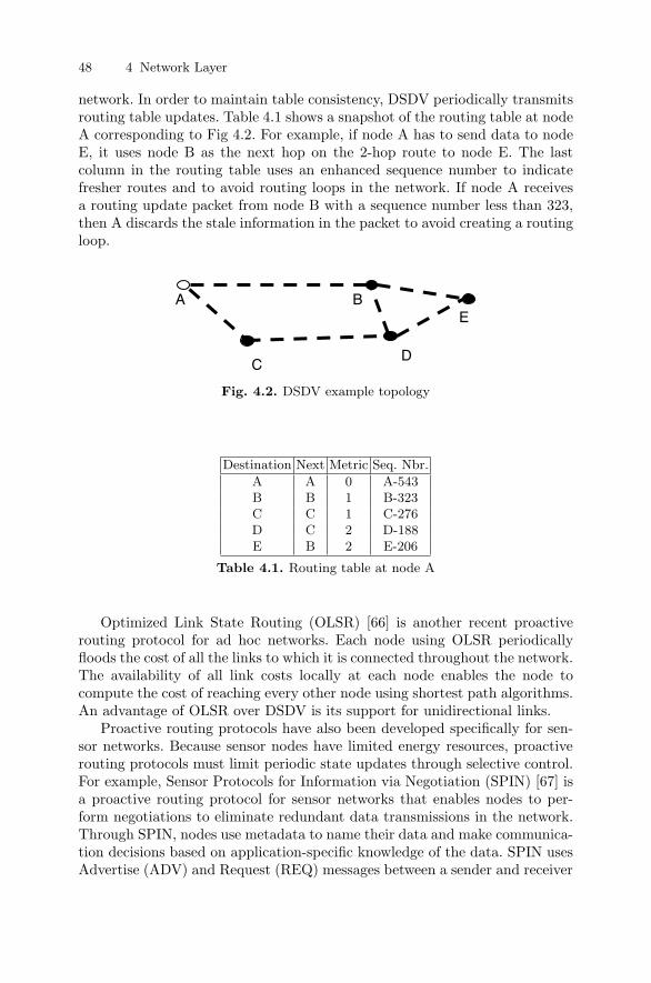
48 4 Network Layer
network. In order to maintain table consistency, DSDV periodically transmitsrouting table updates. Table 4.1 shows a snapshot of the routing table at nodeA corresponding to Fig 4.2. For example, if node A has to send data to nodeE, it uses node B as the next hop on the 2-hop route to node E. The lastcolumn in the routing table uses an enhanced sequence number to indicatefresher routes and to avoid routing loops in the network. If node A receivesa routing update packet from node B with a sequence number less than 323,then A discards the stale information in the packet to avoid creating a routingloop.
EA B
CD
Fig. 4.2. DSDV example topology
Destination Next Metric Seq. Nbr.
A A 0 A-543B B 1 B-323C C 1 C-276D C 2 D-188E B 2 E-206
Table 4.1. Routing table at node A
Optimized Link State Routing (OLSR) [66] is another recent proactiverouting protocol for ad hoc networks. Each node using OLSR periodicallyfloods the cost of all the links to which it is connected throughout the network.The availability of all link costs locally at each node enables the node tocompute the cost of reaching every other node using shortest path algorithms.An advantage of OLSR over DSDV is its support for unidirectional links.
Proactive routing protocols have also been developed specifically for sen-sor networks. Because sensor nodes have limited energy resources, proactiverouting protocols must limit periodic state updates through selective control.For example, Sensor Protocols for Information via Negotiation (SPIN) [67] isa proactive routing protocol for sensor networks that enables nodes to per-form negotiations to eliminate redundant data transmissions in the network.Through SPIN, nodes use metadata to name their data and make communica-tion decisions based on application-specific knowledge of the data. SPIN usesAdvertise (ADV) and Request (REQ) messages between a sender and receiver
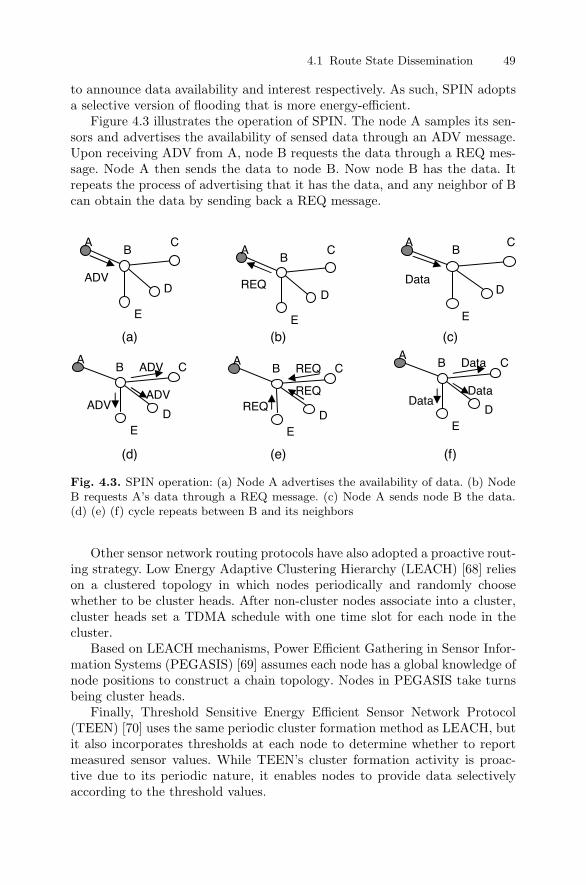
4.1 Route State Dissemination 49
to announce data availability and interest respectively. As such, SPIN adoptsa selective version of flooding that is more energy-efficient.
Figure 4.3 illustrates the operation of SPIN. The node A samples its sen-sors and advertises the availability of sensed data through an ADV message.Upon receiving ADV from A, node B requests the data through a REQ mes-sage. Node A then sends the data to node B. Now node B has the data. Itrepeats the process of advertising that it has the data, and any neighbor of Bcan obtain the data by sending back a REQ message.
REQ
REQREQ
ADV
AB
C
D
E
REQ
AB
C
D
E
Data
AB
C
D
E
AB C
DE
ADV
ADVADV
AB C
DE
AB C
DE
Data
DataData
(a) (b) (c)
(d) (e) (f)
Fig. 4.3. SPIN operation: (a) Node A advertises the availability of data. (b) NodeB requests A’s data through a REQ message. (c) Node A sends node B the data.(d) (e) (f) cycle repeats between B and its neighbors
Other sensor network routing protocols have also adopted a proactive rout-ing strategy. Low Energy Adaptive Clustering Hierarchy (LEACH) [68] relieson a clustered topology in which nodes periodically and randomly choosewhether to be cluster heads. After non-cluster nodes associate into a cluster,cluster heads set a TDMA schedule with one time slot for each node in thecluster.
Based on LEACH mechanisms, Power Efficient Gathering in Sensor Infor-mation Systems (PEGASIS) [69] assumes each node has a global knowledge ofnode positions to construct a chain topology. Nodes in PEGASIS take turnsbeing cluster heads.
Finally, Threshold Sensitive Energy Efficient Sensor Network Protocol(TEEN) [70] uses the same periodic cluster formation method as LEACH, butit also incorporates thresholds at each node to determine whether to reportmeasured sensor values. While TEEN’s cluster formation activity is proac-tive due to its periodic nature, it enables nodes to provide data selectivelyaccording to the threshold values.
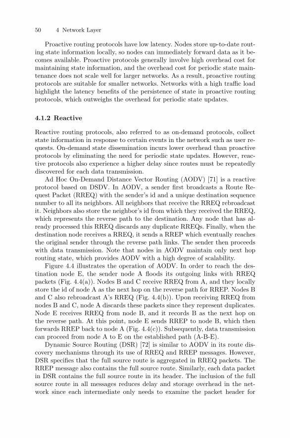
50 4 Network Layer
Proactive routing protocols have low latency. Nodes store up-to-date rout-ing state information locally, so nodes can immediately forward data as it be-comes available. Proactive protocols generally involve high overhead cost formaintaining state information, and the overhead cost for periodic state main-tenance does not scale well for larger networks. As a result, proactive routingprotocols are suitable for smaller networks. Networks with a high traffic loadhighlight the latency benefits of the persistence of state in proactive routingprotocols, which outweighs the overhead for periodic state updates.
4.1.2 Reactive
Reactive routing protocols, also referred to as on-demand protocols, collectstate information in response to certain events in the network such as user re-quests. On-demand state dissemination incurs lower overhead than proactiveprotocols by eliminating the need for periodic state updates. However, reac-tive protocols also experience a higher delay since routes must be repeatedlydiscovered for each data transmission.
Ad Hoc On-Demand Distance Vector Routing (AODV) [71] is a reactiveprotocol based on DSDV. In AODV, a sender first broadcasts a Route Re-quest Packet (RREQ) with the sender’s id and a unique destination sequencenumber to all its neighbors. All neighbors that receive the RREQ rebroadcastit. Neighbors also store the neighbor’s id from which they received the RREQ,which represents the reverse path to the destination. Any node that has al-ready processed this RREQ discards any duplicate RREQs. Finally, when thedestination node receives a RREQ, it sends a RREP which eventually reachesthe original sender through the reverse path links. The sender then proceedswith data transmission. Note that nodes in AODV maintain only next hoprouting state, which provides AODV with a high degree of scalability.
Figure 4.4 illustrates the operation of AODV. In order to reach the des-tination node E, the sender node A floods its outgoing links with RREQpackets (Fig. 4.4(a)). Nodes B and C receive RREQ from A, and they locallystore the id of node A as the next hop on the reverse path for RREP. Nodes Band C also rebroadcast A’s RREQ (Fig. 4.4(b)). Upon receiving RREQ fromnodes B and C, node A discards these packets since they represent duplicates.Node E receives RREQ from node B, and it records B as the next hop onthe reverse path. At this point, node E sends RREP to node B, which thenforwards RREP back to node A (Fig. 4.4(c)). Subsequently, data transmissioncan proceed from node A to E on the established path (A-B-E).
Dynamic Source Routing (DSR) [72] is similar to AODV in its route dis-covery mechanisms through its use of RREQ and RREP messages. However,DSR specifies that the full source route is aggregated in RREQ packets. TheRREP message also contains the full source route. Similarly, each data packetin DSR contains the full source route in its header. The inclusion of the fullsource route in all messages reduces delay and storage overhead in the net-work since each intermediate only needs to examine the packet header for
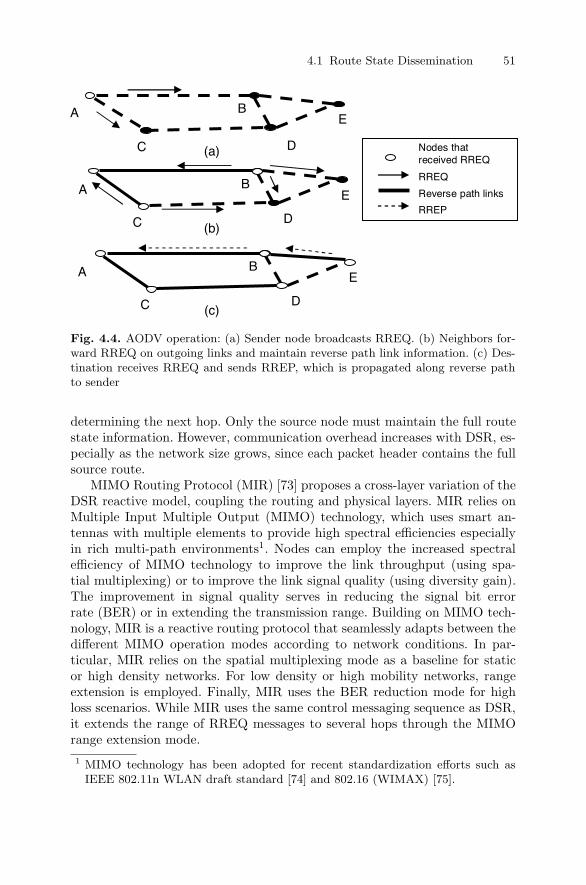
4.1 Route State Dissemination 51
A B
DC
E
A B
DC
E
A B
DC
E
Nodes that received RREQ
RREQ
Reverse path links
RREP
(a)
(b)
(c)
Fig. 4.4. AODV operation: (a) Sender node broadcasts RREQ. (b) Neighbors for-ward RREQ on outgoing links and maintain reverse path link information. (c) Des-tination receives RREQ and sends RREP, which is propagated along reverse pathto sender
determining the next hop. Only the source node must maintain the full routestate information. However, communication overhead increases with DSR, es-pecially as the network size grows, since each packet header contains the fullsource route.
MIMO Routing Protocol (MIR) [73] proposes a cross-layer variation of theDSR reactive model, coupling the routing and physical layers. MIR relies onMultiple Input Multiple Output (MIMO) technology, which uses smart an-tennas with multiple elements to provide high spectral efficiencies especiallyin rich multi-path environments1. Nodes can employ the increased spectralefficiency of MIMO technology to improve the link throughput (using spa-tial multiplexing) or to improve the link signal quality (using diversity gain).The improvement in signal quality serves in reducing the signal bit errorrate (BER) or in extending the transmission range. Building on MIMO tech-nology, MIR is a reactive routing protocol that seamlessly adapts between thedifferent MIMO operation modes according to network conditions. In par-ticular, MIR relies on the spatial multiplexing mode as a baseline for staticor high density networks. For low density or high mobility networks, rangeextension is employed. Finally, MIR uses the BER reduction mode for highloss scenarios. While MIR uses the same control messaging sequence as DSR,it extends the range of RREQ messages to several hops through the MIMOrange extension mode.1 MIMO technology has been adopted for recent standardization efforts such as
IEEE 802.11n WLAN draft standard [74] and 802.16 (WIMAX) [75].
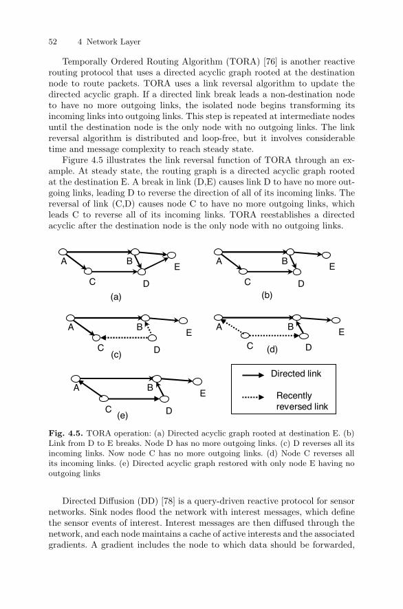
52 4 Network Layer
Temporally Ordered Routing Algorithm (TORA) [76] is another reactiverouting protocol that uses a directed acyclic graph rooted at the destinationnode to route packets. TORA uses a link reversal algorithm to update thedirected acyclic graph. If a directed link break leads a non-destination nodeto have no more outgoing links, the isolated node begins transforming itsincoming links into outgoing links. This step is repeated at intermediate nodesuntil the destination node is the only node with no outgoing links. The linkreversal algorithm is distributed and loop-free, but it involves considerabletime and message complexity to reach steady state.
Figure 4.5 illustrates the link reversal function of TORA through an ex-ample. At steady state, the routing graph is a directed acyclic graph rootedat the destination E. A break in link (D,E) causes link D to have no more out-going links, leading D to reverse the direction of all of its incoming links. Thereversal of link (C,D) causes node C to have no more outgoing links, whichleads C to reverse all of its incoming links. TORA reestablishes a directedacyclic after the destination node is the only node with no outgoing links.
Directed link
Recently reversed link
(a)
EA B
C D(d)
EB
C D
AE
B
C D(b)
A
EB
C D(c)
A
EB
C D(e)
A
Fig. 4.5. TORA operation: (a) Directed acyclic graph rooted at destination E. (b)Link from D to E breaks. Node D has no more outgoing links. (c) D reverses all itsincoming links. Now node C has no more outgoing links. (d) Node C reverses allits incoming links. (e) Directed acyclic graph restored with only node E having nooutgoing links
Directed Diffusion (DD) [78] is a query-driven reactive protocol for sensornetworks. Sink nodes flood the network with interest messages, which definethe sensor events of interest. Interest messages are then diffused through thenetwork, and each node maintains a cache of active interests and the associatedgradients. A gradient includes the node to which data should be forwarded,
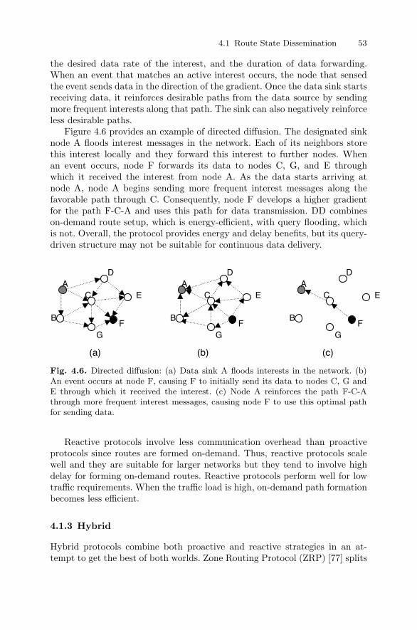
4.1 Route State Dissemination 53
the desired data rate of the interest, and the duration of data forwarding.When an event that matches an active interest occurs, the node that sensedthe event sends data in the direction of the gradient. Once the data sink startsreceiving data, it reinforces desirable paths from the data source by sendingmore frequent interests along that path. The sink can also negatively reinforceless desirable paths.
Figure 4.6 provides an example of directed diffusion. The designated sinknode A floods interest messages in the network. Each of its neighbors storethis interest locally and they forward this interest to further nodes. Whenan event occurs, node F forwards its data to nodes C, G, and E throughwhich it received the interest from node A. As the data starts arriving atnode A, node A begins sending more frequent interest messages along thefavorable path through C. Consequently, node F develops a higher gradientfor the path F-C-A and uses this path for data transmission. DD combineson-demand route setup, which is energy-efficient, with query flooding, whichis not. Overall, the protocol provides energy and delay benefits, but its query-driven structure may not be suitable for continuous data delivery.
D
E
(a) (b) (c)
FG
B
AC
D
E
FG
CA
B
D
E
FG
C
B
A
Fig. 4.6. Directed diffusion: (a) Data sink A floods interests in the network. (b)An event occurs at node F, causing F to initially send its data to nodes C, G andE through which it received the interest. (c) Node A reinforces the path F-C-Athrough more frequent interest messages, causing node F to use this optimal pathfor sending data.
Reactive protocols involve less communication overhead than proactiveprotocols since routes are formed on-demand. Thus, reactive protocols scalewell and they are suitable for larger networks but they tend to involve highdelay for forming on-demand routes. Reactive protocols perform well for lowtraffic requirements. When the traffic load is high, on-demand path formationbecomes less efficient.
4.1.3 Hybrid
Hybrid protocols combine both proactive and reactive strategies in an at-tempt to get the best of both worlds. Zone Routing Protocol (ZRP) [77] splits
54 4 Network Layer
the network into zones. For intrazone communications, ZRP uses proactiverouting. For interzone communication, it uses reactive routing.
Rumor Routing (RR) [79] is a hybrid protocol that is similar to DirectedDiffusion. RR attempts to balance event and query flooding in sensor net-works. Whenever an event happens, a node employs an agent, which is along-lived packet, to traverse the network and notify distant nodes of theevent. In essence, the event-based creation of agents in RR is the protocol’sreactive aspect. The proactive aspect is the agent traversal of the network,which notifies random - occasionally uninterested - nodes of the occurrenceof an event. RR reduces the overhead of query flooding and it performs wellin networks with infrequent events. The drawback of RR is the high overheadfor maintaining agent and event tables.
Although hybrid protocols could theoretically integrate favorable featuresof both proactive and reactive protocols, research on hybrid protocols has sofar been limited. The main idea of hybrid protocols is achieving a balancebetween the energy-efficiency of on-demand route setup and the rapid datatransmission in proactive routing. A key challenge for hybrid protocols isdetermining this optimal balance and providing flexible means for tuning theprotocol for different applications.
4.2 Topology
In this section, we discuss the effect of topology on the performance of arouting protocol for ad hoc and sensor networks. Within this context, topologyemerges here as a cross-layer aspect, since it impacts the routing behavior,as well as the MAC behavior. We examine routing protocols in light of thefour topology categories we introduced in Section 3.4. We further identify andpresent the multi-hierarchy topology in our discussion for routing protocols.
4.2.1 Single Hop and Centralized Topologies
Routing is straightforward in both single hop and centralized topologies. In asingle hop topology, each node can broadcast its packet to all neighbors. Theintended receiver hears the packet and processes it. All other nodes discardthe packet after examining the destination address.
In a centralized topology, the central base station is within range of allnodes. When the base station receives a transmitted packet, it simply deter-mines where it needs to forward the packet in order to reach the intendedreceiver. The next hop could be either the destination itself, or an intermedi-ate node. In either case, all nodes other than the base station are not involvedin routing decisions.
Although single hop and flat topology networks involve simple routingmechanisms, they lack the scalability for supporting large scale ad hoc andsensor networks.
4.2 Topology 55
4.2.2 Multiple Hop Flat Topology
A multiple hop flat topology assumes all nodes are homogeneous in resourcesand that network traffic is random. In most cases, a multiple hop flat topologycan help promote fairness and load balancing in the network.
Many general purpose ad hoc network routing protocols adopt a multihopflat topology [66, 71, 72, 76, 182]. Flexibility is a primary benefit of using thistopology. Because the protocols view all nodes equally, multiple hop flat topol-ogy protocols can easily handle a failure or congestion at a particular nodeby rerouting data along new paths, provided there is sufficient node densityto do so.
Some sensor network-specific routing protocols also adopt a multiple hopflat topology. For example, SPIN adopts a multiple hop flat topology whichassumes that all the nodes are possible data sinks. All the nodes in SPIN arealso capable of acting as sources by issuing ADV messages. Another sensornetwork routing protocol that adopts this topology is Minimum Cost Forward-ing (MCF) [80]. MCF enables nodes to independently compute their routingcost from a data sink. Discovery of routing cost occurs progressively by sum-ming up the cost of the immediate link with the next hop and the reportedcost of the next hop to the sink.
In larger networks with a multihop flat topology, the hop count to certaindestinations and the routing state stored at each node could become too largefor the routing protocol to handle. Furthermore, as the average number ofroute hops increases in a network, so does the potential for transmission errorsand retransmissions. These shortcomings of multihop flat topology networkshave led to the design of protocols with a clustered topology to support largescale networks.
4.2.3 Clustered Topology
In a clustered topology, a subset of the nodes act as leaders or cluster heads.All the other nodes associate themselves with at least one cluster head. Anode associated with a particular cluster head i is said to belong to cluster i.The cluster head acts as a virtual base station for the nodes within its cluster.Cluster head functionality may include forwarding the data of nodes withinits cluster, managing its cluster’s topology, and scheduling the transmission ofnodes. A clustered topology reduces the energy consumption of most nodes byshifting most of the network management burden to the cluster head. Clusterhead selection may be either static or dynamic. Topologies with a static orfixed cluster head are less fault tolerant because the cluster head represents asingle point of failure for the nodes in the cluster.
Routing protocols that enable dynamic selection of the cluster head elim-inate the single point of failure issue, but they involve more communicationdelay and control overhead for the repeated election of the cluster head. Clus-ter head Gateway Switch Routing (CGSR) [81] is a proactive clustered routing
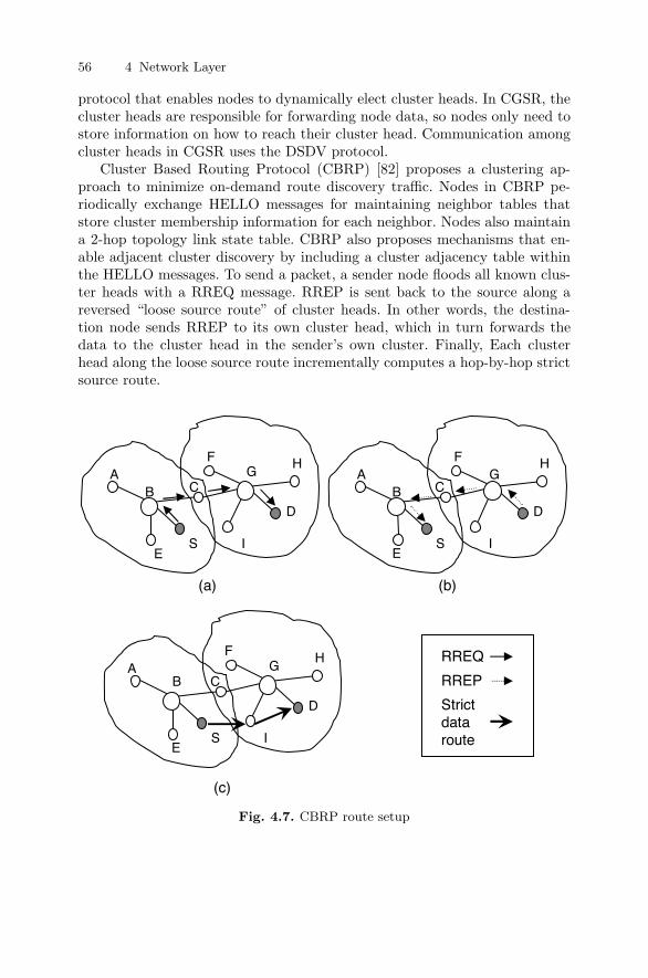
56 4 Network Layer
protocol that enables nodes to dynamically elect cluster heads. In CGSR, thecluster heads are responsible for forwarding node data, so nodes only need tostore information on how to reach their cluster head. Communication amongcluster heads in CGSR uses the DSDV protocol.
Cluster Based Routing Protocol (CBRP) [82] proposes a clustering ap-proach to minimize on-demand route discovery traffic. Nodes in CBRP pe-riodically exchange HELLO messages for maintaining neighbor tables thatstore cluster membership information for each neighbor. Nodes also maintaina 2-hop topology link state table. CBRP also proposes mechanisms that en-able adjacent cluster discovery by including a cluster adjacency table withinthe HELLO messages. To send a packet, a sender node floods all known clus-ter heads with a RREQ message. RREP is sent back to the source along areversed “loose source route” of cluster heads. In other words, the destina-tion node sends RREP to its own cluster head, which in turn forwards thedata to the cluster head in the sender’s own cluster. Finally, Each clusterhead along the loose source route incrementally computes a hop-by-hop strictsource route.
D
S
AF
E
GH
I
D
S
AF
C
E
GH
I
D
S
AF
B C
E
GH
I
(a) (b)
(c)
RREQ
RREP
Strict data route
B BC
Fig. 4.7. CBRP route setup
4.2 Topology 57
Figure 4.7 illustrates the route setup process in CBRP. The sender nodeS wants to send data to the destination D. To find a route to node D, node Sfloods the accessible cluster heads B and G with RREQ messages (Fig. 4.7(a)).Node G determines that the RREQ is meant for a node within its cluster, soit forwards the RREQ to node D. In response, node D sends a RREP messageto its cluster head node G, which forwards the RREP on the reverse route ofRREQ back to S (Fig. 4.7(b)). The reverse path is a loose source route since ittraverses the cluster heads and doesn’t necessarily represent the shortest routebetween S and D. Upon receiving RREP, the cluster heads G and B computethe strict source route through which data will flow from S to D (Fig. 4.7(c)).
A class of sensor network routing protocols, including LEACH, PEGASIS,and TEEN, also use a dynamic cluster topology. The goal in all three protocolsis to balance energy consumption among the sensor nodes, which are assumedto be homogeneous, by rotating the role of cluster head. LEACH segmentstime into rounds, where the initial setup phase of each round handle thecluster setup for the round. Nodes use a local algorithm to decide whetherto be cluster heads for this round, and non-cluster nodes associate with oneof the neighboring cluster heads. PEGASIS relies on geographic informationthat is locally available at each node in order to rotate the role of cluster fairlyamong the nodes.
Clustered topologies introduce a hierarchy into the network topology byfocusing the routing at a few designated nodes. Generalizing the hierarchicalmodel leads us to the topic of the next section: routing in multilevel hierar-chical networks.
4.2.4 Multilevel Hierarchical Networks
Multilevel hierarchical (MLH) topology networks represent a superclass ofclustered networks. Instead of designating nodes as simply cluster heads ordata nodes, multilevel hierarchical protocols enable several hierarchical levels,forming a logical tree routing structure. Cluster heads at one level can formclusters of their own and select a higher level cluster head. MLH protocolsprovide more scalability over other topology types. A comprehensive surveyof MLH routing protocols is available in [92].
Adaptive Routing using Cluster Hierarchies (ARCH) [93] is a MLH pro-tocol that enables neighboring mobile nodes to exchange periodic HELLOmessages for adapting the number of levels in the hierarchy to the networksize. If the network size increases, nodes will form an additional hierarchicallevel and vice versa. ARCH provides route robustness by ensuring that noncluster head nodes are connected to more than one cluster head, so that if acluster head becomes unavailable, a node uses the alternative cluster head.
Hierarchical State Routing (HSR) [83] is another MLH protocol that dis-tinguishes between the physical routing hierarchy, which is dictated by geo-graphic locations of nodes, and the logical topology of the network, determined
58 4 Network Layer
by logical node groups. HSR borrows concepts from the Mobile Internet Pro-tocol [84], such as home agents and tunneling, to implement a group mobilitymodel that is applicable for application scenarios in which nodes move as agroup, such as battle conditions or disaster recovery. The logical partitionsand mobility model reduce the update overhead in highly mobile situations.The drawbacks of HSR are the possibility for non-optimal routing, which isincurred by tunneling, and the increased complexity.
In sum, MLH protocols adopt the most scalable and general topology.Large scale networks can exploit MLH topologies effectively, but small ormedium scale network applications should consider the added complexity anddelay of maintaining a multilevel hierarchical topology.
4.3 Multipath Routing
The traditional routing approach is to forward packets along the best sin-gle route from a source to destination. Although this approach is simple andstraightforward, it suffers from poor fault tolerance. Any break in the singleroute from source to destination requires the determination and establishmentof another suitable route. Route reestablishment involves increased communi-cation overhead and delay. In addition, applications that require continuousdata transmissions may not tolerate interruptions during route reestablish-ment.
More recent research has explored establishing multiple paths betweena source and destination, which gives rise to the term “multipath routing”.Multipath routing not only reduces the fault tolerance of a routing protocol,but it also provides better load balancing in the network. Nodes can spreadthe traffic more evenly among several paths to avoid the creation of hot spotsin the network. Finally, multipath routing also enables higher bandwidth fortraffic streams by aggregating the bandwidth capability of several paths. Ofcourse, multipath routing also has drawbacks such as increased complexityand overhead. Nodes have to store more state and exchange more controlmessages for maintaining multiple paths.
For example, Chen et al. [105] propose multiple disjoint paths with oneprimary path and multiple secondary routes which are maintained throughperiodic control signalling. Chen et al.’s protocol routes most of the packetsalong the primary path, and it uses the secondary paths when the primarypath becomes congested or unavailable. The work in [105] uses end-to-enderror control in which the final destination can notify the sender of errorsalong the path.
Similar multipath routing protocols [36, 106] propose using partially dis-joint paths instead. Reference [106] proposes per-hop rather than end-to-endacknowledgements, to better adapt to the dynamic network environment andto detect fault more quickly.
4.4 Power-awareness 59
Meshed MultiPath Routing [108] departs from the concept of primaryroutes and it enables equal use of the established routes. The rationale be-hind the equal use of routes is to promote load balancing and to avoid theexhaustion of node resources along the primary routes.
In sum, multipath routing is promising for large networks because it en-sures transmission continuity and fault tolerance. Establishing and storing thestate for multiple paths may be too costly, so gradient-based protocols, suchas directed diffusion, may be a better option for multipath routing.
4.4 Power-awareness
The small form factor and mobility of nodes in ad hoc and sensor networksimpose the use of small and portable batteries with limited energy resources.Because the nodes function as routers in addition to their data transmissionfunction, energy efficient mechanisms are critical in ad hoc and sensor net-works. As a result, many proposed routing protocols attempt to incorporateenergy considerations from across the communication stack into routing deci-sions, representing another cross-layer optimization. The discussion in Chap-ters 7 through 9 further elaborates on using power-related information forcross-layer optimizations.
Minimum Total Transmission Power Routing (MTPR) [94] is a power-aware routing protocol for ad hoc networks. MTPR is an on-demand protocolthat assigns link costs proportionally to the transmission power required tomaintain an acceptable Signal to Noise Ratio (SNR) for the link. Nodes thenselect the minimum energy path through a shortest path algorithm based onlink costs. However, the resulting path in MTPR is not necessarily the pathwith the minimum number of hops, which may result in higher delays andmore power consumption at intermediate nodes. In an attempt to overcomethis drawback of MTPR, Minimum Total Transceiving Power (MTTP) [95]adopts a link cost metric that includes both the transmission power as wellas receiving power.
While protocols based on transceiver power reduce power consumption inthe network, these protocols do not ensure a longer network lifetime. To thisend, researchers have proposed protocols that incorporate the battery energyof nodes into routing decisions. For instance, Minimum Battery Cost Rout-ing (MBCR) [96] provides a battery cost function that is inversely proportionalto the remaining battery capacity at each node. The cost of a path in MBCRis the sum of costs of nodes along the path. When all nodes have comparableresidual battery capacity, nodes using MBCR select shortest hop routes. Oth-erwise, they select minimum energy routes. The drawback of MBCR is thatit may overuse intermediate nodes because the path cost only minimizes theaggregated cost instead of individual node battery costs.
Toh proposes Conditional Max-Min BCR (CMMBCR) [186] which com-bines power considerations for both the transmission power on links and bat-
60 4 Network Layer
tery capacity of nodes. CMMBCR uses battery capacity instead of a batterycost function as a routing metric. Routing decisions in CMMBCR only con-sider paths with nodes that have sufficient remaining battery capacity. Amongthe eligible paths, CMMBCR chooses the path with the minimum transmis-sion power.
Shah and Rabaey [187] introduce network survivability as an improvedrouting metric, particularly for sensor networks. In other words, their con-tention is that a protocol should maintain connectivity in a network for thelongest duration possible. Unlike previous protocols, they propose storing sev-eral suboptimal paths at each sender in addition to the optimal path. The basisfor this proposal is that always using the lowest energy path is not beneficialfor the long-term energy health of a sensor network. The transmission can thenuse the multiple paths through a probabilistic scheme in order to balance en-ergy consumptions across the multiple paths and to ensure that nodes close todata sinks do not deplete their resources early. This protocol adopts a routingmetric combining link transmission power and residual battery capacity atnodes.
Jurdak [100] proposes a cross-layer routing cost metric for sensor networksbased on the radio, processor, and sensor activity. In Jurdak’s approach, anode compares the power consumption of a neighbor relative to the averagepower consumption of its other neighbors through a weighted sum of dutycycles of the all components of a sensor node. This routing metric replaces theremaining battery capacity with the radio duty cycle because battery voltagereadings in sensor nodes are unreliable [101] and their fluctuations may leadto inefficient or oscillating routes. Chapter 10 provides further details on thismetric.
Another perspective that implicity minimizes radio power consumption isto minimize the expected total number of packet transmissions (including re-transmissions) for delivering packets to their final destination, as proposed byDe Couto et al. [99]. Their strategy highlights the energy inefficiency of mini-mum hop count routing in the presence of lossy wireless links. Minimum hoproutes typically maximize the distance traveled at each hop, which reducessignal strength and maximizes the loss ratio of data packets and the corre-sponding acknowledgement packets, causing many retransmissions. Anotherdrawback of traditional routing metrics is their lack of consideration of linkasymmetries, such as unidirectional links. To address these issues, De Coutoet al. propose the expected transmission count (ETX) routing metric, whichis inversely proportional to the product of the forward and reverse packet de-livery ratios. By considering both forward and reverse packet delivery ratios,ETX addresses the asymmetric link issue. The dependence of routes on deliv-ery ratios also improves throughput and minimizes spectrum use. In practicalterms, nodes that employ the ETX routing metric snoop on the neighborhoodlinks to keep track of the forward and reverse delivery ratio on each link. TheETX routing metric is by definition a cross-layer routing metric, as it employslink layer information for determining behavior at the routing layer.
4.5 Geographical Routing 61
4.5 Geographical Routing
Geographic routing protocols assume that location information is availableat the nodes through GPS or similar localization systems. Nodes can exploitavailable location information to route data in the geographic direction of thedestination, yielding a more efficient routing strategy.
The main challenge of geographic routing protocols is the implementationand resource cost for providing location information. For example, having aGPS receiver provides each node with absolute location coordinates. However,providing nodes with location information is not without cost – to equip allnodes with GPS receivers incurs considerable monetary cost and causes higherenergy consumption at the nodes. More efficient techniques for localizationinclude signal strength [85] or time-of-flight measurements [86] along withlocal triangulation to provide nodes with relative location information. Hybridlocalization methods combine the absolute positioning capability of GPS withaffordable and energy-efficient localization techniques. For example, a networkcould include a few nodes with GPS receivers which provide absolute locationinformation and act as location servers. Other nodes compute their locationrelative to the GPS-equipped nodes in order to eventually infer their ownabsolute location information.
Beyond the issue of collecting location information, geographic routingprotocols exploit available location information through different strategies.Greedy Perimeter Stateless Routing (GPSR) [87] uses location informationto forward packets to nodes in the general direction of the final destination.Whenever a greedy path does not exist (i.e., the only path which requires dataforwarding to move temporarily farther away from the destination), GPSRrecovers by forwarding in perimeter mode, in which a packet traverses succes-sively closer faces of a planar subgraph of the full radio network connectivitygraph. This process repeats until a node closer to the destination is reached,at which point greedy forwarding resumes.
Location-aided Routing (LAR) [88] is another proposed geographical rout-ing protocol that uses location information to limit the search space for a de-sired route. LAR defines the concepts of expected zone and request zone. Theexpected zone is the estimated region of the destination’s current location,based on the most recent update of the destination’s position and speed. Toset up an on-demand route, the sender can limit route request messages to theexpected region. While the expected region estimates the location of the finaldestination, the concept of request region specifies the region within whichan intermediate node forwards the route requests. By limiting the forwardingof route requests, LAR yields significant reductions in control overhead overflooding.
Grid Location Service (GLS) [89] is another geographic routing protocolthat aims to provide the following features: load balancing; fault tolerance;local collaboration; and limited storage overhead. GLS employs the concept oflocation servers that store location information. Each node acts as a location
62 4 Network Layer
server on behalf of some other nodes. The selection of location servers avoidselection techniques. Instead, each node probabilistically determines a subsetof nodes to act as its location servers in order to spread the load evenly amongnodes. The location servers of a node are dense in regions close to the node,and they become more sparse as we move further away from the node. Nodescan query the location servers of the intended destination to determine thecurrent location of the destination.
Seada et al. [90] propose new strategies for geographic routing under therealistic conditions of lossy wireless links in sensor networks. Their contentionis that traditional geographic routing protocols employ a maximum distancegreedy forwarding technique, without regard to the variance of quality inlonger distance links. With a rationale similar to that of ETX, Seada et al.’sultimate goal is the maximization of the number of packets delivered to thesink for each unit of energy spent in a geographic routing network. In fact,the collection of link variables is identical to the technique of De Couto etal. [99]. Seada et al. also investigate cross-layer routing metrics that rely onlink layer information, most notably the PRR metric [91] that incorporatesinformation on a link’s SNR, encoding ratio, and frame length. For more se-lective geographic forwarding, they propose several techniques for blacklistingneighboring links in the route decision process, based on combinations of dis-tance and reception rate considerations. Based on analysis, simulations andtest-bed studies, they conclude that the most expressive routing metric forgeographic forwarding is the product of PRR and distance.
In sum, geographical routing trades off reduced control overhead and re-duced delay in forwarding data with the increased energy and communicationoverhead for collection and maintenance of accurate location information. Theimplementation of geographical routing through a hierarchical or clusteredtopology can limit routing state storage at each cluster or level, providinga high degree of scalability. Greedy geographic forwarding decisions shouldconsider the energy-distance trade-off to maximize throughput and minimizepacket losses in lossy wireless environments that are characteristic of ad hocand sensor networks.
4.6 Quality-of-Service
Energy-efficient operation is a key goal for many applications in ad hoc andsensor networks, but there are also other quality of service metrics that maybe even more important for particular applications. For example, an ad hocnetwork for disaster relief requires minimum delay in the network in orderto maximize chances for finding survivors. In another application, a sensornetwork for detecting toxic leaks in a factory may prioritize high reliabilityover all other considerations. As a result, routing techniques for ad hoc andsensor networks have been developed for supporting more general QoS guar-antees. Enforcing QoS policies usually benefits from cross-layer design since
4.6 Quality-of-Service 63
it may require access to information from higher layers, such as applicationmeta data, and from lower layers, such as acknowledgements from the logicallink control layer.
QoS-based routing protocols aim at satisfying one or more performancegoals at the network or node level. Performance goals include robustness, lowdelay, high reliability, energy efficiency, and high throughput.
Protocols for general purpose ad hoc networks should provide QoS on thenode level. Nodes in ad hoc networks operate as independent entities, andthey have individual communication goals. Therefore, the QoS guarantees inad hoc networks must enable per node and even per connection performanceoptimization.
Core Extraction Distributed Ad hoc Routing (CEDAR) [198] is a QoSrouting algorithm with a primary goal to provide robustness. CEDAR firstextracts a subset of nodes, the so-called core, through local computations tomaintain network routing state. The core nodes propagate link state infor-mation to remote nodes in the network. In particular, core nodes report thestable high bandwidth links and the unfavorable links to remote nodes, whichcan then use this information for routing decisions. Non-core nodes only needto determine their routing path to the appropriate core node. Core nodes thenforward the packets in the direction of the destination.
Baldi et al. [175] propose a generalized cost function for supporting admis-sion control in wireless ad hoc networks that use Ultra Wide Band (UWB)radio. Their cost function is a weighted sum of several link cost metrics: trans-mission power; link setup; interference; quality; and delay. The weights of in-dividual cost metrics can be customized according to different applicationsand hardware. For instance, a delay-sensitive application might assign a highweight for the delay cost metric. The cost function also enables the inclusionof additional cost metrics as needed. Admissible links or paths must satisfycost constraints in the network. Although originally designed for UWB net-works, this cost function can be adapted to more general ad hoc networks andcan be integrated as the cost metric of many cost-based routing protocols.
Unlike most general purpose ad hoc networks, providing QoS guarantees insensor networks must consider network-wide performance goals, since sensornetworks typically have a single operator or user. For example, prolongingthe lifetime of the network as a whole is more important than optimizing thelifetime of a single node in a sensor network.
Sequential Assignment Routing (SAR) [103] is a QoS routing protocol forsensor networks. SAR assumes that the sensor network has a single data sink.Rather than generating a single path to the sink, the protocol enables eachnode to generate multiple paths to avoid route recomputation overhead when-ever a route fails. SAR builds multiple trees, with each tree rooted at a one-hopneighbor of the sink, in order to provide multiple paths to the sink. The pro-tocol also adopts a general QoS metric representation. Each data node canchoose its path to the data sink based on its stored information regarding the
64 4 Network Layer
energy resources and the cumulative quality-of-service parameters associatedwith each path towards the sink.
Energy Aware QoS Routing [104] is a protocol for sensor networks thataims at providing bandwidth and delay guarantees in an energy-efficientmanner. The protocol addresses networks with both real-time and non real-time traffic. It attempts to minimize end-to-end delay for real-time trafficwhile maximizing throughput for non real-time traffic. The protocol computescost for links independently, except for end-to-end delay which is aggregatedfor links along a path. The protocol’s cost function incorporates transceiverpower, sensing power, residual battery energy, energy consumption rate, anderror rate. It also includes a metric that quantifies the cost of switching anode from inactive to forwarding state, and another metric that penalizesnodes with a large forwarding load.
In sum, reliability, delay, robustness, and throughput are important per-formance considerations for ad hoc and sensor networks. Routing protocolsthat support QoS enforcement tend to provide tunable mechanisms that en-able network designers to determine the relevant QoS parameters and theirrelative importance.
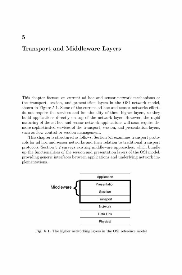
5
Transport and Middleware Layers
This chapter focuses on current ad hoc and sensor network mechanisms atthe transport, session, and presentation layers in the OSI network model,shown in Figure 5.1. Some of the current ad hoc and sensor networks effortsdo not require the services and functionality of these higher layers, so theybuild applications directly on top of the network layer. However, the rapidmaturing of the ad hoc and sensor network applications will soon require themore sophisticated services of the transport, session, and presentation layers,such as flow control or session management.
This chapter is structured as follows. Section 5.1 examines transport proto-cols for ad hoc and sensor networks and their relation to traditional transportprotocols. Section 5.2 surveys existing middleware approaches, which bundleup the functionalities of the session and presentation layers of the OSI model,providing generic interfaces between applications and underlying network im-plementations.
Application
Presentation
Session
Transport
Network
Data Link
Physical
{Middleware
Fig. 5.1. The higher networking layers in the OSI reference model
66 5 Transport and Middleware Layers
5.1 Transport Layer
The transport layer is responsible for flow control, congestion control, end-to-end connection setup, and end-to-end reliability. The most popular trans-port protocols for Internet applications are Transmission Control Proto-col (TCP) [109] and the User Datagram Protocol (UDP) [110]. TCP is areliable byte-stream connection-oriented protocol, while UDP is a best-effortconnectionless protocol. Both TCP and UDP were originally designed forwired networks long before the conception of ad hoc networks. As such, theseprotocols do perform well in the highly dynamic wireless environment of adhoc and sensor network applications. This has led to several enhancementsover the traditional protocols and to the proposal of new transport protocolsfor ad hoc and sensor networks, which we discuss in this section.
The remainder of this section is organized as follows. Section 5.1.1 pro-vides a brief description of the traditional transport protocols and why theyare incompatible with ad hoc and sensor networks. The remaining two subsec-tions present transport protocols specifically designed for ad hoc and sensornetworks, most of which protocols integrate cross-layer optimizations. Sec-tion 5.1.2 discusses the general-purpose transport protocols for ad hoc net-works that focus on preserving session connectivity and information flow inhighly dynamic environments. Section 5.1.3 explores novel sensor networktransport protocols, which tend to exploit application specific information forimproving performance.
5.1.1 TCP and UDP
UDP provides a transaction-oriented datagram service above the IP layerwithout providing any guarantees of delivering or maintaining the order ofpackets. The main contribution of UDP is to support several concurrent ap-plications over the same IP interface through the introduction of ports thatare bound to the applications.
The most widely used transport protocol, TCP, currently accounts formore than 90% of Internet traffic. TCP’s design goals include:
1. Reliability: TCP provides reliable end-to-end data delivery through ACKmessages.
2. Congestion control: TCP attempts to limit excess traffic in the networkin order to maintain acceptable transfer rates.
3. Flow control: a process by which a receiver adapts the per-flow trafficto its reception capacity.
In order to perform both congestion control and flow control, TCP uses anelastic congestion window. The size of the congestion window is adjusted ac-cording to the traffic requirements in the network.
The basic algorithm in TCP works as follows. The TCP sender initiallysets the congestion window size to 1 packet, proceeds to send its first data
5.1 Transport Layer 67
packet, and sets a local timer. If the sender receives an ACK message beforethe timer expires, then the sender doubles the congestion window to 2 packets,sends the next 2 data packets to the destination and sets a new timer. Aslong is all the ACK messages are received in time, the sender doubles thewindow again. This process is referred to as “slow-start” of TCP. The TCPreceiver also includes in its ACK messages the current buffer capacity at thereceiver, referred to as the receiver window. The slow-start phase continuesuntil the window size reaches a preset slow-start threshold, at which point thesender begins increasing the window size by 1 packet upon the reception ofevery successful ACK. This phase is called congestion avoidance, as it tries toanticipate that the exponential growth in window size during the slow startphase will surely cause congestion. Congestion avoidance persists until thesender’s window size reaches the receiver window size and remains constantafter that. Whenever an ACK message does not arrive in time at the TCPsender, the sender assumes that the packet loss is due to congestion and itinvoke TCP’s congestion control mechanisms. Subsequently, the sender resetsits congestion window to 1 packet, resets its slow-start phase, and halvesthe slow-start threshold. The sender then proceeds in doubling the congestionwindow at every successful ACK and the process continues as described above.
The congestion control mechanism in classic TCP causes oscillations inthe congestion window since every lost or duplicate ACK drops the congestionwindow back to 1 packet and resets the slow-start phase. Several extensionshave been proposed [111–113] for improving the performance of TCP overtraditional wired networks. One prominent extension is TCP Reno [111] inwhich the congestion window is set to half of its current value upon a failureto receive ACK or upon reception of a duplicate ACK. Upon reception ofadditional duplicate ACK messages, TCP Reno increments the congestionwindow linearly at 1 packet per duplicate ACK reception.
Because their design targets traditional networks, the congestion control,flow control, and end-to-end acknowledgement mechanisms yield poor per-formance when TCP is deployed in an ad hoc or sensor network. To be-gin with, the TCP congestion control mechanism always assumes that a lostACK packet results from network congestion. In ad hoc and sensor networks,the distributed nature of the network leads to more frequently missed ACKsdue to MAC layer issues (such as collisions, hidden terminal problems, andco-channel interference) and routing issues (such as node mobility or disap-pearance, intermittent or unidirectional wireless links, and path breaks). Thehigh possibility of missed ACKs causes the TCP congestion window to dropback to 1 packet more frequently, yielding low throughput and low channelutilization.
MAC layer issues can cause degraded performance for TCP over ad hocand sensor networks. Collisions and hidden terminal problems are more likelyin ad hoc and sensor network links because of the distributed channel accessmechanisms. Furthermore, the broadcast nature of the wireless channel causesinterference among coexisting transmissions. These MAC layer issues lead
68 5 Transport and Middleware Layers
individual links to suffer higher packet losses along a TCP path, resulting ina higher number of missed ACK packets at the receiver.
Routing issues also contribute to the degradation of the congestion windowmechanism of TCP over ad hoc and sensor networks. Because of the dynamictopology and node mobility, ad hoc and sensor network routes are longer andless stable than traditional networks, which leads to more frequent lost ACKs.Also, unidirectional links cause ACK losses since the end-to-end reliabilitymechanism in TCP assumes bidirectional links. Finally, the multi-path routingprotocols in Section 4.3 that distribute data delivery over multiple routesmay cause packets to arrive out-of-order at the receiver. Out-of-order packetscause the receiver to issue duplicate ACKs, leading the sender to invoke thecongestion control mechanism.
5.1.2 Ad Hoc Network Transport Protocols
To overcome the drawbacks of traditional transport protocols, researchershave proposed several transport protocols that are customized for ad hocnetworks. Some of the proposed protocols are modifications of the originalTCP, while others are completely new protocols.
TCP Enhancements
The dependence of TCP performance on lower layer attributes has led to thedesign of TCP-based enhancements that exploit cross-layer information forbetter operation over ad hoc and sensor networks. All of these enhancementsaddress the high probability of packet losses due to the unreliability of in-dividual links and routes. In particular, the common direction is to providemechanisms to notify the sender of the cause of packet losses and to freezethe congestion window algorithm while the problem is rectified.
One of the enhancements for ad hoc and sensor networks is TCP withexplicit link failure notification (TCP-ELFN) [114]. TCP-ELFN enables anintermediate node to detect a link failure along an active path and it noti-fies the TCP sender through control messages to freeze the retransmissiontimers and the congestion window. The TCP sender then uses periodic probepackets to determine when the receiver is reachable, at which point it restartsthe timers and data transmission. Because TCP-ELFN relies on link failurenotification, it has little dependence on routing layer functionality. One draw-back of TCP-ELFN is that a new route to the receiver may not support thecongestion window of the old broken route.
Other enhancements use similar feedback mechanisms [115–117], but theseenhancements notify the sender of a break in the path rather than an explicitspecification of which link has failed. Feedback based TCP (TCP-F) [115] en-ables the node that detects a path break to notify the sender through routinglayer control messages. Upon notification of a path break, the sender entersinto snooze state, freezing the data transmission, congestion window size, and
5.1 Transport Layer 69
all timers until a path to the destination can be reestablished. The node thatdetects the path break also propagates this knowledge to other nodes. Anyintermediate node on the original path that has an alternate route to the des-tination can notify the sender of this route, at which point data transmissionresumes. The advantage of TCP-F lies in its simplicity and effectiveness. Oneof its drawbacks is the requirement for network layer support for path breaknotification. Another drawback is that the new snooze state for TCP-F re-quires modifications with original TCP state machine, which makes TCP-F aless attractive option for widespread adoption.
To remedy this issue, Ad Hoc TCP (ATCP) [117] uses a similar feedbackmechanism to TCP-F without creating a new state in the TCP state machine.Instead, it introduces a new ATCP layer between the transport and networklayer. ATCP distinguishes between three causes of packet loss: network parti-tion; transmission errors; and congestion. In the case of a network partition,ATCP puts the sender in persist mode so that it doesn’t needlessly retrans-mit packets. For transmission errors, the sender retransmits packets withoutinvoking the congestion control. Finally, in case of congestion, ATCP invokesthe congestion control mechanism at the sender. Because ATCP mechanismswork at a separate layer that is transparent to the transport layer, ATCP en-ables full compatibility with traditional TCP. However, the new ATCP layerrequires modification of the interfaces that connect the network and transportlayer. Also, ATCP still requires network layer support for notifying the senderof a path break.
New Transport Protocols
The advantage of TCP-based enhancements is that they offer some degreeof interoperability with the existing TCP systems. However, new protocolscan offer better optimization capability for stand-alone ad hoc networks thatdo not require a connection with the Internet. New transport protocols tendto exploit cross-layer information sharing and notifications to better guidecongestion control algorithms.
For example, Liu et al. have proposed the application controlled transportprotocol (ACTP) [118], a lightweight transport protocol for ad hoc networksthat relies on cross-layer information sharing. The key idea of ACTP is toequip other layers in the stack with ample information to perform reliablepacket delivery. For example, ACTP provides the network layer with packetpriority information but it leaves it to the network layer to enforce the packetpriorities. Similarly, ACTP informs the application layer of packet deliverystatus, but it assumes that the application layer enforces reliability mech-anisms. Thus, ACTP provides a large degree of freedom in reliability andpriority implementation. However, its lack of compatibility with TCP maylimit its widespread adoption. Additionally, ACTP lacks a congestion controlmechanism which may quickly lead to network saturation in larger networks.
70 5 Transport and Middleware Layers
Ad hoc Transport Protocol (ATP) [121] is another novel transport protocolfor ad hoc networks. ATP’s design relies on the use of cross-layer informationsharing, particularly by using lower layer information at the transport layer. Italso employs explicit feedback from other network nodes to assist in the trans-port layer mechanisms. The feedback from other nodes includes initial ratefeedback for startup rate estimation, progressive rate feedback during conges-tion, and path failure notification. Intermediate nodes in ATP maintain stateinformation on queueing and delay, aggregated for all packets traversing thenode. The intermediate nodes do not have to maintain any per-flow state infor-mation, which improves the scalability of ATP. The receiver also periodicallyprovides the sender with reliability and flow control feedback by collating therate feedback from intermediate nodes. ATP exhibits improved performanceand scalability, in addition to the increase in the stability of the congestionwindow. ATP’s drawback is its lack of compatibility with the widely deployedTCP base.
Fu et al. [119] developed the Ad Hoc TCP Friendly Rate Control (ADT-FRC) transport protocol specifically for multimedia applications in ad hocnetworks, based on the earlier TFRC algorithm for wired networks. As inATCP, ADTFRC addresses the problem of false identification of congestionin ad hoc networks due to other frequent events that cause packet loss in thesenetworks. It uses an end-to-end paradigm to enable the receiver to differentiatebetween different network events, such as route breaks or congestion, basedon independent measurements of multiple metrics, including interpacket de-lay difference and the short-term throughput. The cross-validation of multiplemetrics enables the receiver to distinguish congestion events that require con-gestion control from other network events. The benefit of ADTFRC is thatit reduces the probability of misinterpreted network events. However, it doesnot provide fully robust identification of network states. ADCTP’s design alsoaims at providing TCP-friendly behavior, to ensure fairness when ADCTPcoexists with TCP in the same network. Despite its TCP-friendly behavior,ADCTP’s introduction of new network states does not ensure backward com-patibility with traditional TCP.
5.1.3 Sensor Network Transport Protocols
There is an ongoing debate whether there is a need for reliable transportmechanisms in sensor networks. Many sensor network applications, such asenvironmental monitoring or location systems, do not require data deliveryguarantees as they can tolerate occasional data loss. However, other sensornetwork application classes, such as industrial monitoring or medical moni-toring require delivery guarantees as they are more sensitive to packet loss.Another application that requires reliability is network reprogramming, suchas Deluge [120]. Instead of manually retasking the sensors, the network oper-ator can inject new parameter settings, upgraded programs, or new programsinto the network. The new programs then propagate among the nodes in an
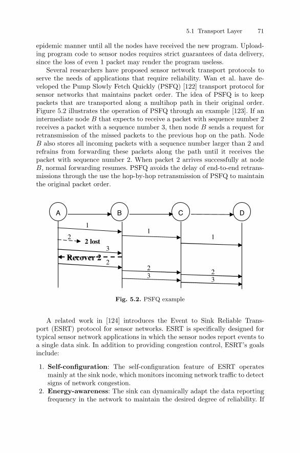
5.1 Transport Layer 71
epidemic manner until all the nodes have received the new program. Upload-ing program code to sensor nodes requires strict guarantees of data delivery,since the loss of even 1 packet may render the program useless.
Several researchers have proposed sensor network transport protocols toserve the needs of applications that require reliability. Wan et al. have de-veloped the Pump Slowly Fetch Quickly (PSFQ) [122] transport protocol forsensor networks that maintains packet order. The idea of PSFQ is to keeppackets that are transported along a multihop path in their original order.Figure 5.2 illustrates the operation of PSFQ through an example [123]. If anintermediate node B that expects to receive a packet with sequence number 2receives a packet with a sequence number 3, then node B sends a request forretransmission of the missed packets to the previous hop on the path. NodeB also stores all incoming packets with a sequence number larger than 2 andrefrains from forwarding these packets along the path until it receives thepacket with sequence number 2. When packet 2 arrives successfully at nodeB, normal forwarding resumes. PSFQ avoids the delay of end-to-end retrans-missions through the use the hop-by-hop retransmission of PSFQ to maintainthe original packet order.
2 lost
Recover 2
1
22
3
11
332
2
A B C D
Fig. 5.2. PSFQ example
A related work in [124] introduces the Event to Sink Reliable Trans-port (ESRT) protocol for sensor networks. ESRT is specifically designed fortypical sensor network applications in which the sensor nodes report events toa single data sink. In addition to providing congestion control, ESRT’s goalsinclude:
1. Self-configuration: The self-configuration feature of ESRT operatesmainly at the sink node, which monitors incoming network traffic to detectsigns of network congestion.
2. Energy-awareness: The sink can dynamically adapt the data reportingfrequency in the network to maintain the desired degree of reliability. If

72 5 Transport and Middleware Layers
the sink detects a higher reliability rate than required, then the sink canreduce the reporting frequency to conserve energy.
3. Collective Identification: In contrast with traditional end-to-end ap-proaches, ESRT adopts a collective identification approach. ESRT’s de-sign builds on the fact that the sink node only needs to collect data aboutevents, and it does not need to know the individual identities of nodes.Thus, end-to-end connections are not supported in ESRT.
Most of ESRT’s decision making functionality is located at the data sink,which has more processing and energy resources than typical nodes. ESRTalways converges to the optimal operating region that balances reliabilityand reporting frequency. Another strength of ESRT is its custom design forsensor networks, which promotes energy efficiency, adaptivity, and reliability.One drawback of this protocol is the variation of reporting frequency withreliability, which may be unsuitable for certain applications that have strictrequirements on data reporting times. Another disadvantage is the assumptionof a single sink, which creates a single point of failure and prevents applicationof ESRT to more general topologies.
The Sensor Transmission Control Protocol (STCP) [125] has many com-mon goals with ESRT: controlled variable reliability; base station controllednetwork; and congestion control. SCTP also considers the energy-reliabilitytradeoffs. The main difference between STCP and ESRT is that STCP adoptsa session-based end-to-end approach like TCP. STCP adopts two differentmechanisms for supporting reliability for continuous and event-driven traffic.For continuous traffic, SCTP determines if packets were lost based on the ex-pected arrival time, which is computed from the data reporting period. Thismechanism may prove difficult to implement in practice because delay be-tween two data update periods may vary considerably due to route changes.For event-driven traffic, the base station provides positive acknowledgementsto the sender. For both continuous and event-driven traffic, the base stationnotifies the sensor nodes of timeouts through negative acknowledgement mes-sages. SCTP also acknowledges that data centric application may require dataaggregation to limit data volume. In this case, the base station does not gen-erate ACK and NACK messages in order to avoid control overhead. STCP’sadoption of flow-based traffic and individual node ID’s supports more granulardata reporting than ESRT. However, its connection-oriented nature may cre-ate too much control overhead in the network. Another drawback is STCP’sunrealistic reliance on timely data reporting from the sensor for determiningtimeouts.
5.2 Middleware
The middleware layer typically provides applications with high level abstrac-tions of the underlying communication system, enabling the application to
5.2 Middleware 73
tune network behavior with minimal information on underlying platforms.In most cases, the middleware layer provides services typically from the OSIsession and presentation layers.
Middleware models tend to provide the middleware layer with visibility tonetwork aspects from all the lower layers, constituting an early and implicitattempt at cross-layer design. Chapters 7 and 8 present more recent cross-layer design approaches that integrate the interaction across layers into thesystem architecture. In this section, we overview the functionality of middle-ware in the context of ad hoc and sensor networks in order to expose potentialcross-layer optimizations involving the middleware layer. We focus here on theinteractions and network management aspects of the middleware, so the soft-ware paradigms that characterize the middleware systems are out of the scopeof this discussion.
The middleware layer lies between the operating system and the applica-tion. Traditional network models run with well-established operating systems,so middleware for these models has clear cut functionality and interfaces. Incontrast, ad hoc and sensor networks are developing research fields for whichoperating systems have not reached the same maturity and stability as tradi-tional networks. As a result, the design of middleware for ad hoc and sensornetworks is still in its infancy.
The remainder of this section visits the design issues in ad hoc and sensornetwork middleware that relate to cross-layer design. Section 5.2.1 exploresthe middleware design issues for ad hoc networks, while Sect. 5.2.2 focuses onsensor network middleware issues.
5.2.1 Middleware for Ad Hoc Networks
Our interest in middleware stems from its similarity to cross-layer design insharing information across layers. The middleware’s role is to observe thestate of lower layers in order to adapt network behavior to the applicationrequirements. The next part of the book reveals that cross-layer design at-tempts to achieve similar goals through a more holistic approach that adoptscross-layering within the network architecture.
Middleware design for ad hoc networks has attempted to build on theextensive middleware concepts for traditional networks. However, several ad-ditional design challenges characterize the development of middleware for adhoc networks [126,128–130]:
• Heterogeneous node resources: Ad hoc and sensor networks may in-clude nodes of varying resources. For example, in an ad hoc network oflaptop computers and hand-held computers, the former have faster CPUs,more memory, and larger batteries. The middleware should be aware ofthese resource differences to better distribute the network load.
• Nature of connections: Wireless connections in ad hoc and sensor net-works exhibit lower bandwidth and higher error rates due to the more
74 5 Transport and Middleware Layers
variable wireless channel. Node mobility also leads to intermittent con-nections, adding another level of complexity. The role of middleware is toinsulate applications from these lower layer details.
• Network partitioning: Dynamic node membership in ad hoc networksmay cause the network to split into several partitions that cannot com-municate. Middleware design must employ mechanisms such as data repli-cation and asynchronous communication to maintain smooth operation ofthe application in anticipation of renewed network connectivity.
For example, Epidemic Messaging Middleware for Ad Hoc Networks(EMMA) [132] is an example of middleware targeting ad hoc networks. EMMAbuilds on the concept of message-oriented middleware (MOM) for traditionalsystems. The attractive feature of MOM is the delay tolerant asynchronoustraffic model, which suits the intermittent connections in highly dynamic adhoc networks. EMMA takes a step in the direction of cross-layering by en-abling the middleware layer to collect information from both the software andhardware components of a node to adapt its behavior. In fact, EMMA disre-gards traditional layer boundaries by considering the middleware and networklayers jointly as the communication layer.
5.2.2 Middleware for Sensor Networks
The diversity of the sensor network application space has motivated the devel-opment of middleware to enable various application to operate on top of sensornetwork platforms. In addition to the challenges of ad hoc network middle-ware, middleware design for sensor networks involves the following additionalchallenges [129,133]:
• Resource limitations: Sensor nodes typically have fewer memory, pro-cessing, bandwidth, and energy resources compared to general ad hoc net-work applications. Middleware components have to be lightweight to fitthe tight constraints of the sensor nodes.
• Cooperative applications: Nodes in sensor networks usually cooperateto achieve a common application goal. Sensor network middleware mustenable nodes to efficiently share their available resources and to performin-network processing when required.
• Scale of deployments: Sensor networks are expected to have hundredsto thousands of nodes, which is at least an order of magnitude higher thantraditional networks and general ad hoc networks. This suggests the needfor scalable middleware that is capable of supporting such large deploy-ments without performance degradation.
• Adaptive fidelity: One of the main tasks of the middleware layer is tomap application performance requirements to protocol parameters. Thehighly dynamic state of sensor nodes may require applications to tradeoffone performance metric for another. The middleware must adapt quickly
5.2 Middleware 75
enough to provide an adaptive bridge between the dynamic network envi-ronment and the application.
As an example of sensor network middleware, consider Middleware LinkingApplications and Networks (MILAN) [129], which attempts to balance QoSrequirements and energy efficiency of sensor networks by optimizing the sensorand network configuration, based on descriptions of application requirements.The application descriptions in MILAN consist of graphs that incorporatestate-based changes in application needs. While traditional middleware sitsbetween the application and the operating system, MILAN considers an ar-chitecture in which the middleware extends into the network protocol stack,to provide support for multiple network platforms. This feature of MILANtouches upon cross-layer design by penetrating the traditional layer boundaryof middleware to enable more profound network optimizations.
6
Application Layer
Real-world applications drive the interest in ad hoc and sensor networks. Adhoc and sensor networks are expected to solve practical problems or to en-hance existing life activities. A wide range of applications motivates ad hocand sensor network development efforts. The unique context of each applica-tion scenario requires highly customized performance guarantees. This chapterexamines the proposed applications and the related performance requirementsthat characterize these applications.
The chapter is structured as follows. Section 6.1 focuses on ad hoc networkapplications, the categories into which they fall, and the application perfor-mance metrics. Section 6.2 examines the sensor network application classes,and their respective performance requirements.
6.1 Ad Hoc Networks
The scope of ad hoc network applications is quite broad. Ad hoc network appli-cations include highly mobile intervehicular networks, delay-sensitive searchand rescue networks, and highly reliable emergency response networks. Inthis section, we first provide an overview of existing application classes ofad hoc networks, along with concrete examples of each application class inSection 6.1.1. We subsequently explore the ad hoc network application per-formance metrics and their relative importance for the relevant applicationclasses in Section 6.1.2.
6.1.1 Ad Hoc Network Application Classes
This section groups ad hoc networks according to their application domain,including [131] military, emergency services, and home/office applications. Thegoal of classifying networks based on their application domain is to unveil thedistinct application characteristics of ad hoc networks and how they relate
78 6 Application Layer
to lower layer behavior. As ad hoc networking is still an emerging field, weexpect the scope of ad hoc network applications to keep on rapidly expanding.
Military Applications
Military applications have motivated early research on ad hoc networks. Theability to quickly set up a network among military units in hostile territorywithout any infrastructure support can provide friendly forces with a consider-able tactical advantage on the battlefield. For instance, each soldier can carrya mobile device that represents one of the mobile nodes in an ad hoc networklinking all soldiers, tanks, and other vehicles. Recent advances in robotics havealso motivated the idea of automated battlefields in which unmanned fightingvehicles are sent into battle. Supporting military applications requires self-organizing mechanisms that provide robust and reliable communication indynamic battle situations.
Emergency Services
Another promising application area for ad hoc networks is emergency services,including search and rescue and disaster recovery operations. As an exampleof search and rescue, consider an airline that attaches small wireless devicesto the life jackets under each seat. Suppose that the plane has mechanicalproblems and has to make an emergency landing in the water. Once searchand rescue teams arrive at the landing site, they are provided with detailedinformation about the location (the coordinates and potentially the depth)of the victims through the transponders. As a result, the rescue teams canmore effectively locate and reach the victims. The mobile devices could alsomonitor the vital signs of victims, such as heart rate or breathing rate, toprioritize the rescue of victims that are still alive.
A similar application arises when disasters, such as earthquakes, blackouts,or bombings occur. The disaster may destroy existing communication infras-tructure, preventing critical contact among emergency workers. The emer-gency response teams can set up ad hoc networks quickly to replace the de-stroyed infrastructure, enabling the teams to better coordinate their efforts.
Home, Office, and Educational Applications
Ad hoc networks also have applications in home and office environments. Thesimplest and most direct application of ad hoc networks in both homes andoffices is the networking of laptops, PDAs and other WLAN-enabled devicesin the absence of a wireless base station. Another home application that fallswithin the Personal Area Network (PAN) class is wire replacement throughwireless links, as in Bluetooth. All periphery devices can connect to a computerthrough wireless Bluetooth links, eliminating the need for wired connections.
6.1 Ad Hoc Networks 79
Ad hoc networks can also enable streaming of video and audio among wire-less nodes in the absence of any base station. For instance, UWB provides asufficiently high bandwidth (in the order of Gb/s) to support several mul-timedia streams. UWB-equipped nodes can autonomously set up an ad hocnetwork to stream high quality video and audio between several computersthrough wireless UWB connections.
Educational and recreational activities can also benefit from ad hoc net-works. For example, students attending a classroom can use their laptops toobtain the latest class material from a professor’s laptop as the class pro-gresses. On the recreational side, the mobility and nomadic nature of ad hocnetworks enables richer multi-user games that can incorporate user mobilityand proximity into the virtual game environment.
6.1.2 Application Performance Metrics
This section has so far explored potential ad hoc network application sce-narios. We now examine the typical ad hoc network application performancemetrics, and their relation to the application scenarios. Most of the applicationperformance metrics are highly dependent on parameters and mechanisms atlower layers in the communication stack, revealing potential for cross-layeroptimizations.
Prior to presenting the application performance metrics, we define thefollowing traffic types for ad hoc networks:
• Continuous traffic: refers to continuous data flow along a link or path• Synchronous traffic: refers to time-sensitive data flow• Bursty traffic: refers to generic application data without any specific tem-
poral pattern
Reliability
Ad hoc network applications that cannot afford any data loss emphasize re-liability as a main performance requirement. Military applications and emer-gency management services both fall into this category, since the loss of anydata in these applications may endanger human life. As the previous chaptersreveal, many lower layer network mechanisms provide reliable data delivery,such as an Acknowledgement message at the MAC or the transport layers.However, applications that run over unreliable communication stacks mayneed to define their own application-level reliability mechanisms, such as ap-plication layer acknowledgement mechanisms.
Throughput
Ad hoc network applications with continuous traffic, such as video streamingor multi-user gaming, require a guaranteed level of throughput. Applications
80 6 Application Layer
typically only specify their throughput requirements with the assumption thatlower layer mechanisms are capable of satisfying these requirements. Provid-ing throughput guarantees in ad hoc networks is challenging because of nodemobility, highly variant channels, and the connectionless nature of most adhoc network communications. As Section 5.2 describes, replicating the dataat several nodes can minimize the effect of node mobility on end-to-end appli-cation throughput. However, data replication may not work if node velocitiesexceed a certain level. Another useful concept that promotes throughput guar-antees for ad hoc network applications is the reservation of bandwidth alongvirtual links or paths, which is also subject to mobility considerations.
Delay
Synchronous traffic applications also require delay related guarantees. Astreaming application, such as video or audio streaming, may require limits onthe end-to-end delay or the interframe delay variance. Military networks anddisaster relief networks also place strict constraints on end-to-end delay sincetardy data in these critical and highly dynamic situations may become use-less. In contrast, standard data communications applications such as internetbrowsing or ftp may tolerate delay.
Provision of delay guarantees in ad hoc networks is challenging becauseof their highly dynamic nature. Implementation of delay mechanisms at theapplication layer is not desirable, since end-to-end delay is highly dependenton lower layer activities such as medium access (collisions and backoffs), rout-ing (queueing and forwarding), and transport (congestion and flow control).Most current ad hoc networks exploit algorithms at lower layers, such as pri-orities, scheduling, and reservations, in an attempt to deliver time-sensitivedata within the delay bounds.
Energy Efficiency
The mobility of battery-powered nodes in ad hoc networks may prevent fre-quent replenishment of the limited energy resources at each node. The limitednode resources motivate the design of energy efficient mechanisms for ad hocnetworks at every layer in the network stack. Although applications do notdirectly manage energy-related issues, they can specify energy bounds or re-quirements. For example, applications can specify minimum network lifetimerequirements.
Energy efficiency is certainly a cross-layer aspect that can benefit all classesof ad hoc network applications. For example, tuning of modulation rates atthe physical layer, adaptation of duty cycles at the MAC layer, and choosingroutes that maximize network lifetime at the network layer can all yield energysavings. However, the inherent tradeoff between energy efficiency, delay, andthroughput in ad hoc networks may limit the potential energy optimizations.
6.1 Ad Hoc Networks 81
Applications with bursty traffic, such as home and office ad hoc networks,may be able to tolerate considerable delay in order to preserve valuable nodeenergy resources. Other applications with continuous or synchronous trafficthat prioritize reliability or delay provide the potential for only limited energyoptimization.
Data Accessability
Timely access to data is crucial for supporting time-sensitive applicationswith synchronous traffic. Because of dynamic node membership and nodemobility, providing applications with continuous access to data remains anopen research issue. A potential solution to the data accessability problem isthe selective replication of data across several nodes to ensure that at leastone node can service any requests for the data. Delay bounds in synchronoustraffic applications, for example in multimedia applications, determine theoptimal degree of data replication. If the delay bounds are too small, then theoverhead of data replication may overweigh its benefits.
Fairness
Fair access to the network among multiple applications that run concurrentlyis yet another performance goal for ad hoc network applications. Reservationsof communication resources by high-priority traffic, such as synchronous orcontinuous traffic, may cause bandwidth starvation of applications with lowerpriority traffic. Applications should typically specify the extent of fairness tobe enforced by lower layers. For example, the network can allocate 60% of theavailable bandwidth to streaming traffic and 40% to bursty traffic. The net-work can further specify the allowable bandwidth allocations among streamsof the same traffic class, to ensure fair access to communication resources. Nat-urally, enforcing fair access in ad hoc networks adds another level of designand implementation complexity for the network mechanisms.
Multicast Support
The channel in ad hoc networks is inherently a broadcast medium, so allnodes within the vicinity of a transmission receive the signal at the physicallayer. However, broadcasting at higher layers is not energy-efficient since allthe unintended receivers of a signal waste energy in processing the packetbefore discarding it. At the other extreme, nodes may address specific neigh-bors through unicast transmission. Unicast transmissions currently dominateresearch for ad hoc networks. In between broadcasting and unicasting, mul-ticasting provides an alternative in which a node targets a designated groupof nodes to process the received signal. For instance, gaming and enterpriseapplications of ad hoc networks can exploit multicast groups for richer inter-actions among users.
82 6 Application Layer
The network layer is traditionally responsible for implementing multi-castmechanisms. However, several works have explored application layer overlaysfor forming multi-cast groups in ad hoc networks [134, 135]. The attractiveaspect of application layer multicast support is that it avoids changes to thenetwork layer and it does not involve increased state maintenance at interme-diate nodes. The drawbacks of application layer multicasting are the possibil-ity of redundant packets at intermediate nodes in the mulicast tree, and theuse of sub-optimal routes.
6.2 Sensor Networks
This section first considers the broad sensor network application classes basedon their data dissemination strategies, providing examples for each class inSect. 6.2.1. The discussion in Sect. 6.2.2 then focuses on the application per-formance layer requirements for sensor networks.
6.2.1 Data Dissemination
Sensor networks collect data from their physical environments, process thedata, and eventually report it back to the network user. We refer to thisset of actions as data acquisition and dissemination. Three broad classes ofsensor network applications emerge depending on the factors that drive dataacquisition and dissemination: time-driven; event-driven; or demand-driven.
Time-driven Sensor Networks
We motivate the discussion on time-driven sensor networks with an exampleapplication. Consider an underwater network of sensors that monitors physi-cal indicators, such as temperature, salinity, pressure, and wave direction, todetermine the level of pollution in the water. The network consists of sev-eral subsurface nodes that are deployed to sense the underwater environment.One of the nodes, referred to as base station or data sink, lies on the surfacewithin communication range of the underwater nodes. The base station is alsoa gateway node that can communicate with the underwater nodes and a relaystation at the shore. Because changes in underwater pollution levels can varywithin a time scale of minutes, the underwater nodes sample their sensorsand send the data via the base station every few minutes. Monitoring the un-derwater environment at fixed time intervals provides environmental expertsthat will analyze the data with a well-defined data granularity for predictingpollution in the water.
We now present a more general description of time-driven sensor networks.In time-driven networks, sensor nodes collect and report data from the physi-cal environment periodically. The period between two consecutive data pack-ets from a particular sensor node is referred to as the “data sampling fre-quency” or the “data reporting frequency”. Each sensor node typically sets

6.2 Sensor Networks 83
an internal timer to manage the periodic data sampling and reporting. Thedata reporting frequency may be either static or dynamic. Applications thatset a static data reporting frequency do so prior to network deployment to pro-vide the user with data at fixed length intervals. In contrast, applications witha dynamic reporting frequency enable nodes to change their data reportingfrequency during network deployment.
The periodicity of information flow in time-driven sensor networks pro-vides for more predictable long-term behavior of the network. Designers canexploit the periodicity of information flow to optimize network performance.For example, an algorithm that is aware of the data reporting frequency canschedule transmissions of non-interfering nodes in such a way that maximizesspatial reuse and bandwidth utilization, while minimizing energy consump-tion (see Ch. 9). Time-driven sensor networks represent a simple model inwhich the nodes mostly report data and perform minimum data processing.Most of the processing takes place once the data reaches the data sink, whichtypically includes a larger computer with more resources. This class of sensornetwork applications requires minimal processing and memory resources atindividual nodes. However, some applications require smarter sensor nodesthat are able to partially process sensed data and to make appropriate deci-sions autonomously. Such applications allow the nodes to respond to eventsin the environment or to user queries.
Event-driven Sensor Networks
Event-driven data dissemination is a reactive model that closely fits the re-quirements of many sensor network applications. Nodes in event-driven sensornetworks do not send their data periodically. Instead, nodes can adjust theirdata reporting behavior based on certain network events. Events are definedby setting thresholds for the sensed values. Once a sampled value exceeds aparticular threshold, the node determines that the associated network eventhas occurred and it adapts its behavior accordingly.
We illustrate the operation of an event-driven sensor network through anexample. Consider a network of sensors that is deployed for monitoring seis-mic activity along a fault line, as an early warning system for earthquakes.Earthquakes may occur several years apart, so the network should providelong-term unattended operation. Time-driven monitoring of the fault line isnot a suitable choice in this application. Setting a data reporting frequencythat is too high would deliver high data granularity, but it would also wastevaluable energy resources for frequent transmissions, causing the nodes to de-plete their batteries quickly. A small data reporting frequency would solvethe network longevity problem, but the data granularity may be too low forreporting relevant seismic events. Instead, the nodes should only report worth-while data, which they can determine based on thresholds for sensed physicaldata. For example, if a node detects that vibration has exceeded the thresholdvalue, it determines that a seismic event is taking place and it increases its
84 6 Application Layer
data reporting frequency for the duration of the event. Other nodes in thevicinity of the seismic activity follow the same behavior, while nodes that arenot aware of the seismic event do not change their behavior.
As the above example shows, nodes in event-driven networks can assumedifferent roles during deployment. The application must provide specificationsof possible roles of nodes, and the network must support and adapt dynamicnode roles. In particular, role-aware network mechanisms can use the cross-layer role information to optimize their configuration.
In many event-driven sensor networks, such as networks to detect forestfires or intrusions, data must arrive as quickly as possible to the user, so lowlatency is key for event-driven sensing applications. The event-driven modelis a suitable reactive adaptation of the time-driven model, in which events inthe deployment area drive data reporting. However, the event-driven modeldoes not fit applications that require user control over network behavior.
Demand-driven Sensor Networks
While events in the operating environment drive data reporting in event-driven sensor networks, demand-driven sensor networks enable network enti-ties, such as the end-user or software components within the network, to querythe nodes for sensor data. Queries may be either name-based or attribute-based. Name-based queries specify the address or name of a particular set ofsensor nodes from which data is required. Instead of targeting explicit sensorgroups by name or address, attribute-based queries specify the attributes ofthe node targeted by the query.
We now present a brief example of a demand-driven network. Consider anetwork of wireless sensor nodes for traffic monitoring. Sensors are deployedbelow the tarmac on the highway to report traffic speeds and to infer trafficcongestion. A user could issue the following query: What is the traffic on In-terstate 405 at the Atlantic Avenue exit? The network propagates the querytowards the sensors at Atlantic Avenue, which sample their sensors and reportthe data back to the user. This is an example of a name-based query. Alter-natively, the user could submit the following attribute-based query: What arethe points of congestion on Interstate 405 between Atlantic Avenue and Su-pelvida Boulevard? Only the nodes that detect slow traffic speeds in the areabetween Atlantic and Supelvida report their data in response to this query.
The data dissemination models for sensor networks are not mutually ex-clusive and they can be combined to provide a richer set of data disseminationoptions. For example, combining the time-driven and event-driven models canallow all nodes to report data infrequently, and nodes that detect an interest-ing event can report data with a higher frequency.
6.2.2 Application Performance Metrics
A single entity generally deploys a sensor network to monitor a physical space.Network users are concerned with the high level application performance of
6.2 Sensor Networks 85
the network. Common requirements for sensor network applications includereliability, system lifetime, data freshness, and data resolution. The remainderof this section explores the application layer performance metrics for sensornetworks in relation to the application classes in Section 6.2.1.
Reliability
Many sensor network applications require reliable data delivery. For exam-ple, a sensor network that monitors toxic leaks in an industrial facility mustensure without any doubt that any leak event is reported. From an applica-tion’s perspective, reliable data delivery guarantees that transmitted data isreceived at its intended destination. Providing reliability to sensor networkapplications requires additional control messaging, such as handshakes andacknowledgements, at lower layers in the communications stack.
Network Lifetime
The deployment area of sensor networks may not be readily accessible. Mil-itary sensor networks may be deployed in hostile territory to monitor troopmovements. Environmental sensor networks might monitor physically harshenvironments, such as rainforests, volcanoes or deep ocean waters. Networksthat monitor the structural integrity of bridges may embed the sensors withinthe concrete, making it very difficult to reach the sensors.
Because of the inaccessibility of deployment areas of many sensor networks,it is desirable to prolong the network lifetime to avoid replacing or rechargingthe sensor nodes frequently. Maximizing the network lifetime often requiresenergy efficient mechanisms at several lower layers across the network stack,such as support for adaptive duty cycles, power-aware routing, and adaptivetransmission powers.
Delay
Delay is an important metric for some sensor network applications, such asreal-time monitoring sensor networks, emergency response networks, targettracking networks, or industrial automation networks. Delay in sensor net-works is typically intermittent and highly variable due to sensitivity of intern-ode communications to environmental changes.
There are two delay components from a sensor network application’s per-spective: data freshness and response time. Data freshness indicates how re-cent the reported data is. The more recent data typically reflects the currentstate of the deployment area more accurately. The response time indicates thenetwork application’s capability to respond to environmental events or userqueries within a given interval of time. For instance, a military applicationmight set tight constraints on query response time to ensure that friendlytroops can react quickly enough to enemy movements.
86 6 Application Layer
Data Resolution and Detection Probability
The detection probability refers to the probability that the sensor networkcan detect the occurrence of a relevant event within the deployment area.The data resolution refers to both the spatial and temporal granularity ofthe sensed data, which depends on the number of sensors that can monitor aparticular point in the deployment area and on the data reporting frequencyrespectively.
Both the detection probability and the data resolution depend on themethod and manner of sensor node deployment. The density of sensor nodesplays a major role for event detection. Naturally, sensor density involves atradeoff with network cost and scalability. The network topology should bedense enough to ensure a sufficient data resolution for any relevant eventwithin the deployment area. On the other hand, network designers must limitsensor density to minimize the scale and the monetary cost of the network.
The sensor deployment strategy also affects detection probability and dataresolution. Sensor nodes may be regularly spaced within the deployment areato provide uniform data resolution. Alternatively, the network user may placemore sensor nodes in a certain region of particular interest within the deploy-ment area to provide higher data resolution in that region. A related issueis the accessibility of the deployment area. If the network user can deter-ministically deploy the nodes in the deployment area, then any deploymentstrategy will do. However, the deployment area may not be readily accessible.For example, a military application may require sensor deployment in enemyterritory, in which case the sensors are dropped over enemy territory froma plane. Obviously, such a deployment strategy does not allow deterministicsensor placement. Instead, the sensors can be dropped at roughly equal dis-tances in order to ensure with some probability that the network can detectrelevant events.
Node mobility and node failures are two factors that contribute to dynamicnetwork topology, affecting detection probability and data resolution. Reasonsfor node failures include unreliable sensor node hardware and the limited nodebattery resources. Thus, it is highly likely that some sensor nodes will fail dur-ing a long-term deployment. Sensor density and placement strategies shouldconsider the expected node failure rate prior to deployment to ensure bothacceptable data resolution and detection probability. Node mobility also af-fects the detection probability in a sensor network. The movement of sensornodes may cause an initially acceptable network topology to provide an unsat-isfactory level of detection probability and data resolution. In mobile sensornetworks, the application may have to specify acceptable ranges for detectionprobability and data resolution. The acceptable range would depend on thedegree of mobility and the maximum speed of the nodes.

Part II
Cross-Layer Approaches
7
Cross-Layer Design
This part of the book focuses on cross-layer design for ad hoc and sensornetworks. In this chapter, we build up the case for cross-layer approachesthrough an examination of the unique requirements of ad hoc and sensornetworks, and we outline guidelines for cross-layer models for these networks.The next two chapters focus on existing cross-layer approaches. Chapter 8examines proposed cross-layer architectures for ad hoc and sensor networks,while Chapter 9 focuses on applied cross-layer approaches.
This chapter is structured as follows. Section 7.1 provides a comprehensivedefinition of cross-layer design approaches. Section 7.2 presents existing workon cross-layer approaches for traditional networks. Section 7.3 motivates cross-layer design for ad hoc and sensor networks. Finally, Section 7.4 presents thecross-layer design guidelines for ad hoc and sensor networks.
7.1 Cross-Layer Design: A Definition
Layered communication approaches typically separate communication tasksinto several layers, with a clear definition of the functionality of each layer. Ina layered communication stack, interaction among layers occurs through well-defined standardized interfaces that connect only the neighboring layers in thestack. Figure 7.1 depicts the traditional layer interaction through standardizedinterfaces in a strictly layered communication stack.
In contrast, cross-layer approaches attempt to exploit a richer interactionamong communication layers to achieve performance gains. Srivastava andMotani [139] have recently proposed the following definition for cross-layerdesign: “Protocol design by the violation of a reference layered communica-tion architecture is cross-layer design with respect to the particular layeredarchitecture.” The basic premise of this definition is that cross-layer protocoldesign by definition violates the strictly layered interfaces of a reference lay-ered communication architecture. However, Srivastava and Motani’s definitiondoes not encompass all of the existing cross-layer approaches. For example,
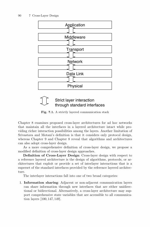
90 7 Cross-Layer Design
Application
Middleware
Transport
Network
Data Link
Strict layer interaction through standard interfaces
Physical
Fig. 7.1. A strictly layered communication stack
Chapter 8 examines proposed cross-layer architectures for ad hoc networksthat maintain all the interfaces in a layered architecture intact while pro-viding richer interaction possibilities among the layers. Another limitation ofSrivastava and Motani’s definition is that it considers only protocol design,whereas Chapter 9 and Chapter 8 reveal that algorithms and architecturescan also adopt cross-layer design.
As a more comprehensive definition of cross-layer design, we propose amodified definition of cross-layer design approaches.
Definition of Cross-Layer Design: Cross-layer design with respect toa reference layered architecture is the design of algorithms, protocols, or ar-chitectures that exploit or provide a set of interlayer interactions that is asuperset of the standard interfaces provided by the reference layered architec-ture.
The interlayer interactions fall into one of two broad categories:
1. Information sharing: Adjacent or non-adjacent communication layerscan share information through new interfaces that are either unidirec-tional or bidirectional. Alternatively, a cross-layer architecture may sup-port comprehensive state variables that are accessible to all communica-tion layers [100,147,149].
7.2 Cross-Layer Design for Traditional Networks 91
2. Design Coupling: Design of new protocols or algorithms may try toexploit the features or avoid the weaknesses of existing mechanisms [159,172]. More extreme cross layer approaches can partially or completelyintegrate the functionality of adjacent layers [160].
With this formal definition of cross-layer design, we proceed to follow thehistorical development of cross-layer design approaches in the next section.
7.2 Cross-Layer Design for Traditional Networks
Cross-layer design has its roots in infrastructure wireless networks. Earlycross-layer models for wired networks have shown the benefits of cross-layerprotocol interactions [136,137]. One of the first cross-layer proposal addressesTCP’s failure in distinguishing network congestion from communication er-rors, which leads to invocation of the congestion control mechanism for bothcases, as Section 5.1.1 discusses. This drawback of TCP is more pronouncedfor wireless networks, even infrastructure wireless networks, where the wirelesschannel exhibits both short-term and long-term variations [141]. To remedythis problem, future versions of TCP are expected to support an ExplicitCongestion Notification [142] (ECN) bit. Routers can set the ECN bit to indi-cate that packets have experienced congestion. When the destination receivespackets with the ECN bit set to one, the destination notifies the sender of thecongestion so that the sender can reduce its transmission rate. Because thenetwork layer at an intermediate node sets the ECN bit and transport layerat the destination reads it, the ECN bit represents a cross-layer interaction.
Another example is the enhancement of the Mobile IP hand-off with linklayer information. Hand-off in Mobile IP networks occurs on detection of net-work changes at the network layer. Because network layer detection may betoo slow, Sanmateu et al. [138] propose the use of signal strength informationfrom the physical layer on the active links to reduce the hand-off latency.
The majority of cross-layer optimizations for traditional networks adopt aninformation sharing approach. Information sharing approaches involve minormodifications to existing models, and they can yield significant improvementsin performance. Existing literature [139, 143] on cross-layer design for infras-tructure wireless networks has reached a consensus on the benefits of richinformation sharing and interaction among layers. While design coupling mayprovide for deeper optimizations [139], it also moves further away from thelayering models. As a result, design coupling trades off the performance gainsfor almost all of the interoperability and modularity benefits of layering. De-sign coupling has so far proved useful for optimizations that address particularscenarios [160] or specific technologies [172].
In this ongoing tension between the generality benefits of layered designsand the efficiency gains of cross-layer designs, a middle ground approach that
92 7 Cross-Layer Design
seems to balance the tradeoffs emerges. The middle ground approach essen-tially adopts information sharing in an attempt to preserve the current lay-ered models while enhancing them with richer interactions among layers tooptimize performance. By preserving layering, the models keep the interoper-ability benefits. Support for richer interactions enables a closer coordinationbetween the communication layers. In Chapter 8, we examine several sucharchitectures for both ad hoc and sensor networks that adopt this middleground approach. Before discussing these proposed cross-layer models for adhoc and sensor networks, the next section motivates cross-layer design forthese networks.
7.3 Why Cross-Layer Design for Ad Hoc and SensorNetworks?
This section investigates the factors that have led researchers to consider cross-layer design for ad hoc and sensor networks. We begin this section with ananalogy between government interactions and data communication as a sim-ple introductory motivation for cross-layer design. Next, we formally presentthe challenges that have motivated cross-layer design for ad hoc and sensornetworks.
7.3.1 An Analogy
In this example, we draw an analogy between the interaction within a govern-ment structure and the interaction within a network. Consider first how highlycentralized governments, such as the government of France, operate. Most, ifnot all, of the major executive decisions are taken by the central government,which has a well-defined hierarchy of employees. The bureaucracy specifieswell-defined channels through which government employees at each level inthe hierarchy interact with lower-level employees, higher-level employees, andpossibly with citizens. For example, a mid-level manager in the ministry ofhealth can give directives and receive reports from employees under him thatdirectly interact with the citizens, and he can create reports for and receive di-rectives from the higher-level manager. Within this structure, the higher levelgovernment officials and the citizens have no direct interaction. The employeehierarchy in this example resembles layered architectures that define stan-dard interfaces between neighboring layers of the communication stack andthat disallow communication between non-neighboring layers. For instance, intraditional layered models, the network and transport layers have no directinteraction with the physical layer.
Now consider the other extreme of government represented by the directdemocracy in a federated government. Take Switzerland, for example, whichhas a federated government of three cantons that applies the concept of direct
7.3 Why Cross-Layer Design for Ad Hoc and Sensor Networks? 93
democracy to hold elected officials immediately accountable for all their ac-tions. One factor that has strengthened direct democracy in Switzerland is thefederated government system, which allocates far more power to the regionalcanton governments than the federal government. Shifting the governmentadministration activities to the local governments enables a richer interactionbetween the people and the government officials, as the citizens can keep trackof and interact meaningfully with elected officials in smaller districts. In fact,the richer interaction between the constituents and the government becomescrucial to the government efficiency with the increased distribution of gover-nance activities. The smaller tax revenues of local administrations highlightthe need for making efficient use of these resources, as any waste of tax rev-enue will be directly felt by the citizens. To complement the highly federatedgovernment model, Switzerland has the most prominent example of directdemocracy in the world. In the past 120 years, the system has enabled Swisscitizens to vote on 240 referendums on key issues [140]. The direct democracysystem also enables citizens to frequently contact and select elected officials,and to hold them accountable for all their actions while in office.
In our analogy, the local governments in the Swiss system represent nodesin ad hoc networks, and the citizens and government officials at differentlevels represent the protocol layers. Two concepts from the federated directdemocracy system are relevant for ad hoc and sensor networks: distributeddecisions and richer interactions. The distributed decisions that take place inthe federated government model resemble the distributed network manage-ment decisions by individual nodes in ad hoc and sensor networks. Just likein the Swiss system, the efficient performance of the node may benefit, andin some cases may even require, richer interactions among the communicationlayers of the node in the network. Cross-layer design for ad hoc and sensor net-works aims to provide richer interlayer interaction within a node to improvethe node’s performance.
7.3.2 Motivating Factors
Having motivated cross-layer design through the government analogy, we nowformally present the factors that motivate cross-layer design for ad hoc andsensor networks. We will first examine the motivating factors for general adhoc networks, followed by factors that are specific to sensor networks.
The motivating factors for cross-layer design for ad hoc networks include:
1. Cross-Layer Aspects: Nodes in ad hoc networks must manage severalperformance aspects, such as power management, system management, se-curity, and discovery that cut across traditional layers. For instance, bothmedium access and routing decisions have significant impact on powerconsumption, and the joint consideration of both can yield more efficientpower consumption. The strict separation of layers and standardized in-terlayer interfaces in traditional approaches do not enable sufficient inter-action among layers to make joint decisions to optimize these cross-layer
94 7 Cross-Layer Design
aspects. This has led to the proposal of new interaction models to supportcross-layering, ranging from a more relaxed information flow and sharingbetween layers to full-fledged merging of layer functionalities.
2. Distributed State: Unlike traditional infrastructure models where basestations have a global view of network state, the network state in ad hocnetworks is generally distributed across the nodes. Each node forms itsown local view of state, representing a partial view of the overall networkstate. In most cases, it is not feasible to collect network state at any onenode, which prevents the use of any centralized optimization algorithms.As such, each node can run distributed algorithms locally using its partialview of network state. Distributed algorithms can exploit a cross-layerdesign to enable each node to perform fine-grained optimizations locallywhenever it detects changes in state.
3. Mobility: Mobility introduces an additional challenge for ad hoc networkdesign. Imagine if all the Internet routers were mobile. Routing protocolswould have to cope with this mobility by constantly adapting routing stateto the changing router positions. Now consider mobility in the context ofad hoc networks, where no node has global view of network state. Mobilitymanagement poses an additional challenge to the battery-powered nodesin ad hoc networks, which have to adapt their behavior to the chang-ing node locations. Mobility causes changes for the physical layer (e.g.interference levels), the data link layer (e.g. link schedules), the routinglayer (e.g. new neighbors), and the transport layer (e.g. connection time-outs). As such, a cross-layer design enhances a node’s capability to manageits resources in mobile environments.
4. Wireless Link Properties Wireless links are more susceptible thanwired links to interference variations and channel errors. One classic ex-ample is the TCP congestion control problem over wireless links in whichTCP misinterprets a packet loss due to channel error as a sign of conges-tion. Wireless links are also more vulnerable to security attacks becauseof easy access to the wireless channel. Providing higher layers with aware-ness of the wireless link status enables nodes to adapt their configurationbetter to physical layer properties. For example, a routing protocol thatdetects a drop in quality of a particular wireless link can create a newroute to divert traffic to another wireless link.
5. New Communication Modalities: Ad hoc network design can exploitthe broadcast nature of the channel to enhance performance. For exam-ple, nodes can snoop on neighboring transmissions in order to evaluatethe quality of links with neighbors. Antenna arrays also enable the re-ception of multiple packets simultaneously on the wireless channel. Datapackets corresponding to several connections could arrive simultaneouslyat a node. The close coordination of the routing, data link, and physicallayer can ensure the timely forwarding of data for all the connections. Thebroadcast nature of the wireless channel also provides fertile ground forsupporting multicast interactions.
7.3 Why Cross-Layer Design for Ad Hoc and Sensor Networks? 95
6. Inherent Layer Dependencies Several interlayer dependencies moti-vate cross-layer design for ad hoc and sensor networks. The data link androuting layers in ad hoc networks exhibit both variable and algorithmicinteraction [144], suggesting the need for design coupling of these layers.The data link layer is also closely related with the physical layer. If pro-vided with current channel conditions, the data link layer can adapt errorcontrol mechanisms in a dynamic manner, thereby improving through-put [145].
7. Resource-Constrained Nodes The form factor of mobile nodes for adhoc networks keeps decreasing, imposing the use of smaller batteries forthese nodes. The relatively slow improvement in battery technology im-plies that the nodes must interact in an ultra-efficient manner to maximizethe lifetime of the battery. Cross-layer design approaches can expose powerrelated variables at several layers, enabling nodes to efficiently utilize theirenergy resources.
The above factors apply to both general ad hoc networks and sensor net-works. The following additional factors characterize cross-layer design for sen-sor networks:
1. Global Performance Guarantees: Nodes in sensor networks typicallycollaborate to achieve a common network goal. As such, sensor networksmust support the enforcement of performance guarantees on a network-wide scale. The absence of a central controller that has a global view ofnetwork states requires that the distributed algorithms running at thenodes adhere to the global performance policies. Therein lies the mainchallenge in the design of communication protocols for sensor networks.Global performance policies can only be enforced through local decisionsmade at individual nodes in a greedy and distributed fashion. Efficientnetwork operation requires that the local algorithms that optimize globalperformance adapt to the local state at each node. The local algorithmsshould strike a balance in adapting to the dynamic local node states, whileadhering to the global optimization policy.
2. Application-Specific Policies: The semantic definition of what consti-tutes “good performance” varies greatly between different sensor networkapplications. For example, a sensor network that monitors pollution levelsin a watershed [14] prioritizes network longevity to avoid frequent retrievaland recharging of node batteries. In contrast, a sensor network for toxicleak monitoring in a factory emphasizes reliability and delay to guaran-tee that any leak event is reported promptly. The wide range of possiblesensor network applications and the application-specific performance re-quirements of each application suggest the need for a general model thatis tunable to each application. The general model should ensure that therelative impact of quality of service metrics, which inherently cut acrosslayers, can be tuned to suit particular applications.

96 7 Cross-Layer Design
3. Platform-Specific Properties: Because they interface the physicalworld with the digital domain, sensor network operation inherently de-pends on the hardware platform that performs the sensing and commu-nication. While the specifications of each sensor network platform varywidely, the platforms must provide higher layers and applications withsufficient control over sensing and communication behavior. Successful de-sign strategies should hide the differences of various hardware platformsfrom higher layers (for instance through hardware abstraction layers) inorder to enable efficient mapping of application performance goals to thephysical layer parameters. Cross-layer models provide a richer interactionset for mapping the abstract application performance requirements to thephysical platform-specific properties [149].
4. Unattended Operation: Most sensor network applications require unat-tended operation, so the network nodes must independently determinehow to react to mobility, loss of connectivity, or energy depletion. Cross-layer approaches provide nodes with unprecedented visibility about theircurrent resources and processes, which contributes favorably to node au-tonomy and self-configuration.
This section has identified the factors that motivate cross-layer design forad hoc and sensor networks. The next section builds on these factors to developgeneral guideline for cross-layer design in ad hoc and sensor networks.
7.3.3 Design Challenges
Cross-layer design also involves risks that, some researchers would argue, mayoutweigh its benefits. Kawadia and Kumar [146] emphasize the ongoing ten-sion between performance and architecture: while cross-layer design offersshort-term performance benefits for a particular system over traditional ar-chitectures, it also limits the modularity and interoperability offered by archi-tectures. They identify the following challenges for cross-layer design:
1. Unstructured Code: The implementation of several cross-layer designoptimizations within a system may lead to spaghetti-like code that is un-structured and thus difficult to maintain. The unstructured code may stifleinnovation as it makes it harder to modify or upgrade existing systems.It also raises questions on the proliferation and longevity of the system.Finally, the unstructured code could eventually lead to an increase in per-unit cost. All of these factors can be regarded as long term performancemetrics that may be adversely affected by cross-layer design.
2. Multiple Interactions: Cross-layer design opens the floodgate of infor-mation flow across layers, raising concerns on multiple, sometimes subtle,interactions among existing layers. For example, a cross-layer approachmay determine that current conditions necessitate configuration A at therouting layer and configuration B at the MAC layer, although configu-rations A and B may have unknown interactions that lead to degraded

7.4 Cross-Layer Design Guidelines 97
network behavior. A major challenge of cross-layer design is the clear iden-tification and exploration of the possible dependencies and interactionsamong the system processes at different layers.
3. Short-term Benefits: According to Kawadia and Kumar, cross-layerdesign offers performance benefits for a particular system, yielding short-term gains. In contrast, an architecture offers a model for sustained in-novation in a system, so it offers long-term gains. Their contention isthat the long-term gain of architecture overweighs the short-term gain ofcross-layer optimizations. However, many ad hoc and sensor network ap-plications are quite specific in nature, so the short-term performance gainsof cross-layer design may be far more important for the network user tomake efficient use of scarce node resources.
4. Holistic Perspective: Because cross-layer optimization involves depen-dencies among other system processes and other systems, cross-layer de-signers must consider the impact of their design with a holistic view thatincludes the long-term development and innovation considerations.
The above challenges suggest that the benefits and opportunities for im-proving performance through cross-layer design should be embraced cau-tiously through preservation of a form of architectural framework to providemodularity, define interactions, and drive innovation. The next section at-tempts to outline the guidelines for cross-layer design that can balance thesedesign tradeoffs between architecture and performance.
7.4 Cross-Layer Design Guidelines
The discussion in the previous sections yields design guidelines for ad hoc andsensor network cross-layer design. In this section, we examine the guidelinesfor efficient and deployable cross-layer models for ad hoc and sensor networks.
7.4.1 Compatibility
The quick development of the Internet has shown the importance of an archi-tecture in ensuring interoperability and compatibility among users on a globalscale. Although development of new protocols has skyrocketed recently, adhoc and sensor networks need a reference architecture [147,149] within whichprotocols developed by one research group can interoperate with other devel-opment efforts. In addition to providing compatibility, a successful referencearchitecture must enable flexible cross-layer interaction to support fine-grainedoptimizations.
Backward compatibility with IP-based networks is another considerationfor designers of cross-layer approaches for ad hoc and sensor networks. Thepervasiveness of Internet-enabled nodes provides a fertile gateway throughwhich ad hoc and sensor network nodes can communicate globally. Many ad
98 7 Cross-Layer Design
hoc networks, such as networks of laptops and PDAs, can provide each nodean individual IP address for directly interfacing with other Internet nodes. Insensor networks, nodes may rely on a gateway node, usually the data sink, foran interface with the Internet.
7.4.2 Richer Interactions
Cross-layer design must address two types of interactions: interlayer interac-tions; and internode interactions. The interlayer interactions deal with theallowable information exchange between communication layers within eachnode. Cross-layer approaches must specify the implementation details of theinterlayer interactions. For example, providing a comprehensive set of net-work status variables uses a shared database model that is accessed by alllayers [147]. Another possible implementation is creating new abstractionsthat depart from a layered approach [139].
Another class of interaction is the internode interaction. The sharing ofinformation across layers enables each node to form a more comprehensive rep-resentation of its own state. In addition to knowledge of local state, most opti-mization goals can benefit from information about the state of other nodes inthe network. In many cases, the quality-of-service requirements target globalnetwork performance rather than per-node performance, suggesting the needfor global network optimization. Global network optimization is particularlychallenging for ad hoc and sensor networks because of the lack of a centralcontroller that can collect dynamic node states.
The crosscutting constraints represented by the need for global quality-of-service and the availability of local state information at each node requires apolicy that balances the two constraints. The internode collaboration strat-egy in ad hoc and sensor networks will be inherently greedy because of itsdependence on partial state information. However, all greedy decisions mustbe aware of the global QoS requirements and must try to optimize local nodeconfigurations to achieve the global performance requirements.
7.4.3 Flexible and Tunable
Within the wide and diverse application space for ad hoc and sensor networks,there are many quality metrics of potential interest: power consumption; net-work throughput; network lifetime; delay; delay jitter; reliability; fairness; andhardware cost. Different applications may emphasize specific quality metrics.For example, an ad hoc network for video transmission among several homeentertainment devices requires strict throughput, delay and delay jitter guar-antees. At the other extreme, an ad hoc sensor network deployed for environ-mental monitoring of the ocean or an agricultural field requires the longestpossible network lifetime and minimal power consumption. Performance tar-gets may also change during network operation. For example, a sensor networkfor real-time monitoring of forest fires may be deployed for months before any

7.4 Cross-Layer Design Guidelines 99
significant fire event occurs. During that time, the network nodes can sendinfrequent updates to report their data in order to maximize their expectedlifetime. Once a fire occurs, the nodes that detect the fire can start reportingdata more frequently to guarantee sufficient data granularity for the user.
The above examples expose the need for design flexibility at distinct stages:initial tuning at development time according to application and platformproperties and real-time adaptation during network operation. Cross-layerapproaches should provide a general model that is sufficiently tunable to sup-port the wide and diverse range of applications and platforms of ad hoc andsensor networks. In addition, cross-layer approaches must enable dynamic tun-ing of network configuration during network operation. Interlayer interactionbetween protocols must allow the nodes or the network operator to fine-tunethe QoS policy according to dynamic network conditions.
8
Cross-Layer Architectures
This chapter presents proposed cross-layer architectures for ad hoc and sensornetworks. Cross-layer architectures provide a holistic view of the cross-layermodel, focusing on how to interface or integrate layers from across the com-munication stack. Recent cross-layer architectures have promoted informationsharing across existing protocol layers while maintaining the separation offunctionality between layers. The domination of information sharing over de-sign coupling in cross-layer architectures is not a coincidence. By definition,an architecture creates clearly defines entities and outlines the interactionsbetween these entities. Because design coupling combines the functionalitiesof different layers, it essentially creates new superlayer entities. The superlayerentities are treated as layers that must interact with the remaining entities,leading back to the architectural issues. Information sharing, on the otherhand, fits well within a well-defined architecture, since it only requires thespecification of new interfaces or the expansion of existing interfaces.
Within this context, Table 8.1 provides an overview of cross-layer archi-tectures for ad hoc and sensor networks. All the architectures in Table 8.1adopt an information sharing approach. Among the surveyed models, two ar-chitectures are designed for ad hoc networks and three are designed for sensornetworks. Only one of the architectures target both ad hoc and sensor net-works. All but one of the architectures are platform independent. Interestingly,most architectures that address internode interactions rely on partial state in-formation, ranging from local state, neighborhood state, to global state.
We now examine the proposed cross-layer architectures more closely basedon their target network types: ad hoc networks; sensor networks; and ad hocand sensor networks.
8.1 Ad Hoc Networks
Cross-layer architectures for ad hoc networks consider the need for distributedalgorithms to support QoS guarantees in highly dynamic environments. This
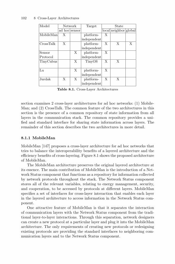
102 8 Cross-Layer Architectures
Model Network Target Statead hoc sensor local neighbor global
MobileMan X platform- Xindependent
CrossTalk X platform- X X Xindependent
Sensor X platform- XProtocol independent
TinyCubus X TinyOS X X
Lu X platform- Xindependent
Jurdak X X platform- X Xindependent
Table 8.1. Cross-Layer Architectures
section examines 2 cross-layer architectures for ad hoc networks: (1) Mobile-Man; and (2) CrossTalk. The common feature of the two architectures in thissection is the presence of a common repository of state information from alllayers in the communication stack. The common repository provides a uni-fied and standard interface for sharing state information across layers. Theremainder of this section describes the two architectures in more detail.
8.1.1 MobileMan
MobileMan [147] proposes a cross-layer architecture for ad hoc networks thattries to balance the interoperability benefits of a layered architecture and theefficiency benefits of cross-layering. Figure 8.1 shows the proposed architectureof MobileMan.
The MobileMan architecture preserves the original layered architecture atits essence. The main contribution of MobileMan is the introduction of a Net-work Status component that functions as a repository for information collectedby network protocols throughout the stack. The Network Status componentstores all of the relevant variables, relating to energy management, security,and cooperation, to be accessed by protocols at different layers. MobileManspecifies a set of interfaces for cross-layer interaction that enables each layerin the layered architecture to access information in the Network Status com-ponent.
One attractive feature of MobileMan is that it separates the interactionof communication layers with the Network Status component from the tradi-tional layer-to-layer interactions. Through this separation, network designerscan create a new protocol at a particular layer and plug it into the MobileManarchitecture. The only requirements of creating new protocols or redesigningexisting protocols are providing the standard interfaces to neighboring com-munication layers and to the Network Status component.
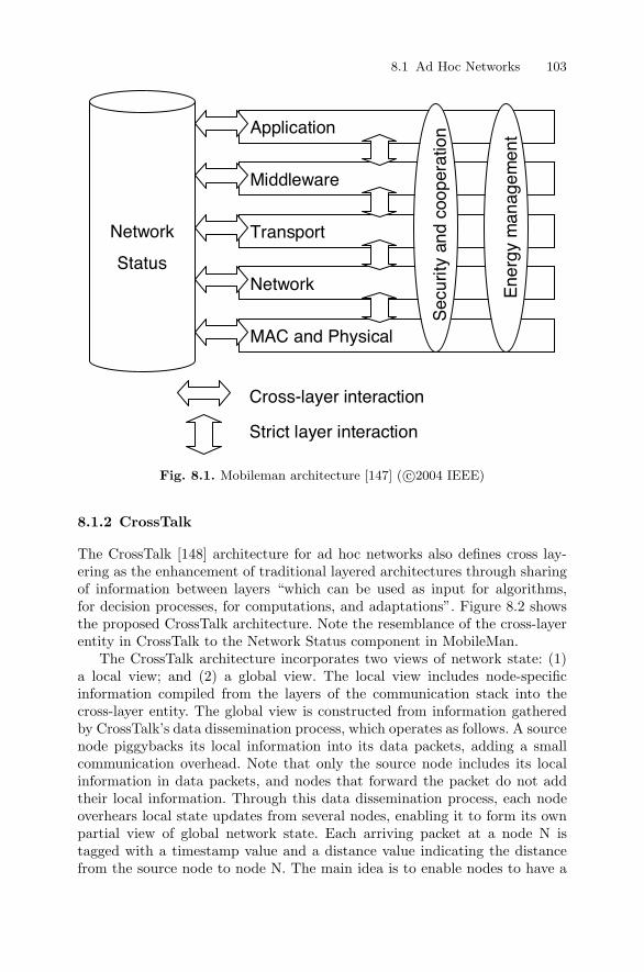
8.1 Ad Hoc Networks 103
Application
Middleware
Transport
Network
MAC and Physical
Network
Status
Sec
urity
and
coo
pera
tion
Ene
rgy
man
agem
ent
Cross-layer interaction
Strict layer interaction
Fig. 8.1. Mobileman architecture [147] ( c©2004 IEEE)
8.1.2 CrossTalk
The CrossTalk [148] architecture for ad hoc networks also defines cross lay-ering as the enhancement of traditional layered architectures through sharingof information between layers “which can be used as input for algorithms,for decision processes, for computations, and adaptations”. Figure 8.2 showsthe proposed CrossTalk architecture. Note the resemblance of the cross-layerentity in CrossTalk to the Network Status component in MobileMan.
The CrossTalk architecture incorporates two views of network state: (1)a local view; and (2) a global view. The local view includes node-specificinformation compiled from the layers of the communication stack into thecross-layer entity. The global view is constructed from information gatheredby CrossTalk’s data dissemination process, which operates as follows. A sourcenode piggybacks its local information into its data packets, adding a smallcommunication overhead. Note that only the source node includes its localinformation in data packets, and nodes that forward the packet do not addtheir local information. Through this data dissemination process, each nodeoverhears local state updates from several nodes, enabling it to form its ownpartial view of global network state. Each arriving packet at a node N istagged with a timestamp value and a distance value indicating the distancefrom the source node to node N. The main idea is to enable nodes to have a
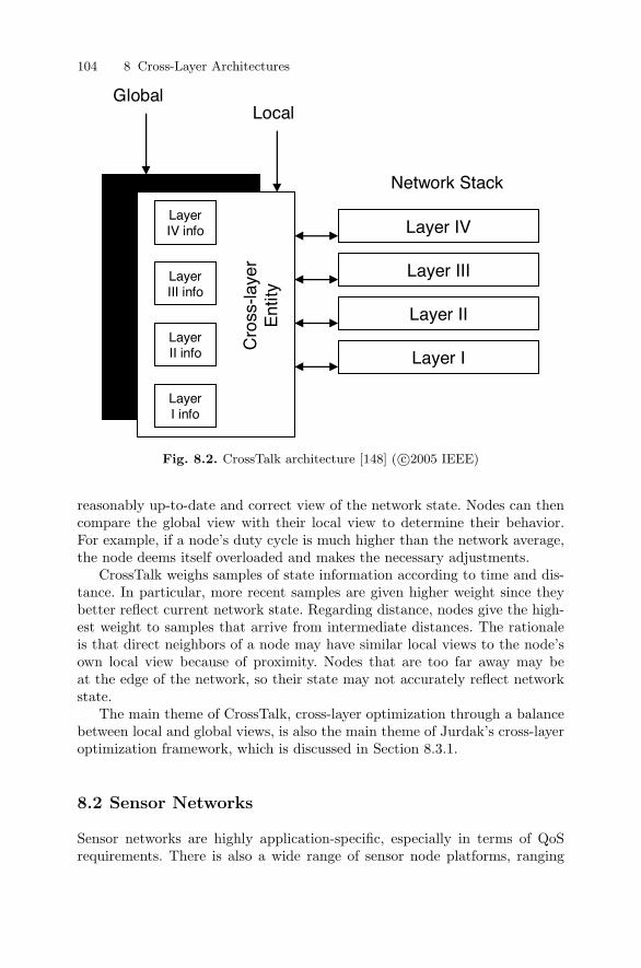
104 8 Cross-Layer Architectures
Layer IV
Layer III
Layer II
Layer I
Cro
ss-la
yer
Ent
ity
LocalGlobal
Network Stack
Layer I info
Layer II info
Layer III info
Layer IV info
Fig. 8.2. CrossTalk architecture [148] ( c©2005 IEEE)
reasonably up-to-date and correct view of the network state. Nodes can thencompare the global view with their local view to determine their behavior.For example, if a node’s duty cycle is much higher than the network average,the node deems itself overloaded and makes the necessary adjustments.
CrossTalk weighs samples of state information according to time and dis-tance. In particular, more recent samples are given higher weight since theybetter reflect current network state. Regarding distance, nodes give the high-est weight to samples that arrive from intermediate distances. The rationaleis that direct neighbors of a node may have similar local views to the node’sown local view because of proximity. Nodes that are too far away may beat the edge of the network, so their state may not accurately reflect networkstate.
The main theme of CrossTalk, cross-layer optimization through a balancebetween local and global views, is also the main theme of Jurdak’s cross-layeroptimization framework, which is discussed in Section 8.3.1.
8.2 Sensor Networks
Sensor networks are highly application-specific, especially in terms of QoSrequirements. There is also a wide range of sensor node platforms, ranging
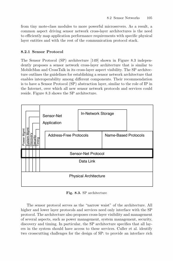
8.2 Sensor Networks 105
from tiny mote-class modules to more powerful microservers. As a result, acommon aspect driving sensor network cross-layer architectures is the needto efficiently map application performance requirements with specific physicallayer entities and with the rest of the communication protocol stack.
8.2.1 Sensor Protocol
The Sensor Protocol (SP) architecture [149] shown in Figure 8.3 indepen-dently proposes a sensor network cross-layer architecture that is similar toMobileMan and CrossTalk in its cross-layer aspect visibility. The SP architec-ture outlines the guidelines for establishing a sensor network architecture thatenables interoperability among different components. Their recommendationis to have a Sensor Protocol (SP) abstraction layer, similar to the role of IP inthe Internet, over which all new sensor network protocols and services couldreside. Figure 8.3 shows the SP architecture.
Sys
tem
Mgm
t
Data Link
Sensor-Net
Application
Address-Free Protocols Name-Based Protocols
Physical Architecture
In-Network Storage
Tim
ing
Sec
urity
Dis
cove
ry
Pow
er M
gmt
Sensor-Net Protocol
Fig. 8.3. SP architecture
The sensor protocol serves as the “narrow waist” of the architecture. Allhigher and lower layer protocols and services need only interface with the SPprotocol. The architecture also proposes cross-layer visibility and managementof several aspects, such as power management, system management, security,discovery and timing. In particular, the SP architecture specifies that all lay-ers in the system should have access to these services. Culler et al. identifytwo crosscutting challenges for the design of SP: to provide an interface rich
106 8 Cross-Layer Architectures
enough for application/SP collaboration, and to keep that interface platformindependent. The former challenge stems from the need for customized per-formance for each application, while the latter challenge stems from the widerange of sensor platforms available.
To address these two challenges, the SP architecture proposes having plat-form independent power management interfaces that are customizable to thedetails and tradeoffs of specific platforms. The SP architecture also providesa rich two-way interface between SP and the other protocols. These inter-faces enable the SP layer to share its information with other layers, and italso enables other protocols to share information with SP so that it can makesystem-wide resource management decisions.
8.2.2 TinyCubus
The TinyCubus [150] is a cross-layer framework for sensor networks basedon TinyOS that aims at providing a flexible and adaptive infrastructure foroptimizing sensor network applications with diverse performance goals. Fig-ure 8.4 shows the main components of the TinyCubus architecture, whichapproaches cross-layer optimization with a programmatic and implementa-tion perspective.
The TinyCubus architecture defines the Tiny cross-layer framework thatprovides interfaces to support information sharing among layers and to en-able lower layers to invoke application-specific code. To support cross-layerinformation sharing, the framework employs a state repository that stores allrelevant parameters for cross-layer access. To enable components to access thestate repository, the model defines a specification language that is responsiblefor generating interfaces to connect components with the shared data. Theinvocation of application-specific code by lower layers (also referred to as call-back) is achieved through an extension of existing TinyOS component wiringmechanisms.
Another component of the TinyCubus architecture is the Tiny Configura-tion Engine. The Configuration Engine includes a topology manager responsi-ble for network self-organization and for assigning a role to each node, such asSOURCE, AGGREGATOR, SINK or CLUSTER HEAD. The ConfigurationEngine also enables code distribution through the network for reprogrammingthe nodes in-situ.
The final component of the TinyCubus architecture is the Data Manage-ment Framework, which provides a standard set of data management andsystem components and chooses the best component set based on three di-mensions: system parameters, application requirements, and optimization pa-rameters. The system parameters refer to factors such as sensor density, noderesources, or mobility. The application requirements dimension refers to qual-ity of service metrics such as reliability or delay. Finally, the optimizationparameters determine the selected algorithm for the given constraints at thethree dimensions.
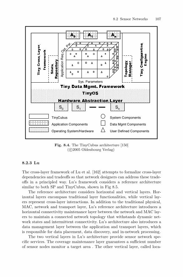
8.2 Sensor Networks 107
S0 S1 Sn
Sys. Parameters
TinyCubus
Application Components
Operating System/Hardware
System Components
Data Mgmt Components
User Defined Components
App
licat
ion
Req
.Opt
. Par
.
Fig. 8.4. The TinyCubus architecture [150]( c©2005 Oldenbourg Verlag)
8.2.3 Lu
The cross-layer framework of Lu et al. [162] attempts to formalize cross-layerdependencies and tradeoffs so that network designers can address these trade-offs in a principled way. Lu’s framework considers a reference architecturesimilar to both SP and TinyCubus, shown in Fig 8.5.
The reference architecture considers horizontal and vertical layers. Hor-izontal layers encompass traditional layer functionalities, while vertical lay-ers represent cross-layer interactions. In addition to the traditional physical,MAC, network and transport layer, Lu’s reference architecture introduces ahorizontal connectivity maintenance layer between the network and MAC lay-ers to maintain a connected network topology that withstands dynamic net-work states and intermittent connectivity. Lu’s architecture also introduces adata management layer between the application and transport layers, whichis responsible for data placement, data discovery, and in-network processing.
The two vertical layers in Lu’s architecture provide sensor network spe-cific services. The coverage maintenance layer guarantees a sufficient numberof sensor nodes monitor a target area . The other vertical layer, called loca-
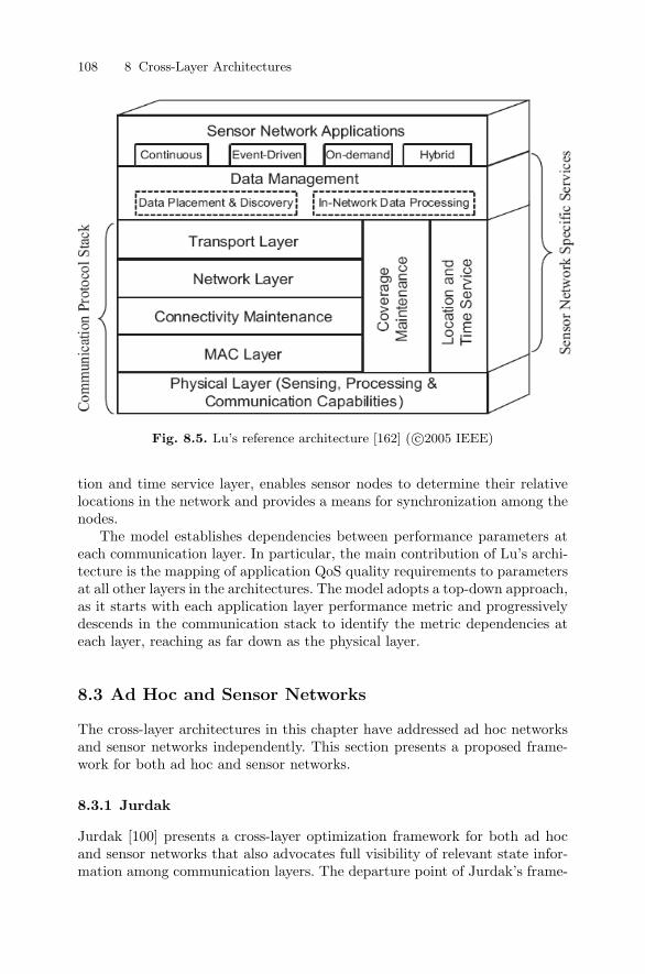
108 8 Cross-Layer Architectures
Fig. 8.5. Lu’s reference architecture [162] ( c©2005 IEEE)
tion and time service layer, enables sensor nodes to determine their relativelocations in the network and provides a means for synchronization among thenodes.
The model establishes dependencies between performance parameters ateach communication layer. In particular, the main contribution of Lu’s archi-tecture is the mapping of application QoS quality requirements to parametersat all other layers in the architectures. The model adopts a top-down approach,as it starts with each application layer performance metric and progressivelydescends in the communication stack to identify the metric dependencies ateach layer, reaching as far down as the physical layer.
8.3 Ad Hoc and Sensor Networks
The cross-layer architectures in this chapter have addressed ad hoc networksand sensor networks independently. This section presents a proposed frame-work for both ad hoc and sensor networks.
8.3.1 Jurdak
Jurdak [100] presents a cross-layer optimization framework for both ad hocand sensor networks that also advocates full visibility of relevant state infor-mation among communication layers. The departure point of Jurdak’s frame-
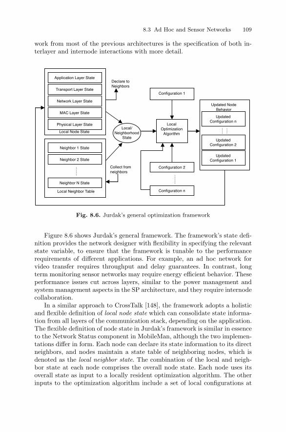
8.3 Ad Hoc and Sensor Networks 109
work from most of the previous architectures is the specification of both in-terlayer and internode interactions with more detail.
Application Layer State
Network Layer State
Physical Layer State
Neighbor 1 State
Neighbor 2 State
Neighbor N State
Local Node State
.……
Local Neighbor Table
Collect from neighbors
Local/ Neighborhood
State
Declare to Neighbors
Local Optimization
Algorithm
Configuration 1
Updated Configuration n
Updated Configuration 2
Updated Node Behavior
Configuration 2
Updated Configuration 1
Transport Layer State
MAC Layer State
.……
Configuration n
.….
..…
Fig. 8.6. Jurdak’s general optimization framework
Figure 8.6 shows Jurdak’s general framework. The framework’s state defi-nition provides the network designer with flexibility in specifying the relevantstate variable, to ensure that the framework is tunable to the performancerequirements of different applications. For example, an ad hoc network forvideo transfer requires throughput and delay guarantees. In contrast, longterm monitoring sensor networks may require energy efficient behavior. Theseperformance issues cut across layers, similar to the power management andsystem management aspects in the SP architecture, and they require internodecollaboration.
In a similar approach to CrossTalk [148], the framework adopts a holisticand flexible definition of local node state which can consolidate state informa-tion from all layers of the communication stack, depending on the application.The flexible definition of node state in Jurdak’s framework is similar in essenceto the Network Status component in MobileMan, although the two implemen-tations differ in form. Each node can declare its state information to its directneighbors, and nodes maintain a state table of neighboring nodes, which isdenoted as the local neighbor state. The combination of the local and neigh-bor state at each node comprises the overall node state. Each node uses itsoverall state as input to a locally resident optimization algorithm. The otherinputs to the optimization algorithm include a set of local configurations at

110 8 Cross-Layer Architectures
the node. The local optimization algorithm determines the resulting node be-havior consisting of the updated configuration set. The updated configurationmay result in changes to the local node state. The strength of Jurdak’s ap-proach is its validation for three different case studies of ad hoc and sensornetworks, which we present in detail in Part III of the book.
9
Applied Cross-Layer Approaches
The previous two chapters have presented cross-layer design and architecturalissues for ad hoc and sensor networks. This chapter focuses on the appliedcross-layer approaches for ad hoc and sensor networks.
Applied cross-layer approaches for ad hoc and sensor networks fall intotwo broad categories: design coupling approaches and information sharing ap-proaches. Design coupling approaches ignore layer boundaries to propose al-gorithms that optimize network performance metrics by integrating function-alities from different layers. Information sharing approaches attempt to shareinformation across layers while maintaining architectural protocol boundaries.
Based on our survey of existing approaches, we extract 5 characterizingfeatures of applied cross-layer approaches for ad hoc and sensor networks:(1) global performance goals; (2) target networks; (3) independent optimiza-tion variables; (4) dependent optimization variables; and (5) implementationdesign. The first feature, global performance goals, deals with the desired per-formance improvement of the cross-layer model on a global or network-widescale. Next, the target networks feature specifies the class of networks forwhich a cross-layer model is customized. The third feature, independent op-timization variables, includes one or more variables that serve as the inputof a cross-layer model. Supporting the cross-layer nature of the models inthis chapter, the independent variables may provide state information fromseveral layers across the network stack. The model can then use the indepen-dent variables for determining how to optimize node configurations, whichleads us to our fourth feature. A model’s dependent optimization variablesrepresent the output set of variables from across the communication stack.In other words, the model determines the dependent optimization variablesbased on the synthesis of the independent variables and the current config-uration to determine optimal network behavior. Our final feature deals witha models’ proposed implementation approach. Some models are algorithmicin nature, while others explicitly specify the internode collaboration strategyand the locale of required computation. Centralized models collect networkstate information at a central controller that runs comprehensive optimiza-
112 9 Applied Cross-Layer Approaches
tion algorithms, while distributed models spread the required computation forcross-layer optimization across several nodes.
Before classifying the cross-layer approaches according to the manner inwhich they address each feature in the subsequent sections, the next two sec-tions provide an overview of the operation of each cross-layer approach. Sec-tion 9.1 discusses the optimization approaches that rely on design coupling.Section 9.2 presents cross-layer approaches that focus on information sharingwithin an architectural preserving framework. The remaining sections com-pare the applied approaches according to the 5 characterizing features. Sec-tion 9.3 surveys and compares the different performance goals of applied cross-layer approaches. Section 9.4 classifies the cross-layer approaches according totheir target networks. Section 9.5 discusses the independent optimization vari-ables considered in the existing approaches, and Section 9.6 reveals how eachmodel uses the independent variables for determining optimal configurations.Section 9.7 focuses on the practical and architectural implementation issuesof each model in distributed ad hoc and sensor networks.
9.1 Design Coupling Approaches
Cross-layer approaches that rely on design coupling of adjacent layers disre-gard layer boundaries and treat network mechanism as a single algorithmicblock that optimizes certain performance metrics. The combinatorial aspectof these approaches typically yields a lack of specification of the functional orarchitectural issues, focusing mostly on algorithmic design.
Table 9.1 provides an overview of the features of existing cross-layer ap-proaches for ad hoc and sensor networks that rely on design coupling. Thecolumns in Table 9.1 correspond to the 5 features, while the rows correspondto existing approaches. Sections 9.3 through 9.7 will revisit the classificationin Table 9.1 with more detail.
9.1.1 Girici and Ephremides
Girici and Ephremides [158] propose a cross-layer approach based on jointrouting and link scheduling for ad hoc networks. Their approach aims atmaking routing and link activation decisions that are aware of three aspects:energy, delay, and network lifetime. To enable aspect-aware decisions, thenodes store the state of neighboring nodes, including residual battery energy,available number of transceivers, and transmission power requirements of eachneighbor.
The purpose of this approach is to solve the following energy efficientrouting problem: to enable a node to select the best next hop for each packetaccording to energy, delay, and network lifetime considerations. For this pur-pose, Girici and Ephremides’s approach introduces a new link cost metric thatconsiders three terms: transmission energy per packet (physical layer aspect),

9.1 Design Coupling Approaches 113
Model
Goals
Targ
etIn
put
Asp
ects
Opti
miz
ati
ons
Des
ign
12
3N
etw
ork
Net
work
Data
Lin
kP
hysi
cal
Tra
nsp
ort
Net
work
Data
Lin
kP
hysi
cal
Gir
ici
net
work
min
imum
ener
gy
TD
MA
queu
elink
trans.
route
link
unsp
ecifi
ed[1
58]
life
del
ayeffi
cien
cyad
hoc
length
thro
ugh-
pow
erco
stsc
hed
ule
net
work
sput
uti
liza
tion
Cru
zen
ergy
wir
eles
sav
erage
maxim
um
route
link
trans.
dis
trib
ute
d[1
59]
effici
ency
base
link
trans.
cost
sched
ule
pow
erst
ati
ons
rate
pow
er
ElB
att
maxim
um
ener
gy
TD
MA
SN
Rlink
trans.
centr
alize
d[1
60]
thro
ugh-
effici
ency
CD
MA
inte
rfer
ence
sched
ule
pow
erput
ad
hoc
net
work
s
Koza
ten
ergy
TD
MA
link
BE
Rlink
trans.
centr
alize
d[1
61]
effici
ency
ad
hoc
rate
sSN
Rsc
hed
ule
pow
ernet
work
s
Lu
maxim
um
min
imum
ener
gy
TD
MA
SN
Rlink
trans.
unsp
ecifi
ed[1
62]
thro
ugh-
del
ayeffi
cien
cyse
nso
rsc
hed
ule
pow
erput
net
work
s
Madan
net
work
TD
MA
route
SN
Rlink
trans.
unsp
ecifi
ed[1
63]
life
senso
rflow
sched
ule
rate
net
work
spow
er
Wang
maxim
um
fair
ad
hoc
link
sess
ion
link
dis
trib
ute
d[1
66]
thro
ugh-
acc
ess
net
work
sra
tera
tes
att
empt
put
pro
bability
Cui
ener
gy
TD
MA
pro
cess
ing/
route
link
MQ
AM
unsp
ecifi
ed[1
64]
effici
ency
senso
rtr
ans.
cost
sched
ule
trans.
net
work
spow
er
Mer
zm
axim
um
UW
BT
H-c
ode
tim
ers
code
dis
trib
ute
d[1
72]
thro
ugh-
ad
hoc
rate
put
net
work
s
Table
9.1
.A
pplied
Cro
ssLay
erA
ppro
ach
esbase
don
Des
ign
Coupling
114 9 Applied Cross-Layer Approaches
expected volume on a node’s links throughout the network lifetime (datalink layer aspect), and the queue length along the directed link (network layeraspect). The link metric definition provides a tunable coefficient for each termin order to favor any of the three terms.
This approach adopts a slotted time structure with a separate time-slottedcontrol channel that enables nodes to reserve slots for data delivery. Each timeslot is subdivided into a request and a confirm slot. In order to request a timeslot, a node issues a REQUEST message, to which the receiver replies with aCONFIRM message. Upon receiving the CONFIRM message, the sender canproceed with data transmission in the reserved time slot.
Girici and Ephremides’s approach attempts to schedule links by consider-ing communication performance as a utility and assign each link a dynamicallychanging utility value, according to a predefined link activation utility metric.The ultimate goal is maximizing the sum of the utility values of the links inthe resultant set of scheduled links.
The new link utility metric encourages the activation of congested links,and it discourages activation of links with high-energy destination nodes.Through this mechanism, the queue sizes of the highly congested links re-main large and they are not preferred in routing, which prevents those nodesfrom early death. The new metric also encourages activation of links requiringlow RF power, so that their queue sizes remain low and they are preferred forrouting.
The performance evaluation of this approach through simulations to inves-tigate the effect of each term the in routing metric confirms that the averageenergy per packet in the network is minimized when the routing metric onlyincludes the transmission energy per link. Expanding the routing metric toinclude delay or lifetime metrics causes higher transmission energy per packet.Another intuitive result is that delay performance is best when queue sizesare included as part of the routing metric. Finally, including the node residualenergies into the routing metric enables more load balancing in the networkand it prolongs the time at which the first node in the network dies.
Acknowledging the inherent tradeoff between energy, delay, and deliveredtraffic, the results of Girici and Ephremides’s study confirm that link metric-based policies that jointly considers transmission power requirements, resid-ual energy information, link queue sizes and transceiver utilization providesa balance in terms of energy consumption, average delay and delivered traf-fic volume. This work is one of the first to address the joint power and linkscheduling problem. However, the algorithmic nature and the lack of any in-terlayer interaction specification limit the approach’s applicability to existingarchitectures. Furthermore, this optimization approach does not specify howto run the required computation in distributed networks, leaving several openissues regarding its implementation in real networks.
9.1 Design Coupling Approaches 115
9.1.2 Cruz and Santhanam
Cruz and Santhanam [159] present a cross-layer approach with the expandedgoals of joint routing, link scheduling, and power control among a networkof wireless base stations. Although their approach does not focus on purelyad hoc networks, the cross-layer design concepts in this approach are readilyapplicable to ad hoc and sensor networks. The main goal for Cruz and San-thanam’s approach is to minimize the total average transmission power in thenetwork subject to constraints regarding the minimum average data rate perlink and the peak transmission power.
The approach requires synchronization to support its time-slotted struc-ture, and it assumes that the interference conditions do not experience anysmall time-scale variations. Cruz and Santhanam identify the tradeoff ofscheduling wireless links that are far apart to minimize interference and ofscheduling links closely to achieve high data rates in the network. As such,Cruz and Santhanam’s approach tries to systematically optimize the activesubsets of links in the network and their respective transmission powers inorder to minimize the total average power expended in the network. The op-timal link schedules are also constrained by a minimum data rate and a peaktransmission power for each node. The derivation of their optimal policy re-veals that each node should either turn off its transceiver or transmit at themaximum allowable transmission power. In order to reduce their algorithm’scomplexity, they also limit the search space of the optimal schedule by onlyconsidering feasible links.
The computational cost for a group of more than 15 links grows quickly,limiting the scalability of this approach. To support larger networks, the au-thors suggest a hierarchical clustered approach in which each cluster has atmost 15 links. The clusters are considered to schedule links independently ofeach other.
After determining optimal link and power schedules, Cruz and San-thanam’s approach takes on the problem of allocating traffic on the scheduledlinks to support a given traffic matrix describing the required traffic rates ofspecific source destination pairs. The approach uses a shortest path routingalgorithm to incrementally compute the cost of supporting additional trafficon each link, and uses an iterative approach which eventually converges toan optimal route assignment. The optimal routing paths for traffic purposesdo not always correspond to minimum energy paths. However, their routingpolicy uses minimum energy paths whenever the data traffic requirements arelow.
At low traffic loads, Cruz and Santhanam’s approach reduces to a simpleTDMA policy that activates one link at a time in sequence. At higher trafficloads, the approach supports higher data rates than TDMA through con-current scheduling of links. The cost of higher throughput is reduced energyefficiency, since more nodes and links are involved in the concurrent transmis-sions. For example, forwarding data along multiple paths may provide higher

116 9 Applied Cross-Layer Approaches
throughput, but it involves more forwarding activity at intermediate nodeswhich translates into higher power consumption.
Cruz and Santhanam’s approach is general enough to apply to clusteredtopology ad hoc and sensor networks despite the fact that it develops theoptimization approach for a network of wireless base stations. Some of thelimiting assumptions of this approach include synchronized node clocks andslow varying interference conditions. Another inherent drawback to this al-gorithmic approach is the lack of implementation or functional description.It also uses a performance metric of long term rate requirement, meaningoptimal solutions may involve significant rate fluctuations.
9.1.3 ElBatt and Ephremides
In a similar approach, ElBatt and Ephremides [160] try to optimize the jointpower control and TDMA scheduling problem. The distinction of this ap-proach is that it specifically targets contention-based wireless ad hoc networks,whereas Cruz and Santhanam’s approach targets wireless base stations. Elbattand Ephremides’s approach consists of 2 phases:
1. link scheduling: The scheduling phase coordinates the transmissions ofindependent users in order to eliminate strong levels of interference.
2. power control: The power control phase runs in a distributed fashion todetermine the admissible power vector to be used by scheduled users tosatisfy their single-hop transmission requirements.
The mechanisms of this approach attempt to adapt existing TDMA andCDMA cellular network mechanisms for ad hoc networks through cross-layerenhancements. Elbatt and Ephremides develop their model based on severalassumptions, of which the following are most notable:
• There is a central controller that runs the scheduling algorithms• Nodes exchange short control messages through a separate contention-free
control channel• Nodes are aware of the locations of all other nodes in the network• In addition to interference of neighbor communications, nodes that are
further away also cause interference according to a realistic interferencemodel
This approach does not consider mobility or routing aspects. It exploitsthe notion of spatial channel reuse for nodes that are separated by a distancelarger than a computed channel reuse distance.
The approach splits the optimization problems into 2 separate optimiza-tion problems. The first optimization problem is the “valid scenario optimiza-tion” problem: to find the valid set of nodes, which is the largest subset ofnetwork nodes that can simultaneously transmit packets. The second opti-mization problem is the “admissible scenario” problem, which determines the
9.1 Design Coupling Approaches 117
largest subset of the valid set that can satisfy the SNR constraints of all theactive links.
Elbatt and Ephermides propose a distributed power control algorithmmodeled after cellular networks. They prove through analysis and simulationsthat the computation complexity of their algorithm for valid transmissions inboth TDMA and TDMA/CDMA wireless ad hoc networks grows exponen-tially with the number of links. Their simulations also reveal that CDMA sys-tems provide higher single-hop throughput and lower transmission power thanTDMA systems, at the cost of higher processing power. Elbatt and Epher-mides’s cross-layer optimizations also significantly increase the throughputand decrease the transmission power cost over the heuristic case, especiallyunder heavy load conditions.
One advantage of this approach is that it builds on previous cellular net-work concepts, such as spatial reuse of resources. Unlike previous algorithmsthat do not address computational distribution, this approach is that it ad-dresses the computation distribution issue, and it theoretically shows thatcomputation can be distributed across the nodes. However, it does not specifyhow to practically achieve the computational distribution. Multihop routingand mobility are two other issues not addressed in this approach. Finally, theassumption that all nodes are location-aware introduces cost and complexityto this approach.
9.1.4 Kozat
Kozat et al. [161] propose another cross-layer approach that attempts to min-imize power consumption in an ad hoc network while providing quality of ser-vice guarantees in terms of bandwidth and bit error rate. As in [159] and [160],this approach involves collaboration between the MAC and physical layers.Because Elbatt and Ephermides’s approach is inspired by cellular networks, itdoes not address multihop cases. Kozat’s approach extends the single hop con-siderations of Elbatt’s approach to handle multihop networks. Kozat’s maindistinction from Cruz’s approach is that Kozat’s approach addresses the short-term throughput, where Cruz’s approach focuses on the long-term averagethroughput. Because obtaining the optimal solution is NP-hard, Kozat et al.propose heuristics for link scheduling and power control with quality-of-serviceguarantees.
Kozat’s approach assumes that there are a number of sessions activethrough the network, and that each session is predetermined through somerouting protocol. Each session consists of a source-destination pair, a set ofdirected links from source to destination, a short-term end-to-end bit rate,and a per-link bit error rate. This approach assumes that time is divided intoslots, and that the scheduling algorithm must assign one or more slots pertransmitter during each time frame.
This model also provides a one-to-one mapping between the modulationlevel, bit error rate and the signal to noise ratio. Because the model assumes
118 9 Applied Cross-Layer Approaches
that the coding rate and modulation level are kept fixed throughout the frame,it relies on transmit power control and slot assignment for satisfying the biterror rates as the interference level varies with time.
Kozat’s approach introduces the concept of virtual links. In certain net-works, separate sessions may use the same link for forwarding data. Eachinstance of the same link that appears on multiple paths is indexed separatelyand is denoted as a virtual link. As such, several virtual links may correspondto the same physical link.
Although the central aim of this approach is to minimize the total transmitpower as summed over all time slots and links while satisfying the minimumrate and SINR constraints of the sessions, Kozat et al. analytically reducethis problem to a classical power control problem in cellular networks oncea particular slot is allocated. As a result, they propose two algorithms forsolving these optimization problems.
The first algorithm adopts a top-down approach. The algorithm beginswith a set of empty time slots in a frame and a set of unscheduled virtuallinks. The algorithm starts with the first time slot and attempts to fill thatslot with as many virtual links as possible. Because this approach assumes halfduplex point-to-point communication, virtual links scheduled during the sameslot must not have any transmitters or receivers in common. The algorithmthen checks if there is a feasible power allocation for the set of scheduledvirtual links. In case the allocation is not feasible, high interference linksare pruned from the allocation until the power allocation becomes feasible.The two phases in this algorithm resemble Elbatt and Ephermides’s 2 phasesolution for the link scheduling and power allocation problem.
The second algorithm adopts a bottom-up approach, by performing theiteration over the unassigned links. This algorithm initially assigns exactlyone link to each slot until all slots have exactly one link. It always chooses thelink with the maximum interference among all the unassigned links to placein the next empty slot. This ensures that transmitters that are within closerange of each other are spread onto different time slots. The second stage ofthis algorithm adopts a water-filling approach. A link is assigned to a slot ifthis assignment is feasible and if the slot has an acceptable power allocationafter this new link assignment. This algorithm completes when all links havebeen checked or when it is not possible to place new links in any of the slots.
The performance evaluation of this approach through simulations thatconsider minimum hop routing and minimum power routing reveals that thetop-down design strategy (which entails first solving the feasibility problem,then minimizing the power consumption) performs better in terms of theobjective cost function. The second algorithm which adopts a bottom-up ap-proach (water-filling) performs better than the top-down design strategy infinding a feasible solution for link scheduling and power allocations.
Regarding the interaction with the routing strategy, Kozat et al. notethat including power considerations at the routing layer plays a dominantrole in reducing power consumption, but it also may adversely affect QoS
9.1 Design Coupling Approaches 119
guarantees at the data link and physical layers. As in previous approaches,Kozat’s approach lacks mobility support, because it considers that link gainsremain constant within a time frame.
This approach adopts an open view towards including more layer function-alities, although it focuses on scheduling and power control at the data linkand physical layers respectively. This framework’s support for integration ofhigher layer functionalities, such as QoS metrics, contributes to its flexibility.Other strengths of this approach include the realistic assumption of short-term link quality variations, and the introduction of the concept of virtuallinks. The algorithmic nature of this approach is a limiting factor towards itsimplementation, especially the centralized computation structure that con-siders that the input data for the algorithm can be compiled at one location.Finally, this approach optimizes link schedules and transmission powers basedon the assumption that routes are already established. In practical scenarios,this assumption is simplistic since routing issues are closely intertwined withlink scheduling and power control issues.
9.1.5 Lu and Krishnamachari
Lu and Krishnamachari [162] attempt to extend earlier work on the jointscheduling and power control problem by proposing a tunable framework thatmanages the tradeoffs between throughput, energy and latency. This approachnotes that previous works on joint scheduling and power control [160] attemptto pack the maximum number of links that can be active simultaneously ineach time slot. Although the power control phase minimizes the transmissionpowers on the scheduled links, this scheduling policy does not take energy intoconsideration and thus may not be energy efficient. Through parametrizationof the performance aspects, Lu’s approach achieves significant energy savingswithout sufficiently sacrificing throughput.
Lu and Krishnamachari’s approach makes the following assumptions:
• It operates in a static sensor network where all nodes have omnidirectionalantennas
• It considers a periodic data gathering application in which nodes sendtheir packets to a sink or to neighbors with a delay bound
• It supports applications with per-hop or end-to-end deadlines. In the lattercase, the approach computes per-hop deadlines by dividing end-to-enddeadlines by the number of hops along a path
• It assumes a TDMA multiple access strategy• Each node generates a random amount of packets during a time frame• It considers the packets to be forwarded at a node as local transmission
requests
Lu and Krishnamachari’s approach also exploits a more realistic SNRmodel. Within this model, links can be scheduled concurrently in the sametime slot if their SNR values are larger than a certain threshold. The SNR
120 9 Applied Cross-Layer Approaches
is computed as the ratio of the received signal power to the sum of the noiseand the interference of all other concurrent links.
To promote flexibility, Lu and Krishnamachari’s approach defines a tun-able gain function. The total gain in the network is the weighted difference ofthe throughput and the energy cost. To simplify the analysis, the weight of thethroughput can be fixed to 1 in order to focus the optimization on choosingthe weight of the energy cost to serve different applications. For applicationsthat favor energy efficiency, the energy cost has a weight larger than 1. Incontrast, applications with high throughput requirement can set a weight forthe energy cost that is smaller than 1. The optimization problem is subjectto worst case per-hop delay constraints.
When the energy cost weight is set to zero, Lu and Krishnamachari’s prob-lem reduces to the same problem in [160]. For the more general optimizationproblem, several heuristics are proposed.
The first greedy algorithm assumes that the collection of all feasible trans-mission sets S is given, and this algorithm selects the appropriate link sets tobe scheduled in the same time slot by iteratively choosing the next set thatmaximizes the total gain. The computational complexity of this algorithmgrows exponentially with the number of links, making it suitable for smallclusters in large sensor networks.
The second heuristic introduces two new assumptions: (1) that link gainschange slowly during a frame; and (2) that all nodes can stay informed of alllink gains. It also assumes that nodes exchange short control messages at thebeginning of every time frame to announce their links to be scheduled. Thisalgorithm then obtains all the feasible transmission scenarios for a time frameand compares the overall gain of each scenario, through the gain functionthat includes delay, throughput and energy to choose the scenario with thelargest gain. The computational complexity of the second heuristic also growsexponentially with the number of links.
The performance evaluation of this approach yields two main results. First,by relaxing the latency bound, the approach can achieve significant energysavings. Second, by varying the weight of the energy cost, the algorithm isable to save significant energy without hurting throughput.
The main advantage of this approach is the provision of a tunable frame-work for customizing network behavior to different application requirementsincluding throughput, delay, and energy. The assumptions for algorithm de-velopment are realistic and not limiting. The drawback of this approach is itsstrictly algorithmic nature and its lack of implementation details.
9.1.6 Madan
Madan et al. [163] propose another sensor network cross-layer optimizationapproach for sensor networks that aims at maximizing the network lifetime,defined as the time at which the first node dies in the network. In contrast
9.1 Design Coupling Approaches 121
to prior approaches that target energy efficiency, Madan’s approach specifi-cally addresses the key issue of network lifetime in sensor networks. Optimiza-tions for energy efficient behavior do not necessarily yield the longest networklifetime. For example, a strategy that minimizes overall power consumptionmay not balance traffic load, causing certain nodes to die earlier than others.Madan’s approach adjusts transmission rate, transmission power, link sched-ules, and routes in order to satisfy network lifetime constraints.
The approach advocates multihop routing and load balancing at the rout-ing layer. Multihop routing aims at replacing long communication links withmultiple short links to reduce transmission power consumption. Load bal-ancing aims at shifting traffic away from hot spots in the network for morebalanced energy consumption. As in the model in [160], Madan’s approachalso exploits spatial channel reuse for link scheduling.
As in most models discussed in this chapter, Madan’s approach targetsTDMA sensor networks. The approach also considers that each node gener-ates data at a fixed rate, which needs to be communicated to a single sinknode. Because the lifetime optimization problem is NP-hard, the problem canbe recast as a convex optimization problem by restricting links to TDMAschedules and by allowing variable length slots.
Madan’s optimization algorithm starts with a feasible suboptimal schedule.It computes the optimal transmission rates and powers for this schedule. Thealgorithm then checks if the schedule is feasible, in which case it disables linkswith SNR close to 1. It then allocates an additional time slot to a link with themaximum average power. This step repeats until it converges to the optimalsolution. At every iteration, the algorithm terminates in case of a repeatedschedule, unfeasible schedule, or unfeasible SNR. Checking these conditionsensures that the schedule at the end of each iteration is feasible.
To support partially distributed computation, Madan et. al reformulatethe problem to address the optimization of transmission powers and rates fora fixed link schedule. In particular, they show that each node can compute asubproblem of the complete optimization problem during each iteration. Ofcourse, distributed computation for this optimization must manage controlmessage exchanges for sharing schedule information, an issue which is notaddressed in Madan’s approach. Anther open issue for this approach is therealistic definition of network lifetime. Modeling sensor network lifetime re-quires a comprehensive approach that takes into account power consumptiondue to sensing, processing, communication, and switching hardware compo-nents between different power states.
The main advantage of this approach is its potential for distributed com-putation, although the mechanisms for distributed implementation are notclear. This approach’s performance goal to maximize sensor network lifetimeis also a highly practical issue in sensor networks. The drawbacks of this ap-proach include the purely algorithmic nature and the unrealistic definition ofnetwork lifetime.
122 9 Applied Cross-Layer Approaches
9.1.7 Cui
The same authors of Madan’s approach propose Cui’s cross-layer optimizationapproach [164] that targets energy efficiency in small scale sensor networks.What distinguishes Cui’s approach from previous approaches is that it con-siders both the communication power and the hardware power as the causesof power consumption in small scale sensor networks, partially addressingthe unrealistic power modeling of their previous approach. The argument isthat the hardware power consumption, which includes processing and sens-ing power consumption, may equal or even overweigh communication powerconsumption when communication links span short distances. Thus, Cui’sapproach considers both causes of power consumption to jointly determinecommunication paths, link schedules, M-ary Quadrature Amplitude Modula-tion (MQAM) modulation rates and transmit powers that yield better energyefficiency in the network.
This model assumes that the nodes maintain synchronization and oper-ate with a predetermined TDMA schedule. It also assumes that nodes arestationary or quasi-stationary, meaning that nodes may move at very slowspeeds. Furthermore, it considers that link schedules are interference-free andperiodic; once a node schedules its transmission during a particular time slotin a time frame, it uses the same time slot for its transmissions in subsequenttime frames.
Cui’s approach addresses a common sensor network topology, where allnodes send their data to a single sink node. In general, this approach requiresthat each node send its data toward a single destination. As in many peri-odic data gathering sensor network applications, data becomes available fortransmission periodically at each node.
Cui et al. use an energy model that considers two power states: active,and sleep. In the active mode, the node is either transmitting or receivingdata. During sleep periods, the node shuts off all of its circuitry. The powerconsumption due to leakage current and the transitional phase for switchingbetween active and sleep mode is neglected. This approach uses the circuitmodel from [165] for the transmit and receive signal paths. It also neglects theenergy consumption of baseband signal processing blocks, such as for sourcecoding, pulse-shaping, and digital modulation.
Finally, this approach explores energy-delay tradeoffs related to this cross-layer optimization problem. In particular, Cui et al. consider that queuingdelay and transmission delay are the sole contributors to packet delay at anode, thereby ignoring propagation delay which is negligible in small scalesensor networks. A notable observation is that in a TDMA tree topology,scheduling a node’s incoming links before its outgoing links on a particularpath minimizes packet delay. The validity of this claim can be seen by exam-ining the reverse case, where nodes schedule their outgoing links before theirincoming links. A node would send its packets from the last time frame alongits outgoing link, meaning the packet for this period would experience a delay
9.1 Design Coupling Approaches 123
equal to the time frame period. Packets would experience this delay at everyhop to the destination, yielding a relatively large end-to-end delay in multihopnetworks. The authors also show how to generalize the tree topology problemto a random graph topology.
One strength of this approach is the joint consideration of routes, linkschedules, transmission power, and modulation rates. Another novel contri-bution is the consideration of circuit power consumption in addition to trans-mission power consumption. However, this approach neglects other causes ofpower consumption, such as baseband signal processing blocks, leakage cur-rents and the transitional phase for switching between active and sleep mode.It is also a highly algorithmic approach that does not specify implementationdetails for mapping the algorithm to interlayer or internode interactions inexisting architectures. Finally, the predetermined TDMA schedule in this ap-proach is a limiting factor for sensor networks with dynamic data reportingconditions.
9.1.8 Wang and Kar
Wang and Kar address the rate control problem in multi-hop ad hoc networksin order to achieve proportional fairness among end-to-end sessions [166]. Inparticular, their approach considers the complex problem of maximizing thebandwidth utilization while maintaining fairness among active sessions. Ac-cording to Wang and Kar, the dependance of link rates on MAC parameterssuch as transmission probabilities or back-off window sizes necessitates jointoptimization at both the transport and data link layers. The main challenge isto specify the cooperation between the data link layer and the transport layerso that the aggregate utilities of all end-to-end sessions are maximized. Tosolve the joint optimization problem, Wang and Kar propose two algorithms:a dual-based algorithm, and a primal-based algorithm.
In the dual-based algorithm, active sessions adjust their rates in a dis-tributed manner in order to achieve fair session rates given a set of specificlink rates. The algorithm relies on iterative optimization between the linkand transport layers, albeit at different time scales. Each node periodicallyupdates the link rates (at the data link layer) using information collected fromthe local neighborhood on current link prices and link attempt probabilities.Whenever the link layer updates attempt probabilities, the transport layerbegins an iterative search for the optimal end-to-end session rates and opti-mal link prices (on the basis of the updated link rates). Thus, the transportlayer operates at a smaller time scale and the link layer operates at a largertime scale.
The primal-based algorithm transforms the non-convex joint optimizationproblem into a convex one through simple transformations. The main distinc-tion of the primal based algorithm is that the transport and data link layerswork at the same time scale. While the link layer updates link rates using
124 9 Applied Cross-Layer Approaches
the link attempt probabilities of neighboring nodes, the transport layer up-dates the session rates using aggregate traffic load and capacity information ofthe links on the active paths. Updating configurations in parallel at both thedata link and transport layers yields a faster convergence rate to the optimalsolution in comparison to the dual-based algorithm.
Both of the proposed algorithms attempt to optimize a logarithmic utilityfunction of the session rates. The choice of the logarithmic utility functionis well-suited for the target problem: the proportionally fair rate control op-timization problem. The difference between the two algorithms convenientlyillustrates some of the trade-offs of cross-layer design strategies. While bothalgorithms couple optimization at the transport and data link layers, thedual-based algorithm leans more towards information-sharing, maintainingmodularity between the transport and data link layers. Programmatically,the dual-based algorithm converges more slowly to the optimal solution sinceit involves embedded loops between the data link and transport layers. Thetransport layer iteratively works in the inner loop to optimize session ratesand link prices, while the data link layer works in the outer loop to adjust thelink attempt probabilities and link rates. The embedded loop structure causesa longer convergence time. In the primal-based algorithm, both the transportand the data link layer adjust their configuration according to the same timescale. As a result, the inter-layer interaction occurs at each iteration, whichenables faster convergence to the optimal configurations. The primal-based al-gorithm improves convergence time through a closer design-coupling betweenthe transport and data link layers.
The main advantage of Wang and Kar’s approach is the distributed natureof both algorithms. In particular, both algorithms rely on link information thatcan be collected locally at each node to optimize the utility function and topromote fairness. One drawback of this approach is its iterative nature, whichrisks intensive and ongoing computation in mobile or resource-limited nodes inad hoc and sensor networks. In the case of highly dynamic or mobile networks,the algorithm may initiate often, sometimes even before it reaches the optimalconfiguration for the previous epoch. Furthermore, this approach assumes asymmetric hearing matrix, which does not capture potential asymmetries ofunidirectional wireless links. Nonetheless, Wang and Kar’s approach demon-strates the benefits of cross-layer interaction between the transport and datalink layers.
9.1.9 Merz
Merz et al. take a step away from algorithmic design coupling toward a morefunctional approach in cross-layer design for ad hoc networks [172]. In partic-ular, their approach integrates functions from the physical and MAC layers inUWB ad hoc networks to maximize network throughput. It is worth notingthat the move from algorithmic to functional design required addressing amore specific network scenario that uses UWB technology.
9.2 Information Sharing Approaches 125
Merz’s approach considers the spread-spectrum nature of UWB networks,which separates concurrent transmissions on the same channel through time-hopping codes. The price for supporting multiple transmissions is that con-current transmissions cause mutual interference, which reduces link qualities.Reduced link qualities require either the increase of the transmission poweror the reduction of transmission rates. Since Merz’s approach aims at alwaysusing the maximum transmission power on all links, it proposes the dynamicadjustment of active link rates with the level of interference. The approachachieves rate adjustment through dynamic channel coding. The dynamic chan-nel coding algorithm employs incremental channel redundancy. A source nodesends the receiver packets with a high code rate. As long as the receiver cannotdecode the sender’s packet, the receiver sends negative ACKs (NACK) back tothe sender. Upon receiving NACKs, the sender lowers the code rate (increas-ing redundancy) and tries sending another packet with the lower rate. Thisprocess repeats until the sender receives an ACK message from the receiverindicating that it could decode the most recent packet. At that point, datatransmission proceeds with the highest possible code rate.
In addition to the handshake for code rate determination, Merz’s approachclosely couples the MAC layer functionality with the underlying UWB phys-ical layer. The MAC protocol adopts receiver-specific time-hopping codes. Asender always uses the intended receiver’s code for transmissions. After send-ing a data packet, a source node listens on the receiver’s TH-code for anACK message. Once it receives the ACK, the sender listens on its own TH-code again. Merz et al. also specify signalling procedures for indicating idlechannels, deferring transmissions, back-off timers, and failed transmissions.
The advantages of this approach include its support for distributed compu-tation and its specification of the relevant node interactions. Another strengthis the introduction of interference mitigation as an alternative to mutual exclu-sion in UWB networks. The main disadvantage of this approach is that it doesnot support rate guarantees for real-time applications, since the transmissionrate is always dependent on interference.
9.2 Information Sharing Approaches
Information sharing approaches preserve the existing layer functionality of areference architecture while providing novel means for interlayer interaction,in attempt to balance generality and performance. Information sharing ap-proaches generally adopt a more functional and architectural perspective ofcross-layer design through consideration of the practical internode and inter-layer interactions to support cross-layer optimization algorithms.
Table 9.2 provides an overview of the features of existing cross-layer ap-proaches for ad hoc and sensor networks that rely on information sharing.The columns in Table 9.2 correspond to the features, while the rows corre-
126 9 Applied Cross-Layer Approaches
spond to existing approaches. The remainder of this section expands on theclassifications in Table 9.2.
9.2.1 Sichitiu
Sichitiu’s approach for cross-layer optimization of sensor networks [171] de-parts from the purely algorithmic design of other approaches with proposalsfor distributed implementation and integration with existing protocols. Thisapproach proposes a deterministic schedule-based strategy that relies on sleepmodes for promoting energy efficiency in sensor networks. It relies on the closecoupling of the MAC and network layer for determining optimal schedules.
Sichitiu considers a realistic power consumption model that includes idlelistening, control packet overhead, retransmissions, high transmission powers,and suboptimal routes. His approach targets data gathering sensor networkswhere nodes are stationary and traffic flow is long-lived, periodic, and pre-dictable. Finally, Sichitiu considers that nodes maintain perfect synchroniza-tion and that each node has one data flow to be scheduled during a datareporting period.
This approach distinguishes between two phases for each flow in the net-work:
1. Steady state phase: Nodes spend most of their time in steady statephase, during which nodes take action according to a fixed schedule table.
2. Setup phase: Node failures, battery depletion, or a change in the networkobjective may cause a flow to enter a short-lived setup and configurationphase, before going back to the steady-state phase.
The schedule tables at each node consist of three actions: sample, transmit,or receive. The sample action corresponds to sampling a sensor. Similarly, atransmit action corresponds to a packet transmission, and a receive actioncorresponds to a packet reception. The schedule table specifies the type ofactions to be taken at a node and their respective schedule.
The approach notes an inherent property of tree topology sensor networks:nodes closer to the data sink have a larger forwarding load than leaf nodes,so they must keep their transceivers on for a longer time. Sichitiu also ob-serves that the transceiver wake-up power is not negligible, which means thatcompact schedules are preferable to schedules that require a node to wakeup several times during one time period. In case more than one schedule areequivalent for power purposes, this approach chooses routes based on com-pactness, delay, or load balancing considerations. A major issue within thisapproach is the operation during the setup and reconfiguration phase, whichis split into 2 steps: route selection, and route setup. The underlying routingprotocol, which is left unspecified in this approach, handles the route selec-tion step. The route setup step involves sending probe messages that can findappropriate schedules for the data transmission and reception on the links ofthe selected path. The route setup probes use a generic RTS/CTS MAC layer.

9.2 Information Sharing Approaches 127
Model
Goals
Targ
etIn
put
Asp
ects
Opti
miz
ati
ons
Des
ign
12
3N
etw
ork
App.
Mid
.N
et.
D.L
.P
hy.
Mid
.N
et.
D.L
.P
hy.
Sic
hitiu
net
work
tim
egen
eric
route
link
route
link
dis
tr.
[171]
life
tim
edri
ven
app.
hops
quality
cost
ssc
hed
ule
senso
rva
r.net
work
s
Chen
data
multi-
pri
ori
tylo
cati
on/
data
route
sdis
tr.
[167]
acc
ess
med
iam
obility
com
pre
ssn
ad
hoc
info
replica
tion
net
work
s
SP
effici
ency
gen
erality
senso
rpack
etlink
route
link
dis
tr.
[168]
net
work
sre
liability
act
ive
flow
ssc
hed
ule
/urg
ency
sched
ule
s/co
sts
Jurd
ak
ener
gy
net
work
senso
rse
ns.
route
radio
sens.
route
LP
Ldis
tr.
[100]
effici
ency
life
net
work
sbeh
av.
flow
duty
duty
cost
sm
ode
cycl
ecy
cle
Jurd
ak
maxim
um
fair
min
imum
UW
Bfa
il.
traffi
cSN
Rro
ute
hel
lotr
ans.
dis
tr.
[100]
thro
ugh-
acc
ess
late
ncy
ad
hoc
noti
f.bandw
idth
cost
sm
essa
ge
rate
/put
net
work
sper
iod
pow
er
Jurd
ak
net
work
ener
gy
aco
ust
icre
port
.ro
ute
trans.
trans.
unsp
.[1
00]
life
effici
ency
senso
rfr
eq.
flow
freq
./fr
eq.
net
work
sdis
t.
Table
9.2
.A
pplied
Cro
ss-L
ayer
Appro
ach
esbase
don
Info
rmati
on
Shari
ng
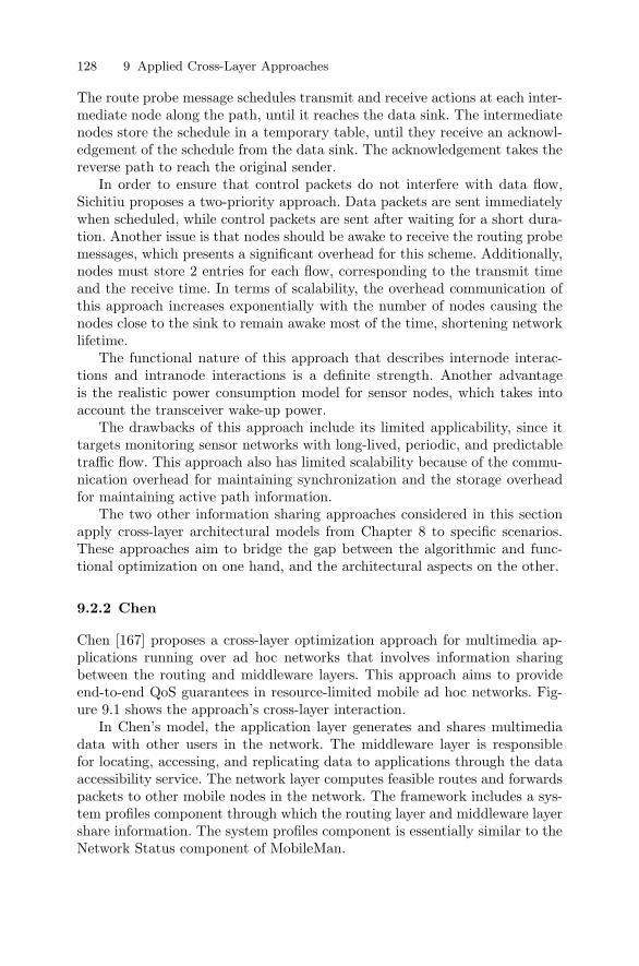
128 9 Applied Cross-Layer Approaches
The route probe message schedules transmit and receive actions at each inter-mediate node along the path, until it reaches the data sink. The intermediatenodes store the schedule in a temporary table, until they receive an acknowl-edgement of the schedule from the data sink. The acknowledgement takes thereverse path to reach the original sender.
In order to ensure that control packets do not interfere with data flow,Sichitiu proposes a two-priority approach. Data packets are sent immediatelywhen scheduled, while control packets are sent after waiting for a short dura-tion. Another issue is that nodes should be awake to receive the routing probemessages, which presents a significant overhead for this scheme. Additionally,nodes must store 2 entries for each flow, corresponding to the transmit timeand the receive time. In terms of scalability, the overhead communication ofthis approach increases exponentially with the number of nodes causing thenodes close to the sink to remain awake most of the time, shortening networklifetime.
The functional nature of this approach that describes internode interac-tions and intranode interactions is a definite strength. Another advantageis the realistic power consumption model for sensor nodes, which takes intoaccount the transceiver wake-up power.
The drawbacks of this approach include its limited applicability, since ittargets monitoring sensor networks with long-lived, periodic, and predictabletraffic flow. This approach also has limited scalability because of the commu-nication overhead for maintaining synchronization and the storage overheadfor maintaining active path information.
The two other information sharing approaches considered in this sectionapply cross-layer architectural models from Chapter 8 to specific scenarios.These approaches aim to bridge the gap between the algorithmic and func-tional optimization on one hand, and the architectural aspects on the other.
9.2.2 Chen
Chen [167] proposes a cross-layer optimization approach for multimedia ap-plications running over ad hoc networks that involves information sharingbetween the routing and middleware layers. This approach aims to provideend-to-end QoS guarantees in resource-limited mobile ad hoc networks. Fig-ure 9.1 shows the approach’s cross-layer interaction.
In Chen’s model, the application layer generates and shares multimediadata with other users in the network. The middleware layer is responsiblefor locating, accessing, and replicating data to applications through the dataaccessibility service. The network layer computes feasible routes and forwardspackets to other mobile nodes in the network. The framework includes a sys-tem profiles component through which the routing layer and middleware layershare information. The system profiles component is essentially similar to theNetwork Status component of MobileMan.
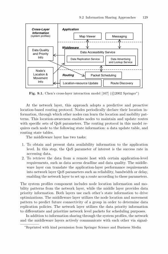
9.2 Information Sharing Approaches 129
Cross-Layer Information
(system profiles)
Data Quality and Priority
Info
Node’s Location & Movement
Info
Application
Middleware
Routing
Map Viewer Messaging
Data Accessibility Service
Data Replication Service Data Advertising and Lookup Service
Packet Scheduling
Location-resource Update Route Discovery
Fig. 9.1. Chen’s cross-layer interaction model [167] ( c©2002 Springer∗)
At the network layer, this approach adopts a predictive and proactivelocation-based routing protocol. Nodes periodically declare their location in-formation, through which other nodes can learn the location and mobility pat-terns. This location-awareness enables nodes to maintain and update routeswith specific sets of QoS parameters. The routing protocol in this model re-quires each node to the following state information: a data update table, androuting state tables.
The middleware layer has two tasks:
1. To obtain and present data availability information to the applicationlevel. In this step, the QoS parameter of interest is the success rate inaccessing data.
2. To retrieve the data from a remote host with certain application-levelrequirements, such as data access deadline and data quality. The middle-ware layer can translate the application-layer performance requirementsinto network layer QoS parameters such as reliability, bandwidth or delay,enabling the network layer to set up a route according to these parameters.
The system profiles component includes node location information and mo-bility patterns from the network layer, while the middle layer provides datapriority information. Both layers use each other’s state information to driveoptimizations. The middleware layer utilizes the node location and movementpattern to predict future connectivity of a group in order to determine datareplication policies. The network layer utilizes the data priority informationto differentiate and prioritize network level packets for scheduling purposes.
In addition to information sharing through the system profiles, the networkand the middleware layers actively communicate with each other via signal-
∗Reprinted with kind permission from Springer Science and Business Media
130 9 Applied Cross-Layer Approaches
ing regarding the condition of data transmission and adaptation. To adaptto minor network changes, the network layer can modify the current route,recompute another route, or notify the middleware layer of QoS violations incase no other route is available. In the latter case, the routing layer provideshints of currently available routes and their characteristics such as bandwidth,delay, and stability to the middleware layer. With these hints, the middlewarelayer can determine a proper higher-level adaptation strategy such as dataformat compression.
The cross-layer interaction and adaptivity of this approach perform wellfor small networks only. To achieve scalability, Chen et al. suggest floodingstate updates locally in a hierarchical topology, as suggested in [159].
In sum, Chen’s applied cross-layer approach confirms that informationsharing between the middleware and routing layers enable applications toachieve higher success rates in accessing data even in a highly dynamic adhoc networks.
9.2.3 Sensor Protocol
Polastre et al. propose an implementation of the Sensor Protocol (SP) [168]within the SP architecture (see Chapter 8). The proposed SP protocol imple-mentation attempts to provide a unifying abstraction that balances generalityand efficiency in sensor network design. In particular, it introduces interfacesfor efficient cross-layer information sharing between the MAC and routing lay-ers. The interfaces are designed to provide interoperability with a wide rangeof MAC and routing protocols, promoting innovation through code reuse.
The SP protocol implementation provides for three functionalities: datatransmission, data reception, and neighbor management. Whereas the first twofunctionalities are self-explanatory, neighbor management enables the routingand MAC layers to cooperate in managing internode interaction.
The interlayer interaction between the MAC and routing layers relies ontwo data structures: neighbor table, and message pool. The neighbor table is across-layer entity that enables the MAC and routing layers to store and shareneighborhood information, such as link states, route costs, and neighbor sleepand active schedules. The neighbor table thus serves as a common repositoryfor cross-layer state information, saving both storage space and access time tostate information. The second data structure in SP, the message pool, enablesnetwork protocols to request message transmissions on the basis of higherlayer quality requirements. Rather than storing actual messages, the messagepool contains references to messages, which can be accessed either in-order orout-of-order, depending on quality-of-service requirements. The network andMAC layers use the message pool structure to pass message information toeach other. For example, the network layer can set an urgent or a reliabilitybit for a particular message to force the MAC layer to aggressively attemptto meet the delay or reliability requirements for that message. The link layercan also send feedback to the network layer through the message pool. For
9.2 Information Sharing Approaches 131
instance, the link layer can communicate congestion or phase conflicts to thenetwork layer so that the latter can adjust its behavior accordingly.
A significant aspect of the SP protocol implementation is its focus onprogrammatic issues, such as code size, code reuse, and interlayer interfaces.The proposed SP protocol provides new interfaces for information sharingbetween generic MAC and network layers within the TinyOS [191] operatingsystem.
The main goals of this approach is to provide architectural modularityand interoperability while maintaining efficient network behavior for a wideset of network and data link protocols. To evaluate SP’s success in achiev-ing those goals, the authors perform experiments that couple SP with twoMAC protocols of distinct types: BMAC [56] (a channel sampling protocol),and IEEE 802.15.4 [189] (a slotted protocol). The experiments reveal thatthe SP abstraction layer provides modularity without any significant impacton data delivery for both MAC protocol types. The SP protocol also im-proves the adaptivity of the BMAC protocol, enabling nodes to adjust morequickly to surges in throughput requirements. Furthermore, deployment ex-periments illustrate that the introduction of the SP abstraction layer reducesthe average duty cycle of nodes for BMAC by more than 50%, through moreadaptive duty cycles1. The authors also consider three different routing pro-tocols (Mintroute [197], Trickle [169], and Synopsis Diffusion [170]) in theirperformance evaluation to verify that SP supports various network protocoltypes above it, in addition to its support for several MAC protocol types belowit.
The benefits of the SP protocol include its long-term vision for promot-ing innovation through a seamless cross-layer architecture. Another addedvalue of this approach is the consideration of implementation details, includ-ing data structures for cross-layer information sharing, programmatic issues,and storage complexity. A drawback of the proposed SP protocol is that itleaves several issues open, such as the sharing of timestamping, naming, andsecurity information across layers. To incorporate the additional cross-layerinformation, SP may require creating new data structures or extending theproposed data structures, which may cause the current SP memory footprintto overgrow existing storage resources at each node.
9.2.4 Jurdak
Jurdak [100] provides another example of a functional/architectural approachin the form of a general cross-layer framework for ad hoc and sensor networksthat provides both modularity and flexibility. The framework defines a gen-eral structure for implementing optimizations, and different applications cancustomize the frame work according to their performance requirements.1 Chapter 10 elaborates more on adaptive duty cycles with BMAC, as proposed
independently by Jurdak et al. [193].
132 9 Applied Cross-Layer Approaches
The modular design of Jurdak’s framework enables the use of any opti-mization algorithm to modify node configurations. The flexible node statedefinition enables customization for different applications. By choosing theconfigurations on which the algorithm operates, the framework can supportdifferent applications, quality goals, and communication technologies. The re-mainder of this section briefly demonstrates how customizing Jurdak’s generalframework to particular situations yields significant performance benefits. Inparticular, the framework is customized to three scenarios: monitoring andevent-driven RF sensor network test-bed; UWB ad hoc network; and acousticunderwater sensor network. Chapters 10, 11 and 12 discuss these 3 case inmuch more detail.
RF Sensor Network
The first scenario for this framework is a sensor network test-bed that uses RFwaves [100]. The network targets long-term monitoring deployments in whichthe sensor nodes periodically sample their sensors and send the data towards asingle base station. Because of the long-term operation requirement, the goalin this network is to promote energy efficiency through adaptive listeningmodes and to provide a longer network lifetime through load balancing.
To achieve these performance goals, this scenario relies on allowing sensornodes to power down their radio when they are inactive. In particular, nodesuse BMAC [56] to periodically check the channel for activity. The single datasink in the network yields a tree topology, placing more forwarding load atthe nodes close to the base station. As such, Jurdak’s approach introducesAdaptive Low Power Listening (ALPL), an algorithm which runs locally ateach node to enable the node to adapt their check interval according to theircurrent state. Unlike most other optimization algorithms, ALPL also spec-ifies the functional and implementation details including signalling, packetformats, and interfacing with existing mechanisms within the TinyOS [191]environment.
Referring back to Fig. 8.6, Jurdak’s framework consolidates three aspectsinto the node state for this scenario: (1) number of descendants in the routingtree; (2) radio duty cycle; and (3) node roles. The number of descendantsaspect quantifies the forwarding load of each node. The duty cycle aspectdetermines how busy a node’s radio has been during the recent time win-dow. Finally, the role aspect corresponds to the sensing and processing powerconsumption that may contribute to load imbalance in the network.
After collecting neighborhood state information, ALPL locally runs oneach node with the node’s overall state information as an input. Subsequently,ALPL locally adjusts the MAC layer listening mode and the routing cost ofneighbors. Performance evaluation on a deployed sensor network test-bed hasshown that Jurdak’s framework yields significant global energy savings andit effectively balances the load in this scenario. Chapter 10 elaborates furtheron this case study.
9.2 Information Sharing Approaches 133
UWB Ad Hoc Network
Jurdak’s framework is also customized for an UWB ad hoc network, resem-bling the network in [172]. This scenario targets QoS provision in UWB adhoc networks. The performance goals of this scenario are four-fold: (1) max-imize throughput; (2) promote fairness; (3) minimize link setup latency; and(4) minimize control overhead.
The spread-spectrum properties of UWB discussed in Section 9.1.9 implythat neighboring links can coexist, but they cause mutual interference. Tofully exploit these dependencies, this case study customizes Jurdak’s frame-work to provide a joint routing/MAC approach based on a broad node statespecification. The local state at each node combines interference, received ra-dio power, communication resource allocation for different traffic classes, andnode reliability. Nodes use this state information to adapt the transmissionrate and power of their active links in order to maintain quality guarantees.Nodes also adapt the neighbor costs and the period of their periodic hellomessages according to changes in local and neighborhood state.
Within the customized optimization framework, this scenario uses U-MAC,an adaptive MAC protocol for UWB networks in which nodes periodically de-clare their current state, so that neighbors can proactively assign power andrate values for new links locally in order to optimize global network perfor-mance. Simulations comparing U-MAC to the reactive link setup approachconfirm that U-MAC lowers link setup latency and control overhead, doublesthe throughput and adapts better to high network loads. For a more detaileddescription on this case study, please refer to Chapter 11.
Acoustic Underwater Sensor Network
The final scenario customizes Jurdak’s framework for an acoustic underwatersensor network. This scenario considers a network architecture in which sensornodes are deployed underwater to sample the environment. A single surfacenode acts as the gateway between the underwater nodes and the networkoperators. The underwater nodes communicate acoustically with each otherand with the gateway node, which is equipped with long range radio that cansend the data to a central repository on land. Thus, the logical topology ofthis network is also a tree topology centered at the gateway node.
The specific application of interest is the deployment of an underwateracoustic sensor network for environmental monitoring. The main challengeof deploying such a network is the limited battery resources of individualsensor nodes, which requires frequent retrieval and recharging of the node.Thus, the performance goal in this scenario is the maximization of networklifetime and the minimization of power consumption. This case study appliesJurdak’s optimization framework to an underwater acoustic sensor networkfor monitoring of a watershed in order to achieve the performance goal throughdistributed local decisions.
134 9 Applied Cross-Layer Approaches
The focus of the case study is the development of the optimization algo-rithm that maximizes battery life and minimizes energy consumption for anunderwater sensor network. The state parameters that affect energy consump-tion are: (1) internode distance; (2) transmission frequency; (3) frequency ofdata updates; and (4) number of descendants in the routing tree. Transmis-sion frequency and internode distances are both physical layer aspects. Thefrequency of data updates is an application layer aspect, and the number ofdescendants in the routing tree is a network layer aspect. The tree topologyof this network causes nodes close to the gateway to deplete their energy re-sources quickly. To address this issue, the algorithm enables the loaded nodesto select low transmission frequencies for their communication in order toreduce their power consumption. The rationale is that signal attenuation un-derwater depends on both distance and frequency. By assigning lower trans-mission frequencies to loaded nodes and higher transmission frequencies tounloaded nodes, the algorithm promotes load balancing and a prolonged net-work lifetime. The local and neighborhood state information can be employedlocally at each node to dynamically select the appropriate transmission fre-quency. Chapter 12 presents the details of this scenario.
9.3 Global Performance Goals
This section discusses the common performance goals of cross-layer approachesfor ad hoc and sensor networks. In other words, the focus of this sectionis to address the question: What performance goal is this particular cross-layer approach trying to achieve? Most approaches set performance goals ona network-wide basis to provide system-wide QoS guarantees. Some of theapproaches address tradeoffs between several performance goals, while othersfocus on a single performance goal. Each subsection in this section focuseson one performance goal, with a discussion of possible interactions with theother quality metrics.
9.3.1 Maximize Network Lifetime
One of the most common performance goals for ad hoc and sensor networksis to maximize network lifetime. Because resource-limited nodes must handleall aspects of network management in a distributed manner, all internode andinterlayer interactions in the network have a high impact on network lifetime.
For example, Girici’s approach [158] attempts to prolong network lifetimefor ad hoc networks by including the residual battery energy at each nodeinto the routing metric. This approach notes a significant increase in thenetwork lifetime (measured as the time of first node death) as a result of theinclusion of the residual energy metric. The inclusion of energy considerationsinto routing also yields a minor improvement of cumulative throughput at thetime the first node dies.
9.3 Global Performance Goals 135
Interestingly, the remainder of cross-layer approaches that aim to pro-long network lifetime all target sensor networks. For instance, Sichitiu’s ap-proach [171] considers a realistic power consumption model for sensor networksthat incorporates radio power consumption for idle listening, transmission andreception, sleep modes, and switching between modes. Within this approach,the routing and MAC layers can use the power consumption information foroptimizing their decisions in favor of network longevity. Sichitiu notes a sig-nificant degradation in network lifetime as a result of increased node density.
Madan et al. [163] also address the network lifetime performance goalsthrough cross-layer optimizations. Their approach considers the joint enforce-ment of mechanisms from the routing, MAC and physical layer such as multi-hop routing, load balancing, and interference mitigation to prolong networklifetime.
Finally, Jurdak [100] proposes an algorithm for prolonging the lifetime ofan underwater acoustic sensor network. Their algorithm analyzes underwateracoustic communication processes to develop a direct relationship betweenpower consumption for data transmission and reception on one hand, andnetwork battery lifetime on the other. The algorithm attempts to favor highlyloaded nodes near a base station through smart frequency channel assign-ments.
9.3.2 Energy Efficiency
The overwhelming majority of cross-layer approaches set energy efficiency asone of their performance targets [100,158–162,164]. Although energy efficiencyand lifetime maximization are closely correlated, the correlation is not alwayspositive. Consider a tree topology sensor network, as shown in Fig. 9.2. Mostof the routes that minimize energy consumption in the network may traversethe black node near the base station (Fig. 9.2(a)). Because this node hasto forward a large number of packets, it depletes its energy resources muchsooner than other nodes. In contrast, the routing graph in Fig. 9.2(b) opti-mizes network lifetime by balancing the network load among the three nodesnear the base station. This example demonstrates that the minimum energyrouting strategy does not necessarily correspond to the longest network life-time strategy.
The approach of Girici and Ephremides [158] addresses both issues of net-work lifetime and energy efficiency. They define network lifetime by the timeof the first node death. Their measure for energy efficiency is the energy ex-penditure per packet. Their findings reveal that including residual energy intothe routing metric prolongs network lifetime but it also increases overall powerexpenditure. In some cases, inclusion of the residual energy into routing deci-sions replaces minimum energy paths with maximum lifetime paths, tradingoff overall power consumption for network longevity.
Cruz and Santhanam [159] also target energy efficiency through anotherperspective on the tradeoff between energy efficiency and throughput in their

136 9 Applied Cross-Layer Approaches
(a) (b)
Fig. 9.2. (a) Optimal energy-efficient routing graph. (b) Optimal lifetime routinggraph.
cross-layer approach for wireless base stations. Using multiple paths for rout-ing data from source to destination shifts forwarding load away from hotspot nodes and increases throughput. However, multipath routing also causeshigher power consumption since it involves more intermediate nodes that mustforward data.
Other approaches focus on energy efficiency independently of lifetimeconsiderations. For example, Elbatt and Ephermides [160] focus on energy-efficient performance through a distributed power control algorithm thatyields the vector of minimum transmission powers for a given link schedule.Kozat et al. [161] approach the same energy efficiency problem, but they tryto generalize Elbatt and Ephermides’s 1-hop model to a multihop model. Con-sidering both a top-down and bottom-up approach for determining the linkschedule, Kozat et al. determine that the top-down approach of first solvingfor a feasible link schedule then determining transmission power assignmentsyield the highest performance. They also highlight the tradeoff between energyefficiency and other QoS metrics, such as delay and throughput.
Lu and Krishnamachari’s [162] approach attempts to formalize these trade-offs between energy efficiency, delay, and throughput through a tunable frame-work. In particular, the approach notes that relaxing the delay bounds in thenetwork could significantly improve energy efficiency. Determining the opti-mal weights of the three performance metrics can also lead to power savingswith no adverse effect on throughput.
Cui et al. [164] also address the energy delay tradeoff. Unlike previousapproaches, their approach incorporates both communication and hardwarepower consumption. This approach uses sleep modes and smart scheduling ofwake-up times for achieving energy efficiency.
9.3 Global Performance Goals 137
Jurdak’s [100] approach for RF sensor networks also uses sleep modes inthe form of low power listening modes to achieve energy efficiency. Unlikeschedule-based approaches, Jurdak’s approach requires no synchronization asthe underlying BMAC protocol matches nodes’ check interval and preamblelength to ensure delivery in asynchronous scenarios. In addition to this ap-proach’s explicit energy efficiency goal, it also implicitly prolongs networklifetime through load balancing.
Jurdak’s [100] applied framework to underwater sensor networks alsojointly addresses network lifetime and energy efficiency. Because the focusof this approach is to maximize the network lifetime, the lifetime maximiza-tion approach improves energy efficiency over the random case but it does notguarantee the highest energy efficiency.
9.3.3 Maximize Throughput
The main purpose of any network is data delivery. Ad hoc and sensor networksare no exception, which is why maximizing the data throughput is a commonperformance goal of five of the cross-layer approaches for ad hoc and sensornetworks in this chapter [100, 160, 162, 166, 172]. Interestingly, all but one ofthe approaches that optimize throughput rely on time synchronization and aslotted time structure. Furthermore, three of the five approaches [100,160,172]adopt a spread spectrum technology such as CDMA or UWB, highlighting thehigh bandwidth potential of these technologies.
For instance, Elbatt and Ephermides [160] emphasize the single hopthroughput in their approach. In particular, their approach optimizes thethroughput of individual outgoing time slots for a particular node. A jointCDMA/TDMA scheme provides a higher throughput than a pure TDMAscheme because it enables multiple concurrent transmissions on the same timeslot. The tradeoff of using CDMA is the added computational and hardwarecomplexity for transceivers.
Within their tunable framework for TDMA sensor networks, Lu and Kr-ishnamachari [162] define throughput as the number of packets that can betransmitted within a time frame. Because their scheme relies on TDMA, it canonly schedule concurrent transmissions that are spatially separated by somedistance. As such, the achievable throughput of this scheme is lower than theCDMA/TDMA scheme of ElBatt and Ephermides.
An alternate approach is the maximization of the bandwidth utilizationin the network while maintaining fairness among active sessions, as proposedin [166]. Unlike the other surveyed approaches that maximize throughput,Wang and Kar’s approach does not adopt a time-slotted structure. However,their approach does have a locally synchronous flavor represented by the pe-riodic update of link attempt probabilities. Another distinction of Wang andKar’s approach is its maximization of end-to-end throughput rather than thelocal node throughput.
138 9 Applied Cross-Layer Approaches
Both cross-layer approaches for UWB also target throughput optimization.Merz’s approach relies on interference mitigation for supporting a large num-ber of concurrent UWB links. The use of code rate adaptation also ensuresthat the nodes use the highest possible transmission rate supported by thecurrent interference levels. Jurdak’s approach for UWB ad hoc networks alsotries to maximize throughput through adaptation to interference levels in thenetwork, but it does so through power control rather than rate adaptation.This approach considers reserved bandwidth traffic that requires rate guar-antees in addition to best-effort traffic. The rate guarantees in the reservedbandwidth case do not allow rate adaptation, so power control is used to offerthroughput guarantees.
9.3.4 Minimize Delay
Delay is an important performance metric for time-sensitive applications, suchas multimedia delivery or emergency response. Cross-layer approaches typi-cally address delay as a tunable performance goal that involves tradeoffs withenergy and data delivery. Thus, delay has not been the primary performancegoal of cross-layer approaches.
For instance, Girici and Ephremides [158] represent link delay through arouting metric that quantifies the queue size at the sender. This delay routingmetric is part of a larger weighted routing cost function that enables differ-ent applications to set the metric weights on the basis of their performancerequirements. Lu and Krishnamachari [162] present a similar tunable frame-work that includes adjustable delay, energy, and throughput components. Toillustrate the delay energy tradeoff, this approach conducts simulations thatrelax the delay bounds to increase energy efficiency.
Finally, Jurdak’s approach for an UWB ad hoc network [100] explicitlyaddresses a single delay component: link setup delay. The approach outlinesmechanisms for reducing link setup latency through a reduction of hand-shaking requirements prior to setting up a new link. This approach implicitlyattempts to reduce queueing delay by enabling more concurrent links, therebyreducing the probability of deferred transmissions.
9.3.5 Promote Fairness
Optimizing certain performance metrics in the network may lead to unbal-anced resource allocation. For example, a greedy algorithm that enables anode to grab the largest available bandwidth may lead to bandwidth star-vation of other nodes. Another example is minimum energy paths, whicheventually leads to a shorter network lifetime because of overworked nodeson these paths.
Wang and Kar [166] subject their utility maximization approach to a pro-portional fair rate constraint. They attempt to balance bandwidth allocationsamong the active end-to-end sessions while maximizing bandwidth utilization.
9.3 Global Performance Goals 139
Another property that contributes to fairness in Wang and Kar’s approach isthat it evenly spreads bottleneck links in the network, which prevents band-width starvation of particular sessions due to overloaded links.
Jurdak’s approach [100] also addresses the fairness issue in the contextof an UWB ad hoc network. Because UWB is a spread spectrum technol-ogy, it has a soft capacity: concurrent transmissions can take place, but thetransmission rate of one link is highly sensitive to other neighboring links. Atnetwork startup, no links are active so the first node that has data to trans-mit establishes a link with a high transmission rate, corresponding to a hightransmit power (in order to maintain SNR at the receiver). Subsequent linksin the neighborhood can only use low transmission power, so their bandwidthis severely restricted. Additionally, UWB suffers from near/far effects evidentin other spread-spectrum technologies [17]. Nodes closer to a receiver typicallygrab a larger portion of bandwidth than nodes further away.
To mitigate these effects, Jurdak’s approach sets tunable margins on theportion of bandwidth and emitted power that each node can reserve. Themargins yield fairer access to the medium among near and far nodes. It alsoensures fairer transmission rates for link requests that arrive at different pointsin time.
9.3.6 Data Accessibility
From the perspective of multimedia applications running over mobile ad hocnetworks, data accessability is crucial for ensuring timely delivery and play-back of multimedia streams. Providing application with access to multimediadata often requires data replication across several nodes, so that if one nodemoves away or leaves the network, data forwarding and delivery can proceedunaffected. As discussed in Section 5.2, the middleware layer is responsiblefor data replication. However, the degree and locality of data replication in adhoc networks is highly dependent on the nodes’ mobility and locations [167],which are both routing layer aspects. Sharing information between the routingand middleware layers can lead to more efficient data replication, providing ahigher degree of data accessability and availability to applications.
9.3.7 Efficiency and Generality
Cross-layer proposals typically trade off generality and efficiency. For instance,design coupling approaches aim for optimizing behavior with little regard forinteroperability, architectural issues, or code reuse. The SP protocol [168]attempts to provide both efficiency and generality through an implementedinformation sharing approach. More specifically, it proposes and implementsan abstraction layer protocol for sensor networks, with a role similar to thatIP within the Internet. The SP design tries to share cross-layer informationbetween the MAC and network layers in a timely and reliable fashion, whilekeeping in mind the resource scarcity of sensor nodes. To balance generality
140 9 Applied Cross-Layer Approaches
and efficiency, SP provides cross-layer interfaces, such as for data transmissionand feedback, and cross-layer data structures, such as neighbor table andmessage pool, that are commonly employed by virtually all sensor networkand MAC protocols, emphasizing the generality aspect. Each protocol cancustomize its use of the common interfaces and message structures to achieveefficient behavior.
9.4 Target Networks
Cross-layer approaches are often designed with particular network scenariosin mind. From example, many approaches adopt a slotted time model andassume that nodes can synchronize their clocks. The optimization algorithmitself builds on the target network model and the underlying assumptions. Assuch, understanding the benefits of each applied cross-layer approach partiallyrelies on considering its network target scenario. This section classifies anddiscusses applied approaches based on their target network choice. The cross-layer approaches target 2 broad classes of networks: ad hoc networks, andsensor networks.
9.4.1 Ad Hoc Networks
Cross-layer approaches that target ad hoc networks [100, 158, 160, 161, 166,172] fall into 4 categories: TDMA ad hoc networks, UWB ad hoc networks,multimedia ad hoc networks, and general ad hoc networks.
TDMA Ad Hoc Networks
The main characteristic of a TDMA-based ad hoc network model is the notionof fixed time slots for channel separation. TDMA-based approaches in theliterature also share the following features:
• Synchronization: all models assume that node clocks are synchronized.Synchronization is an essential component of any TDMA-based approach
• Stationary nodes: all of these models assume that nodes are stationaryfor their optimizations. Although this assumption grounds the optimiza-tion problem, it also limits the applicability of the proposed approaches toa wide range of mobile ad hoc network applications
• Sender-initiated communication: another shared assumption is source-oriented communication. This assumption models the intermittent commu-nication trend in many ad hoc networks, as opposed to the regular dataflow in monitoring or real-time networks
• Transceiver power: all models place a limit on the transmission poweras a constraint for the optimization problem, focusing on determining theoptimal transmission power for given link schedules
9.4 Target Networks 141
• Omnidirectional antenna: all models assume omnidirectional antennas,which is the simpler and cheaper choice. Directional antennas could enablefurther optimizations, but they add hardware complexity and cost
In addition to the common features of TDMA-based cross-layer ap-proaches, individual models have made further assumptions for developingtheir optimization algorithm. For example, a functional requirement of mostTDMA-based approaches is a dedicated control channel in the form of a re-served time slot [158]. The control channel enables reservation and schedulingof other time slots for data transmissions. This is a reasonable assumptionsince the only cost involved is the allocation of time slots for control messag-ing.
Another assumption that facilitates routing is the availability of geographicinformation at the nodes [160]. Nodes can narrow route searches to morespecific geographic regions, thereby preserving resources (see Section 4.5).Providing nodes with geographic information requires additional positioningmechanisms at the nodes, such as GPS.
UWB Ad Hoc Networks
Two of the cross-layer approaches in the literature target UWB ad hoc net-works [100, 172]. Both of these approaches target time-hopping UWB net-works, and they perform their evaluations in a stationary environment. Addi-tionally, both models consider the spread-spectrum nature of UWB transmis-sion for determining the signal quality at a receiver, which is dependent onthe active transmissions in the vicinity of the receiver. As such, both modelstackle the problem of assigning the optimal transmission parameters of a newlink while preserving the quality requirements of the active links.
What differentiates the two models are the assumptions of the tunabletransmission parameter. Merz et al. consider that nodes always transmit withthe maximum transmission power, and they regulate the transmission rateto achieve an acceptable SNR at the receiver. In contrast, Jurdak’s approachconsiders two traffic types: reserved bandwidth (RB), and dynamic band-width (DB). The RB traffic class requires rate guarantees, so the approachadjusts transmission power while providing a constant transmission rate. TheDB class supports best-effort traffic, enabling an elastic rate adjustment with-out changing transmission power. The DB traffic case of Jurdak’s approachresembles Merz’s model, while the RB traffic class provides support for higherpriority traffic.
Another difference between the two approaches is that Jurdak assumesthe presence of a separate TH-code for control signalling that is known toall nodes. Merz considers that each receiver owns its own TH-code, and thatsenders target the receiver by using the receiver’s TH-code. While Merz’sapproach is more scalable with network size, it also requires nodes to learnand store the state of all potential neighbors. In dynamic or mobile networks,the overhead of this approach may overweigh the benefits.
142 9 Applied Cross-Layer Approaches
Multimedia Ad Hoc Networks
One application for connection-oriented ad hoc networks is the transport ofmultimedia streams. The stringent rate and deadline requirements of mul-timedia applications complicate the task of running these applications overmobile ad hoc networks. Because ad hoc network nodes may enter, leave, ormove around within the network, Chen et al. [167] propose cross-layer inter-action between the routing and middleware layers to increase data availabil-ity for multimedia applications. The basic premise of their approach is thatmultimedia applications have higher priority over regular data, and differentmultimedia streams may have various degrees of priority among them. Pro-viding the routing layer with visibility into the priority of multimedia streamsenables delivery of urgent packets first. Similarly, the middleware layer canexploit routing layer information, such as node locations and mobility, in or-der to adapt data compression rates or to replicate data to ensure availabilityto multimedia applications.
General Ad Hoc Networks
Wang and Kar [166] consider the problem of maximization the bandwidthutilization for end-to-end sessions in multi-hop wireless ad hoc networks. Thisapproach maintains generality as it makes no assumptions on time synchro-nization between the nodes or regarding the target application or underlyingphysical layer technology. The only assumption in Wang and Kar’s approachabout the target scenario is the symmetric hearing matrix, which assumesbidirectional links. In practice, assuming that all links are bidirectional limitsthe scope of the approach to ad hoc networks with highly reliable links andfew physical obstacles.
9.4.2 Sensor Networks
Recently, researchers have proposed cross-layer approaches specifically for sen-sor networks [100, 162–164, 168, 171]. What distinguishes sensor network ap-proaches from general ad hoc network approaches are the assumptions of acommon network-wide goal, data flow towards one or few sinks, and mostlystationary nodes. Sensor network approaches fall into two broad categories:TDMA-based approaches and non-TDMA approaches.
TDMA Sensor Networks
Cross layer approaches for sensor networks that rely on a TDMA structureare suitable for networks with regular and frequent traffic. As in the caseof TDMA-based ad hoc network approaches, TDMA-based sensor networkapproaches adopt a slotted time structure. Most of the other assumptions ofTDMA-based ad hoc networks also apply for TDMA sensor networks. We
9.5 Input Aspects 143
note here that maintaining node synchronization in sensor networks could beeven more costly in dense or dynamic networks, resulting in less efficient usageof the scarce node resources.
Non-TDMA Sensor Networks
Approaches for non-TDMA sensor networks [100, 168, 171] do not assumeany time-slotted structure for transmissions. In general, these approaches aremore suitable for long-term monitoring networks in which nodes sample theirsensors and send data infrequently or asynchronously, switching into low-power sleep modes when they are not active.
Despite its support for asynchronous data transmission, Sichitiu’s ap-proach assumes that nodes synchronize their clocks for establishing sleep andwake-up schedules for transceivers. The authors also show that a decreasein synchronization precision does not significantly degrade their approach’sperformance.
Both the SP protocol and Jurdak’s approach move away from the synchro-nization approach altogether. Both works adopt adaptive and asynchronouslistening modes, ensuring that nodes can turn off their transceivers for mostof the time while still hearing all relevant data and control packets. The keyconcept is to enable a sender to send packets with the appropriate preamblelength to match the receiver’s check interval. What distinguishes the two ap-proaches are the factors that determine the preamble length. Whereas the SPprotocol determines the preamble length purely on the channel state, Jurdak’sapproach combines aspects from across the network stack, such as a node’srole and its number of descendants, in order to determine listening modes andpreamble lengths.
9.5 Input Aspects
As in most algorithms, optimization decisions in cross-layer approaches rely oninput information about the state of nodes, links, or the network as a whole.What distinguishes cross-layer approaches from strictly layered approaches isthat the input state information comes from several layers across the com-munication stack. Consolidating state information across traditional layersenables deeper and more granular performance gains. Although cross-layerapproaches advocate a shift away from strict layers, providing smooth transi-tions from traditional layered approaches to cross-layer approaches begins bymapping the information used in cross-layer approaches to the original layersin traditional approaches. Each subsection examines the input state variablesof cross-layer approaches based on their layer classification in traditional lay-ered architectures.
144 9 Applied Cross-Layer Approaches
9.5.1 Application Layer
Cross-layer approaches that incorporate application layer variables into opti-mization decisions make inherent assumptions about the target application.From Tables 9.1 and 9.2, we note all the approaches that use input infor-mation from the application layer are information sharing approaches, andthree of these four approaches target monitoring sensor networks [100, 171].Monitoring sensor networks assume the presence of one or a few data sinks,and that sensors periodically sample and send data towards the data sink.The remaining approach that uses application layer information considers atechnology-specific network (UWB) which entails implicit assumptions on theapplication, including a short-range high bandwidth scenario.
Current approaches also differ with their choice of application input stateinformation. For example, Sichitiu’s sensor network approach [171] allowsgeneric applications to determine next hop information, without specifyingthe nature of the application variables. Jurdak’s approach for UWB ad hocnetworks [100] obtains the Mean Time Between Failures (MTBF) variablefrom the application layer. MTBF is a variable through which an applicationquantifies the communication and functional reliability of a node [175].
Other approaches use sensor-network specific variables. In particular, thework in [100] uses the node’s data reporting frequency, available locally, asan input to the battery lifetime optimization method. Adaptive Low PowerListening [100] includes information about each node’s role to determine thenode’s optimal check interval. For example, nodes that detect a fire in a forest-fire monitoring network adopt a reporting role and begin sampling their sen-sors more frequently. Such nodes can use role information for adjusting theirlistening modes.
9.5.2 Middleware Layer
One of the surveyed approaches [167] uses input information from the middle-ware layer for cross-layer optimizations. In their approach, Chen et al. providethe data priority information from the middleware layer to the routing layerto enable priority-based routing of data packets. The provision of middlewaredata priority information enables the network layer to establish routes thatprovide QoS guarantees.
9.5.3 Transport Layer
So far, there has been no documented use of transport layer information asinput for cross-layer optimizations for ad hoc or sensor networks. However,one can envision scenarios that use transport layer information, such as con-gestion windows or timeout values to prioritize packet delivery at the routingor data link layer. As cross-layer approaches start to shift from algorithmic toarchitectural nature, we expect that there will be more cross-layer approachesthat exploit transport layer information in the foreseeable future.
9.5 Input Aspects 145
9.5.4 Network Layer
Half of the surveyed cross-layer approaches for ad hoc and sensor networksinclude network layer information as input into their optimization decisions.Network layer information can benefit end-to-end and per-link throughput,delay, and energy consumption.
In the simplest case, nodes in a tree topology network (which is commonin sensor networks) can use information on their hop count from the treeroot (the base station) for communication decisions. For example, nodes canuse their basic hop count information along with specialized control messagesfor setting up non-conflicting link schedules in a sensor network [171].
A similar network layer metric that applies for tree topology networks isthe number of descendants in the tree [100,163,171]. Because data flow in thesenetworks flows towards the base station, a node’s number of descendants in therouting tree indicates its forwarding load. Leaf nodes have no forwarding load,while nodes that are close to the base station have a relatively large forwardingload. Using descendant information enables nodes to adapt network behaviordistributively to favor highly loaded nodes. For example, nodes can shift awaytheir traffic from highly loaded nodes [100]. In an underwater network, nodeswith higher load can use lower transmission frequencies, thereby reducing theirpower consumption [100].
Routing queue length is another network layer variable used in cross-layeroptimizations. Girici and Ephremides [158] demonstrate that including thequeue length into the routing metrics yields the best delay performance intheir joint routing and scheduling optimization scheme.
In mobile networks, location and mobility information are important rout-ing aspects that affect performance of several layers of the communicationstack [167]. For example, mobility and location may affect collisions and chan-nel access variables at the MAC, or data accessability at the application layer.Location and mobility are particularly important for multimedia applicationsthat require a high degree of data availability to meet rate and delay guaran-tees.
Simple network layer attributes, such as reliability or urgency, can alsoplay a role in determining the behavior of other layers. The network layer inSP [168] informs the link layer of message reliability or urgency merely bysetting the corresponding bit values in available cross-layer data structures.SP’s use of only two bits for communicating these network layer attributescan instruct the link layer on how to handle the messages without addingappreciable storage overhead.
Finally, nodes can exploit the end-to-end bandwidth requirements for op-timizing their behavior. For example, Jurdak’s approach for UWB ad hoc net-works tags traffic as either reserved bandwidth or dynamic bandwidth traffic.Nodes can use the traffic rate guarantees (or the lack thereof) at the physicallayer for adjusting the link transmission rate or the link transmission power.
146 9 Applied Cross-Layer Approaches
9.5.5 Data Link Layer
The importance of the state of a nodes’ wireless links has led researchers toinclude data link layer information into their cross-layer models. For exam-ple, the routing layer can exploit link layer information for choosing routesthat provide throughput guarantees. Girici and Ephremides [158] incorporatea link’s overall throughput during the network lifetime as a weighted routingmetric. Their scheme favors outgoing links that can support high through-put routes. Each node can execute this cross-layer algorithm locally, yieldinghigher network throughput. A similar approach is to use a dynamic measureof link quality for determining optimal routes, as suggested in [171].
The average long-term link data rate is another data link layer metric forcross-layer optimizations. The approach in [159] uses each link’s average datarate as an input to solve the joint scheduling and power control problem. Inother words, this approach exploits cross-layer interaction between the av-erage link data rate variable (a data link layer aspect) to determine, amongother things, the transmission power configuration at the physical layer. Kozatet al. [161] provide a similar cross-layer coupling through their considerationof short-term end-to-end rates for choosing transmission power in attemptto provide a more adaptive model for ad hoc networks. Wang and Kar’s ap-proach [166] provides the option of slow or faster adaption of the session ratesat the transport layer and the link rates at the data link layer to the existinglink attempt probabilities.
In networks with adaptive duty cycles, the active and sleep schedules ofnodes play a significant role in determining communication behavior. Twocross-layer approaches [100, 168] use the sleep and active schedule of neigh-bors in order to determine the preamble length for the BMAC protocol. Theavailability of neighbor schedule information locally enables a node to saveon energy consumption, either through the use of short preamble packets orthrough the reduction of packet retransmissions caused by mismatches be-tween the sender and receiver.
Finally, one cross-layer approach [100] has exploited the radio duty cycleinformation from the data link layer. This approach enables nodes to learnthe radio duty cycles of its one-hop neighbors and to set neighbor routingcosts in a manner that favors nodes with lower radio duty cycles. The newrouting costs shift traffic away from busier nodes, enabling the busy nodes toput their transceivers in sleep mode more often.
9.5.6 Physical Layer
The most widely used input variables for cross-layer approaches originate atthe physical layer. Cross-layer approaches can exploit physical layer informa-tion, such as transmission rate or transmission power, for guiding decisions athigher layers, such as link scheduling or routing choices.
9.5 Input Aspects 147
Physical layer variables for cross-layer approaches fall into several cate-gories: power consumption variables, transmission quality variables, and localnode energy variables. Power consumption variables include power consump-tion for transmission, processing, sensing, as well as for other node hardware.Transmission quality variables indicate the physical layer quality requirementsof a link, such as the desired SNR and the tolerated BER. Finally, the localenergy variables include the residual battery energy at the node, and anypotential energy harvesting gains.
Power consumption variables dominate the physical layer input variables.In particular, many approaches adjust the transmission power for cross-layeroptimizations. One approach is to assume that each link uses the lowesttransmission power possible to achieve error-free communications, as in [158].Other approaches subject links to a maximum link transmission power con-straint [100, 159, 165]. Interestingly, the approach in [172] remarks that op-timality calls for using the maximum transmission power for every link, soit adopts a fixed transmission power strategy that always uses the highesttransmission power.
Other examples of power consumption variables include processing, cir-cuit and sensing power consumption. Circuit power consumption becomes asignificant power sink for short-range networks in which transceiver poweris relatively low [165]. As such, Cui’s approach considers circuit processingpower in its minimization of network power consumption. A similar reasoningfor sensor networks [100] raises the need to consider the non-negligible sensingpower consumption for energy optimizations.
Most approaches attempt to minimize power consumption without violat-ing physical layer quality metrics, such as a minimum acceptable SNR or amaximum BER. ElBatt and Ephremides [160] develop their joint schedulingand power control algorithm to satisfy a set of SNR requirements. Anotherapproach to the same optimization problem uses maximum BER constraints,assuming BER is monotonically decreasing with increasing SNR [161]. In ad-dition to using SNR as a feasibility constraint for the solution of a cross-layeroptimization problem, both algorithms in [162] and [163] also rank potentiallinks according to their achievable SNR. As the algorithms progress, they at-tempt to generate a feasible transmission scenario from an infeasible scenarioby deferring links with low SNR.
UWB networks have their own SNR definition which accounts for the in-terference from all concurrent transmissions. Because feasibility of new UWBlinks requires a minimum SNR for the new link and maintaining the feasibilityof ongoing links, Jurdak’s approach proposes that nodes establish links witha SNR that is higher than the minimum SNR by some margin. The margin isdependent on the network density, and it mitigates both bandwidth starvationand link quality violations.
Another approach for UWB ad hoc networks [172] considers the difficultyof computing the receiver SNR for a new link at the sender. Instead, Merz’sapproach enables a sender to progressively discover the best transmission time
148 9 Applied Cross-Layer Approaches
and optimal code rate through repeated transmissions on the receiver’s TH-code.
Finally, Girici and Ephremides [158] consider the residual energy metricfrom the physical layer to guide routing decisions. Nodes with lower residualenergy levels are avoided in routing paths. The drawback of using the residualenergy metric, usually quantified by the battery voltage, is that small batterydischarge trends involve fluctuations as the voltage level drops, which maylead to routing flaps.
This section has discussed the input variables considered by cross-layerapproaches for ad hoc and sensor networks. Cross-layer approaches operateon the input variables to determine the optimal values for a set of variablesand configurations. The next section examines these output variables andconfigurations.
9.6 Configuration Optimizations
Most of the existing cross-layer approaches have focused on optimizing con-figurations that span the first three layers of the communication stack, whileresearch has been limited on adjusting configurations at higher layers for net-work optimization. The following factors explain this trend:
• The application layer typically sets the requirements for the rest of thelayers. Thus, the application layer variables serve as inputs rather thanoutputs for the cross-layer optimization approach
• While there has been a body of research on transport protocols for adhoc and sensor networks (see Section 5.1), the reliability, flow control, andcongestion control mechanisms are not as crucial for the operation of adhoc and sensor networks as lower layer functionality
• The network, data link, and physical layers constitute the core of networkoperation and interactions. The distributed management requirement ofad hoc and sensor networks has the deepest impact on these three layers,bringing them to the forefront of optimization efforts.
Each subsection in the remainder of this section discusses the optimization ofnetwork configurations at a single layer.
9.6.1 Middleware
Among the fifteen surveyed cross-layer approaches in this chapter, Chen’s ap-proach is the only one that optimizes the configuration at the middlewarelayer, violating the prevailing trend of lower layer optimizations. Through theuse of location and mobility information from the routing layer, the middle-ware layer predicts network connectivity. As such, the middleware layer adaptsdata replication policies to ensure data is available for the active applications.
9.6 Configuration Optimizations 149
The approach also modifies middleware configuration based on current routequality. If the transmission quality over a certain route drops, then the mid-dleware layer can adapt data compression rates to better fit the degradedroute quality.
9.6.2 Transport Layer
Wang and Kar’s approach [166] represents another example of cross-layer op-timizations that target higher layers, through its joint optimization of thetransport and data link layer configurations. In particular, their approach fo-cuses on the optimization of the end-to-end session rates according to the ob-served neighborhood link rates. Nodes periodically measure their current linkattempt probabilities and compute their link rates. These values are sharedwith the transport layer which can then proceed to compute the optimal end-to-end rates of active sessions on the basis of the current link conditions.
9.6.3 Network Layer
About half of the surveyed cross-layer approaches attempt to optimize thenetwork layer configuration. All of these approaches set the routing costs in amanner that promotes their global performance goals.
The most common approach is the use of compound routing cost functionsthat combine several weighted route metrics [100, 158]. Weighted cost func-tions are tunable to fit different application needs, by adjusting the weights ofthe cost function components. In one approach, the cost function integratesenergy-related metrics, such as radio duty cycle and sensing duty cycle, aswell as hop count and link quality. The cost function can also take a morecomprehensive definition that includes reliability, delay, and throughput fromacross the communication stack [100,158].
Another class of approaches algorithmically derives the routing cost as ajoint metric that embodies power and link scheduling considerations [159,165,171]. The resulting routing cost for each link is then used with a traditionalrouting algorithm, such as a shortest path algorithm, to determine optimalpaths.
Yet another perspective is to prioritize packet forwarding at the routinglayers according to higher layer priorities, as suggested by Chen et al. [167].Because applications may differ in their quality-of-service metrics, such as end-to-end rate or delivery deadlines, the routing layer may use this applicationlayer information to prioritize urgent packets over other packets in an attemptto meet the QoS requirements of all active multimedia streams.
Finally, nodes can adjust their route flow rates based on cross-layer infor-mation sharing, as suggested in SP [168]. Within the SP proposal, feedbacknotifications from the data link layer can inform the network layer of con-gestion or phase conflicts on particular links, enabling the network layer toadjust data rates or to shift the transmission phase for those links.
150 9 Applied Cross-Layer Approaches
9.6.4 Data Link Layer
All but one of the surveyed cross-layer approaches optimize the configurationof the data link layer, highlighting the instrumental role of the data linklayer for optimal behavior in ad hoc and sensor networks. Data link layeroptimizations range from link schedules to the adjustment of duty cycles andtimers.
Link schedules are an important output of cross-layer approaches thattarget TDMA-based networks. The main link schedule problem is to scheduleas many concurrent transmissions as possible while satisfying transmissionpower constraints [159–162]. In some cases, routing considerations [158, 163,171] or circuit power [165] also constrain the link schedule. Because TDMAapproaches structure time into slots and frames, optimizing link schedulesreduces to determining the optimal assignment of links into time slots withinthe problem constraints. One set of approaches attempts to progressively fillavailable time slots evenly, while another set tries to maximize the scheduledlinks in one time slot before trying to fill another slot.
Wang and Kar’s approach [166] optimizes link attempt probabilities ratherthan link schedules, since it relies on a probabilistic asynchronous approachrather than time synchronization. This approach begins with the current linkattempt probabilities as an input, and it iteratively computes the optimal end-to-end session rates and the corresponding new link rates. SP [168] is anotherapproach that relies on asynchronous link scheduling. Through its messagepool data structure, SP enables the link layer to forcefully schedule certainmessages or to send packets out-of-order for meeting network layer qualityrequirements, such as reliability or urgency.
A prominent trend among cross-layer approaches that target UWB ad hocnetworks is to dynamically optimize data link layer timer values according tonetwork conditions. For example, the data link layer in Merz’s approach [172]determines when and how to set back-off timers after probing the receiver’sTH-code. In another example, nodes in Jurdak’s approach [100] periodicallyrecompute the value of the timer for the hello messages depending on therate of change of neighbor states. In a completely asynchronous approach,ALPL [100] enables each node to determine its optimal low power listeningmode according to its number of descendants in the routing tree, indicatedby the forwarding load.
9.6.5 Physical Layer
Most cross-layer approaches also attempt to optimize the physical layer con-figuration. Adjusting transmission power, transmission rate, or modulationparameters are common techniques for physical layer optimization.
The majority of cross-layer approaches that target physical layer configu-ration enable nodes to tune their transmission power to satisfy constraintsincluding long-term or short-term transmission rates [159, 161] or routing
9.7 Implementation 151
flows [158, 171]. The basic premise is that each transmitter has a maximumallowable power emission, set by hardware limitations or regulatory bodies.The goal is the adjustment of transmission powers in the network, withinthe maximum transmission power constraint and the constraints from otherlayers, to achieve feasible power assignments for all transmissions.
Another direction is to consider the joint adjustment of transmission powerand transmission rates to satisfy the higher layer constraints. For example,Jurdak’s UWB approach [100] considers two traffic classes: a rate-guaranteedclass, and a best-effort class. For the rate-guaranteed class, power can beadjusted to maintain acceptable transmission rates. In contrast, transmissionrates are elastic for the best-effort class and they vary according to interferenceconditions to maintain a constant transmission power. Another example isthe joint computation of transmission powers and rates given a set of fixedrate requirements [163]. Nodes can select the transmission rate and power formultiple outgoing links to deliver the data to the destination through multi-path routes.
Alternative approaches manipulate the code rate at the transmitter to sat-isfy network constraints. Cui et al. [165] determine the upper and lower boundsof their Multiple Quadrature Amplitude Modulation (MQAM) rate, as well asthe transmission power. The minimum modulation rate is constrained by SNRconsiderations, while the maximum transmission power sets the upper boundfor modulation rate. In a similar approach that is designed for UWB technol-ogy, Merz [172] determines the maximum usable TH-code rate that mitigatesinterference at neighboring links. In another technology-dependent approachfor underwater acoustics, Jurdak [100] adjusts the transmission frequency ofacoustic transceivers to favor highly loaded nodes. This optimal transmissionfrequency choice depends on sensor update period, routing flows, as well aspropagation loss considerations.
9.7 Implementation
One of the more practical aspects of cross-layer optimization approaches isthe proposed implementation strategy. The implementation strategy specifiesthe internode and interlayer interactions, as well as computational details ofsupporting the proposed approach. Naturally, a deeper specification of imple-mentation strategy results in a more readily applicable approach. This sectionclassifies the existing cross-layer approaches into three categories based ontheir implementation strategy: unspecified, centralized, and distributed.
9.7.1 Unspecified
Some approaches focus on obtaining an optimal solution to a cross-layer prob-lem without specification of any implementation details [14,158,162,163,165].
152 9 Applied Cross-Layer Approaches
The main advantage of these approaches is that they typically focus on devel-oping computationally efficient algorithms that can scale for large networks.The tradeoff for the focus on algorithmic development is that implementationdetails remain unresolved.
Most of the approaches with an unspecified implementation rely solely ontheoretical analysis and design coupling without alluding to practical imple-mentation aspects which are significant in the emerging research field of adhoc and sensor networks. For example, these approaches derive polynomialor exponential order optimization algorithms that couple the functionalitiesof several layers. However, many nodes in ad hoc and sensor networks maylack the resources for running these algorithms, which leaves an open questionabout the applicability of these approaches in practical scenarios. Cross-layerapproaches with unspecified implementation strategies also neglect the designof internode protocol interactions and the intranode layer interactions.
Most of these approaches make simplifying assumptions for their optimiza-tion algorithms. For example, several approaches [158, 162, 163, 165] assumenode synchronization, but the absence of implementation details means thatit is up to the network programmer to figure out the hardware and softwarerequirements to achieve synchronization.
The performance evaluation of cross-layer approaches with an unspecifiedimplementation strategy rely on numerical examples [165], numerical simu-lations [14, 162, 163], or queueing models [158]. Although this type of perfor-mance evaluation provides theoretical validation, the performance evaluationof these approaches does not address practical issues such as interference ordynamic deployment environments.
9.7.2 Centralized
Centralized implementation strategies specify that the optimization algorithmruns at a central controller [160,161]. Because of the lack of a central controllerin ad hoc and sensor networks, developing cross-layer approaches for ad hocand sensor networks with a centralized implementation strategy is certainlyan interim step towards the development of fully distributed schemes.
Cross-layer approaches with a centralized implementation strategy assumethat the central controller has a global view of the network state. By run-ning the optimization algorithm, the central controller can notify each nodeof its optimal configuration. Of course, dynamic network conditions dictatethat the collection of network state and the dissemination of node configu-rations is repeated periodically, which is not in a scalable solution for largenetworks. ElBatt and Ephremides [160] attempt to partially mitigate this is-sue by distributing power control computations to the nodes while runningthe scheduling algorithm centrally.
9.8 Conclusion 153
9.7.3 Distributed
Distributed implementation strategies are more suitable for ad hoc and sensornetworks, as they spread the communication and computation among thenodes. Interestingly, five out of six applied information sharing approachesadopt a distributed implementation strategy, compared to only 33% of designcoupling approaches.
Cruz and Santhanam’s approach [159] provides limited implementationdetails for wireless base stations. This approach adopts a hierarchical clusteredtopology where link schedules of each cluster are determined independently,and then clusters collaborate to determine further dependencies. Althoughthis approach has a distributed computational and collaboration strategy, itfalls short of specifying the internode and interlayer interactions to support thedistributed strategy. Taking a step further, Wang and Kar’s approach [166]specifies the required interlayer interaction between the transport and thedata link layers in order to optimize session and link rates respectively. Thisapproach also supports distributed computation at each node, but it fallsshort of specifying the internode protocol interaction details in relation to thecross-layer optimizations.
Another class of approaches adopts a fully distributed strategy and spec-ifies protocol and interlayer interactions. For example, Sichitiu’s cross-layerapproach [171] describes all the distributed computation, control messaging,phases for forming paths, scheduling links, and handling failures to maximizethe lifetime of monitoring sensor networks. Chen et al. [167] adopt a fully dis-tributed data advertising and lookup service, which, in conjunction with theirmiddleware/routing cross-layer approach, supports data replication and en-sures data accessability for multimedia applications. Similar fully distributedcross-layer approaches include SP [168] and ALPL [100], which both enablenodes to determine optimal listening modes locally based on local and neigh-bor states. The evaluation of both approaches was conducted on test-beds ofsensor nodes, enabling a more realistic observation of these approaches in apractical scenario.
Other distributed cross-layer approaches targeting UWB ad hoc net-works [100, 172] provide a similar specification of the control messaging, lo-cal node computation, and link failure and deferment to maximize networkthroughput and promote fairness. These approaches require nodes to learnpartial state of the network in order to locally compute their optimal config-urations. All of these distributed approaches demonstrate their applicabilityand performance through network simulations that model interlayer interac-tions and the internode interactions.
9.8 Conclusion
This chapter has surveyed existing cross-layer approaches for ad hoc and sen-sor networks. After a brief overview of each approach, the approaches were
154 9 Applied Cross-Layer Approaches
classified and analyzed according to five different features: (1) performancegoals; (2) target network; (3) input aspects; (4) optimizations; and (5) imple-mentation. The most common performance goals are energy-related aspects,such as network lifetime or energy efficiency. Cross-layer approaches have tar-geted different network types, including TDMA ad hoc or sensor networks,UWB ad hoc networks, underwater acoustic sensor networks, and RF sen-sor networks. Most of the input aspects originate from the first three layers,while some approaches also include application or middleware layer aspectsas input to their optimization algorithm. The optimizations of almost all ap-proaches are restricted to the physical, data link, and network layers. Finally,we have discussed the implementation strategy of the surveyed approaches,noting that distributed strategies are the most appropriate for ad hoc andsensor networks.
The next part of the book focuses on three applied diverse case studiesof Jurdak’s cross-layer optimization approach for different target networks:RF sensor network, UWB ad hoc network, and underwater acoustic sensornetwork. For each case, we specify the performance goals, input aspects, op-timizations, and implementation strategy, before presenting the optimizationalgorithms, protocols, or heuristics.

Part III
Case Studies
10
Optimization of an RF Sensor Network
This case study applies Jurdak’s framework to a test-bed of sensor nodes thatcommunicate through RF signals. In particular, we explore the benefits ofthis approach in reducing the idle listening at individual nodes in order toreduce the energy consumption and to balance the forwarding load amongnetwork nodes. Our study introduces Adaptive Low Power Listening (ALPL),an adaptive cross-layer mechanism that builds on BMAC [56] in order to en-able individual nodes to seamlessly adapt their listening modes to their localstates. The chapter identifies three state aspects that impact energy consump-tion: (1) number of descendants in the routing tree; (2) radio duty cycle; and(3) role. We conduct experiments on a test-bed of 14 mica 2 sensor nodesto compare the state representations and to evaluate the framework’s energybenefits. The experiments show that the degree of load balancing increases forexpanded cross-layer state representations. The experiments also reveal thatall state representations in Jurdak’s framework reduce global energy consump-tion in the range of one-third for a time-driven monitoring network, and inthe range of one-fifth for an event-driven target tracking network.
10.1 Introduction
Most conventional networks have many users, with each user having theirindividual application objectives. As a result, optimization in conventionalnetworks has often focused on providing performance guarantees on a per-useror per-connection basis. In sensor networks, the nodes collaborate to achievea common network-wide goal. As such, sensor networks must provide globalnetwork performance guarantees instead of providing user-specific or node-specific performance guarantees, suggesting the need for global optimizationmechanisms.
Portions reprinted from (R. Jurdak. “Modeling and Optimization of Ad Hoc andSensor Networks,” Bren School of Information and Computer Science, Universityof California Irvine. Ph.D. Dissertation. September, 2005) c©2005 Raja Jurdak
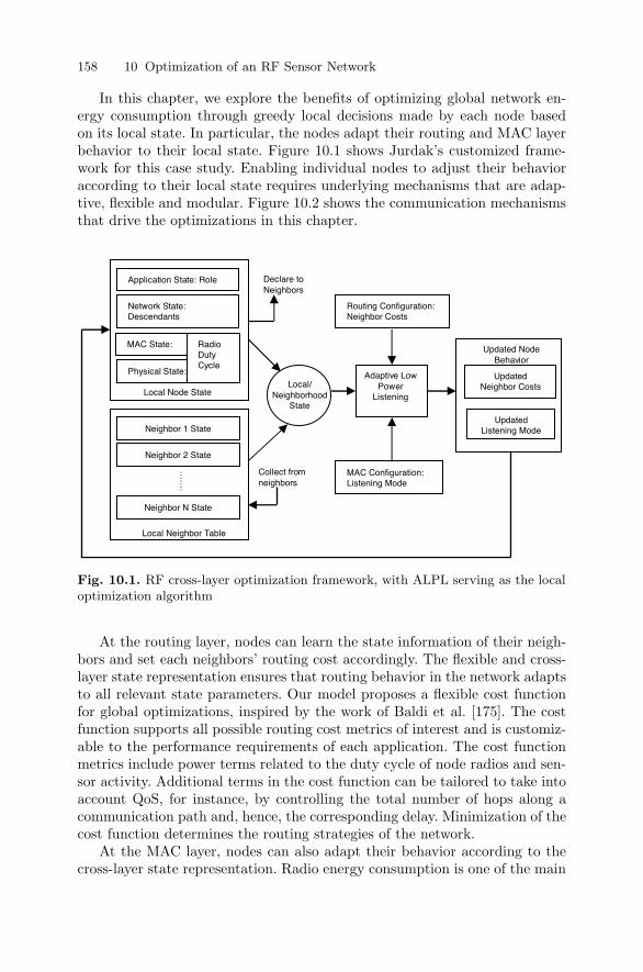
158 10 Optimization of an RF Sensor Network
In this chapter, we explore the benefits of optimizing global network en-ergy consumption through greedy local decisions made by each node basedon its local state. In particular, the nodes adapt their routing and MAC layerbehavior to their local state. Figure 10.1 shows Jurdak’s customized frame-work for this case study. Enabling individual nodes to adjust their behavioraccording to their local state requires underlying mechanisms that are adap-tive, flexible and modular. Figure 10.2 shows the communication mechanismsthat drive the optimizations in this chapter.
Application State: Role
Network State: Descendants
MAC State:
Physical State:
Radio Duty Cycle
Neighbor 1 State
Neighbor 2 State
Neighbor N State
Local Node State
.……
Local Neighbor Table
Collect from neighbors
Local/ Neighborhood
State
Declare to Neighbors
Routing Configuration: Neighbor Costs
MAC Configuration: Listening Mode
Updated Neighbor Costs
Updated Listening Mode
Adaptive Low Power
Listening
Updated Node Behavior
Fig. 10.1. RF cross-layer optimization framework, with ALPL serving as the localoptimization algorithm
At the routing layer, nodes can learn the state information of their neigh-bors and set each neighbors’ routing cost accordingly. The flexible and cross-layer state representation ensures that routing behavior in the network adaptsto all relevant state parameters. Our model proposes a flexible cost functionfor global optimizations, inspired by the work of Baldi et al. [175]. The costfunction supports all possible routing cost metrics of interest and is customiz-able to the performance requirements of each application. The cost functionmetrics include power terms related to the duty cycle of node radios and sen-sor activity. Additional terms in the cost function can be tailored to take intoaccount QoS, for instance, by controlling the total number of hops along acommunication path and, hence, the corresponding delay. Minimization of thecost function determines the routing strategies of the network.
At the MAC layer, nodes can also adapt their behavior according to thecross-layer state representation. Radio energy consumption is one of the main
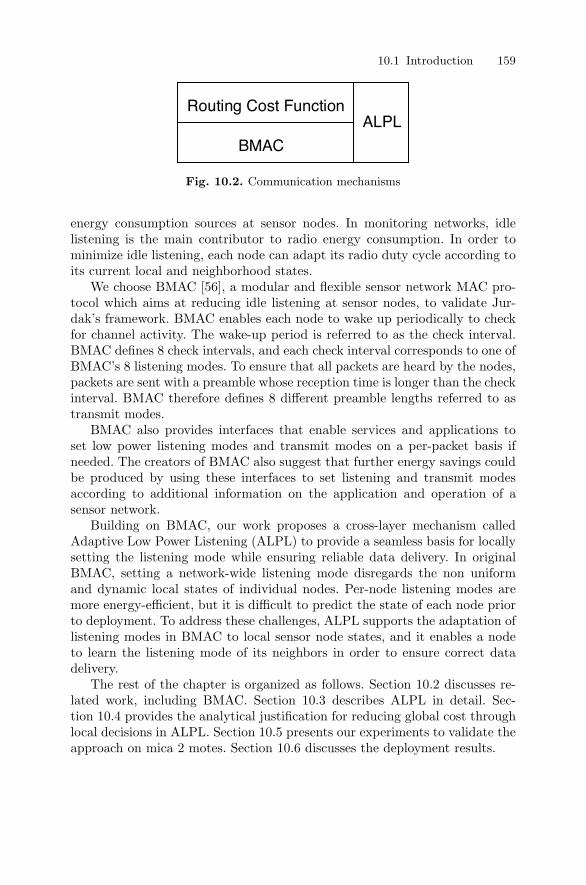
10.1 Introduction 159
Routing Cost Function
BMAC
ALPL
Fig. 10.2. Communication mechanisms
energy consumption sources at sensor nodes. In monitoring networks, idlelistening is the main contributor to radio energy consumption. In order tominimize idle listening, each node can adapt its radio duty cycle according toits current local and neighborhood states.
We choose BMAC [56], a modular and flexible sensor network MAC pro-tocol which aims at reducing idle listening at sensor nodes, to validate Jur-dak’s framework. BMAC enables each node to wake up periodically to checkfor channel activity. The wake-up period is referred to as the check interval.BMAC defines 8 check intervals, and each check interval corresponds to one ofBMAC’s 8 listening modes. To ensure that all packets are heard by the nodes,packets are sent with a preamble whose reception time is longer than the checkinterval. BMAC therefore defines 8 different preamble lengths referred to astransmit modes.
BMAC also provides interfaces that enable services and applications toset low power listening modes and transmit modes on a per-packet basis ifneeded. The creators of BMAC also suggest that further energy savings couldbe produced by using these interfaces to set listening and transmit modesaccording to additional information on the application and operation of asensor network.
Building on BMAC, our work proposes a cross-layer mechanism calledAdaptive Low Power Listening (ALPL) to provide a seamless basis for locallysetting the listening mode while ensuring reliable data delivery. In originalBMAC, setting a network-wide listening mode disregards the non uniformand dynamic local states of individual nodes. Per-node listening modes aremore energy-efficient, but it is difficult to predict the state of each node priorto deployment. To address these challenges, ALPL supports the adaptation oflistening modes in BMAC to local sensor node states, and it enables a nodeto learn the listening mode of its neighbors in order to ensure correct datadelivery.
The rest of the chapter is organized as follows. Section 10.2 discusses re-lated work, including BMAC. Section 10.3 describes ALPL in detail. Sec-tion 10.4 provides the analytical justification for reducing global cost throughlocal decisions in ALPL. Section 10.5 presents our experiments to validate theapproach on mica 2 motes. Section 10.6 discusses the deployment results.
160 10 Optimization of an RF Sensor Network
10.2 Related Work
This section surveys the related work in the literature. The discussion firstexamines existing approaches on cost optimization. The second part of thissection revisits approaches for providing energy efficiency at both the networkand data link layers.
10.2.1 Cost Optimization
Previous efforts [175, 176] have realized the need for optimizing global costin wireless networks, which determines the routing strategies of the net-work. Baldi et al. [175] develop a global cost function for wireless ultra wideband (UWB) radio networks, based on the cost of individual links. Their costfunction is additive and considers transmission power, link setup cost, inter-ference, delay and reliability. Mhatre et al. [176] optimize the hardware costof heterogeneous sensor networks with a lifetime constraint. Their work con-siders a network with 2 types of nodes, and attempts to determine both thenumber and position of each node to minimize overall hardware cost whilesatisfying the lifetime constraint. Jurdak’s customized framework focuses ondynamic cost optimization, so it disregards the hardware cost which is staticonce the network is deployed. The framework adopts a cost function similarto the function in [175] and customizes it for sensor networks through theintroduction of the composite metrics of data delivery and energy efficiencythat are central to most sensor network applications.
10.2.2 Energy Efficiency
In sensor networks, energy efficiency and load balancing are the primary met-rics of interest. Many protocols have been designed to provide energy-efficientbehavior at both the MAC layer [179,180] and the routing layer [181].
Routing Protocols
As indicated in Chapter 4, routing protocols are either proactive [182, 183]or reactive [184, 185]. Proactive protocols maintain network or neighborhoodrouting state tables at each node. Reactive protocols compute optimal routeson-demand. Proactive protocols are advantageous for networks that requirelimited mobility, low latency, or high throughput. In contrast, reactive proto-cols are suitable for high mobility, low throughput, high latency networks. Inthis chapter, we consider a typical stationary time-driven monitoring sensornetwork in which the periodic nature of data transmission fits well with peri-odic state exchanges in proactive routing protocols. As a result, we consider aproactive and periodic routing protocol in which nodes store the routing stateof their one-hop neighbors.
10.2 Related Work 161
Although many cost metrics have been proposed for routing in sensornetworks, we focus the discussion here on metrics for optimizing energy con-sumption. Previous work has examined energy optimizing routing strategies,where cost metrics include residual battery energy [186,187]. The residual bat-tery capacity strategy is intuitively valid, but the discharge of real batteriesbecomes nonlinear or unpredictable at a certain voltage level, which effectivelycancels battery considerations from routing decisions at some point during thedeployment [101]. In our work, we consider the radio, sensor, and processorduty cycles in the recent time window as the energy metric for routing. Webelieve that this metric is more expressive of each sensor node’s energy pro-file since it is independent of the battery technology and it does not rely onunpredictable battery discharge models.
MAC Protocols
At the MAC layer, idle listening constitutes a large portion of energy consump-tion because data is sent infrequently. This effect is even more pronounced inmonitoring sensor networks [188]. Thus, energy-efficient MAC protocol pro-posals have focused on minimizing idle listening at sensor nodes [56–58,189].
IEEE 802.15.4 [189] is a standard with physical and MAC layer specifica-tions for low rate, low power, short-range networks, including sensor networks.IEEE 802.15.4 specifies a plethora of functionality choices, many of which maynever be used. As a result, several researchers have proposed new MAC pro-tocols on top of the 802.15.4 PHY layer.
SMAC [57] is a heavyweight MAC protocol for sensor networks that re-lies on time synchronization and scheduling among nodes to enforce periodicsleep and listen schedules. SMAC reduces energy consumption and providesscalability at the cost of per-hop fairness, throughput, and latency. A morerecent version of SMAC [190] has introduced adaptive duty cycles by enablinga node to snoop on neighbors’ RTS and CTS messages in order to scheduleits own wake up time. Because nodes have to maintain neighbors’ schedules,SMAC is complex and not sufficiently scalable for large scale networks ofresource-limited nodes.
T-MAC [58] also proposes adaptive duty cycles to address the nonuniformtraffic patterns in sensor networks. T-MAC is similar to SMAC in its essence,but it introduces early sleeping to enable nodes that are scheduled to be activeto go into sleep mode if they are idle. T-MAC suffers from similar complexityand scaling problems of S-MAC, because it trades off a short active time forreduced adaptivity to changing network conditions.
The recent work by Polastre et al. proposes BMAC [56], a lightweight sen-sor network MAC protocol that aims at providing versatile medium accesswhile keeping the MAC functionality as simple as possible. Because it is anasynchronous protocol, BMAC eliminates the communication and processingoverhead for scheduling and synchronization, which reduces energy consump-tion. BMAC enables each node to wake up periodically to check for channel
162 10 Optimization of an RF Sensor Network
activity, where the wake-up period is referred to as the check interval. Po-lastre et al. analytically derive optimal check intervals based on the numberof neighbors of a node. In their experiments, they determine the maximumneighborhood size in the network, and they set the optimal check interval (orlistening mode) for that neighborhood size. The experimental results yieldsignificant energy savings for BMAC over previous protocols, such as SMAC.BMAC is also the standard MAC protocol in the communication stack ofTinyOS [191], the primary sensor network research platform.
As in T-MAC and SMAC, ALPL addresses the nonuniform node statesby adapting listening modes in BMAC to enable adaptive duty cycles. Wechoose BMAC because of its flexibility and scalability, which are two of ourmain design goals. Instead of proposing a new MAC protocol, this chapter’sfocus is designing a mechanism (namely ALPL) that enables each node toadapt its duty cycle based on flexible cross-layer node state representations.
10.3 Adaptive Low Power Listening
The general algorithm within Jurdak’s framework periodically runs the samethree basic steps for any network scenario:
1. Gather neighborhood state information
2. Perform local calculations on gathered state
3. Modify local configuration accordingly
The details of the algorithm and its implementation are highly dependenton the network scenario. As such, this section discusses the details of thealgorithm tailored for a monitoring sensor network application. We begin byintroducing the motivation for ALPL within the framework. Next, we describethe node interaction that enables nodes to set listening modes through ALPLand to exchange their state information. We subsequently describe the threestate representations that are considered in this chapter. Next, we explain howeach node uses its neighborhood state information to calculate the routing costof each neighbor through the cost function. Finally, we present the necessaryrouting protocol modifications to ensure correct data delivery with ALPL.
10.3.1 Adaptive Low Power Listening
Adaptive Low Power Listening [192, 193] is a cross-layer mechanism thatadapts the listening mode at each node according to its local state, whileensuring correct data delivery.
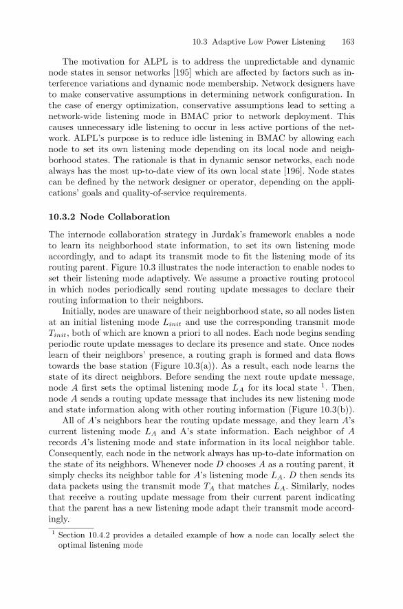
10.3 Adaptive Low Power Listening 163
The motivation for ALPL is to address the unpredictable and dynamicnode states in sensor networks [195] which are affected by factors such as in-terference variations and dynamic node membership. Network designers haveto make conservative assumptions in determining network configuration. Inthe case of energy optimization, conservative assumptions lead to setting anetwork-wide listening mode in BMAC prior to network deployment. Thiscauses unnecessary idle listening to occur in less active portions of the net-work. ALPL’s purpose is to reduce idle listening in BMAC by allowing eachnode to set its own listening mode depending on its local node and neigh-borhood states. The rationale is that in dynamic sensor networks, each nodealways has the most up-to-date view of its own local state [196]. Node statescan be defined by the network designer or operator, depending on the appli-cations’ goals and quality-of-service requirements.
10.3.2 Node Collaboration
The internode collaboration strategy in Jurdak’s framework enables a nodeto learn its neighborhood state information, to set its own listening modeaccordingly, and to adapt its transmit mode to fit the listening mode of itsrouting parent. Figure 10.3 illustrates the node interaction to enable nodes toset their listening mode adaptively. We assume a proactive routing protocolin which nodes periodically send routing update messages to declare theirrouting information to their neighbors.
Initially, nodes are unaware of their neighborhood state, so all nodes listenat an initial listening mode Linit and use the corresponding transmit modeTinit, both of which are known a priori to all nodes. Each node begins sendingperiodic route update messages to declare its presence and state. Once nodeslearn of their neighbors’ presence, a routing graph is formed and data flowstowards the base station (Figure 10.3(a)). As a result, each node learns thestate of its direct neighbors. Before sending the next route update message,node A first sets the optimal listening mode LA for its local state 1. Then,node A sends a routing update message that includes its new listening modeand state information along with other routing information (Figure 10.3(b)).
All of A’s neighbors hear the routing update message, and they learn A’scurrent listening mode LA and A’s state information. Each neighbor of Arecords A’s listening mode and state information in its local neighbor table.Consequently, each node in the network always has up-to-date information onthe state of its neighbors. Whenever node D chooses A as a routing parent, itsimply checks its neighbor table for A’s listening mode LA. D then sends itsdata packets using the transmit mode TA that matches LA. Similarly, nodesthat receive a routing update message from their current parent indicatingthat the parent has a new listening mode adapt their transmit mode accord-ingly.1 Section 10.4.2 provides a detailed example of how a node can locally select the
optimal listening mode
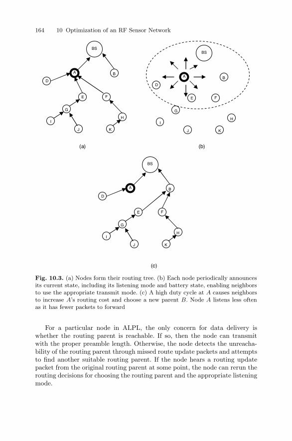
164 10 Optimization of an RF Sensor Network
H
H
G
H
(a) (b)
A
D
B
BS
E F
G
I
J K
A
D
B
BS
A
D
B
BS
E F
I
J K
E F
G
I
J K
(c)
Fig. 10.3. (a) Nodes form their routing tree. (b) Each node periodically announcesits current state, including its listening mode and battery state, enabling neighborsto use the appropriate transmit mode. (c) A high duty cycle at A causes neighborsto increase A’s routing cost and choose a new parent B. Node A listens less oftenas it has fewer packets to forward
For a particular node in ALPL, the only concern for data delivery iswhether the routing parent is reachable. If so, then the node can transmitwith the proper preamble length. Otherwise, the node detects the unreacha-bility of the routing parent through missed route update packets and attemptsto find another suitable routing parent. If the node hears a routing updatepacket from the original routing parent at some point, the node can rerun therouting decisions for choosing the routing parent and the appropriate listeningmode.
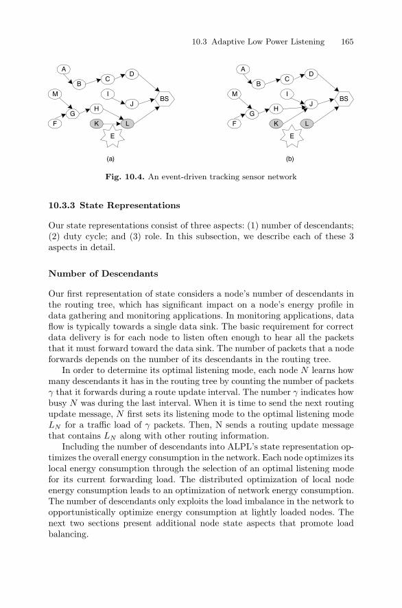
10.3 Adaptive Low Power Listening 165
AD
J
L
I
KF
C
H
B
G
MBS
E
AD
J
L
I
KF
C
H
B
G
MBS
E
(a) (b)
Fig. 10.4. An event-driven tracking sensor network
10.3.3 State Representations
Our state representations consist of three aspects: (1) number of descendants;(2) duty cycle; and (3) role. In this subsection, we describe each of these 3aspects in detail.
Number of Descendants
Our first representation of state considers a node’s number of descendants inthe routing tree, which has significant impact on a node’s energy profile indata gathering and monitoring applications. In monitoring applications, dataflow is typically towards a single data sink. The basic requirement for correctdata delivery is for each node to listen often enough to hear all the packetsthat it must forward toward the data sink. The number of packets that a nodeforwards depends on the number of its descendants in the routing tree.
In order to determine its optimal listening mode, each node N learns howmany descendants it has in the routing tree by counting the number of packetsγ that it forwards during a route update interval. The number γ indicates howbusy N was during the last interval. When it is time to send the next routingupdate message, N first sets its listening mode to the optimal listening modeLN for a traffic load of γ packets. Then, N sends a routing update messagethat contains LN along with other routing information.
Including the number of descendants into ALPL’s state representation op-timizes the overall energy consumption in the network. Each node optimizes itslocal energy consumption through the selection of an optimal listening modefor its current forwarding load. The distributed optimization of local nodeenergy consumption leads to an optimization of network energy consumption.The number of descendants only exploits the load imbalance in the network toopportunistically optimize energy consumption at lightly loaded nodes. Thenext two sections present additional node state aspects that promote loadbalancing.
166 10 Optimization of an RF Sensor Network
Duty Cycle
Our second state representation combines the number of descendants and thenode’s duty cycle. A high radio duty cycle indicates that the node’s radio hasbeen highly active up until the present point in time and vice versa. Giventhe inherently nonuniform energy consumption in sensor networks, enablingnodes to adapt their behavior according to their radio duty cycle can helpbalance the energy consumption in the network.
Sharing duty cycle information among nodes involves minimal overheadcommunication. Each node can piggyback its duty cycle value within its rout-ing update messages in order to declare its power state to neighbors. As aresult, nodes learn the radio duty cycles of all their one-hop neighbors andstore this information in their local neighbor table.
Including the radio duty cycle into ALPL’s state representation enableslocal load balancing of network traffic. Each node can consider and comparethe recent activity level of neighbor transceivers. Neighbors with a relativelyhigher radio duty cycle are penalized through higher routing cost, which di-verts traffic away from busier nodes to other nodes to achieve more uniformenergy consumption. The radio duty cycle promotes load balancing to theextent allowed by the routing graph. As long as the routing graph providesa node with more than one alternative for a routing parent, the radio dutycycle information contributes favorably to load balancing.
As an example, consider Figure 10.3 again. The routing tree in Fig-ure 10.3(a) puts most of the forwarding burden on node A. As a result, Adepletes its battery resources quicker than node B. In order to shift its for-warding load, A declares its high duty cycle to its neighbors, causing neighborsto increase A’s routing cost. This in turn causes most of A’s current childrento choose another parent whenever possible (Figure 10.3(c)). Having divertedmost of its forwarding load to node B, node A begins listening with a longercheck interval to reduce its listening energy consumption.
Role
The nonuniform state of sensor nodes also stems from the roles that the nodesmay take during deployment. The number of descendants is a routing aspectand it represents the present state of the node. The duty cycle is a physicaland MAC layer aspect that represents the past state of the node. The node’srole provides information on application functionality and represents its pro-jected state into the future. In the context of our energy optimization study,the node’s role can play a part in determining the node’s optimal listeningmode and neighbors’ routing costs. The rationale is to incorporate additionalknowledge about the expected power profile of a node’s role in optimal localdecisions.
In order to integrate role into network decisions, nodes should share theirrole status with their neighbors. Sharing role information among nodes in-volves minimal overhead communication. For example, in a network where
10.3 Adaptive Low Power Listening 167
nodes may take one of two roles, each node can include its role status withinits routing update messages through a single bit. As a result, nodes learn theroles of all their one-hop neighbors and store this information in their localneighbor table.
As in the case of radio duty cycles, including node roles into ALPL’s staterepresentation promotes local load balancing of network traffic. Each node canconsider and compare the recent sensing activity level of neighboring nodes.Thus, a node can divert traffic away from nodes with high sensing activ-ity, which contributes to load balancing. In homogeneous networks where allnodes behave the same, the role variable does not contribute to load balanc-ing. However, in event or query driven networks, certain nodes may assumemore active sensing roles during the deployment. In these cases, the energyconsumption for sensing becomes more significant and it should be consideredfor load balancing considerations.
Consider the network in Figure 10.4. While nodes are periodically sendingtheir data with period T , much of the forwarding load is focused at node L. Atsome point during the deployment, an event E occurs at the lower peripheryof the network. Nodes K and L detect event E, switch their role to tracker,and begin sensing and reporting data at T/2. The neighbors of K and L learnthat these 2 nodes are now tracker nodes and thereby increase the routing costof these 2 nodes. Figure 10.4(b) shows the resulting topology. Nodes K andH choose a new parent, node J , in order to avoid using the tracker node L asa forwarder. The topology in Figure 10.4(b) puts most of the forwarding loadon node J . The energy consumption resulting from the high forwarding loadof node J is balanced by the energy consumption for more frequent sensingand data reporting at node L.
10.3.4 Cost Function
Our primary platform for sensor network development is TinyOS [191], devel-oped at UC Berkeley. Within TinyOS, the standard routing protocol is calledMintRoute [197]. MintRoute is a proactive routing protocol in which nodessend periodic routing messages to declare their local states to their one-hopneighbors.
In all proactive routing protocols and particularly in MintRoute, each nodeperiodically selects its routing parent. Node N first selects the highest con-tender M in its neighbor table with the least routing cost at the current time.Next, N compares the cost of M with the cost of the current routing parentRP . N chooses M as its new parent only if:
Cmint(M) + ε < Cmint(RP ) (10.1)
where Cmint(Nj) is the routing cost of node Nj , and ε is the switching thresh-old that ensures that a node switches its routing parent only when there is anappreciable benefit in doing so.
168 10 Optimization of an RF Sensor Network
The original cost metric in MintRoute involves both hop count and linkquality. In particular, the cost metric assigns the link weight as the productof the reciprocal of the forward and backward link qualities, similar to theETX routing metric in Section 4.1.2. MintRoute then uses a shortest pathalgorithm for determining the best route to a destination.
The main purpose of integrating a shortest path algorithm with a linkquality metric is to maximize data delivery by choosing the shortest and mostreliable path to the base station. The shortest path algorithm reduces thenumber of reliable nodes involved in forwarding activity. Link quality reducesthe number of retransmissions by favoring more reliable links. The resultingalgorithm also implicitly enforces energy efficiency. Since Jurdak’s customizedframework aims at making routing decisions dependent on the node states, weintroduce additional cost metrics that are direct functions of the aspects thatconstitute node state. A discussion of further potential cost function metricsis available in Appendix A.
Duty Cycle Awareness
The number of descendants aspect is considered for setting local listeningmodes rather than setting neighbor costs, so this aspect does not require anexplicit routing cost metric. For the duty cycle aspect, we introduce the costmetric C(radio), which denotes how busy a particular neighbor’s radio isrelative to other neighboring nodes. Highly loaded nodes should have a higherrouting cost. Therefore, we express C(radio) for a neighbor Nj as:
C(radio) = εδj −
∑ki=0 δi/k√∑k
i=0 δ2i /k − (
∑ki=0 δi/k)2
(10.2)
where k is the number of neighbors in the node’s local neighbor table, andδi is the radio duty cycle of neighbor Ni. Equation 10.2 compares the radioduty cycle of neighbor Nj to the average duty cycle in the neighborhood andnormalizes the difference. The normalized difference determines the extent ofstatistical deviation of the radio activity of Nj among all the nodes in theneighborhood.
Role Awareness
The duty cycle is a sufficient indicator of energy profiles in cases where thenodes all have the same sensing and processing patterns throughout the life-time of the network. In many event-driven or demand-driven sensor networks,some nodes change their application behavior, such as the sensing frequencyor buffering strategy, based on events in the network. Such cases require theinclusion of information on the current roles of nodes in routing decisions.
The actual cost dependance on the node’s role is highly application-specific. In this chapter, we consider an event-driven network that specifies
10.3 Adaptive Low Power Listening 169
that nodes can have one of two sensing frequencies f1 and f2, where f2 isdouble f1. A node uses the following equation to evaluate the sensing cost ofa neighbor Nj :
C(sensing) =
⎧⎪⎨⎪⎩
εθj−
∑k
i=0θi/k√∑k
i=0θ2
i/k−(
∑k
i=0θi/k)2
θj = 1
0 θj = 0
(10.3)
where k is the number of neighbors in the node’s local table. θi is a Booleanvariable that takes the value of 1 if Ni is sensing data at frequency f2 (trackernode) and takes the value of 0 if Ni is sensing data at frequency f1. Equa-tion 10.3 compares the sensing activity of neighbor Nj to the average sensingactivity in the neighborhood and normalizes the difference. The normalizeddifference determines the extent of statistical deviation of the sensing activityof Nj among all the nodes in the neighborhood.
Overall Cost Metric
The overall routing cost should strike a balance between the need for correctand timely data delivery on one hand and uniform energy cost on the other.Furthermore, C(radio) and C(sensing) should play a role in determining therouting parent only if the node M is at the same or at a lower level than thecurrent routing parent RP .
Therefore, the new overall cost of a neighbor includes the original MintRoutecost of quality and hops, as well as the power cost according to the followingequation:
C(M) ={
Cmint(M) + αC(radio) + βC(sensing) H(M) ≤ H(RP )Cmint(M) H(M) > H(RP )
(10.4)where α and β are constants representing the weights of C(radio) andC(sensing) respectively. H(M) indicates the hop count of node M from thebase station. With the new cost definition, neighbors with higher energy con-sumption (due either to radio duty cycle or to increased sensing activity) havea higher routing cost, and they are less likely to be chosen as forwarders.
Global Network Cost
The global network cost in Jurdak’s customized framework is the sum of thecosts of individual nodes [175]:
NC =∑N
C(N) (10.5)
Since optimizing NC is not feasible, each node selects its routing parent asthe node with the least routing cost C(N).
170 10 Optimization of an RF Sensor Network
10.3.5 Routing Modifications
Enabling each node to set its own listening mode adapts MAC protocol behav-ior to the node’s state. The MAC protocol adaptation should be accompaniedwith routing protocol adaptation in order to maximize performance gains.
The concept of adaptive listening modes raises the possibility that somenodes may not hear the packets sent by their neighbors because of mismatchedpreamble lengths and check intervals. For example, if node A sends a packetwith a short preamble to its parent B, one of node A’s neighbors C that islistening infrequently may miss node A’s packet. This situation does not affectdata delivery, since it is only necessary for A’s parent B to hear the packet.Missing a routing update packet is more detrimental, since routing packetshold important information on neighborhood routing state changes.
We implement modifications to MintRoute to address missed routing up-date packets. A central issue in designing ALPL is to ensure that symmetriclistening modes do not affect maintaining an up-to-date neighborhood viewat each node. Achieving this goal requires that nodes always hear the routingupdate packets of their neighbors. Thus, ALPL specifies that nodes alwayssend their routing update packets with the longest preamble, so that a neigh-bor in any listening mode can hear the update packets. Secondly, MintRoutedetermines quality as the percentage of data packets correctly received from aneighbor. The example above on missed data packets causes the quality met-ric in MintRoute to drop. Consequently, we modify MintRoute so that nodesonly snoop on periodic routing updates instead of data packets to determinethe link quality to their neighbors. Monitoring route update packets for deter-mining link quality ensures that asymmetric listening modes at neighboringnodes have no detrimental effect on link quality, because all routing updatepackets are sent with the longest preamble.
10.4 Qualitative Analysis
This section presents the analytical basis for using greedy local decisions toreduce global network energy consumption. We assume that the sensor nodescollect sensor data and transmit the data in a packet once in every periodT . The following equation governs the energy consumption E at a sensornode [56]:
E = Et + Er + Ed + Elisten + Esleep (10.6)
where Et is the energy consumed on transmissions during time T , Er is theenergy consumed for packet reception during time T , Ed is the energy con-sumption to collect sensor values, Elisten is the energy consumed for checkingthe channel for activity, and Esleep is the energy consumed while the nodeis asleep. The quantitative expressions for each energy component are givenin [56]. We limit the discussion here to the qualitative aspects that are relevantto ALPL.
10.4 Qualitative Analysis 171
In monitoring and data gathering applications, the sampling period T istypically in the order of minutes. Therefore, each node collects sensor data,transmits packets, and receives packets once every few minutes. On the otherhand, nodes wake up to monitor the channel for activity much more frequently,for instance once every several milliseconds. Thus, idle listening on the channelhas a profound effect on the average power consumption, so reducing idlelistening yields significant energy savings.
10.4.1 Topology
The aim of the number of descendants metric is to minimize the energy con-sumption in the network through local optimization decisions. Each node canoptimize its own consumption E locally by selecting its own optimal listeningmode while maintaining correct and timely data delivery. Minimizing E on aper-node basis reduces the overall network energy consumption and builds onthe following observations about Equation 10.6:
1. Ed and Esleep are not significant factors in determining optimal listeningmode in a homogeneous monitoring network. Ed is equal for all nodes.Esleep is at least an order of magnitude smaller than the other terms inEquation 10.6, so it has a negligible effect on E.
2. Et and Er depend on the node’s position in the logical topology. If a nodeis a leaf in the routing tree, it has fewer packets to forward.
3. The listening mode N determines Elisten. It also determines the preamblelength for packets that are received at N . Consequently, the listening modeat node N affects Er at N and Et at N ’s children.
For example, a more frequent listening mode at N increases Elisten anddecreases Er at N . Elisten increases because N wakes up more frequently tocheck for channel activity, and Er decreases because the frequent listeningenables N ’s neighbors to send their packets to N with shorter preambles,thereby reducing packet reception time at N .
Similarly, the listening mode of N affects Et at the children ci of N .A more frequent listening mode at N enables ci to send its packets withshorter preambles, thus reducing Eti
. Through similar reasoning, less frequentlistening at N forces ci to send packets with long preamble and consume moreenergy for packet transmissions.
These dependencies further support the need for setting per-node listeningmodes. In practice, each node locally computes Et, Ed, and Esleep and thenselects the listening mode that provides the combination of Elisten and Er
that yields the lowest energy consumption E.ALPL builds on the need to reduce idle listening and to balance energy
consumption. ALPL’s most basic state representation only considers num-ber of descendants in the routing tree, which yields energy savings at nodeswith few descendants. We now consider a case study analysis to illustrate thebenefits, scalability and shortcomings of this most basic form of ALPL.
172 10 Optimization of an RF Sensor Network
10.4.2 Case Study
To analyze the tradeoffs involved in ALPL and to compare the energy con-sumption of ALPL and BMAC, we consider a case study of a static 127-nodenetwork with a binary tree topology. Although the topology of an actual sen-sor network can be both irregular and transient according to environmentalconditions as well as location, this case study serves the purpose of validatingthe analytical basis and the scalability of ALPL. In the next section, we per-form experiments with actual sensor nodes to further validate our model ina more dynamic and realistic scenario. Our analysis for this network assumesthat the sensor nodes sense the environment and send their data to the basestation once every 2 minutes.
In their evaluation of BMAC, Polastre et al. use the following method forassigning a listening mode that favors the busiest node to improve networklifetime:
• Compute the expected number of descendants of the busiest node in thenetwork
• Set the network-wide listening mode to favor the busiest node
Since the busiest node in the network has the largest forwarding load, thismethod for setting listening mode typically means that all the nodes in thenetwork use the higher duty cycle setting which suits the busy node. Thisgives rise to one of the motivations of ALPL: to enable nodes that are not asbusy to choose their appropriate duty cycle in a decentralized manner.
Table 10.1 compares the check interval between network-wide listeningmodes (plain BMAC) and ALPL at each level in the 127-node binary treenetwork. In plain BMAC, the check interval is initially set to 10 ms for allthe nodes in order to accommodate the forwarding load of the busiest node.In ALPL, the busiest node (the node at level 1) selects the same listeningmode as BMAC nodes, and the remaining nodes select their own listeningmodes based on their topology position. The following example illustrates thelistening mode selection process in ALPL.
We consider how a level 2 node in the 127-node binary tree selects itsoptimal check interval in ALPL. A level 2 node sends 63 data packets eachupdate period, where 1 packet is locally generated and the rest are forwardedpackets from its descendants. The level 2 node also uses a preamble lengthof 28 bytes in order to match its parent’s check interval of 10 ms. The re-sulting ALPL energy consumption Et during an update period for a level 2node is 0.1006 Joules. Using the fact that it receives 62 data packets fromits descendants each update period, the level 2 node then computes its recep-tion energy consumption Er for each of the 8 possible check intervals. It alsocomputes Elisten and Esleep for each check interval. Finally, the level 2 nodeselects a check interval of 20 ms, with a reception energy consumption Er of0.1509 Joules and a listening energy consumption Elisten of 0.1038 Joules, as
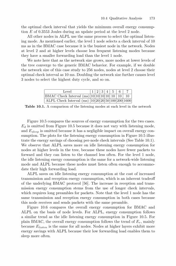
10.4 Qualitative Analysis 173
the optimal check interval that yields the minimum overall energy consump-tion E of 0.3553 Joules during an update period at the level 2 node.
All other nodes in ALPL use the same process to select the optimal listen-ing mode. As mentioned earlier, the level 1 node selects a check interval of 10ms as in the BMAC case because it is the busiest node in the network. Nodesat level 2 and at higher levels choose less frequent listening modes becausethey have a smaller forwarding load than the level 1 node.
We note here that as the network size grows, more nodes at lower levels ofthe tree converge to the generic BMAC behavior. For example, if we doublethe network size of this case study to 256 nodes, nodes at level 2 choose theiroptimal check interval as 10 ms. Doubling the network size further causes level3 nodes to select the highest duty cycle, and so on.
Level 1 2 3 4 5 6 7
BMAC Check Interval (ms) 10 10 10 10 10 10 10
ALPL Check Interval (ms) 10 20 20 50 100 200 1600
Table 10.1. A comparison of the listening modes at each level in the network
Figure 10.5 compares the sources of energy consumption for the two cases.Ed is omitted from Figure 10.5 because it does not vary with listening mode,and Esleep is omitted because it has a negligible impact on overall energy con-sumption. The plots for the listening energy consumption in Figure 10.5 illus-trate the energy savings of choosing per-node check intervals (See Table 10.1).We observe that ALPL saves more on idle listening energy consumption fornodes at higher levels in the tree, because these nodes have fewer packets toforward and they can listen to the channel less often. For the level 1 node,the idle listening energy consumption is the same for a network-wide listeningmode and ALPL because these nodes must listen often enough to accommo-date their high forwarding load.
ALPL saves on idle listening energy consumption at the cost of increasedtransmission and reception energy consumption, which is an inherent tradeoffof the underlying BMAC protocol [56]. The increase in reception and trans-mission energy consumption stems from the use of longer check intervals,which requires long preambles for packets. Note that the level 1 node has thesame transmission and reception energy consumption in both cases becausethis node receives and sends packets with the same preamble.
Figure 10.6 compares the overall energy consumption for BMAC andALPL on the basis of node levels. For ALPL, energy consumption followsa similar trend as the idle listening energy consumption in Figure 10.5. Forplain BMAC, the overall energy consumption follows the trend of Er, mainlybecause Elisten is the same for all nodes. Nodes at higher layers exhibit moreenergy savings with ALPL because their low forwarding load enables them tosleep more often.
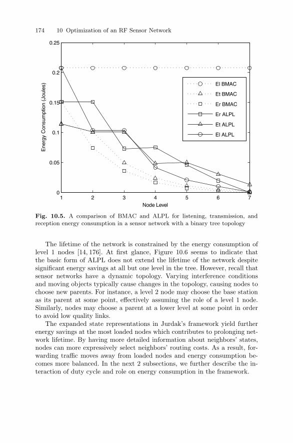
174 10 Optimization of an RF Sensor Network
1 2 3 4 5 6 70
0.05
0.1
0.15
0.2
0.25
Node Level
Ene
rgy
Con
sum
ptio
n (J
oule
s) El BMAC
Et BMAC
Er BMAC
Er ALPL
Et ALPL
El ALPL
Fig. 10.5. A comparison of BMAC and ALPL for listening, transmission, andreception energy consumption in a sensor network with a binary tree topology
The lifetime of the network is constrained by the energy consumption oflevel 1 nodes [14, 176]. At first glance, Figure 10.6 seems to indicate thatthe basic form of ALPL does not extend the lifetime of the network despitesignificant energy savings at all but one level in the tree. However, recall thatsensor networks have a dynamic topology. Varying interference conditionsand moving objects typically cause changes in the topology, causing nodes tochoose new parents. For instance, a level 2 node may choose the base stationas its parent at some point, effectively assuming the role of a level 1 node.Similarly, nodes may choose a parent at a lower level at some point in orderto avoid low quality links.
The expanded state representations in Jurdak’s framework yield furtherenergy savings at the most loaded nodes which contributes to prolonging net-work lifetime. By having more detailed information about neighbors’ states,nodes can more expressively select neighbors’ routing costs. As a result, for-warding traffic moves away from loaded nodes and energy consumption be-comes more balanced. In the next 2 subsections, we further describe the in-teraction of duty cycle and role on energy consumption in the framework.
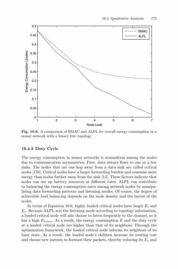
10.4 Qualitative Analysis 175
1 2 3 4 5 6 70
0.05
0.1
0.15
0.2
0.25
0.3
0.35
0.4
0.45
0.5
Node Level
Ene
rgy
Con
sum
ptio
n (J
oule
s)
BMAC
ALPL
Fig. 10.6. A comparison of BMAC and ALPL for overall energy consumption in asensor network with a binary tree topology
10.4.3 Duty Cycle
The energy consumption in sensor networks is nonuniform among the nodesdue to communication asymmetries. First, data always flows to one or a fewsinks. The nodes that are one hop away from a data sink are called criticalnodes [176]. Critical nodes have a larger forwarding burden and consume moreenergy than nodes further away from the sink [14]. These factors indicate thatnodes can use up battery resources at different rates. ALPL can contributeto balancing the energy consumption rates among network nodes by manipu-lating data forwarding patterns and listening modes. Of course, the degree ofachievable load balancing depends on the node density and the layout of thenodes.
In terms of Equation 10.6, highly loaded critical nodes have larger Et andEr. Because ALPL sets the listening mode according to topology information,a loaded critical node will also choose to listen frequently to the channel, so ithas a high Elisten. As a result, the energy consumption E and the duty cycleat a loaded critical node are higher than that of its neighbors. Through theoptimization framework, the loaded critical node informs its neighbors of itsbusy state. As a result, the loaded node’s children increase its routing costand choose new parents to forward their packets, thereby reducing its Er and
176 10 Optimization of an RF Sensor Network
Et at the loaded critical node. The loaded critical node then switches to alistening mode with a longer check interval to reduce Elisten. The reductionsin Er, Et, and Elisten cause the overall energy consumption E at the criticalnode to drop significantly.
10.4.4 Role
In applications where nodes may dynamically select different roles, the sensingenergy consumption Ed may become a significant player in determining thenode’s energy consumption relative to its neighbors. For instance, suppose theoccurrence of a particular event causes some nodes in the network to doubletheir sampling frequency in order to better track the event. The increasedsampling frequency at these nodes increases the sensing energy consumptionEd and it also increases Et because the node sends packets more frequently toreport the more frequent sensed data. The increase in Et falls within the radioduty cycle value so it does not cause any distortion for energy balancing. Themore appreciable increase in Ed has no explicit effect on the radio duty cycleat the node, but it can cause energy imbalances in the network. Including thesensing energy consumption Ed in routing and MAC decisions remedies thisproblem and maintains a balance in overall energy consumption E among thenodes.
10.5 Deployment Results
In this section, we investigate the impact of local state-driven optimizationson a test-bed of sensor nodes deployed in our laboratory. The sensor nodesin our experiments consist of 14 mica 2 motes from Crossbow [7]. Our im-plementation of ALPL is in NesC [199], a component-oriented variant of Ccustomized for networked embedded systems and built into TinyOS.
The nodes are placed at random positions in the laboratory and the basestation is placed near one of the walls of the room. We reduce the transmitpower of nodes to limit their radio range, enabling multihop communication.The aim of the experiments is twofold: (1) to assess the effect of state-drivenoptimizations on the global network energy consumption; and (2) to evaluatethe local node energy consumption and energy balancing benefits for state-driven optimizations.
We adopt the method suggested by [56] for computing energy consump-tion. The underlying BMAC design includes several radio states, includingactive and sleep states. The average current draw for each radio state is fixed.The method employs a counter that keeps track of the time that the radiospends in each power state. Having the current draw and time spent in eachstate, each node can continually compute its aggregated energy consumptionso far. The energy consumption results shown for our deployments represent
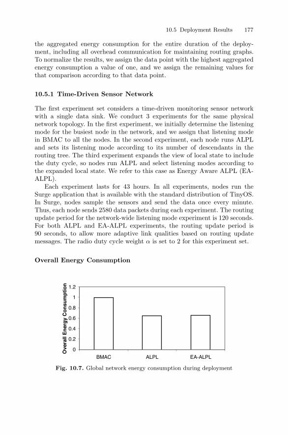
10.5 Deployment Results 177
the aggregated energy consumption for the entire duration of the deploy-ment, including all overhead communication for maintaining routing graphs.To normalize the results, we assign the data point with the highest aggregatedenergy consumption a value of one, and we assign the remaining values forthat comparison according to that data point.
10.5.1 Time-Driven Sensor Network
The first experiment set considers a time-driven monitoring sensor networkwith a single data sink. We conduct 3 experiments for the same physicalnetwork topology. In the first experiment, we initially determine the listeningmode for the busiest node in the network, and we assign that listening modein BMAC to all the nodes. In the second experiment, each node runs ALPLand sets its listening mode according to its number of descendants in therouting tree. The third experiment expands the view of local state to includethe duty cycle, so nodes run ALPL and select listening modes according tothe expanded local state. We refer to this case as Energy Aware ALPL (EA-ALPL).
Each experiment lasts for 43 hours. In all experiments, nodes run theSurge application that is available with the standard distribution of TinyOS.In Surge, nodes sample the sensors and send the data once every minute.Thus, each node sends 2580 data packets during each experiment. The routingupdate period for the network-wide listening mode experiment is 120 seconds.For both ALPL and EA-ALPL experiments, the routing update period is90 seconds, to allow more adaptive link qualities based on routing updatemessages. The radio duty cycle weight α is set to 2 for this experiment set.
Overall Energy Consumption
0
0.2
0.4
0.6
0.8
1
1.2
BMAC ALPL EA-ALPL
Ove
rall
En
erg
y C
on
sum
pti
on
Fig. 10.7. Global network energy consumption during deployment
178 10 Optimization of an RF Sensor Network
The average data yield for BMAC, ALPL, and EA-ALPL is about 98.5%.Because the data yield is the same with or without state-driven optimizations,we focus our analysis here on energy consumption issues.
Figure 10.7 plots the average global network energy consumption forBMAC, ALPL, and EA-ALPL. Both ALPL and EA-ALPL reduce globalenergy consumption by about 35% on average during the deployment. Thereduction in global energy consumption stems from the optimal local deci-sions at each node. In particular, the number of descendants variable is themain contributor for the reductions in energy consumption, as the next sub-section reveals in more detail. This reduction also confirms the benefits ofgreedy local decisions in reducing overall network energy consumption.
The global energy consumption for ALPL and EA-ALPL experiments isalmost the same with a slight difference of 1%. The main distinction betweenALPL and EA-ALPL is in the distribution of the energy consumption amongnetwork nodes rather than in the aggregated energy consumption. The re-mainder of this subsection sheds more light on the issue of individual nodeenergy consumption that drives the global energy consumption reductions ofALPL and EA-ALPL and the details behind the load balancing benefits ofEA-ALPL.
Local Energy Consumption
We now turn our attention to local energy consumption at each node. We col-lect node statistics by piggybacking node status information into data packet.Each arriving data packet for a node provides one data point regarding nodestatus. Recall that during each 43 hour experiment, each node sends 2580data packets, yielding 2580 data points for each node.
Figure 10.8 shows the average check interval of each node in the BMAC,ALPL and EA-ALPL deployment experiments, with the error bars indicatingthe 99% confidence interval. In plain BMAC, all nodes use a check interval of20 ms. Nodes using ALPL or EA-ALPL can choose one of four check intervals:20 ms, 50 ms, 100 ms, or 200ms. In both ALPL and EA-ALPL, the averagecheck intervals of all nodes are longer than in BMAC, so all nodes save onidle listening energy consumption.
EA-ALPL yields a more balanced spread of check intervals among nodesthan ALPL or BMAC. The nodes with the lowest average check interval inALPL, such as nodes 1 and 8, have a higher average check interval with EA-ALPL. Similarly, some of the nodes with the highest average check intervalsin ALPL have lower check intervals in EA-ALPL. The balancing out of aver-age check intervals yields more balanced energy consumption among networknodes.
The narrow 99% confidence interval for all nodes in the ALPL and EA-ALPL experiments indicates the stability of this approach in the long-termexperiments. We also note that busier nodes with the smaller average checkinterval had slightly less stable check intervals compared to other nodes, due to
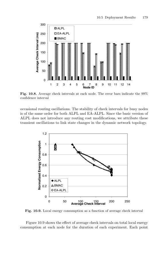
10.5 Deployment Results 179
0
50
100
150
200
250
300
1 2 3 4 5 6 7 8 9 10 11 12 14Node ID
Ave
rag
e C
hec
k In
terv
al (
ms)
ALPL
EA-ALPL
BMAC
Fig. 10.8. Average check intervals at each node. The error bars indicate the 99%confidence interval
occasional routing oscillations. The stability of check intervals for busy nodesis of the same order for both ALPL and EA-ALPL. Since the basic version ofALPL does not introduce any routing cost modifications, we attribute thesetransient oscillations to link state changes in the dynamic network topology.
0
0.2
0.4
0.6
0.8
1
1.2
0 50 100 150 200 250Average Check Interval
No
rmal
ized
En
erg
y C
on
sum
ptio
n
ALPL
BMAC
EA-ALPL
Fig. 10.9. Local energy consumption as a function of average check interval
Figure 10.9 shows the effect of average check intervals on total local energyconsumption at each node for the duration of each experiment. Each point
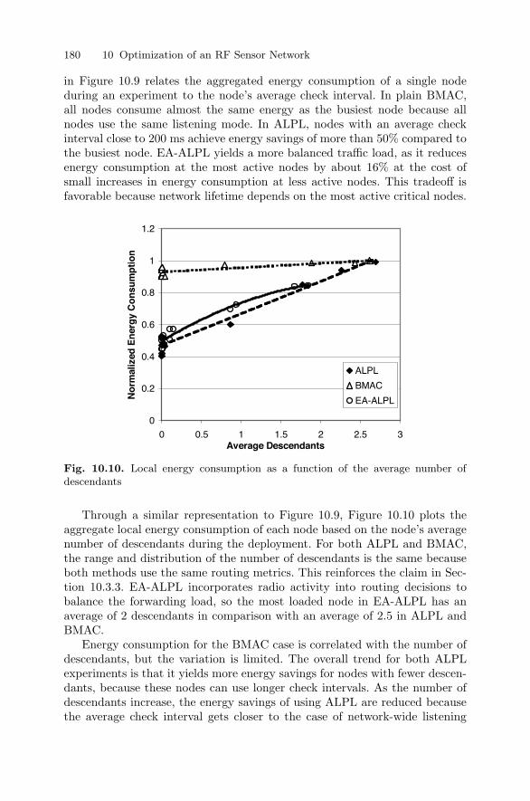
180 10 Optimization of an RF Sensor Network
in Figure 10.9 relates the aggregated energy consumption of a single nodeduring an experiment to the node’s average check interval. In plain BMAC,all nodes consume almost the same energy as the busiest node because allnodes use the same listening mode. In ALPL, nodes with an average checkinterval close to 200 ms achieve energy savings of more than 50% compared tothe busiest node. EA-ALPL yields a more balanced traffic load, as it reducesenergy consumption at the most active nodes by about 16% at the cost ofsmall increases in energy consumption at less active nodes. This tradeoff isfavorable because network lifetime depends on the most active critical nodes.
0
0.2
0.4
0.6
0.8
1
1.2
0 0.5 1 1.5 2 2.5 3Average Descendants
No
rmal
ized
En
erg
y C
on
sum
pti
on
ALPL
BMAC
EA-ALPL
Fig. 10.10. Local energy consumption as a function of the average number ofdescendants
Through a similar representation to Figure 10.9, Figure 10.10 plots theaggregate local energy consumption of each node based on the node’s averagenumber of descendants during the deployment. For both ALPL and BMAC,the range and distribution of the number of descendants is the same becauseboth methods use the same routing metrics. This reinforces the claim in Sec-tion 10.3.3. EA-ALPL incorporates radio activity into routing decisions tobalance the forwarding load, so the most loaded node in EA-ALPL has anaverage of 2 descendants in comparison with an average of 2.5 in ALPL andBMAC.
Energy consumption for the BMAC case is correlated with the number ofdescendants, but the variation is limited. The overall trend for both ALPLexperiments is that it yields more energy savings for nodes with fewer descen-dants, because these nodes can use longer check intervals. As the number ofdescendants increase, the energy savings of using ALPL are reduced becausethe average check interval gets closer to the case of network-wide listening
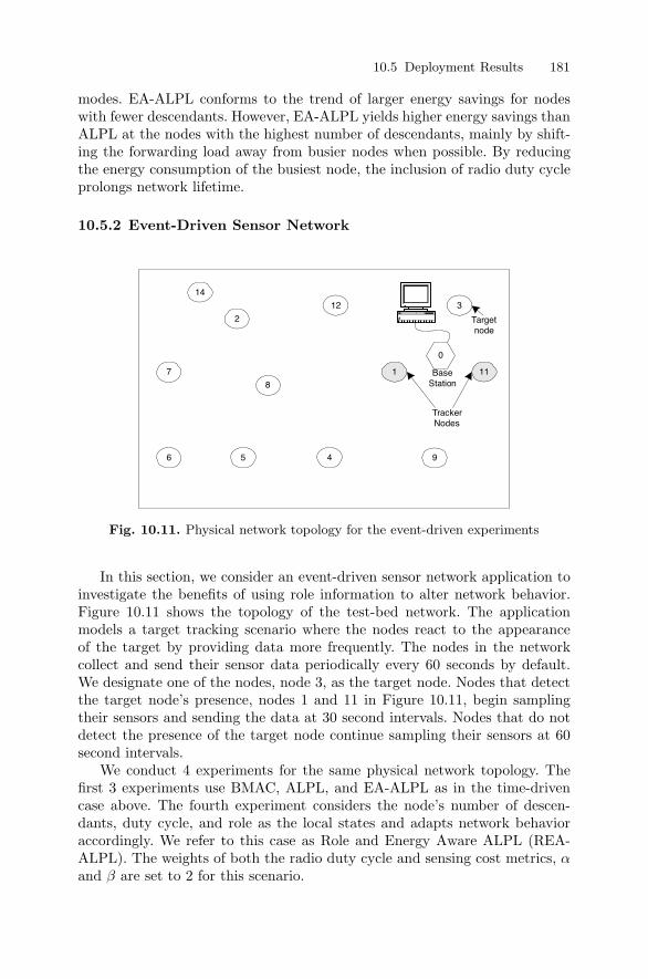
10.5 Deployment Results 181
modes. EA-ALPL conforms to the trend of larger energy savings for nodeswith fewer descendants. However, EA-ALPL yields higher energy savings thanALPL at the nodes with the highest number of descendants, mainly by shift-ing the forwarding load away from busier nodes when possible. By reducingthe energy consumption of the busiest node, the inclusion of radio duty cycleprolongs network lifetime.
10.5.2 Event-Driven Sensor Network
BaseStation
1 11
3
0
94
12
8
2
5
14
7
6
TrackerNodes
Targetnode
Fig. 10.11. Physical network topology for the event-driven experiments
In this section, we consider an event-driven sensor network application toinvestigate the benefits of using role information to alter network behavior.Figure 10.11 shows the topology of the test-bed network. The applicationmodels a target tracking scenario where the nodes react to the appearanceof the target by providing data more frequently. The nodes in the networkcollect and send their sensor data periodically every 60 seconds by default.We designate one of the nodes, node 3, as the target node. Nodes that detectthe target node’s presence, nodes 1 and 11 in Figure 10.11, begin samplingtheir sensors and sending the data at 30 second intervals. Nodes that do notdetect the presence of the target node continue sampling their sensors at 60second intervals.
We conduct 4 experiments for the same physical network topology. Thefirst 3 experiments use BMAC, ALPL, and EA-ALPL as in the time-drivencase above. The fourth experiment considers the node’s number of descen-dants, duty cycle, and role as the local states and adapts network behavioraccordingly. We refer to this case as Role and Energy Aware ALPL (REA-ALPL). The weights of both the radio duty cycle and sensing cost metrics, αand β are set to 2 for this scenario.

182 10 Optimization of an RF Sensor Network
0
0.2
0.4
0.6
0.8
1
1.2
BMAC ALPL EA-ALPL REA-ALPL
Ove
rall
En
erg
y C
on
sum
pti
on
Fig. 10.12. Global network energy consumption during deployment
Global Energy Consumption
The average data yield for BMAC, ALPL, EA-ALPL, and REA-ALPL re-mains at 98.5%. As in the time-driven case, data delivery rate does not dropwhen using Jurdak’s optimization framework.
Figure 10.12 plots the average global network energy consumption forBMAC, ALPL, EA-ALPL, and REA-ALPL. All three state representationsin ALPL yield almost the same overall energy consumption, since they allinclude the number of descendants variable, which is the main contributor toreduction of energy consumption. ALPL reduces the overall network energyconsumption by 21% over the BMAC case for this event-driven network. Thereductions in global energy consumption are lower than the time-driven net-work case because the sensing energy consumption constitutes a larger portionof overall energy consumption in the event-driven case.
Local Energy Consumption
We now turn our attention to the local energy consumption at each node.Before presenting the local energy consumption results, we note that the goalof this analysis is to illustrate how the addition of the role aspect contributesto load balancing, leading to a longer network lifetime. Ideally, all nodes woulddeplete their batteries at about the same time. In this experiment, the goalis to explore the extent to which nodes can recognize the increased sensingactivity of the tracker nodes 1 and 11 in order to avoid these nodes in routingdecisions.
We first examine the average check interval for each node during the de-ployment. Figure 10.13 plots the average check interval of each node for theduration of each of the three ALPL experiments. We omit the constant BMACcheck interval from the figure for presentation clarity. In the ALPL experi-ment, the tracker node with an ID of 1 is the busiest node with a checkinterval of 43 ms. By including radio duty cycle information, EA-ALPL shifts
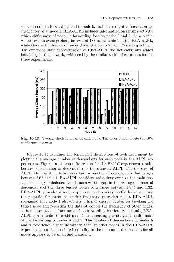
10.5 Deployment Results 183
some of node 1’s forwarding load to node 9, enabling a slightly longer averagecheck interval at node 1. REA-ALPL includes information on sensing activity,which shifts most of node 1’s forwarding load to nodes 8 and 9. As a result,we observe an average check interval of 183 ms at node 1 in the REA-ALPL,while the check intervals of nodes 8 and 9 drop to 51 and 75 ms respectively.The expanded state representation of REA-ALPL did not cause any addedinstability in the network, evidenced by the similar width of error bars for thethree experiments.
0
50
100
150
200
250
300
1 2 3 4 5 6 7 8 9 10 11 12 14Node ID
Ave
rag
e C
hec
k In
terv
al (
ms)
ALPL
EA-ALPL
REA-ALPL
Fig. 10.13. Average check intervals at each node. The error bars indicate the 99%confidence intervals
Figure 10.14 examines the topological distinctions of each experiment byplotting the average number of descendants for each node in the ALPL ex-periments. Figure 10.14 omits the results for the BMAC experiment resultsbecause the number of descendants is the same as ALPL. For the case ofALPL, the top three forwarders have a number of descendants that rangesbetween 2.62 and 1.1. EA-ALPL considers radio duty cycle as the main rea-son for energy imbalance, which narrows the gap in the average number ofdescendants of the three busiest nodes to a range between 1.875 and 1.32.REA-ALPL provides a more expressive node energy profile by consideringthe potential for increased sensing frequency at tracker nodes. REA-ALPLrecognizes that node 1 already has a higher energy burden for tracking thetarget node and reporting the data at double the frequency of other nodes,so it relieves node 1 from most of its forwarding burden. As a result, REA-ALPL forces nodes to avoid node 1 as a routing parent, which shifts mostof the forwarding to nodes 8 and 9. The number of descendants at nodes 8and 9 experience higher instability than at other nodes in the REA-ALPLexperiment, but the absolute instability in the number of descendants for allnodes appears to be small and transient.
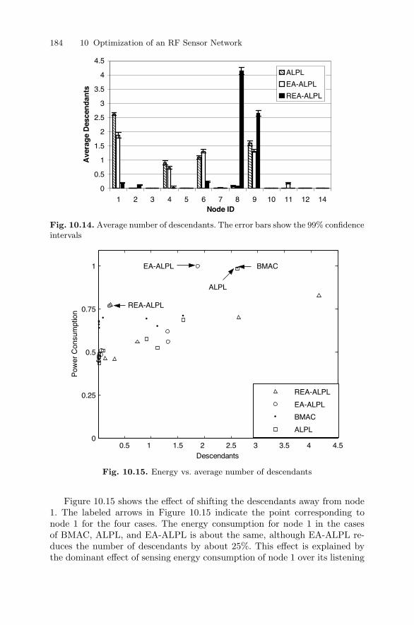
184 10 Optimization of an RF Sensor Network
0
0.5
1
1.5
2
2.5
3
3.5
4
4.5
1 2 3 4 5 6 7 8 9 10 11 12 14Node ID
Ave
rag
e D
esce
nd
ants
ALPL
EA-ALPL
REA-ALPL
Fig. 10.14. Average number of descendants. The error bars show the 99% confidenceintervals
0.5 1 1.5 2 2.5 3 3.5 4 4.50
0.25
0.5
0.75
1
Descendants
Pow
er C
onsu
mpt
ion
REA-ALPL
EA-ALPL BMAC
ALPL
REA-ALPL
EA-ALPL
BMAC
ALPL
Fig. 10.15. Energy vs. average number of descendants
Figure 10.15 shows the effect of shifting the descendants away from node1. The labeled arrows in Figure 10.15 indicate the point corresponding tonode 1 for the four cases. The energy consumption for node 1 in the casesof BMAC, ALPL, and EA-ALPL is about the same, although EA-ALPL re-duces the number of descendants by about 25%. This effect is explained bythe dominant effect of sensing energy consumption of node 1 over its listening
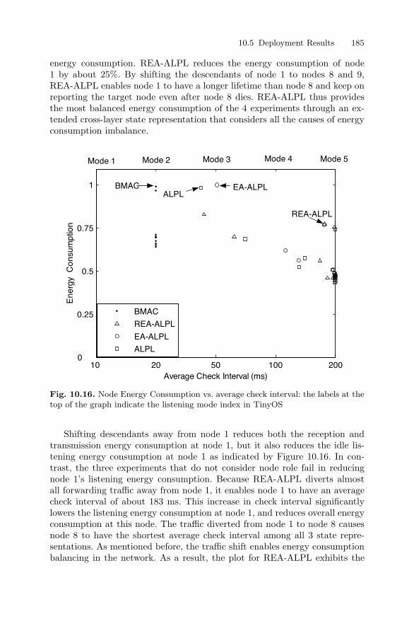
10.5 Deployment Results 185
energy consumption. REA-ALPL reduces the energy consumption of node1 by about 25%. By shifting the descendants of node 1 to nodes 8 and 9,REA-ALPL enables node 1 to have a longer lifetime than node 8 and keep onreporting the target node even after node 8 dies. REA-ALPL thus providesthe most balanced energy consumption of the 4 experiments through an ex-tended cross-layer state representation that considers all the causes of energyconsumption imbalance.
10 20 50 100 2000
0.25
0.5
0.75
1
Average Check Interval (ms)
Ene
rgy
Con
sum
ptio
n
Mode 1 Mode 2 Mode 3 Mode 4 Mode 5
REA-ALPL
ALPLEA-ALPLBMAC
BMAC
REA-ALPL
EA-ALPL
ALPL
Fig. 10.16. Node Energy Consumption vs. average check interval: the labels at thetop of the graph indicate the listening mode index in TinyOS
Shifting descendants away from node 1 reduces both the reception andtransmission energy consumption at node 1, but it also reduces the idle lis-tening energy consumption at node 1 as indicated by Figure 10.16. In con-trast, the three experiments that do not consider node role fail in reducingnode 1’s listening energy consumption. Because REA-ALPL diverts almostall forwarding traffic away from node 1, it enables node 1 to have an averagecheck interval of about 183 ms. This increase in check interval significantlylowers the listening energy consumption at node 1, and reduces overall energyconsumption at this node. The traffic diverted from node 1 to node 8 causesnode 8 to have the shortest average check interval among all 3 state repre-sentations. As mentioned before, the traffic shift enables energy consumptionbalancing in the network. As a result, the plot for REA-ALPL exhibits the
186 10 Optimization of an RF Sensor Network
lowest variation in the energy consumption of the 4 most loaded nodes for allexperiments.
Through its consideration of a more comprehensive definition of node statethat includes role information, REA-ALPL has yielded better load balancingin the event-driven tracking network experiments. In particular, it has shiftedthe traffic load away from the nodes with high sensing activity. This trafficshift has reduced the energy consumption of the busiest node in the networkby 23%, resulting in significant improvement of network lifetime and ensuringthat the nodes that detect the event remain active for as long as possible.
10.6 Discussion
This chapter has proposed a framework for greedy cross-layer local optimiza-tions in sensor networks that reduces overall energy consumption in the net-work and promotes load balancing among nodes to customize network be-havior to an application’s performance requirements. The framework enablesnodes to use their local and neighborhood state information to determinetheir behavior at the MAC layer and at the network layer. At the networklayer, a flexible cost function enables nodes to customize routing cost metricsaccording to an application’s performance requirements. At the MAC layer,the nodes set their check intervals in BMAC according to their local state.Bringing together the optimizations at the network and MAC layers, ALPLis a cross-layer mechanism that ensures seamless adaptation to local state.
We have validated the framework through two sets of experiments on atest-bed of sensor nodes. The first set of experiments represented a typicaltime-driven monitoring sensor network with a single data sink. The second setof experiments was an event-driven network that modeled a target-trackingapplication.
The experiments have explored three representations for local node state.The analysis and results show that including more information from acrossthe network stack into the local state representation better reflects nodes’energy profiles and enables more informed adaptations of network behavior.In the time-driven case, the state representation combining duty cycle anddescendants yields the most balanced energy consumption distribution. Inthe event-driven case, the state representation that includes role, duty cycle,and descendants yields the most balanced spread of energy consumption forthe event-driven case.
The adaptive and flexible nature of Jurdak’s framework supports the dy-namic nature of sensor networks and can exploit local state information aboutthe present, the past, and the predicted future state of sensor nodes to reduceenergy consumption. We have studied how adapting listening modes to thenode’s current logical topology position (which represents the node’s presentstate), duty cycle (which represents the node’s past state), and role (which
10.6 Discussion 187
represents the node’s predicted future state) can reduce the global networkenergy consumption and the local energy consumption at each node.
The use of a proactive routing strategy for sensor networks requires carefultuning of the routing update period for the network application in order tobalance route adaptivity and energy efficiency. In long term monitoring ap-plications, sending route update message with a period of the same order ofdata message periods ensures that the communication overhead of proactiverouting is small.
One concern of using greedy approaches is that local decisions may notbe globally optimal. For instance, a well-known case for greedy approaches iswhen the cheapest next hop does not represent the best path to the desti-nation. In Jurdak’s framework’s implementation, the shortest path algorithmin MintRoute uses a modified cost metric including link quality and energyto route packets to the next hop. Because each node learns its hop count tothe base station by adding a single hop to its parent hop count, nodes areguaranteed to have an accurate view of their hop count. In contrast, nodeslearn the link quality and energy cost metrics for their direct neighbors only,so nodes may not adapt instantaneously to abrupt changes for these metricselsewhere in the network. However, we have observed through our deploymentthat the nodes’ energy cost metrics change gradually rather than abruptly. Asfor link qualities, transient changes occur due to movement of objects aroundthe nodes, but the high data yield rate in our deployment has shown thatthese changes have minimal effect on data delivery or energy savings.
Jurdak’s customized framework adopts BMAC for the MAC layer pro-tocols and introduces ALPL to interface the MAC layer with a proactivestrategy at the routing layer. For any proactive routing protocol, ALPL doesnot significantly increase communication, processing, or storage complexity.The results in Section 10.5 have shown that the communication overhead of afew bits of state information in periodic routing messages is a small price topay for the energy savings of ALPL. In terms of processing complexity, costmetric calculations in ALPL involve simple arithmetic operations and rout-ing decisions involve a few simple conditional statements. Finally, the stateinformation stored at each node is a function of node density and not networksize, which adds scalability to the greedy approach.
Because of the reduced transmission power in our deployment and thelimited space in the laboratory, each node had an average of about 4 neigh-bors, yielding a relatively high network density. The high node density in ourexperiments raised the degree of contention among nodes. Coupled with theframework’s locally optimal decisions, the experiments have confirmed thatthe framework is scalable to large or dense networks despite the limited sizeof our network test-bed.
ALPL attempts to address the cross-layer design challenges discussed inSection 7.3.3. ALPL’s design advocates long-term proliferation as it providesa modular framework for new services to enable optimization different net-work parameters. The framework in this chapter adheres to the guidelines of
188 10 Optimization of an RF Sensor Network
the SP architecture [149] that designates the “thin waist” of a sensor networkarchitecture to be between the MAC and the routing layers. ALPL also pro-vides a holistic perspective of performance optimization, enabling algorithmsat different layers to influence the listening mode. Finally, ALPL clearly iden-tifies the interactions with current protocols, mainly the routing and the MACprotocols, and it outlines the required configurations for maintaining soundnetwork operation.
Reduction of global network energy consumption through local decisionsis an approach that is widely applicable to many sensor network applicationsand quality-of-service requirements. Jurdak’s framework is independent of theunderlying routing protocol or MAC protocol. Instead, it can build on otherunderlying mechanisms with a modular design to optimize the behavior ofother ad hoc and sensor network applications.
11
UWB Ad Hoc Network
This chapter customizes Jurdak’s optimization framework for UWB ad hocnetworks in order to promote 4 performance goals: (1) maximizing throughput;(2) promoting fair access; (3) minimizing connection setup latency; and (4)minimizing control overhead. Figure 11.1 shows the customized frameworkto achieve the global policy for an UWB network. Each node maintains alocal state table that includes perceived interference, received radio power,communication resource allocation for different traffic classes, and reliability.Nodes use this state information to adapt the transmission rate and powerof their active links in order to maintain link quality guarantees. Nodes alsoadapt the neighbor costs and the period of their state declaration (hello)messages according to changes in local and neighborhood state.
Within the optimization framework, we present U-MAC [200], an adaptiveMedium Access Control (MAC) protocol for UWB in which nodes periodicallydeclare their current state, so that neighbors can proactively assign power andrate values for new links locally in order to optimize global network perfor-mance. Simulations comparing U-MAC to the reactive approach confirm thatU-MAC lowers link setup latency and control overhead, doubles the through-put and adapts better to high network loads. Simulations also reveal that thebasic form of U-MAC favors nodes that are closer to the receiver. As a result,we also introduce novel mechanisms that control the radius around a receiverwithin which nodes can have fair access to it. We show through simulationsthe effect of the mechanisms on the tradeoff between network throughput andfair access.
Portions reprinted, with permission, from (R. Jurdak, P. Baldi, and C. V. Lopes.“U-MAC: A Proactive and Adaptive UWB Medium Access Control Protocol”.Wiley Wireless Communications and Mobile Computing Journal, 5(5):551-566,2005). c©2005 Wiley
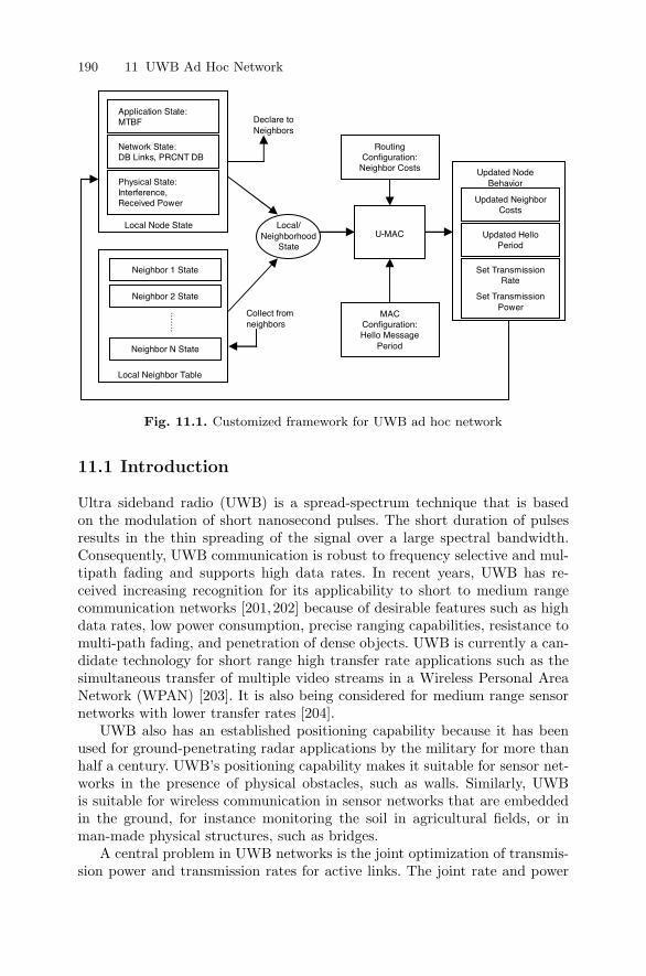
190 11 UWB Ad Hoc Network
Application State: MTBF
Network State: DB Links, PRCNT DB
Physical State: Interference, Received Power
Neighbor 1 State
Neighbor 2 State
Neighbor N State
Local Node State
.……
Local Neighbor Table
Collect from neighbors
Local/ Neighborhood
State
Declare to Neighbors
U-MAC
Routing Configuration:
Neighbor Costs
Updated Neighbor Costs
Updated Hello Period
Updated Node Behavior
MAC Configuration: Hello Message
Period
Set Transmission Rate
Set Transmission Power
Fig. 11.1. Customized framework for UWB ad hoc network
11.1 Introduction
Ultra sideband radio (UWB) is a spread-spectrum technique that is basedon the modulation of short nanosecond pulses. The short duration of pulsesresults in the thin spreading of the signal over a large spectral bandwidth.Consequently, UWB communication is robust to frequency selective and mul-tipath fading and supports high data rates. In recent years, UWB has re-ceived increasing recognition for its applicability to short to medium rangecommunication networks [201,202] because of desirable features such as highdata rates, low power consumption, precise ranging capabilities, resistance tomulti-path fading, and penetration of dense objects. UWB is currently a can-didate technology for short range high transfer rate applications such as thesimultaneous transfer of multiple video streams in a Wireless Personal AreaNetwork (WPAN) [203]. It is also being considered for medium range sensornetworks with lower transfer rates [204].
UWB also has an established positioning capability because it has beenused for ground-penetrating radar applications by the military for more thanhalf a century. UWB’s positioning capability makes it suitable for sensor net-works in the presence of physical obstacles, such as walls. Similarly, UWBis suitable for wireless communication in sensor networks that are embeddedin the ground, for instance monitoring the soil in agricultural fields, or inman-made physical structures, such as bridges.
A central problem in UWB networks is the joint optimization of transmis-sion power and transmission rates for active links. The joint rate and power
11.1 Introduction 191
assignment problem in UWB involves complex tradeoffs between fair rateassignment, network efficiency, and QoS, which cut across traditional layerboundaries. A high power link may achieve high transmission rates, but italso causes high interference which limits the rate available to neighboringlinks. On the other hand, a low power link promotes fair access to the wirelessmedium but yields lower transmission rates. Thus, nodes must collaborativelydetermine the optimal rate and power values for new links in the network.
Another important consideration for rate and power assignments in UWBnetworks is fair access among nodes at different distances from a commonreceiver, especially in ad hoc networks with dynamic topologies. An inher-ent property of wireless communications is that transmission rates drop withincreasing distance. This effect is even more pronounced in UWB commu-nications, where the strong correlation of transmission rates with multiuserinterference levels further increases the impact of relative distances on trans-mission rates. This impact may be unsuitable for applications that requireall the network nodes to have fair access to the medium regardless of dis-tance. The fair access requirement in such applications imposes an additionalconstraint on the choice of transmission power.
So far, UWB research has been primarily confined to the investigation ofthe behavior of the physical layer [10, 205]. Research at higher layers of thenetwork stack has been somewhat limited. Previous research proposals forhigher layers considered an underlying Radio Frequency (RF) physical layer,so most of these proposals are not suitable for UWB networks. For instance,the existing wireless MAC protocols [179] for RF networks do not meet theneed of UWB networks for joint rate and power assignment, hence the needfor new UWB MAC protocols. There have been recent attempts to developmechanisms for UWB networks at the MAC layer. The work in [206] proposesa simple reactive multiple access protocol that defines the handshaking proce-dure to establish a new link. The work in [207, 208] discusses a protocol thatuses periodic state updates to allow nodes to jointly assign rate and powerassignment values locally at each node.
Here, we examine the U-MAC (Ultra sideband MAC) protocol that jointlyassigns rate and power values in UWB networks, and reduces the controlmessaging and latency required for link establishment. To ensure collabo-ration among nodes, U-MAC requires nodes to periodically announce theirstate information (from the application, network, MAC, and physical layers)in hello messages, so that any node can locally select appropriate rate andpower values for a link request without polling neighbors. In U-MAC, thehello message period adapts to the stability of network state, to avoid sendingfrequent updates unnecessarily. U-MAC also provides a mechanism to adjustthe radius around a receiver within which all nodes get fair access to the re-ceiver. Furthermore, the protocol’s framework supports the future integrationof multihop links [175], which limits the impact of distance on fairness andthe internode interference.
192 11 UWB Ad Hoc Network
Within the emerging UWB MAC framework, the main contributions inthis chapter are:
• The introduction of adaptive periods for hello messages in an UWB net-work so that control message overhead is minimized
• A comparative assessment with the reactive approach regarding controloverhead, link setup latency, network throughput and adaptability
• The development of mechanisms that promote fair access among nodes inan UWB network
The remainder of the chapter is organized as follows. Section 11.2 reviewsthe fundamental concepts in UWB radio and provides the framework uponwhich we design U-MAC. Section 11.3 introduces U-MAC and explains themechanisms and features that characterize this protocol. Section 11.4 presentsthe simulation results for U-MAC. Section 11.5 discusses U-MAC in light ofexisting literature and future research directions.
11.2 UWB Network Principles
11.2.1 UWB Principles
Recently, UWB radio has received increasing recognition for its applicabilityto multiuser wireless communication networks. UWB radio relies on periodicsequences of short subnanosecond pulses (referred to as monocycles) for datatransmission. The short duration of UWB pulses yields a low power spectrallywide signal. In a single sender/receiver environment, a common modulationtechnique used with UWB radio is Pulse Position Modulation (PPM), whichencodes symbols by shifting the monocycles according to the following expres-sion:
s(t) =∞∑
i=−∞
NS−1∑j=0
g(t − jTf − biτ) (11.1)
where s(t) is the transmitted signal, g(t) is the pulse, and Tf is the frame time.Ns is the number of pulses that encode each symbol, and the sequence bi en-codes the information bits. Win and Scholtz [205] have proposed a multiuseraccess scheme for UWB using time-hopping (TH) codes. TH-codes accom-modate multiple users by further shifting the pulse g(t) according to one ofmany chipping codes. Consequently, UWB radio has potential for supportingmultiple users within the same frequency and spatial channel.
In a centralized UWB network, the base station could send periodic bea-cons to allow nodes to stay synchronized. Global synchronization among nodesin an ad hoc UWB network requires excessive signalling overhead, which isa waste of valuable battery resources in mobile nodes. Consequently, it ismore realistic to assume that only each sender and receiver that share a link
11.2 UWB Network Principles 193
are synchronized. This assumption may lead to collisions of some monocyclesamong different links.
The impact of monocycle collisions due to the lack of global synchroniza-tion is reduced by sending multiple pulses for each symbol at the source as aform of forward error correction, so that collisions contribute only to mutualinterference. Provided that proper quality margins are set, collisions only re-duce signal quality and do not affect correct reception of data at the receiver1.
The binary bit rate of an M -ary PPM UWB signal is given by the followingexpression [209]:
Rb =1
TfNSlog2M (11.2)
Both Tf and M are difficult to modify in an UWB system. Changing M fordifferent transmissions is undesirable for communication systems since it leadsto processing overhead. Similarly, modifying Tf for each transmission increasesthe complexity of the hardware design of the system. Thus, the simplest wayto adjust Rb is to vary the value of NS . The only requirement for allowingdifferent NS values is that the receiver of each link must integrate the correctnumber of pulses for each symbol received on that link. A protocol that isadaptive to network behavior should vary NS based on interference levels inthe network. More specifically, high interference levels increase the probabilityof pulse collisions, which requires more pulses per symbol.
We adopt the framework of Cuomo et al. [206] for an UWB radio re-source sharing model that assumes continuous values for Rb. The frameworkconsiders that a new link request arrives when there are N pairs of communi-cating UWB terminals, with each pair consisting of one transmitter and onereceiver. Each pair of sender and receiver are synchronized to the TH-code oftheir common link, and both background and UWB noise impact the SNR ofUWB links. Consequently, the SNR at the receiver of the ith link is:
SNRi =Pi
RiPLii(ηi + Tfσ2∑N
k=1,k �=i Pkgki)(11.3)
where Pi is the power of the ith transmitter, Ri is the binary bit rate of theith link, ηi is the background noise energy plus interference from non-UWBsources at receiver i, PLij is the path loss from the ith transmitter to thejth receiver, gki is the path gain from the kth transmitter to the ith receiver,and σ2 is a parameter depending on the shape of the monocycle. Commonvalues for the above parameters are [205]: Tf = 100ns; σ2 = 1.9966 × 10⁻³;and η = 2.568 × 10⁻²¹V 2s; with a pulse duration of 0.75ns.
11.2.2 UWB Traffic Classes
We consider two traffic classes for UWB networks, in accordance with thespecifications of the European Whyless Project [206,210,211], to address the1 This concept is similar to increasing the processing gain in CDMA systems.

194 11 UWB Ad Hoc Network
requirements of different application types: (1) Reserved Bandwidth (RB);and (2) Dynamic Bandwidth (DB).
The RB traffic class is geared towards continuous, real-time or multimediatraffic, since it requires quality guarantees prior to establishing a link. Thecontinuous nature of traffic that exploits the RB traffic class requires that thelink rate remain constant throughout the lifetime of the link.
DB traffic does not offer any rate guarantees and is thus suitable for best-effort data, such as internet traffic. As the name implies, the rate of a linkis dynamic and elastic, and depends on the number of other active DB linksand on interference levels in the network. For instance, if the traffic load in anetwork is low, then individual DB links may use higher rates.
In short, the goal of RB traffic is to offer a certain quality-of-service for thesender under varying network conditions. The goal of DB traffic is to provideadaptive and efficient overall network behavior for asynchronous data, and toensure a constant interference level of bursty traffic by modifying rates of allDB channels dynamically.
11.3 U-MAC Protocol
This section presents the design details of the U-MAC protocol. Section 11.3.1defines the joint power and rate assignment problem in UWB networks. Sec-tion 11.3.2 provides an overview of the U-MAC protocol. Section 11.3.3 dis-cusses the topology consideration in U-MAC. Section 11.3.4 covers the peri-odic internode interactions in U-MAC, namely the periodic hello messages.Section 11.3.5 proceeds to explore the interlayer interactions within a nodefor determining the transmission rate and power for a new link locally, beforeproceeding with a link establishment request. Finally, Section 11.3.6 focuseson the tunable MSI margin in U-MAC, which controls communication radiiand fairness.
11.3.1 Problem Definition
U-MAC addresses the joint rate and power assignment problem for UWBlinks for both RB and DB traffic. In general, each node in the network is thereceiver for a certain number of communication links. Based on the qualityrequirements of its currently active links, the node can tolerate a finite amountof additional interference, referred to as maximum sustainable interference(MSI) [212]. The MSI at each node must be efficiently and fairly divided upbetween RB and DB traffic and among links of each traffic class.
Initially, each node’s resources are split evenly between RB and DB traffic.As a node starts receiving link requests, the MSI portion allocated to eachtraffic type can adapt to the relative number of links in each traffic class. Ingeneral, at any point in time, each node allocates a portion λ of its MSI to DBtraffic, and the remaining portion (1 − λ) to RB traffic, where λ is less than
11.3 U-MAC Protocol 195
one. Section 11.3.6 provides a more detailed discussion of an MSI allocationtechnique that avoids starvation.
From the transmitting node’s perspective, the challenge is selecting ratesand power levels for new links that adhere to the MSI states of it’s neighbors.The generic relation between link quality, transmission rate, and transmissionpower is:
Quality α (Power
Rate × Noise) (11.4)
During the lifetime of the link, new communication links may cause the noiseto increase, which subsequently causes quality degradation of the link. Avoid-ing quality degradation can be achieved in several ways:
1. Increasing transmission power2. Decreasing transmission rate3. Providing a quality margin above the minimum quality requirement ini-
tially so that when new links are set up, the link can tolerate additionalinterference
Although increasing the transmission power maintains link quality and trans-mission rate, it degrades the quality of neighboring links which may requireadditional power or rate adjustments in the network. Furthermore, the FCChas imposed tight limits on UWB emissions [213], so increasing transmissionpower to maintain quality is impractical. Alternatively, the link transmissionrates can be lowered to maintain quality in response to increasing interfer-ence. This option does not require reconfiguration of neighboring links, but itleads to inefficient use of the medium and may cause quality violations if thelink carries RB traffic. Thus, U-MAC allows reducing link transmission ratesonly for DB traffic. Finally, providing quality margins avoids both rate andpower adjustments of any active links, which suits RB links. The drawback ofquality margins is that they also lead to less than optimal medium utilization.
U-MAC adopts Signal to Noise Ratio (SNR) as the main link signal qualitymetric. The SNR of a new link must have some margin above the minimumacceptable SNR for the link. In U-MAC, the parameter µ determines the sizeof the SNR quality margin of links (see (11.7) and (11.9) below). The value ofµ could be static or adaptive to the spatial distribution of nodes, the trafficload, and the lifetime of the link. The rest of the discussion assumes thatsource nodes set the SNR margin µ statically for simplicity.
11.3.2 Protocol Overview
The U-MAC discussion in this chapter covers both RB and DB traffic fora single hop distributed topology. The discussion for a distributed topologycould easily apply to the centralized or hybrid topology, since the distributedcase is inherently more complex in nature. Furthermore, a single hop topologycould be extended to a multihop topology through the use of a global costfunction to enable multihop links [175].
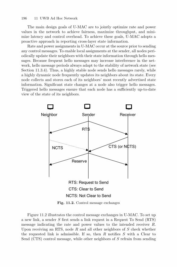
196 11 UWB Ad Hoc Network
The main design goals of U-MAC are to jointly optimize rate and powervalues in the network to achieve fairness, maximize throughput, and mini-mize latency and control overhead. To achieve these goals, U-MAC adopts aproactive approach in reporting cross-layer state information.
Rate and power assignments in U-MAC occur at the source prior to sendingany control messages. To enable local assignments at the sender, all nodes peri-odically update their neighbors with their state information through hello mes-sages. Because frequent hello messages may increase interference in the net-work, hello message periods always adapt to the stability of network state (seeSection 11.3.4). Thus, a highly stable node sends hello messages rarely, whilea highly dynamic node frequently updates its neighbors about its state. Everynode collects and stores each of its neighbors’ most recently advertised stateinformation. Significant state changes at a node also trigger hello messages.Triggered hello messages ensure that each node has a sufficiently up-to-dateview of the state of its neighbors.
Sender
RTS
CTS (or NCTS)
Receiver
NCTS
Reserve
RTS: Request to Send
CTS: Clear to Send
NCTS: Not Clear to Send
Neighbor
Fig. 11.2. Control message exchanges
Figure 11.2 illustrates the control message exchanges in U-MAC. To set upa new link, a sender S first sends a link request in a Request To Send (RTS)message indicating the rate and power values to the intended receiver R.Upon receiving an RTS, node R and all other neighbors of S check whetherthe requested link is admissible. If so, then R notifies S with a Clear toSend (CTS) control message, while other neighbors of S refrain from sending
11.3 U-MAC Protocol 197
any replies if the link parameters are satisfactory. However, if the receiver nodeR or any other neighbor of S does not agree with the parameters of the newlink, then that neighbor notifies S with a Not Clear to Send Message (NCTS)that it should reduce either the transmit power or rate or both. After S collectsall the replies, it declares the duration and parameters of the new link (whichmay have changed according to neighbor replies) in a Reserve message, andimmediately sets up the link.
11.3.3 Topology
U-MAC supports a hybrid multihop topology, which provides a node with flex-ibility in switching between centralized mode when an access point is available,or ad hoc mode when an access point is not reachable. To determine its cur-rent mode of operation, a node monitors a dedicated hello message channel.Whenever it detects any access point hello messages, it switches to centralizedmode. The node must hear access point hello messages periodically; otherwise,it switches to distributed mode. The remainder of the discussion in this sectionfocuses on the case of distributed mode in a single hop topology. U-MAC caneasily be extended to support multihop links through a global cost functionthat quantifies link costs in order to determine optimal routes [175].
11.3.4 Hello Messages
U-MAC requires nodes to advertise their local states periodically throughhello messages [214], which provides for quick and appropriate rate and powerassignments in the network. Note that although hello messages are periodic forone node, they are asynchronous among different nodes in the network, whichhelps avoid hello message interference from different nodes. Many factors con-tribute to avoiding several simultaneous transmissions of hello messages:
• Because the hello message period in each node depends on the node’sstability, hello periods are not the same across nodes
• Clock skews contribute favorably to collision avoidance in hello messages ofnodes that have the same hello message period and that enter the networkat the same time
• The transmission time of hello messages is much shorter than typical hellomessage periods which further reduces the chances of collisions
Hello messages implicitly provide nodes with ranging information about neigh-bors, and they explicitly advertise important local parameters to neighboringnodes. Storing recent neighbor state information locally enables a node tomake decisions on rate and power assignments for new links, and to makerouting decisions for multihop links.
First, nodes use hello messages to determine distances of neighboringnodes. Each node sends its hello message at a fixed power level know a priorito all nodes. Whenever a node receives a hello message from a neighbor, it
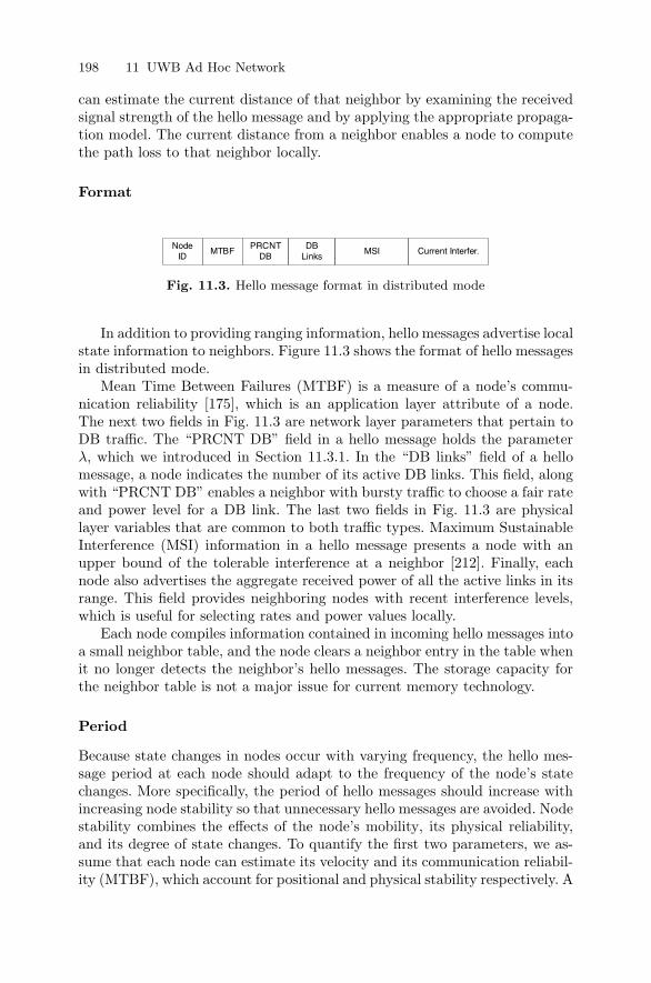
198 11 UWB Ad Hoc Network
can estimate the current distance of that neighbor by examining the receivedsignal strength of the hello message and by applying the appropriate propaga-tion model. The current distance from a neighbor enables a node to computethe path loss to that neighbor locally.
Format
NodeID
MTBFPRCNT
DBDB
LinksMSI Current Interfer.
Fig. 11.3. Hello message format in distributed mode
In addition to providing ranging information, hello messages advertise localstate information to neighbors. Figure 11.3 shows the format of hello messagesin distributed mode.
Mean Time Between Failures (MTBF) is a measure of a node’s commu-nication reliability [175], which is an application layer attribute of a node.The next two fields in Fig. 11.3 are network layer parameters that pertain toDB traffic. The “PRCNT DB” field in a hello message holds the parameterλ, which we introduced in Section 11.3.1. In the “DB links” field of a hellomessage, a node indicates the number of its active DB links. This field, alongwith “PRCNT DB” enables a neighbor with bursty traffic to choose a fair rateand power level for a DB link. The last two fields in Fig. 11.3 are physicallayer variables that are common to both traffic types. Maximum SustainableInterference (MSI) information in a hello message presents a node with anupper bound of the tolerable interference at a neighbor [212]. Finally, eachnode also advertises the aggregate received power of all the active links in itsrange. This field provides neighboring nodes with recent interference levels,which is useful for selecting rates and power values locally.
Each node compiles information contained in incoming hello messages intoa small neighbor table, and the node clears a neighbor entry in the table whenit no longer detects the neighbor’s hello messages. The storage capacity forthe neighbor table is not a major issue for current memory technology.
Period
Because state changes in nodes occur with varying frequency, the hello mes-sage period at each node should adapt to the frequency of the node’s statechanges. More specifically, the period of hello messages should increase withincreasing node stability so that unnecessary hello messages are avoided. Nodestability combines the effects of the node’s mobility, its physical reliability,and its degree of state changes. To quantify the first two parameters, we as-sume that each node can estimate its velocity and its communication reliabil-ity (MTBF), which account for positional and physical stability respectively. A

11.3 U-MAC Protocol 199
node is physically reliable if its hardware and software components are robustand do not experience frequent interruptions in service. A node has positionaland communication reliability if its velocity relative to its neighbors is small.Baldi et al. [175] provide a combined measure of these two factors: C(quality).
To monitor the stability of its interference state, each node can compareits current state to the state it advertised in its last hello message. Significantchanges in MSI or current interference levels trigger the node to send an earlyhello message and lower its hello message period. The creation of a new linkcould result in state changes at more than one node and trigger them to issuehello messages. Consequently, nodes that detect local state changes upon thecreation of a new link must wait a random time (within a maximum waittime) before sending a hello message in order to minimize interference on thehello message TH-code.
We define a new Boolean cost metric C(state) which takes the value of oneif either MSI or the current interference at a node vary beyond their respectivethresholds, and takes the value of zero otherwise. When C(state) has a valueof one, a hello message is triggered. We also define a compound cost metric:
C(stability) = C(quality) + C(state) (11.5)
which represents the overall stability of a node. U-MAC varies the hello mes-sage period at each node linearly with C(stability) at that node, as indicatedbelow:
Thello =
⎧⎨⎩
Tmin C(stability) ≥ Cmax
K + Tmax Cmin < C(stability) < Cmax
Tmax C(stability) ≤ Cmin
K = Tmin−Tmax
Cmax−Cmin× C(stability)
where Tmax and Tmin are the maximum and minimum time between hellomessages respectively, and Cmax and Cmin represent the upper and lowerbounds of C(stability) respectively. Finally, nodes that do not experience statechanges between two consecutive hello messages increase their hello messageperiod by 1 second as long as the period is lower than Tmax.
11.3.5 Rate and Power Assignment
In a centralized UWB network, the access point determines optimal rate andpower assignments. Nodes that are out of range of an access point and nodesin UWB ad hoc networks must assign channel rates and transmit power levelsin a distributed way. Choosing an appropriate channel rate and power is notsimple, since nodes do not have a global view of network state. Each node canuse its neighbor state information to select appropriate parameters for a newlink request.
200 11 UWB Ad Hoc Network
Most conventional wireless networks that use multiple channels require anexplicit channel separation mechanism, such as TDMA or FDMA, to accom-modate multiple users [179]. In UWB networks, each pseudo-random time-hopping (TH) code constitutes a separate channel.
In U-MAC, all nodes use a known TH-code as a common control chan-nel. We also assign another fixed TH-code to a dedicated channel for hellomessages. Occasional hello message losses are not as critical as control mes-sage losses. We assume that nodes synchronize prior to sending and receivinghello messages and control messages. To achieve on-demand synchronizationon these two channels, one node could send a short beacon prior to sendingits control or hello message to allow neighbors to synchronize to its transmis-sion, which is similar to IEEE 802.11 [5] synchronization for the distributedcase. Finally, each of the remaining TH-codes is a potential one-way separatedata channel. Synchronization on data channels is only required between eachsender and receiver pair of an active link.
RB traffic
The RB traffic class accommodates data streams that require a particularquality-of-service. The two quality parameters of interest are the link trans-mission rate and the SNR at the receiver of the link. Providing a link rateguarantee often prevents any adjustment of the transmit power level while thelink is active, in order to maintain the signal integrity at the receiver. Thus,the goal is locally assigning link rate and power values that make efficientuse of the medium, achieve fairness among nodes, and ensure that the qualityguarantees (transmission rate and minimum SNR) can be maintained for thelifetime of the link.
First, a node S determines the maximum allowable transmit power levelfor all neighbors, using the following equation [206]:
Pallowed = min{ (1 − λi)MSIi × PLsi
Tfσ2} (11.6)
where MSIi is the MSI value announced by the ith node, and PLsi is thepath loss from node S to neighbor i. In short, node S must select a powerlevel that does not violate the interference threshold of any active links at itsneighbors. If there are no active links in the network, then Pallowed takes thevalue of Pmax.
Next, node S must select an appropriate rate for the new link to thereceiver R, through the expression:
RS =min(Pallowed, Pmax)/PLsr
SNRmin × µ(ηr + Ur)(11.7)
where Pmax is the maximum allowable emitted power from an UWB trans-mitter, Ur is the combined received power level at the intended receiver, andηr is the thermal noise level.
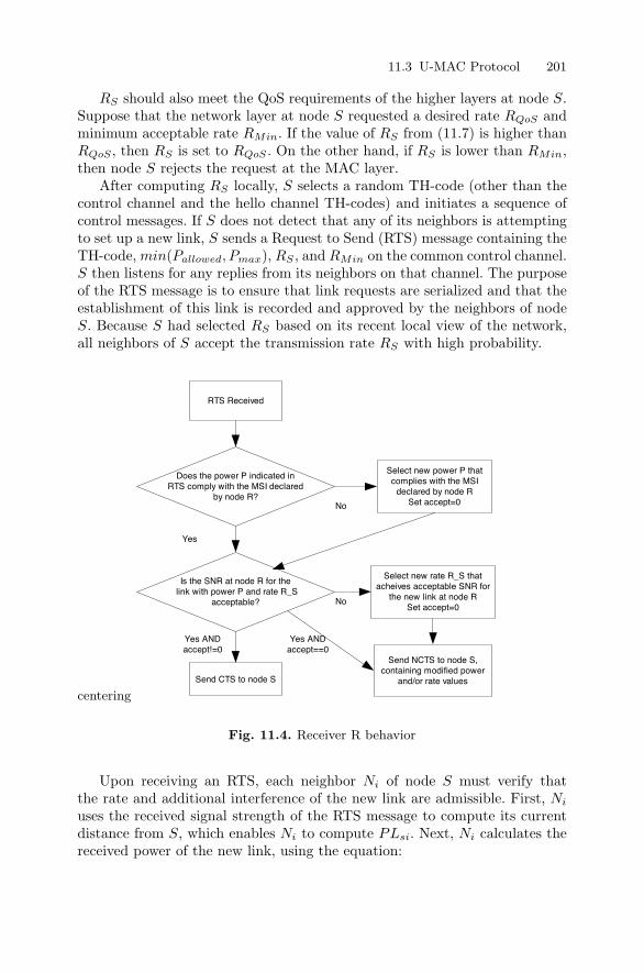
11.3 U-MAC Protocol 201
RS should also meet the QoS requirements of the higher layers at node S.Suppose that the network layer at node S requested a desired rate RQoS andminimum acceptable rate RMin. If the value of RS from (11.7) is higher thanRQoS , then RS is set to RQoS . On the other hand, if RS is lower than RMin,then node S rejects the request at the MAC layer.
After computing RS locally, S selects a random TH-code (other than thecontrol channel and the hello channel TH-codes) and initiates a sequence ofcontrol messages. If S does not detect that any of its neighbors is attemptingto set up a new link, S sends a Request to Send (RTS) message containing theTH-code, min(Pallowed, Pmax), RS , and RMin on the common control channel.S then listens for any replies from its neighbors on that channel. The purposeof the RTS message is to ensure that link requests are serialized and that theestablishment of this link is recorded and approved by the neighbors of nodeS. Because S had selected RS based on its recent local view of the network,all neighbors of S accept the transmission rate RS with high probability.
centering
Yes ANDaccept==0
Yes ANDaccept!=0
No
No
Does the power P indicated inRTS comply with the MSI declared
by node R?
RTS Received
Is the SNR at node R for the link with power P and rate R_S
acceptable?
Select new power P thatcomplies with the MSI
declared by node RSet accept=0
Send CTS to node S
Select new rate R_S thatacheives acceptable SNR for
the new link at node RSet accept=0
Yes
Send NCTS to node S,containing modified power
and/or rate values
Fig. 11.4. Receiver R behavior
Upon receiving an RTS, each neighbor Ni of node S must verify thatthe rate and additional interference of the new link are admissible. First, Ni
uses the received signal strength of the RTS message to compute its currentdistance from S, which enables Ni to compute PLsi. Next, Ni calculates thereceived power of the new link, using the equation:
202 11 UWB Ad Hoc Network
PRi =min(Pallowed, Pmax)
PLsi(11.8)
The intended receiver R must check for two additional conditions in orderbefore admitting the new link: (1) the received power of the new link doesnot exceed the MSI that R advertised in it most recent hello message; and (2)the new link has an acceptable signal to noise ratio at R. If the link requestsatisfies both (1) and (2), then R sends a Clear To Send (CTS) message tonode S immediately, otherwise R must select the appropriate rate and/orpower and include them in a Not Clear to Send (NCTS) message to S.
If the link request exceeds the declared MSI of node R, then R computesthe allowable received power PRallowed from neighbor S. Subsequently, nodeR can then compute the rate at which a signal from S arriving at R withpower PRallowed would have an acceptable signal quality:
Rr =PRallowed
SNRMin × µ(ηr + Ur)(11.9)
The other case is that the link request does not violate node R’s MSI butfails to achieve an acceptable SNR at node R. In that case, node R usesPallowed/PLsi instead of PRallowed in (11.9) to get the Rr that would result inan acceptable SNR for the new link at node R. In addition, node R could checkif the TH chosen by S closely correlates with one of the TH-codes currentlyused by other links in its neighborhood [205].
Node S waits for incoming neighbors’ replies. If S receives only a CTSmessage, then it sends a “Reserve” message indicating the rate, power andduration of its link reservation, and it immediately sets up a link to node R.The “Reserve” message also allows the receiver to synchronize to the sender’sTH code. If at least one NCTS arrives at S, then S adjusts Pallowed and RS
in order to satisfy the updated interference state of its neighbors. If the newvalue of RS is higher than RMin, then S sends a “Reserve” message and setsup the link with the newly chosen rate and power. Otherwise, the link requestfails.
Upon reception of the “Reserve” message and establishment of the link,all neighbors of S update their MSI and current interference levels. If anyneighbor Ni detects an appreciable variation in either of the two parametersas a result of the update, Ni issues a hello message to inform its neighborsof the state change. If any node’s hello message timer expires during a linksetup phase, the node postpones sending the hello message until after the linkrequest, to avoid inconsistent views of network state during the link request.
DB traffic
The purpose of DB traffic in UWB is to support best-effort delivery of datawithout any quality requirements. More specifically, a DB link can sacrifice
11.3 U-MAC Protocol 203
performance in order to keep interference levels constant at neighbors. In U-MAC, nodes accommodate a new DB request by lowering rates of their otheractive DB links so that the creation of the new link keeps the interference levelsconstant. Naturally, ensuring that the link rates are adaptive to network staterequires the symmetric mechanism of increasing rates once a DB transmissionends. To promote fairness, the receiver can also split its DB bandwidth equallyamong all active DB links.
A node could monitor the traffic nature of its neighborhood through hellomessages and allocate a portion of its spectrum to each traffic class. As men-tioned earlier, each node allocates λ of its MSI to DB traffic, and (1 − λ) toRB traffic. Each node further divides its DB portion equally among all activeDB links, and it adjusts all DB power levels and potentially the correspondingrates whenever a new DB link is established. If a node Ni has k active DBlinks, a new DB link would cause it to adjust the received power level of eachlink based on the expression:
PRi =MSIi × λi
k + 1(11.10)
Since nodes in the network use random TH-codes, the aggregation of severaltransmissions appear as background noise at any receiver. The addition ofanother DB link with a new TH code does not add to the interference at areceiver if the overall DB received power stays the same.
When S has DB data to send to node R, it checks the information compiledfrom recent hello messages2. For each neighbor Ni, S uses a modified versionof (11.6):
Pallowed = min{MSIi × PLsi × λi
Tfσ2(k + 1)} (11.11)
S then proceeds as in the RB case to assign a corresponding rate with anappropriate margin, to send an RTS message, and to await neighbor replies.The intended receiver R replies with CTS if it consents to the DB request, orwith NCTS if the request is not appropriate. Other neighbors of S only replyin case they do not agree with the DB request.
Once S processes all the replies, it sends a “Reserve” message and beginssending DB data. The neighbors of S that are sources to DB links hear the“Reserve” message and lower their DB link power and rates as needed toaccommodate the new DB link from S. However, two-hop neighbors of S donot detect the “Reserve” message. Suppose Nj is a two-hop neighbor of S, andNj has an active DB link with a neighbor Ni of S. When Ni detects that Nj
has not reduced its power in response to the “Reserve” message, Ni signals Nj
to lower the power (and potentially the rate) of its active DB transmissions.
2 Since λ changes rarely, the MSI triggering of hello messages ensures that neigh-boring can make DB rate selections based on a sufficiently up-to-date local viewof the network. To account for DB link changes at neighbors since the last hellomessage, S could use a margin which is dependent upon the traffic pattern.
204 11 UWB Ad Hoc Network
Modifying the power of all received DB transmissions upon the creation ofa new DB stream ensures that the aggregate received power from DB trafficremains constant at each node. Based on the size of DB traffic indicated in RTSand the granted rate in “Reserve”, each two-hop neighbor can set a timer toindicate the approximate time that this DB link will be active. When the timerfor a DB link expires, each neighbor releases the link resources, recomputesthe updated state parameters locally, and includes these changes in the nextscheduled hello message. There is no need to trigger hello messages upon aDB link expiration, since all nodes in the area set the same timer for this link,and each of them releases its resources locally. Clock skews among the nodesonly lead to instantaneous differences in local node states and do not affectthe protocol behavior.
11.3.6 MSI Margin
So far, the discussion has focused on rate and power assignment from thepoint of view of a sender. Each sender must know the interference state of itsneighbors when it sets up a new link. The interference state information thata node advertises in its hello messages is therefore the basis for transmissionpower and rate assignment at the sender. First, if Ni advertises MSINi
of itsweakest active link, one neighbor Nj may set up a link with Ni that causesMSINi
to drop to zero, which would block other nodes in the vicinity fromsetting up new links. Thus, the first challenge is to declare an MSI value thatmakes efficient use of the medium and ensures fairness. The other challengefor MSI reporting is that, as we mentioned earlier, minor changes in MSI orinterference at the node do not trigger hello messages, so nodes may haveslightly inaccurate state information about their neighbors.
To address these challenges, each node can declare a fraction of its MSI, inorder to avoid starvation of some nodes and to account for unreported minorchanges. The portion of MSI that a node declares should depend on how busya receiver it is. For example, if the average number of active links at Ni inthe recent past is low, then Ni can declare a larger portion of its MSI, since itdoes not expect to receive many more requests. On the other hand, if Ni hasmany active links on average, then it advertises a smaller MSI. We use thefollowing expression to compute the declared MSI for hello messages at nodeNi:
MSI =MSItotal × δ
active(11.12)
where MSItotal is the full MSI of the weakest link at Ni, active is the numberof active links at Ni, and δ is a topology dependent adjustable margin thattrades off fairness for throughput. In Section 11.4, we explore the effect ofvarying the values of δ on fairness and throughput.
The margin δ enforces power control, which can contribute to fairnessamong near and far nodes. Consider the case of Fig. 11.5, where both nodesA and C wish to send data to node B. We expect Pallowed at C to be higher
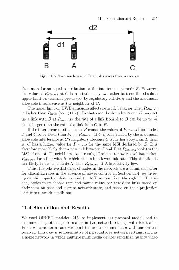
11.4 Simulation and Results 205
Fig. 11.5. Two senders at different distances from a receiver
than at A for an equal contribution to the interference at node B. However,the value of Pallowed at C is constrained by two other factors: the absoluteupper limit on transmit power (set by regulatory entities); and the maximumallowable interference at the neighbors of C.
The upper limit on UWB emissions affects network behavior when Pallowed
is higher than Pmax (see (11.7)). In that case, both nodes A and C may setup a link with B at Pmax, so the rate of a link from A to B can be up to d2
2d21
times larger than the rate of a link from C to B.If the interference state at node B causes the values of Pallowed from nodes
A and C to be lower than Pmax, Pallowed at C is constrained by the maximumallowable interference at C’s neighbors. Because C is further away from B thanA, C has a higher value for Pallowed for the same MSI declared by B. It istherefore more likely that a new link between C and B at Pallowed violates theMSI of one of C’s neighbors. As a result, C selects a power level lower thanPallowed for a link with B, which results in a lower link rate. This situation isless likely to occur at node A since Pallowed at A is relatively low.
Thus, the relative distances of nodes in the network are a dominant factorfor allocating rates in the absence of power control. In Section 11.4, we inves-tigate the impact of distance and the MSI margin δ on throughput. To thisend, nodes must choose rate and power values for new data links based ontheir view on past and current network state, and based on their projectionof future network conditions.
11.4 Simulation and Results
We used OPNET modeler [215] to implement our protocol model, and toexamine the protocol performance in two network settings with RB traffic.First, we consider a case where all the nodes communicate with one centralreceiver. This case is representative of personal area network settings, such asa home network in which multiple multimedia devices send high quality video
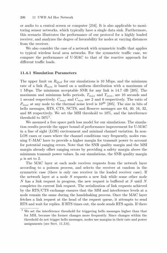
206 11 UWB Ad Hoc Network
or audio to a central screen or computer [216]. It is also applicable to moni-toring sensor networks, which typically have a single data sink. Furthermore,this scenario illustrates the performance of our protocol for a highly loadedreceiver, and analyzes the degree of favorability for nodes at varying distancesfrom the receiver.
We also consider the case of a network with symmetric traffic that appliesto typical wireless local area networks. For the symmetric traffic case, wecompare the performance of U-MAC to that of the reactive approach fordifferent traffic loads.
11.4.1 Simulation Parameters
The upper limit on RQoS for our simulations is 10 Mbps, and the minimumrate of a link Rmin is based on a uniform distribution with a maximum of1 Mbps. The minimum acceptable SNR for any link is 14.7 dB [205]. Themaximum and minimum hello periods, Tmax and Tmin, are 10 seconds and1 second respectively. Cmax and Cmin are 2 and 0 respectively. The ratio ofPmax at any node to the thermal noise level is 1020 [205]. The size in bits ofhello messages, RTS, CTS, NCTS, and Reserve messages are 64, 40, 16, 32,and 88 respectively. We set the MSI threshold to 10%, and the interferencethreshold to 50%3.
We assumed a free space path loss model for our simulations. The simula-tion results provide the upper bound of performance improvement for U-MACin a line of sight (LOS) environment and minimal channel variation. In non-LOS cases or cases where the channel conditions vary frequently, nodes run-ning U-MAC have to provide a higher margin for transmit power to accountfor potential ranging errors. Note that the SNR quality margin and the MSImargin already offset ranging errors by providing a safety margin above theminimum transmit power values. In our simulations, the SNR quality marginµ is set to 2.
The MAC layer at each node receives requests from the network layeraccording to a poisson process, and selects the receiver at random in thesymmetric case (there is only one receiver in the loaded receiver case). Ifthe network layer at a node S requests a new link while some other nodeN has a link request in progress, the new request is buffered at S until Ncompletes its current link request. The serialization of link requests achievedby the RTS/CTS exchange ensures that the MSI and interference levels at anode remain the same during the handshaking process. Once the MAC layerfetches a link request at the head of the request queue, it attempts to sendRTS and wait for replies. If RTS times out, the node sends RTS again. If there3 We set the interference threshold for triggering hello messages higher than that
for MSI, because the former changes more frequently. Since changes within thethreshold do not trigger hello messages, nodes use margins in their rate and powerassignments (see Sect. 11.3.6).
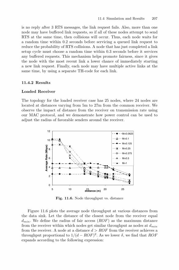
11.4 Simulation and Results 207
is no reply after 3 RTS messages, the link request fails. Also, more than onenode may have buffered link requests, so if all of these nodes attempt to sendRTS at the same time, then collisions will occur. Thus, each node waits fora random time within 0.2 seconds before servicing a queued link request toreduce the probability of RTS collisions. A node that has just completed a linksetup cycle must choose a random time within 0.3 seconds before it servicesany buffered requests. This mechanism helps promote fairness, since it givesthe node with the most recent link a lower chance of immediately startinga new link request. Finally, each node may have multiple active links at thesame time, by using a separate TH-code for each link.
11.4.2 Results
Loaded Receiver
The topology for the loaded receiver case has 25 nodes, where 24 nodes arelocated at distances varying from 5m to 27m from the common receiver. Weobserve the impact of distance from the receiver on transmission rate usingour MAC protocol, and we demonstrate how power control can be used toadjust the radius of favorable senders around the receiver.
0
2
4
6
8
10
12
5 10 15 20 25distance (m)
Ave
rag
e R
ate
(Mb
ps)
M=0.0625
M=0.1
M=0.125
M=0.25
M=0.375
M=0.5
M=1
Fig. 11.6. Node throughput vs. distance
Figure 11.6 plots the average node throughput at various distances fromthe data sink. Let the distance of the closest node from the receiver equaldmin. We define the radius of fair access (ROF ) as the maximum distancefrom the receiver within which nodes get similar throughput as nodes at dmin
from the receiver. A node at a distance d > ROF from the receiver achieves athroughput proportional to 1/(d − ROF )2. As we lower δ, we find that ROFexpands according to the following expression:
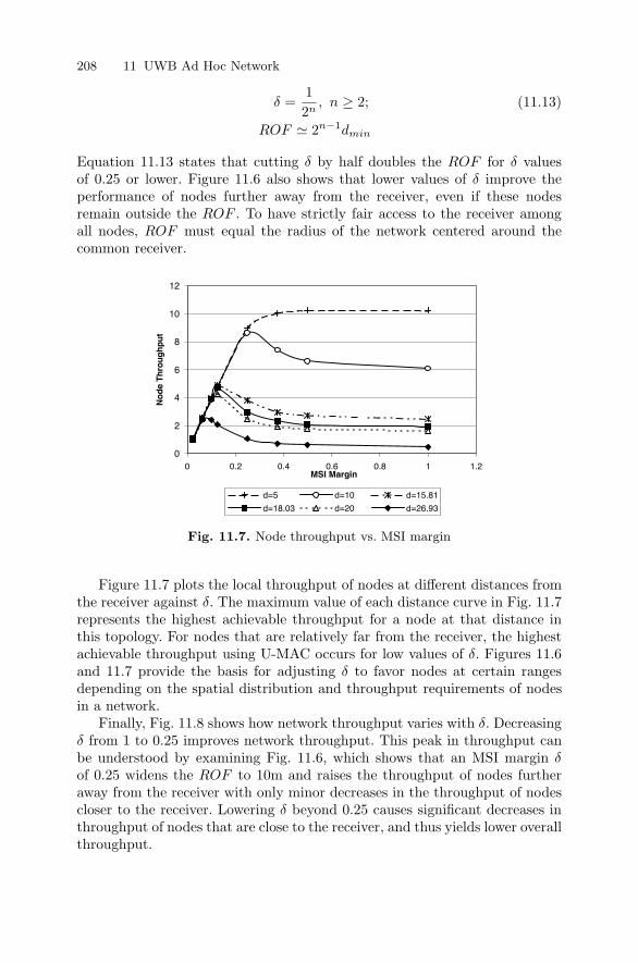
208 11 UWB Ad Hoc Network
δ =12n
, n ≥ 2; (11.13)
ROF � 2n−1dmin
Equation 11.13 states that cutting δ by half doubles the ROF for δ valuesof 0.25 or lower. Figure 11.6 also shows that lower values of δ improve theperformance of nodes further away from the receiver, even if these nodesremain outside the ROF . To have strictly fair access to the receiver amongall nodes, ROF must equal the radius of the network centered around thecommon receiver.
0
2
4
6
8
10
12
0 0.2 0.4 0.6 0.8 1 1.2MSI Margin
No
de
Th
rou
gh
pu
t
d=5 d=10 d=15.81
d=18.03 d=20 d=26.93
Fig. 11.7. Node throughput vs. MSI margin
Figure 11.7 plots the local throughput of nodes at different distances fromthe receiver against δ. The maximum value of each distance curve in Fig. 11.7represents the highest achievable throughput for a node at that distance inthis topology. For nodes that are relatively far from the receiver, the highestachievable throughput using U-MAC occurs for low values of δ. Figures 11.6and 11.7 provide the basis for adjusting δ to favor nodes at certain rangesdepending on the spatial distribution and throughput requirements of nodesin a network.
Finally, Fig. 11.8 shows how network throughput varies with δ. Decreasingδ from 1 to 0.25 improves network throughput. This peak in throughput canbe understood by examining Fig. 11.6, which shows that an MSI margin δof 0.25 widens the ROF to 10m and raises the throughput of nodes furtheraway from the receiver with only minor decreases in the throughput of nodescloser to the receiver. Lowering δ beyond 0.25 causes significant decreases inthroughput of nodes that are close to the receiver, and thus yields lower overallthroughput.
11.4 Simulation and Results 209
0
20
40
60
80
100
120
140
0 0.2 0.4 0.6 0.8 1MSI Margin
Th
rou
gh
pu
t(M
bp
s)
Fig. 11.8. Throughput vs. MSI margin
Symmetric Traffic
We considered three different topologies with 25 nodes each to investigate thesymmetric traffic case. The first topology is a grid topology with a constantnode separation distance of 5m. The second topology is a random distributionof nodes in a 100m x 100m area, with an average and minimum internode dis-tance of 10m and 5m respectively. The third topology is a random distributionof nodes in a 50m x 50m area, where the average and minimum internode dis-tances are 5m and 1m respectively. The results presented here are the averageof three topologies.
We vary the arrival rate of new link requests to observe the behavior ofthe protocol for different traffic loads. The δ value used for this scenario is 1.
We first consider the link setup latency benefits of using U-MAC. In thereactive approach, a node that sends RTS must wait for replies from all of itsknown neighbors. Each of the neighbors uses a probabilistic back-off schemefor sending its response in order to avoid collisions of replies on the controlchannel. In U-MAC, a node that has sent RTS only waits for replies fromthe receiver and any neighbor with conflicts, so there is an inherent latencyimprovement. Figure 11.9 compares the link setup latency in U-MAC to thereactive approach. The average latency in U-MAC increases steadily from 13ms at low arrival rates to 93 ms at an arrival rate of 0.66. At low link requestarrival rates, the improvement in average latency of U-MAC over the reactiveapproach remains between 130 and 155 ms. The gap starts to widen at arequest arrival rate of 0.25 and reaches a maximum of about 36 seconds atvery high arrival rates. The exponential increase in latency for the reactivecase is attributed to the requirement that all neighbors must send their repliesupon a link request. An increased frequency of link requests causes a sharprise in link setup latency. At arrival rates of 0.5 and higher, both the averageand maximum latency for the reactive protocol stabilize. The nodes reach
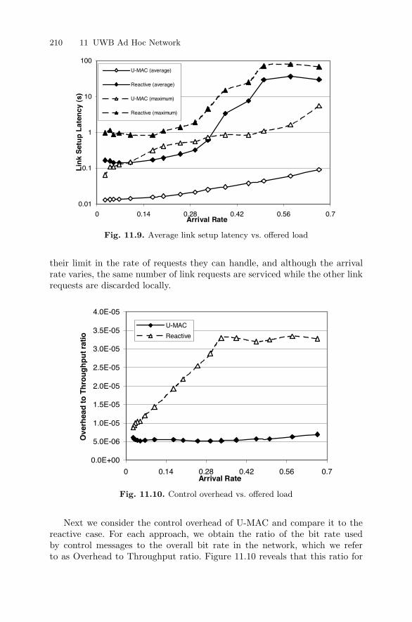
210 11 UWB Ad Hoc Network
0.01
0.1
1
10
100
0 0.14 0.28 0.42 0.56 0.7Arrival Rate
Lin
k S
etu
p L
aten
cy (
s)U-MAC (average)
Reactive (average)
U-MAC (maximum)
Reactive (maximum)
Fig. 11.9. Average link setup latency vs. offered load
their limit in the rate of requests they can handle, and although the arrivalrate varies, the same number of link requests are serviced while the other linkrequests are discarded locally.
0.0E+00
5.0E-06
1.0E-05
1.5E-05
2.0E-05
2.5E-05
3.0E-05
3.5E-05
4.0E-05
0 0.14 0.28 0.42 0.56 0.7Arrival Rate
Ove
rhea
d to
Th
rou
gh
pu
t rat
io
U-MAC
Reactive
Fig. 11.10. Control overhead vs. offered load
Next we consider the control overhead of U-MAC and compare it to thereactive case. For each approach, we obtain the ratio of the bit rate usedby control messages to the overall bit rate in the network, which we referto as Overhead to Throughput ratio. Figure 11.10 reveals that this ratio for
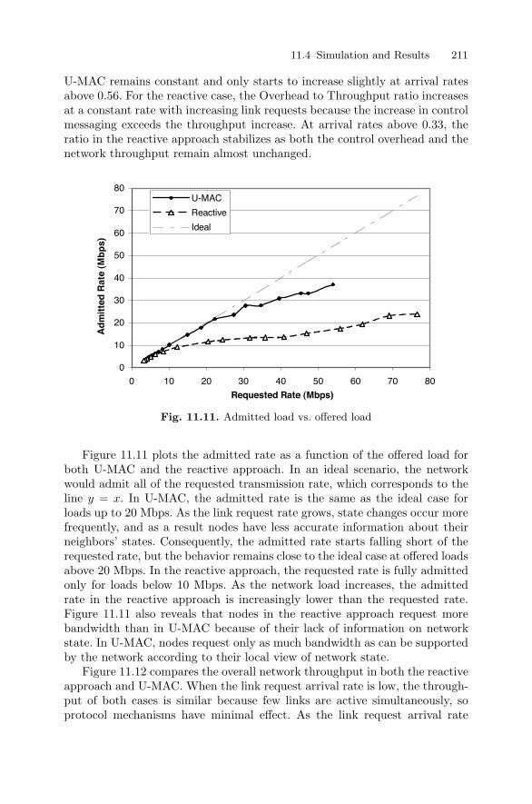
11.4 Simulation and Results 211
U-MAC remains constant and only starts to increase slightly at arrival ratesabove 0.56. For the reactive case, the Overhead to Throughput ratio increasesat a constant rate with increasing link requests because the increase in controlmessaging exceeds the throughput increase. At arrival rates above 0.33, theratio in the reactive approach stabilizes as both the control overhead and thenetwork throughput remain almost unchanged.
0
10
20
30
40
50
60
70
80
0 10 20 30 40 50 60 70 80
Requested Rate (Mbps)
Ad
mit
ted
Rat
e (M
bp
s)
U-MAC
Reactive
Ideal
Fig. 11.11. Admitted load vs. offered load
Figure 11.11 plots the admitted rate as a function of the offered load forboth U-MAC and the reactive approach. In an ideal scenario, the networkwould admit all of the requested transmission rate, which corresponds to theline y = x. In U-MAC, the admitted rate is the same as the ideal case forloads up to 20 Mbps. As the link request rate grows, state changes occur morefrequently, and as a result nodes have less accurate information about theirneighbors’ states. Consequently, the admitted rate starts falling short of therequested rate, but the behavior remains close to the ideal case at offered loadsabove 20 Mbps. In the reactive approach, the requested rate is fully admittedonly for loads below 10 Mbps. As the network load increases, the admittedrate in the reactive approach is increasingly lower than the requested rate.Figure 11.11 also reveals that nodes in the reactive approach request morebandwidth than in U-MAC because of their lack of information on networkstate. In U-MAC, nodes request only as much bandwidth as can be supportedby the network according to their local view of network state.
Figure 11.12 compares the overall network throughput in both the reactiveapproach and U-MAC. When the link request arrival rate is low, the through-put of both cases is similar because few links are active simultaneously, soprotocol mechanisms have minimal effect. As the link request arrival rate
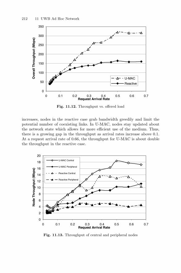
212 11 UWB Ad Hoc Network
0
50
100
150
200
250
300
350
0 0.1 0.2 0.3 0.4 0.5 0.6 0.7Request Arrival Rate
Ove
rall
Th
rou
gh
pu
t (M
bp
s)
U-MAC
Reactive
Fig. 11.12. Throughput vs. offered load
increases, nodes in the reactive case grab bandwidth greedily and limit thepotential number of coexisting links. In U-MAC, nodes stay updated aboutthe network state which allows for more efficient use of the medium. Thus,there is a growing gap in the throughput as arrival rates increase above 0.1.At a request arrival rate of 0.66, the throughput for U-MAC is about doublethe throughput in the reactive case.
0
2
4
6
8
10
12
14
16
18
20
0 0.1 0.2 0.3 0.4 0.5 0.6 0.7Request Arrival Rate
No
de
Th
rou
gh
pu
t (M
bp
s)
U-MAC Central
U-MAC Peripheral
Reactive Central
Reactive Peripheral
Fig. 11.13. Throughput of central and peripheral nodes

11.4 Simulation and Results 213
Figure 11.14 plots both the admitted link rate and the requested link rateas functions of the link request arrival rate for U-MAC and the reactive ap-proach. In the reactive approach, the requested link rate is independent ofnetwork state, so it does not vary with network load. As a result, the gapbetween admitted and requested link rates grows with network load, and sta-bilizes for link arrival rates above 0.3. In U-MAC, nodes adapt their requestedlink rate to the interference and number of active links in the network for newlink requests. The requested link rate is generally admitted for link requestarrival rates up to 0.25. For link request arrival rates between 0.25 and 0.5,there is a growing gap between the requested and admitted link rates. Thisindicates that nodes make less accurate local rate and power assignments dueto a higher rate of change in network state. However, the gap between therequested and admitted rate stabilizes for arrival rates between 0.5 and 0.66,which indicates that the portion of inaccurate rate and power assignmentsremains the same for those loads.
0
1
2
3
4
5
6
7
8
0 0.1 0.2 0.3 0.4 0.5 0.6 0.7Request Arrival Rate
Rat
e p
er L
ink
(Mb
ps)
U-MAC requested
U-MAC admitted
Reactive requested
Reactive admitted
Fig. 11.14. Rate per link vs. request arrival rate
Finally, Fig. 11.13 compares the sustained throughput of a node centralto the topology and a node on the periphery versus the link request arrivalrate. At low arrival rates, the gap between the throughput values of the twonodes is narrow regardless of MAC protocol mechanisms. As the arrival rateincreases, both nodes exhibit higher throughput, but the gap increases indi-cating that nodes central to the topology grab more bandwidth as the trafficload increases. The gap stabilizes for a link request arrival rate of about 0.5,where network throughput starts to saturate.
The gap in throughput between the 2 nodes is due to the difference intheir average distances from other nodes in the network. Decreasing the δ
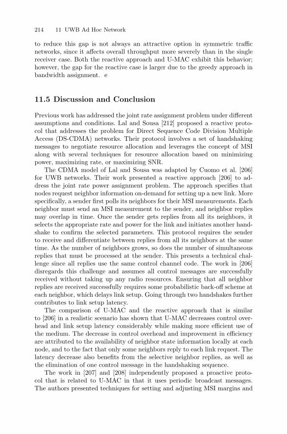
214 11 UWB Ad Hoc Network
to reduce this gap is not always an attractive option in symmetric trafficnetworks, since it affects overall throughput more severely than in the singlereceiver case. Both the reactive approach and U-MAC exhibit this behavior;however, the gap for the reactive case is larger due to the greedy approach inbandwidth assignment. e
11.5 Discussion and Conclusion
Previous work has addressed the joint rate assignment problem under differentassumptions and conditions. Lal and Sousa [212] proposed a reactive proto-col that addresses the problem for Direct Sequence Code Division MultipleAccess (DS-CDMA) networks. Their protocol involves a set of handshakingmessages to negotiate resource allocation and leverages the concept of MSIalong with several techniques for resource allocation based on minimizingpower, maximizing rate, or maximizing SNR.
The CDMA model of Lal and Sousa was adapted by Cuomo et al. [206]for UWB networks. Their work presented a reactive approach [206] to ad-dress the joint rate power assignment problem. The approach specifies thatnodes request neighbor information on-demand for setting up a new link. Morespecifically, a sender first polls its neighbors for their MSI measurements. Eachneighbor must send an MSI measurement to the sender, and neighbor repliesmay overlap in time. Once the sender gets replies from all its neighbors, itselects the appropriate rate and power for the link and initiates another hand-shake to confirm the selected parameters. This protocol requires the senderto receive and differentiate between replies from all its neighbors at the sametime. As the number of neighbors grows, so does the number of simultaneousreplies that must be processed at the sender. This presents a technical chal-lenge since all replies use the same control channel code. The work in [206]disregards this challenge and assumes all control messages are successfullyreceived without taking up any radio resources. Ensuring that all neighborreplies are received successfully requires some probabilistic back-off scheme ateach neighbor, which delays link setup. Going through two handshakes furthercontributes to link setup latency.
The comparison of U-MAC and the reactive approach that is similarto [206] in a realistic scenario has shown that U-MAC decreases control over-head and link setup latency considerably while making more efficient use ofthe medium. The decrease in control overhead and improvement in efficiencyare attributed to the availability of neighbor state information locally at eachnode, and to the fact that only some neighbors reply to each link request. Thelatency decrease also benefits from the selective neighbor replies, as well asthe elimination of one control message in the handshaking sequence.
The work in [207] and [208] independently proposed a proactive proto-col that is related to U-MAC in that it uses periodic broadcast messages.The authors presented techniques for setting and adjusting MSI margins and
11.5 Discussion and Conclusion 215
simulation results for access probabilities under different medium conditions.U-MAC further expands these ideas in 2 directions. First, U-MAC dynami-cally sets the hello message period to adapt the degree of state changes atnodes in order to avoid unnecessary state advertisements. Second, the proto-col in [207] and [208] specifies that a node setting up a link requires repliesfrom all neighbors. In U-MAC, only the subset of the neighbors that do notagree with the link parameters send replies, which is similar to the selectivereject (SREJ) concept in [212]. As a result, U-MAC reduces control overheadand link setup latency.
In addition, our work on U-MAC provides the first comparative studyof reactive and proactive approaches to the joint rate and power assignmentproblem in UWB. The study reveals that the proactive approach doubles net-work throughput under high traffic conditions. Our other simulation study ad-dresses fair access between nodes at varying distances from a common receiver,and explores the tradeoff between achieving maximum network throughputand promoting fair access to individual nodes. The results reveal that thereis a radius of fair access for each receiver within which all nodes achieve com-parable throughput. The MSI margin δ in U-MAC controls the radius of fairaccess and determines the balance between fair access to the receiver andoverall network throughput.
One direction for future research is to integrate multihop links into ourprotocol. Using information provided by hello messages, nodes can make localdecisions on least-cost paths to a particular destination [175].
Another issue for future investigation is the effect of mobility on the pro-tocol. The protocol framework provides measures of positional reliability, butour simulations only consider stationary nodes. It would be interesting to ex-plore techniques for using UWB’s radar capability to keep track of mobilenodes, and to study the impact of mobility on the hello message period andthe resulting protocol behavior.
Finally, coupling UWB’s positioning capability with directional anten-nas [217] can reduce power consumption since the receiver captures most ofthe transmitted power. Once a sender knows the receiver’s location, it candirect the antenna beam towards the receiver. Smart antennas [218], whichhave been considered for UWB transmissions [219,220], are directional anten-nas that can physically steer themselves towards the receiver. We can modifyU-MAC to operate with smart antennas by considering interference in eachsector around the receiver independently. We expect that the modified proto-col would enable more simultaneous links, provided that the links are evenlydistributed in all sectors.
The design philosophy of U-MAC also addresses the cross-layer designchallenges from Section 7.3.3. Instead of providing a short-term solution toa specific problem, U-MAC’s design adopts a forward-looking perspective forUWB networks through the extended cost function in Appendix A, which en-ables the incorporation of additional performance metrics into configurationdecisions. The cost function provides a modular and structured tool that can

216 11 UWB Ad Hoc Network
be tuned by different application to customize network behavior. The MSImargin is another tunable parameter in U-MAC that controls network per-formance. MSI margin controls the ROF around each node, which determinesthe radius within which all neighbors can have fair access to the channel.
In sum, we have presented a new proactive and adaptive MAC protocol forUWB networks called U-MAC that relies on cross-layer information sharing.U-MAC provides well-defined parameters to control the fairness/throughputtradeoff while reducing control overhead and connection latency. Because theperformance goals of U-MAC inherently cut across traditional layers, the pa-rameters that control the behavior of U-MAC originate at the application,network, MAC, and physical layers. The performance evaluation in this chap-ter has revealed the importance of information sharing across these traditionallayer boundaries for providing custom performance guarantees in UWB ad hocnetworks.
12
Acoustic Underwater Sensor Network
Acoustic technology has been established as the exclusive technology thatprovides robust underwater communications for military and civilian appli-cations. One particular civilian application of interest is the deployment ofunderwater acoustic sensor networks. The main challenges of deploying sucha network are the cost and the limited battery resources of individual sensornodes. Thus, this case study aims at maximizing the network lifetime andminimizing of power consumption of underwater sensor networks. This chap-ter applies Jurdak’s cross-layer framework to an underwater acoustic sensornetwork for monitoring of a watershed in order to achieve network longevitythrough cross-layer interaction and internode collaboration. Figure 12.1 showsthe customized framework for this case study. The focus of this chapter is thedevelopment of the optimization algorithm that maximizes battery life andminimizes energy consumption for an underwater sensor network. The opti-mization algorithm uses the following state parameters to estimate networklifetime: (1) internode distance; (2) transmission frequency; (3) sampling fre-quency; and (4) number of descendants in the routing tree. Transmission fre-quency and internode distances are both physical layer aspects. The samplingfrequency is an application layer aspect, and the number of descendants inthe routing tree is a network layer aspect. The local and neighborhood stateinformation can be employed locally at each node to dynamically select theappropriate transmission frequency.
12.1 Introduction
Wireless acoustic communication is based on the modulation of sound wavesin frequency, time, amplitude, phase, or position in order to embed data into
Portions reprinted, with permission, from (R. Jurdak, C. V. Lopes and P. Baldi.Battery Lifetime Estimation and Optimization for Underwater Sensor Networks.Sensor Network Operations, Wiley/IEEE Press, pp. 397–429, May, 2006.) c©2006Wiley-IEEE
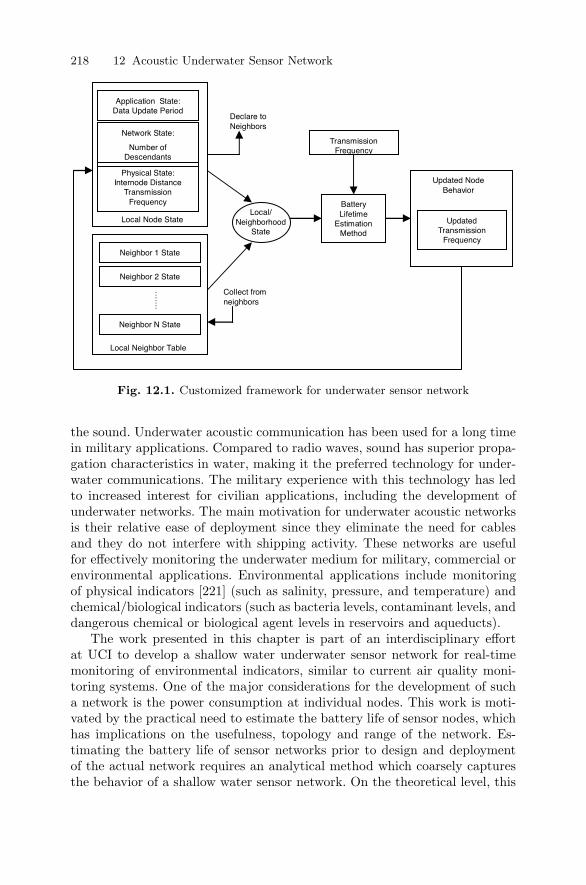
218 12 Acoustic Underwater Sensor Network
Application State: Data Update Period
Network State:
Number of Descendants
Physical State: Internode Distance
Transmission Frequency
Neighbor 1 State
Neighbor 2 State
Neighbor N State
Local Node State
.……
Local Neighbor Table
Collect from neighbors
Local/ Neighborhood
State
Declare to Neighbors
Battery Lifetime
Estimation Method
Transmission Frequency
Updated Node Behavior
Updated Transmission
Frequency
Fig. 12.1. Customized framework for underwater sensor network
the sound. Underwater acoustic communication has been used for a long timein military applications. Compared to radio waves, sound has superior propa-gation characteristics in water, making it the preferred technology for under-water communications. The military experience with this technology has ledto increased interest for civilian applications, including the development ofunderwater networks. The main motivation for underwater acoustic networksis their relative ease of deployment since they eliminate the need for cablesand they do not interfere with shipping activity. These networks are usefulfor effectively monitoring the underwater medium for military, commercial orenvironmental applications. Environmental applications include monitoringof physical indicators [221] (such as salinity, pressure, and temperature) andchemical/biological indicators (such as bacteria levels, contaminant levels, anddangerous chemical or biological agent levels in reservoirs and aqueducts).
The work presented in this chapter is part of an interdisciplinary effortat UCI to develop a shallow water underwater sensor network for real-timemonitoring of environmental indicators, similar to current air quality moni-toring systems. One of the major considerations for the development of sucha network is the power consumption at individual nodes. This work is moti-vated by the practical need to estimate the battery life of sensor nodes, whichhas implications on the usefulness, topology and range of the network. Es-timating the battery life of sensor networks prior to design and deploymentof the actual network requires an analytical method which coarsely capturesthe behavior of a shallow water sensor network. On the theoretical level, this
12.2 Related 219
work is driven by the need to develop a generic method for battery lifetimeestimation that combines both the networking and medium-specific aspectsin sensor networks.
Most of the existing work has focused on modeling the battery lifetime ofsensor networks in air [222,223]. The goals of the work in this chapter are:
• To provide an estimation method for network battery lifetime specific tothe conditions of underwater acoustic sensor networks
• To propose topology-dependent optimizations for power• To show how the estimation method fits in our framework and to evaluate
the benefits of the optimizations for a typical shallow water sensor network
The remainder of this chapter is as follows. Section 12.2 provides the neces-sary background and reviews previous related work that addresses the networklifetime issue. Section 12.3 introduces the steps of the estimation method. Sec-tion 12.4 presents the topology-specific optimizations for power consumption.Section 12.5 shows how local decisions based on topology information can es-timate the global network battery life and power consumption, through twotopologies that are representative of shallow water network scenarios. Sec-tion 12.6 discusses the analytical results and concludes the chapter.
12.2 Related
Interest in underwater acoustics dates back to the early 20th century whensonar waves were used to detect icebergs [11]. Later, the military startedusing underwater acoustics for detecting submarines [11] and mines [12,224].Underwater acoustic applications further extended to seafloor imaging [225],object localization and tracking [226], and data communication [11] for oceanexploration and management of coastal areas. The previous experiences withunderwater acoustics have led to the design of underwater sensor networksthat include a large number of sensors and perform long-term monitoring ofthe underwater environment [227]. In underwater sensor networks, the issueof limited battery resources at the sensors is particularly important becauseof the difficulty and cost of recharging sensor batteries once the network isdeployed.
In the recent literature, several approaches address estimation and opti-mization of the lifetime of energy-constrained networks. In the context of un-derwater networks, Fruehauf and Rice [228] propose the use of steerable direc-tional acoustic transducers for signal transmission and reception in underwaternodes to reduce the energy consumption and thus prolong the lifetime of anode. Among other approaches that apply to more general energy-constrainednetworks, Tilaky et al. [229] assess the tradeoffs involved in the design andtopology of sensor networks. Marsan et al. [230] consider techniques to maxi-mize the lifetime of a Bluetooth network by optimizing network topology, andargue that their optimization techniques are also applicable to general ad hoc
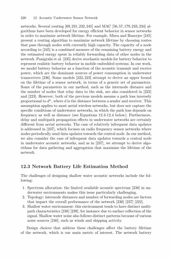
220 12 Acoustic Underwater Sensor Network
networks. Several routing [69,231,232,245] and MAC [56,57,179,233,234] al-gorithms have been developed for energy efficient behavior in sensor networksin order to maximize network lifetime. For example, Misra and Banerjee [245]present a routing algorithm to maximize network lifetime by choosing routesthat pass through nodes with currently high capacity. The capacity of a nodeaccording to [245] is a combined measure of the remaining battery energy andthe estimated energy spent in reliably forwarding data of other nodes in thenetwork. Panigrahi et al. [235] derive stochastic models for battery behavior torepresent realistic battery behavior in mobile embedded systems. In our work,we model battery behavior as a function of the acoustic transmit and receivepower, which are the dominant sources of power consumption in underwatertransceivers [236]. Some models [222, 223] attempt to derive an upper boundon the lifetime of a sensor network, in terms of a generic set of parameters.Some of the parameters in our method, such as the internode distance andthe number of nodes that relay data to the sink, are also considered in [222]and [223]. However, both of the previous models assume a path loss inverselyproportional to dn, where d is the distance between a sender and receiver. Thisassumption applies to most aerial wireless networks, but does not capture thespecific conditions of underwater networks, in which the path loss depends onfrequency as well as distance (see Equations 12.3-12.4 below). Furthermore,delay and multipath propagation effects in underwater networks are certainlydifferent from aerial networks. The case of relatively infrequent data updatesis addressed in [237], which focuses on radio frequency sensor networks wherenodes periodically send data updates towards the central node. In our method,we also consider the case of infrequent data updates towards a central nodein underwater acoustic networks, and as in [237], we attempt to derive algo-rithms for data gathering and aggregation that maximize the lifetime of thenetwork.
12.3 Network Battery Life Estimation Method
The challenges of designing shallow water acoustic networks include the fol-lowing:
1. Spectrum allocation: the limited available acoustic spectrum [238] in un-derwater environments makes this issue particularly challenging.
2. Topology: internode distances and number of forwarding nodes are factorsthat impact the overall performance of the network [230] [237] [222].
3. Shallow water environment: this environment tends to have distinct multi-path characteristics [238] [239], for instance due to surface reflection of thesignal. Shallow water noise also follows distinct patterns because of variousnoise sources [240], such as winds and shipping activity.
Design choices that address these challenges affect the battery lifetimeof the network, which is our main metric of interest. The network battery
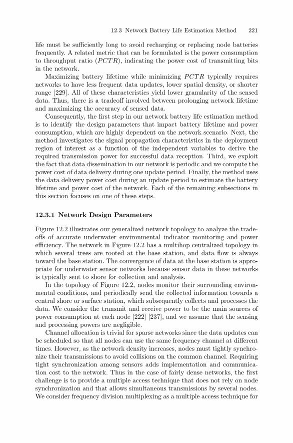
12.3 Network Battery Life Estimation Method 221
life must be sufficiently long to avoid recharging or replacing node batteriesfrequently. A related metric that can be formulated is the power consumptionto throughput ratio (PCTR), indicating the power cost of transmitting bitsin the network.
Maximizing battery lifetime while minimizing PCTR typically requiresnetworks to have less frequent data updates, lower spatial density, or shorterrange [229]. All of these characteristics yield lower granularity of the senseddata. Thus, there is a tradeoff involved between prolonging network lifetimeand maximizing the accuracy of sensed data.
Consequently, the first step in our network battery life estimation methodis to identify the design parameters that impact battery lifetime and powerconsumption, which are highly dependent on the network scenario. Next, themethod investigates the signal propagation characteristics in the deploymentregion of interest as a function of the independent variables to derive therequired transmission power for successful data reception. Third, we exploitthe fact that data dissemination in our network is periodic and we compute thepower cost of data delivery during one update period. Finally, the method usesthe data delivery power cost during an update period to estimate the batterylifetime and power cost of the network. Each of the remaining subsections inthis section focuses on one of these steps.
12.3.1 Network Design Parameters
Figure 12.2 illustrates our generalized network topology to analyze the trade-offs of accurate underwater environmental indicator monitoring and powerefficiency. The network in Figure 12.2 has a multihop centralized topology inwhich several trees are rooted at the base station, and data flow is alwaystoward the base station. The convergence of data at the base station is appro-priate for underwater sensor networks because sensor data in these networksis typically sent to shore for collection and analysis.
In the topology of Figure 12.2, nodes monitor their surrounding environ-mental conditions, and periodically send the collected information towards acentral shore or surface station, which subsequently collects and processes thedata. We consider the transmit and receive power to be the main sources ofpower consumption at each node [222] [237], and we assume that the sensingand processing powers are negligible.
Channel allocation is trivial for sparse networks since the data updates canbe scheduled so that all nodes can use the same frequency channel at differenttimes. However, as the network density increases, nodes must tightly synchro-nize their transmissions to avoid collisions on the common channel. Requiringtight synchronization among sensors adds implementation and communica-tion cost to the network. Thus in the case of fairly dense networks, the firstchallenge is to provide a multiple access technique that does not rely on nodesynchronization and that allows simultaneous transmissions by several nodes.We consider frequency division multiplexing as a multiple access technique for
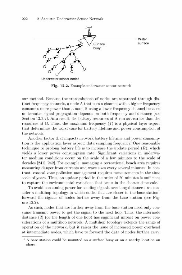
222 12 Acoustic Underwater Sensor Network
Surface buoy
Underwater sensor nodes
Water surface
Fig. 12.2. Example underwater sensor network
our method. Because the transmissions of nodes are separated through dis-tinct frequency channels, a node A that uses a channel with a higher frequencyconsumes more power than a node B using a lower frequency channel becauseunderwater signal propagation depends on both frequency and distance (seeSection 12.3.2). As a result, the battery resources at A run out earlier than theresources at B. Thus, the maximum frequency (f) is a physical layer aspectthat determines the worst case for battery lifetime and power consumption ofthe network.
Another factor that impacts network battery lifetime and power consump-tion is the application layer aspect: data sampling frequency. One reasonabletechnique to prolong battery life is to increase the update period (R), whichyields a lower power consumption rate. Significant variations in underwa-ter medium conditions occur on the scale of a few minutes to the scale ofdecades [241] [242]. For example, managing a recreational beach area requiresmeasuring danger from currents and wave sizes every several minutes. In con-trast, coastal zone pollution management requires measurements in the timescale of years. Thus, an update period in the order of 20 minutes is sufficientto capture the environmental variations that occur in the shorter timescale.
To avoid consuming power for sending signals over long distances, we con-sider a multihop topology in which nodes that are closer to the base station1
forward the signals of nodes further away from the base station (see Fig-ure 12.2).
As such, nodes that are further away from the base station need only con-sume transmit power to get the signal to the next hop. Thus, the internodedistance (d) (or the length of one hop) has significant impact on power con-siderations of a multihop network. A multihop topology extends the range ofoperation of the network, but it raises the issue of increased power overheadat intermediate nodes, which have to forward the data of nodes further away.1 A base station could be mounted on a surface buoy or on a nearby location on
shore
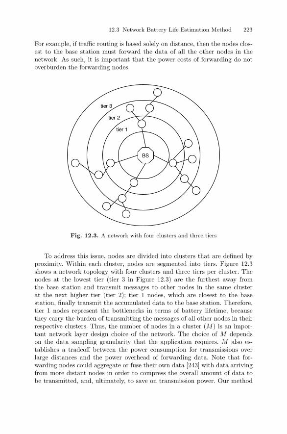
12.3 Network Battery Life Estimation Method 223
For example, if traffic routing is based solely on distance, then the nodes clos-est to the base station must forward the data of all the other nodes in thenetwork. As such, it is important that the power costs of forwarding do notoverburden the forwarding nodes.
tier 3
tier 2
tier 1
BS
Fig. 12.3. A network with four clusters and three tiers
To address this issue, nodes are divided into clusters that are defined byproximity. Within each cluster, nodes are segmented into tiers. Figure 12.3shows a network topology with four clusters and three tiers per cluster. Thenodes at the lowest tier (tier 3 in Figure 12.3) are the furthest away fromthe base station and transmit messages to other nodes in the same clusterat the next higher tier (tier 2); tier 1 nodes, which are closest to the basestation, finally transmit the accumulated data to the base station. Therefore,tier 1 nodes represent the bottlenecks in terms of battery lifetime, becausethey carry the burden of transmitting the messages of all other nodes in theirrespective clusters. Thus, the number of nodes in a cluster (M) is an impor-tant network layer design choice of the network. The choice of M dependson the data sampling granularity that the application requires. M also es-tablishes a tradeoff between the power consumption for transmissions overlarge distances and the power overhead of forwarding data. Note that for-warding nodes could aggregate or fuse their own data [243] with data arrivingfrom more distant nodes in order to compress the overall amount of data tobe transmitted, and, ultimately, to save on transmission power. Our method

224 12 Acoustic Underwater Sensor Network
does not consider aggregation, and thus presents a conservative estimate ofthe power consumption at the forwarding nodes.
In sum, we identified four important network design parameters that im-pact the battery lifetime and power consumption of an underwater sensornetwork: (1) the transmission frequency f ; (2) the update period R; (3) theaverage signal transmission distance d; and (4) the number of nodes in a clus-ter M . Our framework can use these parameters in local algorithms to adapteach node’s behavior in line with the global optimization goal of maximizingnetwork lifetime.
12.3.2 Underwater Acoustics Fundamentals
This section covers the fundamentals of underwater acoustics, enabling theestimation of transmit and receive powers for underwater communication.
The Passive Sonar Equation
The passive sonar equation [11] characterizes the signal to noise ratio (SNR)of an emitted underwater signal at the receiver:
SNR = SL − TL − NL + DI (12.1)
where SL is the source level, TL is the transmission loss, NL is the noiselevel, and DI is the directivity index. All the quantities in Equation 12.1are in dB re µPa, where the reference value of 1 µPa amounts to 0.67 ×10⁻²² Watts/cm2 [11]. In the rest of the chapter, we use the shorthand nota-tion of dB to signify dB re µPa.
Factors contributing to the noise level NL in shallow water networks in-clude waves, shipping traffic, wind level, biological noise, seaquakes and vol-canic activity, and the impact of each of these factors on NL depends on theparticular setting. For instance, shipping activity may dominate noise figuresin bays or ports, while water currents are the primary noise source in rivers.For the purpose of this analysis, we examined several studies of shallow wa-ter noise measurements under different conditions [240] [11]. As a result, weconsider an average value for the ambient noise level NL to be 70 dB as a rep-resentative shallow water case. We also consider a target SNR of 15 dB [11]at the receiver.
The directivity index DI for our network is zero because we assume om-nidirectional hydrophones. Note that this is another conservative assumption,since using a directive hydrophone as described in [228] reduces power con-sumption.
Through the above assumptions, we can express the source level SL in-tensity as a function of TL only:
SL = TL + 85 (12.2)
in dB.
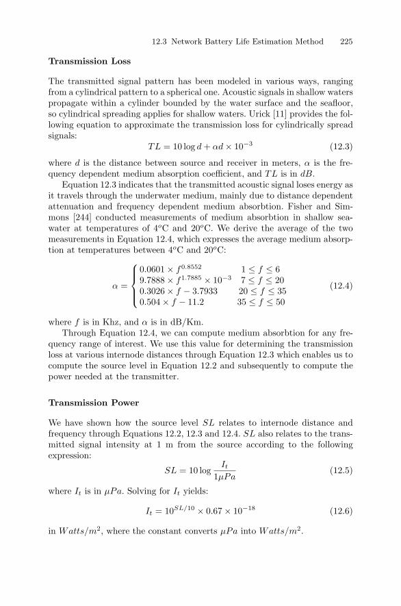
12.3 Network Battery Life Estimation Method 225
Transmission Loss
The transmitted signal pattern has been modeled in various ways, rangingfrom a cylindrical pattern to a spherical one. Acoustic signals in shallow waterspropagate within a cylinder bounded by the water surface and the seafloor,so cylindrical spreading applies for shallow waters. Urick [11] provides the fol-lowing equation to approximate the transmission loss for cylindrically spreadsignals:
TL = 10 log d + αd × 10−3 (12.3)
where d is the distance between source and receiver in meters, α is the fre-quency dependent medium absorption coefficient, and TL is in dB.
Equation 12.3 indicates that the transmitted acoustic signal loses energy asit travels through the underwater medium, mainly due to distance dependentattenuation and frequency dependent medium absorbtion. Fisher and Sim-mons [244] conducted measurements of medium absorbtion in shallow sea-water at temperatures of 4oC and 20oC. We derive the average of the twomeasurements in Equation 12.4, which expresses the average medium absorp-tion at temperatures between 4oC and 20oC:
α =
⎧⎪⎪⎨⎪⎪⎩
0.0601 × f0.8552 1 ≤ f ≤ 69.7888 × f1.7885 × 10−3 7 ≤ f ≤ 200.3026 × f − 3.7933 20 ≤ f ≤ 350.504 × f − 11.2 35 ≤ f ≤ 50
(12.4)
where f is in Khz, and α is in dB/Km.Through Equation 12.4, we can compute medium absorbtion for any fre-
quency range of interest. We use this value for determining the transmissionloss at various internode distances through Equation 12.3 which enables us tocompute the source level in Equation 12.2 and subsequently to compute thepower needed at the transmitter.
Transmission Power
We have shown how the source level SL relates to internode distance andfrequency through Equations 12.2, 12.3 and 12.4. SL also relates to the trans-mitted signal intensity at 1 m from the source according to the followingexpression:
SL = 10 logIt
1µPa(12.5)
where It is in µPa. Solving for It yields:
It = 10SL/10 × 0.67 × 10−18 (12.6)
in Watts/m2, where the constant converts µPa into Watts/m2.
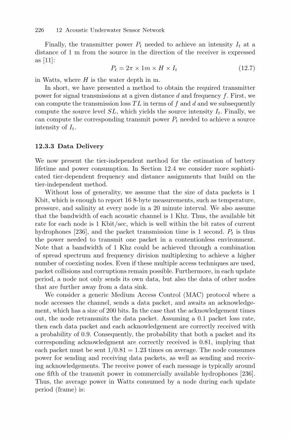
226 12 Acoustic Underwater Sensor Network
Finally, the transmitter power Pt needed to achieve an intensity It at adistance of 1 m from the source in the direction of the receiver is expressedas [11]:
Pt = 2π × 1m × H × It (12.7)
in Watts, where H is the water depth in m.In short, we have presented a method to obtain the required transmitter
power for signal transmissions at a given distance d and frequency f . First, wecan compute the transmission loss TL in terms of f and d and we subsequentlycompute the source level SL, which yields the source intensity It. Finally, wecan compute the corresponding transmit power Pt needed to achieve a sourceintensity of It.
12.3.3 Data Delivery
We now present the tier-independent method for the estimation of batterylifetime and power consumption. In Section 12.4 we consider more sophisti-cated tier-dependent frequency and distance assignments that build on thetier-independent method.
Without loss of generality, we assume that the size of data packets is 1Kbit, which is enough to report 16 8-byte measurements, such as temperature,pressure, and salinity at every node in a 20 minute interval. We also assumethat the bandwidth of each acoustic channel is 1 Khz. Thus, the available bitrate for each node is 1 Kbit/sec, which is well within the bit rates of currenthydrophones [236], and the packet transmission time is 1 second. Pt is thusthe power needed to transmit one packet in a contentionless environment.Note that a bandwidth of 1 Khz could be achieved through a combinationof spread spectrum and frequency division multiplexing to achieve a highernumber of coexisting nodes. Even if these multiple access techniques are used,packet collisions and corruptions remain possible. Furthermore, in each updateperiod, a node not only sends its own data, but also the data of other nodesthat are further away from a data sink.
We consider a generic Medium Access Control (MAC) protocol where anode accesses the channel, sends a data packet, and awaits an acknowledge-ment, which has a size of 200 bits. In the case that the acknowledgement timesout, the node retransmits the data packet. Assuming a 0.1 packet loss rate,then each data packet and each acknowledgement are correctly received witha probability of 0.9. Consequently, the probability that both a packet and itscorresponding acknowledgment are correctly received is 0.81, implying thateach packet must be sent 1/0.81 = 1.23 times on average. The node consumespower for sending and receiving data packets, as well as sending and receiv-ing acknowledgements. The receive power of each message is typically aroundone fifth of the transmit power in commercially available hydrophones [236].Thus, the average power in Watts consumed by a node during each updateperiod (frame) is:
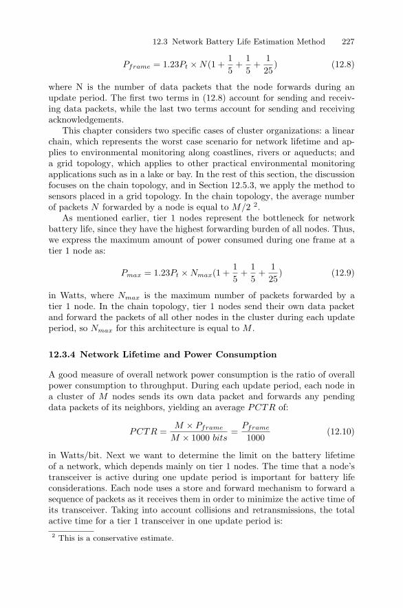
12.3 Network Battery Life Estimation Method 227
Pframe = 1.23Pt × N(1 +15
+15
+125
) (12.8)
where N is the number of data packets that the node forwards during anupdate period. The first two terms in (12.8) account for sending and receiv-ing data packets, while the last two terms account for sending and receivingacknowledgements.
This chapter considers two specific cases of cluster organizations: a linearchain, which represents the worst case scenario for network lifetime and ap-plies to environmental monitoring along coastlines, rivers or aqueducts; anda grid topology, which applies to other practical environmental monitoringapplications such as in a lake or bay. In the rest of this section, the discussionfocuses on the chain topology, and in Section 12.5.3, we apply the method tosensors placed in a grid topology. In the chain topology, the average numberof packets N forwarded by a node is equal to M/2 2.
As mentioned earlier, tier 1 nodes represent the bottleneck for networkbattery life, since they have the highest forwarding burden of all nodes. Thus,we express the maximum amount of power consumed during one frame at atier 1 node as:
Pmax = 1.23Pt × Nmax(1 +15
+15
+125
) (12.9)
in Watts, where Nmax is the maximum number of packets forwarded by atier 1 node. In the chain topology, tier 1 nodes send their own data packetand forward the packets of all other nodes in the cluster during each updateperiod, so Nmax for this architecture is equal to M .
12.3.4 Network Lifetime and Power Consumption
A good measure of overall network power consumption is the ratio of overallpower consumption to throughput. During each update period, each node ina cluster of M nodes sends its own data packet and forwards any pendingdata packets of its neighbors, yielding an average PCTR of:
PCTR =M × Pframe
M × 1000 bits=
Pframe
1000(12.10)
in Watts/bit. Next we want to determine the limit on the battery lifetimeof a network, which depends mainly on tier 1 nodes. The time that a node’stransceiver is active during one update period is important for battery lifeconsiderations. Each node uses a store and forward mechanism to forward asequence of packets as it receives them in order to minimize the active time ofits transceiver. Taking into account collisions and retransmissions, the totalactive time for a tier 1 transceiver in one update period is:2 This is a conservative estimate.

228 12 Acoustic Underwater Sensor Network
Ttotal = 1.23(Nmax +Nmax
5) (12.11)
in seconds.The next step is selecting a power source. We consider that we have 3 off-
the-shelf 9V, 1.2 Amp-Hour batteries at each node. The total energy availableat each node is:
Et = 3 × 9 × 1.2 = 32.4 (12.12)
in V ·A · hour. The total active time of a transceiver is therefore the ratio ofthe total energy to the power consumed in one frame:
Tactive =Et
Pframe=
32.4Pframe
(12.13)
in hours. A node’s transceiver is only active for a fraction of the time ineach update period of R seconds. Therefore, the battery lifetime of a node isexpressed by:
Tlifetime =Tactive
Ttotal× R
24(12.14)
in days, where R is in seconds.
12.4 Topology-Dependent Optimizations
The tier-independent battery life and power consumption estimation methodin Section 12.3 treats all network nodes equally, by assuming all internode dis-tances are the same and by assigning frequency values randomly. However, thetier-independent method disregards the fact that tier 1 nodes carry a heavierpower burden than other nodes. Consequently, applying measures that favortier 1 nodes can yield improvements in battery life and power consumption.For this purpose, we propose an enhancement to the tier-independent batterylife and power consumption estimation method, in which each node can lo-cally select its own transmission frequency based on its logical position in therouting tree. This optimization is similar to the consideration of number ofdescendants in the routing tree for setting listening modes in the case studyof Chapter 10.
Equations 12.3 and 12.4 indicate that the transmission loss increases athigher frequencies, which implies that nodes using high frequencies must trans-mit acoustic signals at higher power. Thus, nodes at tier 1 can choose lowestfrequency band, and nodes at each subsequent tier can select the next higherfrequency band. Within this rationale, nodes at the lowest tier select the high-est frequency band. This assignment allows nodes with higher forwarding loadto use lower frequencies and thus save power.
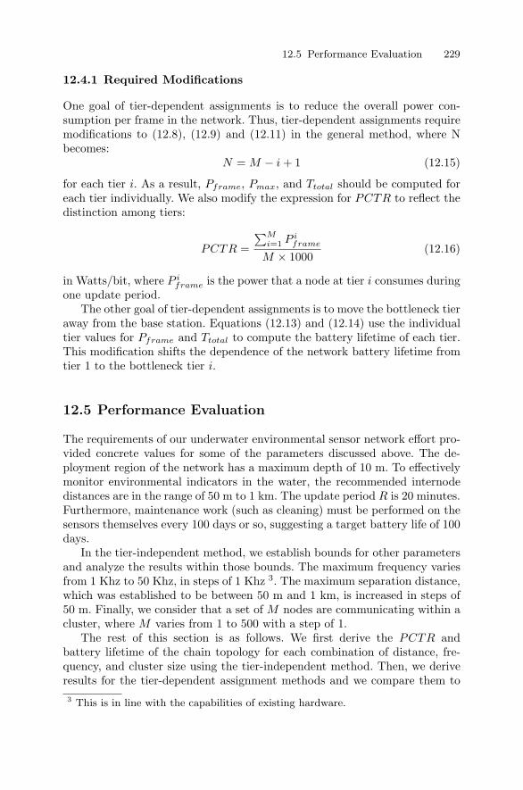
12.5 Performance Evaluation 229
12.4.1 Required Modifications
One goal of tier-dependent assignments is to reduce the overall power con-sumption per frame in the network. Thus, tier-dependent assignments requiremodifications to (12.8), (12.9) and (12.11) in the general method, where Nbecomes:
N = M − i + 1 (12.15)
for each tier i. As a result, Pframe, Pmax, and Ttotal should be computed foreach tier individually. We also modify the expression for PCTR to reflect thedistinction among tiers:
PCTR =
∑Mi=1 P i
frame
M × 1000(12.16)
in Watts/bit, where P iframe is the power that a node at tier i consumes during
one update period.The other goal of tier-dependent assignments is to move the bottleneck tier
away from the base station. Equations (12.13) and (12.14) use the individualtier values for Pframe and Ttotal to compute the battery lifetime of each tier.This modification shifts the dependence of the network battery lifetime fromtier 1 to the bottleneck tier i.
12.5 Performance Evaluation
The requirements of our underwater environmental sensor network effort pro-vided concrete values for some of the parameters discussed above. The de-ployment region of the network has a maximum depth of 10 m. To effectivelymonitor environmental indicators in the water, the recommended internodedistances are in the range of 50 m to 1 km. The update period R is 20 minutes.Furthermore, maintenance work (such as cleaning) must be performed on thesensors themselves every 100 days or so, suggesting a target battery life of 100days.
In the tier-independent method, we establish bounds for other parametersand analyze the results within those bounds. The maximum frequency variesfrom 1 Khz to 50 Khz, in steps of 1 Khz 3. The maximum separation distance,which was established to be between 50 m and 1 km, is increased in steps of50 m. Finally, we consider that a set of M nodes are communicating within acluster, where M varies from 1 to 500 with a step of 1.
The rest of this section is as follows. We first derive the PCTR andbattery lifetime of the chain topology for each combination of distance, fre-quency, and cluster size using the tier-independent method. Then, we deriveresults for the tier-dependent assignment methods and we compare them to3 This is in line with the capabilities of existing hardware.
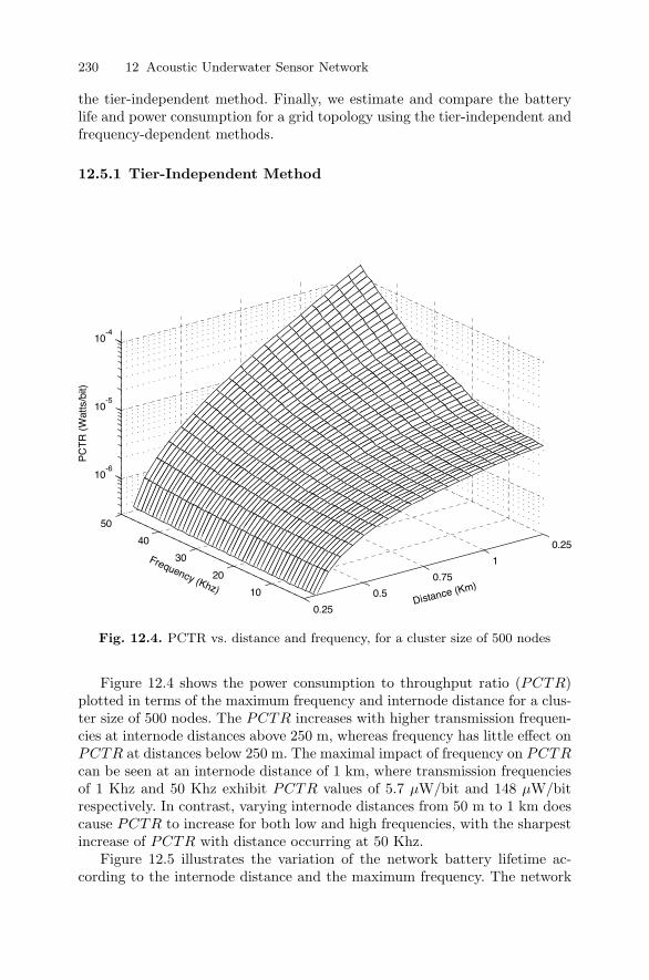
230 12 Acoustic Underwater Sensor Network
the tier-independent method. Finally, we estimate and compare the batterylife and power consumption for a grid topology using the tier-independent andfrequency-dependent methods.
12.5.1 Tier-Independent Method
0.25
0.5
0.75
1
0.25
10
20
30
40
50
10-6
10-5
10-4
Distance (Km)
Frequency (Khz)
PC
TR
(W
atts
/bit)
Fig. 12.4. PCTR vs. distance and frequency, for a cluster size of 500 nodes
Figure 12.4 shows the power consumption to throughput ratio (PCTR)plotted in terms of the maximum frequency and internode distance for a clus-ter size of 500 nodes. The PCTR increases with higher transmission frequen-cies at internode distances above 250 m, whereas frequency has little effect onPCTR at distances below 250 m. The maximal impact of frequency on PCTRcan be seen at an internode distance of 1 km, where transmission frequenciesof 1 Khz and 50 Khz exhibit PCTR values of 5.7 µW/bit and 148 µW/bitrespectively. In contrast, varying internode distances from 50 m to 1 km doescause PCTR to increase for both low and high frequencies, with the sharpestincrease of PCTR with distance occurring at 50 Khz.
Figure 12.5 illustrates the variation of the network battery lifetime ac-cording to the internode distance and the maximum frequency. The network
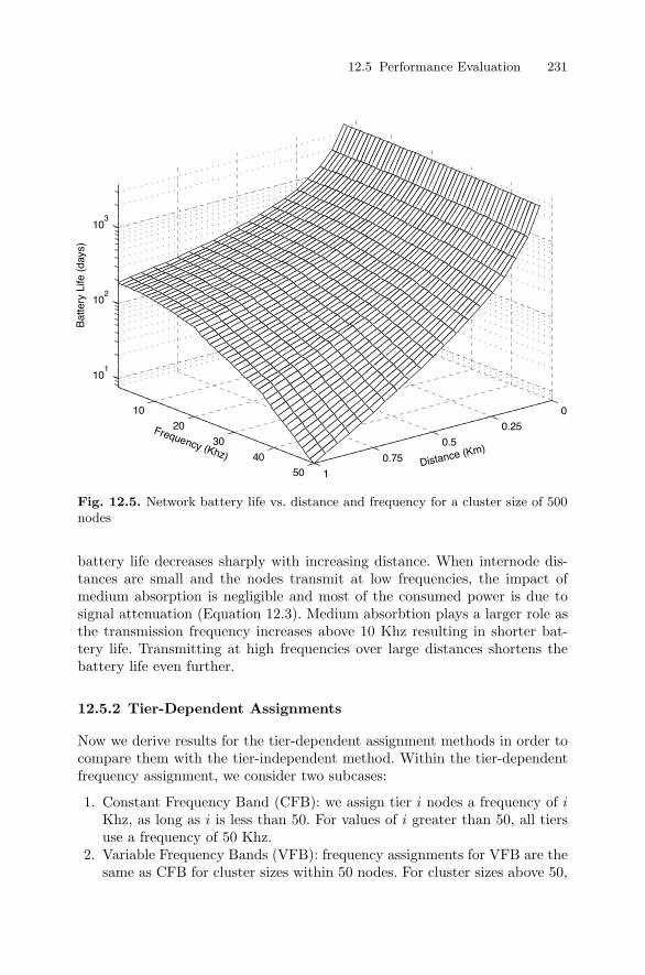
12.5 Performance Evaluation 231
0
0.25
0.5
0.75
1
10
20
30
40
50
101
102
103
Distance (Km)
Frequency (Khz)
Bat
tery
Life
(da
ys)
Fig. 12.5. Network battery life vs. distance and frequency for a cluster size of 500nodes
battery life decreases sharply with increasing distance. When internode dis-tances are small and the nodes transmit at low frequencies, the impact ofmedium absorption is negligible and most of the consumed power is due tosignal attenuation (Equation 12.3). Medium absorbtion plays a larger role asthe transmission frequency increases above 10 Khz resulting in shorter bat-tery life. Transmitting at high frequencies over large distances shortens thebattery life even further.
12.5.2 Tier-Dependent Assignments
Now we derive results for the tier-dependent assignment methods in order tocompare them with the tier-independent method. Within the tier-dependentfrequency assignment, we consider two subcases:
1. Constant Frequency Band (CFB): we assign tier i nodes a frequency of iKhz, as long as i is less than 50. For values of i greater than 50, all tiersuse a frequency of 50 Khz.
2. Variable Frequency Bands (VFB): frequency assignments for VFB are thesame as CFB for cluster sizes within 50 nodes. For cluster sizes above 50,
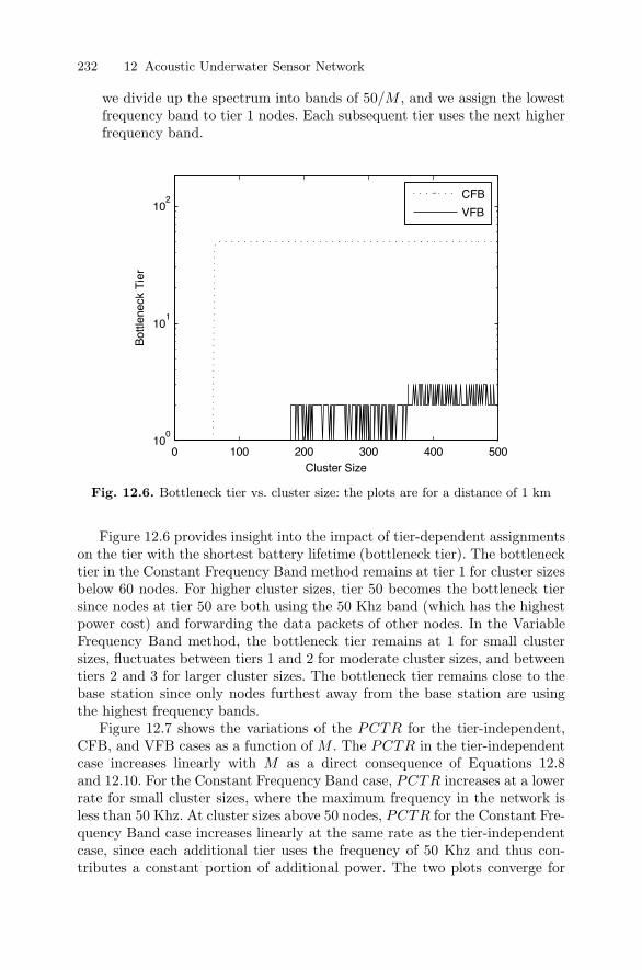
232 12 Acoustic Underwater Sensor Network
we divide up the spectrum into bands of 50/M , and we assign the lowestfrequency band to tier 1 nodes. Each subsequent tier uses the next higherfrequency band.
0 100 200 300 400 50010
0
101
102
Cluster Size
Bot
tlene
ck T
ier
CFB
VFB
Fig. 12.6. Bottleneck tier vs. cluster size: the plots are for a distance of 1 km
Figure 12.6 provides insight into the impact of tier-dependent assignmentson the tier with the shortest battery lifetime (bottleneck tier). The bottlenecktier in the Constant Frequency Band method remains at tier 1 for cluster sizesbelow 60 nodes. For higher cluster sizes, tier 50 becomes the bottleneck tiersince nodes at tier 50 are both using the 50 Khz band (which has the highestpower cost) and forwarding the data packets of other nodes. In the VariableFrequency Band method, the bottleneck tier remains at 1 for small clustersizes, fluctuates between tiers 1 and 2 for moderate cluster sizes, and betweentiers 2 and 3 for larger cluster sizes. The bottleneck tier remains close to thebase station since only nodes furthest away from the base station are usingthe highest frequency bands.
Figure 12.7 shows the variations of the PCTR for the tier-independent,CFB, and VFB cases as a function of M . The PCTR in the tier-independentcase increases linearly with M as a direct consequence of Equations 12.8and 12.10. For the Constant Frequency Band case, PCTR increases at a lowerrate for small cluster sizes, where the maximum frequency in the network isless than 50 Khz. At cluster sizes above 50 nodes, PCTR for the Constant Fre-quency Band case increases linearly at the same rate as the tier-independentcase, since each additional tier uses the frequency of 50 Khz and thus con-tributes a constant portion of additional power. The two plots converge for
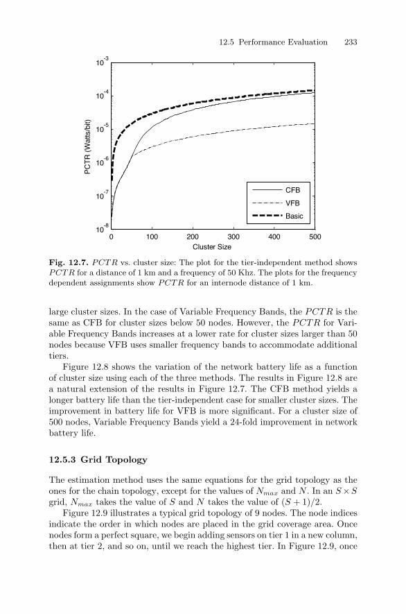
12.5 Performance Evaluation 233
0 100 200 300 400 50010
-8
10-7
10-6
10-5
10-4
10-3
Cluster Size
PC
TR
(W
atts
/bit)
CFB
VFB
Basic
Fig. 12.7. PCTR vs. cluster size: The plot for the tier-independent method showsPCTR for a distance of 1 km and a frequency of 50 Khz. The plots for the frequencydependent assignments show PCTR for an internode distance of 1 km.
large cluster sizes. In the case of Variable Frequency Bands, the PCTR is thesame as CFB for cluster sizes below 50 nodes. However, the PCTR for Vari-able Frequency Bands increases at a lower rate for cluster sizes larger than 50nodes because VFB uses smaller frequency bands to accommodate additionaltiers.
Figure 12.8 shows the variation of the network battery life as a functionof cluster size using each of the three methods. The results in Figure 12.8 area natural extension of the results in Figure 12.7. The CFB method yields alonger battery life than the tier-independent case for smaller cluster sizes. Theimprovement in battery life for VFB is more significant. For a cluster size of500 nodes, Variable Frequency Bands yield a 24-fold improvement in networkbattery life.
12.5.3 Grid Topology
The estimation method uses the same equations for the grid topology as theones for the chain topology, except for the values of Nmax and N . In an S×Sgrid, Nmax takes the value of S and N takes the value of (S + 1)/2.
Figure 12.9 illustrates a typical grid topology of 9 nodes. The node indicesindicate the order in which nodes are placed in the grid coverage area. Oncenodes form a perfect square, we begin adding sensors on tier 1 in a new column,then at tier 2, and so on, until we reach the highest tier. In Figure 12.9, once
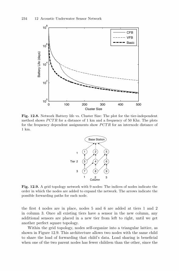
234 12 Acoustic Underwater Sensor Network
0 100 200 300 400 50010
0
102
104
106
108
Cluster Size
Bat
tery
Life
(da
ys)
CFB
VFB
Basic
Fig. 12.8. Network Battery life vs. Cluster Size: The plot for the tier-independentmethod shows PCTR for a distance of 1 km and a frequency of 50 Khz. The plotsfor the frequency dependent assignments show PCTR for an internode distance of1 km.
2 5
4 6
1
3
8 97
Base Station
Tier
1
2
31 2Column
3
Fig. 12.9. A grid topology network with 9 nodes: The indices of nodes indicate theorder in which the nodes are added to expand the network. The arrows indicate thepossible forwarding paths for each node.
the first 4 nodes are in place, nodes 5 and 6 are added at tiers 1 and 2in column 3. Once all existing tiers have a sensor in the new column, anyadditional sensors are placed in a new tier from left to right, until we getanother perfect square topology.
Within the grid topology, nodes self-organize into a triangular lattice, asshown in Figure 12.9. This architecture allows two nodes with the same childto share the load of forwarding that child’s data. Load sharing is beneficialwhen one of the two parent nodes has fewer children than the other, since the
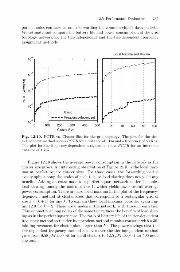
12.5 Performance Evaluation 235
parent nodes can take turns in forwarding the common child’s data packets.We estimate and compare the battery life and power consumption of the gridtopology network for the tier-independent and the tier-dependent frequencyassignment methods.
0 100 200 300 400 50010
-8
10-7
10-6
10-5
10-4
Cluster Size
PC
TR
(W
atts
/bit)
20 40 60 80 100
Basic
Frequency-dependent
Local Maxima and Minima
Fig. 12.10. PCTR vs. Cluster Size for the grid topology: The plot for the tier-independent method shows PCTR for a distance of 1 km and a frequency of 50 Khz.The plot for the frequency-dependent assignments show PCTR for an internodedistance of 1 km.
Figure 12.10 shows the average power consumption in the network as thecluster size grows. An interesting observation of Figure 12.10 is the local max-ima at perfect square cluster sizes. For those cases, the forwarding load isevenly split among the nodes of each tier, so load sharing does not yield anybenefits. Adding an extra node to a perfect square network at tier 1 enablesload sharing among the nodes of tier 1, which yields lower overall averagepower consumption. There are also local maxima in the plot of the frequency-dependent method at cluster sizes that correspond to a rectangular grid ofsize k × (k + 1) for any k. To explain these local maxima, consider again Fig-ure 12.9 for k = 2. There are 6 nodes in the network, with three in each tier.This symmetry among nodes of the same tier reduces the benefits of load shar-ing as in the perfect square case. The ratio of battery life of the tier-dependentfrequency method to the tier-independent method remains constant with a 30-fold improvement for cluster sizes larger than 50. The power savings that thetier-dependent frequency method achieves over the tier-independent methodgrow from 0.58 µWatts/bit for small clusters to 12.5 µWatts/bit for 500 nodeclusters.
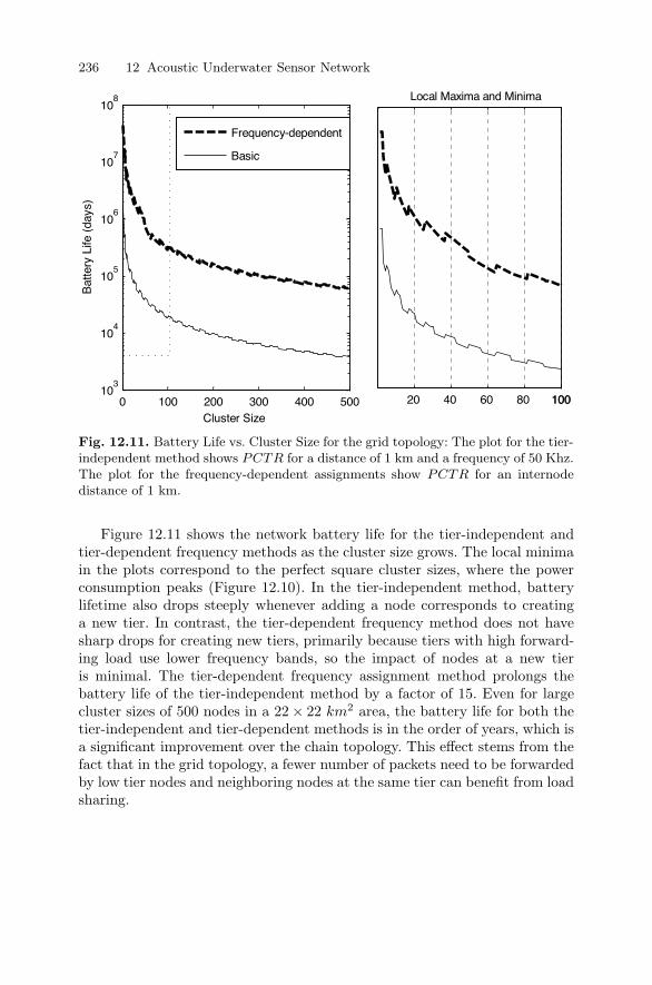
236 12 Acoustic Underwater Sensor Network
0 100 200 300 400 50010
3
104
105
106
107
108
Cluster Size
Bat
tery
Life
(da
ys)
20 40 60 80 100100
Frequency-dependent
Basic
Local Maxima and Minima
Fig. 12.11. Battery Life vs. Cluster Size for the grid topology: The plot for the tier-independent method shows PCTR for a distance of 1 km and a frequency of 50 Khz.The plot for the frequency-dependent assignments show PCTR for an internodedistance of 1 km.
Figure 12.11 shows the network battery life for the tier-independent andtier-dependent frequency methods as the cluster size grows. The local minimain the plots correspond to the perfect square cluster sizes, where the powerconsumption peaks (Figure 12.10). In the tier-independent method, batterylifetime also drops steeply whenever adding a node corresponds to creatinga new tier. In contrast, the tier-dependent frequency method does not havesharp drops for creating new tiers, primarily because tiers with high forward-ing load use lower frequency bands, so the impact of nodes at a new tieris minimal. The tier-dependent frequency assignment method prolongs thebattery life of the tier-independent method by a factor of 15. Even for largecluster sizes of 500 nodes in a 22 × 22 km2 area, the battery life for both thetier-independent and tier-dependent methods is in the order of years, which isa significant improvement over the chain topology. This effect stems from thefact that in the grid topology, a fewer number of packets need to be forwardedby low tier nodes and neighboring nodes at the same tier can benefit from loadsharing.
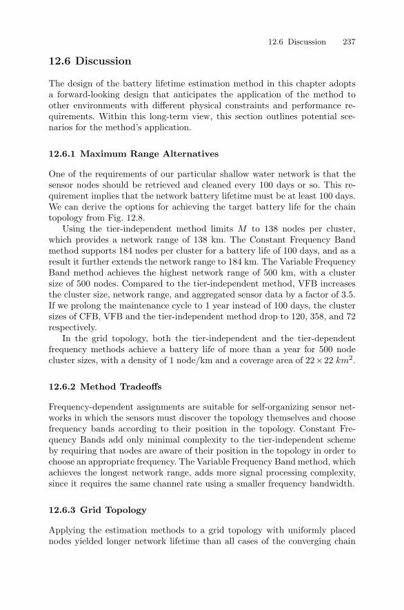
12.6 Discussion 237
12.6 Discussion
The design of the battery lifetime estimation method in this chapter adoptsa forward-looking design that anticipates the application of the method toother environments with different physical constraints and performance re-quirements. Within this long-term view, this section outlines potential sce-narios for the method’s application.
12.6.1 Maximum Range Alternatives
One of the requirements of our particular shallow water network is that thesensor nodes should be retrieved and cleaned every 100 days or so. This re-quirement implies that the network battery lifetime must be at least 100 days.We can derive the options for achieving the target battery life for the chaintopology from Fig. 12.8.
Using the tier-independent method limits M to 138 nodes per cluster,which provides a network range of 138 km. The Constant Frequency Bandmethod supports 184 nodes per cluster for a battery life of 100 days, and as aresult it further extends the network range to 184 km. The Variable FrequencyBand method achieves the highest network range of 500 km, with a clustersize of 500 nodes. Compared to the tier-independent method, VFB increasesthe cluster size, network range, and aggregated sensor data by a factor of 3.5.If we prolong the maintenance cycle to 1 year instead of 100 days, the clustersizes of CFB, VFB and the tier-independent method drop to 120, 358, and 72respectively.
In the grid topology, both the tier-independent and the tier-dependentfrequency methods achieve a battery life of more than a year for 500 nodecluster sizes, with a density of 1 node/km and a coverage area of 22×22 km2.
12.6.2 Method Tradeoffs
Frequency-dependent assignments are suitable for self-organizing sensor net-works in which the sensors must discover the topology themselves and choosefrequency bands according to their position in the topology. Constant Fre-quency Bands add only minimal complexity to the tier-independent schemeby requiring that nodes are aware of their position in the topology in order tochoose an appropriate frequency. The Variable Frequency Band method, whichachieves the longest network range, adds more signal processing complexity,since it requires the same channel rate using a smaller frequency bandwidth.
12.6.3 Grid Topology
Applying the estimation methods to a grid topology with uniformly placednodes yielded longer network lifetime than all cases of the converging chain
238 12 Acoustic Underwater Sensor Network
network, which is to be expected since the chain topology represents the lowerbound on network lifetime. As mentioned earlier, networks with a grid topol-ogy are useful for environmental monitoring of lakes or bays. The estimationresults that we derived cover a maximum area of 22 × 22 km2. To apply theresults to larger areas, a relay station at the edge of each cluster can collectthe data and forward to the base station. Alternatively, the network can stilluse a single base station and simply expand cluster sizes to cover the largerarea.
12.6.4 Self-Recharging Sensors
Battery lifetime in sensor networks becomes less of an issue if there is someway of recharging battery resources at individual nodes without human in-tervention. In an underwater sensor network, nodes can derive mechanical,chemical, or solar energy from their surrounding environment. For example,nodes could absorb and store mechanical energy from water flows throughsmall windmill-like devices. Whether the benefits of such devices overweighthe cost of building them into sensor nodes remains an open issue.
12.6.5 Method Applicability
Although we applied our method to a shallow seawater network, the methodalso applies to networks at any depth and any fluid. In deeper waters, the im-pact of both distance and frequency on transmission loss changes. One obviousdistinction is that the signal undergoes spherical spreading for deeper waters,as opposed to cylindrical spreading in shallow water. Medium absorption isalso depth dependent, and several studies [246] have explored this dependencethrough measurements. Other factors, such as the noise level, should also bemodified to represent deep water environments. Applying the method to otherfluids also requires similar changes to the path loss and noise models. Finally,the network deployment setting may require other changes to the method.For instance, there is no signal spreading in pipes and the transmission lossbeyond a certain range is independent of distance.
Conclusion: In sum, we derived a method to estimate the battery lifeand power cost for underwater sensor networks. Our method first identifiesthe main independent variables (f , d, M , R) that impact network battery lifeand power consumption. Next, the method investigates the signal propagationcharacteristics in the deployment region of interest as a function of the inde-pendent variables (f and d in this case) to derive the required transmissionpower for successful data reception. Third, the transmission power estimateis combined with the relevant independent variables (M and R in this case)to compute the power cost of data delivery during one update period. Finally,the method uses the data delivery power cost during an update period toestimate the average node battery life and average network power cost.

12.6 Discussion 239
We applied this estimation method and its tier-dependent variants to a setof shallow water network scenarios which are representative of our underwa-ter sensor network effort. We found that for the chain topology, the VariableFrequency Band method maximizes network range for a given cluster size, pro-vides data samples at uniform granularity, and still achieves a comparativelylong battery life.
We also applied the method to a grid topology with uniformly placedsensors to estimate the network battery life and power consumption. Thebattery life was expectedly longer in the grid topology than the chain topology,and the tier-dependent frequency assignments prolonged battery life nearly bya factor of fifteen over the tier-independent method. Because our method isapplicable to any topology or fluid medium, researchers can adapt the methodto estimate power consumption and network battery life in the initial designand planning stages of fluid sensor networks.
13
Concluding Remarks and Future Directions
This book focuses on cross-layer design for ad hoc and sensor networks. Thefirst part of the book surveys layered approaches for these networks, while thesecond part of the book discusses explicit cross-layer design. Part III of thebook takes Jurdak’s cross-layer optimization framework as an example thatis applicable to three diverse case studies. The case studies cover both ad hocand sensor networks with diverse communication technologies (RF, UWB,and acoustics) and with diverse application requirements, including energyefficiency, network longevity, throughput maximization, fair access, and lowlatency. The applicability of Jurdak’s framework to the diverse case studieshighlights the success of synergistic approaches that provide flexibility formultiple scenarios on one hand and efficient performance for each scenario onthe other.
Where does cross-layer design for ad hoc and sensor networks go from here?The answer to this question points in several directions. Certainly, having anall-encompassing architecture for ad hoc and sensor networks that supportsrich cross-layer interactions would promote innovation in the field and widerscale deployment of ad hoc and sensor network applications. The architecturesdiscussed in Chapter 8 strive to provide such an architecture that providescross-layer information sharing through a common state repository, benefitingfrom cross-layer interactions while maintaining the interfaces of the layeredarchitecture. Existing cross-layer architectures still have some way to go beforehaving a significant impact on the development of ad hoc and sensor networks.First, most proposed architectures (except for Jurdak’s framework) targeteither ad hoc or sensor networks. Although it may limit an architecture’simpact, targeting one class of networks could lead to an acceptable balancebetween generality and performance. Another factor that limits the impact ofproposed cross-layer architectures is that most of them are still in the processof being implemented, so realizing the extent of their widespread adoptionwill be delayed.
A final issue is whether ad hoc and sensor networks require an all-encompassing architecture. If not, then designers can simply address each
242 13 Concluding Remarks and Future Directions
network scenario with a design coupling approach that combines the func-tionalities of multiple layers to improve network performance for that sce-nario. Many sensor networks could benefit from designing custom algorithmsfor each application. Because sensor networks are highly application-specificand they are typically operated by a single entity, the network user may pri-oritize performance for this unique application rather than the flexibility andinteroperability of the algorithms for more general applications. That said,the provision of an architecture still promises to provide a fertile ground forthe development and widespread deployment of more general ad hoc networkapplications and sensor network applications alike.
A
Extended Cost Function
Our framework determines the routing behavior of nodes by enabling eachnode to learn its neighborhood state and to set the routing cost of each neigh-bor according to the cost function. Our cost function has a weighted additivestructure that enables network designers to manipulate the relevance of eachcost metric by setting the metrics’ weights in the cost function.
This appendix presents an extended cost function for our sensor networkoptimization framework, adopting many metrics from the global cost functionof Baldi et al. for UWB networks. However, our cost function differs from thecost function in [175] in the following ways: (1) it assigns costs to nodes insteadof links; and (2) it groups some cost metrics from [175] into composite costmetrics that are descriptive of important sensor network aspects.
Each node locally computes the cost of a neighbor N according to theglobal cost function:
C(N) = k3C(delivery) + k4C(power)+k5C(delay) + k6C(reliability)
+k7C(interference) + k8C(other) (A.1)
where k3 − k8 are the weights of the individual cost metrics. In what follows,we briefly discuss each of the cost function metrics.
Data Delivery
One of the main goals in almost all sensor networks is efficiently deliveringsensed data to the user. In our cost function, the cost metric C(delivery)indicates the data delivery cost of a particular neighbor. Delivering data insensor networks should minimize the number of hops in the path to the datasink and maximize the quality of the links along that path. Thus, C(delivery)is a composite cost metric:
C(delivery) = k9C(hops) + k10C(quality) (A.2)
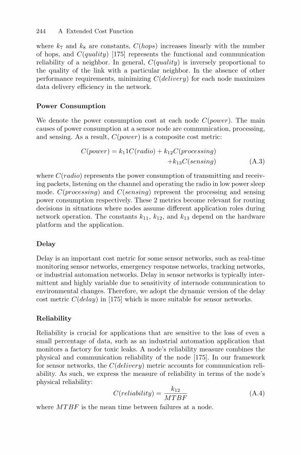
244 A Extended Cost Function
where k7 and k8 are constants, C(hops) increases linearly with the numberof hops, and C(quality) [175] represents the functional and communicationreliability of a neighbor. In general, C(quality) is inversely proportional tothe quality of the link with a particular neighbor. In the absence of otherperformance requirements, minimizing C(delivery) for each node maximizesdata delivery efficiency in the network.
Power Consumption
We denote the power consumption cost at each node C(power). The maincauses of power consumption at a sensor node are communication, processing,and sensing. As a result, C(power) is a composite cost metric:
C(power) = k11C(radio) + k12C(processing)+k13C(sensing) (A.3)
where C(radio) represents the power consumption of transmitting and receiv-ing packets, listening on the channel and operating the radio in low power sleepmode. C(processing) and C(sensing) represent the processing and sensingpower consumption respectively. These 2 metrics become relevant for routingdecisions in situations where nodes assume different application roles duringnetwork operation. The constants k11, k12, and k13 depend on the hardwareplatform and the application.
Delay
Delay is an important cost metric for some sensor networks, such as real-timemonitoring sensor networks, emergency response networks, tracking networks,or industrial automation networks. Delay in sensor networks is typically inter-mittent and highly variable due to sensitivity of internode communication toenvironmental changes. Therefore, we adopt the dynamic version of the delaycost metric C(delay) in [175] which is more suitable for sensor networks.
Reliability
Reliability is crucial for applications that are sensitive to the loss of even asmall percentage of data, such as an industrial automation application thatmonitors a factory for toxic leaks. A node’s reliability measure combines thephysical and communication reliability of the node [175]. In our frameworkfor sensor networks, the C(delivery) metric accounts for communication reli-ability. As such, we express the measure of reliability in terms of the node’sphysical reliability:
C(reliability) =k12
MTBF(A.4)
where MTBF is the mean time between failures at a node.

A Extended Cost Function 245
Interference
Another important cost metric in some networks is interference. This metricis especially crucial in sensor networks that use spread spectrum commu-nication technology. Our framework here aims to maintain generality withregard to communication technology, so we adopt the interference cost metricC(interference) from [175] without specifying it quantitatively.
Other Metrics
Our cost function enables the inclusion of additional cost metrics, such asthe cost of setting up a new link [175] or the cost of maintaining fairness. Inaddition, networks with multiple traffic classes may give priority to high ratenodes, which necessitates adapting the routing cost accordingly. The abovemetrics as well as any other metrics can be included in the metric C(other).
References
1. ISO. “Open Systems Interconnection–Basic Reference Model” ISO 7498.2. T. Socolofsky and C. Kale. A TCP/IP Tutorial. Request for Comments: 1180,
1991. available: http://rfc.sunsite.dk/rfc/rfc1180.html.a3. Global System for Mobile Communications. ETSI standard. available:
http://www.etsi.org.4. National Archives and Records Administration. U.S. GLOBAL POSITIONING
SYSTEM POLICY. March 29, 1996.5. IEEE 802.11 WG. “Wireless Lan Medium Access Control (MAC) and Physical
Layer (PHY) Specifications”, Standard. 1999.6. “The Bluetooth Special Interst Group,” 1999.7. Mica Mote Series. Crossbow Technology Inc. available:
http://www.xbow.com/Products/productdetails.aspx?sid=72.8. Zigbee Alliance. available: www.zigbee.org.9. RFID Journal. available: www.rfidjournal.com.
10. M. Z. Win and R. Scholtz. “Impulse Radio: How it Works”. IEEE Communi-cations Letters, 2(1), 1998.
11. R. J. Urick. Principles of Underwater Sound. McGraw-Hill, 1983.12. J. Groen, J.C. Sabel and A. Htet. “Synthetic aperture processing techniques
applied to rail experiments with a mine hunting sonar”. In Proc. UDT Europe,2001.
13. C. V. Lopes and P. Aguiar. “Acoustic Modems for Ubiquitous Computing,”IEEE Pervasive Computing, Mobile and Ubiquitous Systems, Summer 2003.
14. R. Jurdak, C. V. Lopes and P. Baldi. Battery Lifetime Estimation and Optimiza-tion for Underwater Sensor Networks. Sensor Network Operations, Wiley/IEEEPress, pp. 397–429, May, 2006.
15. R. Jurdak, C.V. Lopes, and P. Baldi. “An Acoustic Identification Scheme ofLocation Systems,” In Proc. ICPS’04, Beirut, Lebanon, 2004.
16. A. Mandal, C. V. Lopes, T. Givargis, A. Haghighat, R. Jurdak, and P. Baldi.“Beep: 3D Indoor Positioning Using Audible Sound,” Proceedings of the IEEEConsumer Communications and Networking Conference (CCNC05). Las Vegas,Nevada, 2005.
17. A. J. Viterbi. CDMA : Principles of Spread Spectrum Communication. PrenticeHall, 1995.
18. J. Schiller. Mobile Communications, Addison-Wesley, 2000.
248 References
19. A. Chandra, V. Gummalla and J. O. Limb. “Wireless Medium AccessControl Protocols.” IEEE Communications Surveys [Online]. available:http://www.comsoc.org/pubs/surveys. Second Quarter 2000.
20. M. J. Crocker. Handbook of Acoustics, Wiley-Interscience, 1998.21. P. Baldi, L. De Nardis, and M. G. Di Benedetto. “Modelling and Optimization
of UWB Communication Networks Through a Flexible Cost Function,” IEEEJournal on Selected Areas in Communications, 20(9):1733–1744, 2002.
22. C. V. Lopes and P. Aguiar. “Acoustic Modems for Ubiquitous Computing,”IEEE Pervasive Computing, Mobile and Ubiquitous Systems, Summer 2003.
23. M. Weiser. “The computer for the 21st century,” Scientific American, 265(3:94–104, 1991.
24. L. Kleinrock and F. A. Tobagi. “Packet Switching in Radio Channels: Part I-Carrier Sense Multiple-Access Models and their Throughput-Delay Character-istics,” IEEE Transactions on Communications, 23(12):1400–1416, 1975.
25. F. A. Tobagi and L. Kleinrock. “Packet Switching in Radio Channels: PartII-The Hidden Terminal Problem in Carrier Sense Multiple-Access and theBusy-Tone Solution,” IEEE Transactions on Communications, 23(12):1417–1433, 1975.
26. “IEEE/ANSI Standard:Carrier Sense Multiple Access with Collision Detection,”1985.
27. D. J. Goodman, R. A. Valenzuela, K. T. Gayliard, and B. Ramamurthi, “PacketReservation Multiple Access for Local Wireless Communications,” In VehicularTechnology Conference, pp. 701–706, IEEE, 1988.
28. P. Karn. “MACA - A New Channel Access Protocol for Packet Radio,” InARRL/CRRL Amateur Radio Ninth Computer Networking Conference, pp.134–140, 1990.
29. V. Bharghavan, A. Demers, S. Shenker, and L. Zhang. “MACAW: A MediaAccess Protocol for Wireless LAN’s,” In ACM SIGCOMM94, pp. 212–225,ACM, 1994.
30. C. L. Fullmer and J. J. Garcia-Luna-Aceves. “Floor Acquisition Multiple Access(FAMA) for Packet-Radio Networks,” In Conference on Applications, Technolo-gies, Architectures and Protocols for Computer Communication (SIGCOMM),pp. 262–273, 1995.
31. F. Talucci, M. Gerla, and L. Fratta. “MACA-BI (MACA By Invitation) A Re-ceiver Oriented Access Protocol for Wireless Multihop Networks,” In ’Waves ofthe Year 2000’ PIMRC ’97 The 8th IEEE International Symposium on Personal,Indoor and Mobile Radio Communications, volume 2, pp. 435–439, 1997.
32. C. Zu and M. S. Corson. “A Five-Phase Reservation Protocol (FPRP) forMobile Ad Hoc Networks,” In Seventeenth Annual Joint Conference of theIEEE Computer and Communications Societies, volume 1, pp. 322–331, 1998.
33. S. Singh and C.S. Raghavendra. “Power Efficient MAC Protocol for MultihopRadio Networks,” In The Ninth IEEE International Symposium on Personal,Indoor and Mobile Radio Communications, volume 1, 1998.
34. M. J. Markowski and A.S. Sethi. “Fully Distributed Wireless MAC Transmissionof Real-Time Data,” In Fourth IEEE Real-Time Technology and ApplicationsSymposium, pp. 49–57, 1998.
35. Z. Tang and J. J. Garcia-Luna-Aceves, “Hop Reservation Multiple Access(HRMA) for Multichannel Packet Radio Networks,” In International Confer-ence on Computer Communications and Networks, pp. 388–395, 1998.
References 249
36. A. Nasipuri, J. Zhuang, and S. R. Das. “A Multichannel CSMA MAC Protocolfor Multihop Wireless Networks,” In Wireless Communications and NetworkingConference, pp. 1402–1406. IEEE, 1999.
37. L. Bononi, M. Conti, and L. Donatiello. “Distributed Contention Control Mech-anism for Power Saving in Random-Access Ad-Hoc Wireless Local Area Net-works,” In International Workshop on Mobile Multimedia Communications, pp.114–123, IEEE, 1999.
38. J. J. Garcia-Luna-Aceves and A. Tzamaloukas. “Reversing the Collision-Avoidance Handshake in Wireless Networks,” In ACM/IEEE Mobicom ’99,1999.
39. I. Chlamtac, et al. “ADAPT: A Dynamically Self-Adjusting Media Access Con-trol Protocol for Ad Hoc Networks,” In IEEE Globecom, 1999.
40. Z. Tang and J. J. Garcia-Luna-Aceves. “A Protocol for Topology-DependentTransmission Scheduling in Wireless Networks,” In IEEE WCNC, 1999.
41. K. T. Jin and D. H. Cho. “A MAC Algorithm for Energy-Limited Ad-HocNetworks,” In 52nd Vehicular Technology Conference, volume 1, pp. 219–222,IEEE, 2000.
42. C. K. Toh, V. Vassiliou, G. Guichal, and C. H. Shih. “MARCH: A MediumAccess Control Protocol for Multihop Wireless Ad Hoc Networks,” In MIL-COM 21st Century Military Communications Conference, volume 1, pp. 512–516, 2000.
43. A. Tzamaloukas and J. J. Garcia-Luna-Aceves. “A Channel-Hopping Proto-col for Ad-Hoc Networks,” In Ninth International Conference on ComputerCommunications and Networks, pp. 142–147, 2000.
44. C. W. Ahn, C. G. Kang, and Y. Z. Cho. “Soft Reservation Multiple Access withPriority Assignment (SRMA/PA): A Novel MAC Protocol for QoS-GuaranteedIntegrated Services in Mobile Ad-hoc Networks,” In 52nd Vehicular TechnologyConference, volume 2, pp. 942–947, IEEE, 2000.
45. Y. C. Tseng, S. L. Wu, C. Y. Lin, and J. P. Sheu, “A Multi-Channel MAC Pro-tocol with Power Control for Multi-Hop Mobile Ad Hoc Networks,” In Interna-tional Conference on Distributed Computing Systems Workshop, pp. 419–424,2001.
46. J. Monks, J. P. Ebert, A. Wolisz, and W. M. Hwu, “A Study of the EnergySaving and Capacity Improvement Potential of Power Control in Multi-HopWireless Networks,” In 26th Annual IEEE Conference on Local Computer Net-works, pp. 550–559, 2001.
47. H. Hassanein and A. Safwat. “Virtual Base Stations For Wireless Mobile Ad HocCommunications: An Infrastructure for the Infrastructure-less,” InternationalJournal of Communication Systems, (14):763–782, 2001.
48. J. Kim and N. Bambos. “Power-Efficient MAC Scheme using Channel Prob-ing in Multi-rate Wireless Ad Hoc Networks,” In IEEE Vehicular TechnologyConference, volume 4, pp. 2380–2384, 2002.
49. D. Lal, R. Toshniwal, R. Radhakrishnan, D. P. Agrawal, and J. Caffery. “A NovelMAC Layer Protocol for Space Division Multiple Access in Wireless Ad HocNetworks,” In Eleventh International Conference on Computer Communicationsand Networks, pp. 614–619, 2002.
50. Y. C. Tseng, C. M. Chao, S. L. Wu, and J. P. Sheu. “Dynamic Channel Al-location with Location Awareness for Multi-Hop Mobile Ad Hoc Networks,”Computer Communications, 25:676–688, 2002.
250 References
51. K. T. Jin and D. H. Cho. “Multi-Code MAC for Multi-Hop Wireless Ad hoc Net-works,” In Vehicular Technology Conference, volume 2, pp. 1100–1104, IEEE,2002.
52. M. Chatterjee, S. K. Das, and D. Turgut. “WCA: A Weighted Clustering Algo-rithm for Mobile Ad Hoc Networks,” Cluster Computing, (5):193–204, 2002.
53. Z. J. Haas and J. Deng. “Dual Busy Tone Multiple Access (DBTMA)- A Mul-tiple Access Control Scheme for Ad Hoc Networks,” IEEE Transactions onCommunications, 50(6):975–985, 2002.
54. R. R. Choudhury, X. Yang, R. Ramanathan, and N. H. Vaidya. “Using Direc-tional Antennas for Medium Access Control in Ad Hoc Networks,” In Mobicom,2002.
55. S. Jiang, J. Rao, D. He, X. Ling, and C. C. Ko. “A Simple Distributed PRMAfor MANETs,” IEEE Transactions on Vehicular Technology, 51:293–305, 2002.
56. J. Polastre, J. Hill, and D. Culler. “Versatile Low Power Media Access forWireless Sensor Networks”. Proceedings of ACM SenSys, 2004.
57. W. Ye, J. Heidemann and D. Estrin. “An Energy-Efficient MAC Protocol forWireless Sensor Networks”. In Proc. IEEE Infocom, 2002.
58. T. Van Dam and K. Langendoen. “An adaptive energy-efficient MAC protocolfor wireless sensor networks”. In Proc. 1st international conference on Embeddednetworked sensor systems, 171-180, 2003.
59. Royer, E.M. and Chai-Keong, T. “A Review of Current Routing Protocols forAd Hoc Mobile Wireless Networks”. IEEE Personal Communications, 6(2):46–55, 1999.
60. L. Qin and T. Kunz. “Survey on Mobile Ad Hoc Network Routing Protocols andCross-Layer Design”. Carleton University, Systems and Computer Engineering,Technical Report SCE-04-14, August 2004.
61. Q. Jiang and D. Manivannan. “Routing Protocols for Sensor Networks”. InProc. IEEE (CCNC), 2004.
62. G. Malkin. RIP Version 2 Carrying Additional Information. Request for Com-ments: 1723, 1994. available: http://www.ietf.org/rfc/rfc1723.txt.
63. M. A. Sportack. IP Routing Fundamentals. Indianapolis: Cisco Press, 1999.64. F. Baker and R. Coltun. OSPF Version 2 Management Information Base. Re-
quest for Comments: 1850, 1995. available: http://www.ietf.org/rfc/rfc1850.txt.65. Charles Perkins. “Highly Dynamic Destination-Sequenced Distance-Vector
Routing (DSDV) for Mobile Computers”. In Proc. ACM SIGCOMM’94 Con-ference on Communications Architectures, Protocols and Applications, 1994.
66. T. Clausen and P. Jacquet. “Optimized Link State Routing Pro-tocol (OLSR)”. Request for Comments: 3626, 2003. available:http://www.ietf.org/rfc/rfc3626.txt.
67. W. Heinzelmann, J. Kulik, and H. Balakrishnan. “Negotiation-based Protocolsfor Disseminating Information in Wireless Sensor Networks”. In Proc. Mobicom,1999.
68. W. Heinzelmann, A. Chandrakasan, and H. Balakrishnan. “Energy-EfficientCommunication Protocol for Wireless Microsensor Networks”. In Proc. HICSS,2000.
69. S. Lindsey and C. Raghavendra. “PEGASIS: Power-Efficient Gathering in Sen-sor Information Systems”. In Proc. ICC, 2001.
70. A. Manjeshwar and D. Agrawal. “TEEN: A Routing Protocol for EnhancedEfficiency in Wireless Sensor Networks”. In Proc. IPDPS, 2001.
References 251
71. C. Perkins, E. Belding-Royer, and S. Das. “Ad hoc On-Demand DistanceVector (AODV) Routing”. Request for Comments: 3561, 2003. available:http://www.ietf.org/rfc/rfc3561.txt.
72. Charles E. Perkins. “DSR: The Dynamic Source Routing Protocol for Multi-Hop Wireless Ad Hoc Networks”. In Ad Hoc Networking, edited by Charles E.Perkins, Chapter 5, pp. 139-172, Addison-Wesley, 2001.
73. K. Sundaresan and R. Sivakumar. “Routing in Ad-Hoc Networks with MIMILinks”. In Proc. 13th IEEE International Conference on Network Protocols(ICNP’05), November, 2005.
74. IEEE 802.11n. IEEE Standard for Enhancements for Higher Throughput. DraftStandard.
75. IEEE 802.16. IEEE Standard for Local and metropolitan area networks - Part16: Air Interface for Fixed Broadband Wireless Access Systems. Standard.available: http://standards.ieee.org/getieee802/download/802.16-2004.pdf.
76. V. D. Park and M. S. Corson. Temporally-ordered routing algorithm (tora).Internet draft RFC, version 1, 1997.
77. M. R. Pearlman and Z. J. Haas. “Determining the optimal configuration forthe zone routing protocol” IEEE J. Select. Areas Commun., vol. 6, no. 2, pp.1395-1414, Aug. 1999.
78. C. Intanagonwiwat, et al. “Directed Diffusion for Wireless Sensor Networking”.IEEE/ACM Trans. on Networking, 11:2-16, 2003.
79. D. Braginsky and D. Estrin. “Rumor Routing Algorithm for Sensor Networks”.In Proc. 1st ACM Int. Workshop on Wireless Sensor Nets and Applications,2002.
80. F. Ye, et al. “A Scalable Solution to Minimum Cost Forwarding in Large SensorNetworks”. In Proc. ICCCN, 2001.
81. P. Chowdavarapu and V.-G. Puram. “An Overview of Routing Protocols inAdHoc Networks”. Technical Report CS-90 Voice Over IP Lab, Universityof Kentucky Laboratory for Advanced Networking, December 2000. available:http://voip.netlab.uky.edu/venu/cs690/adhocprots.doc.
82. M. Jiang, J. Li, Y. C. Tay. Cluster Based Routing Protocol (CBRP). FunctionalSpecification Internet Draft, draft-ietf-manet-cbrp.txt, work in progress, June1999.
83. G. Pei, M. Gerla, X. Hong and C. C. Chiang. “A Wireless Hierarchical RoutingProtocol with Group Mobility”. In Proc. IEEE Wireless Communications andNetworking Conference, 1999.
84. G. Montenegro. Reverse Tunneling for Mobile IP, revised. Request for Com-ments: 2344, 1995. available: http://www.ietf.org/rfc/rfc2344.txt.
85. P. Bahl and V. Padmanabhan. “RADAR: An In-Building RF-Based User Lo-cation and Tracking System,” In Proc. IEEE Infocom 2000, IEEE CS Press,pp. 775-784, 2000.
86. N.B. Priyantha, A. Chakraborty, and H. Balakrishnan. “The Cricket Location-Support System,” Proc. 6th Ann. Intl Conf. Mobile Computing and Networking(Mobicom 00), ACM Press, pp. 32-43, 2000.
87. B. N. Karp, and H. T. Kung “GPSR: Greedy Perimeter Stateless Routing forWireless Networks,” In proc. ACM/IEEE International Conference on Mobilecomputing and networking (MobiCom ’00), pp. 243-254, August 2000.
88. Y.B. Ko and N. Vaidya. “Location-aided Routing (LAR) in mobile ad hocnetworks”. In Proc. ACM/IEEE International Conference on Mobile Computingand Networking, pp. 66-75, 1998.
252 References
89. J. Li, J. J. Douglas, S. J. De Coutu, D. R. Karger, R. Morris. “A ScalableLocation Service for Geographic Ad Hoc Routing,” In Proc. ACM/IEEE Inter-national Conference on Mobile Computing and Networking, pp. 120–130, 2000.
90. K. Seada, M. Zuniga, A. Helmy, and B. Krishnamachari. “Energy-Efficient For-warding Strategies for Geographic Routing in Lossy Wireless Sensor Networks”.In Proc. SenSys’04, November, 2004.
91. M. Zuniga and B. Krishnamachari. “Analyzing the Transitional Region oin LowPower Wireless Links”. In Proc IEEE SECON’04, 2004.
92. C. Perkins. Ad Hoc Networking, Addison-Wesley, December, 2000.93. E. M. Belding-Royer. “Multi-level Hierarchies for Scalable Ad hoc Routing.”
Wireless Networking (WINET), 9(5), pp. 461-478, Sept. 2003.94. Dashy, S., Bandar, S., Brown, T.X. “An on-demand minimum energy routing
protocol for a wireless ad hoc network”. ACM Mobile Computing and Commu-nication, 6(3):50-66, 2002.
95. Rodoplu, V., Meng, T.H. “Minimum Energy Mobile Wireless Networks”. InProc. IEEE International Conference on Communications, 3:1633-1693, 1998.
96. Singh, S., Woo, M., Raghavendra, C. S. “Power-aware Routing in Mobile AdHoc Networks”. In proc. MobiCom98, ACM/IEEE, pp.181–190, 1998.
97. Toh, C.K. “Maximum battery life routing to support ubiquitous mobile comput-ing in wireless ad hoc networks”. IEEE Communications Magazine, 39:138-147,2001.
98. R. C. Shah and J. M. Rabaey. “Energy Aware Routing for Low Energy Ad HocSensor Networks”. In Proc. IEEE Wireless Communications and NetworkingConference (WCNC), March 2002.
99. D. S. J. De Couto, D. Aguayo, J. Bicket, and R. Morris. “A High-ThroughputPath Metric for Multi-Hop Wireless Routing” In Proc.Mobicom’03, September2003.
100. R. Jurdak. “Modeling and Optimization of Ad Hoc and Sensor Networks,”Bren School of Information and Computer Science, University of CaliforniaIrvine. Ph.D. Dissertation. September, 2005.
101. C. Park, K. Lahiri, and A. Raghunathan. “Battery Discharge Characteristicsof Wireless Sensor Nodes: An Experimental Analysis”. In Proc. IEEE SECON,2005.
102. R. Sivakumar, P. Sinha and V. Bharghavan. “Core extraction distributedad hoc routing (CEDAR) specification,” IETF Internet draft draft-ietf-manet-cedar-spec-00.txt, 1998.
103. K. Sohrabi, J. Gao, V. Ailawadhi, and G. J. Potie. “Protocols for self-organization of a wireless sensor network,” IEEE Personal Communications,pp. 16-27, October 2000.
104. K. Akkaya and M. Younis. “An Energy-Aware QoS Routing Protocol for Wire-less Sensor Networks,” In Proc. 23rd International Conference on DistributedComputing Systems Workshops (ICDCSW’03), pp. 710, 2003.
105. S. Chen and K. NahrStedt. “Distributed Quality of Service Routing in AdHoc Networks,” IEEE Journal on Selected Areas in Communications, 17(8),pp.1488–1505, Aug. 1999.
106. D. Ganesan, R. Govindan, S. Shenker, and D. Estrin. “Highly Resilient Energy-Efficient Multipath Routing in Wireless Sensor Networks,” ACM Mobile Com-puting and Communicaitons Review, 5(4), Oct. 2001.
References 253
107. A. Nasipuri and S. R. Das. “On-Demand Multipath Routing for Mobile AdHoc Networks”. In Proc. Intl. Conf. on Computer Comm. and Networks (IC3N),pp. 64–70, Oct. 1999.
108. S. De, C. Qiao, and H. Wu. “Meshed Multipath Routing: An Efficient Strat-egy in Sensor Networks”. In Proc. Wireless Communications and Networking(WCNC), vol. 3, March 2003.
109. Transmission Control Protocol. Request for Comments: 793, 1981. available:http://www.faqs.org/rfcs/rfc793.html.
110. J. Postel. User Datagram Protocol. Request for Comments: 768, 1980. avail-able: http://www.faqs.org/rfcs/rfc768.html.
111. J. C. Hoe. “Improving the Start-Up Behavior of a Congestion Control Schemefor TCP,” In Proc. ACM SIGCOMM 1996, pp. 270-280, August 1996.
112. M. Mathis, J. Mahdavi, S. Floiyd, and A. Romanow. “TCP Selective Acknowl-edgment Options,” IETF RFC 2018, October 1996.
113. S. Floyd, J. Mahdavi, M. Mathis, and M. Podolsky. “An Extension to theSelective Acknowledgment (SACK) Option for TCP,” IETF RFC 2883, July2000.
114. G. Holland and N. Vaidya. “Analysis of TCP Performance over Mobile AdHoc Networks,” In Proc. ACM MOBICOM 1999, pp. 219-230, August 1999.
115. K. Chandran, S. Raghunathan, S. Venkatesan, and R. Prakash. “A Feedback-Based Scheme for Improving TCP Performance in Ad Hoc Wireless Networks,”IEEE Personal Communications Magazine, vol. 8, no. 1, pp. 34–39, February2001.
116. D. Kim, C. K. Toh, and Y. Choi. “TCP-BuS: Improving TCP Performance inWireless Ad Hoc Networks,” Journal of Communications and Networks, vol. 3,no. 2, pp. 1–12, June 2001.
117. J. Liu and S. Singh. “ATCP: TCP for Mobile Ad Hoc Networks,” IEEEJournal on Selected Areas in Communications, vol. 19, no. 7, pp. 1300-1315,July 2001.
118. J. Liu and S. Singh. “ACTP: Application Controlled Transport Protocol forMobile Ad Hoc Networks,” In Proc. of IEEE WCMC, vol. 3, pp. 1318–1322,September 1999.
119. Z. Fu, X. Meng, and S. Lu. “A Transport Protocol For Supporting MultimediaStreaming in Mobile Ad Hoc Networks,” IEEE JSAC, vol. 21, no. 10, pp. 1615–1626, December 2004.
120. J. W. Hui and D. Culler. “The Dynamic Behavior of a Data Dissemination Pro-tocol for Network Programming at Scale”. In Proc. The 2nd ACM Conferenceon Embedded Networked Sensor Systems (SenSys’04), November, 2004.
121. K. Sundaresan, V. Anantharaman, H. Y. Hsieh, and R. Sivakumar. “ATP: AReliable Transport Protocol for Ad Hoc Networks,” In Proc. ACM MOBIHOC,pp. 64–75, June 2003.
122. C. Y. Wan, A. T. Campbell and L. Krishnamurthy. “PSFQ: A Reliable Trans-port Protocol for Wireless Sensor Networks.” In Proc. WSNA 2002, September2002.
123. T. Banka. “PSFQ: A Reliable Transport Protocol for Wireless Sensor Net-works.” available: www-net.cs.umass.edu
124. Y. Sankarasubramaniam, . B. Akan, and I. F. Akyildiz. “ESRT: Event to SinkReliable Transport in Wireless Sensor Networks,” In Proc. MobiHoc03, pp.177–188, June 2003.
254 References
125. Y. G. Iyer, S. Gandham, and S. Venkatesan. “STCP: A Generic TransportLayer Protocol for Wireless Sensor Networks,” In Proc. 14th IEEE InternationalConference on Computer Communications and Networks, October 2005.
126. A. Gaddah and T. Kunz. “A Survey of Middleware Paradigms for MobileComputing”. Carleton University Systems and Computing Engineering Tech-nical Report SCE-03-16, July 2003.
127. R. Handorean, R. Sen, G. Hackmann, and G. Roman. ‘Context Aware SessionManagement for Services in Ad Hoc Networks,” In Proc. IEEE InternationalConference on Services Computing (SCC’05), vol 1, pp. 113-120, 2005.
128. T. Plagemann, V. Goebel, C. Griwodz, and P. Halvorsen. “Towards MiddlewareServices for Mobile Ad-hoc Network Applications”. In Proc. IEEE Workshopon Future Trends of Distrib uted Computing Systems (FTDCS 2003), 2003.
129. W. B. Heinzelman, A. L. Murphy, H. S. Carvalho, and M. A. Perillo. “Middle-ware to Support Sensor Network Applications”. IEEE Network Mag., 18(1):6–14, 2004.
130. K. Rmer, O. Kasten, and F. Mattern. “Middleware Challenges for WirelessSensor Networks”. ACM Mobile Computing and Communication Review, 6(4):59–61, October 2002.
131. I. Chlamtac, M. Conti, and J. J. N. Liu. “Mobile ad hoc networking: impera-tives and challenges”. Ad Hoc Networks, 1:13-64, 2003.
132. M. Musolesi, C, Mascolo, and S. Hailes. “Adapting Asynchronous MessagingMiddleware to Ad Hoc Networking”. In Proc. 2nd workshop on Middleware forPervasive and Ad-Hoc Computing,, 2004.
133. K. Romer. Programming Paradigms and Middleware for Sensor Networks.GI/ITG Fachgesprch Sensornetze, Karlsruhe, February 2004.
134. J. Biswas and S. K. Nandy. “Application Layer Multicasting for Mobile Ad-HocNetworks with Network Layer Support.” In Proc. 29th Annual IEEE Interna-tional Conference on Local Computer Networks (LCN04), 2004.
135. M. Ge, S. V. Krishnamurthy, and M. Faloutsos “Application versus networklayer multicasting in ad hoc networks: the ALMA routing protocol”. Ad HocNetworks, 2004.
136. G.H. Cooper. “The Argument for Soft Layers of Protocol”. Technical ReportTR-300, Massachussets Institute of Technology, Cambridge, MA, May 1983.
137. D.D. Clark and D.L. Tennenhouse. “Architectural Considerations for NewGenerations of Protocols”. In Proc. ACM SIGCOMM, Philadelphia, PA, 1990.
138. A. Sanmateu, F. Paint, L. Morand, S. Tessier, P. Fouqart, A. Sollund, and E.Bustos, “Seamless Mobility across IP networks using Mobile IP”. ComputerNetworks, 40(1):181–190, 2002.
139. V. Srivastava and M Motani. “Cross-layer design: a survey and the roadahead.” IEEE Communications Magazine, 43(12):112–199, Dec. 2005.
140. Wikipedia. Direct Democracy. available: http://en.wikipedia.org/141. S. Shakkottai, T. S. Rappaport and P. C. Karlsson. “Cross-layer Design for
Wireless Networks,” IEEE Communications magazine, October, 2003.142. S. Floyd. “TCP and Explicit Congestion Notification”. ACM Computer Com-
munication Review, vol. 24, pp. 10–23, October, 1994.143. V. T. Raisinghani and S. Iyer. “Cross-layer Design Optimization in Wireless
Protocol Stacks”. Elsevier Computer Communications, 27, pp. 720–724, 2003.144. C. Barrett, M. Drozda, A. Marathe, and M. V. Marathe. “Characterizing the
Interaction Between Routing and MAC Protocols in Ad-Hoc Networks”. InProc. MOBIHOC’02, 2002.
References 255
145. R. Ludwig, A. Konrad, A.D. Joseph, and R.H. Katz. “Optimizing the End-to-End Performance of Reliable Flows over Wireless Link”. Wireless Networks,8(2/3):289–299, 2002.
146. V. Kawadia and P. R. Kumar. “A Cautionary Perspective on Cross-LayerDesign” IEEE Wireless Communications, pp. 3–11, Feb. 2005.
147. M. Conti, G. Maselli, G. Turi, and S. Giordano. “Cross-Layering in Mobile AdHoc Network Design.” IEEE Computer, 37(2):48–51, 2004.
148. R. Winter, J. Schiller, N. Nikaein, and C. Bonnet. “CrossTalk: A DataDissemination-based Crosslayer Architecture for Mobile Ad-hoc Networks”. InProc. Applications and Services in Wireless Networks, 2005.
149. D. Culler, P. Dutta, C. T. Ee, R. Fonseca, J. Hui, P. Levis, J. Polastre, S.Shenker, I. Stoica, G. Tolle, and J. Zhao. “Towards a Sensor Network Archi-tecture: Lowering the Waistline”. In Proc. Tenth Workshop on Hot Topics inOperating Systems (HotOS X), 2005.
150. P. J. Marron, D. Minder, A. Lachenmann, and K. Rothermel. “TinyCubus:An Adaptive Cross-Layer Framework for Sensor Networks”. IT - InformationTechnology, vol. 47(2), pp. 87–97, 2005.
151. J. Lu, Y. Pan, J. Wang, A. D. Yahaya, and T. Suda. “A Cross-layer Analysis Model for Wireless Sensor Network QoS”. available: netre-search.ics.uci.edu/ariffin/.
152. D. Porcino and W. Hirt. “Ultra-Wideband Radio Technology: Potential andChallenges Ahead”. IEEE Communications Magazine, 41:7, 66-74, 2003.
153. S. Stroh. “Ultra-Wide Band: Multimedia Unplugged,” IEEE Spectrum, 40:9,23-27, 2003.
154. J. Gomez, A. T. Campbell, M. Naghshineh, and C. Bisdikian. “ConservingTransmission Power in Wireless Ad Hoc Networks”. In ICNP, 2001.
155. S. Agrawal, S. Krishnamurthy, R. H. Katz, and S. K. Dao. “Distributed PowerControl in Ad-hoc Wireless Networks”. In PIMRC, 2001.
156. E. S. Jung and N. Vaidya. “ Power Control MAC Protocol for Ad Hoc Net-works”. In Mobicom, 2002.
157. J. Foerster, E. Green, S. Somayazulu, and D. Leeper. “Ultra-Wideband Tech-nology for Short or Medium Range Wireless Communication”. Intel TechnologyJournal, 2001.
158. T. Girici and A. Ephremides. “Joint Routing and Scheduling Metrics in Wire-less Ad Hoc Networks”. In Proc. 36th Asilomar Conference on Signals Systemsand Computers, Nov. 2002.
159. R. L. Cruz and A. V. Santhanam. “Optimal routing, link scheduling and powercontrol in multi-hop wireless networks”. IEEE INFOCOM, 2003.
160. T. ElBatt and A. Ephremides. “Joint scheduling and power control for wirelessad hoc networks”. IEEE Transactions on Wireless Communications, vol. 1, pp.74–85, 2004.
161. U. C. Kozat, I. Koutsopoulos, and L. Tassiulas. A framework for cross-layerdesign of energy-efficient communication with QoS provisioning in multi-hopwireless networks. In Proc. INFOCOM, 2004.
162. G. Lu and B. Krishnamachari. “Energy Efficient Joint Scheduling and PowerControl in Wireless Sensor Networks”. In Proc. Second IEEE InternationalConference on Sensor and Ad hoc Communications and Networks (SECON),September 2005.
256 References
163. R. Madan, S. Cui, S. Lall, and A. J. Goldsmith. “Cross-Layer Design forLifetime Maximization in Interference-Limited Wireless Sensor Networks”. InProc. IEEE INFOCOM, March, 2005.
164. S. Cui, R. Madan, A.J. Goldsmith, and S. Lall. “Cross-layer Energy and DelayOptimization in Small-scale Sensor Networks”. Submitted to IEEE Transactionson Wireless Communications, 2006.
165. S. Cui, A. J. Goldsmith, and A. Bahai. “Energy-constrained modulation opti-mization.” IEEE Trans. on Wireless Communications, Vol. 4, No. 5, pp. 2349–2360, Sep., 2005.
166. X. Wang and K. Kar. “Cross-Layer Rate Control for End-to-End ProportionalFairness in Wireless Networks with Random Access”. In Proc. MobiHoc’05,May, 2005.
167. K. Chen, S. H. Shah and K. Nahrstedt, “Cross-Layer Design for Data Accessi-bility in Mobile Ad Hoc Networks”. Kluwer Wireless Personal Communications,21: 4976, 2002.
168. J. Polastre, J. Hui, P. Levis, J. Zhao, D. Culler, S. Shenker, and I. Stoica.“A Unifying Link Abstraction for Wireless Sensor Networks”. In Proc. ACMSenSys’05, Nov., 2005.
169. P. Levis, N. Patel, D. Culler, and S. Shenker. “Trickle: A self-regulating algo-rithm for code propagation and maintenance in wireless sensor networks”. InProc. NSDI 2004, March, 2004.
170. S. Nath, P. B. Gibbons, Z. Anderson, and S. Seshan. “Synopsis diffusion forrobust aggregation in sensor networks”. In Proc. SenSys’04, Nov., 2004
171. M. L. Sichitiu. “Cross-Layer Scheduling for Power Efficiency in Wireless SensorNetworks”. In Proc. IEEE Infocom, 2004.
172. R. Merz, J. Widmer, J.Y. Le Boudec, and B. Radunovic. “A Joint PHY/MACArchitecture for Low Radiated Power TH-UWB Wireless Ad-Hoc Networks”Wiley Wireless Communications and Mobile Computing Journal, 5(5), pp. 567–580, 2005.
173. Kay Romer and Friedemann Mattern. “Event-Based Systems for DetectingReal-World States with Sensor Networks: A Critical Analysis”. In Proc. DESTWorkshop on Signal Processing in Sensor Networks at ISSNIP, pp. 389–395,Melbourne, Australia, December 2004.
174. J. Liu, M. Chu, J. Liu, J. E. Reich, and F. Zhao. “State-centric programming forsensor and actuator network systems”. IEEE Pervasive Computing Magazine,vol. 2, no. 4, Oct–Dec. 2003.
175. P. Baldi, L. De Nardis, and M. G. Di Benedetto. “Modelling and Optimizationof UWB Communication Networks Through a Flexible Cost Function.” IEEEJournal on Selected Areas in Communications, 20(9):1733–1744, 2002.
176. V. Mhatre, C. Rosenberg, D. Kofman, et al. “A Minimum Cost Hetero-geneous Sensor Network with a Lifetime Constraint”. Accepted for publi-cation in IEEE Transaction on Mobile Computing, January 2004. available:http://dynamo.ecn.purdue.edu/ cath/tmc04.pdf.
177. Q. Han, S. Mehrotra, and N. Venkatasubramanian. “Energy Efficient DataCollection for Distributed Sensor Environments”. Proceedings of the 24th Inter-national Conference on Distributed Computing Systems (ICDCS), March 2004.
178. Z. Li and B. Li. “Probabilistic Power Management for Wireless Ad Hoc Net-works”. ACM/Kluwer Mobile Networks and Applications (MONET), SpecialIssue on WLAN Optimization at the MAC and Network Levels, Kluwer Aca-demic Publishers, Vol. 10, No. 5, pp. 771–782, October 2005.
References 257
179. R. Jurdak, C. V. Lopes, and P. Baldi. “A Survey, Classification, and Com-parative Analysis of Medium Access Control Protocols for Ad Hoc Networks”.IEEE Communications Surveys and Tutorials, 6:(1), 2004.
180. W. Ye and J. Heidemann. “Medium Access Control in Wireless Sensor Net-works”. Wireless Sensor Networks, Taieb Znati, Krishna M. Sivalingam andCauligi Raghavendra (eds.), Kluwer Academic Publishers, 2003.
181. Q. Jiang and D. Manivannan. “Routing Protocols for Sensor Networks”. InProc. IEEE (CCNC), 2004.
182. C. E. Perkins and P. Bhagwat. “Highly Dynamic Destination-SequencedDistance-Vector Routing (DSDV) for Mobile Computers”. In Proc. SIGCOMM94, pp. 234–244, 1994.
183. T. Chen and M. Gerla. “Global State Routing: A New Routing Scheme forAd-hoc Wireless Networks”. In Proc. IEEE ICC, 1998.
184. C. E. Perkins, E. M. Royer, and S. R. Das. Ad Hoc On-demand DistanceVector Routing. IETF Draft October 99.
185. D. B. Johnson and D. A. Maltz. The Dynamic Source Routing Protocol forMobile Ad Hoc Networks. IETF Draft October 1999.
186. C. K. Toh. “Maximum battery life routing to support ubiquitous mobile com-puting in wireless ad hoc networks”. IEEE Comm. Mag., pp. 138–147, June2001.
187. R. C. Shah and J. Rabaey. “Energy Aware Routing for Low Energy Ad HocSensor Networks”. In Proc. IEEE Wireless Communications and NetworkingConference (WCNC), Orlando, March 2002.
188. R. Szewczyk, et al. “Habitat Monitoring with Sensor Networks”. Comm. ofthe ACM, 47(6):34-40, 2004.
189. IEEE 802.15.4. Wireless Medium Access Control (MAC) andPhysical Layer (PHY) Specifications for Low-Rate Wireless Per-sonal Area Networks (LR-WPANs). Standard. available:http://standards.ieee.org/getieee802/download/802.15.4-2003.pdf.
190. W. Ye, J. Heidemann, and D. Estrin. “Medium access control with coordi-nated, adaptive sleeping for wireless sensor networks”. In IEEE Transactionson Networking, Apr. 2004.
191. Tiny Operating System. UC Berkeley. available: http://tinyos.net.192. R. Jurdak, P. Baldi, and C. V. Lopes. “Energy-Aware Adaptive Low Power
Listening for Sensor Networks”. In Proc. 2nd International Workshop for Net-worked Sensing Systems (INSS 05), San Diego, CA, June 2005.
193. R. Jurdak, P. Baldi, and C. V. Lopes. “State-driven Energy Optimizationin Sensor Networks”. In Proc. IEEE/IEE International Conference on SensorNetworks (SENET), Montreal, Canada, August 2005.
194. M. Haenggi. “Energy-Balancing Strategies for Wireless Sensor Networks”.IEEE International Symposium on Circuits and Systems (ISCAS’03), Bangkok,Thailand, May 2003.
195. F. Zhao and L. Guibas. Wireless Sensor Networks: An Information ProcessingApproach. Morgan Kaufman Publishers, 2004.
196. R. Szewczyk, J. Pollastre, A. Mainwaring, and D. Culler. “Lessons from aSensor Network Expedition”. In Proc European Workshop on Sensor Networks,2004.
197. A. Woo, T. Tong, and D. Culler. “Taming the Underlying Challenges of Reli-able Multihop Routing in Sensor Networks”. In Proc. Sensys, 2003.
258 References
198. R. Sivakumar, B. Das, and V. Bharghavan. “The clade vertebrata: spines androuting in ad hoc networks”. In Proc. Third IEEE Symposium on Computersand Communications (ISCC ’98), pp. 599 – 605, 1998.
199. D. Gay, P. Levis, R. von Behren, et al. ”The nesC language: A holistic approachto networked embedded systems”. ACM SIGPLAN Notices, 38(5):1–11, 2003.
200. R. Jurdak, P. Baldi, and C. V. Lopes. “U-MAC: A Proactive and AdaptiveUWB Medium Access Control Protocol”. Wiley Wireless Communications andMobile Computing Journal, 5(5):551-566, 2005.
201. J. Foerster, E. Green, S. Somayazulu, and D. Leeper. “Ultra-Wideband Tech-nology for Short or Medium Range Wireless Communication”. Intel TechnologyJournal, 2001.
202. D. Porcino and W. Hirt. “Ultra-Wideband Radio Technology: Potential andChallenges Ahead”. IEEE Communications Magazine, 41:7, 66-74, 2003.
203. IEEE 802.15.3a . WPAN High Rate Alterantive PHY Task Group 3a.Draft Standard. available: http://www.ieee802.org/15/pub/TG3a.html. ac-cessed: 1/25/05.
204. IEEE 802.15.4a. WPAN Low Rate Alterantive PHY Task Group 4a. DraftStandard. available: http://www.ieee802.org/15/pub/TG4a.html. accessed:1/25/05.
205. M. Z. Win and R. A. Scholtz. “Ultra-Wide Bandwidth Time-Hopping Spread-Spectrum Impulse Radio for Wireless Multiple-Access Communications”. IEEETransactions on Communications, 48(4):679–691, 2000.
206. F. Cuomo, C. Martello, A. Baiocchi, et al. “Radio resource sharing for ad-hocnetworking with UWB”. IEEE Journal on Selected Areas in Communications,20(9):1722–1732, 2002.
207. F. Cuomo, C. Martello and S. Caputo. “An Interference-controlled admissioncontrol scheme for QoS support in distributed UWB networks”. In Proc. ISTMobile and Wireless Communications Summit, 2003.
208. F. Cuomo and C. Martello. “Improving Wireless Access Control Schemes viaAdaptive Power Regulation”. In Proc. PWC 2003, pp 114-127, 2003.
209. R. M. Buehrer, D. Ha, J. Reed, D. McKinstry and N. Kumar. “RangeExtension for UWB Communications”. Virginia Tech, 2002. available:http://filebox.vt.edu/users/nikumar, Accessed: 1/20/2005.
210. F. Cuomo and C. Martlello. “MAC principles for an ultra wide band wirelessaccess”. In Proc. Global Telecommunications Conference, 2001.
211. Whyless.com: The Open Mobile Access Network. available:http://www.whyless.org, Accessed: 1/20/2005.
212. S. Lal and E. S. Sousa. “Distributed Resource Allocation for DS-CDMA-basedMultimedia Ad-Hoc Wireless LAN’s”. In IEEE Journal on Selected Areas inCommunications, 17(5):947-967, 1999.
213. Revision of Part 15 of the Commission’s Rules Regarding Ultra-WidebandTransmission Systems. Federal Communications Commission, ET Docket 98–153, 2002.
214. C-K. Toh. “A Novel Distributed Routing Protocol to Support Ad-hoc MobileComputing”. In Proc. IEEE 15th Annu. Int. Phoenix Conf. Computer Commu-nications, 480-486, 1996.
215. OPNET Modeler software. available:http://www.opnet.com/products/modeler/home.html.
216. S. Stroh. “Ultra-Wide Band: Multimedia Unplugged”. IEEE Spectrum, 40:(9),23–27, 2003.
References 259
217. C. E. Smith. “Theory and Design of Directional Antenna Systems”. ClevelandInstitute of Radio Electronics, 1951.
218. M. Barrett and R. Arnott. “Adaptive Antennas for Mobile Communications”.Electronics and Communication Engineering Journal, 203–214, 1994.
219. H. G. Schantz. “Introduction to Ultra-Wideband Antennas. Proc. IEEE Con-ference on Ultra-Wideband Systems and Technologies, 2003.
220. M. G. M. Hussain. “Principles of SpaceTime Array Processing for Ultrawide-Band Impulse Radar and Radio Communications”. IEEE Transactions on Ve-hicular Technology, 51(3):393–403, 2002.
221. National oceanic and atmospheric administration.available: http://www.csc.noaa.gov/coos/hawaii.html, 2003.
222. M. Bhardwaj, T. Garnett, and A.P. Chandrakasan. “Upper bounds on thelifetime of sensor networks”. In Proc. International Conference on Communi-cations, volume 3, pp. 785–790. IEEE, 2001.
223. J. Zhu and Symeon Papavassiliou. “On the Energy-Efficient Organization andthe Lifetime of Multi-hop Sensor Networks”. IEEE Communications Letters,volume 7:11, pp. 537–539, 2003.
224. P.T. Gough and D.W. Hawkins. “A short history of synthetic aperture sonar”.In Proc. IEEE Int.Geoscience and Remote Sens. Symp., 1998.
225. P. Chapman, D. Wills, G. Brookes, and P. Stevens. “Visualizing UnderwaterEnvironments Using Multi-frequency Sonar”. IEEE Computer Graphics andApplications, 1999.
226. G.M. Trimble. “Underwater Object Recognition and Automatic Positioningto Support Dynamic Positioning”. In Proc 7th Int. Symposium Unmanned Un-tethered Submersile Technology, pp. 273–279, 1991.
227. X. Yang, et al. “Design of a Wireless Sensor Network for Longterm, In-SituMonitoring of an Aqueous Environment”. Sensors, 2:455-472, 2002.
228. N. Fruehauf and J.A. Rice. “System design aspects of a steerable directionalacoustic communications transducer for autonomous undersea systems”. InProc. OCEANS, volume 1, pp. 565–573. IEEE, 2000.
229. S. Tilaky, N. B. Abu-Ghazalehy, and W. Heinzelman. “Infrastructure tradeoffsfor sensor networks”. In Proc. WSNA, 2002.
230. M.A. Marsan, C.F. Chiasserini, A. Nucci, G. Carello, and L. De Giovanni.“Optimizing the topology of bluetooth wireless personal area networks”. InProc. INFOCOM, volume 2, pp. 572–579. IEEE, 2002.
231. J. H. Chang and L.Tassiulas. “Energy conserving routing in wireless ad-hocnetworks”. In Proc. Annual Joint Conference of the IEEE Computer and Com-munications Societies, pp. 22-31, 2000.
232. Y. Xu, J. Heidemann, and D. Estrin. “Geography-informed energy conservationfor ad hoc routing”. In Mobile Computing and Networking, pp. 70-84, 2001.
233. E. S. Jung and N. Vaidya. “Power Control MAC Protocol for Ad Hoc Net-works”. In Proc.Mobicom, 2002.
234. S. Agrawal, S. Krishnamurthy, R. H. Katz, and S. K. Dao. “Distributed PowerControl in Ad-hoc Wireless Networks”. In Proc.PIMRC, 2001.
235. D. Panigrahi, C. Chiasserini, S. Dey, R. Rao, A. Raghunathan, and K. Lahiri.“Battery life estimation of mobile embedded systems.” In Proc. FourteenthInternational Conference on VLSI Design, pp. 57 –63, 2001.
236. Underwater Acoustic Modem. available: www.link-quest.com.
260 References
237. K. Kalpakis, K. Dasgupta, and P. Namjoshi. “Maximum lifetime data gatheringand aggregation in wireless sensor networks”. In Proc.International Conferenceon Networking, pp. 685–696, IEEE, 2002.
238. J. G. Proakis, J.A. Rice, and M. Stojanovic. “Shallow water acoustic networks”.IEEE Communications Magazine, (11), 2001.
239. M. Stojanovic. “Recent advances in high speed underwater acoustic commu-nications”. Oceanic Engineering, 21(4):125–36, 1996.
240. S. A. L. Glegg, R. Pirie, and A. LaVigne. A study of ambient noise in shallowwater, available: http://www.oe.fau.edu/acoustics/.
241. A. B. Boehm, S. B. Grant, J. H. Kim, S. L. Mowbray, C. D. McGee, C. D. Clark,D. M. Foley, and D. E. Wellman. “Decadal and shorter period variability of surfzone water quality at huntington beach, california”. Environmental Science andTechnology, 2000.
242. R. Holman, J. Stanley and T. Ozkan-Haller. “Applying Video Sensor Networksto Nearshore Environment Monitoring”. Pervasive Computing, pp. 14–21, 2003.
243. Z. Xinhua. “An information model and method of feature fusion”. In Proc.ICSP, 1998.
244. F. H. Fisher and V. P. Simmons. “ Sound Absorption in Sea Water”. Journalof Acoustical Society of America, 62:558, 1977.
245. A. Misra and S. Banerjee. “MPRC: Maximizing Network Lifetime for ReliableRouting in Wireless Environments”. In Proc. IEEE WCNC, 2002.
246. F. H. Fisher. “Effect of High Pressure on Sound Absorption and ChemicalEquilibrium”. Journal of Acoustical Society of America, 30:442, 1958.
247. R. Jurdak, C. V. Lopes, and P. Baldi. “Programming Model for Support-ing Complex Optimizations in Sensor Networks”. In Proc. Fourth Interna-tional IEEE/ACM Conference on Information Processing in Sensor Networks(IPSN05) Work-in-Progress. Los Angeles, CA, 2005.
Index
acoustic
channel, 226
communication, 12, 217
signal, 225, 228
spectrum, 220
technology, 217
transducer, 219
underwater network, 218, 220
acoustics, 241
antenna, 12
directional, 10, 28, 33, 36, 41, 215
omnidirectional, 11
smart, 28, 215
architecture, 75
all-encompassing, 241
cross-layer, 3, 89, 101, 108, 241
CrossTalk, 103
layered, 241
communication, 1, 89
reference, 90
traditional, 103, 143
MobileMan, 102
network, 73, 133
reference, 2
SP, 109, 188
system, 73
asynchronous, 197
approach, 150
communication, 74
data, 194
links, 36
protocol, 161
scenario, 137
transmission, 143
backoff, 20binary exponential, 20, 21probabilistic, 23timer, 125
base station, 21, 24, 28, 31, 33–35, 54,72, 163, 192, 221, 223
bottleneck, 40, 223, 227, 232busy tone, 24
CDMA, 116centralized
algorithm, 94computation, 119control, 33controller, 18, 35mode, 12, 197network
UWB, 192topology, 31, 34, 195, 221
check interval, 23, 37coaxial, 8common control channel, 30, 36congestion control, 44cost, 41, 48
computation, 115energy, 120function, 63, 118, 138, 158, 160, 186,
243battery, 59weighted, 149
global, 160link, 59
262 Index
metric, 161, 168, 181, 187, 243routing, 186
neighbor, 133, 168operating, 9power, 117routing, 55, 60, 132, 146, 149, 162,
166, 167, 169, 174, 243
data sink, 30, 53, 55, 60, 63, 71, 126,128, 144, 206, 226, 243
deployment, 11distance vector, 47distributed
contention control, 22control, 17coordination function, 27implementation, 126management, 18model, 44, 112power control, 22
duty cycle, 157, 168adaptive, 26radio, 38, 42, 159
error control, 43ethernet, 8, 13
flood, 47, 49, 50, 53, 54, 56flow control, 43, 70frequency
assignment, 239data reporting, 144data update, 134transmission, 134, 151
greedy, 95, 98algorithm, 120, 138approach, 39, 187, 214decisions, 98
local, 158, 170, 178forwarding, 62path, 61
handshake, 22, 125ADV/REQ, 48DRTS/DCTS, 28RREQ/RREP, 50RTS/CTS, 21, 22, 24, 27, 28, 30, 36,
126
hidden node, 18, 21homogeneous, 55
idle listening, 23, 35, 39, 42, 157, 159,163
information sharing, 69, 90, 91, 101,106, 111, 112, 125
infrared, 10infrastructure, 1, 2, 9, 78, 106
model, 94network, 11, 28, 33, 35, 45
wireless, 18, 91support, 78
infrastructureless, VII, 1, 27, 34interaction, 43, 89, 94, 95, 102
cross-layer, 91, 97, 107interlayer, 90, 98, 108, 125, 130internode, 98, 108, 125, 130protocol, 91
interoperability, 2, 69, 91, 96, 97, 102,105, 130, 131
lifetime, 63, 153, 219battery, 144, 220, 222, 227
estimation, 218, 226link, 194, 195maximization, 135network, 59, 112, 120, 128, 132–134,
138, 146, 154, 217, 227battery, 230
line-of-sight, 10, 11link state, 47load balancing, 58, 132, 135, 137, 157location-awareness, 46
meta data, 48microwave, 11military
applications, 11MIMO, 51mobility, 9, 41, 45, 58, 59, 67, 116, 198,
215modulation, 12, 15
digital, 122level, 117pulse position, 15Quadrature Amplitude Modulation,
122rate, 15, 123

Index 263
sound, 217monocycle, 15, 192, 193multihop, 13, 71, 117, 215
network allocation vector, 27
orthogonal codes, 27OSI model, 2, 7, 17, 45, 65overhead, 47, 58
communication, 51, 53, 58control, 3, 33, 35, 38, 39, 55, 61, 72,
189, 196, 210, 214cost, 50power, 37, 222, 223processing, 193signalling, 192storage, 50
power, 222aware, 85awareness, 46, 59battery, 34, 38consumption, 23, 98, 215, 219,
221–223, 227, 228, 244average, 235
control, 18, 36, 116, 117, 119, 138distributed, 117
efficiency, 32, 221hardware, 122idle listening, 173low, 12management, 20, 93, 105processing, 13, 132receive, 220, 221, 226received, 14sensing, 14, 64, 176source, 228transceiver, 64transmission, 13, 14, 60, 114, 140,
221, 223transmit, 118, 220–222transmitter, 226wake-up, 128
preamble, 23, 159, 170
quality-of-service, 38, 40, 41, 46, 47,62–64, 130, 133, 158, 163, 191,194, 200, 201
radio frequency, 3, 10, 12, 114, 132, 137,154, 157, 191, 220, 241
receiver-initiated, 22reservation, 25, 27, 29, 30, 32, 34, 41,
114, 202
satellite, 11scheduling, 26, 29
link, 112, 115, 116sleep, 26, 34–36, 244snoop, 26, 37, 94SNR, 14, 59, 117, 119, 121, 139, 141,
147, 151, 193, 195, 200, 202, 206,214, 224
spatialreuse, 32
spread spectrum, 125, 137, 245direct sequence, 27frequency hopping, 27
stateinformation, 2, 50, 111, 196interference, 199, 204local, 95, 159, 189low-power, 37, 42neighbor, 163, 195, 197network, 199node, 163representation, 162route, 47, 50, 51, 55, 63
synchronization, 25, 26, 37, 115, 122,126, 192, 200
TDMA, 115, 116toplogy
network, 223topology, 3, 18, 20, 31, 46, 47, 54, 56,
207, 218-dependent, 219-specific, 219centralized, 31, 34, 54chain, 49, 227, 233clustered, 31, 33, 34, 39, 41, 46, 49,
55dynamic, 57flat, 39grid, 227, 233logical, 57multihop, 32, 33, 222multihop flat, 31, 32, 55

264 Index
multilevel hierarchical, 57network, 31, 40, 221single hop, 32, 54single hop flat, 31
twisted pair, 8
ubiquitous computing, 44UWB, 12, 63, 124, 189, 241, 243
virtualbase station, 33circuit, 42cluster, 26, 33link, 118
WIMAX, 51wire, 7
replacement, 78
wiredcommunication, 8connection, 78link, 94network, 2, 34, 45, 66, 67, 70, 91
wirelessbase station, 78, 115, 116, 136, 153channel, 67, 74, 94communication, 8, 9, 190connections, 34device, 78environment, 66link, 45, 78, 94, 115, 146
unidirectional, 67medium, 21, 36, 41, 191network, 2, 32, 44, 91, 160
aerial, 220node, 79

SIGNALS AND COMMUNICATION TECHNOLOGY
(continued from page ii) Speech Enhancement J. Benesty (Ed.) ISBN 3-540-24039-X
Multimedia Communication Technology Representation, Transmission and Identification of Multimedia Signals J.R. Ohm ISBN 3-540-01249-4
Information Measures Information and its Description in Science and EngineeringC. Arndt ISBN 3-540-40855-X
Processing of SAR Data Fundamentals, Signal Processing, Interferometry A. Hein ISBN 3-540-05043-4
Chaos-Based Digital Communication Systems Operating Principles, Analysis Methods, and Performance Evalutation F.C.M. Lau and C.K. Tse ISBN 3-540-00602-8
Adaptive Signal ProcessingApplication to Real-World Problems J. Benesty and Y. Huang (Eds.) ISBN 3-540-00051-8
Multimedia Information Retrieval and Management Technological Fundamentals and Applications D. Feng, W.C. Siu, and H.J. Zhang (Eds.) ISBN 3-540-00244-8
Structured Cable Systems A.B. Semenov, S.K. Strizhakov,and I.R. SuncheleyISBN 3-540-43000-8
UMTSThe Physical Layer of the Universal Mobile Telecommunications System A. Springer and R. Weigel ISBN 3-540-42162-9
Advanced Theory of Signal Detection Weak Signal Detection in Generalized ObeservationsI. Song, J. Bae, and S.Y. Kim ISBN 3-540-43064-4
Wireless Internet Access over GSMand UMTS M. Taferner and E. Bonek ISBN 3-540-42551-9

Printed in the United States of America.