Spray Heat Transfer Research at CINVESTAV

Sami Vapalahti,* Humberto Castillejos E, F** Andrés Acosta G,** Alberto C. Hernández B, A.**

and Brian G. Thomas***

*Laboratory of Metallurgy, Helsinki University of Technology, Finland

**Laboratory of Process Metallurgy, CINVESTAV, Mexico

***Department of Mechanical Science & Engineering, University of Illinois at Urbana-Champaign

2

1 Transient Experiments .................................................................................................................3

1.1 Analysis of The Results .......................................................................................................5

1.2 Sensitivity Analysis of The Inverse Model..........................................................................5

1.2.1 Sensitivity of The Measured Data................................................................................6

1.2.2 Sensitivity of The Future Time Steps ..........................................................................8

1.2.3 Sensitivity of The Calculation Time Step ....................................................................9

1.2.4 Differences Between Original And Manipulated Data Calculations .........................10

1.2.5 Conclusion .................................................................................................................11

2 Steady State Experiments...........................................................................................................12

2.1 Equipment ..........................................................................................................................12

2.2 Power Measurements and Efficiency.................................................................................17

2.3 Results................................................................................................................................21

3 Matching Mathematical Models of Heat Transfer Coefficients to Experiments .......................25

References..........................................................................................................................................30

Appendix A. .......................................................................................................................................31

3

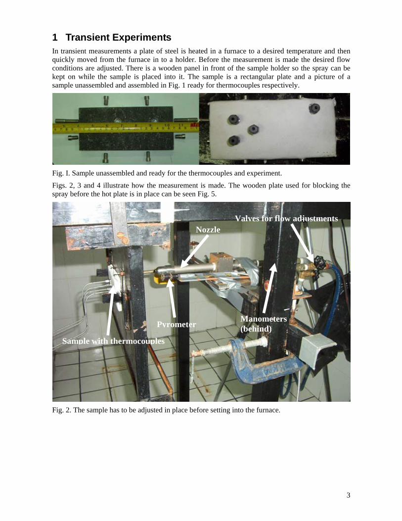
1 Transient Experiments In transient measurements a plate of steel is heated in a furnace to a desired temperature and then quickly moved from the furnace in to a holder. Before the measurement is made the desired flow conditions are adjusted. There is a wooden panel in front of the sample holder so the spray can be kept on while the sample is placed into it. The sample is a rectangular plate and a picture of a sample unassembled and assembled in Fig. 1 ready for thermocouples respectively.

Fig. I. Sample unassembled and ready for the thermocouples and experiment.

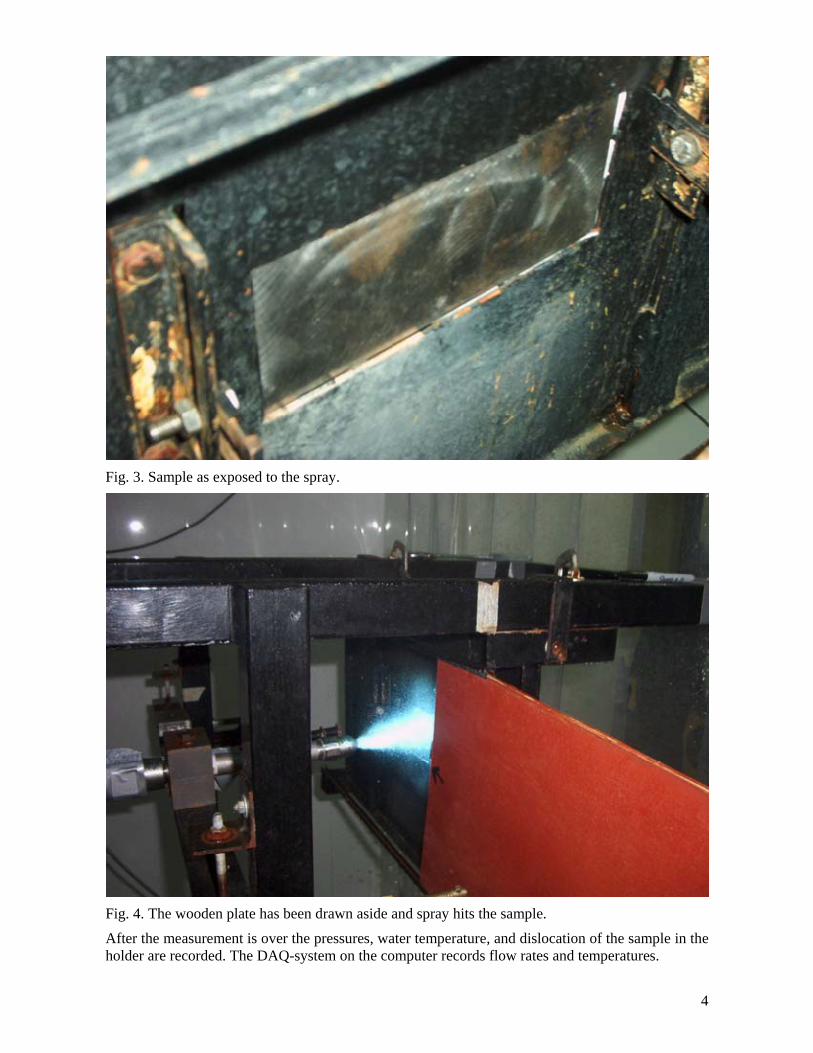
Figs. 2, 3 and 4 illustrate how the measurement is made. The wooden plate used for blocking the spray before the hot plate is in place can be seen Fig. 5.

Fig. 2. The sample has to be adjusted in place before setting into the furnace.

Sample with thermocouples

Pyrometer

NozzleValves for flow adjustments

Manometers (behind)

4

Fig. 3. Sample as exposed to the spray.

Fig. 4. The wooden plate has been drawn aside and spray hits the sample.

After the measurement is over the pressures, water temperature, and dislocation of the sample in the holder are recorded. The DAQ-system on the computer records flow rates and temperatures.

5

1.1 Analysis of The Results The cooling curves measured in the experiments need to be converted into heat flux at the surface and the surface temperature has to be calculated. This is done using an inverse model CONTA. Inverse heat conduction problem (IHCP) is an “ill-posed” problem and does not satisfy general conditions of existence, uniqueness and stability causing a difficulty in defining what the solution is. This means that for every realistic surface flux history, temperatures can be calculated as a function of time at an interior position. Other values arbitrarily close to these calculated temperatures can be produced with an infinite number of surface fluxes. Each of these fluxes would have the same basic heat flux as the original case but there could be high frequency sinusoidal components superimposed upon the basic heat flux. Because of that it is required to restrict the surface flux to having acceptable time variations.

Many methods to solve IHCP have been proposed but most of them can only solve linear cases. The most widely used method to solve nonlinear case is a sequential and involves the use of future temperatures for each calculated component of the surface flux. By sequential is meant estimating one or some small number of components of heat flux at each time step instead of trying to iterate the whole set of heat flux components at once. This procedure permits much smaller time steps than making calculated interior temperatures equal the measured values and allows much more information to be derived about time variation of the surface heat flux than large time steps.

As the time steps are made small, the oscillations tend to have higher amplitudes and frequencies. High frequency in IHCP context means flux components with periods equal or shorter as the time steps between the heat flux components. These high frequencies then need to be filtered out to stabilize the solutions. There are many ways for doing that but in CONTA the function specification method is used meaning the surface heat flux is given a functional form. Function is created using number of constants derived from measured temperatures by least square method.

To increase computational speed of CONTA some simplifications are made that may affect the accuracy of the results.

- The first is assumption of materials properties from previous time step in present and in the selected amount of future time steps. This is done in order to avoid iteration and give the equation a linear form.

- A temporary assumption of constant heat flux over the future time steps used in finding the heat flux of the present time.

In the case of this study with cooling rates over 200°C/s these simplifications has to be taken into account when the time step size is selected. [1]

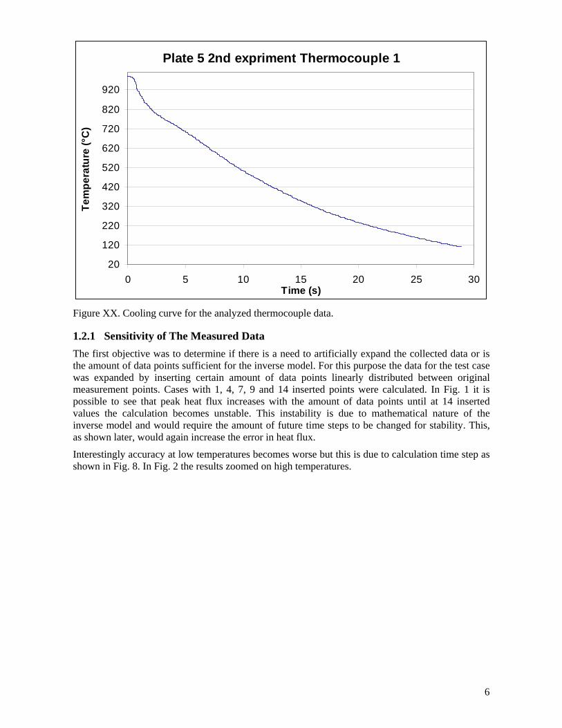
1.2 Sensitivity Analysis of The Inverse Model Plate 5 thermocouple 1 in the second experiment was selected as the test case for this investigation. There are three parameters in the inverse code that need to be investigated: time step between data points, number of future time steps and time step of the calculation.

6

Plate 5 2nd expriment Thermocouple 1

20

120

220

320

420

520

620

720

820

920

0 5 10 15 20 25 30Time (s)

Tem

pera

ture

(°C

)

Figure XX. Cooling curve for the analyzed thermocouple data.

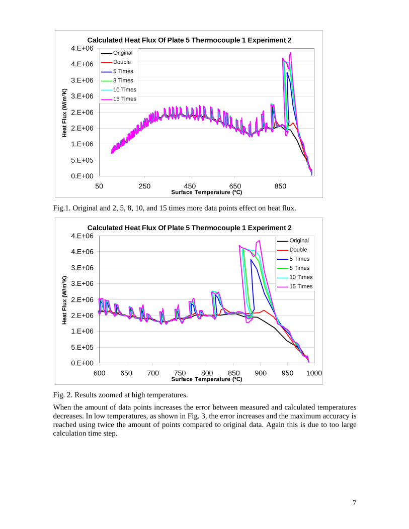
1.2.1 Sensitivity of The Measured Data The first objective was to determine if there is a need to artificially expand the collected data or is the amount of data points sufficient for the inverse model. For this purpose the data for the test case was expanded by inserting certain amount of data points linearly distributed between original measurement points. Cases with 1, 4, 7, 9 and 14 inserted points were calculated. In Fig. 1 it is possible to see that peak heat flux increases with the amount of data points until at 14 inserted values the calculation becomes unstable. This instability is due to mathematical nature of the inverse model and would require the amount of future time steps to be changed for stability. This, as shown later, would again increase the error in heat flux.

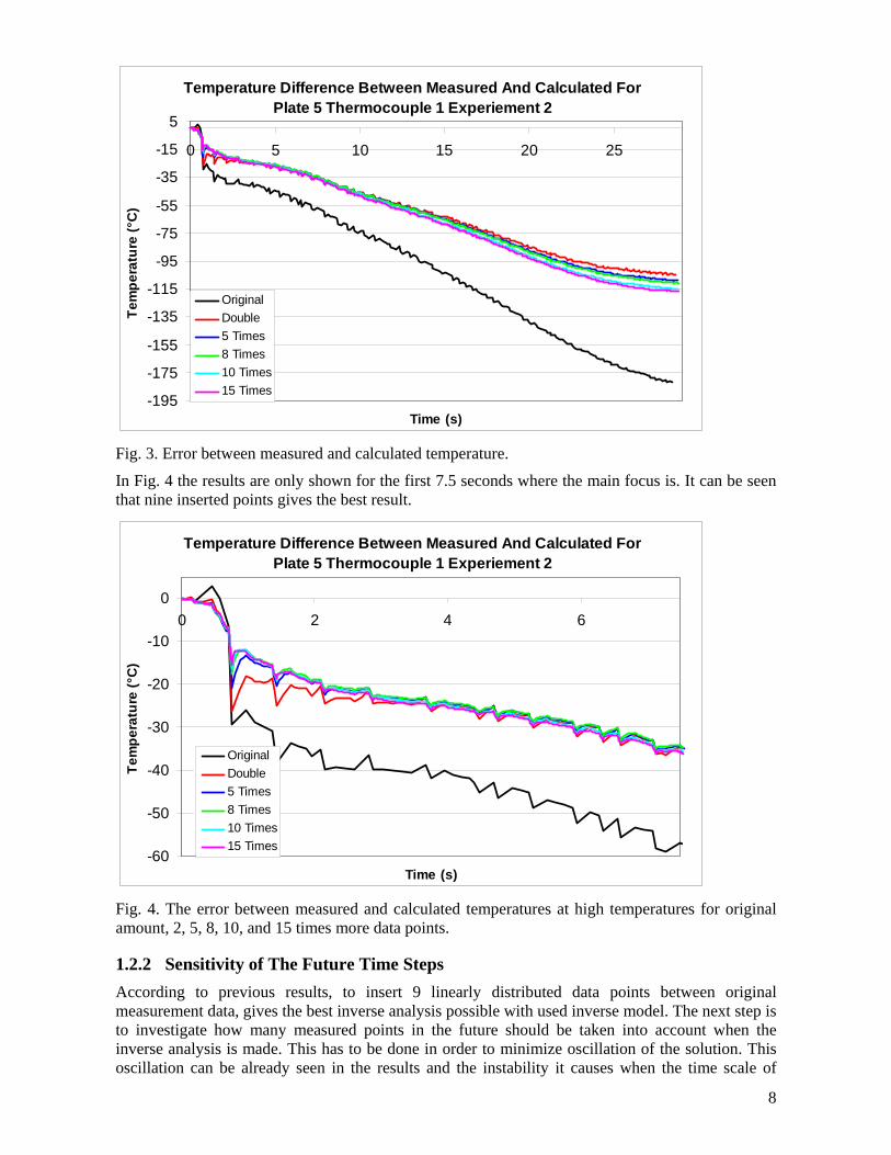
Interestingly accuracy at low temperatures becomes worse but this is due to calculation time step as shown in Fig. 8. In Fig. 2 the results zoomed on high temperatures.

7

Calculated Heat Flux Of Plate 5 Thermocouple 1 Experiment 2

0.E+00

5.E+05

1.E+06

2.E+06

2.E+06

3.E+06

3.E+06

4.E+06

4.E+06

50 250 450 650 850Surface Temperature (°C)

Hea

t Flu

x (W

/m²K

)

OriginalDouble5 Times8 Times10 Times15 Times

Fig.1. Original and 2, 5, 8, 10, and 15 times more data points effect on heat flux.

Calculated Heat Flux Of Plate 5 Thermocouple 1 Experiment 2

0.E+00

5.E+05

1.E+06

2.E+06

2.E+06

3.E+06

3.E+06

4.E+06

4.E+06

600 650 700 750 800 850 900 950 1000Surface Temperature (°C)

Heat

Flu

x (W

/m²K

)

OriginalDouble5 Times8 Times10 Times15 Times

Fig. 2. Results zoomed at high temperatures.

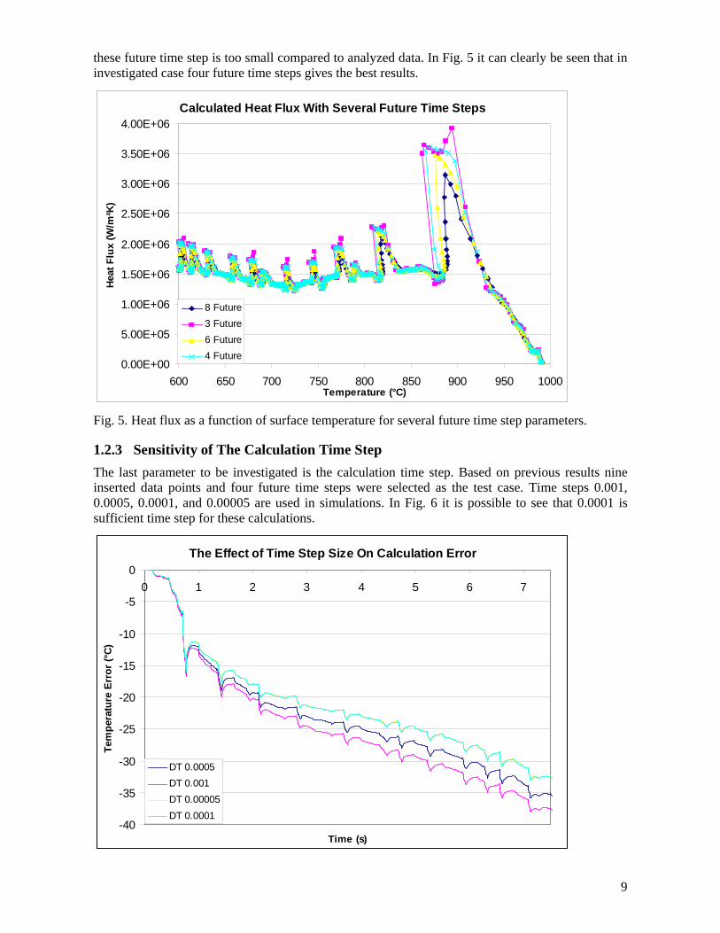
When the amount of data points increases the error between measured and calculated temperatures decreases. In low temperatures, as shown in Fig. 3, the error increases and the maximum accuracy is reached using twice the amount of points compared to original data. Again this is due to too large calculation time step.

8

Temperature Difference Between Measured And Calculated For Plate 5 Thermocouple 1 Experiement 2

-195

-175

-155

-135

-115

-95

-75

-55

-35

-15

5

0 5 10 15 20 25

Time (s)

Tem

pera

ture

(°C

)

OriginalDouble5 Times8 Times10 Times15 Times

Fig. 3. Error between measured and calculated temperature.

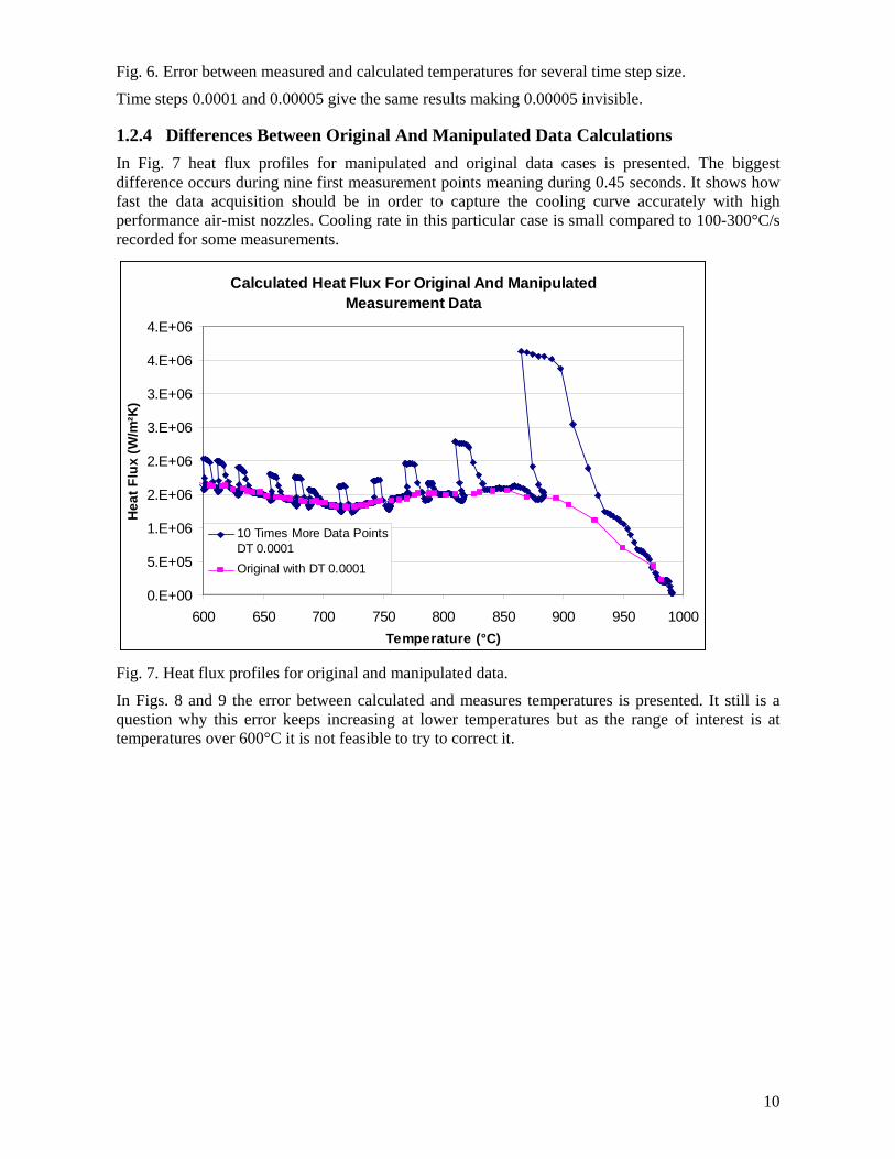
In Fig. 4 the results are only shown for the first 7.5 seconds where the main focus is. It can be seen that nine inserted points gives the best result.

Temperature Difference Between Measured And Calculated For Plate 5 Thermocouple 1 Experiement 2

-60

-50

-40

-30

-20

-10

00 2 4 6

Time (s)

Tem

pera

ture

(°C

)

OriginalDouble5 Times8 Times10 Times15 Times

Fig. 4. The error between measured and calculated temperatures at high temperatures for original amount, 2, 5, 8, 10, and 15 times more data points.

1.2.2 Sensitivity of The Future Time Steps According to previous results, to insert 9 linearly distributed data points between original measurement data, gives the best inverse analysis possible with used inverse model. The next step is to investigate how many measured points in the future should be taken into account when the inverse analysis is made. This has to be done in order to minimize oscillation of the solution. This oscillation can be already seen in the results and the instability it causes when the time scale of

9

these future time step is too small compared to analyzed data. In Fig. 5 it can clearly be seen that in investigated case four future time steps gives the best results.

Calculated Heat Flux With Several Future Time Steps

0.00E+00

5.00E+05

1.00E+06

1.50E+06

2.00E+06

2.50E+06

3.00E+06

3.50E+06

4.00E+06

600 650 700 750 800 850 900 950 1000Temperature (°C)

Hea

t Flu

x (W

/m²K

)

8 Future3 Future6 Future4 Future

Fig. 5. Heat flux as a function of surface temperature for several future time step parameters.

1.2.3 Sensitivity of The Calculation Time Step The last parameter to be investigated is the calculation time step. Based on previous results nine inserted data points and four future time steps were selected as the test case. Time steps 0.001, 0.0005, 0.0001, and 0.00005 are used in simulations. In Fig. 6 it is possible to see that 0.0001 is sufficient time step for these calculations.

The Effect of Time Step Size On Calculation Error

-40

-35

-30

-25

-20

-15

-10

-5

00 1 2 3 4 5 6 7

Time (s)

Tem

pera

ture

Err

or (°

C)

DT 0.0005DT 0.001DT 0.00005DT 0.0001

10

Fig. 6. Error between measured and calculated temperatures for several time step size.

Time steps 0.0001 and 0.00005 give the same results making 0.00005 invisible.

1.2.4 Differences Between Original And Manipulated Data Calculations In Fig. 7 heat flux profiles for manipulated and original data cases is presented. The biggest difference occurs during nine first measurement points meaning during 0.45 seconds. It shows how fast the data acquisition should be in order to capture the cooling curve accurately with high performance air-mist nozzles. Cooling rate in this particular case is small compared to 100-300°C/s recorded for some measurements.

Calculated Heat Flux For Original And Manipulated Measurement Data

0.E+00

5.E+05

1.E+06

2.E+06

2.E+06

3.E+06

3.E+06

4.E+06

4.E+06

600 650 700 750 800 850 900 950 1000Temperature (°C)

Hea

t Flu

x (W

/m²K

)

10 Times More Data PointsDT 0.0001Original with DT 0.0001

Fig. 7. Heat flux profiles for original and manipulated data.

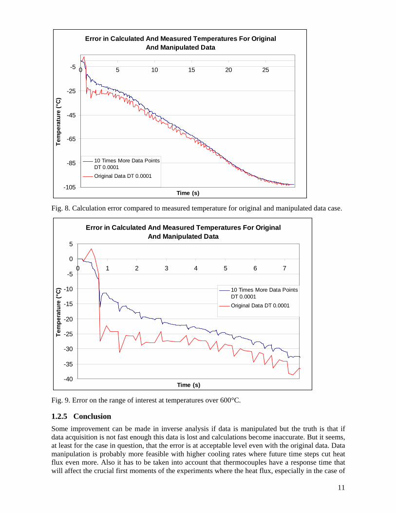
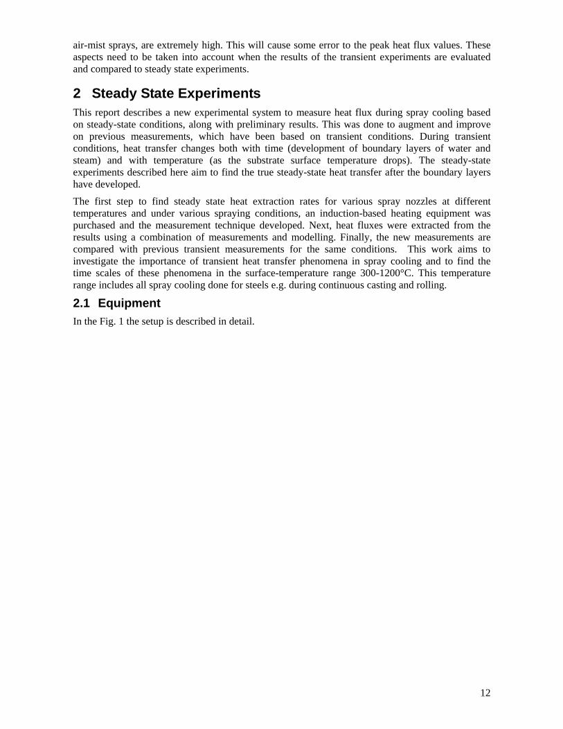
In Figs. 8 and 9 the error between calculated and measures temperatures is presented. It still is a question why this error keeps increasing at lower temperatures but as the range of interest is at temperatures over 600°C it is not feasible to try to correct it.

11

Error in Calculated And Measured Temperatures For Original And Manipulated Data

-105

-85

-65

-45

-25

-5 0 5 10 15 20 25

Time (s)

Tem

pera

ture

(°C

)

10 Times More Data PointsDT 0.0001Original Data DT 0.0001

Fig. 8. Calculation error compared to measured temperature for original and manipulated data case.

Error in Calculated And Measured Temperatures For Original And Manipulated Data

-40

-35

-30

-25

-20

-15

-10

-5

0

5

0 1 2 3 4 5 6 7

Time (s)

Tem

pera

ture

(°C

) 10 Times More Data PointsDT 0.0001Original Data DT 0.0001

Fig. 9. Error on the range of interest at temperatures over 600°C.

1.2.5 Conclusion Some improvement can be made in inverse analysis if data is manipulated but the truth is that if data acquisition is not fast enough this data is lost and calculations become inaccurate. But it seems, at least for the case in question, that the error is at acceptable level even with the original data. Data manipulation is probably more feasible with higher cooling rates where future time steps cut heat flux even more. Also it has to be taken into account that thermocouples have a response time that will affect the crucial first moments of the experiments where the heat flux, especially in the case of

12

air-mist sprays, are extremely high. This will cause some error to the peak heat flux values. These aspects need to be taken into account when the results of the transient experiments are evaluated and compared to steady state experiments.

2 Steady State Experiments This report describes a new experimental system to measure heat flux during spray cooling based on steady-state conditions, along with preliminary results. This was done to augment and improve on previous measurements, which have been based on transient conditions. During transient conditions, heat transfer changes both with time (development of boundary layers of water and steam) and with temperature (as the substrate surface temperature drops). The steady-state experiments described here aim to find the true steady-state heat transfer after the boundary layers have developed.

The first step to find steady state heat extraction rates for various spray nozzles at different temperatures and under various spraying conditions, an induction-based heating equipment was purchased and the measurement technique developed. Next, heat fluxes were extracted from the results using a combination of measurements and modelling. Finally, the new measurements are compared with previous transient measurements for the same conditions. This work aims to investigate the importance of transient heat transfer phenomena in spray cooling and to find the time scales of these phenomena in the surface-temperature range 300-1200°C. This temperature range includes all spray cooling done for steels e.g. during continuous casting and rolling.

2.1 Equipment In the Fig. 1 the setup is described in detail.

13

Figure 1. Steady state spray cooling apparatus.

Using National Instruments SCXI-1000 box together with two SCXI-1302 terminals several signals are collected from the measurement system: sample temperature from the controller, total power taken by the power supply, cooling water temperature raise between the cooling unit and power supply, two surface temperatures from the ceramic and spray properties including pressure and flow rates for both air and water. Acquisition sampling time is 0.05 seconds. All cables are shielded either by manufacturer using a braid and that has been grounded or simply applying aluminium foil around the cables as done in the case of thermocouples. The nominal maximum power the power supply can deliver is 5000W but it can be loaded up to 110% of the nominal making the maximum to be 5500W. Thermocouples used are of K-type. Currently also water temperature measurements are made using exposed tip K-type thermocouples. Samples used are AISI-304L stainless steel that is paramagnetic in order to avoid problems caused by the Curie-temperature and to minimize oxidation. The materials properties of the ceramic, steel and copper are given in the Appendix A.

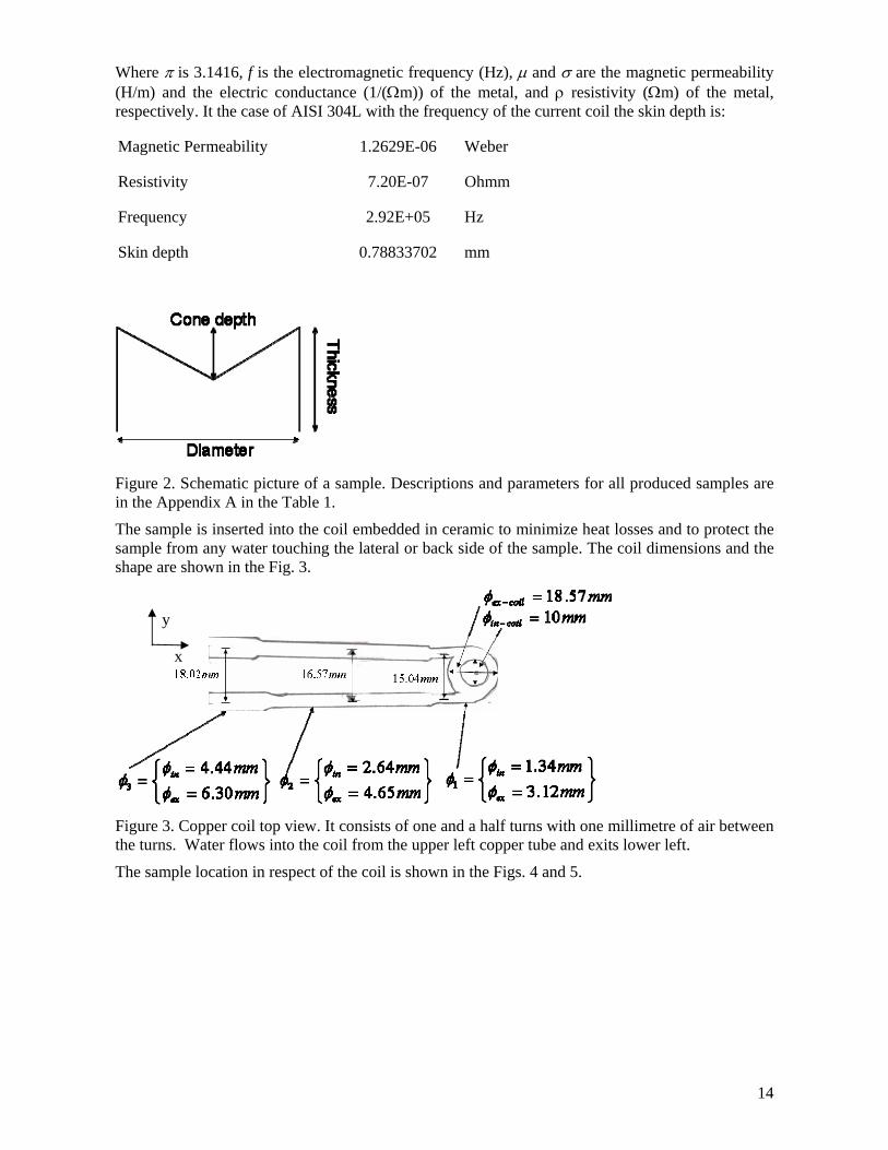
A schematic shape of the sample is shown in the Fig. 2. The thermocouple used for controlling the temperature in the sample is welded in the centre, the closest place to the sprayed surface and the heating is applied on the periphery of the sample where induction currents circle the sample surface within the skin depth. The skin depth, δ, is the thickness of the superficial layer where the induced current is practically confined and it is defined using Eq. 1.

σπρ

μσπδ

ff==

1 (1)

14

Where π is 3.1416, f is the electromagnetic frequency (Hz), μ and σ are the magnetic permeability (H/m) and the electric conductance (1/(Ωm)) of the metal, and ρ resistivity (Ωm) of the metal, respectively. It the case of AISI 304L with the frequency of the current coil the skin depth is:

Magnetic Permeability 1.2629E-06 Weber

Resistivity 7.20E-07 Ohmm

Frequency 2.92E+05 Hz

Skin depth 0.78833702 mm

Figure 2. Schematic picture of a sample. Descriptions and parameters for all produced samples are in the Appendix A in the Table 1.

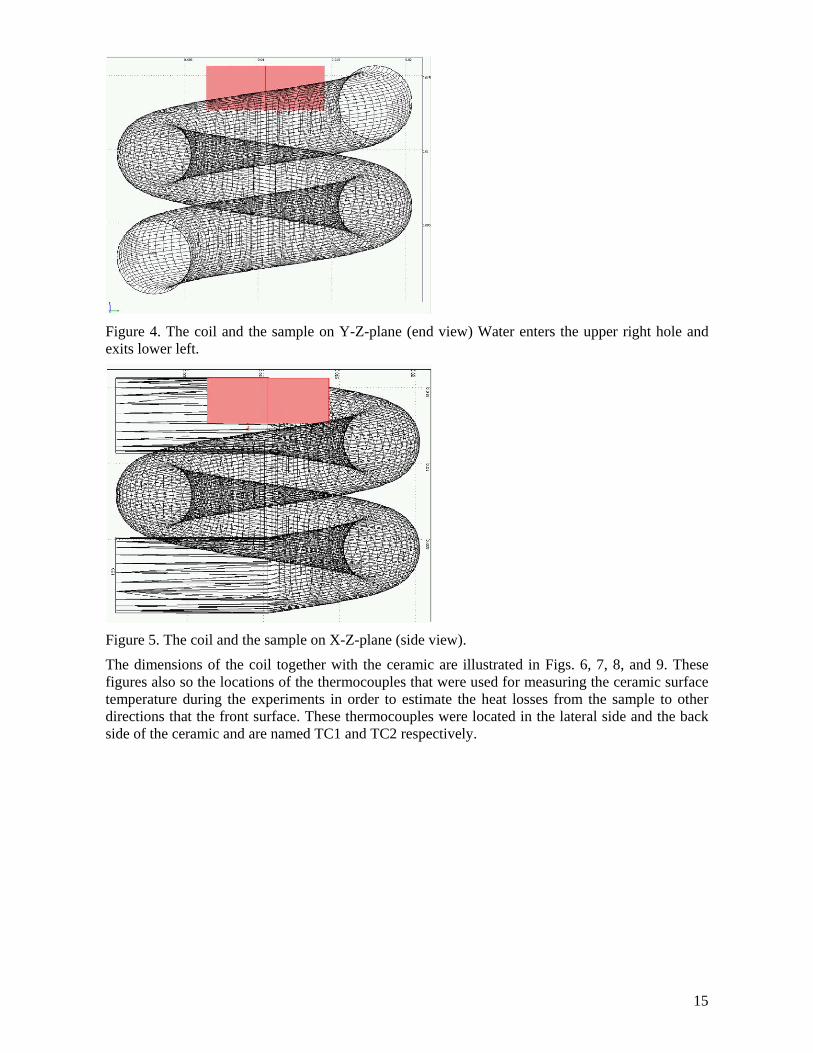
The sample is inserted into the coil embedded in ceramic to minimize heat losses and to protect the sample from any water touching the lateral or back side of the sample. The coil dimensions and the shape are shown in the Fig. 3.

Figure 3. Copper coil top view. It consists of one and a half turns with one millimetre of air between the turns. Water flows into the coil from the upper left copper tube and exits lower left.

The sample location in respect of the coil is shown in the Figs. 4 and 5.

x

y

15

Figure 4. The coil and the sample on Y-Z-plane (end view) Water enters the upper right hole and exits lower left.

Figure 5. The coil and the sample on X-Z-plane (side view).

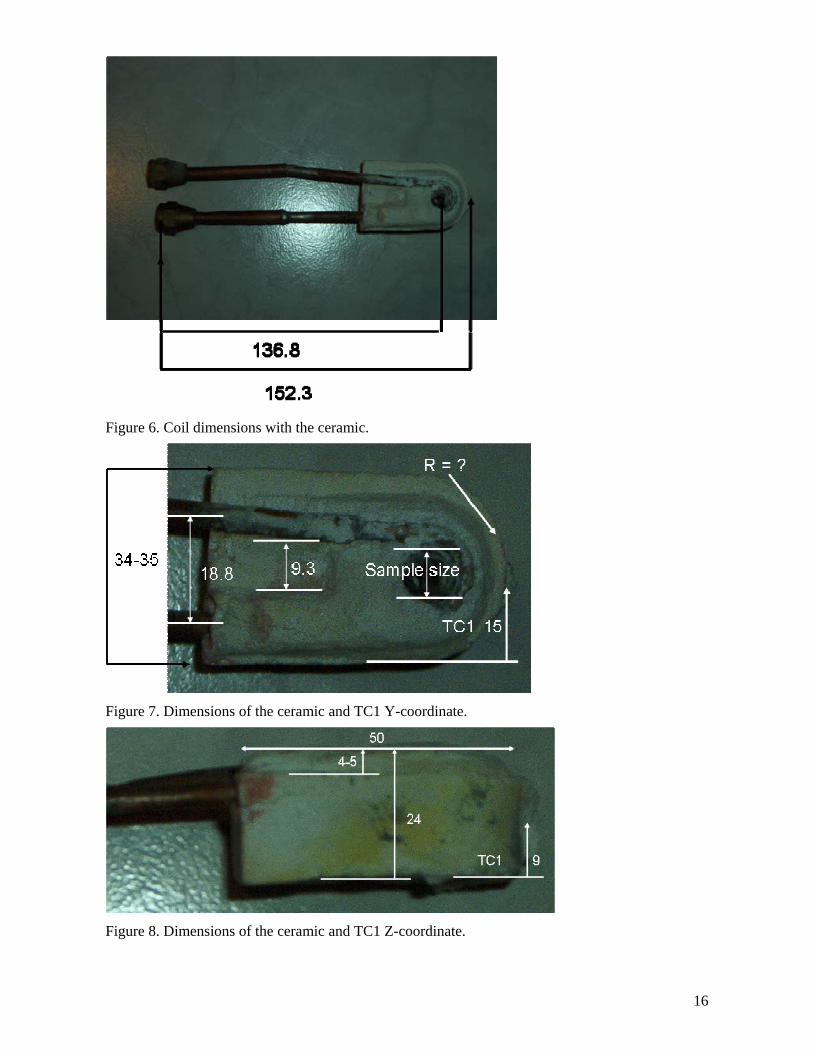
The dimensions of the coil together with the ceramic are illustrated in Figs. 6, 7, 8, and 9. These figures also so the locations of the thermocouples that were used for measuring the ceramic surface temperature during the experiments in order to estimate the heat losses from the sample to other directions that the front surface. These thermocouples were located in the lateral side and the back side of the ceramic and are named TC1 and TC2 respectively.

16

Figure 6. Coil dimensions with the ceramic.

Figure 7. Dimensions of the ceramic and TC1 Y-coordinate.

Figure 8. Dimensions of the ceramic and TC1 Z-coordinate.

17

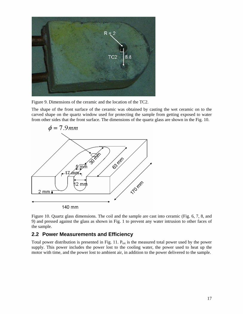
Figure 9. Dimensions of the ceramic and the location of the TC2.

The shape of the front surface of the ceramic was obtained by casting the wet ceramic on to the carved shape on the quartz window used for protecting the sample from getting exposed to water from other sides that the front surface. The dimensions of the quartz glass are shown in the Fig. 10.

Figure 10. Quartz glass dimensions. The coil and the sample are cast into ceramic (Fig. 6, 7, 8, and 9) and pressed against the glass as shown in Fig. 1 to prevent any water intrusion to other faces of the sample.

2.2 Power Measurements and Efficiency Total power distribution is presented in Fig. 11. Ptot is the measured total power used by the power supply. This power includes the power lost to the cooling water, the power used to heat up the motor with time, and the power lost to ambient air, in addition to the power delivered to the sample.

18

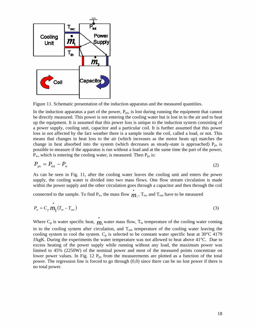
Figure 11. Schematic presentation of the induction apparatus and the measured quantities.

In the induction apparatus a part of the power, Pps, is lost during running the equipment that cannot be directly measured. This power is not entering the cooling water but is lost in to the air and to heat up the equipment. It is assumed that this power loss is unique to the induction system consisting of a power supply, cooling unit, capacitor and a particular coil. It is further assumed that this power loss in not affected by the fact weather there is a sample inside the coil, called a load, or not. This means that changes in heat loss to the air (which increases as the motor heats up) matches the change in heat absorbed into the system (which decreases as steady-state is approached) Pps is possible to measure if the apparatus is run without a load and at the same time the part of the power, Pw, which is entering the cooling water, is measured. Then Pps is:

wtotps PPP −= (2)

As can be seen in Fig. 11, after the cooling water leaves the cooling unit and enters the power supply, the cooling water is divided into two mass flows. One flow stream circulation is made within the power supply and the other circulation goes through a capacitor and then through the coil

connected to the sample. To find Pw, the mass flow 1m

•

, Tin, and Tout have to be measured

( )outinpw TTCP m −=•

1 (3)

Where Cp is water specific heat, 1m•

water mass flow, Tin temperature of the cooling water coming in to the cooling system after circulation, and Tout temperature of the cooling water leaving the cooling system to cool the system. Cp is selected to be constant water specific heat at 30°C 4179 J/kgK. During the experiments the water temperature was not allowed to heat above 41°C. Due to excess heating of the power supply while running without any load, the maximum power was limited to 45% (2250W) of the nominal power and most of the measured points concentrate on lower power values. In Fig. 12 Pps from the measurements are plotted as a function of the total power. The regression line is forced to go through (0,0) since there can be no lost power if there is no total power.

19

Pps Measurements

y = 0.3013xR2 = 0.9516

0

100

200

300

400

500

600

700

800

900

0 500 1000 1500 2000 2500 3000Total Power (W)

Pps

(W)

PpsLinear (Pps)

Figure 12. Measured Pps as a function of the total power.

It was found out that Pps is a linear function of the total power with some uncertainty.

(1 )ps ps totP Pη= − × , (4a)

The power supply efficiency, ηps, is seen to be ~70%, based on the slope of 0.3013 in the figure.

The known Y-error is caused by inaccuracy of the total power and cooling water measurements (±35W and ±20W respectively) and X-error caused by inaccuracy in total power measurement. The experiments using the samples were made with the measurement setup corresponding to the Pps measurement in the Fig. 12. The total power of all measurements were multiplied with a coefficient named Potencia actual derived from the Fig. 12. Actual power can be calculated using Eq. 4b.

A ps totP Pη= × (4b)

Where PA is the measurable power used for heating the sample and cooling water of the whole induction apparatus, Ptot the total measured power from the power supply.

As the high level of scattering was noticed the cabling was altered in order to lower the amount of the scattering. In Fig.13 the Pps measurements for the new cabling are shown and noticeable change in the slope can be seen. As can be seen the scattering is greater than error caused by known measurement errors in both cases. Causes for the error can be behaviour of the equipment changes when water cooling unit is on or the power supply’s internal temperature change. The known measurement errors are caused by noise in the measurement system. Noise in total power measurement has now been decreased to ±1.5W. Noise in cooling water power still remains the same and we expect some improvement by replacing the thermocouples and possibly rewiring.

20

Pps Using New Cabling

y = 0.2038xR2 = 0.9202

0

100

200

300

400

500

600

0 500 1000 1500 2000 2500 3000

Total Power (W)

Pps

(W)

Pps New ConfigurationLinear (Pps New Configuration)

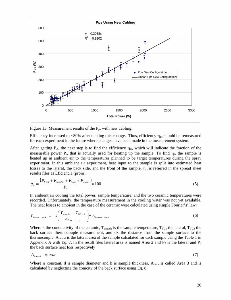
Figure 13. Measurement results of the Pps with new cabling.

Efficiency increased to ~80% after making this change. Thus, efficiency ηps should be remeasured for each experiment in the future where changes have been made in the measurement system.

After getting PA, the next step is to find the efficiency ηis, which will indicate the fraction of the measurable power PA that is actually used for heating up the sample. To find ηis the sample is heated up in ambient air to the temperatures planned to be target temperatures during the spray experiment. In this ambient air experiment, heat input to the sample is split into estimated heat losses to the lateral, the back side, and the front of the sample. ηis is referred in the spread sheet results files as Eficiencia (prom).

( )100×

+++=

A

lateralbackannularfrontis P

PPPPη (5)

In ambient air cooling the total power, sample temperature, and the two ceramic temperatures were recorded. Unfortunately, the temperature measurement in the cooling water was not yet available. The heat losses to ambient in the case of the ceramic were calculated using simple Fourier’s’ law:

backLateralTCTC

TCsamplebacklateral A

dxTT

kP ,2,1

2,1, *⎟

⎟⎠

⎞⎜⎜⎝

⎛ −−= (6)

Where k the conductivity of the ceramic, Tsample is the sample temperature, TTC1 the lateral, TTC2 the back surface thermocouple measurement, and dx the distance from the sample surface to the thermocouple. Alateral is the lateral area of the sample calculated for each sample using the Table 1 in Appendix A with Eq. 7. In the result files lateral area is named Area 2 and P2 is the lateral and P3 the back surface heat loss respectively

dhAlateral π= (7)

Where π constant, d is sample diameter and h is sample thickness. Aback is called Area 3 and is calculated by neglecting the conicity of the back surface using Eq. 8:

21

4

2dAbackπ

= (8)

The lateral thermocouple (TC1) distance dxTC1 is shown in the analyzed excel files under name distancia p2. It includes an assumption that the distance shown in Figs. 7 and 8 can be neglected because the coil acts as a cooling channel between the thermocouple and the sample. The actual distance dxTC1 is then the distance from the sample surface to the surface of the coil and the thermocouple reading is assumed to be valid at that location. The back face thermocouple (TC2) distance dxTC2 has been treated as is given in the Figs. 8 and 9 and is shown in the files under name distancia p3.

The heat loss through the front surface is calculated using radiation as shown in Eq. 9:

( ) annularfrontambsampleannularfront ATTP ,44

, ×−= σε (9)

Where σ is Stefan-Boltzmann constant, ε is the emissivity of steel, Tsample sample temperature and Tamb the ambient temperature. In the result files Pcont is referred as P1, Afront as A1a, Aannular as A1b, and Tamb as Ta. Afront can be calculated from Eq. 10 and Aannular from Eq. 11 using constants Diametro a and sample diameter. These are illustrated better in the Fig.14.

Figure 14. Schematic presentation of the sample attached to the quartz glass.

( )4

2DiameterAfrontπ

= (10)

( )( )22

4DiameterdAannular −=

π (11)

Where Diametro a is given in the results file and sample diameter d in the Appendix A Table 1. Temperatures are averages over the time the sample was kept on a target temperature, usually 20 seconds.

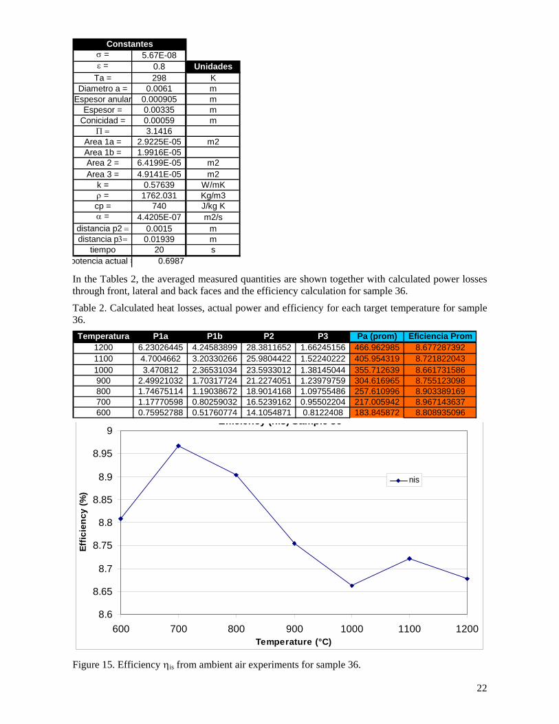
2.3 Results Depending on how well the sample is conserved during the experiments without melting or strong oxidation, only one or two thermal cycle experiments can be made when using a stainless steel sample. In this case sample 36 was used. First the ambient air cooling experiment was conducted in order to find out the efficiency of the induction heating. In Table 1 the necessary constants to conduct calculations mentioned in the chapter 1.2 are shown.

Table 1. Constants for calculating the efficiencies for sample 36.

22

σ = 5.67E-08ε = 0.8 Unidades

Ta = 298 KDiametro a = 0.0061 m

Espesor anular 0.000905 mEspesor = 0.00335 m

Conicidad = 0.00059 mΠ = 3.1416

Area 1a = 2.9225E-05 m2Area 1b = 1.9916E-05Area 2 = 6.4199E-05 m2Area 3 = 4.9141E-05 m2

k = 0.57639 W/mKρ = 1762.031 Kg/m3cp = 740 J/kg Kα = 4.4205E-07 m2/s

distancia p2 = 0.0015 mdistancia p3= 0.01939 m

tiempo 20 spotencia actual = 0.6987

Constantes

In the Tables 2, the averaged measured quantities are shown together with calculated power losses through front, lateral and back faces and the efficiency calculation for sample 36.

Table 2. Calculated heat losses, actual power and efficiency for each target temperature for sample 36.

Temperatura P1a P1b P2 P3 Pa (prom) Eficiencia Prom1200 6.23026445 4.24583899 28.3811652 1.66245156 466.962985 8.6772873921100 4.7004662 3.20330266 25.9804422 1.52240222 405.954319 8.7218220431000 3.470812 2.36531034 23.5933012 1.38145044 355.712639 8.661731586900 2.49921032 1.70317724 21.2274051 1.23979759 304.616965 8.755123098800 1.74675114 1.19038672 18.9014168 1.09755486 257.610996 8.903389169700 1.17770598 0.80259032 16.5239162 0.95502204 217.005942 8.967143637600 0.75952788 0.51760774 14.1054871 0.8122408 183.845872 8.808935096 Efficiency (nis) Sample 36

8.6

8.65

8.7

8.75

8.8

8.85

8.9

8.95

9

600 700 800 900 1000 1100 1200Temperature (°C)

Effic

ienc

y (%

)

nis

Figure 15. Efficiency ηis from ambient air experiments for sample 36.

23

As can be seen the efficiency does not change much over the temperature range indicating that sample properties do not change much over this temperature range.

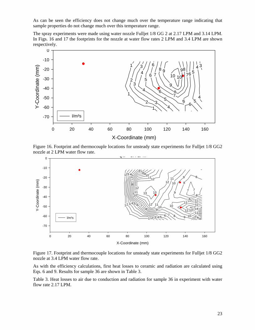
The spray experiments were made using water nozzle Fulljet 1/8 GG 2 at 2.17 LPM and 3.14 LPM. In Figs. 16 and 17 the footprints for the nozzle at water flow rates 2 LPM and 3.4 LPM are shown respectively.

5

5

4

4

3

6

5

5

6

6

6

109

9

8

8

87

7

710

4

43

3

9

2

2

1

1

1

6

643

X-Coordinate (mm)

0 20 40 60 80 100 120 140 160

Y-C

oord

inat

e (m

m)

-70

-60

-50

-40

-30

-20

-10

0

l/m²s

Figure 16. Footprint and thermocouple locations for unsteady state experiments for Fulljet 1/8 GG2 nozzle at 2 LPM water flow rate.

Qw 3.4 LPM

15141312

11

1110

9

9

9 87654

14131211109

8

8

8

77

8

8

8

9

11

11

11

10

10

10

10

9

7

7

7

6

6

6

5

5

5

12

12

4

4

4

3

3

3

2

2

2

1

1

1

13

1211109

13

876

12

X-Coordinate (mm)

0 20 40 60 80 100 120 140 160

Y-C

oord

inat

e (m

m)

-70

-60

-50

-40

-30

-20

-10

0

l/m²s

Figure 17. Footprint and thermocouple locations for unsteady state experiments for Fulljet 1/8 GG2 nozzle at 3.4 LPM water flow rate.

As with the efficiency calculations, first heat losses to ceramic and radiation are calculated using Eqs. 6 and 9. Results for sample 36 are shown in Table 3.

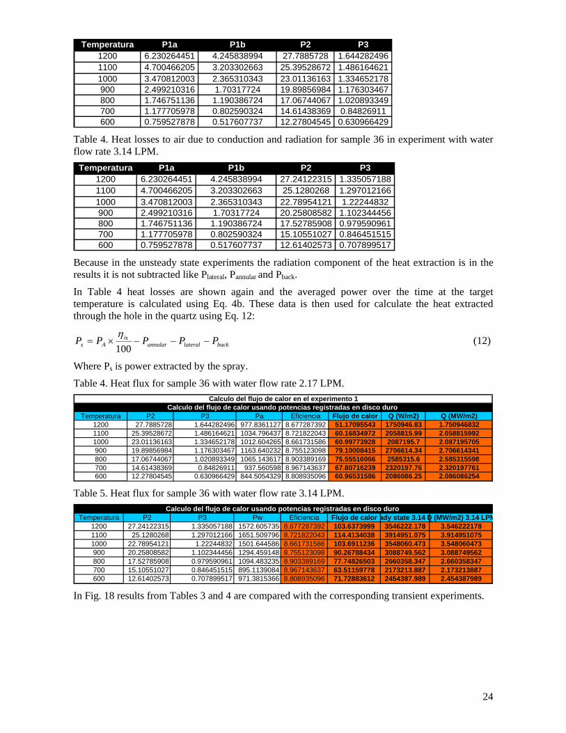
Table 3. Heat losses to air due to conduction and radiation for sample 36 in experiment with water flow rate 2.17 LPM.

24

Temperatura P1a P1b P2 P31200 6.230264451 4.245838994 27.7885728 1.6442824961100 4.700466205 3.203302663 25.39528672 1.4861646211000 3.470812003 2.365310343 23.01136163 1.334652178900 2.499210316 1.70317724 19.89856984 1.176303467800 1.746751136 1.190386724 17.06744067 1.020893349700 1.177705978 0.802590324 14.61438369 0.84826911600 0.759527878 0.517607737 12.27804545 0.630966429

Table 4. Heat losses to air due to conduction and radiation for sample 36 in experiment with water flow rate 3.14 LPM.

Temperatura P1a P1b P2 P31200 6.230264451 4.245838994 27.24122315 1.3350571881100 4.700466205 3.203302663 25.1280268 1.2970121661000 3.470812003 2.365310343 22.78954121 1.22244832900 2.499210316 1.70317724 20.25808582 1.102344456800 1.746751136 1.190386724 17.52785908 0.979590961700 1.177705978 0.802590324 15.10551027 0.846451515600 0.759527878 0.517607737 12.61402573 0.707899517

Because in the unsteady state experiments the radiation component of the heat extraction is in the results it is not subtracted like Plateral, Pannular and Pback.

In Table 4 heat losses are shown again and the averaged power over the time at the target temperature is calculated using Eq. 4b. These data is then used for calculate the heat extracted through the hole in the quartz using Eq. 12:

backlateralannularis

As PPPPP −−−×=100η

(12)

Where Ps is power extracted by the spray.

Table 4. Heat flux for sample 36 with water flow rate 2.17 LPM.

Temperatura P2 P3 Pa Eficiencia Flujo de calor Q (W/m2) Q (MW/m2)1200 27.7885728 1.644282496 977.8361127 8.677287392 51.17095543 1750946.83 1.7509468321100 25.39528672 1.486164621 1034.796437 8.721822043 60.16834972 2058815.99 2.0588159921000 23.01136163 1.334652178 1012.604265 8.661731586 60.99773928 2087195.7 2.087195705900 19.89856984 1.176303467 1163.640232 8.755123098 79.10008415 2706614.34 2.706614341800 17.06744067 1.020893349 1065.143617 8.903389169 75.55516066 2585315.6 2.585315598700 14.61438369 0.84826911 937.560598 8.967143637 67.80716239 2320197.76 2.320197761600 12.27804545 0.630966429 844.5054329 8.808935096 60.96531586 2086086.25 2.086086254

Calculo del flujo de calor en el experimento 1Calculo del flujo de calor usando potencias registradas en disco duro

Table 5. Heat flux for sample 36 with water flow rate 3.14 LPM.

Temperatura P2 P3 Pw Eficiencia Flujo de calor ady state 3.14 LQ (MW/m2) 3.14 LPM1200 27.24122315 1.335057188 1572.605735 8.677287392 103.6373999 3546222.178 3.5462221781100 25.1280268 1.297012166 1651.509796 8.721822043 114.4134038 3914951.075 3.9149510751000 22.78954121 1.22244832 1501.644586 8.661731586 103.6911236 3548060.473 3.548060473900 20.25808582 1.102344456 1294.459148 8.755123098 90.26788434 3088749.562 3.088749562800 17.52785908 0.979590961 1094.483235 8.903389169 77.74826503 2660358.347 2.660358347700 15.10551027 0.846451515 895.1139084 8.967143637 63.51159778 2173213.887 2.173213887600 12.61402573 0.707899517 971.3815366 8.808935096 71.72883612 2454387.989 2.454387989

Calculo del flujo de calor usando potencias registradas en disco duro

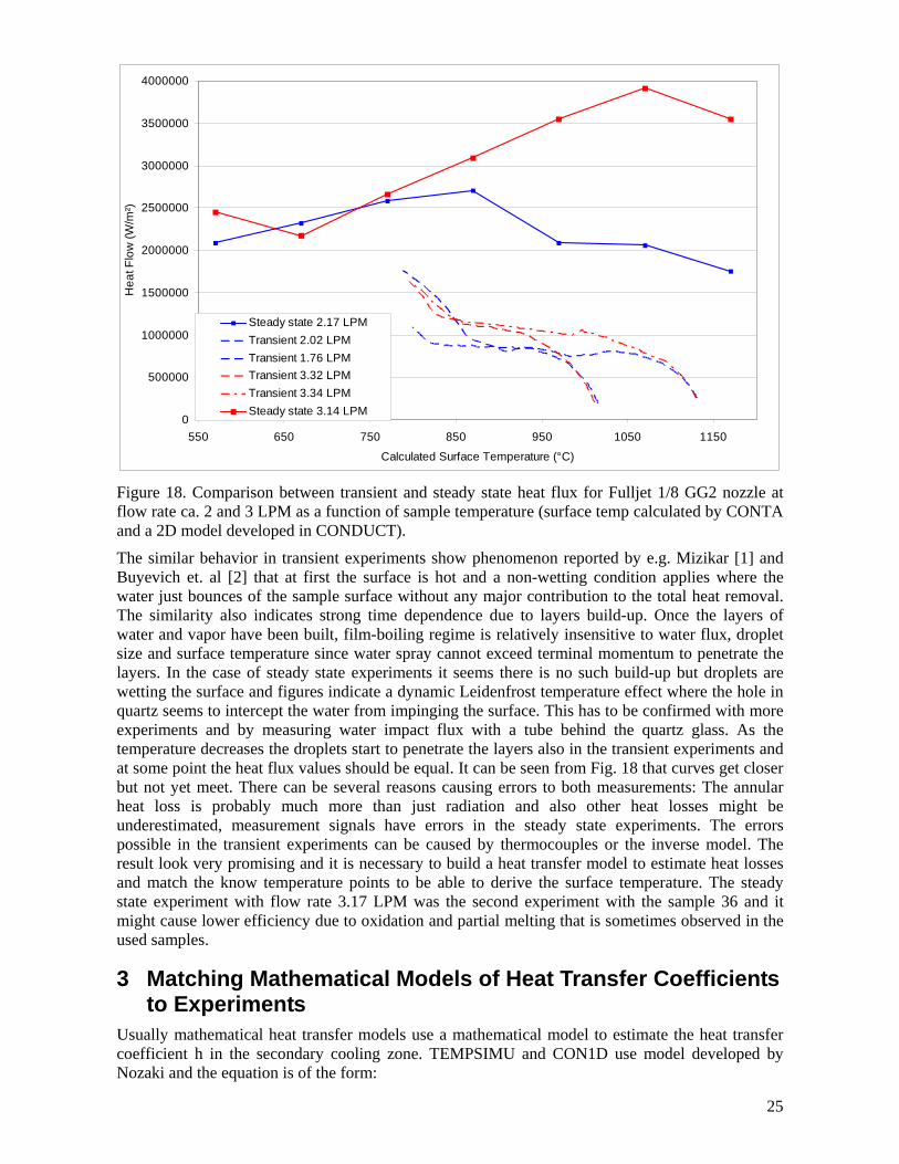
In Fig. 18 results from Tables 3 and 4 are compared with the corresponding transient experiments.

25

0

500000

1000000

1500000

2000000

2500000

3000000

3500000

4000000

550 650 750 850 950 1050 1150

Calculated Surface Temperature (°C)

Hea

t Flo

w (W

/m²)

Steady state 2.17 LPMTransient 2.02 LPMTransient 1.76 LPMTransient 3.32 LPMTransient 3.34 LPMSteady state 3.14 LPM

Figure 18. Comparison between transient and steady state heat flux for Fulljet 1/8 GG2 nozzle at flow rate ca. 2 and 3 LPM as a function of sample temperature (surface temp calculated by CONTA and a 2D model developed in CONDUCT).

The similar behavior in transient experiments show phenomenon reported by e.g. Mizikar [1] and Buyevich et. al [2] that at first the surface is hot and a non-wetting condition applies where the water just bounces of the sample surface without any major contribution to the total heat removal. The similarity also indicates strong time dependence due to layers build-up. Once the layers of water and vapor have been built, film-boiling regime is relatively insensitive to water flux, droplet size and surface temperature since water spray cannot exceed terminal momentum to penetrate the layers. In the case of steady state experiments it seems there is no such build-up but droplets are wetting the surface and figures indicate a dynamic Leidenfrost temperature effect where the hole in quartz seems to intercept the water from impinging the surface. This has to be confirmed with more experiments and by measuring water impact flux with a tube behind the quartz glass. As the temperature decreases the droplets start to penetrate the layers also in the transient experiments and at some point the heat flux values should be equal. It can be seen from Fig. 18 that curves get closer but not yet meet. There can be several reasons causing errors to both measurements: The annular heat loss is probably much more than just radiation and also other heat losses might be underestimated, measurement signals have errors in the steady state experiments. The errors possible in the transient experiments can be caused by thermocouples or the inverse model. The result look very promising and it is necessary to build a heat transfer model to estimate heat losses and match the know temperature points to be able to derive the surface temperature. The steady state experiment with flow rate 3.17 LPM was the second experiment with the sample 36 and it might cause lower efficiency due to oxidation and partial melting that is sometimes observed in the used samples.

3 Matching Mathematical Models of Heat Transfer Coefficients to Experiments

Usually mathematical heat transfer models use a mathematical model to estimate the heat transfer coefficient h in the secondary cooling zone. TEMPSIMU and CON1D use model developed by Nozaki and the equation is of the form:

26

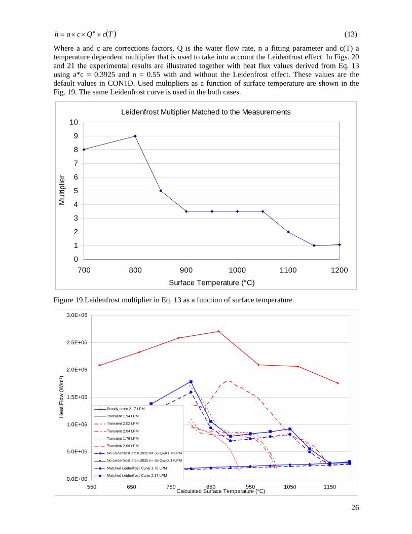
( )TcQcah n ×××= (13)

Where a and c are corrections factors, Q is the water flow rate, n a fitting parameter and c(T) a temperature dependent multiplier that is used to take into account the Leidenfrost effect. In Figs. 20 and 21 the experimental results are illustrated together with heat flux values derived from Eq. 13 using a*c = 0.3925 and n = 0.55 with and without the Leidenfrost effect. These values are the default values in CON1D. Used multipliers as a function of surface temperature are shown in the Fig. 19. The same Leidenfrost curve is used in the both cases.

Leidenfrost Multiplier Matched to the Measurements

0

1

2

3

4

5

6

7

8

9

10

700 800 900 1000 1100 1200

Surface Temperature (°C)

Mul

tiplie

r

Figure 19.Leidenfrost multiplier in Eq. 13 as a function of surface temperature.

0.0E+00

5.0E+05

1.0E+06

1.5E+06

2.0E+06

2.5E+06

3.0E+06

550 650 750 850 950 1050 1150Calculated Surface Temperature (°C)

Hea

t Flo

w (W

/m²)

Steady state 2.17 LPM

Transient 1.94 LPM

Transient 2.02 LPM

Transient 2.04 LPM

Transient 1.76 LPM

Transient 2.09 LPM

No Leidenfrost a*c=.3925 n=.55 Qw=1.76LPM

No Leidenfrost a*c=.3925 n=.55 Qw=2.17LPM

Matched Leidenfrost Curve 1.76 LPM

Matched Leidenfrost Curve 2.17 LPM

27

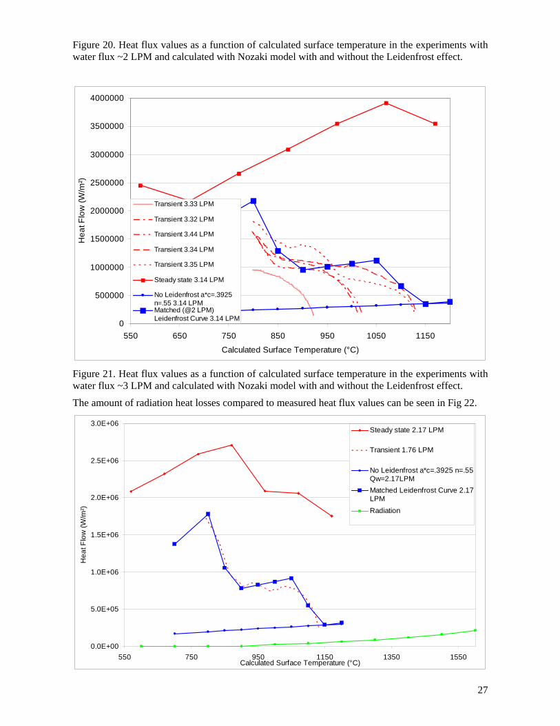
Figure 20. Heat flux values as a function of calculated surface temperature in the experiments with water flux ~2 LPM and calculated with Nozaki model with and without the Leidenfrost effect.

0

500000

1000000

1500000

2000000

2500000

3000000

3500000

4000000

550 650 750 850 950 1050 1150

Calculated Surface Temperature (°C)

Hea

t Flo

w (W

/m²)

Transient 3.33 LPM

Transient 3.32 LPM

Transient 3.44 LPM

Transient 3.34 LPM

Transient 3.35 LPM

Steady state 3.14 LPM

No Leidenfrost a*c=.3925n=.55 3.14 LPMMatched (@2 LPM) Leidenfrost Curve 3.14 LPM

Figure 21. Heat flux values as a function of calculated surface temperature in the experiments with water flux ~3 LPM and calculated with Nozaki model with and without the Leidenfrost effect.

The amount of radiation heat losses compared to measured heat flux values can be seen in Fig 22.

0.0E+00

5.0E+05

1.0E+06

1.5E+06

2.0E+06

2.5E+06

3.0E+06

550 750 950 1150 1350 1550Calculated Surface Temperature (°C)

Hea

t Flo

w (W

/m²)

Steady state 2.17 LPM

Transient 1.76 LPM

No Leidenfrost a*c=.3925 n=.55Qw=2.17LPMMatched Leidenfrost Curve 2.17LPMRadiation

28

FUTURE WORK:

- Figures, tables and equations are not numbered

- Industrial validation

- Temperature vs. time for both transient and steady state measurements

- sensitivity analysis also for transient water spray

- Make conduct model to match our cases and develop the COMSOL model in 3D

- Conclusions

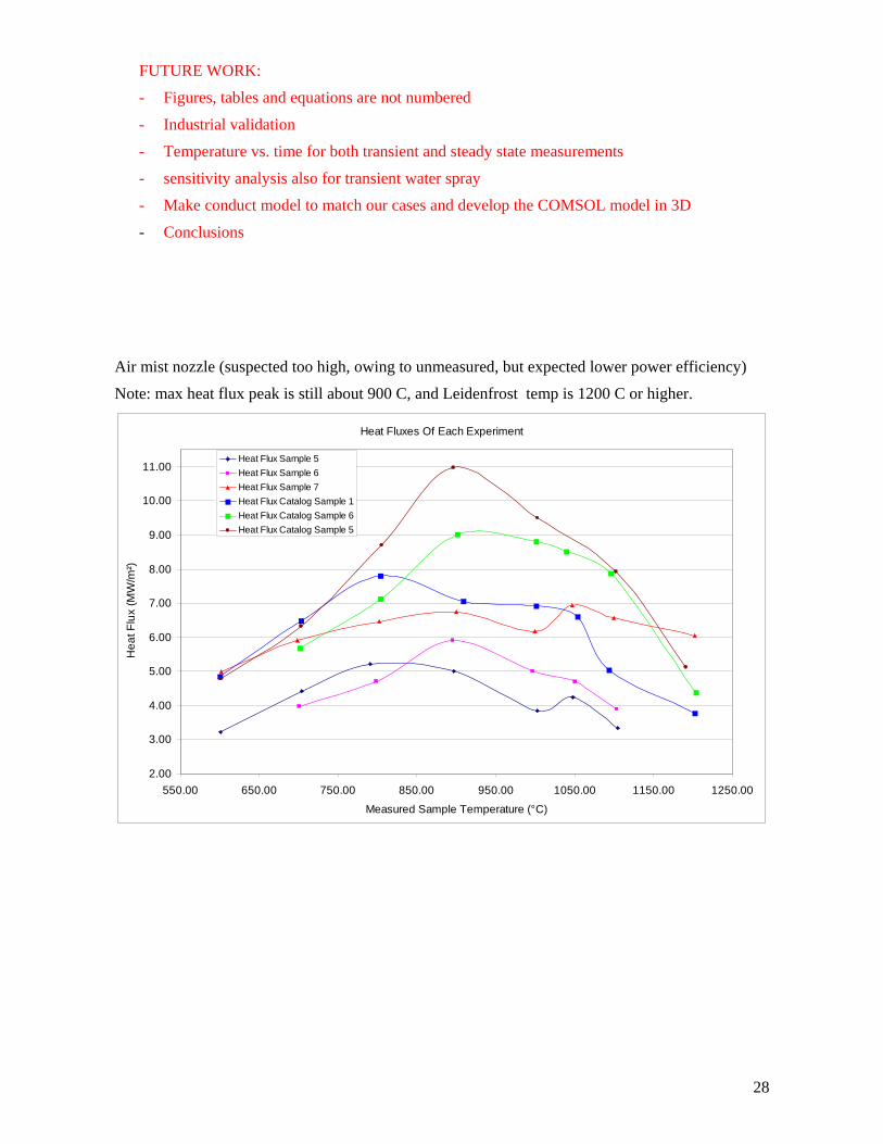
Air mist nozzle (suspected too high, owing to unmeasured, but expected lower power efficiency)

Note: max heat flux peak is still about 900 C, and Leidenfrost temp is 1200 C or higher.

Heat Fluxes Of Each Experiment

2.00

3.00

4.00

5.00

6.00

7.00

8.00

9.00

10.00

11.00

550.00 650.00 750.00 850.00 950.00 1050.00 1150.00 1250.00

Measured Sample Temperature (°C)

Hea

t Flu

x (M

W/m

²)

Heat Flux Sample 5Heat Flux Sample 6Heat Flux Sample 7Heat Flux Catalog Sample 1Heat Flux Catalog Sample 6Heat Flux Catalog Sample 5

29

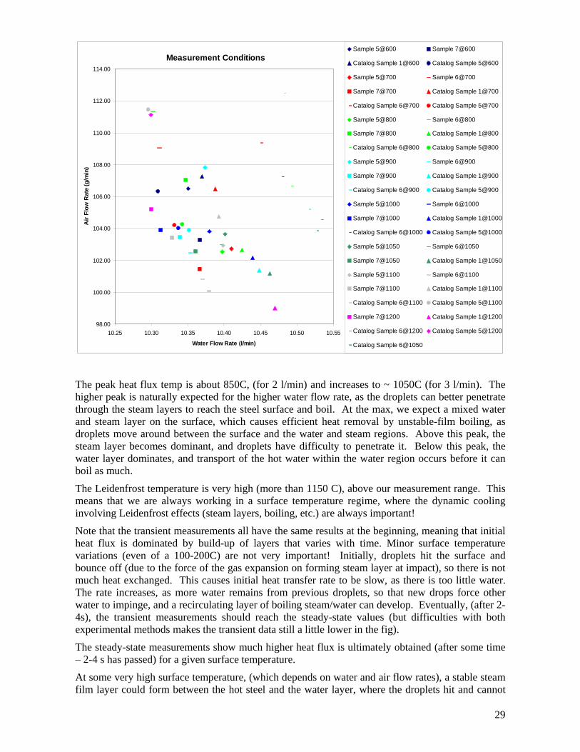
Measurement Conditions

98.00

100.00

102.00

104.00

106.00

108.00

110.00

112.00

114.00

10.25 10.30 10.35 10.40 10.45 10.50 10.55

Water Flow Rate (l/min)

Air

Flow

Rat

e (g

/min

)

Sample 5@600 Sample 7@600

Catalog Sample 1@600 Catalog Sample 5@600

Sample 5@700 Sample 6@700

Sample 7@700 Catalog Sample 1@700

Catalog Sample 6@700 Catalog Sample 5@700

Sample 5@800 Sample 6@800

Sample 7@800 Catalog Sample 1@800

Catalog Sample 6@800 Catalog Sample 5@800

Sample 5@900 Sample 6@900

Sample 7@900 Catalog Sample 1@900

Catalog Sample 6@900 Catalog Sample 5@900

Sample 5@1000 Sample 6@1000

Sample 7@1000 Catalog Sample 1@1000

Catalog Sample 6@1000 Catalog Sample 5@1000

Sample 5@1050 Sample 6@1050

Sample 7@1050 Catalog Sample 1@1050

Sample 5@1100 Sample 6@1100

Sample 7@1100 Catalog Sample 1@1100

Catalog Sample 6@1100 Catalog Sample 5@1100

Sample 7@1200 Catalog Sample 1@1200

Catalog Sample 6@1200 Catalog Sample 5@1200

Catalog Sample 6@1050

The peak heat flux temp is about 850C, (for 2 l/min) and increases to ~ 1050C (for 3 l/min). The higher peak is naturally expected for the higher water flow rate, as the droplets can better penetrate through the steam layers to reach the steel surface and boil. At the max, we expect a mixed water and steam layer on the surface, which causes efficient heat removal by unstable-film boiling, as droplets move around between the surface and the water and steam regions. Above this peak, the steam layer becomes dominant, and droplets have difficulty to penetrate it. Below this peak, the water layer dominates, and transport of the hot water within the water region occurs before it can boil as much.

The Leidenfrost temperature is very high (more than 1150 C), above our measurement range. This means that we are always working in a surface temperature regime, where the dynamic cooling involving Leidenfrost effects (steam layers, boiling, etc.) are always important!

Note that the transient measurements all have the same results at the beginning, meaning that initial heat flux is dominated by build-up of layers that varies with time. Minor surface temperature variations (even of a 100-200C) are not very important! Initially, droplets hit the surface and bounce off (due to the force of the gas expansion on forming steam layer at impact), so there is not much heat exchanged. This causes initial heat transfer rate to be slow, as there is too little water. The rate increases, as more water remains from previous droplets, so that new drops force other water to impinge, and a recirculating layer of boiling steam/water can develop. Eventually, (after 2-4s), the transient measurements should reach the steady-state values (but difficulties with both experimental methods makes the transient data still a little lower in the fig).

The steady-state measurements show much higher heat flux is ultimately obtained (after some time – 2-4 s has passed) for a given surface temperature.

At some very high surface temperature, (which depends on water and air flow rates), a stable steam film layer could form between the hot steel and the water layer, where the droplets hit and cannot

30

penetrate. This gives the lowest heat transfer rate (the Leidenfrost temperature). Increasing temperature eventually increases heat flux due to increased radiation.

The air-mist nozzle has higher heat transfer. It helps to get more use out of the existing water, but forcing droplets further through a water layer, and by mixing the existing water / steam layers. Thus, higher flux is found for a given water flux.

Implications for modelling: when leaving from beneath a roll, if the steel surface becomes “dry”, then the initial impact of the next water spray jet will take the steel through the transient heat-flux cycle (like the transient experiment) for 2-4s. Thus, the heat transfer will depend on casting speed for 2 reasons (changes the time / length of this region, and changes the surface temperature). If there is enough water for the region above the jet to remain wet at all times, then the steady-state heat flux values would likely dominate, and the transient heat flux is simply too small.

Implications of heat transfer mechanism: pressure behind the water droplets is very important, as their impact momentum determines how efficiently heat is transferred. Thus, pressure variations at the nozzle will greatly change the heat removal rate.

Thus, it is important to carefully monitor and control pressure.

References 1. CONTA manual

31

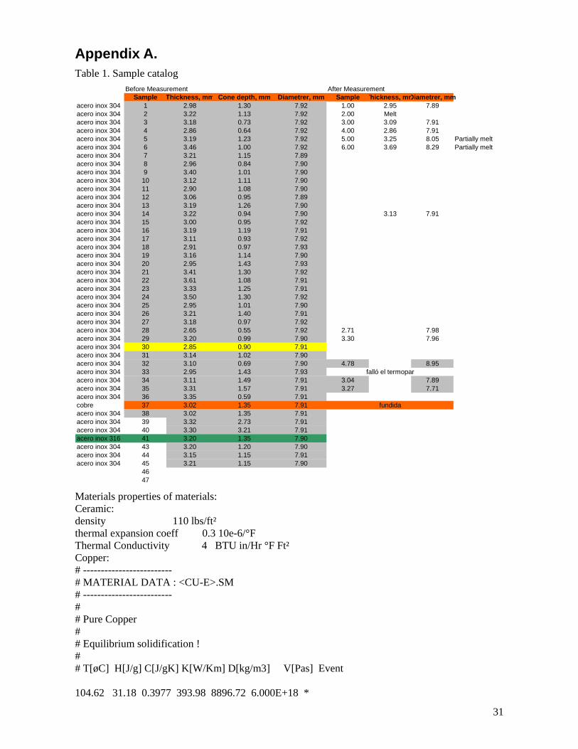
Appendix A. Table 1. Sample catalog

Before Measurement After MeasurementSample Thickness, mm Cone depth, mm Diametrer, mm Sample Thickness, mmDiametrer, mm

acero inox 304 1 2.98 1.30 7.92 1.00 2.95 7.89acero inox 304 2 3.22 1.13 7.92 2.00 Meltacero inox 304 3 3.18 0.73 7.92 3.00 3.09 7.91acero inox 304 4 2.86 0.64 7.92 4.00 2.86 7.91acero inox 304 5 3.19 1.23 7.92 5.00 3.25 8.05 Partially meltacero inox 304 6 3.46 1.00 7.92 6.00 3.69 8.29 Partially meltacero inox 304 7 3.21 1.15 7.89acero inox 304 8 2.96 0.84 7.90acero inox 304 9 3.40 1.01 7.90acero inox 304 10 3.12 1.11 7.90acero inox 304 11 2.90 1.08 7.90acero inox 304 12 3.06 0.95 7.89acero inox 304 13 3.19 1.26 7.90acero inox 304 14 3.22 0.94 7.90 3.13 7.91acero inox 304 15 3.00 0.95 7.92acero inox 304 16 3.19 1.19 7.91acero inox 304 17 3.11 0.93 7.92acero inox 304 18 2.91 0.97 7.93acero inox 304 19 3.16 1.14 7.90acero inox 304 20 2.95 1.43 7.93acero inox 304 21 3.41 1.30 7.92acero inox 304 22 3.61 1.08 7.91acero inox 304 23 3.33 1.25 7.91acero inox 304 24 3.50 1.30 7.92acero inox 304 25 2.95 1.01 7.90acero inox 304 26 3.21 1.40 7.91acero inox 304 27 3.18 0.97 7.92acero inox 304 28 2.65 0.55 7.92 2.71 7.98acero inox 304 29 3.20 0.99 7.90 3.30 7.96acero inox 304 30 2.85 0.90 7.91acero inox 304 31 3.14 1.02 7.90acero inox 304 32 3.10 0.69 7.90 4.78 8.95acero inox 304 33 2.95 1.43 7.93acero inox 304 34 3.11 1.49 7.91 3.04 7.89acero inox 304 35 3.31 1.57 7.91 3.27 7.71acero inox 304 36 3.35 0.59 7.91cobre 37 3.02 1.35 7.91acero inox 304 38 3.02 1.35 7.91acero inox 304 39 3.32 2.73 7.91acero inox 304 40 3.30 3.21 7.91acero inox 316 41 3.20 1.35 7.90acero inox 304 43 3.20 1.20 7.90acero inox 304 44 3.15 1.15 7.91acero inox 304 45 3.21 1.15 7.90

4647

falló el termopar

fundida

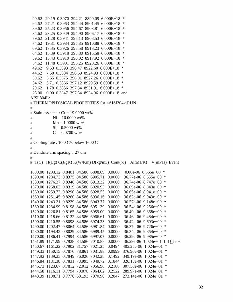
Materials properties of materials: Ceramic: density 110 lbs/ft² thermal expansion coeff 0.3 10e-6/°F Thermal Conductivity 4 BTU in/Hr °F Ft² Copper: # ------------------------- # MATERIAL DATA : <CU-E>.SM # ------------------------- # # Pure Copper # # Equilibrium solidification ! # # T[øC] H[J/g] C[J/gK] K[W/Km] D[kg/m3] V[Pas] Event 104.62 31.18 0.3977 393.98 8896.72 6.000E+18 *

32

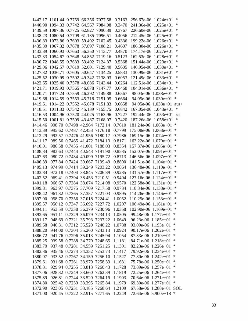
99.62 29.19 0.3970 394.21 8899.09 6.000E+18 * 94.62 27.21 0.3963 394.44 8901.45 6.000E+18 * 89.62 25.23 0.3956 394.67 8903.81 6.000E+18 * 84.62 23.25 0.3949 394.90 8906.17 6.000E+18 * 79.62 21.28 0.3941 395.13 8908.53 6.000E+18 * 74.62 19.31 0.3934 395.35 8910.88 6.000E+18 * 69.62 17.35 0.3926 395.58 8913.23 6.000E+18 * 64.62 15.39 0.3918 395.80 8915.58 6.000E+18 * 59.62 13.43 0.3910 396.02 8917.92 6.000E+18 * 54.62 11.48 0.3901 396.25 8920.26 6.000E+18 * 49.62 9.53 0.3893 396.47 8922.60 6.000E+18 * 44.62 7.58 0.3884 396.69 8924.93 6.000E+18 * 39.62 5.65 0.3875 396.91 8927.26 6.000E+18 * 34.62 3.71 0.3866 397.12 8929.59 6.000E+18 * 29.62 1.78 0.3856 397.34 8931.91 6.000E+18 * 25.00 0.00 0.3847 397.54 8934.06 6.000E+18 end AISI 304L: # THERMOPHYSICAL PROPERTIES for <AISI304>.RUN # # Stainless steel : Cr = 19.0000 wt% # Ni = 10.0000 wt% # Mn = 1.0000 wt% # Si = 0.5000 wt% # C = 0.0700 wt% # # Cooling rate : 10.0 C/s below 1600 C # # Dendrite arm spacing : 27 um # # T(C) H(J/g) C(J/gK) K(W/Km) D(kg/m3) Cont(%) Alfa(1/K) V(mPas) Event 1600.00 1293.12 0.8401 84.586 6898.09 0.0000 0.00e-06 8.565e+00 * 1590.00 1284.73 0.8375 84.586 6905.71 0.0000 36.77e-06 8.655e+00 * 1580.00 1276.37 0.8348 84.586 6913.32 0.0000 36.74e-06 8.747e+00 * 1570.00 1268.03 0.8319 84.586 6920.93 0.0000 36.69e-06 8.843e+00 * 1560.00 1259.73 0.8290 84.586 6928.55 0.0000 36.65e-06 8.941e+00 * 1550.00 1251.45 0.8260 84.586 6936.16 0.0000 36.62e-06 9.043e+00 * 1540.00 1243.21 0.8229 84.586 6943.77 0.0000 36.57e-06 9.148e+00 * 1530.00 1234.99 0.8198 84.586 6951.39 0.0000 36.54e-06 9.256e+00 * 1520.00 1226.81 0.8165 84.586 6959.00 0.0000 36.49e-06 9.368e+00 * 1510.00 1218.66 0.8132 84.586 6966.61 0.0000 36.46e-06 9.484e+00 * 1500.00 1210.55 0.8098 84.586 6974.23 0.0000 36.42e-06 9.603e+00 * 1490.00 1202.47 0.8064 84.586 6981.84 0.0000 36.37e-06 9.726e+00 * 1480.00 1194.42 0.8029 84.586 6989.45 0.0000 36.34e-06 9.854e+00 * 1470.00 1186.41 0.7994 84.586 6997.07 0.0000 36.29e-06 9.985e+00 * 1451.89 1171.99 0.7928 84.586 7010.85 0.0000 36.29e-06 1.024e+01 LIQ_fer+ 1450.67 1161.22 0.7902 81.757 7021.25 0.0494 405.25e-06 1.024e+01 * 1449.33 1150.15 0.7876 78.861 7031.88 0.0999 376.90e-06 1.024e+01 * 1447.92 1139.23 0.7849 76.026 7042.28 0.1492 349.19e-06 1.024e+01 * 1446.84 1131.38 0.7831 73.995 7049.72 0.1844 326.18e-06 1.024e+01 * 1445.73 1123.67 0.7812 72.012 7056.96 0.2188 307.50e-06 1.024e+01 * 1444.58 1116.11 0.7794 70.078 7064.02 0.2522 289.97e-06 1.024e+01 * 1443.39 1108.71 0.7776 68.193 7070.90 0.2847 273.14e-06 1.024e+01 *

33

1442.17 1101.44 0.7759 66.356 7077.58 0.3163 256.67e-06 1.024e+01 * 1440.90 1094.33 0.7742 64.567 7084.08 0.3470 241.36e-06 1.025e+01 * 1439.59 1087.36 0.7725 62.827 7090.39 0.3767 226.60e-06 1.025e+01 * 1438.23 1080.54 0.7709 61.135 7096.51 0.4056 212.45e-06 1.025e+01 * 1436.83 1073.86 0.7693 59.492 7102.45 0.4336 199.22e-06 1.026e+01 * 1435.39 1067.32 0.7678 57.897 7108.21 0.4607 186.30e-06 1.026e+01 * 1433.89 1060.93 0.7663 56.350 7113.77 0.4870 174.17e-06 1.027e+01 * 1432.33 1054.67 0.7648 54.852 7119.16 0.5123 162.53e-06 1.028e+01 * 1430.72 1048.55 0.7633 53.402 7124.37 0.5368 151.44e-06 1.029e+01 * 1429.06 1042.57 0.7619 52.001 7129.40 0.5605 140.95e-06 1.030e+01 * 1427.32 1036.71 0.7605 50.647 7134.25 0.5833 130.99e-06 1.031e+01 * 1425.52 1030.99 0.7592 49.342 7138.93 0.6053 121.49e-06 1.033e+01 * 1423.65 1025.40 0.7578 48.086 7143.44 0.6264 112.51e-06 1.034e+01 * 1421.71 1019.93 0.7565 46.878 7147.77 0.6468 104.01e-06 1.036e+01 * 1420.71 1017.24 0.7559 46.292 7149.88 0.6567 98.03e-06 1.038e+01 * 1419.68 1014.59 0.7553 45.718 7151.95 0.6664 94.05e-06 1.039e+01 * 1419.61 1014.22 0.7552 45.678 7151.83 0.6658 94.05e-06 1.038e+01 aus+ 1418.51 1011.33 0.7542 45.139 7155.75 0.6842 167.05e-06 1.043e+01 * 1416.53 1004.96 0.7520 44.025 7163.96 0.7227 192.44e-06 1.053e+01 zst 1415.50 1001.81 0.7509 43.487 7168.07 0.7420 187.26e-06 1.058e+01 * 1414.46 998.70 0.7498 42.964 7172.14 0.7610 181.24e-06 1.063e+01 * 1413.39 995.62 0.7487 42.453 7176.18 0.7799 175.08e-06 1.068e+01 * 1412.29 992.57 0.7476 41.956 7180.17 0.7986 169.15e-06 1.074e+01 * 1411.17 989.56 0.7465 41.472 7184.13 0.8171 163.22e-06 1.079e+01 * 1410.01 986.58 0.7455 41.001 7188.03 0.8354 157.37e-06 1.085e+01 * 1408.84 983.63 0.7444 40.543 7191.90 0.8535 152.07e-06 1.091e+01 * 1407.63 980.72 0.7434 40.099 7195.72 0.8713 146.56e-06 1.097e+01 * 1406.39 977.84 0.7424 39.667 7199.49 0.8890 141.51e-06 1.104e+01 * 1405.13 974.99 0.7414 39.249 7203.22 0.9064 136.48e-06 1.110e+01 * 1403.84 972.18 0.7404 38.845 7206.89 0.9235 131.57e-06 1.117e+01 * 1402.52 969.41 0.7394 38.453 7210.51 0.9404 127.16e-06 1.124e+01 * 1401.18 966.67 0.7384 38.074 7214.08 0.9570 122.58e-06 1.131e+01 * 1399.81 963.97 0.7375 37.709 7217.58 0.9734 118.34e-06 1.138e+01 * 1398.42 961.32 0.7365 37.357 7221.03 0.9895 114.26e-06 1.146e+01 * 1397.00 958.70 0.7356 37.018 7224.41 1.0052 110.25e-06 1.153e+01 * 1395.57 956.12 0.7347 36.692 7227.72 1.0207 106.49e-06 1.161e+01 * 1394.11 953.59 0.7338 36.379 7230.96 1.0358 102.90e-06 1.169e+01 * 1392.65 951.11 0.7329 36.079 7234.13 1.0505 99.48e-06 1.177e+01 * 1391.17 948.69 0.7321 35.793 7237.22 1.0649 96.23e-06 1.185e+01 * 1389.68 946.31 0.7312 35.520 7240.22 1.0788 93.09e-06 1.193e+01 * 1388.20 944.00 0.7304 35.260 7243.13 1.0924 90.17e-06 1.202e+01 * 1386.72 941.76 0.7296 35.013 7245.94 1.1054 87.33e-06 1.210e+01 * 1385.25 939.58 0.7288 34.779 7248.65 1.1181 84.71e-06 1.218e+01 * 1383.79 937.48 0.7281 34.559 7251.25 1.1301 82.23e-06 1.226e+01 * 1382.36 935.46 0.7274 34.352 7253.73 1.1417 79.92e-06 1.234e+01 * 1380.97 933.52 0.7267 34.159 7256.10 1.1527 77.80e-06 1.242e+01 * 1379.61 931.68 0.7261 33.979 7258.33 1.1631 75.78e-06 1.250e+01 * 1378.31 929.94 0.7255 33.813 7260.43 1.1728 73.89e-06 1.257e+01 * 1377.06 928.32 0.7249 33.660 7262.39 1.1819 72.25e-06 1.264e+01 * 1375.89 926.81 0.7244 33.520 7264.19 1.1903 70.64e-06 1.271e+01 * 1374.80 925.42 0.7239 33.395 7265.84 1.1979 69.30e-06 1.277e+01 * 1372.90 923.05 0.7231 33.185 7268.64 1.2109 67.58e-06 1.288e+01 SOL 1371.00 920.45 0.7222 32.915 7271.65 1.2249 72.64e-06 5.900e+18 *

34

1370.00 919.60 0.7219 32.902 7272.62 1.2294 44.36e-06 5.900e+18 * 1369.00 918.77 0.7216 32.888 7273.51 1.2335 41.00e-06 5.900e+18 * 1368.00 917.94 0.7213 32.875 7274.39 1.2376 40.30e-06 5.900e+18 * 1367.00 917.11 0.7210 32.861 7275.26 1.2417 39.96e-06 5.900e+18 * 1366.00 916.29 0.7207 32.848 7276.13 1.2457 39.60e-06 5.900e+18 * 1365.00 915.47 0.7204 32.834 7276.99 1.2497 39.28e-06 5.900e+18 * 1364.00 914.65 0.7200 32.821 7277.84 1.2536 38.92e-06 5.900e+18 * 1363.00 913.84 0.7197 32.807 7278.68 1.2575 38.71e-06 5.900e+18 * 1362.00 913.02 0.7194 32.794 7279.52 1.2614 38.41e-06 5.900e+18 * 1361.00 912.21 0.7191 32.780 7280.35 1.2653 38.07e-06 5.900e+18 * 1360.00 911.40 0.7188 32.767 7281.18 1.2691 37.82e-06 5.900e+18 * 1359.00 910.59 0.7185 32.754 7282.00 1.2729 37.53e-06 5.900e+18 * 1358.00 909.78 0.7182 32.740 7282.81 1.2767 37.24e-06 5.900e+18 * 1357.00 908.98 0.7179 32.727 7283.62 1.2804 37.01e-06 5.900e+18 * 1356.00 908.18 0.7177 32.713 7284.42 1.2841 36.71e-06 5.900e+18 * 1355.00 907.38 0.7174 32.700 7285.22 1.2878 36.42e-06 5.900e+18 * 1354.00 906.58 0.7171 32.686 7286.01 1.2915 36.17e-06 5.900e+18 * 1353.00 905.78 0.7168 32.673 7286.79 1.2951 35.96e-06 5.900e+18 * 1352.00 904.99 0.7165 32.659 7287.58 1.2987 35.76e-06 5.900e+18 * 1351.00 904.19 0.7162 32.646 7288.35 1.3023 35.44e-06 5.900e+18 * 1350.00 903.40 0.7159 32.633 7289.12 1.3059 35.22e-06 5.900e+18 * 1349.00 902.61 0.7156 32.619 7289.89 1.3095 35.06e-06 5.900e+18 * 1348.00 901.82 0.7153 32.606 7290.65 1.3130 34.81e-06 5.900e+18 * 1347.00 901.04 0.7151 32.592 7291.41 1.3165 34.58e-06 5.900e+18 * 1346.00 900.25 0.7148 32.579 7292.16 1.3200 34.37e-06 5.900e+18 * 1345.00 899.47 0.7145 32.565 7292.90 1.3234 34.17e-06 5.900e+18 * 1344.00 898.69 0.7142 32.552 7293.65 1.3269 33.92e-06 5.900e+18 * 1343.00 897.90 0.7139 32.539 7294.38 1.3303 33.72e-06 5.900e+18 * 1342.00 897.12 0.7137 32.525 7295.12 1.3337 33.56e-06 5.900e+18 * 1341.00 896.35 0.7134 32.512 7295.85 1.3371 33.35e-06 5.900e+18 * 1340.00 895.57 0.7131 32.498 7296.57 1.3404 33.13e-06 5.900e+18 * 1339.00 894.80 0.7128 32.485 7297.30 1.3438 33.01e-06 5.900e+18 * 1338.00 894.02 0.7126 32.471 7298.01 1.3471 32.76e-06 5.900e+18 * 1337.00 893.25 0.7123 32.458 7298.73 1.3504 32.65e-06 5.900e+18 * 1336.00 892.48 0.7120 32.445 7299.44 1.3537 32.47e-06 5.900e+18 * 1335.00 891.71 0.7117 32.431 7300.15 1.3570 32.24e-06 5.900e+18 * 1334.00 890.94 0.7115 32.418 7300.85 1.3602 32.10e-06 5.900e+18 * 1333.00 890.17 0.7112 32.404 7301.55 1.3634 31.95e-06 5.900e+18 * 1332.00 889.41 0.7109 32.391 7302.24 1.3667 31.72e-06 5.900e+18 * 1331.00 888.64 0.7107 32.377 7302.94 1.3699 31.65e-06 5.900e+18 * 1330.00 887.88 0.7104 32.364 7303.63 1.3731 31.47e-06 5.900e+18 * 1329.00 887.12 0.7101 32.351 7304.31 1.3762 31.24e-06 5.900e+18 * 1328.00 886.35 0.7099 32.337 7305.00 1.3794 31.22e-06 5.900e+18 * 1327.00 885.59 0.7096 32.324 7305.67 1.3825 30.95e-06 5.900e+18 * 1326.00 884.84 0.7093 32.310 7306.35 1.3857 30.85e-06 5.900e+18 * 1325.00 884.08 0.7091 32.297 7307.02 1.3888 30.76e-06 5.900e+18 * 1324.00 883.32 0.7088 32.284 7307.69 1.3919 30.60e-06 5.900e+18 * 1323.00 882.56 0.7085 32.270 7308.36 1.3950 30.42e-06 5.900e+18 * 1322.00 881.81 0.7083 32.257 7309.03 1.3980 30.29e-06 5.900e+18 s50 1320.00 880.31 0.7078 32.230 7310.33 1.4041 29.85e-06 5.900e+18 * 1315.00 876.56 0.7065 32.163 7313.58 1.4191 29.63e-06 5.900e+18 * 1310.00 872.82 0.7052 32.096 7316.81 1.4340 29.41e-06 5.900e+18 * 1305.00 869.11 0.7039 32.029 7319.97 1.4486 28.81e-06 5.900e+18 *

35

1300.00 865.42 0.7027 31.962 7323.08 1.4630 28.27e-06 5.900e+18 * 1295.00 861.75 0.7014 31.896 7326.13 1.4771 27.76e-06 5.900e+18 * 1290.00 858.10 0.7002 31.829 7329.13 1.4909 27.33e-06 5.900e+18 * 1285.00 854.46 0.6990 31.762 7332.09 1.5046 26.91e-06 5.900e+18 * 1280.00 850.84 0.6978 31.695 7335.01 1.5181 26.55e-06 5.900e+18 * 1275.00 847.24 0.6966 31.629 7337.90 1.5314 26.22e-06 5.900e+18 * 1270.00 843.65 0.6954 31.562 7340.75 1.5445 25.89e-06 5.900e+18 * 1265.00 840.07 0.6943 31.495 7343.57 1.5575 25.62e-06 5.900e+18 * 1260.00 836.50 0.6931 31.429 7346.36 1.5704 25.35e-06 5.900e+18 * 1255.00 832.95 0.6919 31.362 7349.13 1.5831 25.11e-06 5.900e+18 * 1250.00 829.41 0.6908 31.296 7351.87 1.5958 24.87e-06 5.900e+18 * 1245.00 825.88 0.6896 31.229 7354.59 1.6083 24.68e-06 5.900e+18 * 1240.00 822.36 0.6885 31.163 7357.29 1.6207 24.47e-06 5.900e+18 * 1235.00 818.85 0.6874 31.096 7359.97 1.6331 24.29e-06 5.900e+18 * 1230.00 815.35 0.6862 31.030 7362.64 1.6454 24.13e-06 5.900e+18 * 1225.00 811.86 0.6851 30.964 7365.28 1.6575 23.95e-06 5.900e+18 * 1220.00 808.38 0.6840 30.897 7367.91 1.6696 23.81e-06 5.900e+18 * 1215.00 804.91 0.6829 30.831 7370.53 1.6817 23.66e-06 5.900e+18 * 1210.00 801.45 0.6818 30.765 7373.13 1.6936 23.53e-06 5.900e+18 * 1205.00 797.99 0.6807 30.699 7375.72 1.7055 23.41e-06 5.900e+18 * 1200.00 794.54 0.6796 30.632 7378.30 1.7174 23.28e-06 5.900e+18 * 1195.00 791.11 0.6785 30.566 7380.86 1.7291 23.18e-06 5.900e+18 * 1190.00 787.67 0.6774 30.500 7383.41 1.7409 23.05e-06 5.900e+18 * 1185.00 784.25 0.6763 30.434 7385.96 1.7525 22.95e-06 5.900e+18 * 1180.00 780.84 0.6752 30.368 7388.49 1.7642 22.86e-06 5.900e+18 * 1175.00 777.43 0.6742 30.302 7391.01 1.7758 22.76e-06 5.900e+18 * 1170.00 774.02 0.6731 30.236 7393.53 1.7873 22.67e-06 5.900e+18 * 1165.00 770.63 0.6720 30.170 7396.03 1.7988 22.59e-06 5.900e+18 * 1160.00 767.24 0.6709 30.104 7398.53 1.8102 22.50e-06 5.900e+18 * 1155.00 763.86 0.6699 30.038 7401.02 1.8217 22.43e-06 5.900e+18 * 1150.00 760.49 0.6688 29.973 7403.50 1.8330 22.35e-06 5.900e+18 * 1145.00 757.12 0.6678 29.907 7405.97 1.8444 22.28e-06 5.900e+18 * 1140.00 753.76 0.6667 29.841 7408.44 1.8557 22.22e-06 5.900e+18 * 1135.00 750.41 0.6657 29.775 7410.90 1.8670 22.13e-06 5.900e+18 * 1130.00 747.06 0.6646 29.710 7413.36 1.8782 22.08e-06 5.900e+18 * 1125.00 743.72 0.6636 29.644 7415.80 1.8894 22.01e-06 5.900e+18 * 1120.00 740.38 0.6626 29.578 7418.25 1.9006 21.95e-06 5.900e+18 * 1115.00 737.05 0.6615 29.513 7420.68 1.9118 21.90e-06 5.900e+18 * 1110.00 733.73 0.6605 29.447 7423.11 1.9229 21.83e-06 5.900e+18 * 1105.00 730.41 0.6595 29.382 7425.54 1.9340 21.79e-06 5.900e+18 * 1100.00 727.10 0.6584 29.316 7427.96 1.9451 21.73e-06 5.900e+18 * 1095.00 723.80 0.6574 29.251 7430.38 1.9561 21.69e-06 5.900e+18 * 1090.00 720.50 0.6564 29.185 7432.79 1.9672 21.63e-06 5.900e+18 * 1085.00 717.20 0.6554 29.120 7435.20 1.9782 21.58e-06 5.900e+18 * 1080.00 713.92 0.6544 29.054 7437.60 1.9891 21.54e-06 5.900e+18 * 1075.00 710.63 0.6534 28.989 7440.00 2.0001 21.48e-06 5.900e+18 * 1070.00 707.36 0.6523 28.924 7442.39 2.0110 21.45e-06 5.900e+18 * 1065.00 704.09 0.6513 28.859 7444.78 2.0220 21.40e-06 5.900e+18 * 1060.00 700.82 0.6503 28.793 7447.16 2.0329 21.36e-06 5.900e+18 * 1055.00 697.56 0.6493 28.728 7449.55 2.0437 21.32e-06 5.900e+18 * 1050.00 694.31 0.6483 28.663 7451.92 2.0546 21.28e-06 5.900e+18 * 1045.00 691.06 0.6473 28.598 7454.30 2.0654 21.24e-06 5.900e+18 * 1040.00 687.82 0.6464 28.533 7456.67 2.0762 21.20e-06 5.900e+18 *

36

1035.00 684.58 0.6454 28.468 7459.04 2.0870 21.16e-06 5.900e+18 * 1030.00 681.35 0.6444 28.403 7461.40 2.0978 21.12e-06 5.900e+18 * 1025.00 678.12 0.6434 28.338 7463.76 2.1086 21.09e-06 5.900e+18 * 1020.00 674.90 0.6424 28.273 7466.12 2.1193 21.05e-06 5.900e+18 * 1015.00 671.68 0.6414 28.208 7468.47 2.1301 21.02e-06 5.900e+18 * 1010.00 668.47 0.6405 28.143 7470.82 2.1408 20.99e-06 5.900e+18 * 1005.00 665.26 0.6395 28.078 7473.17 2.1515 20.96e-06 5.900e+18 * 1000.00 662.06 0.6385 28.013 7475.52 2.1622 20.91e-06 5.900e+18 * 995.00 658.86 0.6376 27.948 7477.86 2.1728 20.89e-06 5.900e+18 * 990.00 655.67 0.6366 27.884 7480.20 2.1835 20.86e-06 5.900e+18 * 985.00 652.49 0.6356 27.819 7482.53 2.1941 20.82e-06 5.900e+18 * 980.00 649.31 0.6347 27.754 7484.87 2.2047 20.79e-06 5.900e+18 * 975.00 646.13 0.6337 27.690 7487.20 2.2154 20.76e-06 5.900e+18 * 970.00 642.96 0.6328 27.625 7489.53 2.2260 20.74e-06 5.900e+18 * 965.00 639.80 0.6318 27.560 7491.85 2.2365 20.70e-06 5.900e+18 * 960.00 636.64 0.6309 27.496 7494.17 2.2471 20.67e-06 5.900e+18 * 955.00 633.48 0.6300 27.431 7496.49 2.2576 20.63e-06 5.900e+18 * 950.00 630.33 0.6290 27.367 7498.81 2.2682 20.61e-06 5.900e+18 * 945.00 627.18 0.6281 27.302 7501.13 2.2787 20.57e-06 5.900e+18 * 940.00 624.04 0.6271 27.238 7503.44 2.2892 20.55e-06 5.900e+18 * 935.00 620.91 0.6262 27.174 7505.75 2.2997 20.52e-06 5.900e+18 * 930.00 617.78 0.6253 27.109 7508.06 2.3102 20.49e-06 5.900e+18 * 925.00 614.65 0.6244 27.045 7510.36 2.3207 20.46e-06 5.900e+18 * 920.00 611.53 0.6234 26.981 7512.66 2.3311 20.43e-06 5.900e+18 * 915.00 608.41 0.6225 26.917 7514.96 2.3415 20.41e-06 5.900e+18 * 910.00 605.30 0.6216 26.852 7517.26 2.3520 20.38e-06 5.900e+18 * 905.00 602.19 0.6207 26.788 7519.55 2.3624 20.34e-06 5.900e+18 * 900.00 599.09 0.6198 26.724 7521.85 2.3728 20.32e-06 5.900e+18 * 895.00 595.99 0.6189 26.660 7524.13 2.3832 20.28e-06 5.900e+18 * 890.00 592.90 0.6180 26.596 7526.42 2.3935 20.25e-06 5.900e+18 * 885.00 589.81 0.6171 26.532 7528.70 2.4039 20.23e-06 5.900e+18 * 880.00 586.72 0.6162 26.468 7530.98 2.4142 20.19e-06 5.900e+18 * 875.00 583.65 0.6153 26.404 7533.26 2.4245 20.16e-06 5.900e+18 * 870.00 580.57 0.6144 26.340 7535.54 2.4349 20.12e-06 5.900e+18 * 865.00 577.50 0.6136 26.276 7537.81 2.4451 20.09e-06 5.900e+18 * 860.00 574.43 0.6127 26.212 7540.08 2.4554 20.07e-06 5.900e+18 * 855.00 571.37 0.6118 26.148 7542.34 2.4657 20.04e-06 5.900e+18 * 850.00 568.31 0.6110 26.085 7544.61 2.4759 20.00e-06 5.900e+18 * 845.00 565.26 0.6101 26.021 7546.87 2.4862 19.98e-06 5.900e+18 * 840.00 562.21 0.6092 25.957 7549.13 2.4964 19.94e-06 5.900e+18 * 835.00 559.17 0.6084 25.893 7551.38 2.5066 19.93e-06 5.900e+18 * 830.00 556.13 0.6075 25.830 7553.63 2.5168 19.88e-06 5.900e+18 * 825.00 553.09 0.6067 25.766 7555.88 2.5270 19.85e-06 5.900e+18 * 820.00 550.06 0.6059 25.702 7558.13 2.5371 19.81e-06 5.900e+18 * 815.00 547.03 0.6051 25.639 7560.37 2.5473 19.79e-06 5.900e+18 * 800.00 537.98 0.6026 25.448 7567.10 2.5777 19.76e-06 5.900e+18 endH 795.00 535.04 0.6018 25.385 7569.20 2.5872 18.53e-06 5.900e+18 * 790.00 532.03 0.6010 25.322 7571.44 2.5973 19.71e-06 5.900e+18 * 785.00 529.03 0.6002 25.258 7573.67 2.6074 19.68e-06 5.900e+18 * 780.00 526.03 0.5994 25.195 7575.91 2.6175 19.67e-06 5.900e+18 * 775.00 523.03 0.5987 25.132 7578.14 2.6276 19.66e-06 5.900e+18 * 770.00 520.04 0.5979 25.068 7580.37 2.6376 19.63e-06 5.900e+18 * 765.00 517.05 0.5971 25.005 7582.61 2.6477 19.63e-06 5.900e+18 *

37

760.00 514.07 0.5964 24.942 7584.84 2.6578 19.60e-06 5.900e+18 * 755.00 511.09 0.5956 24.879 7587.07 2.6678 19.59e-06 5.900e+18 * 750.00 508.11 0.5949 24.816 7589.29 2.6779 19.58e-06 5.900e+18 * 745.00 505.14 0.5942 24.753 7591.52 2.6879 19.56e-06 5.900e+18 * 740.00 502.17 0.5934 24.690 7593.75 2.6979 19.54e-06 5.900e+18 * 735.00 499.20 0.5927 24.627 7595.97 2.7080 19.53e-06 5.900e+18 * 730.00 496.24 0.5920 24.564 7598.19 2.7180 19.51e-06 5.900e+18 * 725.00 493.28 0.5914 24.501 7600.42 2.7280 19.50e-06 5.900e+18 * 720.00 490.33 0.5907 24.438 7602.64 2.7380 19.48e-06 5.900e+18 * 715.00 487.38 0.5900 24.375 7604.86 2.7480 19.46e-06 5.900e+18 * 710.00 484.43 0.5894 24.312 7607.08 2.7580 19.45e-06 5.900e+18 * 705.00 481.48 0.5888 24.249 7609.29 2.7680 19.43e-06 5.900e+18 * 700.00 478.54 0.5882 24.186 7611.51 2.7780 19.42e-06 5.900e+18 * 695.00 475.60 0.5876 24.124 7613.72 2.7879 19.40e-06 5.900e+18 * 690.00 472.66 0.5870 24.061 7615.94 2.7979 19.38e-06 5.900e+18 * 685.00 469.73 0.5865 23.998 7618.15 2.8078 19.37e-06 5.900e+18 * 680.00 466.80 0.5860 23.936 7620.36 2.8178 19.35e-06 5.900e+18 * 675.00 463.87 0.5855 23.873 7622.57 2.8277 19.33e-06 5.900e+18 * 670.00 460.94 0.5851 23.811 7624.78 2.8377 19.32e-06 5.900e+18 * 665.00 458.02 0.5846 23.748 7626.99 2.8476 19.30e-06 5.900e+18 * 660.00 455.10 0.5843 23.685 7629.20 2.8575 19.29e-06 5.900e+18 * 655.00 452.18 0.5839 23.623 7631.40 2.8674 19.27e-06 5.900e+18 * 650.00 449.26 0.5836 23.561 7633.61 2.8773 19.26e-06 5.900e+18 * 645.00 446.34 0.5834 23.498 7635.81 2.8872 19.24e-06 5.900e+18 * 642.44 444.85 0.5890 23.466 7636.94 2.8923 19.23e-06 5.900e+18 cur 640.00 443.41 0.5882 23.436 7638.01 2.8971 19.23e-06 5.900e+18 * 635.00 440.47 0.5868 23.373 7640.21 2.9070 19.20e-06 5.900e+18 * 630.00 437.54 0.5854 23.311 7642.41 2.9169 19.20e-06 5.900e+18 * 625.00 434.62 0.5840 23.249 7644.61 2.9267 19.17e-06 5.900e+18 * 620.00 431.70 0.5826 23.187 7646.81 2.9366 19.16e-06 5.900e+18 * 615.00 428.79 0.5812 23.124 7649.01 2.9464 19.15e-06 5.900e+18 * 610.00 425.89 0.5799 23.062 7651.20 2.9563 19.13e-06 5.900e+18 * 605.00 423.00 0.5786 23.000 7653.40 2.9661 19.12e-06 5.900e+18 * 600.00 420.11 0.5773 22.938 7655.59 2.9760 19.10e-06 5.900e+18 * 595.00 417.22 0.5760 22.876 7657.78 2.9858 19.09e-06 5.900e+18 * 590.00 414.35 0.5747 22.814 7659.97 2.9956 19.06e-06 5.900e+18 * 585.00 411.48 0.5735 22.752 7662.16 3.0054 19.05e-06 5.900e+18 * 580.00 408.61 0.5722 22.690 7664.35 3.0152 19.04e-06 5.900e+18 * 575.00 405.75 0.5710 22.628 7666.53 3.0250 19.02e-06 5.900e+18 * 570.00 402.90 0.5698 22.566 7668.72 3.0348 19.01e-06 5.900e+18 * 565.00 400.06 0.5686 22.504 7670.91 3.0446 18.99e-06 5.900e+18 * 560.00 397.22 0.5674 22.443 7673.09 3.0544 18.97e-06 5.900e+18 * 555.00 394.38 0.5663 22.381 7675.27 3.0641 18.96e-06 5.900e+18 * 550.00 391.55 0.5651 22.319 7677.45 3.0739 18.94e-06 5.900e+18 * 545.00 388.73 0.5640 22.257 7679.63 3.0837 18.93e-06 5.900e+18 * 540.00 385.91 0.5628 22.196 7681.81 3.0934 18.91e-06 5.900e+18 * 535.00 383.10 0.5617 22.134 7683.99 3.1032 18.90e-06 5.900e+18 * 530.00 380.30 0.5606 22.072 7686.17 3.1129 18.88e-06 5.900e+18 * 525.00 377.50 0.5595 22.011 7688.34 3.1226 18.87e-06 5.900e+18 * 520.00 374.70 0.5584 21.949 7690.51 3.1323 18.85e-06 5.900e+18 * 515.00 371.91 0.5573 21.888 7692.69 3.1420 18.84e-06 5.900e+18 * 510.00 369.13 0.5562 21.826 7694.86 3.1518 18.82e-06 5.900e+18 * 505.00 366.35 0.5551 21.765 7697.03 3.1614 18.80e-06 5.900e+18 *

38

500.00 363.58 0.5541 21.703 7699.20 3.1711 18.79e-06 5.900e+18 * 495.00 360.81 0.5530 21.642 7701.37 3.1808 18.77e-06 5.900e+18 * 490.00 358.05 0.5519 21.581 7703.54 3.1905 18.77e-06 5.900e+18 * 485.00 355.29 0.5509 21.519 7705.70 3.2002 18.73e-06 5.900e+18 * 480.00 352.54 0.5498 21.458 7707.87 3.2098 18.73e-06 5.900e+18 * 475.00 349.79 0.5488 21.397 7710.03 3.2195 18.71e-06 5.900e+18 * 470.00 347.05 0.5478 21.336 7712.19 3.2291 18.70e-06 5.900e+18 * 465.00 344.31 0.5467 21.274 7714.35 3.2388 18.68e-06 5.900e+18 * 460.00 341.58 0.5457 21.213 7716.51 3.2484 18.67e-06 5.900e+18 * 455.00 338.86 0.5447 21.152 7718.67 3.2580 18.64e-06 5.900e+18 * 450.00 336.14 0.5437 21.091 7720.83 3.2677 18.63e-06 5.900e+18 * 445.00 333.42 0.5427 21.030 7722.99 3.2773 18.63e-06 5.900e+18 * 440.00 330.71 0.5417 20.969 7725.14 3.2869 18.60e-06 5.900e+18 * 435.00 328.00 0.5407 20.908 7727.30 3.2965 18.59e-06 5.900e+18 * 430.00 325.30 0.5397 20.847 7729.45 3.3061 18.58e-06 5.900e+18 * 425.00 322.61 0.5387 20.786 7731.60 3.3157 18.56e-06 5.900e+18 * 420.00 319.92 0.5377 20.725 7733.75 3.3252 18.54e-06 5.900e+18 * 415.00 317.23 0.5367 20.664 7735.90 3.3348 18.53e-06 5.900e+18 * 410.00 314.55 0.5357 20.604 7738.05 3.3444 18.51e-06 5.900e+18 * 405.00 311.87 0.5347 20.543 7740.20 3.3539 18.50e-06 5.900e+18 * 400.00 309.20 0.5337 20.482 7742.34 3.3635 18.49e-06 5.900e+18 * 395.00 306.54 0.5328 20.421 7744.49 3.3730 18.47e-06 5.900e+18 * 390.00 303.87 0.5318 20.361 7746.63 3.3826 18.45e-06 5.900e+18 * 385.00 301.22 0.5308 20.300 7748.77 3.3921 18.44e-06 5.900e+18 * 380.00 298.57 0.5298 20.240 7750.92 3.4016 18.42e-06 5.900e+18 * 375.00 295.92 0.5289 20.179 7753.06 3.4111 18.41e-06 5.900e+18 * 370.00 293.28 0.5279 20.118 7755.19 3.4207 18.39e-06 5.900e+18 * 365.00 290.64 0.5269 20.058 7757.33 3.4302 18.37e-06 5.900e+18 * 360.00 288.01 0.5260 19.997 7759.47 3.4397 18.37e-06 5.900e+18 * 355.00 285.38 0.5250 19.937 7761.60 3.4491 18.34e-06 5.900e+18 * 350.00 282.76 0.5240 19.877 7763.74 3.4586 18.33e-06 5.900e+18 * 345.00 280.14 0.5231 19.816 7765.87 3.4681 18.32e-06 5.900e+18 * 340.00 277.53 0.5221 19.756 7768.00 3.4776 18.30e-06 5.900e+18 * 335.00 274.92 0.5212 19.696 7770.14 3.4870 18.29e-06 5.900e+18 * 330.00 272.32 0.5202 19.635 7772.27 3.4965 18.27e-06 5.900e+18 * 325.00 269.72 0.5192 19.575 7774.39 3.5059 18.25e-06 5.900e+18 * 320.00 267.12 0.5183 19.515 7776.52 3.5154 18.24e-06 5.900e+18 * 315.00 264.53 0.5173 19.455 7778.65 3.5248 18.22e-06 5.900e+18 * 310.00 261.95 0.5164 19.395 7780.77 3.5342 18.21e-06 5.900e+18 * 305.00 259.37 0.5154 19.335 7782.90 3.5436 18.19e-06 5.900e+18 * 300.00 256.80 0.5144 19.275 7785.02 3.5531 18.19e-06 5.900e+18 * 295.00 254.23 0.5135 19.215 7787.14 3.5625 18.16e-06 5.900e+18 * 290.00 251.66 0.5125 19.155 7789.26 3.5719 18.15e-06 5.900e+18 * 285.00 249.10 0.5116 19.095 7791.38 3.5813 18.14e-06 5.900e+18 * 280.00 246.55 0.5106 19.035 7793.50 3.5906 18.12e-06 5.900e+18 * 275.00 244.00 0.5096 18.975 7795.61 3.6000 18.11e-06 5.900e+18 * 270.00 241.45 0.5087 18.915 7797.73 3.6094 18.09e-06 5.900e+18 * 265.00 238.91 0.5077 18.855 7799.84 3.6188 18.08e-06 5.900e+18 * 260.00 236.37 0.5067 18.795 7801.96 3.6281 18.06e-06 5.900e+18 * 255.00 233.84 0.5057 18.736 7804.07 3.6375 18.05e-06 5.900e+18 * 250.00 231.32 0.5048 18.676 7806.18 3.6468 18.03e-06 5.900e+18 * 245.00 228.79 0.5038 18.616 7808.29 3.6561 18.02e-06 5.900e+18 * 240.00 226.28 0.5028 18.557 7810.40 3.6655 18.00e-06 5.900e+18 *

39

235.00 223.77 0.5018 18.497 7812.51 3.6748 17.99e-06 5.900e+18 * 230.00 221.26 0.5008 18.437 7814.61 3.6841 17.97e-06 5.900e+18 * 225.00 218.76 0.4998 18.378 7816.72 3.6934 17.96e-06 5.900e+18 * 220.00 216.26 0.4988 18.318 7818.82 3.7027 17.94e-06 5.900e+18 * 215.00 213.77 0.4978 18.259 7820.92 3.7120 17.92e-06 5.900e+18 * 210.00 211.28 0.4968 18.199 7823.03 3.7213 17.91e-06 5.900e+18 * 205.00 208.80 0.4958 18.140 7825.13 3.7306 17.90e-06 5.900e+18 * 200.00 206.33 0.4948 18.081 7827.23 3.7399 17.88e-06 5.900e+18 * 195.00 203.85 0.4938 18.021 7829.32 3.7491 17.87e-06 5.900e+18 * 190.00 201.39 0.4927 17.962 7831.42 3.7584 17.85e-06 5.900e+18 * 185.00 198.93 0.4917 17.903 7833.52 3.7676 17.84e-06 5.900e+18 * 180.00 196.47 0.4907 17.843 7835.61 3.7769 17.83e-06 5.900e+18 * 175.00 194.02 0.4896 17.784 7837.70 3.7861 17.81e-06 5.900e+18 * 170.00 191.57 0.4886 17.725 7839.80 3.7954 17.80e-06 5.900e+18 * 165.00 189.13 0.4875 17.666 7841.89 3.8046 17.77e-06 5.900e+18 * 160.00 186.70 0.4864 17.607 7843.98 3.8138 17.77e-06 5.900e+18 * 155.00 184.27 0.4853 17.548 7846.07 3.8230 17.74e-06 5.900e+18 * 150.00 181.85 0.4842 17.489 7848.15 3.8322 17.74e-06 5.900e+18 * 145.00 179.43 0.4831 17.430 7850.24 3.8414 17.72e-06 5.900e+18 * 140.00 177.01 0.4820 17.371 7852.33 3.8506 17.71e-06 5.900e+18 * 135.00 174.61 0.4809 17.312 7854.41 3.8598 17.69e-06 5.900e+18 * 130.00 172.21 0.4797 17.253 7856.49 3.8690 17.68e-06 5.900e+18 * 125.00 169.81 0.4786 17.194 7858.57 3.8782 17.66e-06 5.900e+18 * 120.00 167.42 0.4774 17.135 7860.65 3.8873 17.64e-06 5.900e+18 * 115.00 165.04 0.4762 17.076 7862.73 3.8965 17.64e-06 5.900e+18 * 110.00 162.66 0.4750 17.018 7864.81 3.9056 17.61e-06 5.900e+18 * 105.00 160.29 0.4738 16.959 7866.89 3.9148 17.61e-06 5.900e+18 * 100.00 157.92 0.4725 16.900 7868.96 3.9239 17.59e-06 5.900e+18 * 95.00 155.56 0.4712 16.842 7871.04 3.9331 17.58e-06 5.900e+18 * 90.00 153.21 0.4700 16.783 7873.11 3.9422 17.56e-06 5.900e+18 * 85.00 150.86 0.4687 16.724 7875.18 3.9513 17.54e-06 5.900e+18 * 80.00 148.52 0.4673 16.666 7877.26 3.9604 17.53e-06 5.900e+18 * 75.00 146.19 0.4660 16.607 7879.33 3.9695 17.52e-06 5.900e+18 * 70.00 143.86 0.4646 16.549 7881.39 3.9786 17.50e-06 5.900e+18 * 65.00 141.54 0.4632 16.490 7883.46 3.9877 17.49e-06 5.900e+18 * 60.00 139.23 0.4617 16.432 7885.53 3.9968 17.47e-06 5.900e+18 * 55.00 136.93 0.4602 16.374 7887.59 4.0059 17.46e-06 5.900e+18 * 50.00 134.63 0.4587 16.315 7889.66 4.0150 17.45e-06 5.900e+18 * 45.00 132.34 0.4572 16.257 7891.72 4.0240 17.43e-06 5.900e+18 * 40.00 130.06 0.4556 16.199 7893.78 4.0331 17.41e-06 5.900e+18 * 35.00 127.78 0.4539 16.140 7895.84 4.0421 17.40e-06 5.900e+18 * 30.00 125.52 0.4522 16.082 7897.90 4.0512 17.39e-06 5.900e+18 * 25.00 123.26 0.4505 16.024 7899.96 4.0602 17.37e-06 5.900e+18 endL