Embed Size (px)
Citation preview
SPIKE TRAIN CHARACTERIZATION AND DECODING FOR NEURAL PROSTHETIC
DEVICES
Thesis by
Shiyan Cao
In Partial Fulfillment of the Requirements for the
Degree of
Doctor of Philosophy
CALIFORNIA INSTITUTE OF TECHNOLOGY
Pasadena, California
2003
(Defended July 1, 2003)

ii
2003
Shiyan Cao
All Rights Reserved

iiiACKNOWLEDGEMENTS
First and foremost, I would like to express my deepest thanks to my advisor, Professor Joel
Burdick, whose keen insight as well as great vision in science and engineering
continuously provided me with invaluable advice for the work in this thesis. Undoubtedly,
none of the results in this thesis would have materialized without his guidance and support.
His encouragement and advising style both on and off the research subject made the last
five years truly memorable. I cannot thank him enough for all he has done for me
I owe my special thanks to Professor Richard Andersen, whose knowledge and vision make
this research project possible. The collaboration with the Andersen Lab in the past five
years was absolutely enjoyable as I was surrounded by talented and devoted scientists and
researchers. My special thanks also go to Daniella Meeker, with whom I worked closely
on this research project, as her recommendation and data make this thesis possible. In
addition I thank Krishna Shenoy, Hans Shoelberg, Zoran Nemadic, Chris Buneo, Aaron
Batista…Betty, Kelsie…and many others in the Andersen Lab.
I am also grateful to my friends for their help throughout my ups and downs in the past five
years. And finally and most importantly, I want to extend my thanks to my parents for
their unconditional support, and to Lap, my wife, for everything she has done for me.
This work was funded in part by a grant from the Defense Advanced Research Projects Agency (DARPA) and the National Science Foundation.

ivABSTRACT
Neural prosthetic device has the potential of benefiting millions of lock-in and spinal cord
injury survivors. One branch of the ongoing research is to construct reach movement based
prosthetic devices. An important research topic in this area is to accurately and efficiently
extract the essential behavioral and cognitive control signals from the relevant brain area,
Parietal Reach Region (PRR). This thesis proposes statistical methods based on applying
the Haar wavelet packets to spike trains in order to answer some of the questions in this
field.
Although spike train is the most frequently used data in the neural science community, its
stochastic properties are not fully understood or characterized. Many applications simply
assume it is Poisson by nature. This thesis suggests a formal spike train characterization
method using the Haar wavelet packet. The Haar wavelet packet projection coefficients are
first generated by projecting the observed spike train ensembles onto the Haar wavelet
packet function. Then the ensuing empirical distributions of these coefficients are
computed. At the same time, the projection coefficients’ distribution of a Poisson process
with the same rate function as the observed spike train ensembles are recursively derived.
Comparison between the empirical distributions and the hypothesized ones are carried out
using a χ2 test. If the underlying process of the observed spike trains is indeed Poisson in
nature, then the two distributions should have good agreement; otherwise, the deviation
would be manifested by a large χ2 variate. Because of the multi-scale property of the
wavelet packet, Poisson-ness at different scales can be assessed. Moreover, Poisson Scale-
gram is proposed to help visualize the characteristics of the spike train at different scales.
Examples from both surrogate and actual data from PRR are subjected to the test.
Because some neurons display non-Poisson characteristics, simple mean firing rate based
decoding technique does not take advantage of all the information embedded in the spike
train. It is necessary to extract the relevant features in the context of decoding. The thesis
suggests a feature extraction method that searches all the wavelet packet coefficients for the
ones with the largest discriminability. The biological relevance of the projection

vcoefficients is especially appealing to the neural science community. Also in this thesis,
discriminability is quantified by mutual information, an information theoretic measure.
Because of the tree-like hierarchy of the projection coefficients, the extraction method
prunes the tree while scoring each feature with mutual information. It returns the most
informative feature(s) in the context of the Bayesian classifier. Decoding performance of
this proposed method is compared against the one using mean firing rate only on both
surrogate data and the actual data from PRR.
It is also crucial to decode cognitive states because they provide the extra control signals
necessary for practical implementation of the prosthetic devices. This thesis proposes a
simple finite state machine approach where transition occurs among baseline, plan, and go
states. Additionally, an interpreter is introduced to interpret the decoding results and to
regulate when the transition should occur. Also, different interpretation rules are explored.
This thesis demonstrates that the finite state machine framework, when coupled with the
interpreter, offers a simple autonomous control scheme for the neuron prosthetic system
envisioned.
While the neural prosthetic system is in its infancy, many theoretical and experimental
works lay the foundation for a bright future in this field. This thesis answers the spike train
characterization and decoding questions in a theoretical manner. It offers several novel
techniques that bring new ideas and insights into the research field. Moreover, the methods
presented here can be extended to accommodate more general problems.

viTABLE OF CONTENTS
Acknowledgements ............................................................................................iii Abstract ............................................................................................................... iv Table of Contents................................................................................................. v List of Illustrations and/or Tables ......................................................................vi Chapter 1: Introduction........................................................................................ 9 Chapter 2: Background...................................................................................... 18
2.1 Experimental setup and data type ......................................................... 18 2.2 Spike train representation...................................................................... 22 2.3 Haar wavelet packet projection............................................................. 24 2.3.1 Haar wavelet review.................................................................... 24 2.3.2 Haar wavelet packet .................................................................... 31 2.3.3 Computing the projection coefficients........................................ 38 2.4 Biologically relevant properties of the Haar wavelet packet ............... 39 2.5 Bayesian classifier ................................................................................. 40
Chapter 3: Characterizing spike train processes using Haar wavelet packet... 43 3.1 Introduction ........................................................................................... 43 3.2 Statistics of projection coefficients ....................................................... 47 3.2.1 Homogeneous Poisson process................................................... 47 3.2.2 Inhomogeneous Poisson process ................................................ 50 3.3 A computational test for Poisson processes ......................................... 53 3.4 Examples................................................................................................ 58 3.5 Conclusion ............................................................................................. 72
Chapter 4: Decoding reach direction using wavelet packet ............................. 73 4.1 Introduction ........................................................................................... 73 4.2 Feature extraction .................................................................................. 76 4.2.1 Discriminability and score functions .......................................... 77 4.2.1.1 Mutual information overview ........................................ 78 4.2.1.2 Mutual information and optimal features ...................... 82 4.2.1.3 Estimating mutual information ...................................... 84 4.2.2 Wavelet packet tree pruning ....................................................... 85
4.3 Results.................................................................................................... 92 4.4 Conclusion ........................................................................................... 107
Chapter 5: Decoding the cognitive control signals for prosthetic systems .... 109 5.1 Introduction ......................................................................................... 109 5.2 Finite state machine modeling of reach movement............................ 110 5.3 Results.................................................................................................. 117 5.4 Conclusion ........................................................................................... 122
Chapter 6: Conclusion ..................................................................................... 123 Bibliography .................................................................................................... 126 Appendix 1....................................................................................................... 132 Appendix 2....................................................................................................... 135
7
LIST OF FIGURES AND TABLES
Number Page Figure 1-1 Idealized neural prosthetic system.................................................................10
Figure 2-1 Center-out reach task......................................................................................18
Figure 2-2 Trace of neural activities from a neuron in PRR...........................................20
Figure 2-3 Haar scaling function and Haar wavelet Function on the interval [0 1]. .....26
Figure 2-4 Haar wavelet and scaling functions up to scale j=2. .....................................29
Figure 2-5 Pyramid Algorithm for the special case of Haar wavelet decomposition .31
Figure 2-6 Haar wavelet packet functions up to scale j=2..............................................34
Figure 2-7 Pyramid Algorithm for the Haar wavelet packet decomposition..................37
Figure 2-8 Haar wavelet packet function at different scale and locations over 512 units
of the basic sampling period δT .......................................................................................40
Figure 3-1 Distribution of wavelet packet projection coefficients of Poisson processes61
Figure 3-2 Actual and estimated firing rate function with length T being 512 ms.........63
Figure 3-3 Construction of cyclic Poisson spike trains. ..................................................65
Figure 3-4 Fraction of significantly non-Poisson wavelet packet coefficients, ηj for the
30 neuronal/behavioral combinations from PRR recordings ..........................................68
Figure 3.5 Illustration of the Poisson Scale-gram ...........................................................69
Figure 3-6. Poisson Scale-grams: Images of the P-values at different scales...............70
Figure 4-1 Prune the wavelet packet tree using score function D...................................91
Figure 4-2 Application of the optimal wavelet packet to the surrogate data..................95
Figure 4-3 Application of the optimal selection strategy to the 2nd set of surrogate data98
Figure 4-4 Comparison of mean firing rate and optimal wavelet packet feature for a
neuron in binary reach task ............................................................................................100
Figure 4-5 Binary single neuron reach direction classification performance...............102
Figure 4-6 Comparison of mean firing rate and optimal wavelet packet feature for a
neuron in 8 direction reach task .....................................................................................104
Figure 4-7 Comparison of 8-reach direction decoding performance...........................107
Figure 5-1 Parietal reach region (PRR) neural activity during the delayed, center-out
reaching task ...................................................................................................................111

8
Figure 5-2 Computational architecture for generating high-level, cognitive control
signals from PRR pre-movement, plan activity.............................................................113
Figure 5-3 Classification time courses, averaged over all reach goal locations, for three
different neural population sizes (2, 16 and 41 neurons from monkey DNT) .............119
Figure 5-4 Interpreter performance characteristics.......................................................121
Figure A.0-1 Mutual information bounded by the Bayesian classification error E*.
.........................................................................................................................................136
Figure A.0-2 The functionals in Kolmogrov divergence and mutual information
.........................................................................................................................................141
Table 3.1 Percentage of wavelet packet coefficients that is different from an ideal
Poisson process for the simulated system of Figure 3.2..................................................64
Table 3.2 Percentage of wavelet packet coefficients that are significantly different
(P>0.95) from a Poisson process, η .................................................................................66
Table 3.3 Percentage of significantly non-Poisson wavelet packet coefficients at each
scale, ηj .............................................................................................................................67

9
Chapter 1 Introduction People’s fascination with the brain can be traced back for thousands of years to the time
Hippocrates discovered that the brain was involved in sensation and was the source of
intelligence. Since then numerous researchers have devoted their careers to unlocking
the mystery of the brain: its organization, its functionality, and its operating mechanism.
With the advance of physics and electronics in the last century, scientists were able to
investigate the brain from its functionality to its microscopic organization. One direct
practical result of the explosion of the neuroscience research activities is the development
of brain-machine interfaces. Engineers and scientists are using these new scientific
discoveries to construct devices that enable the blind to see and the deaf to hear. Another
ambitious endeavor is to tap into the thoughts of millions of locked-in patients who are
deprived of any motor functions, while their cognitive processing abilities are still
functional. With the recent advance of micro-scaled fabrication, probing and recording
techniques, reading people’s thoughts has become more than just science fiction.
Neural prosthetic systems are invented under the above premises. They are systems that
connect the brain to external devices so that the user can operate the device merely by
thinking about it. Specifically, a neural prosthetic arm system is a system that connects
prosthesis directly to motor or pre-motor area of the brain so that thoughts of movement
can be used to drive the system. In other words, one can control peripheral devices just
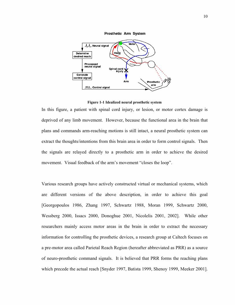
by thinking where to reach. Figure 1.1 illustrates an idealized prosthetic system to
command arm-reaching motions.
10
Figure 1-1 Idealized neural prosthetic system
In this figure, a patient with spinal cord injury, or lesion, or motor cortex damage is
deprived of any limb movement. However, because the functional area in the brain that
plans and commands arm-reaching motions is still intact, a neural prosthetic system can
extract the thoughts/intentions from this brain area in order to form control signals. Then
the signals are relayed directly to a prosthetic arm in order to achieve the desired
movement. Visual feedback of the arm’s movement “closes the loop”.
Various research groups have actively constructed virtual or mechanical systems, which
are different versions of the above description, in order to achieve this goal
[Georgopoulos 1986, Zhang 1997, Schwartz 1988, Moran 1999, Schwartz 2000,
Wessberg 2000, Issacs 2000, Donoghue 2001, Nicolelis 2001, 2002]. While other
researchers mainly access motor areas in the brain in order to extract the necessary
information for controlling the prosthetic devices, a research group at Caltech focuses on
a pre-motor area called Parietal Reach Region (hereafter abbreviated as PRR) as a source
of neuro-prosthetic command signals. It is believed that PRR forms the reaching plans
which precede the actual reach [Snyder 1997, Batista 1999, Shenoy 1999, Meeker 2001].

11
The advantage of using such high-level cognitive brain activities is that they are more
anatomically removed from regions that are damaged. While motor areas on the other
hand may degenerate following spinal cord injury [Florence 1998, Kaas 2002], most
cognitive areas of the brain are known to sustain even after loss of motor functions.
Furthermore, the plasticity, which is the capability of learning and adaptation, of the area
also holds promise that users may quickly learn to adapt to a brain machine interface
[Meeker 2003].
The construction of such a neuro-prosthetic system is no small feat. The quest of
designing and building the system involves disciplines ranging from neurobiology to
mechanical engineering, in which each field finds its interesting application or
challenging questions. Generally speaking, designing and building such a cognitively
controlled system requires several large building blocks: behavior experiments and signal
harvesting, learning and decoding machinery, control schemes, and system integration.
We briefly define each block and its function.
The behavioral experiments are controlled experiments in which the animal performs
designated behavior tasks while researchers monitor and record its brain activities. Then
either online or off-line, the recorded signals are examined to determine if any possible
patterns are embedded in the neural signals so that inferences can be made about the
animal’s behavioral states during the experiments. The procedure of inferring the
animal’s behaviors or sensory inputs from its recorded brain activities is termed
decoding. Next, knowledge gained in the learning/decoding stage enables us to construct

12
high-level control schemes necessary for commanding prosthetic devices so that they are
directed by the user’s thoughts. Finally, the software and hardware package must be
miniaturized for possible clinical implementation.
Among these building blocks, neural decoding is itself a very active research topic. It
includes, but is not limited to, characterizing the firing process of the spike trains and
estimating or predicting behavioral parameters from neural activities. A topic of ongoing
debate in the community is whether spike trains are rate coded or time coded: the former
refers to the assumption that the only informative feature in a spike train is the number of
spike counts observed in a time window, while the latter refers to the assumption that
timing between spike events also plays a role in conveying information. To answer this
question, different metrics and approaches ranging from statistical tools to information
theory have been proposed over the years [Teich 1986, Holt 1996, Koch 1997, Johnson
1996, Victor 1999, Johnson 2001]. In addition, the quest to promptly and accurately
predict some behavioral parameters from neural activities has also attracted large amount
of interest, especially in the emerging field of neural prosthetic systems [L. Abbot 1994,
Zhang 1997, Schwartz 1988, Moran 1999, Schwartz 2000, Wessberg 2000, Issacs 2000,
Nicolelis 2002].
In order to address the above questions, it is necessary to first understand the stochastic
characteristics of the spike train. In this thesis, a novel approach to characterize spike
trains is proposed. This approach determines the Poisson-ness of a spike train at different
scales. It takes advantage of the multi-scale capability of wavelet packets, a relatively

13
new signal processing technique. Under this approach, the spike trains are projected onto
wavelet packets and the distributions of the projection coefficients are analyzed. The
coefficients whose empirical distributions significantly deviate from the theoretical
distribution of a comparable Poisson process are counted. The higher the counts, the less
likely the process is Poisson in nature. It allows us to assess Poisson-ness from different
scales, thus avoiding the stationary assumptions employed in some other analysis of the
spike trains [Gabbinni and Koch 1998]. Both surrogate data and the spike data collected
from neurons in PRR are characterized using this approach.
With knowledge of a spike train’s underlying stochastic nature, it is natural to extend the
wavelet packet approach to the decoding problem described earlier. Most current
decoding efforts use the mean firing rate, i.e., the number of spikes in a window to
estimate the behavioral or stimulus parameters. When neurons are well characterized as a
Poisson process, this decoding model is appropriate. However, using the Haar wavelet
packet family, spike train features beyond mean firing rate can be exploited. In addition,
these features have biological interpretations that are appealing and intuitive to
researchers in the neuroscience community. Of all the features, the most informative
ones are the ones with the largest power to discriminate among the behavioral or stimulus
parameters; thus, decoding based on these features can potentially improve both accuracy
and efficiency. In this thesis I propose an optimal feature selection technique which
combines the wavelet packet framework with mutual information, an information
theoretic measure. Because of the hierarchical structure of the wavelet packet and the
special properties of the mutual information, this method returns the wavelet packet
14
projection coefficients with the largest decodability towards the decoding task. Finally, I
incorporate these selected features into a Bayesian classifier to estimate the behavioral
parameters, such as reach directions in the case of decoding from PRR. Again both
artificial data and actual neuronal data are used and the decoding performance is
compared against the ones using only mean firing rate.
Besides decoding the estimated reach directions from PRR signals, we must estimate
additional parameters from neural signals in order to successfully control a robotic device
using brain activities. These additional parameters are termed cognitive parameters in
this thesis. They describe the brain’s internal behavioral states. For a minimally
autonomous robotic device, we define the behavior states to include a baseline state,
reach planning states, and the reach execution go state. Because of the structure of the
postulated state transitions, we cast them into a novel framework. When combined with
an Interpreter that acts on the classification results of these states, it returns an efficient
algorithm that extracts the necessary control parameters. Experimental data collected
from animals performing a sequence of actions are subjected to this method while we
compare different state transition rules.
The contributions of this thesis work include the following:
• A novel wavelet based spike train characterization method that assesses the
underlying stochastic properties of given spike trains is introduced and studied.
Traditional characterization methods have limitations or shortcoming when
dealing with long term correlation or non-stationarity in the data. On the other

15
hand, because of the statistical properties of the Haar wavelet packet, this method
provides versatility and insight into the spike train’s characteristics compared to
the traditional approaches.
• A wavelet packet based feature extraction method that searches for the most
informative features in spike trains is introduced in this thesis. In many decoding
problems, researchers automatically use firing rate as the lone feature in their
decoding algorithms. Although for spike trains with Poisson nature, firing rate is
indeed the only informative feature, as shown in this thesis, not all spike trains
exhibit Poisson characteristics. Thus, more generally it is necessary to search for
features embedded in the spike trains that are most informative towards decoding.
The algorithm introduced here combines information theoretic measures with
wavelet packet tree pruning techniques and returns features that offer improved
decoding performance.
• Finally, this thesis offers a first look at decoding cognitive states from reach
movement sequences. For practical purposes, a neural prosthetic system requires
control signals beyond mere reach directions. Thus, this thesis presents a
framework based on finite state machine, and different transition rules are
explored. Although the framework is very simple, it is the first in the field that
demonstrates the feasibility of using cognitive parameters to control autonomous
prosthetic arm systems.
This thesis is organized as follows:
16
• Chapter 2 provides background information on the experimental paradigms used
to collect neural data, and introduces the data type used in this thesis. A brief
review of the wavelet and wavelet packet concepts, with a focus on Haar wavelet
family, is also presented in the chapter. And finally, we review the Bayesian
classifier, which is the principal estimation tool used in the thesis.
• Chapter 3 describes a method to characterize spike trains using the Haar wavelet
packet function. We investigate the probabilistic properties of the wavelet packet
projection coefficients of Poisson processes. From the analysis, we derive both
the analytical forms of the distribution and an iterative method that approximate
these distributions in practical situations. Additionally this chapter proposes a test
that investigates the Poisson-ness of an unknown spike processes. This chapter
concludes with applications of the test to different types of data.
• Chapter 4 presents a framework for decoding behavioral parameters from neural
activities. First we review mutual information as a measure that quantifies the
discriminability of each feature. Then we introduce an algorithm that uses the
mutual information as the decodability score and prunes the wavelet packet tree in
search of the best features for decoding. We compare the decoding performance
using the optimal features to the performance obtained when using just standard
firing rates with applications to surrogate data as well data from neurons in PRR.
In the appendix, we also present a finite sample analysis that further justifies the
use of mutual information.

17
• Chapter 5 presents work on decoding logic parameters and sequences of
behaviors. We define the necessary states and the state transition concepts that
enable a construction of an autonomous model. When coupled with an
Interpreter, this model allows us to integrate decoding with state transition rules
so that we can extract practical control signals for a prosthetic system. Several
different Interpreter rules are explored as we compare their performance to reach
sequences recorded from the animals.
Some final remarks as well as some future works are proposed in Chapter 6 to conclude
this thesis.
18
Chapter 2 Background This chapter provides background information on the experimental setup and the
mathematical model of the neural data used in the thesis. Also, brief overviews of
wavelet and wavelet packet are presented as well. Finally, we discuss relevant concepts
from Bayesian classification, which is the principal classification tool used through out
the thesis.
2.1 Experimental setup and data type
Most of the actual neuronal data used in this thesis are obtained from behavioral
experiments that were conducted on Rhesus monkeys (Macaca mulatta) performing
delayed center-out reach tasks, which are illustrated in Figure 2.1.
Baseline (500 ms)
Target (300 ms)
Plan (800 ms)
Completed (variable)
Go
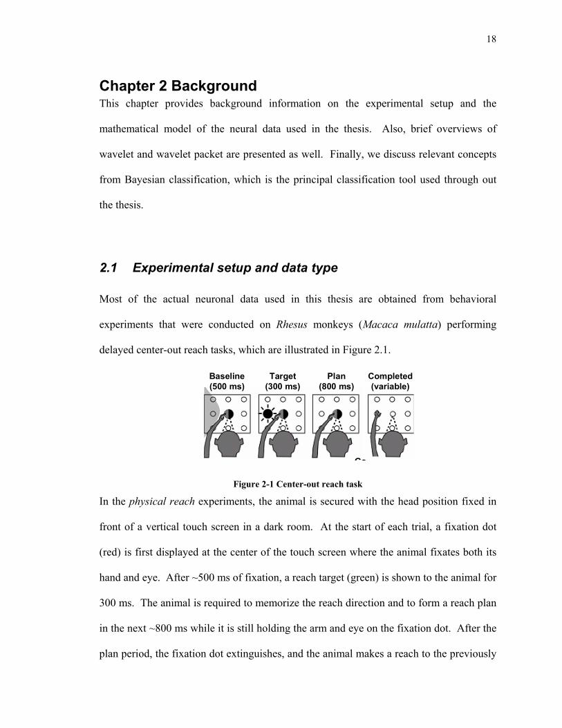
Figure 2-1 Center-out reach task
In the physical reach experiments, the animal is secured with the head position fixed in
front of a vertical touch screen in a dark room. At the start of each trial, a fixation dot
(red) is first displayed at the center of the touch screen where the animal fixates both its
hand and eye. After ~500 ms of fixation, a reach target (green) is shown to the animal for
300 ms. The animal is required to memorize the reach direction and to form a reach plan
in the next ~800 ms while it is still holding the arm and eye on the fixation dot. After the
plan period, the fixation dot extinguishes, and the animal makes a reach to the previously

19
shown target location. A juice reward is administered upon a successful completion of
the trial. The target locations are randomly chosen among 8 different locations, and the
length of the plan period is also randomized to minimize an anticipation effect [Batista
1999, Meeker 2001].
Alternatively, a virtual reach experiment very similar to the physical reach experiment is
carried out in order to simulate a neural prosthesis at work, and also to explore the
learning capability of PRR. The distinction between the physical reach and the virtual
reach is that in the latter, the animal does not actually perform the reach movement.
Instead of moving its arm towards the target, the animal forms the intention of making
the movement, which is subsequently decoded. Based on the decoded reach direction, a
visual feedback (yellow dot) appears on the touch screen. The animal is given the juice
award if the decoded reach direction matches the target.
The recording apparatus consists of a custom-made micro-electrode, signal amplifier,
A/D converter, and spike detection and sorting software. The micro-electrode is a 10 cm
long glass-coated platinum-iridium wire with the diameter 0.4 mm. The wire is insulated
throughout except at the sharpened tip, thus giving it an impedance of 1.5-2 MOhm. The
wire is housed in a glass guide tube of diameter 0.5 mm so that it can penetrate the dura
upon insertion. The A/D converter has a sampling frequency for 40 KHz for the brain
activities.
20
During a recording session, the electrode is first acutely inserted into the brain’s
functional area pre-determined using fMRI. Then using a micro-drive, the electrode is
advanced incrementally at 700 microns per step in the vicinity of PRR in searching for
extra-cellular neuronal activities. Once extra-cellular activities are detected, the animal is
required to make a sequence of movements to the 8 different locations in order to decide
the relevance of the neuron with respect to the behavior paradigm. If no identifiable
correlation exists between the neural activity and the reach locations, the electrode is
advanced further until new extra-cellular activities are detected; otherwise, the electrode
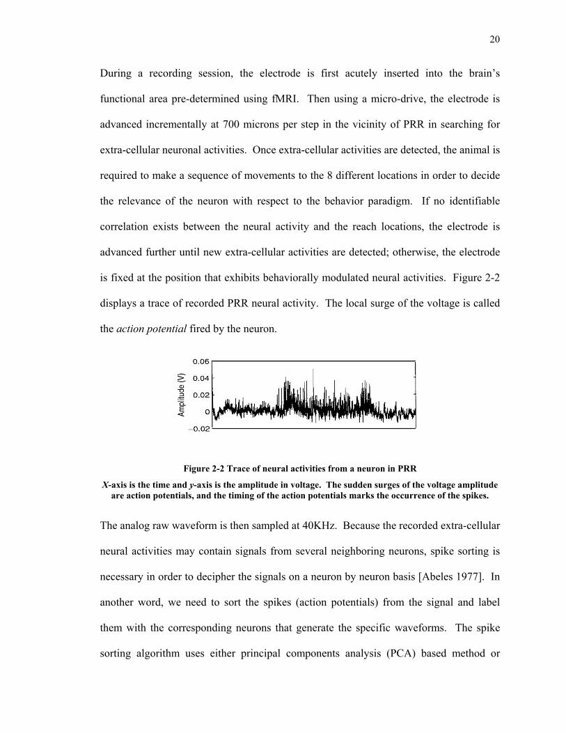
is fixed at the position that exhibits behaviorally modulated neural activities. Figure 2-2
displays a trace of recorded PRR neural activity. The local surge of the voltage is called
the action potential fired by the neuron.
Figure 2-2 Trace of neural activities from a neuron in PRR
X-axis is the time and y-axis is the amplitude in voltage. The sudden surges of the voltage amplitude are action potentials, and the timing of the action potentials marks the occurrence of the spikes.
The analog raw waveform is then sampled at 40KHz. Because the recorded extra-cellular
neural activities may contain signals from several neighboring neurons, spike sorting is
necessary in order to decipher the signals on a neuron by neuron basis [Abeles 1977]. In
another word, we need to sort the spikes (action potentials) from the signal and label
them with the corresponding neurons that generate the specific waveforms. The spike
sorting algorithm uses either principal components analysis (PCA) based method or

21
template method [Lewicki 1998]. Once the spikes are sorted, the time of occurrence of
each spike is recorded to a precision of 1ms. A sequence of the spikes forms a spike
train, which is one of the most frequently used data types in the neuroscience community.
This thesis thus places a strong emphasis on the spike train data format though some of
the techniques described have broader applications. The model of the spike train will be
the topic of next section.
All of the experimental neural signals used in this thesis are recorded from the Parietal
Reach Region (PRR), a sub-region of Posterior Parietal Cortex. PRR is believed to be
responsible for reach intentions or planning. A series of papers on this area suggest that
it not only encodes the reach plan in the retinotopic coordinates, but also codes the next
movement target in a sequential reach task [Snyder 1997, Batista 1999]. Therefore,
unlike motor areas, PRR encodes relatively simple movement parameters in a
straightforward coordinate frame. In addition, the posterior parietal cortex bridges the
sensory-motor transformation areas, which may be important for the type of learning
necessary for the proper alignment of sensory maps with motor maps, as demonstrated in
some recent works [Meeker 2003]. The learning ability of the area is especially
appealing for neural prosthetic applications because PRR may retain or quickly re-
establish the reach planning ability. Taking advantage of its learning ability thus may
prove necessary for optimizing the performance of a neural prosthesis.
22
2.2 Spike train representation
In the previous section, a brief description on the data collection apparatus is introduced.
The over-sampled analytical signals as seen in Figure 2.2 are further processed to
generate spike trains. The two basic pre-processing steps are spike detection and spike
sorting. The spike detection step separates the action potentials from background noises
such as thermal noise of the recording equipment and the average response from
neighboring neurons. There are many detection methods in existence, and the one
applied in this thesis is the thresholding method [Humphrey 1979, Abels and Goldstein
1977, Nenadic 2003]. It indicates the presence of a spike when a local peak of the raw
analytical signal passes a threshold. As a stream of spikes is recorded, the next step is to
classify the spikes to their respective source neurons because not all observed spikes are
originated by the same neuron. Many times two or three neighboring neurons may be
responsible for some of the spikes. The spike sorting technique used in this thesis is the
template method [Lewicki 1998]. Because the spike waveforms (128 data points of the
raw data centered around a peak) are markedly different given different neurons while
remaining homogeneous for the same neuron, the template method matches different
templates to all the observed spike waveforms. The ones exhibit similarities are
classified as being from the same neuron; and vice versa. Thus, the raw analytical signal
is deciphered into several data streams, each with spikes believed to be generated from
different neurons. In addition, because the spike waveforms for a given neuron are very
homogeneous, only the timings of the spikes are retained [Rieke 1997]. Finally, because
the refractory period physically limits a neuron’s ability to fire consecutive spikes within
23
2 ms, the processed and sort signals are down sampled to 1 kHz. This processed version
of the spike will be used throughout this thesis.
We employ a standard representation of a spike train as a binary function with 0’s and
1’s. We assume that the onset of a spike can be localized at best to a sampling interval of
length δT. Moreover, we assume that spikes are sampled over an interval of length T,
where T=2mδT for some integer m. With this assumption, a spike train, s, can be
described as
Equation 2.1
+=+=
=,])1(,[0,])1(,[1
)(kk
kk
IinspikenoisthereifTkTkIinIinspikeaisthereifTkTkIin
tsδδδδ
.
Equivalently, a spike train can be interpreted as a T-dimensional vector (where T=2m for
some integer m), whose kth element is determined as
Equation 2.2 +=
=otherwise
TkTkIinspikeaexiststhereifs k
k 0])1(,[1 δδ
,
where k=0,…,T-1. For some analyses, we further assume that there exists an ensemble of
N spike trains gathered under repeated behavioral, stimulus, and recording conditions.
Conceptually, these different spike trains are different samples of the same underlying
stochastic process. A superscript will index the members of the ensemble: { } Mits ,..,1)( = . In
all the computational examples of this paper, the sampling interval δT is taken to be 1ms
because of the refractory period. It is the physiological limit on the time intervals
between two consecutive spikes fired by the same neuron. Generally the refractory
period is taken to be 2ms, meaning a neuron can not fire a spike within the 2ms following
an earlier firing [Rieke 1997].
24
2.3 Haar Wavelet Packet Projection
We now review the Haar wavelet packet, its waveform, and its construction. Details are
outlined in several standard textbooks on wavelet theory [Daubechies 1992, Wickhauser
1994, Mallat 1999, Percival and Walden 2000]. This section also establishes our notation
for the projection coefficients of the spike trains. Knowledgeable reader may skip this
section and proceed directly to Section 2.4.
2.3.1 Haar Wavelet Review
A wavelet basis is a set of orthonormal functions that partition the time-frequency
domain in a dyadic fashion. As shown below, wavelets are constructed from a choice of
scaling function and a set of filters. In one sense, a filter can be interpreted as a set of
coefficients that are applied to a data stream in order to reveal meaningful features. That
is, let a filter be defined by a set of coefficients, {hk}, k=1,..,L. The filter output is given
by
∑ +=k
kiki xhv ,
where xk represents the raw data stream, the hk’s are the filter coefficients, and vi is the
filter output, or feature. From another perspective, filters are usually described by their
frequency domain characteristics because the filtering operation resembles convolution,
which is equivalent to multiplication in the frequency domain [Oppenheim 1999]. Some
basic types of filters include low pass (attenuates high frequency) and high pass
(attenuates low frequency). In this section we describe a filter by its filter coefficients.

25
We begin with the continuous wavelet function. First we define a low pass filter H by
coefficients { }kh and a complementary high pass filter G by coefficients { }kg , where the
coefficients { }kg and { }kh are required to have the following relationship:
kLk
k hg −−= )1( , L being the number of filter coefficients. These filters are generally
termed Quadrature Mirror Filters (QMF) [Percival 2001]. Next define a scaling function,
)(tφ , that satisfies the following conditions,
Equation 2.3 ∫∑∞
∞−=
=−= 1)(,)2(2)(1
dttkthtL
kk φφφ .
For simplicity, we denote the analogous operations of convolution and scaling by a factor
of two (“decimation”) with respect to the filter pair { }kh and { }kg by H and G, i.e.,
∑∑ −=−=k
kk
k ktfgGfktfhHf )2()2( .
Now construct a function, )(tψ , complimentary to )(tφ , such that
Equation 2.4 ∫∑ =−=Rk
k dttktgt 0)()2(2)( ψφψ ,
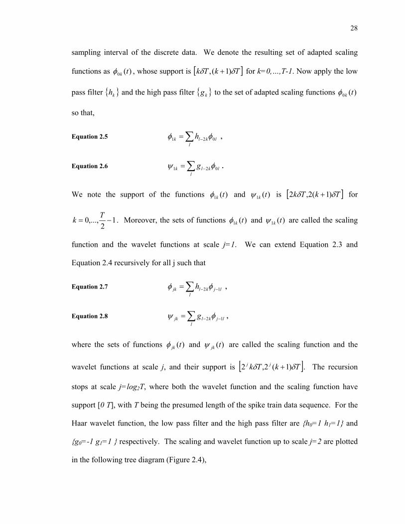
where )(tψ is termed the wavelet function. For the Haar wavelet function, the low pass
filter and the high pass filter coefficients are {1 1} and {-1 1}, respectively. The
associated scaling function and wavelet functions are plotted in Figure 2.3.

26
0 0.2 0.4 0.6 0.8 10
0.5
1
1.5
2
Haar scaling function
0 0.2 0.4 0.6 0.8 1-2
-1
0
1
2
Haar wavelet function
Figure 2-3 Haar scaling function and Haar wavelet Function on the interval [0 1].
X-axis is the time in ms and y-axis is the value of the functions.
The strength of wavelet-based analysis for this application resides in both its multi-
resolution analysis (MRA) capability and the computational efficiency of the associated
numerical algorithms. To understand MRA, consider a nested sequence of subspaces
{ }ZjjV
∈ of )(2 RL , where Z is the set of integers and )(2 RL is the space of all square
integrable functions. These nested subspaces satisfy the following conditions:
C1 211 LVVV jjj ⊂⊂⊂⊂⊂ +− LL for all Zj ∈ ,
C2 2lim LV jj=
∞→,
C3 }0{lim =−∞→ jj
V .
Further, define another complementary set of subspaces { }ZjjW
∈ such that
jjj WVV ⊕=+1 .
27
Combining the above definitions, the space )(2 RL can be expressed as
jjWRL
∞
−∞=⊕=)(2 .
This relation is termed a Multi-Resolution Analysis [Mallat 1999]. Using the actions of
translation and dilation, one can construct the following indexed version of the wavelet
function, )(tψ ,
)2(2)( 2/, ktt jjkj −= ψψ ,
where j is the scale (or dilation) index and k is the location (or translation) index.
Because for a fixed integer j*, the set of functions { },....1|)(,* =ktkj
ψ forms a basis for the
subspace *jW , the set of functions { },...1,...;1|)(, == kjtkjψ forms a basis for )(2 RL
with different resolutions indexed by j [Percival 2001]. Hence any signal )()( 2 RLtf ∈
can be represented as a weighted sum of the wavelet bases:
)()( ,,tvtf kjkj jk ψ∑= ,
where the weighting coefficients jkv are obtained by projection onto the wavelet basis via
the regular inner product on )(2 RL ,
dtttfv kjjk ∫= )()( ,ψ .
Even though the MRA is defined for the continuous function space, )(2 RL , its
construction can be easily generalized to the domain of discrete data. Consider a vector X
in RT, the space of all T-dimensional vectors, where T =2m with m an integer. We can
interpret X as a discrete sampling of a continuous function at sampling interval δT. With
this interpretation in mind, the scaling function )(tφ is scaled and adapted to each
28
sampling interval of the discrete data. We denote the resulting set of adapted scaling
functions as )(0 tkφ , whose support is [ ]TkTk δδ )1(, + for k=0,…,T-1. Now apply the low
pass filter { }kh and the high pass filter { }kg to the set of adapted scaling functions )(0 tkφ
so that,
Equation 2.5 ∑ −=l
lklk h 021 φφ ,
Equation 2.6 ∑ −=l
lklk g 021 φψ .
We note the support of the functions )(1 tkφ and )(1 tkψ is [ ]TkTk δδ )1(2,2 + for
12
,...,0 −=Tk . Moreover, the sets of functions )(1 tkφ and )(1 tkψ are called the scaling
function and the wavelet functions at scale j=1. We can extend Equation 2.3 and
Equation 2.4 recursively for all j such that
Equation 2.7 ∑ −−=l
ljkljk h 12 φφ ,
Equation 2.8 ∑ −−=l
ljkljk g 12 φψ ,
where the sets of functions )(tjkφ and )(tjkψ are called the scaling function and the
wavelet functions at scale j, and their support is [ ]TkTk jj δδ )1(2,2 + . The recursion
stops at scale j=log2T, where both the wavelet function and the scaling function have
support [0 T], with T being the presumed length of the spike train data sequence. For the
Haar wavelet function, the low pass filter and the high pass filter are {h0=1 h1=1} and
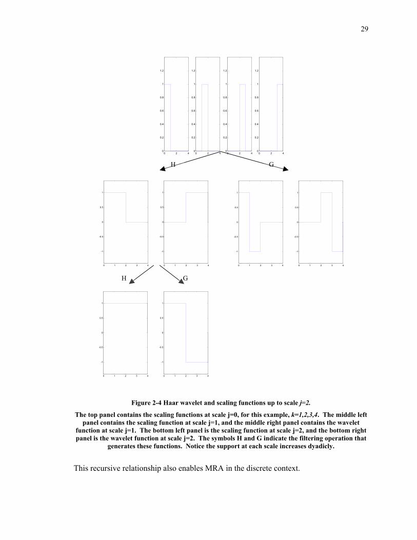
{g0=-1 g1=1 } respectively. The scaling and wavelet function up to scale j=2 are plotted
in the following tree diagram (Figure 2.4),
29
0 2 40
0.2
0.4
0.6
0.8
1
1.2
0 2 40
0.2
0.4
0.6
0.8
1
1.2
0 2 40
0.2
0.4
0.6
0.8
1
1.2
0 2 40
0.2
0.4
0.6
0.8
1
1.2
0 1 2 3 4
-1
-0.5
0
0.5
1
0 1 2 3 4
-1
-0.5
0
0.5
1
0 1 2 3 4
-1
-0.5
0
0.5
1
0 1 2 3 4
-1
-0.5
0
0.5
1
0 1 2 3 4
-1
-0.5
0
0.5
1
0 1 2 3 4
-1
-0.5
0
0.5
1
Figure 2-4 Haar wavelet and scaling functions up to scale j=2.
The top panel contains the scaling functions at scale j=0, for this example, k=1,2,3,4. The middle left panel contains the scaling function at scale j=1, and the middle right panel contains the wavelet
function at scale j=1. The bottom left panel is the scaling function at scale j=2, and the bottom right panel is the wavelet function at scale j=2. The symbols H and G indicate the filtering operation that
generates these functions. Notice the support at each scale increases dyadicly.
This recursive relationship also enables MRA in the discrete context.
H
H G
G
30
The above application of the wavelet functions to the discrete data inspires the so-called
Pyramid Algorithm [Mallat 1999], an efficient method for computing the wavelet
projection coefficients of discrete data. Again we take a vector X={x0,…,xT-1} in RT, the
space of all T-dimensional vectors, where T is a power of 2. Similarly, we interpret the
vector X as a piece-wise constant continuous function with constant values xk over the
sampling interval [ ]TkTk δδ )1(, + for k=0,…,T-1. The projection coefficients of X onto
the 0th scale scaling functions are,
∫= dtttXu kk )()( 00 φ .
Because X(t) is a piece-wise constant function with piecewise support coinciding with the
support of )(0 tkφ , and by Equation 2.3,
kk xu =0 .
Therefore, the finest scale coefficients are exactly the input data itself. Now we can use
the low pass filter { }kh and the high pass filter { }kg to recursively compute the wavelet
coefficients at each scale. The governing equations for the Pyramid Algorithm are
Equation 2.9 ∑ −−=l
ljkljk uhu ,12 ,
Equation 2.10 ∑ −−=l
ljkljk ugv ,12 ,
where the {vjk} are the wavelet projection coefficients and the {ujk} are the scaling
projection coefficients, an intermediate set of coefficients that are derived by projecting
the signal f(t) onto the scaling function )(tjkφ . In addition, the cardinality of the sets {vjk}
31
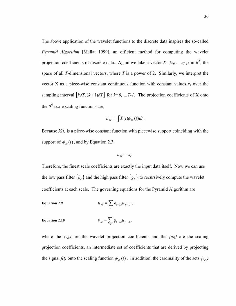
and {ujk} at each scale are j
T2
. For the Haar wavelet, we can illustrate the idea behind
the Pyramid algorithm using a decomposition tree similar to the one illustrated in Figure
2.4, where each node at level j in the tree represents a set of wavelet coefficients at scale
level j (Figure 2.5).
Figure 2-5 Pyramid Algorithm for the special case of Haar wavelet decomposition
At scale j=0, the scaling coefficients u0,k are the input data sequence whose length is T. At scale j = 1, we obtain the scaling coefficients u1,k and wavelet coefficients v1,k by performing the convolution-
decimation operation with H and G, respectively. Note the cardinality of the coefficient set is now T/2 because of the decimation. The two nodes at j=1 are termed children of the parent node at j=0
because they are derived from that parent node. Similarly, the scaling coefficients u2,k and wavelet coefficients v2,k at scale j=2 are generated from the parent node at scale j=1, and their corresponding
cardinality is T/4. Using this algorithm, we can proceed to calculate the wavelet coefficients at all scales until the size of the coefficient set equals 1.
2.3.2 Haar Wavelet Packet
The wavelet packet is an extension of the basic wavelet construction described above.
Because wavelet packets are a super-set of wavelets, they offer a richer selection of basis
functions. In the context of the spike train classification problem, this added richness
yields a more refined analysis of the spike train. The construction of the continuous Haar
wavelet packet basis functions again involves a low pass filter { } { }1,1=kh and a
complementary high pass filter { } { }1,1 −=kg . Assuming that the wavelet functions )(tψ
u0,k= s (spike train)
u1,k=u0,2k-1+u0,2k v1,k+T/2= u0,2k-1-u0,2k
u2,k v2,k
H
H
G
G
Scale j=0 k=0…T-1
Scale j=1 k=0…T/2-1
Scale j=2 k=0…T/4-1
32
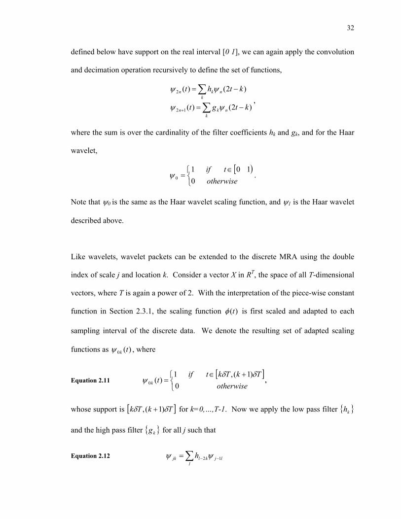
defined below have support on the real interval [0 1], we can again apply the convolution
and decimation operation recursively to define the set of functions,
∑
∑−=
−=
+k
nkn
knkn
ktgt
ktht
)2()(
)2()(
12
2
ψψ
ψψ,
where the sum is over the cardinality of the filter coefficients hk and gk, and for the Haar
wavelet,
[ ) ∈
=otherwise
tif0
1010ψ .
Note that ψ0 is the same as the Haar wavelet scaling function, and ψ1 is the Haar wavelet
described above.
Like wavelets, wavelet packets can be extended to the discrete MRA using the double
index of scale j and location k. Consider a vector X in RT, the space of all T-dimensional
vectors, where T is again a power of 2. With the interpretation of the piece-wise constant
function in Section 2.3.1, the scaling function )(tφ is first scaled and adapted to each
sampling interval of the discrete data. We denote the resulting set of adapted scaling
functions as )(0 tkψ , where
Equation 2.11 [ ]
+∈
=otherwise
TkTktiftk 0
)1(,1)(0
δδψ ,
whose support is [ ]TkTk δδ )1(, + for k=0,…,T-1. Now we apply the low pass filter { }kh
and the high pass filter { }kg for all j such that
Equation 2.12 ∑ −−=l
ljkljk h 12 ψψ

33
Equation 2.13 ∑ −−+
=l
ljklTjkg
j12
2
ψψ ,
where the sets of functions )(tjkψ have support [ ]TkTk jj δδ )1(2,2 + , and the limit of the
summation is the cardinality of the filter coefficients H and G. The recursion stops at
scale j=log2T, where both the wavelet packet functions have support [0 T]. For the Haar
wavelet function, the low pass filter and the high pass filter are {h0=1 h1=1} and {g0=-1
g1=1 } respectively, thus the relationship becomes
)()()( 2,112,1, ttt kjkjkj −−− += ψψψ , if low pass
)()()( 2,112,12
,ttt kjkjTkj j
−−−+
−= ψψψ , if high pass
where j is the scale index, k is the position index, and T is the length of support of the
filter at the largest scale, as defined above. An example of Haar wavelet packets and
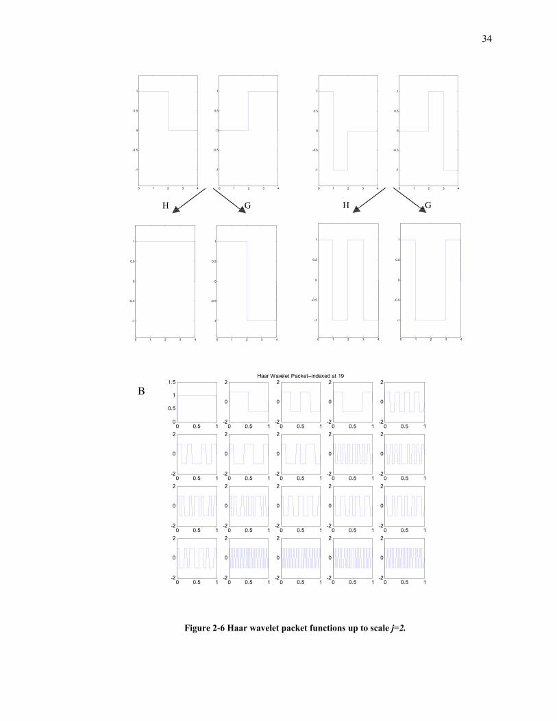
their recursion relationship is shown graphically in Figure 2-6.
0 2 40
0.2
0.4
0.6
0.8
1
1.2
0 2 40
0.2
0.4
0.6
0.8
1
1.2
0 2 40
0.2
0.4
0.6
0.8
1
1.2
0 2 40
0.2
0.4
0.6
0.8
1
1.2
H G
A
34
0 1 2 3 4
-1
-0.5
0
0.5
1
0 1 2 3 4
-1
-0.5
0
0.5
1
0 1 2 3 4
-1
-0.5
0
0.5
1
0 1 2 3 4
-1
-0.5
0
0.5
1
0 1 2 3 4
-1
-0.5
0
0.5
1
0 1 2 3 4
-1
-0.5
0
0.5
1
0 1 2 3 4
-1
-0.5
0
0.5
1
0 1 2 3 4
-1
-0.5
0
0.5
1
0 0.5 10
0.5
1
1.5
0 0.5 1-2
0
2
0 0.5 1-2
0
2Haar Wavelet Packet--indexed at 19
0 0.5 1-2
0
2
0 0.5 1-2
0
2
0 0.5 1-2
0
2
0 0.5 1-2
0
2
0 0.5 1-2
0
2
0 0.5 1-2
0
2
0 0.5 1-2
0
2
0 0.5 1-2
0
2
0 0.5 1-2
0
2
0 0.5 1-2
0
2
0 0.5 1-2
0
2
0 0.5 1-2
0
2
0 0.5 1-2
0
2
0 0.5 1-2
0
2
0 0.5 1-2
0
2
0 0.5 1-2
0
2
0 0.5 1-2
0
2
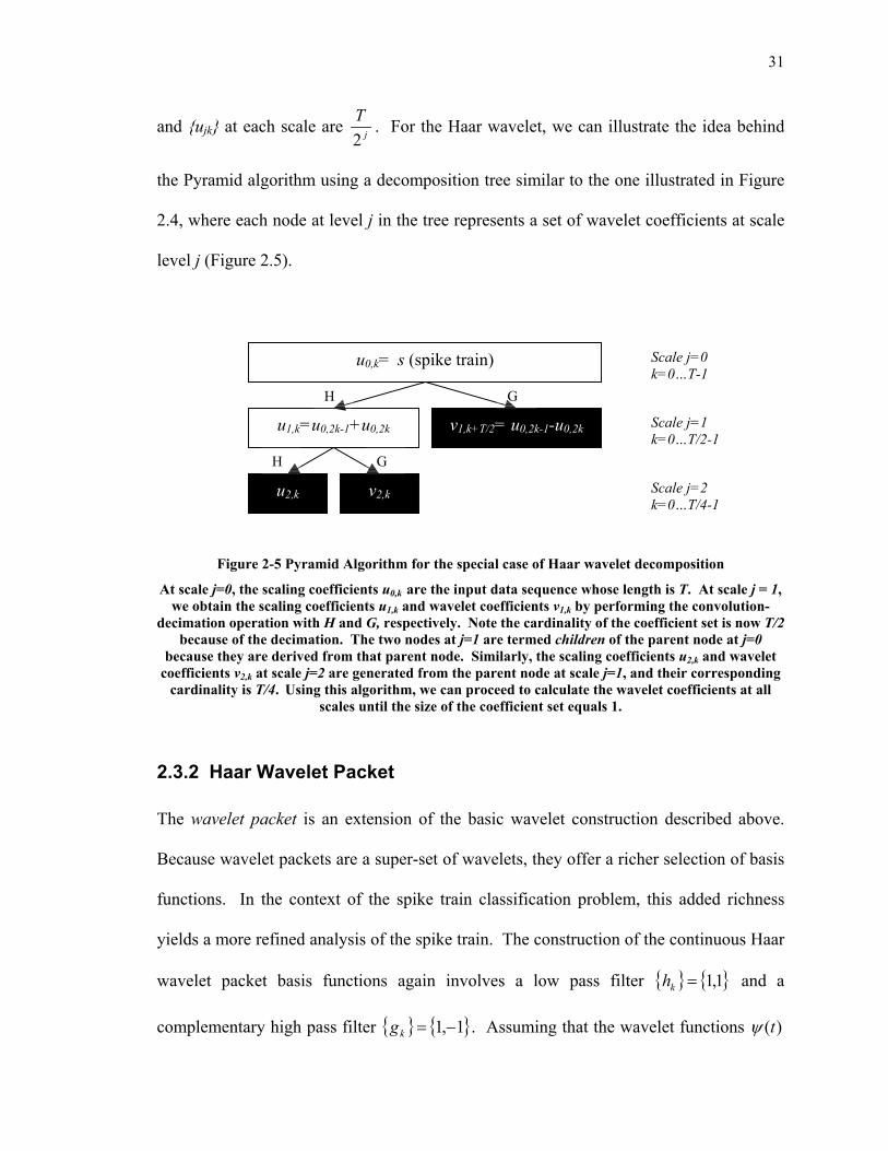
Figure 2-6 Haar wavelet packet functions up to scale j=2.
H G H G
B
35
A) The top panel contains the wavelet packet functions at scale j=0. It is identical to the scaling function. The middle left panels contain the wavelet packet functions at scale j=1 as a results of the low pass filtering, and the middle right panels contain ones as a results of high pass filtering. The
two bottom left panels contain the wavelet packet functions that are children of the two middle left ones, and similarly the two bottom right ones are children of the two middle right ones. The H and G
indicate the filtering operation towards these functions. Notice the support at each scale increases dyadicly. B) The Haar wavelet packet functions on [0 1] up to the 19th iteration.
In particular, we notice that the set of Haar wavelet functions is the left vertical branch in
the packet tree (Figure 2.6A).
An interesting property of the Haar wavelet packet functions is the orthogonal
relationship between all of the packet functions. Before describing the orthogonality in
detail, we first define several relevant terms. A tree is an arrangement of the wavelet
packet functions such that they are structured in a branching fashion. A node jlN is either
a tree branches or a tree leaf, and at a given scale j there are 2j nodes. In the above
example, there are 1 node N01 at scale j=0, 2 nodes at scale j=2, and 4 nodes at scale j=3.
Moreover, the member functions of a node are defined as the wavelet packet functions
related to each node. The relationship is the constructive iteration shown in Figure 2.6.
The number of member functions for any node at scale j is T/2j, where T is the length of
the input vector under investigation. Now we are in position to discuss the orthogonality
property.
Proposition 2.1 Member functions of each node are orthogonal to the member functions
of any nodes residing on a different branch of the dyadic tree.

36
For example, in the above figure, the member functions of N21 are orthogonal to the
members of N22, N23, and N24. Likewise, it is also orthogonal to the parent node of N23
and N24, namely N12 because N21 and N12 do not share a branch.
Proof:
Note that the member functions of any two child nodes derived from the same parent are
orthogonal. To show this, directly integrate the functions:
∫ dttt jkjk )()(21
ψψ ,
where )(1
tjkψ is a member function of 1jlN and )(
2tjkψ is a member function of
2jlN .
There are two possibilities for the above integration:
1) If jJkk −+≠
212 , then 0)()(21
=∫ dttt jkjk ψψ because by construction, 1jkψ and
2jkψ have
non-overlapping support.
2) If jJkk −+=
212 , then
0
)()(
)]()()][()([
)()(
22,1
212,1
2,112,12,112,1
11
1111
21
=
−=
−+=
−−−
−−−−−−
∫∫
∫
dttt
dttttt
dttt
kjkj
kjkjkjkj
jkjk
ψψ
ψψψψ
ψψ
.
In addition, the wavelet packet functions contained in the branches derived from the two
child nodes are also orthogonal. To see this, we observe that the space spanned by the
first child node is orthogonal to the one spanned by the second child, i.e.,
{ }11 jkSpanS ψ= , 11 nodechildk ∈
{ }22 jkSpanS ψ= , 22 nodechildk ∈
37
21 SS ⊥
because the member functions, { }1jkψ and { }
2jkψ are orthogonal as shown earlier.
Moreover, the wavelet packets contained in the branches of the two child nodes are linear
combinations of the ones in { }1jkψ and { }
2jkψ by construction. Hence they are also
orthogonal to one another.
Therefore, we have shown that the wavelet packet functions in any node are orthogonal
to the ones in nodes that are a member of a different branch. ٱ
Similarly, we can adopt the Pyramid Algorithm to efficiently compute the projection
coefficients of the wavelet packets. The algorithm is almost identical to the one used for
wavelets, with the only difference being that the branching of the wavelet packet tree
occurs at every node, while branching occurs only in the first node of its wavelet
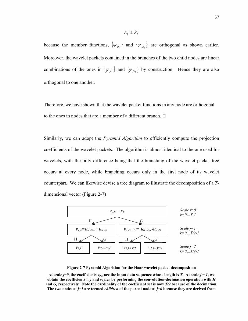
counterpart. We can likewise devise a tree diagram to illustrate the decomposition of a T-
dimensional vector (Figure 2-7)
Figure 2-7 Pyramid Algorithm for the Haar wavelet packet decomposition
At scale j=0, the coefficients v0,k are the input data sequence whose length is T. At scale j = 1, we obtain the coefficients v1,k and v1,k+T/2 by performing the convolution-decimation operation with H
and G, respectively. Note the cardinality of the coefficient set is now T/2 because of the decimation. The two nodes at j=1 are termed children of the parent node at j=0 because they are derived from
v0,k= xk
v1,k=u0,2k-1+u0,2k v1,k+T/2= u0,2k-1-u0,2k
v2,k v2,k+T/4
H
H
G
G
Scale j=0 k=0…T-1
Scale j=1 k=0…T/2-1
Scale j=2 k=0…T/4-1
v2,k+T/2 v2,k+3T/4
GH

38
that parent node. Similarly, the same relationship is observed at scale j=2, in which the cardinality of the coefficients in each node becomes T/4.
Using this version of the Pyramid Algorithm, we can efficiently compute all the wavelet
packet coefficients up to scale j=log2T. In all, the wavelet packet decomposition of a
vector of length T returns TlogT wavelet packet coefficients, compared to the T
coefficients by wavelet decomposition.
2.3.3 Computing the Projection Coefficients
Using the concepts and the background presented in the previous sections, the T-
dimensional spike train, s={s0,…,sT-1} can be projected onto the Haar wavelet packets
using the aforementioned Pyramid Algorithm.
Based on spike train model shown in Section 1, the 0th scale wavelet packet coefficients
v0,k are precisely the original spike train sk,
Equation 2.14 kk sv =0 .
For the Haar wavelet packet, the recursive relations for the remaining coefficients then
become
)()()( 2,112,1, tvtvtv kjkjkj −−− += , if low pass
)()()( 2,112,12
,tvtvtv kjkjTkj j
−−−+
−= , if high pass.
39
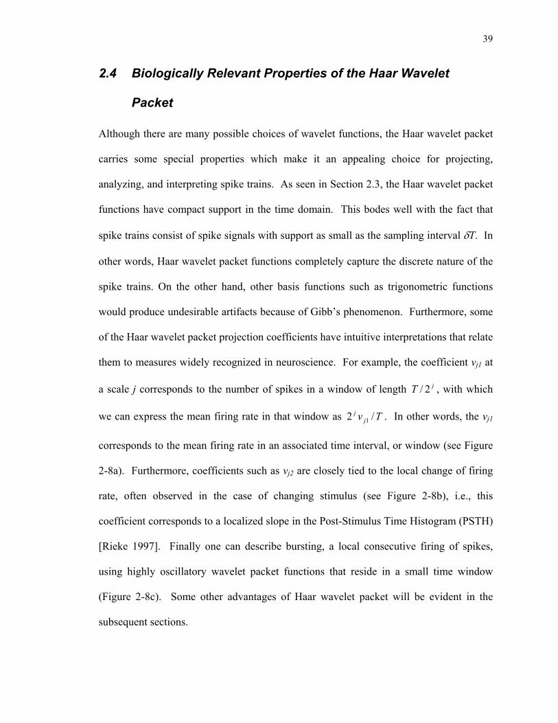
2.4 Biologically Relevant Properties of the Haar Wavelet
Packet
Although there are many possible choices of wavelet functions, the Haar wavelet packet
carries some special properties which make it an appealing choice for projecting,
analyzing, and interpreting spike trains. As seen in Section 2.3, the Haar wavelet packet
functions have compact support in the time domain. This bodes well with the fact that
spike trains consist of spike signals with support as small as the sampling interval δT. In
other words, Haar wavelet packet functions completely capture the discrete nature of the
spike trains. On the other hand, other basis functions such as trigonometric functions
would produce undesirable artifacts because of Gibb’s phenomenon. Furthermore, some
of the Haar wavelet packet projection coefficients have intuitive interpretations that relate
them to measures widely recognized in neuroscience. For example, the coefficient vj1 at
a scale j corresponds to the number of spikes in a window of length jT 2/ , with which
we can express the mean firing rate in that window as Tv jj /2 1 . In other words, the vj1
corresponds to the mean firing rate in an associated time interval, or window (see Figure
2-8a). Furthermore, coefficients such as vj2 are closely tied to the local change of firing
rate, often observed in the case of changing stimulus (see Figure 2-8b), i.e., this
coefficient corresponds to a localized slope in the Post-Stimulus Time Histogram (PSTH)
[Rieke 1997]. Finally one can describe bursting, a local consecutive firing of spikes,
using highly oscillatory wavelet packet functions that reside in a small time window
(Figure 2-8c). Some other advantages of Haar wavelet packet will be evident in the
subsequent sections.
40
0 50 100 150 200 250 300 350 400 450 500-2
-1
0
1
2
A
0 50 100 150 200 250 300 350 400 450 500-2
-1
0
1
2
B
0 50 100 150 200 250 300 350 400 450 500-2
-1
0
1
2
C
Figure 2-8 Haar wavelet packet function at different scale and locations over 512 units of the basic sampling period δT
A. j=9, k=1, the wavelet packet function corresponds to a window that spans the whole 512 units. Consequentially, the resulting coefficient v9,1 correlates to the mean firing rate in the sampling
window of length 512 δT. B. j=6, k = 10, the wavelet packet function corresponds to one up-down cycle over 64 units. The resulting coefficient v6,10 in this case represents the difference of the firing rate in two consecutive 32 units windows. C. j = 4, k =300, the wavelet packet function corresponds
to high frequency oscillation in a 16 units window. The resulting wavelet coefficients v4,300 have direct implication on local bursting activities.
2.5 Bayesian classifier
This section reviews basic concepts about the Bayesian classifier, a widely used
classification method. It classifies an unlabeled observation by estimating its probability
associated with each different class. More rigorously, denote the stimulus parameter
(class label) as X and the feature (unlabeled observation) as v, both are random variables.
Then the ubiquitous Bayes’ rule states that
Equation 2.15 )(
)()|()|(vP
XPXvPvXP = ,
41
where X is the class label, v is the feature, P(X|v) is the posterior probability, P(X) is the
prior probability of X, and P(v|X) is the likelihood of v given X. In this thesis X is
interpreted as the reach direction, and v as the neural signals. Bayesian classification is
based on the principle,
Equation 2.16 { })|(maxarg~
vXPXX
= ,
the estimated class or reach direction ~X is the one that maximizes the posterior
probability P(X|v).
Since the conditional probability p(v|X) must be estimated, this thesis estimates the
conditional densities using the Parzen window method [Parzen 1965]. The Parzen
window approach applies Gaussian kernels to the observed data and returns density
estimation in the form of the normalized sum of Gaussians centered at each data point.
We can write the resulting density function as
∑=
−==cN
ii
c
vvGN
cXvp1
),(1)|( σ ,
where G(v, σ) is a Gaussian kernel with standard deviation σ, and Nc is the total number
of trials in class Xc. Clearly p(v|X=c) is a density function because it integrates to 1 over
all values of v. Therefore, we can use the Parzen window approximation in place of the
true conditional density functions (which is unavailable) to estimate the mutual
information. The choice of σ controls the smoothness of the probability density.
42
A special case of the classification problems is the binary classification problem.
Because of its simplicity, many well-established theories of pattern recognition are built
upon the binary classification problem. Let the two classes be X1=1 and X2=0. The
Bayesian classification rule can be defined as
Equation 2.17 >=
=otherwise
vXPifxg
02/1)|1(1
)(* .
Interestingly this simple classification rule turns out be the optimal binary classifier.
Define the classification error E as
Equation 2.18 )()|~(
)~(
vPvXXP
XXPE
v∑ ≠=
≠=.
Theorem 2.1: [Devroye 1998] Let the Bayesian classification error be E*. That is, E* is
the error in the estimate produced by Equation 2.16, then EE ≤* for all E.
The above theorem shows that the Bayesian classifier minimizes the classification error
amongst all binary classifiers. This thesis thus uses Bayesian classifier as the principal
classification strategy.
43
Chapter 3 Characterizing spike train processes using Haar wavelet packet
3.1 Introduction
A sequence of spikes forms a spike train, which is often modeled as a random process [F.
Rieke 1997]. It is the most widely used data type in the neuroscience community.
Problems, such as neural encoding and decoding given spikes, have been studied
extensively [Gabbiani and Koch 1998, Rieke 1997, Victor 1997, Strong 1998, Johnson
1996, 2001]. However, the precise characteristics of this random process are still an open
question. Researchers have proposed different models to capture the statistical
characteristics of spike trains while the debate over the correctness of rate coding or
temporal coding of spike trains has been on going for some years [Johnson 1996, 2001,
Reich 2000, Steveninck, 2002]. Here rate coding refers to the assumption that
information is only conveyed in the firing rate of the spike train, and time coding refers to
the assumption that precise timing of the spikes also codes information. Schemes that
better characterize the firing process will help to understand the underlying neural code.
Often, the statistical behavior of a spike train is modeled as a homogeneous or
inhomogeneous Poisson process. A homogeneous Poisson process is completely
quantified by its mean firing rate, λ, which is equivalent to the number of spikes observed
in a fixed time period [Abbott 1994, Zhang 1998, Brown 1998]. Several approaches to
characterize a Poisson process have been proposed. The simplest approach is based on
counting the number of spikes in a window of length T, as the probability of observing n
spikes in the window is
44
( ) Tn
enTnp λλ −=!
)( .
Thus, for a homogeneous Poisson process the mean and variance of the spike counts up
to time T are both λT. The ratio of the variance to the mean is termed the Fano factor. A
unit value of this factor can indicate the presence of a Poisson process [Rieke 1997].
However, the Fano factor only focuses on the first two moments of a spike train’s
statistical characterization, while discarding the remaining higher ones. One can also
measure the coefficient of variation (COV), which is the ratio of the standard deviation to
the mean of the inter-spike intervals [Gabbiani and Koch 1998]. In the case of a Poisson
process, the COV is 1, which exemplifies one of the properties of a Poisson process: the
inter-spike intervals are exponentially distributed. However, using the COV as a measure
discards the possibility of discovering any possible patterns embedded in the spike trains
[Gabbiani and Koch 1998]. Another approach is to project the auto-correlation function
of a spike train onto a Fourier basis, and examine the resulting power spectral function
[Gabbiani and Koch 1998]. For a Poisson process, the power spectrum should be flat
everywhere except at the origin. Yet, the use of the auto-correlation function assumes by
default that the underlying spike generation process is stationary. When this assumption
is violated, blindly applying the power spectrum may produce artifacts in the frequency
domain [Mallat 1999]. The method described in this chapter can be applied to mildly
nonstationary signals.
This chapter introduces a new method to characterize spike trains based on wavelet
analysis. Particularly, it examines the projection of spike train ensembles onto a Haar
wavelet packet basis. If the spike generating process is stochastic by nature, the

45
coefficients obtained by projecting ensembles of the spike trains onto the wavelet packets
are random variables themselves. The statistical properties of the projection coefficients
shed light on the statistical nature of the spike train. This thesis shows that the
distribution of the projection coefficients for both homogeneous and inhomogeneous
Poisson processes can be well characterized. Using hypothesis testing on the coefficient
statistics, one can determine if a spike train is well characterized as a homogeneous or
inhomogeneous Poisson process. If the spike train is not deemed to be a Poisson process,
then this method also suggests the degree of non-Poisson-ness, and also highlights the
spike train’s characteristic time scales at which the spike train exhibits non-Poisson
behavior. To help visualize the degree of non-Poissonness at different scale, the Poisson
scale-gram is introduced. Taken together, these analyses provide guidance for further
investigations of a neural process in the case that it is significantly non-Poisson.
Furthermore, the characteristics of a spike train have important implications in the neural
decoding context. Decoding is the task of inferring external stimulus or behavioral
parameters given neural activities, or more precisely the spike trains in this thesis. If a
spike train is indeed Poisson by nature, then the stochastic properties of a Poisson process
suggests that mean firing rate is the only feature that carries information about the
stimulus parameter [Ross 1994], in which case decoding based on the mean firing rate
captures all the essential information content in the spike trains. On the other hand, if the
spike trains are not Poisson, then special treatment has to be applied in order to extract
the informative features embedded in the spike trains. Chapter 3 investigates the
decoding problem and the feature extraction approach in depth.
46
Generally, wavelet-based analysis is more suitable than Fourier analysis when dealing
with non-stationarity and specifically locally stationary processes [Mallat, 1998]. Power
spectrum based characterization method often encounters Gibbs phenomenon in which
local discontinuity of the signal produces bleeding of power into the higher frequency
domain, thus creating artifacts in the spectral-gram [Mallat 1999]. By using wavelet-
based methods, the spike train characterization technique presented here overcomes some
of the disadvantages of the methods reviewed above. Moreover, the multi-resolution
analysis feature of wavelets provides additional versatility in handling possible patterns
embedded in the spike trains. In this chapter, a wavelet basis consisting of the Haar
wavelet packet, which is an extension of the Haar wavelet [Wickerhauser 1994, Mallat
1999, Percival and Walden 2000], is the basis of the computational test. Some of the
Haar wavelet packet’s special properties, such as compactness and biologically intuitive
interpretations of the projection coefficients (see Section 2.2), make it an ideal candidate
for decomposing spike trains. Note that others have explored the possibility of using
wavelet packets as a mean of processing spike data [Kralik 2001, Oweiss 2001, 2002].
Yet, the work in this thesis appears to be the first to use wavelet methods for formal
characterization of spike trains.
This chapter is organized as follows. Section 2 analyzes the distribution of the wavelet
packet projection coefficients. Particular emphasis is placed on the special cases of
homogenous and inhomogeneous Poisson processes. In the case of the homogeneous
process, the probabilities of the projection coefficients are obtained analytically. Finally,

47
in Section 4 we integrate these ideas into a methodology that characterizes spike train
modeled as stochastic point processes. Several examples illustrate the main points in
Section 5.
3.2 Statistics of projection coefficients
Chapter 2 reviewed the concepts underlying the construction of Haar wavelet packets,
and introduced the projection coefficients arising from a binary spike train. This section
investigates the statistics of these coefficients when the given firing process is a
homogeneous or inhomogeneous Poisson process. Using a hypothesis testing
methodology based on a χ2-statistic applied to the coefficient distributions, one can then
check if a given spike train is statistically close to a Poisson process by comparing the
statistics of the projected data against the formulas derived below. This hypothesis
testing approach is developed in the next section.
3.2.1 Homogeneous Poisson Process
For simplicity, let us first analyze the case of a homogeneous Poisson process with a
constant firing rate λ. Poisson processes have three relevant properties:
P1. Each non-overlapping time increment of a Poisson process is independent and
identically distributed with the probability, P(.) of a spike occurring in the interval
[t,t+∆t] given by
tNNP ttt ∆≈=−∆+ λ)1( ,
where N(t) is the counting process that counts the number of spikes up to time t.
48
P2. When conditioned on a fixed number of spikes, a Poisson process uniformly
distributes all the spikes in a window of length T. We can formulate this
mathematically as
TtNttttP ∆
==∆+<< )1|''( ,
i.e. given that only 1 spike occurs somewhere in a window of length T, the
probability of observing that spike in a any interval of length t∆ is T
t∆ .
P3. The probability of observing n spikes in a window of length T given the firing rate
λ is
( ) Tn
enTnP λλ −=!
)( .
Now we derive the probability distributions of wavelet packet coefficients generated by
the projection of an ensemble of spike trains that arises from a homogeneous Poisson
process with fixed firing rate λ onto the Haar wavelet packet. First, notice that the
resulting projection coefficients are integer valued because the Haar wavelet packets are
functions that assume the value -1 and 1 only; and the spike trains are similarly binary
valued. Also, recall from Equation 2.2 that the integrals of wavelet packet functions at all
scales are 0. This symmetry of the wavelet packet, when coupled with property P2,
implies that when a single spike is projected onto the support of a wavelet packet
function, the probabilities of the resulting coefficient being 1 or -1 are the same, namely
½. Based on this observation, we can write the conditional probabilities of the projection
coefficients as follows: given N spikes in a window of length T,
=−=
nN
NnNvPN
21)|2( , Nn ,...,1,0=
49
where )|( NkvP = is the probability that coefficient v takes the integer value k when N
spikes occur in the support of the wavelet packet function associated with coefficient ν.
In addition, we can write
∑∑ ==NN
NPNvPNvPvP )()|(),()( ,
where P(N) is the probability of finding N spikes in the time interval of length T,
expressed by property P3. Thus, the probability of observing a projection coefficient of
integer value n is
Equation 3.1 TN
N
N
eN
TnNN
nvP λλ −∞
=∑
+
==
)!2(2/2
21)(
2
0
2
, if n is even
Equation 3.2 TN
N
N
eN
TnNN
nvP λλ −∞
=∑
+
+
==
)!2(21
2
21)(
2
0
2
, if n is odd.
The above analysis offers the theoretical distributions for wavelet packet coefficients that
result from an ensemble of spike trains arising from a given a homogeneous Poisson
process with constant firing rate λ. In practice, spike trains are sampled discretely. Let
the finest sampling resolution be δT. For such discretely sampled data, the probability
distributions given above become approximations that only work well when the finest
sampling period, δT, is sufficiently small as compared to the length of the sampling
window T. In other words, property P2 is approximated in practice because the
probability distribution of N spikes conditioned on N is only uniform when δT is
infinitesimally small, which is not possible in actual applications. To better understand
this subtlety, consider the simple case where two spikes are to be placed in a sampling
window that is subdivided into two sampling periods, 1t∆ and 2t∆ . If one spike is placed

50
in the interval 1t∆ with probability ½, then the second spike has to reside in 2t∆ with
probability 1. Therefore, we see that the approximation breaks down in this case. In the
next section, where the more general case of inhomogeneous Poisson processes are
considered, I propose a computational approach that approximates those probabilities so
that they are not susceptible to discretization errors. In addition, the computational
approach can be generalized to inhomogeneous Poisson processes. The theoretical
derivations of this section provide a standard against which we can check our
computational theory in the simple case of a purely homogeneous Poisson process.
3.2.2 Inhomogeneous Poisson Process
An inhomogeneous Poisson process is a Poisson process with a variable firing rate λ(t).
Even though it’s not stationary like a homogeneous Poisson process, it retains the same
memoryless property, P2, namely that disjoint increments of an inhomogeneous Poisson
process are independent.
Due to the variable firing rate, the approach outlined in the previous section becomes
unfeasible for inhomogeneous Poisson processes because the probability of observing n
spikes in an interval of duration T is now a combinatorial problem that depends on the
cardinality of the different firing rates present in this interval. Fortunately, a simpler
alternative to the computation of the coefficient distributions exists by utilizing the
Pyramid Algorithm and the memory-less property of an inhomogeneous Poisson process.
Recall that an inhomogeneous Poisson process has independent disjoint increments, i.e.,
)()(),( 1,0,01,0,0 ++ = kkkk vPvPvvP ,
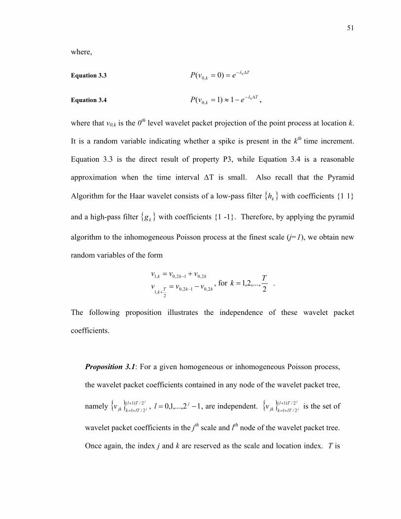
51
where,
Equation 3.3 Tk
kevP ∆−== λ)0( ,0
Equation 3.4 Tk
kevP ∆−−≈= λ1)1( ,0 ,
where that v0,k is the 0th level wavelet packet projection of the point process at location k.
It is a random variable indicating whether a spike is present in the kth time increment.
Equation 3.3 is the direct result of property P3, while Equation 3.4 is a reasonable
approximation when the time interval ∆T is small. Also recall that the Pyramid
Algorithm for the Haar wavelet consists of a low-pass filter { }kh with coefficients {1 1}
and a high-pass filter { }kg with coefficients {1 -1}. Therefore, by applying the pyramid
algorithm to the inhomogeneous Poisson process at the finest scale (j=1), we obtain new
random variables of the form
kkTk
kkk
vvvvvv
2,012,02
,1
2,012,0,1
−=
+=
−+
−
, for 2
,...,2,1 Tk = .
The following proposition illustrates the independence of these wavelet packet
coefficients.
Proposition 3.1: For a given homogeneous or inhomogeneous Poisson process,
the wavelet packet coefficients contained in any node of the wavelet packet tree,
namely { } j
jTllTkjkv 2/)1(
2/1+
+=, 12,...,1,0 −= jl , are independent. { } j
jTllTkjkv 2/)1(
2/1+
+= is the set of
wavelet packet coefficients in the jth scale and lth node of the wavelet packet tree.
Once again, the index j and k are reserved as the scale and location index. T is

52
the length of the spike train in multiples of δt. And l indexes the nodes at a
particular scale.
The proof of this proposition can be found in Appendix 1.
Based on the structural independence established by Proposition 3.1, the respective
probabilities of the coefficients v1,j then become
Equation 3.5 ∑ −==−
nvk nvPnPvvP
kkv)()()(
2,012,0,1 if 2/Tk ≤
Equation 3.6 ∑ +==+−
nvk nvPnPvvP
kkkv)'()()'(
2,012,0,1 otherwise ,
which are the convolutions between the probabilities of the parent random variables v0,k
and v0,k+1, a consequence of the above proposition.
The above equations can be extended to the wavelet packet coefficients at any scale. For
consistency we keep the same notation. We define the random variable obtained through
the wavelet packet projection at scale j position k as jkv . Then by the Pyramid
Algorithm,
1',1',1, +−− += kjkjkj vvv , if jNk −2/ even
1',1',1, +−− −= kjkjkj vvv , if jNk −2/ odd
where x is the floor operation that takes x to its nearest integer from below, and k’
indexes the parent nodes of kth node. And the corresponding probabilities can be
described using the convolutions,
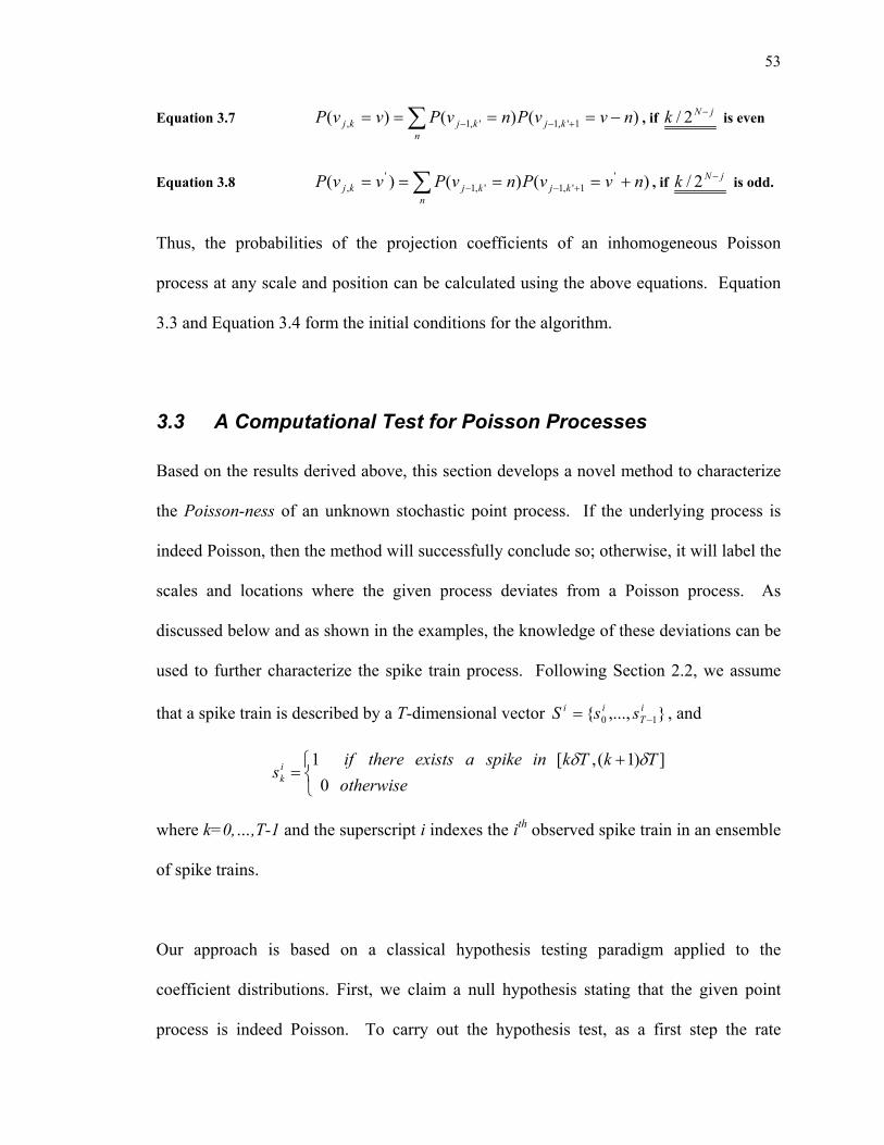
53
Equation 3.7 ∑ −==== +−−n
kjkjkj nvvPnvPvvP )()()( 1',1',1, , if jNk −2/ is even
Equation 3.8 ∑ +==== +−−n
kjkjkj nvvPnvPvvP )()()( '1',1',1
', , if jNk −2/ is odd.
Thus, the probabilities of the projection coefficients of an inhomogeneous Poisson
process at any scale and position can be calculated using the above equations. Equation
3.3 and Equation 3.4 form the initial conditions for the algorithm.
3.3 A Computational Test for Poisson Processes
Based on the results derived above, this section develops a novel method to characterize
the Poisson-ness of an unknown stochastic point process. If the underlying process is
indeed Poisson, then the method will successfully conclude so; otherwise, it will label the
scales and locations where the given process deviates from a Poisson process. As
discussed below and as shown in the examples, the knowledge of these deviations can be
used to further characterize the spike train process. Following Section 2.2, we assume
that a spike train is described by a T-dimensional vector },...,{ 10iT
ii ssS −= , and
+
=otherwise
TkTkinspikeaexiststhereifsi
k 0])1(,[1 δδ
where k=0,…,T-1 and the superscript i indexes the ith observed spike train in an ensemble
of spike trains.
Our approach is based on a classical hypothesis testing paradigm applied to the
coefficient distributions. First, we claim a null hypothesis stating that the given point
process is indeed Poisson. To carry out the hypothesis test, as a first step the rate

54
function λk, k=0,…,T-1 must be estimated from the spike train ensembles. Note that the
estimation of λ is itself an active research area [Donoho 1994, Kolaczyk 1997, Nowak
1999] This paper adopts the wavelet thresholding method proposed by Donoho to
estimate λ(t) from the spike trains. For completeness, the algorithm and its properties are
briefly reviewed. First we average the spike train ensemble over all the realizations i to
obtain a noisy estimation of the rate function at each time step k,
∑=
=L
i
ikk s
TM 1
1δ
λ
where L is the total number of spike trains of the ensemble. This computation effectively
estimates the firing rate at each sampling interval at length δT. Likewise, the standard
deviation of the rate function at each k can be estimated as
∑= −
−=
L
i
k
ik
k LT
s
1
2
1
][ λδσ .
Because of the Central Limit Theorem, kλ is asymptotically normally distributed for
each k when L approaches infinity. Therefore, we can scale the noisy rate function at
each time step by the quotient between L and the estimated standard deviation, σk, to
produce a scaled noisy rate function at each k,
kk
nsk
Lσ
λλ = ,
note that nskλ is normally distributed with variance 1 at each k again because of the
Central Limit Theorem. Now decompose the T-dimensional vector nskλ into wavelet
coefficients, αjk, using the Pyramid Algorithm described earlier

55
∑−
=
=1
0)(
T
l
dbjk
nsljk lψλα .
The family of wavelet functions, ψjk of choice here is Daubechie’s 4 wavelet (DB4)
[Percival 2001]. Note other wavelet built for de-noising also works in this context.
Following Donoho (1994), we threshold the wavelet coefficients using a threshold value
TT )log(2
=ε .
The thresholding rule is the so-called soft threshold, where the coefficients *jkα are
adjusted by the rule
>−
=otherwise
ifsign jkjkjkjk 0
)(* εαεααα .
Finally, we invert the thresholded wavelet coefficients to recover the de-noised rate
function λ={λk, k=0,…,T-1} using the following inversion formula:
∑=jk
dbjkjk t)(* ψαλ .
Certainly the robustness of the rate estimation process will affect any further analysis on
the Poisson nature of the spike train. However, as we will see below, the effect of rate
function estimation error vanishes exponentially with respect to the amount of data in this
characterization method.
Given the estimated rate function, the theoretical probabilities of each wavelet packet
coefficient can then be derived, i.e., the distribution of the projection coefficients under
the hypothesis that the process is an inhomogeneous Poisson process with rate function
λ(t) = {λk}, k=0,…,T-1. Again, because the rate function λ is a T-dimensional vector

56
with {λk}, k=0,…,T-1, the theoretical probabilities of the wavelet packet projection
coefficients are computed as
Tk
kevP δλ−== )0( ,0*
Tk
kevP δλ−−≈= 1)1( ,0*
and
∑ −==== +++n
kjkjkj nvvPnvPvvP )()()( 1',1*
',1*
,*
∑ +==== +++n
kjkjkj nvvPnvPvvP )()()( '1',1
*',1
*',
*
The notation P* represents the theoretical probability distribution given the spike
generation process is indeed Poisson with the above estimated firing rate function, λ(t).
Notice that the uncertainty associated with the seed probability P*(v0k) is
TkeP δελ )(* ±−≈∆ ,
where ε is proportional to the standard deviation of λk and to L/1 , the cardinality of the
ensemble. The error on the P* therefore is
TT eeE εδλδ m−= − 1 ,
which approaches 0 exponentially fast as the number of available data sets, L increases.
Hence, errors in the estimation error of λk have little effect on the estimated coefficient
probability distributions as L increases.
Meanwhile, one can also compute the respective empirical probabilities of all the wavelet
packet coefficients, P(vjk) from the data sets. Under the null hypothesis, the empirical
probabilities will match the hypothesized probabilities; otherwise, they will be
significantly different, indicating that the process is not Poisson. To assess the
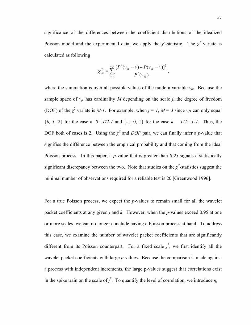
57
significance of the differences between the coefficient distributions of the idealized
Poisson model and the experimental data, we apply the χ2-statistic. The χ2 variate is
calculated as following
∑=
=−==
Mv
vv jk
jkjkjk vP
vvPvvP
1)(
)]()([*
2*2χ ,
where the summation is over all possible values of the random variable vjk. Because the
sample space of vjk has cardinality M depending on the scale j, the degree of freedom
(DOF) of the χ2 variate is M-1. For example, when j = 1, M = 3 since v1k can only equal
{0, 1, 2} for the case k=0…T/2-1 and {-1, 0, 1} for the case k = T/2…T-1. Thus, the
DOF both of cases is 2. Using the χ2 and DOF pair, we can finally infer a p-value that
signifies the difference between the empirical probability and that coming from the ideal
Poisson process. In this paper, a p-value that is greater than 0.95 signals a statistically
significant discrepancy between the two. Note that studies on the χ2-statistics suggest the
minimal number of observations required for a reliable test is 20 [Greenwood 1996].
For a true Poisson process, we expect the p-values to remain small for all the wavelet
packet coefficients at any given j and k. However, when the p-values exceed 0.95 at one
or more scales, we can no longer conclude having a Poisson process at hand. To address
this case, we examine the number of wavelet packet coefficients that are significantly
different from its Poisson counterpart. For a fixed scale j*, we first identify all the
wavelet packet coefficients with large p-values. Because the comparison is made against
a process with independent increments, the large p-values suggest that correlations exist
in the spike train on the scale of j*. To quantify the level of correlation, we introduce ηj

58
Equation 3.9 T
vvaluepv kjkjj
}95.0)(|{# **
*
>⋅=η ,
where T is the length of the spike train, i.e., the same as the number of wavelet packet
functions at a given scale. ηj marks the fraction of all the wavelet packet coefficients at
scale j that exhibits correlation. If ηj is small, then the correlation at that scale is minimal,
in which case we may label the process as approximately Poisson at that scale; else if ηj
is large, the process is deemed to be non-Poisson at that scale. When a given scale is
non-Poisson, it may be desirable to further investigate the dependence between the
wavelet packet coefficients residing in that scale in order to fully understand the spike
train process. In Section 3.4 we introduce the Poisson scale-gram as a simple graphical
technique to represent the non-Poissonness of a neural process.
3.4 Examples
To illustrate the utility of our approach, and to additionally show how the method can be
used to characterize spike trains, this section applies the methods described in the
previous sections to different data sets. In order to have a concrete understanding of the
ideas presented in Section 3.2, we first give an example of the coefficients’ distribution
when the underlying process is either a homogeneous or an inhomogeneous Poisson
process. Next we apply the spike characterization method outlined in Section 3.3 to a
number of different simulated and actual neural processes. The empirical distributions
throughout this section are computed using the histogram method.

59
Moreover the surrogate data used to produce the histograms in the simulation examples
below are generated using the following simple technique. For each 1ms window, we
compute the probability of not observing a spike as
001.0)0( kesP kλ−==
and observing a spike as
001.01)1( kesP kλ−−≈= .
Now we generate a uniform random number r using a generic random number generator.
If r>P(sk=0), we register a 1 at time k in the artificial spike train; otherwise, we register a
0 at time k. Thus, using this method we can generate spike trains of any given length that
model a Poisson process with rate function {λk}.
Example 1: The Coefficient Distributions of Poisson Processes
Before applying the characterizing method directly, we first study the distributions of the
projection coefficients in the case of idealized Poisson processes. As will be seen, the
nature of the coefficient distributions can shed light on the nature of the underlying
process. Consider the following three cases: 1) a homogeneous Poisson processes whose
constant firing rate is λ=20Hz; 2) an inhomogeneous Poisson process whose firing rate
function is a concatenation of two homogeneous Poisson processes, i.e., a Poisson
process with an abrupt change in firing rate
>≤
=2562025610
)(tt
tλ ;
and 3) an inhomogeneous Poisson process with a linear firing rate function
bmtt +=)(λ ,
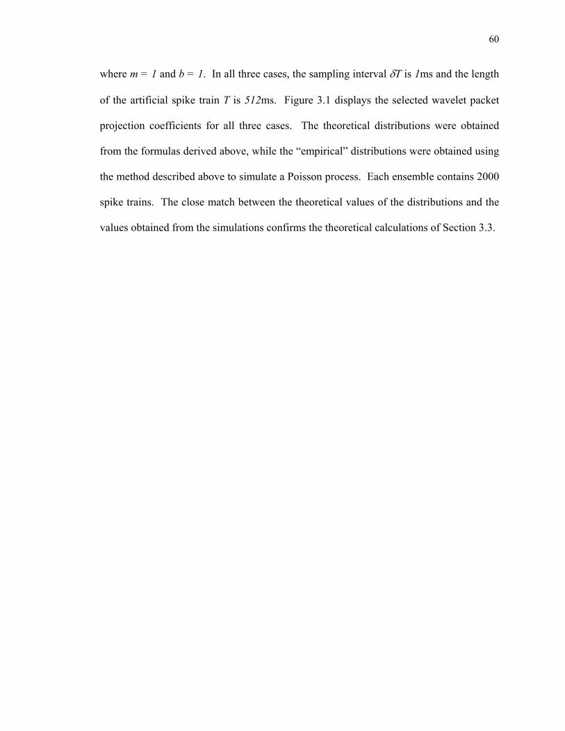
60
where m = 1 and b = 1. In all three cases, the sampling interval δT is 1ms and the length
of the artificial spike train T is 512ms. Figure 3.1 displays the selected wavelet packet
projection coefficients for all three cases. The theoretical distributions were obtained
from the formulas derived above, while the “empirical” distributions were obtained using
the method described above to simulate a Poisson process. Each ensemble contains 2000
spike trains. The close match between the theoretical values of the distributions and the
values obtained from the simulations confirms the theoretical calculations of Section 3.3.
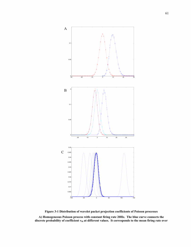
61
-30 -20 -10 0 10 20 300
0.05
0.1
-20 -10 0 10 20 30
0
0.05
0.1
0.15
-100 -50 0 50 100 1500
0.005
0.01
0.015
0.02
0.025
0.03
0.035
0.04
0.045
0.05
Figure 3-1 Distribution of wavelet packet projection coefficients of Poisson processes
A) Homogeneous Poisson process with constant firing rate 20Hz. The blue curve connects the discrete probability of coefficient v90 at different values. It corresponds to the mean firing rate over
A
B
C
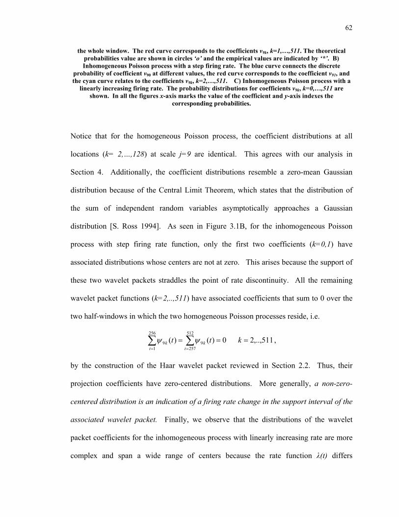
62
the whole window. The red curve corresponds to the coefficients v9k, k=1,…,511. The theoretical probabilities value are shown in circles ‘o’ and the empirical values are indicated by ‘*’. B) Inhomogeneous Poisson process with a step firing rate. The blue curve connects the discrete
probability of coefficient v90 at different values, the red curve corresponds to the coefficient v91, and the cyan curve relates to the coefficients v9k, k=2,…,511. C) Inhomogeneous Poisson process with a
linearly increasing firing rate. The probability distributions for coefficients v9k, k=0,…,511 are shown. In all the figures x-axis marks the value of the coefficient and y-axis indexes the
corresponding probabilities.
Notice that for the homogeneous Poisson process, the coefficient distributions at all
locations (k= 2,…,128) at scale j=9 are identical. This agrees with our analysis in
Section 4. Additionally, the coefficient distributions resemble a zero-mean Gaussian
distribution because of the Central Limit Theorem, which states that the distribution of
the sum of independent random variables asymptotically approaches a Gaussian
distribution [S. Ross 1994]. As seen in Figure 3.1B, for the inhomogeneous Poisson
process with step firing rate function, only the first two coefficients (k=0,1) have
associated distributions whose centers are not at zero. This arises because the support of
these two wavelet packets straddles the point of rate discontinuity. All the remaining
wavelet packet functions (k=2,..,511) have associated coefficients that sum to 0 over the
two half-windows in which the two homogeneous Poisson processes reside, i.e.
511,..,20)()(512
2579
256
19 === ∑∑
==
kttt
kt
k ψψ ,
by the construction of the Haar wavelet packet reviewed in Section 2.2. Thus, their
projection coefficients have zero-centered distributions. More generally, a non-zero-
centered distribution is an indication of a firing rate change in the support interval of the
associated wavelet packet. Finally, we observe that the distributions of the wavelet
packet coefficients for the inhomogeneous process with linearly increasing rate are more
complex and span a wide range of centers because the rate function λ(t) differs
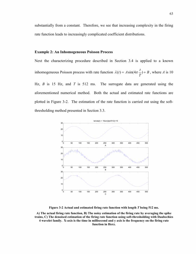
63
substantially from a constant. Therefore, we see that increasing complexity in the firing
rate function leads to increasingly complicated coefficient distributions.
Example 2: An Inhomogeneous Poisson Process
Next the characterizing procedure described in Section 3.4 is applied to a known
inhomogeneous Poisson process with rate function BTtAt += )4sin()( πλ , where A is 10
Hz, B is 15 Hz, and T is 512 ms. The surrogate data are generated using the
aforementioned numerical method. Both the actual and estimated rate functions are
plotted in Figure 3-2. The estimation of the rate function is carried out using the soft-
thresholding method presented in Section 3.3.
0 50 100 150 200 250 300 350 400 450 5000
10
20
30
A
lemda(t) = 10sin(4pit/512)+15
0 50 100 150 200 250 300 350 400 450 5000
10
20
30
B
0 50 100 150 200 250 300 350 400 450 5000
10
20
30
C
Figure 3-2 Actual and estimated firing rate function with length T being 512 ms.
A) The actual firing rate function, B) The noisy estimation of the firing rate by averaging the spike trains, C) The denoised estimation of the firing rate function using soft-thresholding with Daubechies
4 wavelet family. X-axis is the time in millisecond and y axis is the frequency on the firing rate function in Herz.
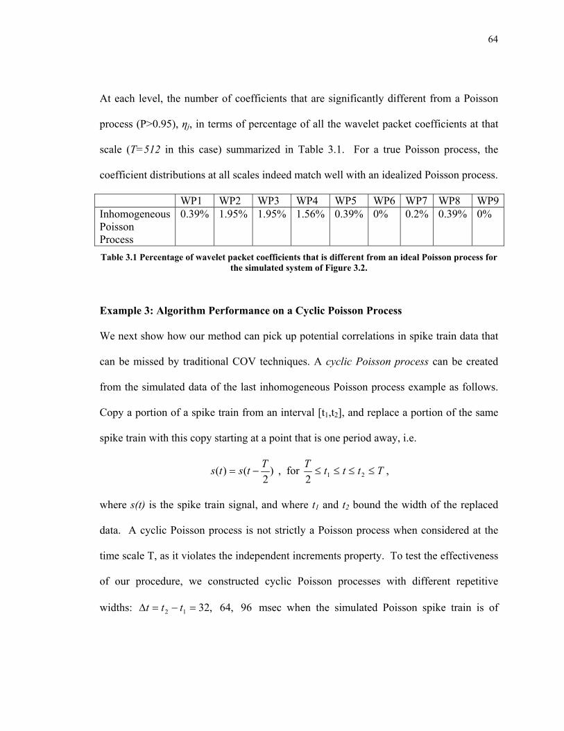
64
At each level, the number of coefficients that are significantly different from a Poisson
process (P>0.95), ηj, in terms of percentage of all the wavelet packet coefficients at that
scale (T=512 in this case) summarized in Table 3.1. For a true Poisson process, the
coefficient distributions at all scales indeed match well with an idealized Poisson process.
WP1 WP2 WP3 WP4 WP5 WP6 WP7 WP8 WP9Inhomogeneous Poisson Process
0.39% 1.95% 1.95% 1.56% 0.39% 0% 0.2% 0.39% 0%
Table 3.1 Percentage of wavelet packet coefficients that is different from an ideal Poisson process for the simulated system of Figure 3.2.
Example 3: Algorithm Performance on a Cyclic Poisson Process
We next show how our method can pick up potential correlations in spike train data that
can be missed by traditional COV techniques. A cyclic Poisson process can be created
from the simulated data of the last inhomogeneous Poisson process example as follows.
Copy a portion of a spike train from an interval [t1,t2], and replace a portion of the same
spike train with this copy starting at a point that is one period away, i.e.
)2
()( Ttsts −= , for TtttT≤≤≤≤ 212
,
where s(t) is the spike train signal, and where t1 and t2 bound the width of the replaced
data. A cyclic Poisson process is not strictly a Poisson process when considered at the
time scale T, as it violates the independent increments property. To test the effectiveness
of our procedure, we constructed cyclic Poisson processes with different repetitive
widths: 96,64,3212 =−=∆ ttt msec when the simulated Poisson spike train is of
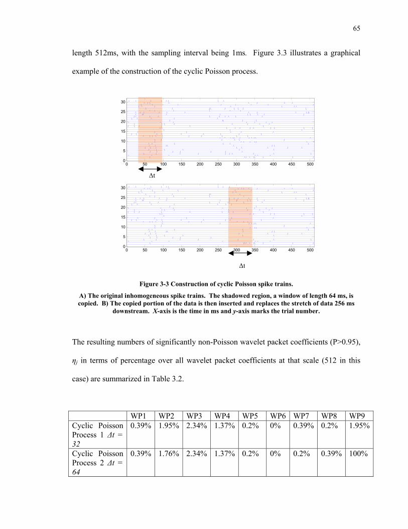
65
length 512ms, with the sampling interval being 1ms. Figure 3.3 illustrates a graphical
example of the construction of the cyclic Poisson process.
0 50 100 150 200 250 300 350 400 450 5000
5
10
15
20
25
30
0 50 100 150 200 250 300 350 400 450 5000
5
10
15
20
25
30
Figure 3-3 Construction of cyclic Poisson spike trains.
A) The original inhomogeneous spike trains. The shadowed region, a window of length 64 ms, is copied. B) The copied portion of the data is then inserted and replaces the stretch of data 256 ms
downstream. X-axis is the time in ms and y-axis marks the trial number.
The resulting numbers of significantly non-Poisson wavelet packet coefficients (P>0.95),
ηj in terms of percentage over all wavelet packet coefficients at that scale (512 in this
case) are summarized in Table 3.2.
WP1 WP2 WP3 WP4 WP5 WP6 WP7 WP8 WP9 Cyclic Poisson Process 1 ∆t = 32
0.39% 1.95% 2.34% 1.37% 0.2% 0% 0.39% 0.2% 1.95%
Cyclic Poisson Process 2 ∆t = 64
0.39% 1.76% 2.34% 1.37% 0.2% 0% 0.2% 0.39% 100%
∆t
∆t

66
Cyclic Poisson Process 3 ∆t = 96
0.39% 1.76% 2.34% 1.56% 0.2% 0% 0.78% 0.39% 100%
Table 3.2 Percentage of wavelet packet coefficients that are significantly different (P>0.95) from a Poisson process, η
For each scale j, the numbers of wavelet packet coefficients that are significantly different from the ones generated by a Poisson process are first counted, where the significance test is the proposed χ2 test. There are a total of 512 wavelet packet coefficients for each j, thus the percentage is calculated
as η=#{significant}/512.
Note that at scale j=9 (where the interval of support spans the entire 512 length cycle),
the number of significantly non-Poisson wavelet packet coefficients increases
dramatically as the length of the repetition window (the section of data copied and pasted)
∆t increases. An intuitive explanation is that the length of the repetition window is
proportional to the non-Poisson characteristics introduced in the process. In addition, ηj
at j=1,…,8 remains steadily small for all the experiments because all wavelet packet
functions at these scales have supports that are too short to simultaneously cover the two
identical stretches of data. Therefore, for scales j=1,…,8 the process appears Poisson
while at scale j=9, our method suggests that the data are not really Poisson due to the
correlations in the data that violate the independent increment assumption. On the other
hand, the COV analysis returns 1 for the cyclic Poisson processes because the repetition
in spike trains does not alter the inter-spike interval distribution.
Example 4: The Brandman and Nelson Non-renewal Model
We also apply the Poisson test to a known non-renewal process. Brandman and Nelson
(2002) proposed an adaptive linear threshold model neuronal firing model that generates
spike trains with non-renewal, specifically long-term regularization, properties. The
model has three parameters a, b, and σ, with a being proportional to the firing rate, and
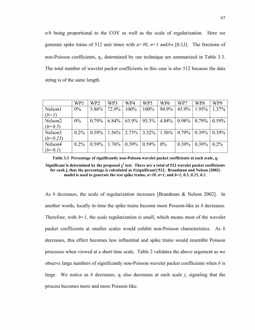
67
σ/b being proportional to the COV as well as the scale of regularization. Here we
generate spike trains of 512 unit times with a=30, σ=1 and ]1,1.0[∈b . The fractions of
non-Poisson coefficients, ηj, determined by our technique are summarized in Table 3.3.
The total number of wavelet packet coefficients in this case is also 512 because the data
string is of the same length.
WP1 WP2 WP3 WP4 WP5 WP6 WP7 WP8 WP9 Nelson1 (b=1)
0% 5.86% 72.9% 100% 100% 94.9% 45.9% 1.95% 1.37%
Nelson2 (b=0.5)
0% 0.79% 6.84% 63.9% 95.3% 4.88% 0.98% 0.79% 0.59%
Nelson3 (b=0.25)
0.2% 0.39% 1.56% 2.73% 3.32% 1.56% 0.79% 0.39% 0.39%
Nelson4 (b=0.1)
0.2% 0.59% 1.76% 0.39% 0.59% 0% 0.39% 0.39% 0.2%
Table 3.3 Percentage of significantly non-Poisson wavelet packet coefficients at each scale, ηj
Significant is determined by the proposed χ2 test. There are a total of 512 wavelet packet coefficients for each j, thus the percentage is calculated as #{significant}/512. Brandman and Nelson (2002)
model is used to generate the test spike trains; a=30, σ=1, and b=1, 0.5, 0.25, 0.1.
As b decreases, the scale of regularization increases [Brandman & Nelson 2002]. In
another words, locally in time the spike trains become more Poisson-like as b decreases.
Therefore, with b=1, the scale regularization is small, which means most of the wavelet
packet coefficients at smaller scales would exhibit non-Poisson characteristics. As b
decreases, this effect becomes less influential and spike trains would resemble Poisson
processes when viewed at a short time scale. Table 2 validates the above argument as we
observe large numbers of significantly non-Poisson wavelet packet coefficients when b is
large. We notice as b decreases, ηj also decreases at each scale j, signaling that the
process becomes more and more Poisson-like.
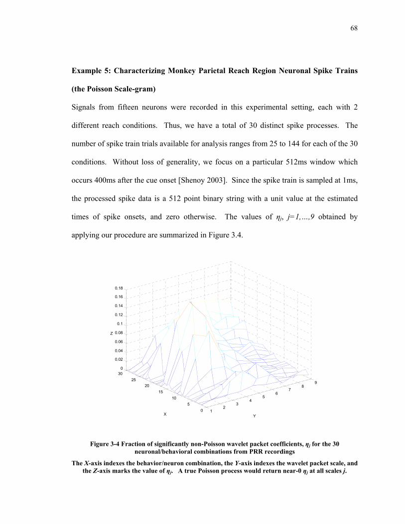
68
Example 5: Characterizing Monkey Parietal Reach Region Neuronal Spike Trains
(the Poisson Scale-gram)
Signals from fifteen neurons were recorded in this experimental setting, each with 2
different reach conditions. Thus, we have a total of 30 distinct spike processes. The
number of spike train trials available for analysis ranges from 25 to 144 for each of the 30
conditions. Without loss of generality, we focus on a particular 512ms window which
occurs 400ms after the cue onset [Shenoy 2003]. Since the spike train is sampled at 1ms,
the processed spike data is a 512 point binary string with a unit value at the estimated
times of spike onsets, and zero otherwise. The values of ηj, j=1,…,9 obtained by
applying our procedure are summarized in Figure 3.4.
12
34
56
78
9
05
1015
2025
300
0.02
0.04
0.06
0.08
0.1
0.12
0.14
0.16
0.18
YX
Z
Figure 3-4 Fraction of significantly non-Poisson wavelet packet coefficients, ηj for the 30 neuronal/behavioral combinations from PRR recordings
The X-axis indexes the behavior/neuron combination, the Y-axis indexes the wavelet packet scale, and the Z-axis marks the value of ηj. A true Poisson process would return near-0 ηj at all scales j.
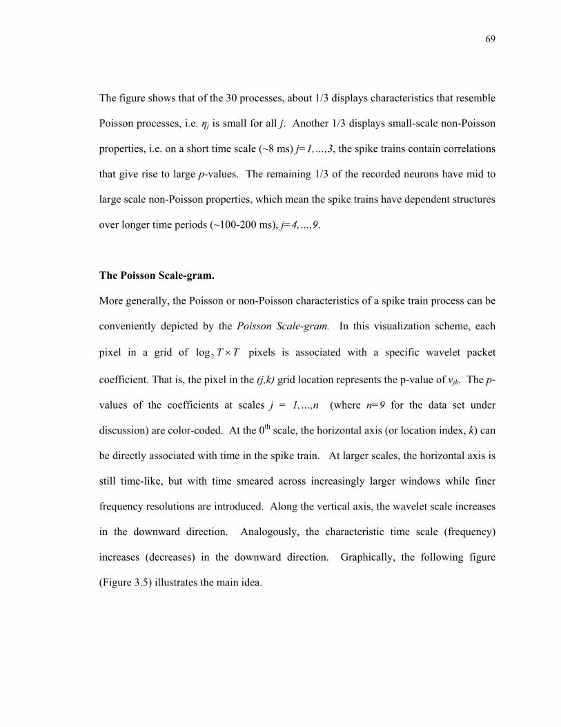
69
The figure shows that of the 30 processes, about 1/3 displays characteristics that resemble
Poisson processes, i.e. ηj is small for all j. Another 1/3 displays small-scale non-Poisson
properties, i.e. on a short time scale (~8 ms) j=1,…,3, the spike trains contain correlations
that give rise to large p-values. The remaining 1/3 of the recorded neurons have mid to
large scale non-Poisson properties, which mean the spike trains have dependent structures
over longer time periods (~100-200 ms), j=4,…,9.
The Poisson Scale-gram.
More generally, the Poisson or non-Poisson characteristics of a spike train process can be
conveniently depicted by the Poisson Scale-gram. In this visualization scheme, each
pixel in a grid of TT ×2log pixels is associated with a specific wavelet packet
coefficient. That is, the pixel in the (j,k) grid location represents the p-value of vjk. The p-
values of the coefficients at scales j = 1,…,n (where n=9 for the data set under
discussion) are color-coded. At the 0th scale, the horizontal axis (or location index, k) can
be directly associated with time in the spike train. At larger scales, the horizontal axis is
still time-like, but with time smeared across increasingly larger windows while finer
frequency resolutions are introduced. Along the vertical axis, the wavelet scale increases
in the downward direction. Analogously, the characteristic time scale (frequency)
increases (decreases) in the downward direction. Graphically, the following figure
(Figure 3.5) illustrates the main idea.

70
Figure 3.5 Illustration of the Poisson Scale-gram
Each pixel represents the p-value of the χ2 variate associated with the wavelet coefficient vjk. The scale j decreases from 1 to log2T, and the location k increases from 0 to T-1. There are a total of Tlog2T pixels in the image. At the smaller scales, the location index k is strongly related to time
increments. But at larger scales, the temporal resolution is traded off by the frequency resolution, as k indexes frequency increments.
We have chosen a color scale based on blue being a 0 p-value (not significantly different
from a Poisson process) and red being the p-value of 1 (significantly different from a
Poisson process). In the case of an ideal Poisson process, the Scale-gram should display
dark blue color at every pixel.
For the same PRR neurons presented earlier, the associated p-value color is plotted in
Figure 3.6 for the coefficient at all available scale j and location k..
v1,0 v1,1 v1,512 …
v9,0 v9,1 v9,512 …
…
Scale j
Locaiton k
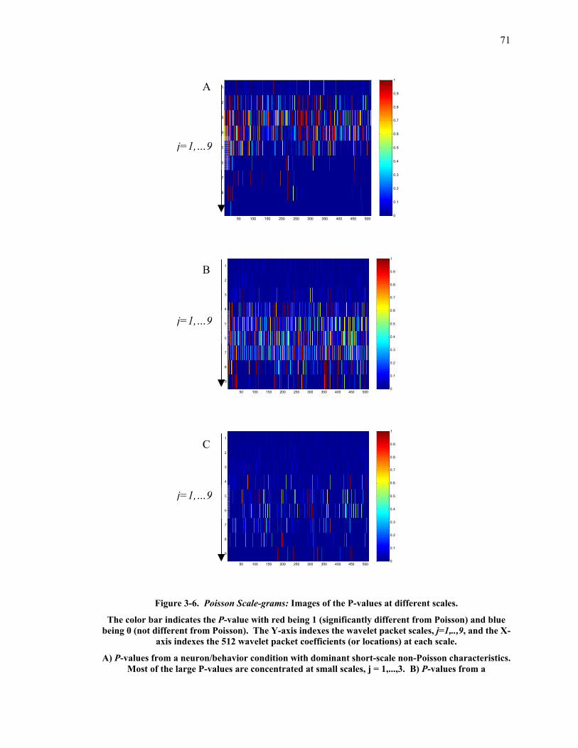
71
0
0.1
0.2
0.3
0.4
0.5
0.6
0.7
0.8
0.9
1
50 100 150 200 250 300 350 400 450 500
1
2
3
4
5
6
7
8
9
0
0.1
0.2
0.3
0.4
0.5
0.6
0.7
0.8
0.9
1
50 100 150 200 250 300 350 400 450 500
1
2
3
4
5
6
7
8
9
0
0.1
0.2
0.3
0.4
0.5
0.6
0.7
0.8
0.9
1
50 100 150 200 250 300 350 400 450 500
1
2
3
4
5
6
7
8
9
Figure 3-6. Poisson Scale-grams: Images of the P-values at different scales.
The color bar indicates the P-value with red being 1 (significantly different from Poisson) and blue being 0 (not different from Poisson). The Y-axis indexes the wavelet packet scales, j=1,..,9, and the X-
axis indexes the 512 wavelet packet coefficients (or locations) at each scale.
A) P-values from a neuron/behavior condition with dominant short-scale non-Poisson characteristics. Most of the large P-values are concentrated at small scales, j = 1,...,3. B) P-values from a
A
B
C
j=1,…9
j=1,…9
j=1,…9
72
neuron/behavior condition with dominant mid to large-scale non-Poisson characteristics. Most of the large P-values are concentrated at scales, j = 5,...,8. C) P-values from a neuron/behavior condition with relatively little non-Poisson characteristics. Most of the P-values at different scales are small.
It plots the Poisson scale-gram for one neuron/behavior combination that is representative
of the three types of behavior that we found in this set of PRR neurons. Evidently,
different neuron displays different characteristics on the Poisson Scale-gram. Some
resembles a Poisson process on a shorter time scale (10 ms); some have longer time
Poisson characteristics (200ms); others are Poisson over all time scales. This can be
completely captured by the Poisson Scale-gram as shown in Figure 3.7.
3.5 Conclusion
Understanding the statistical nature of a neuron’s spike generating processes is a crucial
step towards better understanding of the underlying neural code and constructing more
reliable neural controlled devices. In this chapter, a technique is proposed such that the
Haar wavelet packet projection is used to characterize the spike firing process because
the Haar wavelet packet carries some interesting properties that are particularly suitable
for strings of binary data. This approach, which is analogous to the Pyramid Algorithm,
computes the probabilities of wavelet packet projections given either homogeneous or
inhomogeneous Poisson process. Then it characterizes a spike train process by
comparing its wavelet packet coefficients’ probability distributions to the distributions of
a Poisson process with identical rate function. If the underlying process is indeed
Poisson, then the coefficients have distributions very close to its Poisson counterpart;
otherwise, significant deviation may be observed. Moreover, a Poisson scale-gram

73
(visualization method) is presented so that extra insight about the process’ scale of
Poisson-ness can be investigated. It allows us to infer the Poisson-ness of the process by
assessing at which scale it resembles a Poisson process. This chapter concludes with
several applications of the technique to both surrogate data and actual spike data from
PRR.
74
Chapter 4 Decoding Reach Direction Using Wavelet Packet
4.1 Introduction
In Chapter 1, we defined decoding as the task of inferring or estimating external stimuli
or behavioral states from neural signals [Abbot 1994, Rieke 1997]. Depending on the
specific problem at hand, the technical approaches to the decoding problem may vary
substantially. In one class of problems, a continuous stimulus parameter must be
decoded. In these cases, functional approximation techniques are exploited [Rieke 1997,
Brown 1998, Frank 2000]. At the other end of the spectrum lies the problem of decoding
discrete stimuli. For such problems, pattern recognition methods are employed
frequently [Georgopoulos 1986, Zhang 1997, Moran 1999, Schwartz 2000, Wessberg
2000, Issacs 2000, Nicolelis 2002]. Methods that accurately and efficiently decode
stimulus parameters given neural signals not only advance the state of bio-engineering
research, but also shed light on how the brain encodes information [Rieke 1997].
Pattern recognition, which is synonymous to classification, is the action of predicting or
classifying an unknown observation into predefined classes based on historical data. In
particular, decoding of a discretely valued stimulus using spike trains has been
investigated extensively in the context of pattern recognition. Researchers have applied
various pattern recognition techniques to treat the decoding problem. More importantly,
most of the current work uses the mean firing rate, the number of spike counts in a fixed
window, as the sole feature for decoding [Abbott 1994, Sanger 1996, Zhang 1998, Brown
1998, Johnson 1996, Reich 2000, Johnson 2001]. Here, feature refers to the patterns

75
embedded in the spike trains (e.g., mean firing rate, change of firing rate, and precise
timing of a particular spike) that are correlated to the stimulus parameter. However,
decoding based on firing rate alone assumes that no additional patterns exist in the spike
train, an oversimplified assumption [Steveninck 2002]. Thus, we ask whether any
improvements over either accuracy or resolution may be achieved when additional
features besides firing rate are included in the decoding task. The key issue thus becomes
that of finding the optimal feature(s) that ensure the best decoding performance.
To address this question, this chapter presents an adaptive scheme that searches for the
optimal feature(s) based on wavelet and information theory. Because different pattern
recognition methods behave differently even on the same set of data, in order to ensure
the comparability between the different features, we fix our classification tool to be the
Bayesian classifier introduced in Section 2.4. Under this scheme, a naïve feature set is
first generated using Haar wavelet packet decomposition of the spike trains. Because of
the recursive construction of wavelet packets, these features form a tree structure called
the wavelet packet coefficient tree. Then we suggest a tree pruning strategy that searches
for the most informative feature(s) along the coefficient tree with respect to the stimulus
parameters. Here, informative-ness is defined by a score function that quantifies the
feature’s discriminability towards the stimuli. The scored function proposed here is the
mutual information between the feature v and the stimuli label X because of its statistical
properties as well as its close relationship with the Bayesian classifier. The technique is
applied to both surrogate data and actual spike data. Decoding performance based on the

76
optimal feature(s) is compared against the performance obtained using mean firing rate
alone as the decoding feature.
Generally, wavelet-based analysis is more suitable when dealing with non-stationarity
and specifically locally stationary processes [Mallat, 1998]. As seen in Section 2.3, the
multi-resolution analysis feature of wavelets efficiently decomposes the spike trains into
features at different scales through projection, thus providing versatility in handling
possible patterns embedded in the spike train. Again, we use the Haar wavelet packet to
decompose the spike trains. Some of the Haar wavelet packet’s special properties, such
as compactness and biologically relevant interpretations of the projection coefficients,
make it an ideal candidate for decomposing spike trains. We note that others have
explored the possibility of using wavelet packet as a mean of processing spike data in the
decoding context [Kralik 2001]. But we are the first to investigate the decodability for
each individual wavelet packet coefficient.
When dealing with wavelet packet projection, often times the features, i.e. the projection
coefficients, are organized into a tree structure using the Pyramid Algorithm explained in
Section 2.3.2. Best Basis is an algorithm that prunes the coefficient tree in order to
search for an optimal set of bases for compression or denoising purpose [WickerHauser
1994, Mallat 1999, Percival and Walden 2001]. Saito (2002) presented a Best Basis
algorithm that searches for the most discriminating basis among the wavelet packet tree
using Kullback-Liebler distance as the discriminating measure. However, in the context
of decoding, the full optimal basis is less relevant as the curse of dimensionality results an
77
exponential explosion of the training data if the full basis is used for decoding. Thus, the
tree pruning method proposed in this chapter, although analogous to the Best Basis
algorithm, searches for a few features with large decodability instead of the full optimal
basis. Instead of finding the optimal sub-space upon which to project data, we are
looking for an optimal subset.
In Section 2, a study of the mutual information as the decodability score function is
presented. Then the wavelet packet tree based optimal feature extraction routine is
introduced. In Section 3, the technique developed earlier is applied to both surrogate data
and the actual spike data from PRR. This thesis assesses the performance of the proposed
method against that obtained by using mean firing rate alone. In the appendix, a
theoretical exposé on the finite sample effect is carried out for the two-class case in order
to further justify the use of mutual information as the score function. Even though all the
examples in this chapter use spike train data, the techniques proposed can be easily
generalized to other types of neural signals, such as the local field potential.
4.2 Feature extraction
As reviewed in Section 2.3, the wavelet packet decomposition returns a total of TlogT
features given a spike train that is quantized into T sampling periods of length δT. It is
however not realistic to include all the features in the decoding process because the curse
of dimensionality [Cherkasssky 1998] prohibits such a naïve approach. Moreover, very
few of these features are practically informative. Thus, we must select a few relevant
78
features in order to make practical decoding feasible. The selection strategy proposed
here involves a score function D, which assigns a discriminability measure to each
feature. Then we couple the score function with a pruning strategy that searches the Haar
wavelet packet coefficient tree while eliminating the less-informative coefficients. In the
following sections, we first investigate the use of mutual information as the score
function. Then we introduce the tree pruning strategy that searches for the most
informative features.
4.2.1 Discriminability and score functions
In order to assess the relevance of each projection coefficient, vjk, it is necessary to
introduce the concept of a score function D, which characterizes each feature’s
decodability. The score function is defined as a map from the feature’s conditional
probability distributions with respect to the stimulus parameter to a positive real number,
i.e.
Equation 4.1 +→×× RPPPD M...: 21 ,
where P1, P2,…,PM are short for the conditional probabilities P(v|X1), P(v|X2),…,
P(v|XM), with M being the number of stimulus classes available. Intuitively, the larger
the discrepancies between the Pi’s, the easier it is to classify different stimulus conditions
given an observation. Therefore, the score function should summarize the discrepancies
amongst all the conditional distributions with respect to the different stimulus parameters
Xi into a single discriminability number. For example, the Fisher linear discriminant
measure and the Kullbach-Liebler divergence are both frequently used discriminability
79
measures [Thomas and Cover 1991, Devroye 1996, Cherkassky 1998]. However, the
Fisher linear discriminant measure implicitly assumes the conditional distributions P1,
P2,…,PM are normally distributed, which constrains the statistical analysis to mean and
variance only. In addition, even though the KL divergence is a useful binary
classification measure, it lacks a multiple-class parallel. Researchers sometimes have to
resort to awkward pair-wise summations of the binary KL divergences between all
possible pairs of classes [Saito 2002]. Mutual information on the other hand does not
have the above undesirable features while possessing some nice interpretation and
properties. The remainder of the section introduces mutual information in the context of
decoding and assesses mutual information as the decodability measure. For interested
readers, an analysis of the finite sample effect and mutual information can also be found
in the appendix.
4.2.1.1 Mutual information overview
One choice of the score function is the mutual information between the features and the
classes, I(X;v). Mutual information characterizes the knowledge that one random
variable prescribes with respect to another [Thomas and Cover 1991]. To understand the
role of mutual information in the decoding context, it is necessary to define some relevant
information theoretical quantities.
For class variable X and feature v, define the Shannon entropy H(X) and the conditional
entropy H(X|v), two measures of information content as
80
Equation 4.2 ∑ ===
x ii XXP
XXPXH)(
1log)()( ,
Equation 4.3 ∑ =====
', )'|(1log)',()'|(
vi ii vvXXP
vvXXPvXH ,
where P(X=Xi) is the marginal probability of X, P(X=Xi|v=v’) is the conditional
probability of X when another random variable v takes the value v’, and P(X=Xi,v=v’) is
the joint probability between X and v [Cover and Thomas 1991]. We further notice the
following relationship between H(X) and H(X|v)
Equation 4.4
∑ ====
===
−=
', )'()()',(log)',(
)|()();(
vx vvPxXPvvxXPvvxXP
vxHxHvXI
,
where I(x,v) is the mutual information between the stimulus class X and the feature v.
Mutual information is also closely related to the Bayesian classifier as it can be directly
derived from the Bayes’ formula. Recall Equation 2.16 states that
)()()|()|(
vPXPXvPvXP = .
Manipulating this equation yields the following expression
)()()(
)()|()|( XPXPvP
XPXvPvXP = .
Taking the log of the above probability and the expected value over X and v on the above
equation yields the following,
Equation 4.5 )(log),()()(
),(log),()|(log),(,,,
XPvXPXPvP
XvPvXPvXPvXPvXvXvX
∑∑∑ += .
81
By the definition in Equation 4.2 and Equation 4.3, the above relationship is equivalent to
)();()|( XHvXIvxH −=− ,
the same relationship as Equation 4.4 again. Furthermore, recall from Equation 2.17, the
Bayesian classifier attempts to maximizes P(X|v) for every v. Thus, when taken over the
negative log expected value, it also minimizes the conditional entropy H(X|v), which in
turn maximizes the mutual information between X and v. Thus, we see Bayesian
classifier itself manifests an important information theoretical dogma: conditioning
reduces entropy.
The above analysis suggests that mutual information is an ideal candidate for the score
function D when the decoding tool is chosen to be the Bayesian classifier. In addition,
mutual information is closely related to the Bayesian classifier error E*, defined in
Equation 2.18. Assume there is no prior knowledge on the classes, i.e. the prior
probabilities on the classes are equal, then the mutual information between the classes
and features are bounded by the following relationship [Devroye 1998],
]1
1log)1(1log[1);()1log(1 **
***
EE
EEXvIE
−−+−≥≥−+ ,
where the right-hand side inequality is the Fano inequality and the left-hand side
inequality can be defined from Jensen’s inequality [Devroye 1998]. Evidently, large
mutual information corresponds to a smaller classification error. An in-depth
investigation on the classification error and the mutual information presented in the
Appendix further justifies the use of mutual information as the discriminability measure.
Mutual information also carries some additional useful statistical properties.
82
P1 Mutual information ),...,,;( 21 dvvvXI is invariant under an orthonormal
transformation, T , on the feature set V={v1,v2,…,vd}.
This can be easily verified as [Sirzaker 1994],
T T ⋅= )()( VPVP ,
where ( )dvvvV ,...,, 21= and T is the determinant of the T, which equals 1 when T is an
orthonormal matrix [Ross 2000]. Therefore, the value of the mutual information is
invariant under the transformation.
P2 Mutual information is additive, i.e.
∑=
=d
iid vXIvvvXI
121 );(),...,,;(
if the features v1, v2,…vd are conditionally independent (independent conditioned on the
stimulus parameter X) and unconditionally independent simultaneously (independent
without conditioning). We denote the conditionally and unconditionally independence as
CU-independence.
Finally, the definition of mutual information naturally accommodates multiple-class
classification problems without resorting to the awkward pair-wise sum often found in
other distance measures like KL-divergence or Hellinger distance [Saito 2002]. The
conditioning reduces entropy interpretation remains intact for multiple class applications.
83
4.2.1.2 Mutual information and optimal features
The above review on the mutual information I(X;v) not only justifies its use as a score
function for measuring discriminability, but also hints at the possibility of devising a
feature selection strategy. We notice that without any prior knowledge, the entropy
associated with the stimulus parameters X1, X2,…, XM is
)log()( MXH = ,
a fixed number independent of the features. Under this assumption, reducing the
conditional entropy H(X|v) is equivalent to increasing the mutual information I(X;v). As
H(X|v) approaches 0, X becomes almost deterministic given v. Therefore, the most
informative feature for the Bayesian classifier is the one that maximizes the mutual
information I(X;v). This important observation will be expanded and formalized in the
remainder of the section.
First we revisit the neural decoding problem. The task of decoding is to infer some
discrete behavior parameter X from an observed spike train s={s0,…sT-1}, given
historically collected spike train data under behavior states, X1,…,XM. The best possible
decoding strategy is to plug the whole observed spike train s into the Bayesian classifier
such that Equation 2.16 becomes
{ })|(maxarg~
sXPXX
= .
Here P(X|s) is the posterior probability which is proportional to the likelihood P(s|X). In
this case, no information is lost as the mutual information I(X;s) contains the full
knowledge that the spike train holds about the stimulus X. This is a version of the Data
84
Processing Inequality outlined in Thomas and Cover [1991]. However, in practice this
approach is not feasible because one needs to estimate the conditional probability P(s|X),
i.e. P(s0,…,sT-1|X). As T grows, the curse of dimensionality [Cherkassky 1998] demands
an exponential explosion of the training data in order to construct the joint distribution
P(s0,…,sT-1|X). Thus, it is not practically possible to use the full spike train s in the
Bayesian classifier.
An alternative alternative approach is to project the spike train onto some basis or feature
vectors such that the projection coefficients display large decodability. Then, instead of
the full spike train s, we include those selected features into the Bayesian classifier.
Formally, we denote an orthonormal transformation as T such that
Equation 4.6 sv ⋅= T ,
where v={v0,…,vT-1} is the projection coefficients of s onto the basis vectors of T. By
property P1, mutual information is invariant under this transformation,
Equation 4.7 ),();( vs XIXI = .
In addition, if the components of v, v0,…,vT-1 are CU independent, then by property P2,
Equation 4.8 ∑−
=− =
1
011 );(),...,,;(
T
iiTo vXIvvvXI .
Thus, ideally, the suggested feature extraction method will focus on finding a
transformation, T *, such that the following criterion is satisfied: the d CU independent
projection coefficients *1
*0 ,..., −dvv preserve most of the mutual information, namely
∑−
=
≈1
0
* );();(d
ii XIvXI s .
85
Because of the independence as well as the reduction of dimensionality, estimating the
corresponding conditional probabilities )|( * XvP i will not result in the explosion of the
number of training samples required as seen in the curse of dimensionality. In Section
4.2.2, we explore some techniques that extract the features v0,…,vd-1 under the Haar
wavelet packet transformation framework.
4.2.1.3 Estimating the mutual information
To compute mutual information, the conditional probability p(v|X) must be estimated. As
shown in Section 2.4, Parzen window method is used [Parzen 1965]. The Parzen window
approach applies Gaussian kernels to the observed data and returns density estimation in
the form of the normalized sum of Gaussians centered at each data point. One can write
the density function estimated by his approach as
∑=
−==cN
ii
c
vvGN
cXvp1
),(1)|( σ
where G(v, σ) is a Gaussian kernel with mean vi ( the observed data in class X=c) and
standard deviation σ, and Nc is the total number of trials in class Xc. Clearly p(v|X=c) is a
density function because it integrates to 1 over all values of v. Therefore, we can use the
Parzen window approximation in place of the true conditional density functions (which is
unavailable) to estimate the mutual information. The choice of σ controls the smoothness
of the probability density. We observe that when σ is sufficiently small, the mutual
information is equivalent to the one computed using the histogram rule, namely,
∑=
===cN
ii
ci vIn
NcXvvP
1)(1)|( ,
86
where In(vi) is the indicator function,
=
=otherwise
vvifvIn i
i 01
)( .
Generally, we keep the value of σ small when the scales of the wavelet coefficients are
small and vice versa.
4.2.2 Wavelet packet tree pruning
The previous section defined mutual information as the score function, D, that assesses
the discriminability of features, v, with respect to the stimulus parameter X. Moreover,
the theoretical analysis of the mutual information I(X;v) suggests a feature extraction
approach that searches for an orthonormal transformation T on the spike train s such that
a few independent transformed features *1
*0 ,..., −dvv preserve most of the mutual
information I(X;s). This section realizes this proposition by introducing a feature
selection strategy that integrates mutual information with the Haar wavelet packet. The
selection strategy adopted here is analogous to the Best Basis algorithm used in the signal
processing and data compression community [Wickerhauser 1994, Mallat 1999, Percival
and Walden 2001]. Moreover, Saito and Coifman suggested a most discriminating Best
Basis method in a different context [Saito 2002]. However, unlike the Best Basis
algorithm, our approach searches for the d most discriminating features instead of a full
basis.
As seen in Section 2.3.3, the cardinality of the Haar wavelet packet coefficients given a
spike train of length T is TlogT. In addition, the construction of the Haar wavelet packet
87
ensures that the member functions within a node and between different nodes are
orthogonal (Proposition 2.1). This poses a challenge when the optimal basis for some
signal processing criterion (de-noising, compression, etc.) is required because searching
through all the possible collections of orthonormal functions causes a combinatorial
explosion. The Best Basis algorithm is an efficient technique that prunes the wavelet
packet tree and evaluates the applicability of each node in the tree by comparing it with
its parent node, using an additive score function [Wickhauser 1994]. In the case of the
most discriminating Best Basis algorithm [Saito 2002], the score function is chosen as the
pair-wise summation of Kullbach-Liebler divergences between all the conditional
probabilities P(v|Xi) and P(v|Xj).
Our approach on the other hand looks for the d most discriminating features instead of
the full basis. Recall from Section 4.2.1.2 that we ideally seek a transformation T * such
that the d largest CU-independent projection coefficients *1
*0 ,..., −dvv preserve most of the
mutual information, namely,
∑−
=
≈1
0
* );();(d
ii XIvXI s .
However, because I(X;s) is difficult to compute in practice and CU independence is a
stringent requirement, it is necessary to either use the sufficient condition for the
constraints or modestly relax the above constraints for practical implementation. First,
note that orthogonality is a necessary condition for the independence between the
features. To see this, define two non-orthogonal random variables v1 and v2. Because
they are not orthogonal, v1 can be expressed as the weighted sum of v2 and a residual term
vres , i.e.
88
resbvavv += 21 .
Obviously, v1 and v2 are dependent and the level of dependence is determined by the
weight a. Thus non-orthogonality implies non-independence, and the first modification
of the constraint is that the wavelet packet functions associated with the selected features
have to be mutually orthogonal. Another observation is that the mutual information of
the member coefficients of the parent node Njl equal that of the two children nodes N(j+1)2l
and N(j+1)(2l+1),
{ } { } { }])|,|[;(])|[;( )12)(1(2)1(11 +++++ ∈∈=∈ ljjkjkljkjkjjljkjk NvvNvvXINvvXI .
The validity of this equation relies on the fact that the coefficients
{ } { }]|,|[ )12)(1(112)1(11 +++++++ ∈∈ ljkjkjljkjkj NvvNvv can be obtained via an orthogonal
transformation on the coefficients { }]|[ jljkjk Nvv ∈ as seen in the nature of the Pyramid
Algorithm (Section 2.3) and property P1. In another words, the coefficients in the two
children nodes are orthonormal transformations of the ones in the parent node; thus the
associated mutual informations are invariant. Ideally, we would like to find a few
features from either the parent node Njl or the two children nodes N(j+1)2l and N(j+1)(2l+1) so
that the sum of their mutual information is close to the overall mutual information,
{ }])|[;( jljkjk NvvXI ∈ . However, the node mutual information { }])|[;( jljkjk NvvXI ∈ is
difficult to calculate and the CU-independence is hard to satisfy in general. Thus our
second relaxed constraint is that instead of keeping a few CU-independent features,
*1
*0 ,..., −mvv i.e.
89
{ }∑−
=
∈≈1
0
* )|;();(m
ijljkjki NvvXIvXI
where
{ })12)(1(,2)1(*
1*0 ,..., +++− ∈ ljljjld NNorNvv ,
only the one with the largest discriminability score among the parent and children nodes
should be retained, namely
{ }),|max( )12)(1(,2)1(*
+++∈= ljljjljkjk NNNvvv .
In summary, the two relaxed constraints are
Constraint 1: The wavelet packet functions that correspond to the optimal features have to
be orthogonal to each other.
Constraint 2: The single most informative feature in any pairs of parent-children nodes
must be included.
Now we are ready to describe out recursive wavelet packet pruning technique. Let the
training spike train ensembles be denoted by { } { } { }iM
ii SSS ,...,, 21 , where the subscript
corresponds to the stimulus parameters X1,…,XM. Furthermore, assume the spike trains in
the ensembles are of length T, where T is a power of 2. Using the Pyramid Algorithm,
the Haar wavelet packet projection coefficients at any scale j and location k can be
computed. These coefficients are called the naïve feature set, and they are naturally
organized in the tree structure seen in Section 2.3.2. Denote the tree associated with the
decomposition as the feature tree, F. Now starting from the coarsest scale, i.e.

90
Tj 2log= , first compute the score function D for the feature set { }jkv with j=log2T
whose score function for { }jkv is defined as
Equation 4.9 ∑∑ ∑=
v XX
jk
jkjkjk XpXvp
XvpXpXvpD
)()|()|(
log)()|(
and form a discriminability set { }jkD for each k. The conditional probability p(vjk|X) is
estimated using the Parzen window method shown in Section 4.2.1.3. Also we seed the
optimal feature set as
Equation 4.10 { } { }jkoptk vv = ,
i.e. to start, the optimal feature set is initialized to be the jth scale projection coefficients
because they are the descendants of the rest of the coefficients. Next we proceed to the j-
1th scale, where we again compute the score functions D for each feature vj-1,k and form
the discriminability set { }kjD ,1− . For each triplet of parent-children nodes
{ })12(,,2,),1( , +− ljljlj NNN , l=0,..T/2-1, we can find the feature v* with the largest
discriminating measure,
{ }),|max( )12(),1(,2),1(,*
+++∈= ljljljjkjk NNNvvv .
Once it is located, the node that contains v* is labeled N* and we can replace the
corresponding features in the set { }optkv by the ones in N*. For example, if ljNN ),1(
*−= ,
then
{ }{ } { }*),1(),1()12(,2, |,| NvvNNvv kjkjljlj
optk
optk ∈=∈ −−+ ,
effectively the optimal feature set { }optkv is updated to include all the features in N* along
with v*. As a result, we remove the node Nj,2l and Nj,(2l+1) from the original feature tree,
91
F. On the other hand, if )12(,2,*
+= ljlj NorNN , then no update of { }optkv occurs and
both Nj,2l and Nj,(2l+1) remains on the feature tree, F. Once the update is completed at
scale j-1, we move up to scale j-2 and repeat the above process by comparing the parent
node Nj-2,l with its remaining descendents. Again, the optimal feature set { }optkv as well
the tree F is updated. This procedure terminates when the updates on { }optkv terminates
and F is no longer modified. Also the Haar wavelet packet functions associated with the
features { }optkv are orthogonal to each other because of Proposition 2.1. Graphically, we
may express the pruning procedure in Figure 4.1:
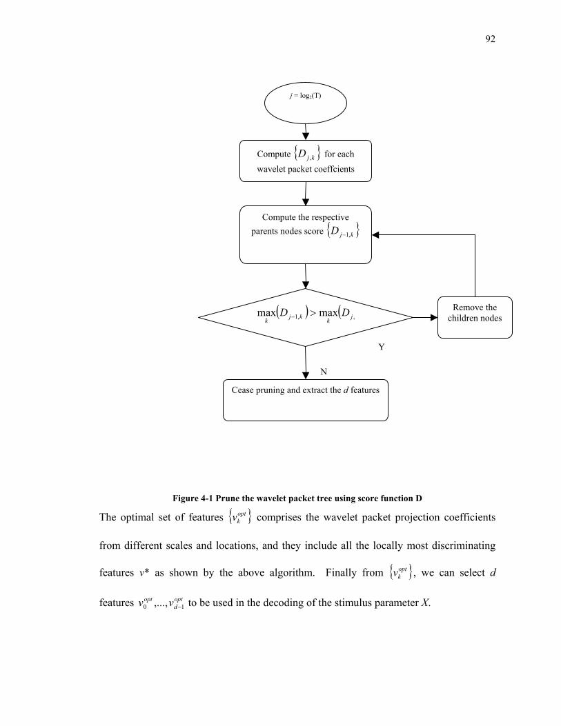
92
Figure 4-1 Prune the wavelet packet tree using score function D
The optimal set of features { }optkv comprises the wavelet packet projection coefficients
from different scales and locations, and they include all the locally most discriminating
features v* as shown by the above algorithm. Finally from { }optkv , we can select d
features optd
opt vv 10 ,..., − to be used in the decoding of the stimulus parameter X.
j = log2(T)
Compute { }kjD , for each wavelet packet coeffcients
Compute the respective parents nodes score { }kjD ,1−
Remove the children nodes
Y
N
( ) ( kjkkjkDD ,,1 maxmax >−
Cease pruning and extract the d features
93
In practice, the d features not only need to carry large discriminating scores, but also
should be evaluated for conditional independence because as we pointed out earlier,
orthogonality is only a necessary condition for independence. We can use hypothesis test
methods (e.g., cross-tabulation by Mathworks) to help understand the dependence
between features so that a minimal amount of redundant information is included in the
decoding process. At the current stage, properties of optd
opt vv 10 ,..., − will be assessed on an
individual basis for each application. In addition, a good way of picking the number d is
currently lacking. Rather, it varies depending on the actual application. However, as we
will see in the results section, even by letting d=1, the single most informative feature
often outperforms the mean firing rate.
4.3 Results
This section applies the above ideas and algorithms to both surrogate data sets and actual
behavior conditioned spike trains in order to illustrate the utility of the method. First
examine the application of the algorithm to artificial data with different discriminating
features. These simulations confirm the basic operation of the approach. Next apply the
method to actual neural data recorded in PRR. In both cases, we compare the decoding
performance of our method against the performance obtained using mean firing rate as
the only feature.
Inhomogeneous Poisson Processes I
We first investigate the performance of the proposed decoding method on surrogate data
generated from known inhomogeneous Poisson processes. The surrogate data are
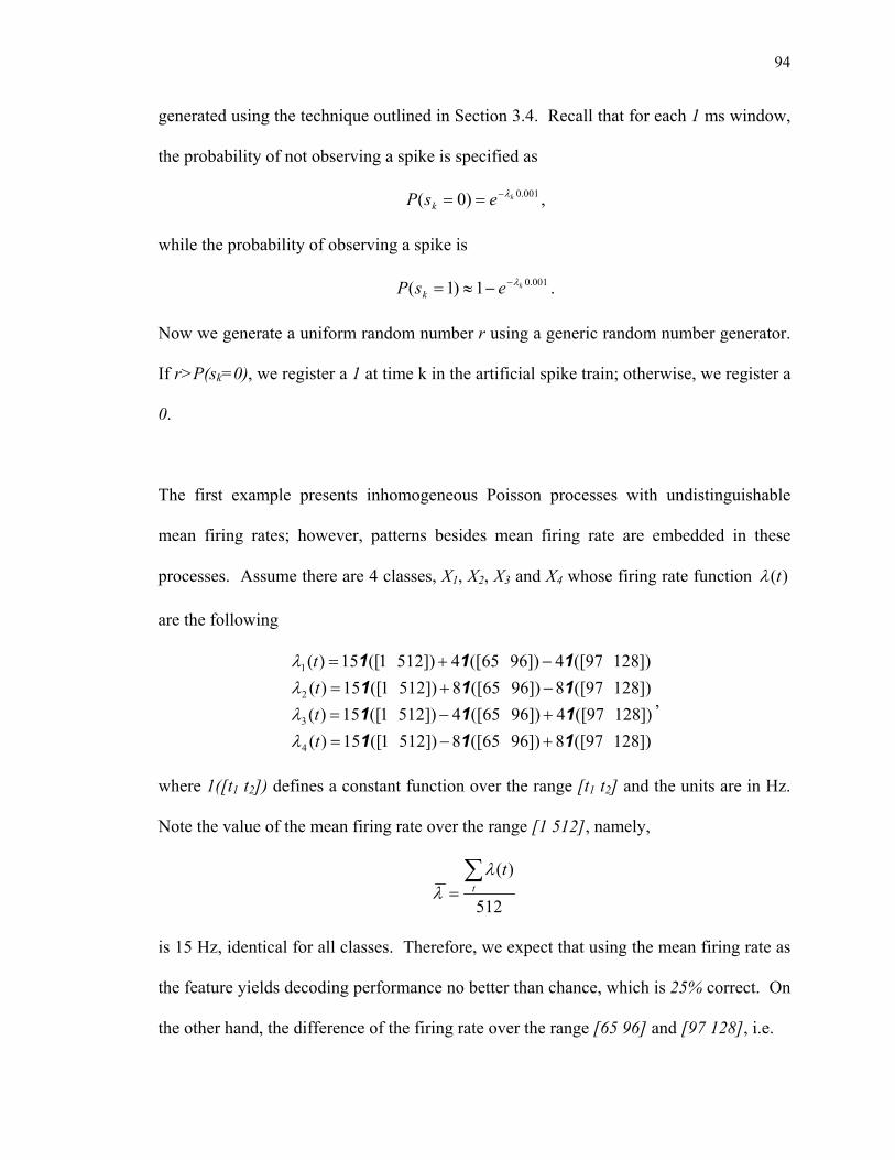
94
generated using the technique outlined in Section 3.4. Recall that for each 1 ms window,
the probability of not observing a spike is specified as
001.0)0( kesP kλ−== ,
while the probability of observing a spike is
001.01)1( kesP kλ−−≈= .
Now we generate a uniform random number r using a generic random number generator.
If r>P(sk=0), we register a 1 at time k in the artificial spike train; otherwise, we register a
0.
The first example presents inhomogeneous Poisson processes with undistinguishable
mean firing rates; however, patterns besides mean firing rate are embedded in these
processes. Assume there are 4 classes, X1, X2, X3 and X4 whose firing rate function )(tλ
are the following
])12897([8])9665([8])5121([15)(])12897([4])9665([4])5121([15)(])12897([8])9665([8])5121([15)(])12897([4])9665([4])5121([15)(
4
3
2
1
111111111111
+−=+−=−+=−+=
tttt
λλλλ
,
where 1([t1 t2]) defines a constant function over the range [t1 t2] and the units are in Hz.
Note the value of the mean firing rate over the range [1 512], namely,
512
)(∑= t
tλλ
is 15 Hz, identical for all classes. Therefore, we expect that using the mean firing rate as
the feature yields decoding performance no better than chance, which is 25% correct. On
the other hand, the difference of the firing rate over the range [65 96] and [97 128], i.e.

95
32
)()(128
97
96
65∑∑==
−= tt
ttf
λλ,
yields the most discriminating feature because the firing rate at each time step is the only
modulated parameter for an inhomogeneous Poisson process [Ross 1994]. The sum of
the difference of the firing rates thus becomes the best discriminating feature.
The wavelet packet decoding method is applied to spike trains generated according to the
above firing rate functions. For each class, the aforementioned simulation algorithm
produces 500 training samples and 500 testing samples. The following test and analysis
is done on the 500 testing samples and the average performance is reported. The optimal
selection strategy outlined in Section 4.2.2 returns 512 features that are the projections of
the spike trains onto the selected orthonormal Haar wavelet packet basis functions. The
values of the mutual information associated with these features are plotted in Figure
4-2A. The wavelet packet function corresponds to the largest mutual information (red
circle in Figure 4-2A) is plotted in Figure 4-2B. It indeed agrees with the aforementioned
feature f. In addition, the distribution of mean firing rate and the optimal feature are
shown in Figure 4-2C.
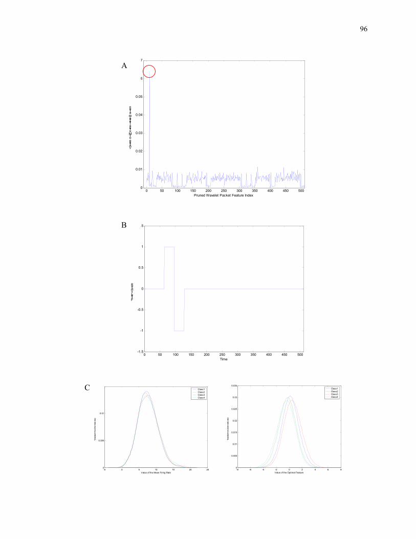
96
0 50 100 150 200 250 300 350 400 450 5000
0.01
0.02
0.03
0.04
0.05
0.06
0.07
Value of Mutual Information
Pruned Wavelet Packet Feature Index
0 50 100 150 200 250 300 350 400 450 500-1.5
-1
-0.5
0
0.5
1
1.5
Time
Filter Value
-5 0 5 10 15 20 250
0.005
0.01
0.015
Value of the Mean Firing Rate
Probability Distribution
Class1Class2Class3Class4
-8 -6 -4 -2 0 2 4 6 80
0.005
0.01
0.015
0.02
0.025
0.03
0.035
Value of the Optimal Feature
Probability Distribution
Class1Class2Class3Class4
B
A
C
97
Figure 4-2 Application of the optimal wavelet packet to the surrogate data
A) The value of mutual information of the pruned wavelet packet features. The x-axis indexes the 512 wavelet packet functions, while the Y-axis indicates the value of the corresponding mutual
information. B) The wavelet packet function with the largest mutual information. X-axis is time, and Y-axis is its value. C) The distribution of the mean firing rate and the optimal wavelet packet feature. The panel on the left displays the mean firing rate distribution of the training data; the
panel on the right shows the optimal feature. In both figures, the x-axis is the value of the coefficients and the y-axis is its distribution. Color codes the 4 classes.
To validate the optimal feature, we apply the Bayesian classifier to the training data using
both the optimal feature vopt as well as the mean firing rate λ . Not surprisingly, the one
using mean firing rate returns an average correct classification of 25%, exactly on par
with chance. On the hand, the optimal feature on average returns correct classification of
33%. While this result may not seem impressive, it should be recognized that these
classes are extremely similar, and therefore difficult to discriminate.
Inhomogeneous Poisson Processes II
We can also augment the above firing rate function to include a discriminating feature
that describes precise timing in a spike train. For each previously generated surrogate
spike train, we embed a single spike at a specific location in a background of spikes
generated from a Poisson process. We use the following equations to illustrate this
important addition to our surrogate data,
1)(),(~)( =τλ sandtts ,
where s(t) is the spike train generated from the firing rate function λ(t), and τ marks the
location of the single precise spike. We continue the previous example and let the τ’s be
τ1=1, τ2=5, τ3=9, and τ4=13, the subscripts index the four classes. Once again, the
surrogate data contain 500 training and testing spike trains for each reach direction. We
apply the method illustrated in Section 4.2.2 to the surrogated data and obtain the optimal
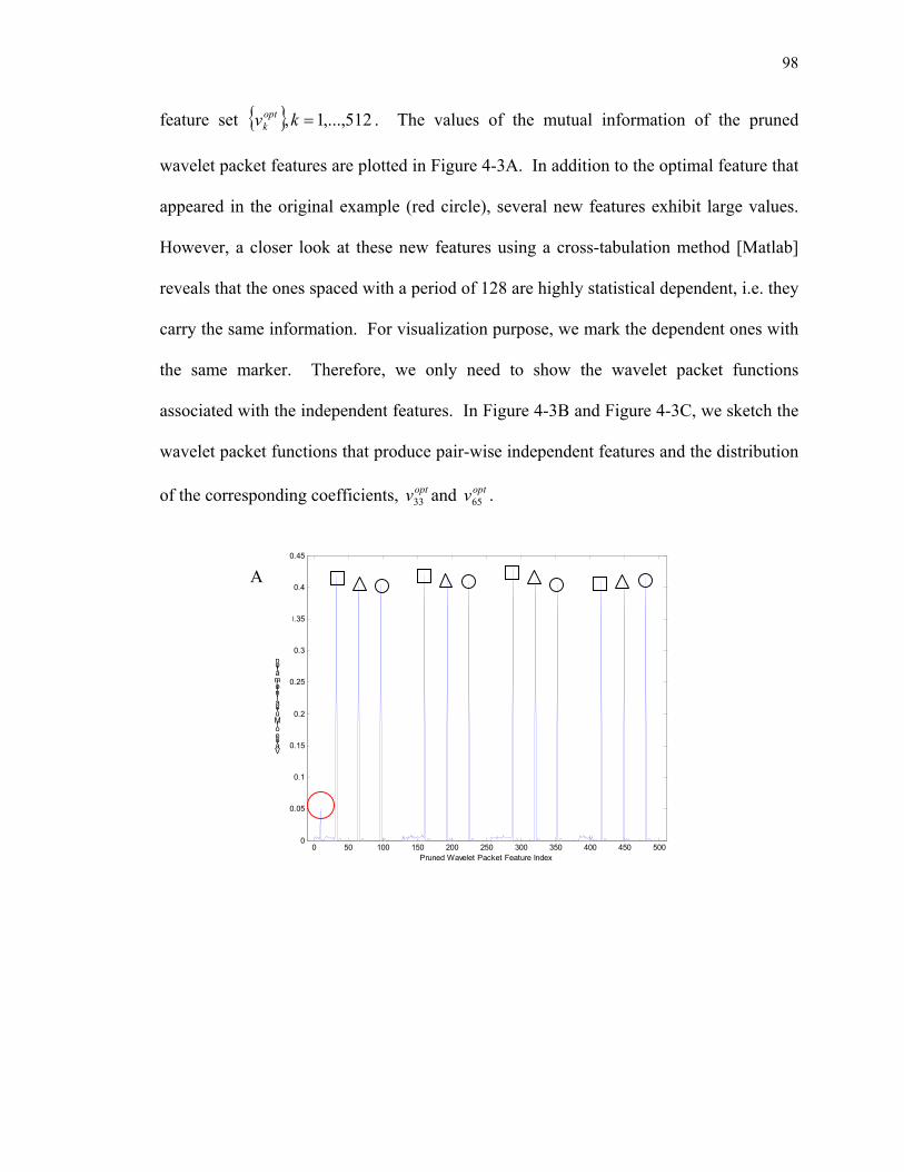
98
feature set { } 512,...,1, =kvoptk . The values of the mutual information of the pruned
wavelet packet features are plotted in Figure 4-3A. In addition to the optimal feature that
appeared in the original example (red circle), several new features exhibit large values.
However, a closer look at these new features using a cross-tabulation method [Matlab]
reveals that the ones spaced with a period of 128 are highly statistical dependent, i.e. they
carry the same information. For visualization purpose, we mark the dependent ones with
the same marker. Therefore, we only need to show the wavelet packet functions
associated with the independent features. In Figure 4-3B and Figure 4-3C, we sketch the
wavelet packet functions that produce pair-wise independent features and the distribution
of the corresponding coefficients, optv33 and optv65 .
0 50 100 150 200 250 300 350 400 450 5000
0.05
0.1
0.15
0.2
0.25
0.3
0.35
0.4
0.45
Pruned Wavelet Packet Feature Index
Value of Mutual Information
A
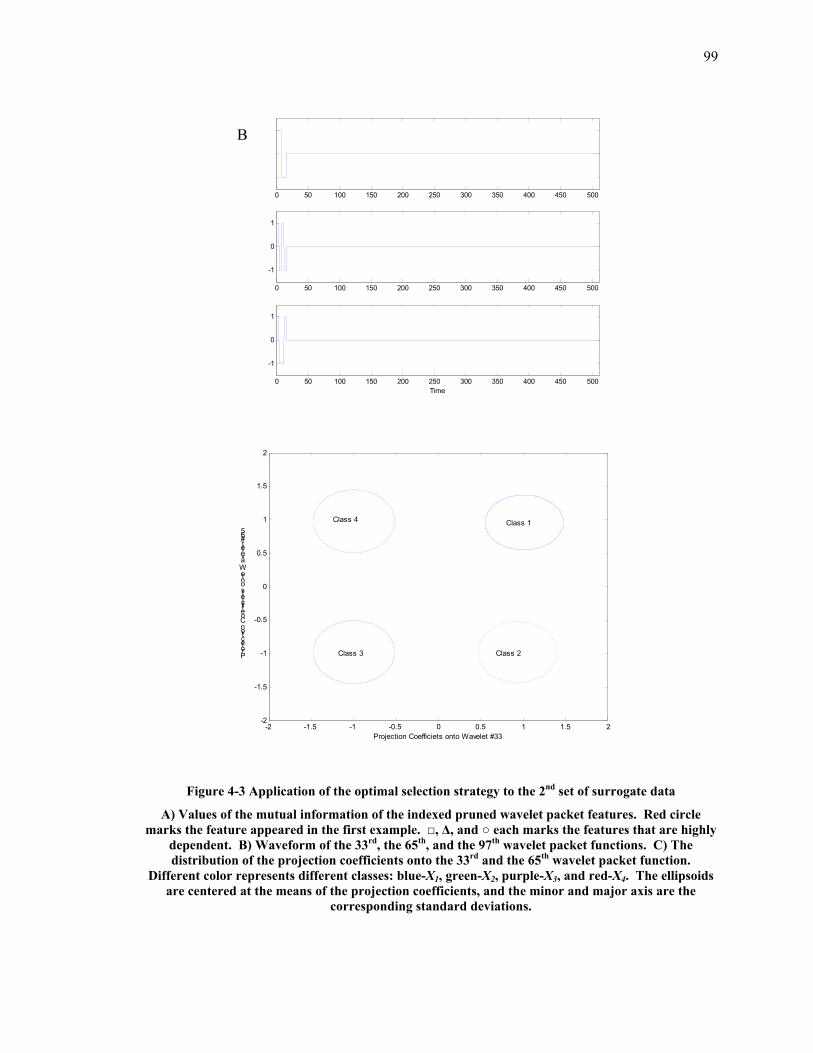
99
0 50 100 150 200 250 300 350 400 450 500
-1
0
1
0 50 100 150 200 250 300 350 400 450 500
-1
0
1
0 50 100 150 200 250 300 350 400 450 500
-1
0
1
Time
-2 -1.5 -1 -0.5 0 0.5 1 1.5 2-2
-1.5
-1
-0.5
0
0.5
1
1.5
2
Projection Coefficiets onto Wavelet #33
Projection Coefficiets onto Wavelet #65
Class 1
Class 2 Class 3
Class 4
Figure 4-3 Application of the optimal selection strategy to the 2nd set of surrogate data
A) Values of the mutual information of the indexed pruned wavelet packet features. Red circle marks the feature appeared in the first example. □, ∆, and ○ each marks the features that are highly
dependent. B) Waveform of the 33rd, the 65th, and the 97th wavelet packet functions. C) The distribution of the projection coefficients onto the 33rd and the 65th wavelet packet function.
Different color represents different classes: blue-X1, green-X2, purple-X3, and red-X4. The ellipsoids are centered at the means of the projection coefficients, and the minor and major axis are the
corresponding standard deviations.
B
100
Note that the wavelet packet functions not only cover the region of interest [1,16], but
also separate the 4 different classes. Observe that the separation of the classes on the two
dimensional probability plane shown in Figure 4-3C allows for good classification
outcome. On the contrary, using mean firing rate over the whole 512ms window in this
example completely ignores the information coded in the precise spike location. Thus,
just as the previous example, the decoding performance using the mean firing rate fares
no better than chance while the feature extraction method displays better decoding
performance. In this example, the decoding performance rises from chance (25%) to
91%, as exemplified by the separation of features among the 4 classes in Figure 4.3C.
PRR Spike Trains during Reach Task I
Next the method is applied to decode actual spike signals recorded from PRR during
reach tasks. The experimental paradigm is described in Section 2.1. Here we focus on a
particular 512ms window which is 300ms after the cue onset. The data is sampled at a
sampling interval of 1ms. The biological importance for this particular time window is
that reach intention is formed during that period [Batista 1999, Shenoy 2003]. There are
a total of 15 neurons, each with 2 reach conditions, X1 and X2. The number of samples
ranges from 25 to 115. Because of the limited samples, the classification of the reach
condition given an unknown spike train uses the leave-one-out cross-validation method
[Cherkassky 1998]. It singles out one sample as the test sample and use the remaining
ones as the training sample to classify the test sample.

101
And example of the spike trains from one neuron along with the most informative
wavelet packet feature is shown in Figure 4.4A.
0 50 100 150 200 250 300 350 400 450 5000
5
10
15
20
25
Time ms
Trials of Spike Trains
0 50 100 150 200 250 300 350 400 450 5000
5
10
15
20
25
30
35
40
Time ms
Trials of Spike Trains
0 50 100 150 200 250 300 350 400 450 5000
0.5
1
1.5
Time
Value
-5 0 5 10 15 20 250
0.002
0.004
0.006
0.008
0.01
0.012
0.014
Mean Firing Rate Value
Probability
-4 -2 0 2 4 6 8 100
0.005
0.01
0.015
0.02
0.025
0.03
0.035
Projection Coefficient Value
Probability
Figure 4-4 Comparison of mean firing rate and optimal wavelet packet feature for a neuron in binary reach task
A) The two panels showcase the neuron’s spike trains in two different reach conditions. The x-axis marks the time in millisecond and the y-axis indexes the trial number. B) The optimal wavelet
B
A
C
102
packet function with a support of 128ms, ( j = 7, k=1). The x-axis marks the time in milliseconds, and the y-axis is the value of the function. C) The left panel shows the distribution of the mean firing
rate given the two different reach directions. Each color represents a reach direction. X-axis is the value of the coefficients and y-axis marks the probabilities. The right panel displays the optimal
feature distribution for the same two reach directions.
In the above example, we can visually identify from Figure 4-4A that the neurons fire
more frequently in the first 100ms in one direction than the other one. The optimal
wavelet packet feature selected in this case is a window function corresponding to the
first 128ms. Evidently, the discriminability of the optimal feature surpasses the ones of
the mean firing rate because the two conditional distribution functions are further apart,
as demonstrated in Figure 4-4C. Fittingly the correct classification rate using the mean
firing rate is 36.7%, while the optimal feature approach realizes a 72% correct rate. Note
the reason for the sub-50% decoding performance of the mean firing rate case can be
contributed to the cross-validation technique. For each cross-validation, the training
distribution is rebuilt by taking out the test sample from the whole ensemble. For sparse
data sets, this results a large reduction of the prior probability P(v|X); thus numerically, it
is possible to achieve sub-50% performance.
Within the wavelet packet feature selection framework, we can also assess the effect of
mutual information by replacing the score function with the Fisher linear discriminant
measure [Fisher 1936], DFisher, which is defined as
( )22
2
221
1σσ +
−=
mmDFisher ,
where m1 and m2 are the means of the data points belonging to class 1 and class2; σ1 and
σ2 are the respective standard deviations. Obviously DFisher is large when the two clusters
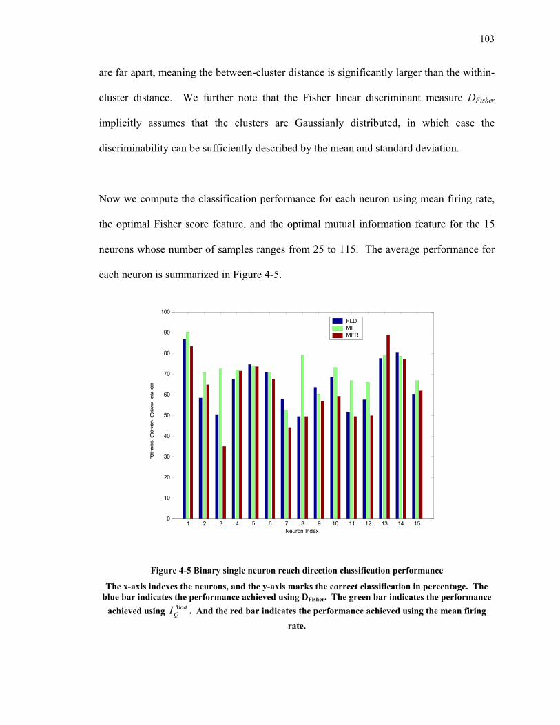
103
are far apart, meaning the between-cluster distance is significantly larger than the within-
cluster distance. We further note that the Fisher linear discriminant measure DFisher
implicitly assumes that the clusters are Gaussianly distributed, in which case the
discriminability can be sufficiently described by the mean and standard deviation.
Now we compute the classification performance for each neuron using mean firing rate,
the optimal Fisher score feature, and the optimal mutual information feature for the 15
neurons whose number of samples ranges from 25 to 115. The average performance for
each neuron is summarized in Figure 4-5.
1 2 3 4 5 6 7 8 9 10 11 12 13 14 150
10
20
30
40
50
60
70
80
90
100
Neuron Index
Percent Correct Classification
FLDMIMFR
Figure 4-5 Binary single neuron reach direction classification performance
The x-axis indexes the neurons, and the y-axis marks the correct classification in percentage. The blue bar indicates the performance achieved using DFisher. The green bar indicates the performance
achieved using ModQI . And the red bar indicates the performance achieved using the mean firing
rate.
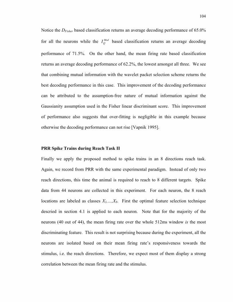
104
Notice the DFisher based classification returns an average decoding performance of 65.0%
for all the neurons while the ModQI based classification returns an average decoding
performance of 71.5%. On the other hand, the mean firing rate based classification
returns an average decoding performance of 62.2%, the lowest amongst all three. We see
that combining mutual information with the wavelet packet selection scheme returns the
best decoding performance in this case. This improvement of the decoding performance
can be attributed to the assumption-free nature of mutual information against the
Gaussianity assumption used in the Fisher linear discriminant score. This improvement
of performance also suggests that over-fitting is negligible in this example because
otherwise the decoding performance can not rise [Vapnik 1995].
PRR Spike Trains during Reach Task II
Finally we apply the proposed method to spike trains in an 8 directions reach task.
Again, we record from PRR with the same experimental paradigm. Instead of only two
reach directions, this time the animal is required to reach to 8 different targets. Spike
data from 44 neurons are collected in this experiment. For each neuron, the 8 reach
locations are labeled as classes X1,…,X8. First the optimal feature selection technique
descried in section 4.1 is applied to each neuron. Note that for the majority of the
neurons (40 out of 44), the mean firing rate over the whole 512ms window is the most
discriminating feature. This result is not surprising because during the experiment, all the
neurons are isolated based on their mean firing rate’s responsiveness towards the
stimulus, i.e. the reach directions. Therefore, we expect most of them display a strong
correlation between the mean firing rate and the stimulus.
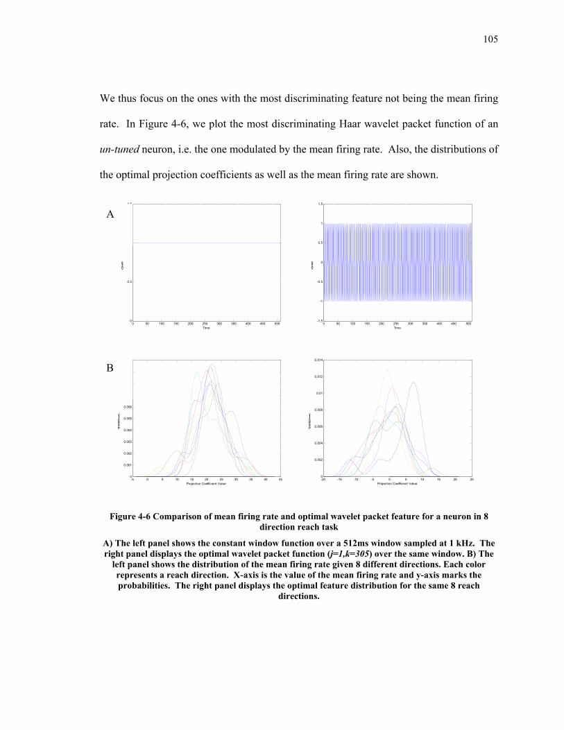
105
We thus focus on the ones with the most discriminating feature not being the mean firing
rate. In Figure 4-6, we plot the most discriminating Haar wavelet packet function of an
un-tuned neuron, i.e. the one modulated by the mean firing rate. Also, the distributions of
the optimal projection coefficients as well as the mean firing rate are shown.
0 50 100 150 200 250 300 350 400 450 5000
0.5
1
1.5
Time
Value
0 50 100 150 200 250 300 350 400 450 500-1.5
-1
-0.5
0
0.5
1
1.5
Time
Value
-5 0 5 10 15 20 25 30 35 40 450
0.001
0.002
0.003
0.004
0.005
0.006
0.007
0.008
0.009
0.01
Projection Coefficient Value
Probability
-20 -15 -10 -5 0 5 10 15 20 250
0.002
0.004
0.006
0.008
0.01
0.012
0.014
Projection Coefficient Value
Probability
Figure 4-6 Comparison of mean firing rate and optimal wavelet packet feature for a neuron in 8 direction reach task
A) The left panel shows the constant window function over a 512ms window sampled at 1 kHz. The right panel displays the optimal wavelet packet function (j=1,k=305) over the same window. B) The
left panel shows the distribution of the mean firing rate given 8 different directions. Each color represents a reach direction. X-axis is the value of the mean firing rate and y-axis marks the probabilities. The right panel displays the optimal feature distribution for the same 8 reach
directions.
A
B
106
Note in Figure 4-6B that the conditional distributions of the optimal coefficients are more
spread out than their mean firing rate counterpart. This validates the argument in Section
4.2.2 that the feature chosen using mutual information corresponds to better
discriminability.
Moreover, the average single neuron Bayesian decoding performance of 4 un-tuned
neurons and the combined decoding performance of the 4 neurons are shown in Figure
4-7 using the leave-one-out cross-validation method [Cherkassky 1998]. The 4 un-tuned
neurons are combined for decoding using the Bayesian classifier,
∏ ==)(
)()|()|( 4
1ineruon
ineuroni vP
XPXvPVXP ,
where X is the class label, V={vneruon 1,…vneuron 4} is the feature vector for all 4 neurons,
P(X|V) is the posterior probability, P(X) is the prior probability of X, and P(V|X) is the
likelihood of V given X, and
{ })|(maxarg~
VXPXX
= .
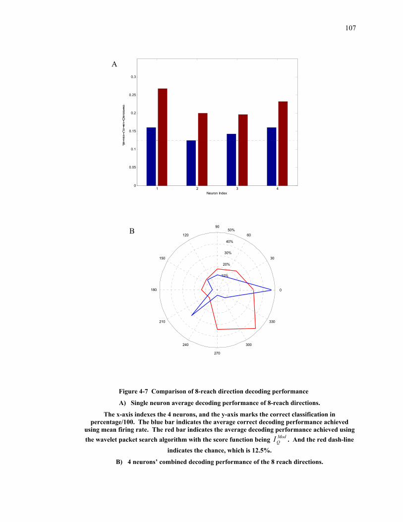
107
1 2 3 40
0.05
0.1
0.15
0.2
0.25
0.3
Neuron Index
Percent Correct Decoding
10%
20%
30%
40%
50%
30
210
60
240
90
270
120
300
150
330
180 0
Figure 4-7 Comparison of 8-reach direction decoding performance
A) Single neuron average decoding performance of 8-reach directions.
The x-axis indexes the 4 neurons, and the y-axis marks the correct classification in percentage/100. The blue bar indicates the average correct decoding performance achieved
using mean firing rate. The red bar indicates the average decoding performance achieved using the wavelet packet search algorithm with the score function being Mod
QI . And the red dash-line indicates the chance, which is 12.5%.
B) 4 neurons’ combined decoding performance of the 8 reach directions.
A
B
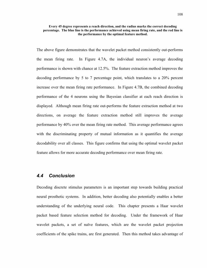
108
Every 45 degree represents a reach direction, and the radius marks the correct decoding percentage. The blue line is the performance achieved using mean firing rate, and the red line is
the performance by the optimal feature method.
The above figure demonstrates that the wavelet packet method consistently out-performs
the mean firing rate. In Figure 4.7A, the individual neuron’s average decoding
performance is shown with chance at 12.5%. The feature extraction method improves the
decoding performance by 5 to 7 percentage point, which translates to a 20% percent
increase over the mean firing rate performance. In Figure 4.7B, the combined decoding
performance of the 4 neurons using the Bayesian classifier at each reach direction is
displayed. Although mean firing rate out-performs the feature extraction method at two
directions, on average the feature extraction method still improves the average
performance by 40% over the mean firing rate method. This average performance agrees
with the discriminating property of mutual information as it quantifies the average
decodability over all classes. This figure confirms that using the optimal wavelet packet
feature allows for more accurate decoding performance over mean firing rate.
4.4 Conclusion
Decoding discrete stimulus parameters is an important step towards building practical
neural prosthetic systems. In addition, better decoding also potentially enables a better
understanding of the underlying neural code. This chapter presents a Haar wavelet
packet based feature selection method for decoding. Under the framework of Haar
wavelet packets, a set of naïve features, which are the wavelet packet projection
coefficients of the spike trains, are first generated. Then this method takes advantage of

109
the special properties of the Haar wavelet packet functions and the tree hierarchy of the
features and subsequently prunes the tree. When coupled with a discriminability score
function, the pruning process extracts the most informative features, namely the ones
with the highest decodability. The proposed discriminability score is the mutual
information between the stimulus parameters and the features. Its relationship to the
Bayesian classifier and its statistical properties make it an ideal candidate for the score
function. Because this method goes beyond the common practice in the neuroscience
community where mean firing rate is treated as the only feature, decoding performances
using both mean firing rate and the optimal features are compared on surrogate and actual
neural data. We conclude that this method generally improves the decoding
performances when the optimal feature is used instead of the mean firing rate when the
underlying classification rule is the Bayesian classifier.

110
Chapter 5 Decoding the Cognitive Control Signals for Prosthetic Systems
5.1 Introduction
Earlier chapters studied a general frame work and a computation methodology for
decoding reach directions from neuronal spike trains. However, to be practically
successful, an autonomous prosthetic control system requires more than just directional
information. High-level cognitive control signals are another important component.
Here, the high level cognitive states include, but are not limited to the idling state before
reach, as well as the execution of the reach movement. Although the process of including
cognitive states in a prosthetic control systems is relatively new, similar ideas have been
explored extensively in areas such as speech recognition and discrete control systems
where finite state machine and hidden Markov model are the main analytical tools
applied [Jelinek 1998, Cassandras 1999, Viterbi 1967, Savage 1989, Rabiner 1989, Alur
1994, Brandin 1994, Allur 1994]. The state transition rule naturally allows for
incorporating external states into the driving algorithm for the prosthetic system.
Before extending a formal study of this topic, let us first revisit the brain area of interest,
the Parietal Reach Region (PRR). The PRR of the posterior parietal cortex (PPC) is
located at an early stage in the sensory-motor pathway. It is closely related to sensory
areas, particularly visual areas, and projects to limb movement areas within the frontal
lobe [Johnson 1996, Andersen 1997]. Many properties of PRR make it an attractive
source of plan activity to derive cognitive control signals. First, PRR plan activity is
selective for arm movements and persists until a reach is initiated [Snyder et al., 1997].

111
This selectivity is critical if a prosthetic limb is to move according to arm movement
plans. The persistence of activity during planning does not require an actual movement;
thus this area codes the “thoughts” to move. In addition, during sequential reaching to
two memorized locations, PRR plan activity codes just the next intended reach [Batista,
2001]. This simplifies the interpretation of activity in this region for prosthetic control
since plan activity reflects the upcoming movement, not any or all planned movements.
These properties suggest that intended movement activity from PRR may be well suited
for generating high-level, cognitive control signals for prosthetic applications. Therefore,
the spike signals from PRR are used to harvest the necessary control and cognitive
signals that are needed to command a prosthetic device.
In the subsequent sections, we first model the sequence of actions in a reach movement as
a finite state machine. Then different transition rules are studied and compared against
each other. And finally the chapter concludes by describing how high-level, cognitive
control signals can be used to control external devices such as a robot limb or a computer
[Wolpaw 2000; Kennedy 2000, Shenoy 2003]. The work presented in this chapter is
largely a version of the work found in Neural prosthetic control signal from plan activity
in NeuroReport 14: 591:596.
5.2 Finite State Machine Modeling of Reach Movement
The spike data are analyzed from the experimental setup described in Chapter 2, in which
action potentials, eye movements and push-button state are recorded while two monkeys
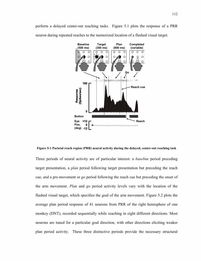
112
perform a delayed center-out reaching tasks. Figure 5.1 plots the response of a PRR
neuron during repeated reaches to the memorized location of a flashed visual target.
12deg
100sp/sRespo
nse
(Spi
kes/
sec)
100
0
+120
-12
Res
pons
e (S
pike
s/se
c)100
0
+120
-12
ButtonEye Pos. (deg)
Baseline (500 ms)
Target (300 ms)
Plan (800 ms)
Completed (variable)
Reach cue
Reach
Go
Figure 5-1 Parietal reach region (PRR) neural activity during the delayed, center-out reaching task
Three periods of neural activity are of particular interest: a baseline period preceding
target presentation, a plan period following target presentation but preceding the reach
cue, and a pre-movement or go period following the reach cue but preceding the onset of
the arm movement. Plan and go period activity levels vary with the location of the
flashed visual target, which specifies the goal of the arm movement. Figure 5.2 plots the
average plan period response of 41 neurons from PRR of the right hemisphere of one
monkey (DNT), recorded sequentially while reaching in eight different directions. Most
neurons are tuned for a particular goal direction, with other directions eliciting weaker
plan period activity. These three distinctive periods provide the necessary structural

113
information on the reach movement sequence. This information is especially important
for a prosthetic system that relies heavily on the control signals extracted from the neural
activities. Proper knowledge of these cognitive states not only provides extra control
parameters for practical implementation of the prosthetic devices, but also reveals how
PRR prepares and reacts to a reach movement.
In order to construct a robust autonomous prosthetic system, we also define the following
objects. The direction classifier uses spike data from the past 500 ms to estimate the
probability that a reach is being planned to each of the eight directions, and the most
probable reach direction is then selected. The period classifier uses spike data from the
past 250 ms to estimate the probability that PRR is currently in a baseline, plan or go
period (see Figure 5.1), and then the most probable class is selected using the Bayesian
classifier. Finally the interpreter takes in the series of baseline, plan and go
classifications, generated by the period classifier as time evolves, and determines when a
reach should be executed. It must also take in where the reach should be directed from
the direction classifier and finally issue the high-level control signal stating: reach here,
reach now.
Having introduced the concepts of period, period classifier, and direction classifier, we
now focus on the function and operation of the interpreter (Figure 5.2C).
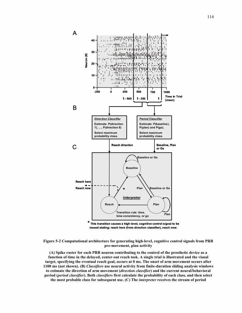
114
-250 0 250 500 750 1000Time in Trial (msec)
Period Classifier
Estimate: P(baseline), P(plan) and P(go).
Select maximum probability class.
tt - 250t - 500
Baseline
Plan
Plan
Transition rule: time,time-consistency, or go
A
B
C
Neur
on (#
)
10
20
30
40
0
Direction Classifier
Estimate: P(direction1), …, P(direction 8)
Select maximum probability class.
Baseline or Go
Baseline or Go
Baseline, Plan or Go
Reach
Reach direction
Interpreter
*
* This transition causes a high-level, cognitive control signal to be issued stating: reach here (from direction classifier), reach now.
Plan
Reach here
Reach now
Figure 5-2 Computational architecture for generating high-level, cognitive control signals from PRR pre-movement, plan activity
(A) Spike raster for each PRR neuron contributing to the control of the prosthetic device as a function of time in the delayed, center-out reach task. A single trial is illustrated and the visual
target, specifying the eventual reach goal, occurs at 0 ms. The onset of arm movement occurs after 1100 ms (not shown). (B) Classifiers use neural activity from finite-duration sliding analysis windows
to estimate the direction of arm movement (direction classifier) and the current neural/behavioral period (period classifier). Both classifiers first calculate the probability of each class, and then select
the most probable class for subsequent use. (C) The interpreter receives the stream of period

115
classifications (i.e., baseline, plan or go) from the period classifier and the stream of real direction classifications (e.g., downward reach) from the direction classifier. The interpreter consists of a finite
state machine that transitions among three states (baseline, plan and reach) according to some transition rules.
Again, the first function the interpreter must perform is to determine when a reach should
be executed given the series of baseline, plan and go classifications from the period
classifier. We implemented the interpreter with a finite state machine consisting of three
states: baseline, plan and reach. Importantly, although these states have similar labels to,
and have certain relationships with, the period classifier outputs (i.e., baseline, plan and
go period classifications) they are distinct. The period classifications govern, in part, the
transitions between states.
The interpreter starts in the baseline state and, as shown in Figure 5.2C, can transition to
the plan state or return to the baseline state each time the period classifier issues another
period classification. A baseline or go period classification keeps the interpreter in the
baseline state, while a plan period classification advances the interpreter to the plan state.
Once in the plan state, a baseline- or go-period classification will return the interpreter to
the baseline state. The reason for this operating logic will become clear when we discuss
below the possible rules for transitioning the interpreter from the plan state to the reach
state. Once the reach state is achieved the interpreter automatically transitions back to the
baseline state, and simultaneously issues a high-level, cognitive control signal
commanding an immediate reach to the location given by the goal classifier (Figure
5.2C, asterisk).

116
The question of when to transition the interpreter from the plan state to the reach state,
and subsequently triggering an arm movement, can be answered by considering the
behavioral task instructions and go period classifications. We now summarize the logic of
three different transition rules, as well as the results we obtained using these rules, to
show how increasingly sophisticated rules can potentially improve prosthesis control
performance.
1. Time transition rule. If the behavioral task instruction to the subject is simply “plan a
reach to a particular location for half a second,” then a prosthetic system can safely
execute an arm movement after detecting 500 ms of plan activity. In other words, the
interpreter can transition from the plan state to the reach state when the period classifier
issues 500 ms of contiguous plan classifications. Importantly, with this strategy the
subject could abort an arm movement by ceasing to plan at any time before 500 ms or
shift the reach target by simply changing his/her planned reach location before 500 ms
has passed. We term this the “time” transition rule. While this is the typical behavior
with the time criterion transition rule, particularly with large neuron populations and for
reaches to particular locations, this rule can error by failing to transition to the reach state
before the end of the trial’s experimental data or by executing a reach to the wrong goal
location.
The interpreter begins in the baseline state and correctly stays in the baseline state during
the phasic-response period mentioned previously (~100-400 ms following target
presentation). This is because the erroneous go period classification occurs after only a

117
brief period (less than 500 ms) of plan. The interpreter then correctly enters the plan state
and remains in this state, as long as the period classifier issues plan period classifications,
until the minimum length of continuous plan classification (500 ms) is surpassed causing
a transition to the reach state.
2. Time-consistency transition rule. A simple extension of the prior transition rule can
address these concerns by adopting the conservative view that it is better not to execute a
reach at all than to reach in the wrong direction. By adding the constraint that the period
classifier’s plan classifications must also specify a given goal direction throughout the
required plan period (500 ms) we effectively impose a plan-stability requirement. We
term this the “time-consistency” transition rule. Importantly, the period classifier, which
employs a 250 ms sliding window, can also estimate goal location using response models
and estimation methods analogous to those in the familiar direction classifier.
3. Go transition rule. While the previous two transition rules perform well for certain
applications, and importantly they do not rely on neural signals associated with
movement execution, we would also like to be able to produce a larger absolute number
of correct reaches. We can achieve this by replacing the previous stability constraint with
a requirement that the period classifier issue a go period classification, after plan period
classifications have been issued continuously for 500 ms, in order to transition from the
plan state to the reach state. We term this the “go” transition rule. Using a neural “go
signal” could afford the subject an additional opportunity to abort a planned reach by
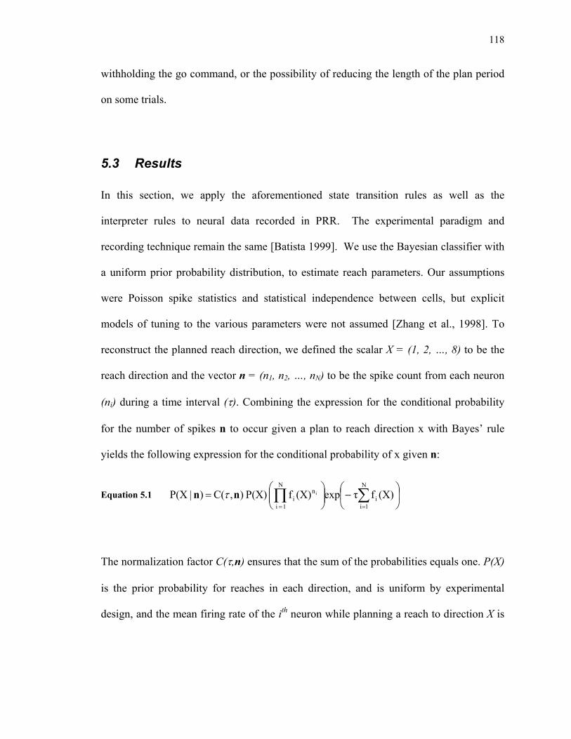
118
withholding the go command, or the possibility of reducing the length of the plan period
on some trials.
5.3 Results
In this section, we apply the aforementioned state transition rules as well as the
interpreter rules to neural data recorded in PRR. The experimental paradigm and
recording technique remain the same [Batista 1999]. We use the Bayesian classifier with
a uniform prior probability distribution, to estimate reach parameters. Our assumptions
were Poisson spike statistics and statistical independence between cells, but explicit
models of tuning to the various parameters were not assumed [Zhang et al., 1998]. To
reconstruct the planned reach direction, we defined the scalar X = (1, 2, …, 8) to be the
reach direction and the vector n = (n1, n2, …, nN) to be the spike count from each neuron
(ni) during a time interval (τ). Combining the expression for the conditional probability
for the number of spikes n to occur given a plan to reach direction x with Bayes’ rule
yields the following expression for the conditional probability of x given n:
Equation 5.1
−
= ∑∏
==
N
1ii
N
1 i
ni (X)fτexp(X)f P(X) ),C( )|P(X inn τ
The normalization factor C(τ,n) ensures that the sum of the probabilities equals one. P(X)
is the prior probability for reaches in each direction, and is uniform by experimental
design, and the mean firing rate of the ith neuron while planning a reach to direction X is

119
fi(x). The estimated reach direction, ∧
X , was taken to be the one with the highest
probability.
( )( )n|XPargmax{1,2,...8}X∈
∧
=X
A similar procedure was used to estimate the response distributions for the time-course
analyses, but with the following variations. After selection of the random subset of cells
and the exclusion of a single random trial from each cell, the remaining trials were
divided into 3 epochs: baseline, plan period, and pre-execution period (-600 to 0, 300 to
1000, and 1100 to 1350, respectively). The trials from each direction, for each cell, and in
each epoch were concatenated, and the data were sampled with 250ms long moving
windows with 50ms time steps. The baseline epoch was concatenated across all
directions. Additionally the plan epoch was also sampled using 500ms windows rather
than 250 ms windows. The mean of each epoch was used as the parameter for the single
multidimensional Poisson distribution for the baseline period, and for each of the 8
multidimensional distributions for each direction in the 3 other epochs (the 250ms
sampled memory epoch, the 500ms sampled memory epoch and the pre-execution
period). Test-data firing rates were measured in 250ms windows, advanced 50 ms at
each time step, through the duration of the test trial. The most probable condition
(baseline, one of 8 plan directions, or one of 8 execution directions) was estimated
independently in each time step as above. The direct results of this classification process
are shown in Figure 5.3.
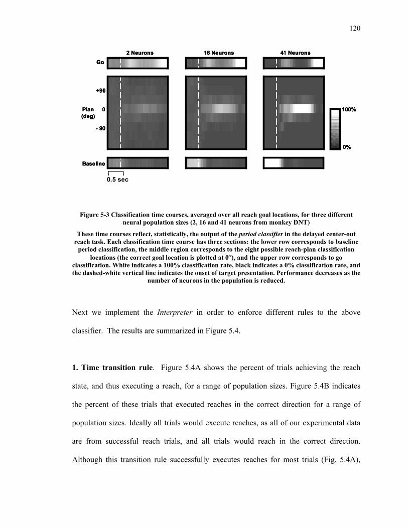
120
2 Neurons 16 Neurons 41 NeuronsGo
Baseline
Plan(deg)
0
+90
- 90
1 sec
0%
100%
0.5 sec
2 Neurons 16 Neurons 41 NeuronsGo
Baseline
Plan(deg)
0
+90
- 90
1 sec
0%
100%
2 Neurons 16 Neurons 41 NeuronsGo
Baseline
Plan(deg)
0
+90
- 90
1 sec
0%
100%
0.5 sec
Figure 5-3 Classification time courses, averaged over all reach goal locations, for three different neural population sizes (2, 16 and 41 neurons from monkey DNT)
These time courses reflect, statistically, the output of the period classifier in the delayed center-out reach task. Each classification time course has three sections: the lower row corresponds to baseline
period classification, the middle region corresponds to the eight possible reach-plan classification locations (the correct goal location is plotted at 0°), and the upper row corresponds to go
classification. White indicates a 100% classification rate, black indicates a 0% classification rate, and the dashed-white vertical line indicates the onset of target presentation. Performance decreases as the
number of neurons in the population is reduced.
Next we implement the Interpreter in order to enforce different rules to the above
classifier. The results are summarized in Figure 5.4.
1. Time transition rule. Figure 5.4A shows the percent of trials achieving the reach
state, and thus executing a reach, for a range of population sizes. Figure 5.4B indicates
the percent of these trials that executed reaches in the correct direction for a range of
population sizes. Ideally all trials would execute reaches, as all of our experimental data
are from successful reach trials, and all trials would reach in the correct direction.
Although this transition rule successfully executes reaches for most trials (Fig. 5.4A),

121
many of the reaches go in the wrong direction (Fig. 5.4B). These errors are due to
direction classifier miss-classifications, and are most likely caused by low signal to noise
ratios. If errors were caused by drifts in plan or volition then the prediction accuracy
would not be expected to increase dramatically by adding more neurons to the estimate.
2. Time-consistency transition rule. Figure 5.4 also summarizes the performance of
this transition rule. As expected, fewer trials now execute reaches (Fig. 5.4A) but those
that do tend to reach in the correct direction more often (Fig. 5.4B).
3. Go transition rule. Figure 5.4 illustrates the performance. The period of time used by
the direction classifier to estimate the reach direction, which is the 500 ms directly
preceding the go period classification, tends to be slightly later than with the previous
two transition rules. This is because the go period classification can occur up to several
hundred milliseconds after the plan duration criterion has been met. This accounts for the
increased percentage of reaches to the correct location (Fig. 5.4B). This algorithm
executes an intermediate number of reaches, as compared to the other two transition rules
(Fig. 5.4A), with good performance arising from the readily detected and classified go
activity.
A
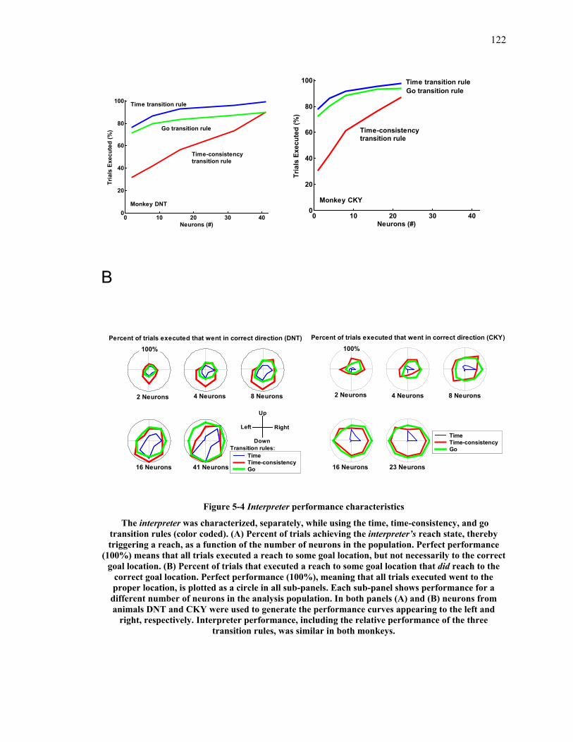
122
0 10 20 30 400
20
40
60
80
100
Neurons (#)
Tria
ls E
xecu
ted
(%)
Time transition rule
Go transition rule
Time-consistencytransition rule
Monkey DNT
0 10 20 30 400
20
40
60
80
100
Neurons (#)
Tria
ls E
xecu
ted
(%)
Time-consistencytransition rule
Go transition ruleTime transition rule
Monkey CKY
B
TimeTime-consistencyGo
2 Neurons 4 Neurons 8 Neurons
16 Neurons 41 Neurons
Up
Down
Left Right
100%Percent of trials executed that went in correct direction (DNT)
Transition rules:
TimeTime-consistencyGo
2 Neurons 4 Neurons 8 Neurons
16 Neurons 23 Neurons
100%Percent of trials executed that went in correct direction (CKY)
Figure 5-4 Interpreter performance characteristics The interpreter was characterized, separately, while using the time, time-consistency, and go
transition rules (color coded). (A) Percent of trials achieving the interpreter’s reach state, thereby triggering a reach, as a function of the number of neurons in the population. Perfect performance
(100%) means that all trials executed a reach to some goal location, but not necessarily to the correct goal location. (B) Percent of trials that executed a reach to some goal location that did reach to the
correct goal location. Perfect performance (100%), meaning that all trials executed went to the proper location, is plotted as a circle in all sub-panels. Each sub-panel shows performance for a
different number of neurons in the analysis population. In both panels (A) and (B) neurons from animals DNT and CKY were used to generate the performance curves appearing to the left and
right, respectively. Interpreter performance, including the relative performance of the three transition rules, was similar in both monkeys.

123
5.4 Conclusion
Although decoding stimulus and behavior parameters have been in existence for many
years, there does not yet exist a neural-prosthetic architecture that is optimal for all
plausible prosthetic applications. To explore the feasibility of using pre-movement
neural signals from PRR to generate high-level cognitive control signals, a computational
architecture is developed and tested in this chapter. This part of an envisioned neural
prosthetic system estimates, from PRR neural activity, when an arm movement is being
planned (period classifier), the direction of the planned movement (direction classifier),
and when the arm should move (interpreter). The resulting computations issue a
cognitive control signal with two parts: reach here and reach now. Thus using the neural
signal from PRR, it is sufficient to extract the necessary control signals for operating a
neural prosthetic. This structured decoding approach offers a first look at the possibility
of building an autonomous prosthetic device based completely on the information in the
neural data.

124
Chapter 6 Conclusion
Inspired by the considerable success of cochlear implants, tremor-control devices and
other neural-prosthetic systems aimed at delivering signals to the nervous system,
research aimed at reading out neural signals for prosthetics applications has intensified in
recent years. While the concept of translating neural activity from the brain into control
signals for prosthetic systems has existed for decades, substantial progress toward
realizing such systems has been made only relatively recently. This progress has been
fueled by advances in our understanding of neural coding, as well as by advances in
forming stable electrical interfaces with neurons and computational technologies for
processing neural signals in real time.
One interesting application of the neural prosthetic system is a prosthetic arm that is
connected directly to motor or pre-motor area of the brain. This allows direct control of
the prosthetic arm by mere thoughts of the user. In other words, one can control
peripheral devices just by thinking where to reach. Such a system could be especially
important for many locked-in patients or severe spinal cord injury sufferers [Katz 1992].
In addition, successful construction of this system should also shed light on the
underlying neural coding of the behavior parameters.
As this endeavor spans many different disciplines and research subjects, this thesis in
particular focuses on obtaining the necessary control signals for a prosthetic system such
as reach directions and cognitive states. In Chapter 3, a novel approach to characterize
spike trains is proposed. This approach determines the Poisson-ness of a spike train at
125
different scales while taking advantage of the multi-scale capability of wavelet packets, a
relatively new signal processing technique. Under this approach, the spike trains are
projected onto wavelet packets and the distributions of the projection coefficients are
analyzed. It allows us to assess Poisson-ness from different scales. The Poisson-ness is
an especially important quantity for decoding because if the spike train is indeed Poisson
in nature, then the ubiquitous mean firing rate measure is the only relevant feature.
As seen from the examples of Chapter 3, not all neurons exhibit a Poisson nature.
Therefore, it is necessary to devise a method that searches for the most discriminating
feature(s) towards decoding. Chapter 4 first uses the Haar wavelet packet to construct a
naïve feature set. Because of the time domain properties of the Haar wavelet packet
functions, these features have intuitive biological interpretations that are appealing to
researchers in the neuroscience community. Then of all the features, the most
informative ones are selected using an optimal feature search technique. The technique
prunes the wavelet packet tree while using mutual information as a score function to rank
the decodability of each feature. When combined with the Bayesian classifier, this
method returns improved decoding performance versus approaches based on the firing
rate. The method was tested on both artificial data and actual neuronal data from PRR,
and compared to mean firing rate decoding.
Besides decoding the estimated reach directions from PRR signals, additional cognitive
parameters are necessary for building an autonomous prosthetic device. For a minimally
autonomous robotic device, Chapter 5 defines the behavior states to include a baseline

126
state, reach planning states, and the reach execution go state. When combined with an
Interpreter that acts on the classification results of these states, it returns an efficient
algorithm that extracts the necessary cognitive control parameters. Experimental data
collected from PRR while the animal is performing a sequence of actions are subjected to
this method while we compare different state transition rules.
Although the work in this thesis largely focuses on decoding discrete stimulus parameters
from spike data, the decoding framework and technique can be extended to other types of
signals such as LFP and EEG. In addition, it is possible that more complicated trajectory
decoding problem may be cast in the discrete parameter problems as well because studies
have shown that PRR encodes the next movement target. Therefore, it is conceivable that
one can discretize a trajectory into a set of sequential movement targets though further
experiments and studies are necessary to validate this suggested approach.
127
Bibliography A Abbott, L.F., Decoding neuronal firing and modeling neural networks, Quarterly Review of Biophysics, 27:291-331 (1994) Alur, R. and D.L. Dill, A Theory of Timed Automata, Theoretical Computer Science No. 126, pp183-235, 1994 Brandin, B. and W.M. Wonham, Supervisory control of timed discrete event systems, IEEE Transactions on Automatic Control, Vol. 39, No. 2, pp 329-342, 1994 Abeles, A. and M. Goldstein, Multispike Train Analysis, Proceedings of the IEEE, vol. 65, pp 762-773, 1977 Andersen, R.A., L.H. Snyder, D.C. Bradley, and J. Xing, Multimodal representation of space in the posterior parietal cortex and its use in planning movements, Annual Review of Neuroscience, 20:303-330, 1997 B Brown, E.N., L.M. Frank, D. Tang, M.C. Quirk, M.A. Wilson, A statistical paradigm for neural spike train decoding applied to position prediction from ensemble firing patterns of rat hippocampal place cells, Journal of Neuroscience, Sept. 15; 18(18): 7411-25, 1998 Batista, A.P., C.A. Buneo, L.H. Snyder and RA Andersen, Reach plans in eye-centered coordinates, Science, 285:257-260, 1999 Batista, A.P., and Andersen, R.A., The parietal reach region codes the next planned movement in a sequential reach task, Journal of Neurophysiology, 85:539-544, 2001 Brandman, R. and M.E. Nelson, A simple model of long-term spike train regularization, Neural Computation, 14:1575-1597, 2002 C Cherkassky, V. and F. Mulier, Learning from Data - Concepts, Theory and Methods, Wiley, New York, 1998 Cover, T. and J. Thomas, Elements of Information Theory, Wiley, New York, 1991 Cassandras, C. and S. Lafortune, Introduction to Discrete Event Systems, Kluwer Academic Publishers (Norwell, MA), 1999 D Daubechies, I., Ten Lectures on Wavelets, SIAM, Philadelphia, PA, 1992
128
Devroye, L, L. Gyorfi, and G. Lugosi, A Probabilistic Theory of Pattern Recognition, Springer Verlag, 1996. Donoghue J.P., Connecting cortex to machines: recent advances in brain interfaces. Nature Neuroscience 5 Supplement: 1085 – 1088, 2002 Donoho, D.L., & I.M. Johnstone, Ideal denoising in an orthonormal basis chosen from a library of bases. Compt. Rend. Acad. Sci. Paris Ser. A, 319, 1317-1322, 1994 E F Fisher R.A., The use of multiple measurements in taxonomic problems. Annals of Eugenics 7, pages 179-188, 1936 Florence, S.L., H.B. Taub, and J.H. Kaas, Large-scale sprouting of cortical connections after peripheral injury in adult macaque monkeys, Science, 282(5391): p. 1117-1121, 1998 G Georgopoulos, A.P., A. Schwartz, and R.E. Kettner, Neuronal population coding of movement direction, Science, 233:1416-1419, 1986 Georgopoulos A.P., R.E. Kettner, and A Schwartz, Primate motor cortex and free arm movements to visual targets in three-dimensional space, II, Coding of the direction of movement by a neuronal population, Journal of Neuroscience 8:2928-2937, 1988 Gabbiani, F. and C. Koch, Principles of Spike Train Analysis Methods in Neuronal Modeling: From Synapses to Networks, C Koch and I Segev, eds., 2. edition, . MIT Press: Cambridge, MA 0:313-360, 1998 Greenwood, P., A Guide to Chi-Squared Testing, Wiley, NY, 1996. H Humphrey, D.R., Electrophysiological Techniques, Society for Neuroscience, Atlanta, 1979 I Isaacs, R., D. Weber and A. Schwartz, Work toward real-time control of a cortical prothesis, IEEE Trans. Rehabil. Eng. 8:196-198, 2000 J Jelinek, F., Statistical Methods for Speech Recognition, MIT Press, Cambridge MA, 1998 Johnson, D.H. and R.M. Glantz, When does interval coding occur? CNS, 2003
129
Johnson D.H., C.M. Gruner, K. Baggerly, and C. Seshagiri, Information-theoretic analysis of neural coding, Journal of Computational Neuroscience, 10:47-69, 2001 Johnson D.H., Point process models of single-neuron discharges. Journal of Computational Neuroscience, 3:275-299, 1996 Johnson, P.B., S. Ferraina, L. Bianchi, and R. Caminiti, Cortical networks for visual reaching: physiological and anatomical organization of frontal and parietal lobe arm regions. Cerebral Cortex, 6:102-119, 1996 K Kralik J.D., D.F. Dimitrov, D.J. Krupa, D.B. Katz, D. Cohen, and A.L. Nicolelis, Techniques for long-term multisite neuronal ensemble recordings in behaving animals, Methods 25, 121-150, 2001 Kaas, J.H., Sensory loss and cortical reorganization in mature primates, Progress in Brain Research, 138: p. 167-176, 2002 Katz, R.T., Long-Term survival, prognosis, and life-care planning for 29 patients with chronic locked-in syndrome, Arch. of Physical Medicine and Rehabilitation, 73(5): p. 403-408, 1992 Kolaczyk, E.D., Non-parametric estimation of Gamma-ray burst intensities using Haar wavelets, The Astrophysical Journal, Vol. 483, 340-349, 1997 Kennedy, P.R., R.A.E. Bakay, M.M. Moore, K. Adams, and J. Goldwaithe, Direct control of a computer from the human central nervous system, IEEE Transactions on Rehabilitation Engineering 8, 198-202, 2000 L Learned, R. and A.S. Willsky, A wavelet packet approach to transient signal classification, Applied and Computational Harmonic Analysis 2, 265-278, 1995 Lewicki, M.S., A review of methods for spike sorting: the detection and classification of neural action potentials, Network: Computation in Neural Systems 9(4): R53-R78, 1998 M Moran, D.W. and A.B. Schwartz, Motor cortical representation of speed and direction during reaching, Journal of Neurophysiol 82(5): 2676-2692, 1999 Mallat, S., A Wavelet Tour of Signal Processing, Academic Press; 2nd edition, 1999 Mallat, S., G. Papanicolaou, and Z. Zhang, Adaptive covariance estimation of locally stationary processes, Annals of Statistics, vol. 26, no. 1, 1998
130
Meeker, D., K.V. Shenoy, S. Cao, B. Pesaran, H. Scherberger, M. Jarvis, C.A. Buneo, A.P. Batista, S.A. Kureshi, P.P. Mitra, J.W. Burdick, RA Andersen, Cognitive control signals for prosthetic systems. Society For Neuroscience 27, 2001 Meeker D., K.V. Shenoy, S. Kureshi, S. Cao, J. Burdick, B. Pesaran, P. Mitra, A. Batista, C. Buneo, B. Gillikin, D. Dubowitz, R.A. Andersen, Toward adaptive control of neural prosthetics by parietal cortex. Neural Information and Coding Workshop, 2000 Meeker, D. and R.A. Andersen, Rapid plasticity in the parietal reach region demonstrated with a brain-computer interface, Society For Neuroscience. 29, 2003 N Nicolelis, M., The amazing adventures of robotrat, Trends in Cognitive Sciences 6: 449-450, 2002 Nicolelis, M., Actions from thoughts, Nature, 409:403-407, 2001 Nowak, R., Multiscale Hidden Markov Models for Bayesian Image Analysis, Bayesian Inference in Wavelet Based Models, Springer-Verlag, 1999 Nenadic Z. and J.W. Burdick, Spike detection using continuous wavelet transform, manuscript in preparation, 2003 O Oppenheim, A.V. and R.W. Schafer, Digital Signal Processing, Prentice-Hall, Englewood Cliffs, NJ, 1975 Oweiss, K.G., Multiresolution analysis of multichannel neural recordings in the context of signal detection, estimation, classification and noise suppression, Ph.D. Thesis, University of Michigan, Ann Arbor, May 2002 Oweiss, K.G. and D.J. Anderson, Noise Reduction in Multichannel Neural Recordings using a new array wavelet denoising algorithm, Neurocomputing, vol 38-40, pp.1687-1693, 2001 P Parzen, E., On the estimation of probability density function and the mode, The Analysis of Mathematical Statistics 33, 1965 Percival, D.B. and A.T. Walden, Wavelet Methods for Time Series Analysis, Cambridge University Press, 2000 Q R
131
Ross S.M., Stochastic Processes, Wiley, New York, NY, 1994 Ross S.M., Introduction to Probability and Statistics for Engineers and Scientists, Wiley, New York, 2000 Reich, D.S., F. Mechler, K.P. Purpura, and J.D. Victor, Interspike intervals, recepive fields and information coding in primary visual cortex, Journal of Neuroscience, 20:1964-1975, 2000 Rabiner, L.R., A tutorial on hidden Markov models and selected applications in speech recognition, Proceedings of the IEEE, vol. 37 no. 2 pp57-86, 1989 S Shannon, C.E. and W. Weaver, The Mathematical Theory of Communication, University of Illinois Press, Urbana, IL, 1959 Schwartz, A.B. and D.W. Moran, Arm trajectory and representation of movement processing in motor cortical activity, European Journal of Neuroscience 12(6):1851-1856, 2000 Schwartz A.B., R.E. Kettner, and A.P. Georgopoulos, Primate motor cortex and free arm movements to visual targets in three-dimensional space I. Relations between single cell discharge and direction of movement, Neuroscience 8:2913-2927, 1988 Steveninck, R., G. Lewen, S.P. Strong, R. Koberle, and W.A. Bialek, Reproducibility and variability in neural spike trains, Science 275: 1805-1808, 2002 Sanger, T.D., Probability density estimation for the interpretation of neural population codes, Journal of Neurophysiology, 76(4):2790--2793. 11, 1996 Savage, J., Models of Computation, Addison-Wesley, Reading MA, 1989 Snyder, L.H., A.P. Batista, and R.A. Andersen, Coding of intention in the posterior parietal cortex, Nature, 386:167-169, 1997 Shenoy, K.V., D. Meeker, S. Cao, S.A. Kureshi, C.A. Buneo, A.P. Batista, J.W. Burdick, R.A. Andersen, Toward prosthetic systems controlled by parietal cortex. Neural Information and Coding Workshop, 2001 Shenoy, K.V., D. Meeker, S. Cao, S.A. Kureshi, B. Pesaran, C.A. Buneo, A.P. Batista, P.P. Mitra, J.W. Burdick, and R.A. Andersen, Neural prosthetic control signals from plan activity, NeuroReport, 14:591-596, 2003. Strong, S.P., R. Koberle, R. Steveninck and W. Bialek, Entropy and Information in Neural Spike Trains, Physical Review Letters 80:197-201, 1998
132
Saito N., R.R. Coifman, F.B. Geshwind, and F. Warner, Discriminant feature extraction using empirical probability density estimation and a local basis library, Pattern Recognition, vol. 35, pp.2841-2852, 2002 T Teich, M.C. and S.M. Khanna, Pluse-number distribution for the neural spike train in the cat’s auditory nerve, Journal of Acoustic Society of America. 77:1110-1128, 1985 Stirzaker, D., Elementary Probability, Cambridge University Press, 1994 U V Viterbi, A.J., Error bounds for convolutional codes and an asymmetrically optimum decoding algorithm, IEEE Transactions on Information Theory, vol. IT-13 pp.260-67, 1967 Victor, J.D. and K.P. Purpura, Metric-space analysis of spike trains: theory, algorithms and application, Network: Computation in Neural Systems 8: 127—164, 1997 Vapnik, V., The Nature of Statistical Learning Theory, Springer, Berlin, 1995 W Wessberg, J., C. Stambaugh, J. Kralik, P. Beck, M. Laubach, J. Chapin, J. Kim, S. Biggs, M. Srinivasan, and M. Nicolelis, Real-time prediction of hand trajectory by ensembles of cortical neurons in primates, Nature, 408(6810):361-5, 2000 Wickerhauser, M.V., Adapted Wavelet Analysis from Theory to Software, Wellesley, MA, 1994 Wolpert, D.M. and Z. Ghahramani, Computational principles of movement neuroscience. Nature Neuroscience. 3:1212-1217, 2001 X Y Z Zhang, K., I. Ginzburg, B.L. McNaughton, and TJ Sejnowski, Interpreting Neuronal Population Activity by Reconstruction, The American Physiological Society, pp. 1017-1044, 1998.
133
Appendix 1: Proof of Proposition 3.1
The proof of this proposition proceeds by induction.
Step 1: First consider the scale j = 1. The wavelet packet coefficients Tvvv 00201 ,...,, at
scale 0 are independent because of the independent increments property P1. By
construction from the Pyramid Algorithm, we know that the child coefficients at scale j=1
are
kkTk
kkk
vvvvvv
2,012,02
,1
2,012,0,1
−=
+=
−+
−
, for 2
,...,2,1 Tk =
Thus the joint probability between any coefficients 1211 ,vv can be written as,
∑∑
∑∑
∑
−==−===
−==−==−===
=+=+−===
=+=+=+=++=
yx
y x
x
yvvyvPxvvxvP
yvvyvPyvvyvxvvxvP
vvvPvvvxvvxvPvvvPvvvvvvP
vvvvPvvP
)',(),(
)',()',|,(
)'()'|,()'()'|(
),(),(
04030201
040304030201
040304030201
040304030201
040302011211
The last equality is due to the independence given by property P2. Here x and y describe
the range of the coefficients at scale j=1, where Range(v1k) = {-1 0 1}. Continuing, we
have:
)()()'()(),(
1211
040302011211
vPvPvvvPvvvPvvP
==+=+=
where the last step is a consequence of the parent-child relationship in the Pyramid
algorithm. We can generalize the above result to all the members of the low pass child to

134
show that all the coefficients 2
11211 ,...,, Tvvv are mutually independent. Similarly, we can
show the independence between all the members of the coefficients related to the high
pass child TTT vvv 1)22
(1)12
(1,...,,
++ .
Step 2: To establish the induction, consider the wavelet packets and their coefficients at
scale j = j*. Assume all the coefficients
{ } *
*
*2
)1(
21
j
j
Tl
Tlkkjv+
+=, 1*
2,...,1,0 −= jl
at each node are mutually independent. We know from Step 1 that this is true for j*=1.
Step 3: To proceed with the induction, assume the mutual independence of coefficients
at scale j*. Now consider scale j*+1. Using the same approach as step 1 of the proof, at
scale j = j*+1 the coefficients associated with the low pass child node branched from the
parent node at scale j* have the following joint distribution,
)()()'()(
)',(),(
)',()',|,(
)'()'|,(
)'()'|(
),(
),(
2)1(1)1(4321
4321
434321
434321
434321
4321
2)1(1)1(
******
****
******
******
******
****
**
++
++
==+=+=
−==−===
−==−==−===
=+=+−===
=+=+=+=
++=
∑∑
∑∑
∑
jjjjjj
yjjjj
x
jjy
jjjjx
jjjjjjx
jjjjjj
jjjj
jj
vPvPvvvPvvvP
yvvyvPxvvxvP
yvvyvPyvvyvxvvxvP
vvvPvvvxvvxvP
vvvPvvvvvvP
vvvvP
vvP

135
We can further generalize the above result to all the members of the low pass child so
that the set of coefficients { } 1*
1*
*2
)1(
21)1(
+
+
+
+=+
j
j
Tl
Tlkkjv , *
2,...,1,0 jl = are all mutually independent.
Similarly, we can show the independence between all the members of the high pass child
of the parent node at scale j*. Therefore, we have proven that the members of any child
node, namely the leaf of the wavelet packet tree, are independent.
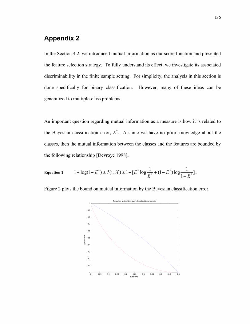
136
Appendix 2
In the Section 4.2, we introduced mutual information as our score function and presented
the feature selection strategy. To fully understand its effect, we investigate its associated
discriminability in the finite sample setting. For simplicity, the analysis in this section is
done specifically for binary classification. However, many of these ideas can be
generalized to multiple-class problems.
An important question regarding mutual information as a measure is how it is related to
the Bayesian classification error, E*. Assume we have no prior knowledge about the
classes, then the mutual information between the classes and the features are bounded by
the following relationship [Devroye 1998],
Equation 2 ]1
1log)1(1log[1);()1log(1 **
***
EE
EEXvIE
−−+−≥≥−+ .
Figure 2 plots the bound on mutual information by the Bayesian classification error.
0 0.05 0.1 0.15 0.2 0.25 0.3 0.35 0.4 0.45 0.50
0.1
0.2
0.3
0.4
0.5
0.6
0.7
0.8
0.9
1
Error rate
Mutual Info
Bound on Mutual info given classification error rate
137
Figure A.0-1 Mutual information bounded by the Bayesian classification error E*.
The red line corresponds to the lower bound and the blue line corresponds to the upper bound. X-axis is the error rate E*and y-axis marks the mutual information
Evidently, large mutual information corresponds to a smaller classification error. Notice
the bound is somewhat loose, i.e. a large range of mutual information can correspond to
the same classification error. Then why does mutual information work well as a
discriminability measure?
To address this question, E* is first re-examined. Recall Equation 4, the classification
error is defined as
{ } )()|0(),|1(min
)()|~(
)~(*
vPvXPvXP
vPvXXP
XXPE
v
v
∑
∑===
≠=
≠=
.
Using the Bayes’ rule, we can rewrite the above equation as,
{ }∑ ===v
XvPXvPE )0|(),1|(min21* ,
assuming the two classes are equally likely. With some algebraic manipulation, the
above equation is re-formulated as
Equation 3
∑
∑
−−=
−−+=
v
v
vPvP
vPvPvPvPE
)()(211
)()()]()([21
01
0101*
,
where for simplicity of notation, P1(v) and P0(v) replaces P(v|X=1) and P(v|X=0)
respectively. In addition, the term

138
Equation 4 ∑ −=v
Ko vPvPD )()( 01
is called the Kolmogrov divergence [Devroye 1998]. Further note that the Kolmogrov
divergence can be written as,
Equation 5 ∑ +−
⋅=v
Ko vPvPvPvP
vPD)()()()(
2)(21
21
01 ,
which can be interpreted as the expected value over v of the scaled absolute difference
between the two conditional probability distributions. Here, the scaling factor is
)(1
)()(2
21 vPvPvP=
+. Its effect will be explained in the following simple example.
Example: Consider two observed coefficients v1 and v2 where the absolute difference
between the conditional probability distributions is the same,
)()()()( 22211211 vPvPvPvP −=− .
In addition assume
)()( 21 vPvP > .
Therefore, we see that
)()()(
)()()(
2
2221
1
1211
vPvPvP
vPvPvP −
<−
.
This result makes practical sense because even the difference between the conditional
distributions is the same at v1 and v2, the classification error at v1 is greater than the one at
v2, i.e.
)()( 2*
1* vEvE > ,
where
139
)()()(
1)( 21*
vPvPvP
vE−
−=
the Bayesian classification error at v. Thus, )(
1vP
augments the difference between the
conditional distributions according to the classification error.
The above assertion assumes the conditional probabilities P1(v) and P2(v) are known a
priori, in which case the Kolmogrov divergence DKo as well as the classification E* can
be computed exactly. In practice however, one must estimate the conditional
probabilities from the observed training data. When the training data samples are limited,
the above calculation breaks down considerably. Consider the following simple case in
which v takes value 1 or 0 only, and the true conditional probabilities are
ββαα
−====−====
1)|0(,)|1(1)|0(,)|1(
22
11
XvPXvPXvPXvP
.
Therefore, for a training sample of size N, the probability of observing n1 1’s given class
X1 is
11 )1()|(1
11nNn
nN
XnSP −−
== αα ,
and similarly the probability of observing n2 1’s given class X2 is
22 )1()|(2
22nNn
nN
XnSP −−
== ββ ,
where S is a random variable such that
∑=
=N
iivS
1.
In addition, if we estimate the conditional probabilities using the histogram rule, i.e.
140
NnXvP
NnXvP
NnXvP
NnXvP
22
22
11
11
1)|0(,)|1(
1)|0(,)|1(
−====
−====
∧∧
∧∧
,
then the probability of obtaining these estimation becomes
11 )1()1)0(())1((1
11
11
nNn
nN
NnPP
NnPP −
∧∧
−
=−=== αα
and
22 )1()1)0(())1((2
22
22
nNn
nN
NnPP
NnPP −
∧∧
−
=−=== ββ ,
where ∧
1P and ∧
0P are two random variables representing the estimated probability
)|( 1XvP∧
and )|( 2XvP∧
, respectively. Because the above probabilities are nothing more
than binomial distributions, the expected value of the estimated probabilities are
ββ
αα
−=
=
−=
=
∧∧
∧∧
1)0(,)1(
1)0(,)1(
22
11
PEPE
PEPE,
and the variance of the estimated probabilities are
NPV
NPV
NPV
NPV
)1()0(,)1()1(
)1()0(,)1()1(
22
11
ββββ
αααα
−=
−
=
−=
−
=
∧∧
∧∧
.
Consequently, the variances associated with the sums and differences of the conditional
distributions are
141
NNPPV
NNPPV
)1()1()0()0(
)1()1()1()1(
21
21
ββαα
ββαα
−+
−=
−
−+
−=
−
∧∧
∧∧
,
and
NNPPV
NNPPV
)1()1()0()0(
)1()1()1()1(
21
21
ββαα
ββαα
−+
−=
+
−+
−=
+
∧∧
∧∧
.
Hence, the term )()()()(
21
01
vPvPvPvP
+− depends on the estimation of the conditional distributions.
And this dependence become substantial when )()( 01 vPvP − or )()( 01 vPvP + approaches
0. In another word, the Kolmogrov discriminability measure, DKo is overwhelmed by the
uncertainty at v if 0)()( 01 ≈− vPvP or 0)()( 01 ≈+ vPvP . Therefore, it is essential to trade
off the classification performance for robustness against such a finite sample effect.
In order to suppress the finite sample effect, it is necessary to become conservative when
interpreting the weighted difference between the conditional probability distributions,
namely )()()()(
21
01
vPvPvPvP
+− . First revisit the mutual information and manipulate it into the
following,
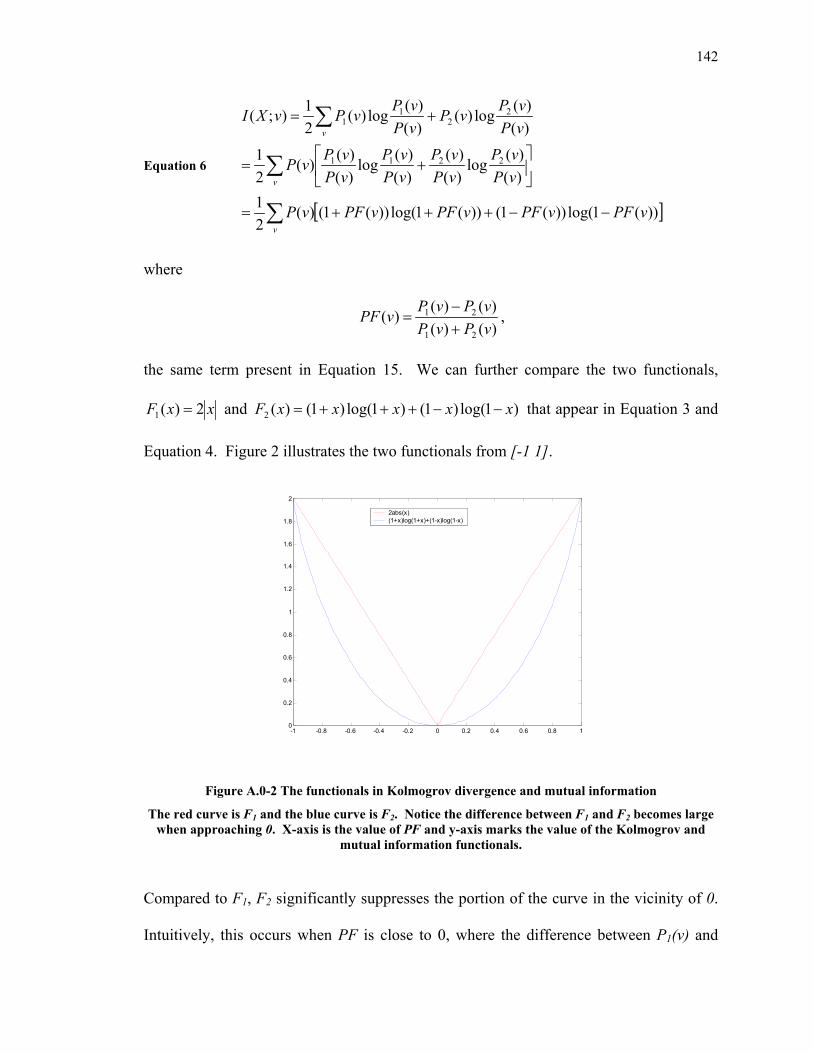
142
Equation 6
[ ]∑
∑
∑
−−+++=
+=
+=
v
v
v
vPFvPFvPFvPFvP
vPvP
vPvP
vPvP
vPvPvP
vPvPvP
vPvPvPvXI
))(1log())(1())(1log())(1()(21
)()(log
)()(
)()(log
)()()(
21
)()(log)(
)()(log)(
21);(
2211
22
11
where
)()()()()(
21
21
vPvPvPvPvPF
+−
= ,
the same term present in Equation 15. We can further compare the two functionals,
xxF 2)(1 = and )1log()1()1log()1()(2 xxxxxF −−+++= that appear in Equation 3 and
Equation 4. Figure 2 illustrates the two functionals from [-1 1].
-1 -0.8 -0.6 -0.4 -0.2 0 0.2 0.4 0.6 0.8 10
0.2
0.4
0.6
0.8
1
1.2
1.4
1.6
1.8
2
2abs(x)(1+x)log(1+x)+(1-x)log(1-x)
Figure A.0-2 The functionals in Kolmogrov divergence and mutual information
The red curve is F1 and the blue curve is F2. Notice the difference between F1 and F2 becomes large when approaching 0. X-axis is the value of PF and y-axis marks the value of the Kolmogrov and
mutual information functionals.
Compared to F1, F2 significantly suppresses the portion of the curve in the vicinity of 0.
Intuitively, this occurs when PF is close to 0, where the difference between P1(v) and

143
P2(v) is dominated by the variance of the estimation, an effect of finite training sample.
Therefore, using mutual information as the discriminability measure remains
conservative when the underlying probability estimation is dominated by uncertainty. By
doing so, the finite sample effect is also successfully suppressed. Hence, mutual
information effectively trades tightness of the error bound for robustness when dealing
with a finite number of samples.


![Entropy-based parametric estimation of spike train statistics … · 2013. 12. 8. · arXiv:1003.3157v2 [physics.data-an] 26 Aug 2010 Entropy-based parametric estimation of spike](https://img.pdfslide.us/doc/110x75/61267f632e04c272127aaf22/entropy-based-parametric-estimation-of-spike-train-statistics-2013-12-8-arxiv10033157v2.jpg)