BIOMEDICAL ENGINEERING

SPIKE TRAIN ANALYSIS OF SPATIAL DISCRIMINATIONS AND

FUNCTIONAL CONNECTIVITY OF PAIRS OF NEURONS

IN CAT STRIATE CORTEX

JASON MICHAEL SAMONDS

Thesis under the direction of Professor A. B. Bonds

We studied changes in ensemble responses of striate cortical pairs for small

(<10deg, 0.1c/deg) and large (>10deg, 0.1c/deg) differences in orientation and spatial

frequency. Examination of temporal resolution and discharge history revealed

advantages in discrimination from both dependent (connectivity) and independent

(bursting) interspike interval properties. We found the average synergy (information

greater than that summed from the individual neurons) was 50% for fine discrimination

of orientation and 25% for spatial frequency and <10% for gross discrimination of both

orientation and spatial frequency.

Dependency (Kullback-Leibler "distance" between the actual responses and two

wholly independent responses) was measured between pairs of neurons while varying

orientation, spatial frequency, and contrast. In general, dependency was more selective to

spatial parameters than was firing rate. Variation of dependence against spatial

frequency corresponded to variation of burst rate, and was even narrower than burst rate

tuning for orientation. We also found a gradual decline (adaptation) of dependency over

time that is faster for lower contrasts and which is likely a result of the decrease in

isolated (non-burst) spikes.

The results suggest that salient information is more strongly represented in bursts,

but that isolated spikes also have a role in transferring this information between neurons.

The dramatic influence of burst length modulation on both synaptic efficacy and

dependency around the peak orientation leads to substantial cooperation that can improve

discrimination in this region.

Approved___________________________________________ Date________________

SPIKE TRAIN ANALYSIS OF SPATIAL DISCRIMINATIONS AND

FUNCTIONAL CONNECTIVITY OF PAIRS OF NEURONS

IN CAT STRIATE CORTEX

By

Jason Michael Samonds

Thesis

Submitted to the Faculty of the

Graduate School of Vanderbilt University

in partial fulfillment of the requirements

for the degree of

MASTER OF SCIENCE

in

Biomedical Engineering

May, 2002

Nashville, Tennessee

Approved: Date:

ACKNOWLEDGEMENTS

I express my gratitude to Professor A. B. Bonds for his guidance and

encouragement throughout this project, as well as his support during my time at

Vanderbilt University. I would also like to extend my gratitude to Professor Don

Johnson for his assistance in explaining the finer details of type analysis, and to Professor

Jonathan Victor for sharing his knowledge and experience with spike train analysis. I am

very grateful to Professor Ross Snider for working with me in order to use his spike

sorting and cross-correlation software to contribute to my results. And lastly, I would

like to thank Dr. John Allison and Heather Brown for their help in collecting the data.

Although this project would not be possible without their assistance, all the ideas, type

analysis software, writing, and conclusions are my own work.

I would also like to thank the Graduate School and the National Institute of Health

(Grant RO1 EY03778) for providing financial support during my time in graduate school.

And it goes without saying that I am always grateful for the support from friends and

family that has always been there throughout my educational pursuits.

ii

TABLE OF CONTENTS

Page

ACKNOWLEDGEMENTS............................................................................................... ii

LIST OF FIGURES .......................................................................................................... iv Chapter I. NEURAL POPULATION ANALYSIS REVIEW........................................................ 1

Introduction............................................................................................................ 1 Theoretical Background............................................................................. 2 Single-unit Research .................................................................................. 6 Multi-unit Research ................................................................................. 10 Functional Imaging .................................................................................. 14

Correlation and Connectivity............................................................................... 15 Point Process and Cross-correlation ........................................................ 15 Partialization ............................................................................................ 19 Gravitational Clustering........................................................................... 19 Information Theory: Dependency and Complexity ................................. 21 Causality .................................................................................................. 22 Nonlinear Methods................................................................................... 23

Neural Code Theory............................................................................................. 24 Average Spike Rate Code ........................................................................ 25

Temporal Code......................................................................................... 26 Bursting....................................................................................... 27 Latency........................................................................................ 28 Spatiotemporal Patterns .............................................................. 30 Oscillations ................................................................................. 31 Chaos Theory ........................................................................................... 33

Information Theory............................................................................................. 35 The Future........................................................................................................... 39

II. COOPERATION BETWEEN AREA 17 NEURON PAIRS THAT ENHANCES FINE DISCRIMINATION OF ORIENTATION................................................................. 41

Introduction......................................................................................................... 41 Methods............................................................................................................... 44

Preparation ............................................................................................... 44 Stimuli...................................................................................................... 45 Data Acquisition and Spike Classification .............................................. 47

Type Analysis .......................................................................................... 48

iii

Results................................................................................................................. 53 Latency..................................................................................................... 55 Temporal Resolution................................................................................ 59 Discharge History .................................................................................... 63 Synergy, Independence, and Redundancy ............................................... 68 Confidence in Distance Estimations ........................................................ 73 Functional Connectivity........................................................................... 76

Discussion........................................................................................................... 87 Latency..................................................................................................... 87 Independent ISI Characteristics ............................................................... 89

Bursts and Connectivity........................................................................... 90 Functional Connectivity and Synergy...................................................... 92 Orientation Discrimination ...................................................................... 94

III. FUTURE EXPLORATIONS.................................................................................... 95

Introduction.......................................................................................................... 95 Cortical Function Theory..................................................................................... 96

Multidimensional Data....................................................................................... 100 Cortical Clustering ............................................................................................. 101 Spatiotemporal Connectivity ............................................................................. 103 REFERENCES .............................................................................................................. 105

iv

LIST OF FIGURES Figure Page 1. An example of firing rate tuning and fine and gross discriminations..................... 55 2. Enhanced discrimination with latency differences ................................................. 58 3. Distance rates versus temporal resolution............................................................... 62 4. Determination of Markov order of analysis............................................................ 64 5. Discharge history contribution to orientation discrimination ................................. 66 6. Discharge history contribution to spatial frequency discrimination ....................... 67 7. Ensemble distance versus individual neuron distances .......................................... 72 8. Distances and synergy versus random sample size................................................. 75 9. Another example of sample size functions ............................................................. 77 10. Temporal dynamics of dependnecy between neurons ............................................ 81 11. Difference between dependency and firing rate during contrast modulation ......... 83 12. Temporal dynamics of dependency adaptation....................................................... 84 13. Dependency tuning for orientation and spatial frequency modulation................... 86

v

CHAPTER I

NEURAL POPULATION ANALYSIS REVIEW

Introduction

One of the most elusive questions in biological sciences has been how the brain is

able to encode and decode the multi-dimensional features of sensory signals and to

formulate perceptions or perform actions on the order of hundreds of milliseconds. The

majority of neurophysiological studies have relied on counting the number of spikes

recorded from a single neuron and demonstrating how this spike count varies according

to sensory input features. Although these data represent the average response of only one

neuron to specific stimulus features, neurophysiologists have at the same time

acknowledged that the brain could only perform their complex operations with

populations of neurons. The brain cannot be thought of as simply as a passive screen

receiving a projected image of the outside world. The brain is able to separate figure

from background, perform invariant recognition, and make accurate and generalized

predictions. Understanding the representation of sensory information both on local and

global levels is equally important, and neither of these tasks presents a clear approach to

finding a solution. It cannot even be posed as a simple encoding and decoding problem

because there is not always a clear input and output.

In this introduction, we describe how the theories of brain function have evolved

over the last two centuries and how anatomical and physiological studies of individual

neurons and small groups of neurons have contributed to these theories. Then we

1

describe the methods that have been developed to analyze interactions between nerve

cells and when and how they are applicable to providing insight to cortical functions.

One of the difficulties in understanding brain function is deciding where to start the

analysis. We describe some of the theories of what aspects of the individual neuron's

signal carry the sensory information. Since we are looking at how information is

transmitted and manipulated in the brain, information theory has become an important

analytical tool. Lastly, we discuss where the theories of neural population codes might be

heading and how some of the conflicting arguments might be resolved.

Theoretical background

In a recent review, Doetsch (2000) points out that the idea that sensory

information was encoded in patterns of populations of neurons was proposed as early as

1802 by Young and elaborated by von Helmholtz in 1860 for explaining color vision.

Sherrington (1941) wrote on the importance of understanding the cooperation of groups

of nerve cells beyond their individual properties even with the understanding that the

brain does utilize localization for many of its functions. In 1949, Hebb suggested that

groups of cells form regional circuits and are activated by the appropriate spatiotemporal

firing pattern and then produce some appropriate spatiotemporal output pattern. Hebb’s

theory was proposed to explain many of the phenomena observed in psychophysical

studies. The main idea is that neurons that ‘fire’ together will ‘wire’ together, which is

the foundation behind learning in the brain. Learning itself is a slow and tedious process

to create the ‘wiring’ that later on leads to the fast and generalized perceptions.

2

In 1972, Barlow proposed a contradictory theory where the individual cells

represent their information independently. The theory was based on the data that was

available at the time from single neuron (single-unit) recordings. The idea is that the

individual nerve cells are very specialized feature detectors that are activated with the

appropriate stimulus in the appropriate location. The theory is known as the ‘cardinal’

cell theory because the information converges as it is passed on to more specialized cells

higher up in the hierarchy of the brain’s perceptual regions. However, the convergence is

not so drastic as to end up activating a single ‘grandmother’ cell (the notion that every

perception has its own cell—i.e., your grandmother activates a particular nerve cell).

Von der Malsburg (1981) introduced a correlation theory based on some of the

Hebbian principles, along with theories on pattern recognition and neural networks. The

purpose of this theory was to address the deficiencies of the previous brain function

theories and propose solutions to these problems. In general, von der Malsburg’s

correlation theory is based on the synaptic strength modulations on short- and long-term

time scales (also a theory behind short- and long-term memories). The long-term

modulations are based on anatomical and physiological modifications of synaptic

connections, while the short-term modulations might be induced within the temporal

structure of cellular signals. The key is that synaptic strengths are dynamic and lead to

competition and the creation of subnets within a larger network. Uncorrelated subnets

can coexist without interference and it is correlation (or synaptic coupling) that ties

information together and determines the activity patterns. Rather than requiring ‘hard-

wired’ specialized detectors, von der Malsburg’s theory predicts that only simple feature

3

detectors would be required and that more complex features are extracted through the

activation of synaptic subnets.

Another theory derived from the combination of theoretical neural networks and

neurophysiological data is the synfire chain model of the cortex (Abeles 1991). The

synfire chain model is a network of converging and diverging connections where

synchronization is fundamental to the processing and transmission of neural information.

An individual neuron basically acts as a coincidence detector (Abeles, 1982) that passes

on spikes to the postsynaptic neuron that are synchronized with sub-millisecond

precision. One of the motivating aspects behind the theory is that the neuron is typically

much more sensitive to synchronous inputs over integrating (asynchronous) inputs. An

argument against this theory is the unreliability of synaptic transmission (Shadlen and

Newsome, 1994), but theoretical models have demonstrated the possibility of sub-

millisecond precision with a synfire chain model incorporating on the order of 100

neurons (Deismann et al., 1999).

Shadlen and Newsome (1994) believe the unreliable synapse can only be used in

a model that incorporates integration. Each neuron receives thousands of inputs that

create a balance between excitation and inhibition (chaos) to reach threshold in the

postsynaptic neuron faster than with the resting membrane potential, but still avoid

saturation. The signals of individual neurons are very noisy and highly redundant. They

believe the sensory information is represented by the form of an average firing rate

pooled across populations of 50-100 neurons. There is an asymptote reached for signal-

to-noise with populations of this size as averaging cannot remove correlated noise. The

irregularity of the interspike interval (ISI) would seem to be an argument for its role in

4

carrying neural information, but Shadlen and Newsome (1998) believe that this

irregularity is a result of inhibition in balancing the chaos. They believe that redundancy

is not a problem with the massive number of neurons in the cortex and reasonably

accurate firing rates can be transmitted with integration times as fast as 10 ms.

Hopfield (1995) views the problem of understanding brain function by

considering the problem of pattern recognition and the capabilities of neurophysiology.

Although it might not be as efficient from an information-theoretic point of view, a code

based on timing rather than rate makes more sense from both the pattern recognition and

biological point of view. A network based on timing allows for scale-invariant

recognition. Delays can easily be caused by synaptic, axonal, or cellular mechanisms and

decoding is provided by a coincident-detection scheme.

The physiological and psychophysical studies of the last 20 years have continued

to demonstrate the nonlinearities of the visual system (Wilson and Wilkinson, 1997).

The nonlinear pooling mechanisms and interactions that are found in the neural

processing suggest a model similar to winner-take-all (WTA) networks and make it clear

that the visual system cannot be broken down into independent spatial channels. These

mechanisms have been demonstrated for texture perception, stereopsis, motion

perception, and form perception. Wilson and Wilkinson (1997) point out that one of the

reasons nonlinear mechanisms would make sense for visual processing is that no matter

how many linear calculations are performed, they can always be reduced down to one

single linear calculation.

Lastly, an alternative to neural network-based or spatiotemporal-based coding

models is a population coding theory where individual neurons can be thought of as

5

vectors (Pouget et al., 2000). Because individual neurons are tuned to a feature, the

magnitude of the responses of a population of neurons can be added in vector space based

on their tuning properties. The theory has been derived from populations in the middle

temporal visual area (area MT) and motor cortical studies to determine direction. The

vector approach allows for nonlinear mappings and is most efficient when applying

Bayesian classification principles. However, recent evidence against the population

vector hypothesis has been shown in the neural activity of the motor cortex in predicting

hand movement (Scott et al. 2001).

Single-unit research

The brain averages responses across populations whereas in the laboratory it is

averaged over time. This practice is based on the assumption that the average firing rate

is the primary component in the representation of sensory information and that the single

unit is sufficiently representative of the population. Still, regardless of the theory of brain

function, single-unit recordings can be used to reveal certain properties of the network

circuitry with careful selection of the stimulus, iontophoretic application of

neurotransmitters, and anatomical studies of the cell types and synaptic connections at the

recording sites.

Hubel and Weisel (1962) were the first to study the functional architecture of the

visual cortex through an extensive analysis of the individual neurons. The anatomy of

the visual cortex reveals 6 distinct layers and diversity and organization of cells, but

Hubel and Weisel demonstrated organization and cell types by measuring the responses

of single units. They discovered visual cortical cells responded to bars of light at a

6

preferred orientation, sometimes at a preferred direction, and across a continuum of

monocular to binocular stimulation. Their research demonstrated an organization of

orientation columns and ocular dominance hypercolumns across the cortical layers, along

with a retinotopic mapping across the surface of the cortex. The analysis of the receptive

field properties of the cells revealed two primary classifications of cells (simple and

complex). They proposed a feed-forward linear model of the visual cortex based on the

properties of lateral geniculate nucleus (LGN) and cortical cells. The model proposes a

hierarchy from LGN to simple to complex cells that explains the origin of orientation

tuning, along with the other receptive field properties they discovered.

This same experimental approach was used more recently to examine functional

organization of additional properties of cortical cells (DeAngelis et al., 1999). DeAngelis

et al.'s results showed that although almost all properties (spatial frequency, orientation,

temporal frequency, and latency) were organized in clusters and columns, there was

diversity in the organization in the spatiotemporal receptive fields. The difference in

spatial phase of the receptive fields of nearby cells prevents overlap and redundancy

among the clusters and columns. Their results provide an explanation for the relative

lack of redundancy found in nearby cortical neurons when the tuning characteristics

would suggest otherwise.

Sillito (1972) studied the role inhibition had in receptive field properties by

iontophoretically applying bicuculline to suppress the inhibitory neurotransmitter

gamma-aminobutyric acid (GABA). By comparing tuning functions of individual cells

with and without inhibition, Sillito was able to demonstrate that inhibitory mechanisms

play a role in simple and complex cell orientation tuning. Without inhibition, the simple

7

cells had much broader tuning, lost the linear “on” and “off” receptive field distinctions,

and had a loss or reduction in directionality specificity. Bicuculline resulted in less

dramatic broadening or no change in orientation tuning and a less significant effect in

directionality specificity for complex cells. The results provide evidence that the visual

cortex cannot be thought of as a simple linear feed-forward model (Hubel and Weisel,

1962). They do not rule out the role feed-forward mechanisms might have in receptive

field properties such as orientation tuning, but simply demonstrate that inhibitory

mechanisms also play a role and a more complicated model of cortical organization is

required.

Toyoma et al. (1974) examined the organization of the visual cortex by using a

stimulating electrode along with a recording electrode. This procedure allowed them to

examine axonal projections and synaptic connections within and across cortical layers.

After determining the organization of the projections and identifying excitatory and

inhibitory connections, they were able to come up with a rough model of the circuitry of

the cortex. Even their simple model once again demonstrated the influence of inhibition

and the complexity of the cortical network with the inclusion of inhibitory interneurons.

Creutzfield et al. (1974a,b) examined the vertical organization of the visual cortex

with intracellular recordings and analysis of the peristimulus time histogram (PSTH).

They found that inhibition usually followed an excitatory response and that orientation

tuning did not appear to be a simple result of precise spatial arrangement from afferent

neurons. They also did not find a lot of shared input or any excitatory connections within

orientation columns suggesting there is not a lot of convergence. The inhibition they

found was not also very localized, but was almost always apparent in a diffuse form.

8

Their results suggest that many of the large number of synaptic connections within the

cortex are inhibitory.

Another method used to derive network properties from the response of a single

unit is to use sub-threshold stimulation. Sub-threshold stimulation is when a stimulus

does not evoke a response when presented alone, but causes a change in the response to

another stimuli that does evoke a response. Because the sub-threshold stimulation is

below threshold it does not result in a response on its own, but it does still induce a

postsynaptic potential, which can lead to changes in the network interactions when

stimuli are shown that do result in a response.

One example of this protocol is the cross-orientation stimulus (Morrone et al.,

1982; Bonds, 1989) used to study the role of inhibition in orientation tuning. The

stimulus consists of two rapidly interleaved sine wave gratings with one grating at the

optimal orientation and the other one varied to reduce the response. The results of these

two studies suggested that the inhibition was a result of pools of cells and not a property

of the recording cell. The results also suggest that inhibition is intracortical (from other

simple or complex cells and not from LGN cells).

Another example of a sub-threshold stimulus is stimulation outside of the classic

receptive field. The term classic receptive field is used because the receptive field was

traditional referred to as the region in the visual field which when stimulated produced an

excitatory response. Sillito and Jones (1996) used both discrete stimuli and an annulus

outside of the classic receptive field while stimulating the classic receptive field and find

facilitation many times with cross-oriented stimulation in the periphery, suggesting a

possible "discontinuity detector" and at least demonstrating further complexities of

9

neurons when not considered in the context of the network. Vinje and Gallant (2000)

have also used stimulation outside of the class receptive field to verify their natural

stimulus results that suggest the cortex employs a sparsely distributed representation.

Single-unit responses can also be analyzed across time to provide some clues into

the population dynamics. Volgushev et al. (1995) studied the postsysnaptic potential

(PSP) responses and found that excitatory orientation tuning becomes tighter over a 20-

60 ms period. Their results suggested that a 15-25 ms delayed (likely feedback)

inhibition played a role in the narrower tuning. Ringach et al. (1997) found similar

results using a reverse correlation method. However, they found that the delayed

suppression had broader tuning than the excitation and that the overall sharpened tuning

occurred within 6-10 ms.

Rolls et al. (1997a) analyzed a population of 14 neurons individually recorded in

the inferior temporal cortex (IT) for responses to 20 visual stimuli. Because the

recordings were not simultaneous, the analysis ignores any temporal dependencies

between neurons. The cells they recorded are involved in face recognition and they used

information-theoretic approaches to determine the redundancy or independence of the

neurons. Even though they could not document any interactions between cells, they still

found the neurons to be relatively independent and that the representation of faces was

distributed in IT.

Multi-unit research

As early as 1981, a population of 19 neurons was recorded simultaneously in the

monkey visual cortex using a 30-electrode microelectrode array (Kruger and Bach,

10

1981). In the last two decades, there have been advances in the areas of microelectrode

arrays and tetrode arrays, but it is still difficult to obtain high resolution simultaneous

recordings of greater than 100 neurons (Nadasdy, 2000). With the improvements and

availability of this technology more research has moved into the area of population

analysis and has stimulated many recent reviews (Pouget et al., 2000; Milton and

Mackey, 2000; Doetsch, 2000; Nadasdy, 2000). Studies are beginning to show the ability

to understand the neural code from simultaneous population recordings (greater than

pairs) in the aplysia abdominal ganglion (Wu et al., 1994), the rat motor cortex (Laubach

et al., 2000), the primate motor cortex (Maynard et al., 1999; Wessberg et al., 2000), the

moth olfactory lobe (Christensen et al., 2000), the somatosensory cortex (Doetsch, 2000;

Nicolelis et al., 1997), the rat hippocampus (Nadasdy, 2000), the retina, (Warland et al.,

1997), the auditory cortex (Eggermont, 1998), the LGN (Mehta et al., 2000), and the

visual cortex (Gray et al., 1995; Nordhausen et al., 1996; Reich et al., 2001).

Rolls et al. (1997) point out that even a sparsely distributed representation would

have drastic advantages in efficiency of encoding. If encoding were done on a single

neuron level, the number of representations would be equal to the number of neurons. If

the encoding were fully distributed, the number of possible representations would be

equal to 2 raised to the number of neurons (2#neurons). Results do appear to support the

idea that responses are in some way distributed across cortical regions.

Even without the advances of multi-neuronal (multi-unit) recording technology,

studies have been done on small populations of neurons (usually on pairs of neurons) to

reveal properties of the cortex as a network. This is possible with the use of a single

electrode and spike sorting algorithms (Abeles and Goldstein, 1977; Snider and Bonds,

11

1998) or two electrodes recording simultaneously. The recordings of small populations

within a small region are then analyzed for correlation and functional connectivity.

Cross-correlation analysis has been used in the visual cortex to study the

connections and organization within and across cortical layers (Toyoma et al., 1981a,b;

Michalski et al., 1983; Alonso and Martinez, 1998). Toyoma et al. (1981a,b) used the

neurotransmitter glutamate to enhance their responses and found that half the pairs of

cells they recorded shared common input and only 10% of the pairs showed any direct

excitatory or inhibitory interaction. They found common excitatory input connections

into layer III to V (likely from LGN), intracortical direct excitatory connections from

layer III-IV to layer II-III, and intracortical inhibitory direct connections from the deeper

part of layer IV up to the middle layers. Inhibition was found to be between simple cells

or from simple cells to complex cells, and only excitation was found between complex

cells. They also did not find many direct connections across orientation columns.

Michalski et al. (1983) found similar results with rare connections across columns and

found twice as many direct excitatory over direct inhibitory connections within columns.

Alonso and Martinez (1998) were able to find more direct excitatory connections

between layer IV simple cells and layer II/III complex cells, but also reported a

continuum of shared input to direct connections from layer IV to layer II/III

demonstrating that the LGN does not only project into layer IV and providing further

evidence against the feed-forward hierarchical model.

Cross-correlation has also been used to verify long-range connections (>1mm) in

the cortex (Ts’o et al., 1986). Ts’o et al. found excitatory interactions across several

millimeters using two electrodes. The correlation was most apparent when the two cells

12

had similar orientation preferences and facilitation was found when the cells had similar

eye preferences. Gray et al. (1989) have also examined long-range interactions between

cells and discovered that cells that had oscillatory responses (40-60 Hz) that were

precisely synchronized. The synchronization was strongest when stimuli had similar

orientations and in the same direction, and even stronger with a single object to stimulate

both cells. Singer and Gray (1995) have proposed that the oscillations are a mechanism

for long-range synchronization and that it might have a role in either synchronizing cell

assemblies or binding features of an object (because it is strongest with coherent and

connected stimuli).

Information-theoretic analysis of small populations of neurons has also provided

evidence on the redundancy, independence, or cooperation between neurons. The results

have been used to provide support for or against brain function theories. Warland et al.

(1997) analyzed populations of retinal ganglion cells and found the information to be

redundant unless cell types differed and even then the maximum advantage of

information as a population was reached at 4 cells. Nirenburg et al. (2001) also studied

retinal ganglion cells in pairs and found that ignoring the correlation between the cells

still provided over 90% of the possible information suggesting that cells for the most part

act independently. Dan et al. (1998) studied pairs of cells in the LGN and found that the

precise synchronizations provided on average an additional 20% more information.

Gawne et al. (1996a) showed that on average 20% of the information in nearby visual

cortical cells was redundant, and Reich et al. (2001c) found the information to be

independent in the visual cortex unless the responses were summed (where useful

information may be discarded).

13

Functional imaging

Alternatives to electrophysiological recordings, such as functional magnetic

resonance imaging (fMRI), positron emission tomography (PET), and optical imaging,

can also be used to reveal population activity, although it is not able to reveal anything

about the underlying code. Functional imaging is able to provide localization of brain

activity by measuring changes in the hemodynamic response, but is unable to provide

accurate temporal information and information about the individual cellular responses.

As fMRI and functional PET studies continue to grow and a better understanding

of how the signal relates to cellular activity is achieved, the results can continue to aid in

the understanding of neural processing (Raichle, 1998). Very recently fMRI responses

have been compared directly to neural spiking responses (Logothetis et al., 2001), where

the results showed that the hemodynamic response may underestimate neural output

because of the lower signal to noise ratio found in fMRI. However, it may also

overestimate activity because it was found that responses are linked to incoming input

and local responses and not the output activity (i.e., high synaptic activity does not

necessarily result in high output activity). One of the most appealing aspects of

functional imaging is that it provides a non-invasive measurement of neural activity that

can be used to compare human responses with animal neurophysiological data.

Optical imaging has provided better spatial resolution than fMRI or functional

PET, but does have limitations because it records only surface hemodynamics. It has

been successful in displaying the functional architecture of the upper layers of the visual

cortex by showing the orientation columns clearly and discovering their ‘pinwheel’

14

organization (Grinvald, 1992). Optical imaging has been drastically improved over the

last decade with the temporal precision of recording to go along with the spatial precision

by using voltage-sensitive dyes (Fitzpatrick, 2000).

Correlation and Connectivity

Point process and cross-correlation

In (1967a), Perkel et al. introduced the study of neuronal spike trains in terms of

stochastic point processes. When looking at the information-bearing aspect of neuronal

spike trains, the importance is in the times at which discharges occur and not in the

precise voltage measurements or the variations in the action potential waveforms. A

stochastic point process consists of a series of point events that are considered

instantaneous and indistinguishable. By analyzing spike trains as stochastic point

processes, it allows the investigator to implement many computational techniques that

will allow them to extract information about the function and the mechanisms of the

nervous system. Careful study of the temporal relationships in an observed cell can

reveal how the cell produces spikes and how a presynaptic input is transformed into a

postsynaptic output. More importantly, looking at multiple spike trains simultaneously

recorded provides the information necessary to understand the interconnections and

functional interactions between cells. The statistical analysis of pairs of neuronal spike

trains was the genesis of the study of brain function in terms of groups of neurons.

Extending the approach of expressing neuronal spike trains as stochastic point

processes, Perkel et al. (1967b) introduced a method of statistical analysis for two

15

simultaneously recorded spike trains. Measuring the backward and forward recurrence

times of spikes from one neuron relative to each spike in the other neuron creates a cross-

correlation function. The cross-interval histogram takes spikes from one train and is a

histogram of the times to the nearest spikes in the other train. The cross-correlation

histogram is a histogram of all the spikes in one train to each spike in the other train. The

cross-interval histogram is used to corroborate independence indicated by the cross-

correlation histogram or to explore suspected short-latency interactions.

The cross-correlation histogram is used to detect possible dependencies between a

pair of neurons. This dependence can result from either (or both) the functional

interaction between the two neurons or from a common input. The interaction can be a

result of direct synaptic connection or mediated through interneurons. One difficulty

discovered with the cross-correlation histogram is the ability to determine independence

when looking at pacemaker cells. The cyclic action of the cells can lead to false

designation of dependence between cells when in fact they are independent. There can

also be false attributions of independence when the dependence is too weak to be noticed

above noise levels. Another problem of applying cross-correlation analysis to

neurophysiological experiments is that cross-correlation histograms will detect changes

in firing rate as dependencies. This can be difficult to avoid because of response changes

that occur naturally during experiments. Moderate degrees of nonstationarity, however,

will not mask out effects when there is neuronal interaction.

Computer simulations were used to produce cross-correlation histograms to be

used as templates or rules for classifying experimental data (Perkel et al., 1967b). The

simulations showed that there are difficulties in discriminating common input

16

dependencies and indirect connection dependencies. Several different arrangements of

functional interaction can lead to the same cross-correlation. It is important to remember

when using cross-correlation analysis that the results provide insight as to possible

connections and interactions and do not represent any information on the actual anatomy

or physiology.

The cross-correlation histogram can be used to distinguish neuronal pairs between

three different functional relationships: (1) no interaction, (2) interaction (either direct or

through interneurons), and (3) stimulus-modulated interaction (the interaction is modified

by the stimulus). The functional relationships are determined from the cross-correlation

histogram and the prediction of the cross-correlation. A prediction of the cross-

correlation can be determined with the mean firing rates of both cells under stimulated

and unstimulated conditions, the cross correlation function with the stimulus off, and the

PSTHs for both cells. The predicted cross-correlation is used to determine whether the

interaction between neurons is stimulus-modulated. The rules for determining functional

relationship are:

• If the cross-correlation histogram is flat, there is no interaction.

• If the cross-correlation histogram does agree with the predicted cross-

correlation, the interaction is not stimulus-modulated.

• If the cross-correlation histogram does not agree with the predicted cross-

correlation, the interaction is modulated by the stimulus.

Gerstein and Perkel added a new dimension to cross-correlation analysis in 1972

by introducing the joint PST scatter diagram. The joint PST scatter diagram is essentially

another method of displaying the correlation between spike trains, but provides greater

17

understanding into the interactions between the neurons. The scatter diagram is created

by plotting the spike train of one neuron versus the spike train of the other neuron. A

point is plotted wherever an occurrence of a spike from one neuron crosses the

occurrence of a spike from the other neuron.

As cross-correlation analysis has been incorporated into neurophysiology studies,

there have been observations made to better describe the properties of the techniques and

changes made to improve the techniques. One property of cross-correlation analysis that

was discovered was an asymmetry in the sensitivity of cross-correlation analysis for

excitatory versus inhibitory interactions. Aertsen and Gerstein (1985) discovered through

an evaluation of neural connectivity and the associated cross-correlation analysis that it is

much more difficult for inhibitory effects to appear in the cross-correlation histogram

than excitatory effects. Unless the inhibitory effects are significant, they will go

unnoticed during the cross-correlation analysis. Because of this asymmetry, there may be

a false indication of more excitatory connections than inhibitory connections occurring in

different studies using cross-correlation analysis.

Enhancements were made by Palm et al. (1988) and Aertsen et al. (1989) to the

cross-correlation analysis techniques to provide a quantitative approach to classifying

neuronal interactions. Formulae for probability distributions of measures were created so

that data could be compared under significance levels. This allows inferences to be

evaluated using a significance test referred to as “surprise”. A quantification procedure

was created for the study of stimulus-locked, time-dependent correlation of firing

between two neurons so that direct and indirect stimulus effects could be described

quantitatively. The changes make it easier to determine “effective connectivity”.

18

Quantitative measures can be used to separate characteristics of diagonal features to

determine whether interaction results from direct interaction or shared input. The

additions to the cross-correlation analysis still only determine “effective connectivity,”

which is not necessarily the actual anatomical description of the connections. It should

be thought of as an equivalent neuronal circuit that can represent any number of actual

physiological circuits that would result in the same output.

Partialization

Because connections between any 2 neurons in the visual cortex are usually weak,

it is usually difficult to detect the coactivation of groups of neurons because of the

complicated circuitry in between the 2 neurons. An alternative to the shift predictor

method (Perkel et al., 1967) is the method of partialization. Partialization is used in

conjunction with cross-correlation. It separates out the independent and common input

contributions between two neurons in the Fourier domain to make an estimate of the

functional connectivity. The method is more effective as the population of assemblies

grows and has been successfully used to analyze changes in assembly strength with

respect to changes in anesthesia (van der Togt et al., 1998). Because the effectiveness of

partialization depends on larger populations of assemblies, the method is not

advantageous over shift predictor methods when analyzing pairs of neurons.

Gravitational clustering

Advances in techniques allowing larger populations of neurons to be

simultaneously recorded have led to a new approach in the analysis of these populations.

19

In 1985, Gerstein and his colleagues describe a method that analyzes groups of neurons

as a whole rather than in pairs. Simultaneous recordings of 10 or more neurons would be

very difficult using cross-correlation analysis because the relationships have to be

examined pairwise. Their new approach maps the activity of neurons into motions of

particles in a multidimensional Euclidean space. Each neuron is thought of as a point

particle in space and each spike results in an increment in a “charge” for that particle.

The particles are then essentially plotted in space and by observing their movements, the

interrelationships between the neurons can be determined. The neurons that are

interconnected tend to move towards each other so after a simulation, groups of neurons

that are connected or receive the same input will cluster together. Relationships of the

neurons can also be seen by plotting the distance between pairs of neurons versus time.

The stronger the connection between neurons, the faster the distance will approach zero.

If the neurons are independent from each other, the distance will remain constant.

There are many variations of this technique that can factor into the effectiveness

of this approach to describing neuronal group characteristics. Modifying the definition of

the charges and force rules are necessary in order to observe inhibitory relationships. The

approach does appear to display successfully the characteristics of a simulated group of

10 neurons. Only 50 spikes from each neuron were necessary to produce the clusters and

display the relationships within the network. Compared to the cross-correlation

techniques that require hundreds to thousands of spikes to demonstrate similar results,

this approach appears to be much more sensitive (Gerstein et al., 1985; Gerstein and

Perkel, 1985; Strangman, 1997). The method has been successfully applied in several

neurophysiological studies (Lindsey et al., 1992a,b; Lindsey et al., 1994; Maldonado and

20

Gerstein, 1996; Lindsey et al., 1997; Morris et al., 2001) and has recently been improved

to detect weak synchrony among neural populations at various spike intervals (Baker and

Gerstein, 2000). Because the results of gravitational clustering are not as clear as cross

correlation, the method is typically only used for studying larger populations of neurons.

Information theory: dependency and complexity

Another method recently developed under information-theoretic principles can be

used to compare the probability distributions of neurons and the temporal dynamics of

their dependence (Johnson et al., 2001). These analysis techniques can be carried out on

larger populations of neurons or on a pair-by-pair basis to determine the neuronal

dependency of a network and how the dependency changes across time and across

stimulus modulations. The method forms probability mass functions (types) for

spatiotemporal patterns and then calculates the probability functions if the neurons were

assumed to be independent (forced-independent type). An accumulated distance between

the two responses is then calculated across time. If the neurons are independent, their

probabilities of firing at given time in a spatiotemporal pattern should be equal to the

product of their individual probabilities of firing. Any variance from this equality means

there is some inhibitory (less than the forced-independent) or excitatory (greater than the

forced-independent) dependency between the individual neurons.

Tononi et al. (1994) also developed an information-theoretic method to measure

connectivity. Their method measures the deviance from independence from entropy and

mutual information calculations. The complexity is then defined as the relative deviance

of a local region with respect to the deviation from the average deviance of the overall

21

network. The complexity of a network is lowest when the units are fully integrated or

when the units are fully independent, and the complexity is highest in between the two

extremes (smaller strongly connected groups sparsely connected). The method can be

used in functional imaging studies where the voxel or pixel represents the individual unit

and the results can characterize complexity changes when the strength of activity does

not vary, which is the case in pathologies such as schizophrenia (Tononi et al., 1997).

The method can be applied to any multi-dimensional data set making it ideal for

neurophysiological studies as well as neuroimaging studies. Beyond identifying the

strength of complexity, the method has been further expanded to characterize the

complexity (Sporns et al., 2000). In other words, the functional clusters can be identified

so that connectivity patterns can be identified and related back to behavioral changes.

Causality

A problem with correlation and coherence measurements is that many times they

do not resolve the directionality of information flow, which becomes very relevant in the

brain with both feed-forward and feedback interactions. Bernosconi and Konig (1999)

developed a technique based on the methods of structural analysis in the field of

econometrics. The basic idea is based on autoregressive modeling and quantitative

measures of linear relationships between multiple time series. The concept is known as

Wiener-Granger causality and the strength and direction of relationships are derived from

the predictability of the models. The simplest description of the principle is that “the past

and present may cause the future, but the future cannot cause the past”.

22

Multivariate time series are analyzed in the time and frequency domain for

causality, but analysis is restricted to stationary responses (autoregressive modeling) and

may be limited by the available amount of data (dimensionality restrictions). In addition

to stationarity requirements, the method would be very ineffective in detecting

instantaneous interactions. Some of the issues of stationarity can be dealt with under the

assumption of piecewise stationarity and modeling each section separately. Overall,

because the method can be applied in both the time and frequency domain, it can be

useful to detect general cortical interactions that will help with other methods that can

analyze the instantaneous interactions.

Pastor et al. (2000) have also used a method for determining causal connectivity

in cerebral activity using regional cerebral blood flow (RCBF) data from PET imaging

studies. Their method is more suited strictly for functional imaging studies because the

approach is both coarse (where regions such as the visual cortex are considered as

elements) and minimalist (minimizing the number of information processors).

In general, causality is better suited for long-range and regional interactions

within the brain rather than local interactions between neurons. The advantage of

causality over correlation is providing directionality information, but cross-correlation

and the shift predictor are able to provide this information when the analysis is performed

on neurons within the range of direct synaptic interactions.

Nonlinear methods

In almost all the methods we describe for determining correlation and

connectivity of neural activity (the information-theoretic approaches being the

23

exceptions), the primary computation is to determine linear relationships between

elements (in time or frequency between neurons or between regions). It should be

expected that these methods would not detect all the possible interactions because we are

dealing with elements that have several nonlinear properties. Neurons and neural

networks cannot be thought of as passive linear elements because they have properties

such as thresholding, intrinsic bursting, and chaos.

Friston and Buchel (2000) developed a nonlinear model to analyze the feedback

influences of attention in the posterier parietal cortex (PPC) on area MT responses. The

model uses the Volterra series to model the nonlinear transformation and the effective

connectivity is determined by solving for the unknown kernels in the convolution of the

time series. The kernels are estimated by a time series expansion of temporal basis

functions. Friston and Buchel (2000) apply the analysis on fMRI data, but it can also be

used on data with higher temporal acuity (i.e., electrophysiological recordings) by simply

expanding the number of temporal basis functions. As is the case with the linear

methods, the nonlinear effective connectivity is only an estimation of the possible

interactions.

Neural Code Theory

To compound the problem of analyzing larger populations of neurons there is still

much controversy over what aspects of the individual neuron’s output are relevant to the

neural code, or representation of information. Whether the theory is that the neurons are

independent feature detectors, elements that form spatiotemporal patterns, or a feature

vector, there must be an element to represent a magnitude. If it is assumed that the neural

24

responses are considered point processes, then this element must be some property of

time. Examples of these properties are impulse rates or counts, ‘Morse code’-type

patterns, precise spike arrival times, and interspike intervals (ISI).

Average spike rate code

Since Adrian and Zotterman (1926) discovered a relationship between the firing

rate of neurons and the magnitude of sensory stimulation (touch and pressure), the rate

code has been the primary property of neurons measured by neurophysiologists. In the

simplest form, the firing rate is determined by listening to neural responses. More

precisely, the firing rate can be measured across time by averaging responses to repeated

sensory stimulations and forming the PSTH. From the PSTHs, tuning curves can be

measured across feature variations to characterize a neuron for different properties of the

sensory stimulation. From these tuning functions, optimal stimulus parameters and their

bandwidths of the response can be determined. From these properties, the functional

organization of the brain has been determined and neurons have been classified (Hubel

and Weisel, 1962). It is from these tuning characteristics that Barlow (1972) formulated

his ‘cardinal’ cell theory.

Even to this day the average firing rate is the simplest and most straightforward

measurement made in neurophysiological studies. One problem with the average firing

rate is that it is highly variable across stimulus repetitions (Gershon et al., 1998). This

leads to the requirement of forming the averaged PST histogram across repeated stimulus

presentations. The rationale was that the brain could average responses across a

population instantaneously (or over a short integration time constant) in the same manner

25

the scientist measures the rate in a single cell across time. There is still both anatomical

and physiological evidence to support this hypothesis (Shadlen and Newsome, 1998)

although there is now just as much evidence to support seemingly contradictory theories.

Temporal code

Principle component analysis of spike trains by Richmond et al. (1987 and 1990)

have revealed that a significant amount of information can be contained in the temporal

structure of the spiking output leading to many studies to look beyond only the spike

count. The information was significant and correlated to the stimulus variations. This

was later verified by Victor and Purpura (1996) using a metric-space information-

theoretic method and a different visual stimulus. De Ruyter van Steveninck et al. (1997)

have also shown that the temporal structure contained information that was much more

efficient in characterizing dynamic stimuli in fly H1 responses. They also found that

variance and ISI variability depend on the stimulus. The dependence on the stimulus was

also shown by Mechler et al. (1998) to explain any discrepancies between the results of

Richmond et al. and Victor and Purpura. They found that the temporal coding was much

more robust in transient stimuli (i.e., bars and Walsh patterns) than steady-state stimuli

(i.e., sine wave gratings).

A temporal code theory has also gained support by studies that found the spike

train containing distinct patterns occurring much more often than what would be expected

by chance in the individual neuron (Strehler and Lestienne, 1986) or across a population

of neurons (Dayhoff and Gerstein, 1983b). The precision of some of these patterns can

be less than a millisecond (Strehler and Lestienne, 1986).

26

Another reason it is believed that the spike trains may contain information beyond

the spike count is the irregularities found in the ISI histograms showing a non-Poisson

distribution (Cattaneo et al., 1981a,b; Gray and McCormick, 1996; DeBusk et al., 1997;

Victor, 2000). If the neural code was just a noisy rate code, it would be expected to have

a random Poisson distribution in the ISI histogram. Victor (2000), over several studies,

has shown how different stimulus features (i.e., contrast, orientation, spatial frequency)

are most informative at different temporal resolutions of ISI statistics. His theory is that

the ISI itself may be where the information lies and that stimulus features are multiplexed

in the spike train.

Recent reviews in the visual cortex (Bair, 1999) and sensory cortices (Grothe and

Klump, 2000) demonstrate the vast amount of data that has been shown to support all the

aspects of temporal coding that are related to sensory input. Temporal coding (arrival

times or interval times) has been broken down into several areas that have been shown to

modulate with changes in sensory stimulation:

Bursting

One proposal of the ISI irregularity is that it occurs because of a bursting behavior

that occurs in neurons that is modulated by stimulus features (Cattaneo et al., 1981a,b;

DeBusk et al., 1997). Bursts were first discovered in pyramidal cells in the hippocampus

and were shown to be an intrinsic property of the cells that might be a form of

amplification (Traub and Miles, 1991). Bursts are also a likely explanation for the 2-5-

spike patterns discovered by Strehler and Lestienne (1986). Bursts themselves

(considered as a single event) have been shown to carry information more precisely than

27

the spike count for certain stimulus features by looking at tuning functions (Cattaneo et

al., 1981; Eggermont and Smith, 1996; DeBusk et al., 1997; Gabbiani and Metzner,

1999) and using information measures (Reinagel et al., 1999; Brenner et al., 2000).

Reich et al. (2000) have also shown improved efficiency in shorter time intervals and that

these spikes contribute disproportionately to the overall receptive field properties of

neurons. Bursts are also more reliable from stimulus trial to trial for receptive field

properties (Victor et al., 1998) and response latencies (Guido and Sherman, 1998).

Bursting has also been shown to overcome synaptic unreliability through facilitation

(Lisman, 1997; Usrey et al., 1998) or temporal integration (Snider et al., 1998) and is

therefore more efficient in passing on information to the next neuron.

There has also been studies that model networks and look at bursts as possibly

distinct patterns of doublets and triplets and how they may be used to create stability and

synchrony in networks (Karbowski and Kopell, 2000). Bowman et al. (1995) also

proposed bursts as an amplifier to signal interneurons for synchronization.

Latency

One aspect in the absolute timing of spikes that was discovered is that the latency

of a response can vary with respect to stimulus changes (Gawne et al., 1996). Gawne and

his colleagues found that the latency varied from orientation and contrast changes in a

visual stimulus. Although both features caused latency differences, they found that only

the contrast caused a correlated modulation of the latency (higher contrast leads to shorter

latencies). They proposed that orientation would be encoded in the spike count while the

contrast was encoded in the latency and that image features of the same contrast would

28

arrive at the same time and this was one way to bind these features. Latency modulation

was examined further by Reich and his colleagues (2001b), who showed that the latency

continues to modulate at high contrasts when the average spike rate no longer modulates

and that the latency allows subtle contrast differences to be detected in this range

therefore increasing the overall dynamic range of contrast encoding. Similar

relationships have been found in the auditory cortex with respect to amplitude changes of

sound independent of the location (Heil, 1997) and in area MT with respect to stimulus

speed (Lisberger and Movshon, 1999).

It is also important to consider whether the cortex would even be able to

determine latency. In the laboratory, latency is measured from stimulus onset, but

whether the brain actually knows the stimulus onset has not been answered. Victor has

hypothesized that saccades could lead to a population of cells in the visual cortex firing to

signal stimulus onset and reset synchronization (Victor, 2000). Indeed this activity does

occur and a recent saccade study has demonstrated that there is significant activity in the

visual cortex that is coupled to saccade offset and therefore stimulus onset (Park and Lee,

2000). Previously, visual cortical activity was thought to be coupled to saccade onset.

Latency becomes much more relevant when considering a coding scheme such as

bursting (Segundo et al., 1963), which is probably the reasoning behind the increased

reliability with bursts found by Guido and Sherman (1998) in measuring LGN latencies.

Another consideration is that latency differences might reveal delay mechanisms

that the cortex uses. By incorporating delays into the cortical network, it would add

another dimension to the neural code making it more robust. An example is time-delay

neural networks (TDNN) that allow for invariant recognition (Hopfield, 1995), which is a

29

distinct property of the visual system. TDNNs are able to perform invariant recognition

by performing operations such as translation, rotation, and scaling on input signals

(Schalkoff, 1997). An example of an application of TDNNs is their use in a system that

is able to recognize objects regardless of the direction they are moving or the velocity at

which they are moving (Wohler and Anlauf, 1999a,b). It is certainly plausible to

consider distinct variable delays occurring in the cortex when considering the axons as

delay lines (Segev and Schneidman, 1999).

Spatiotemporal patterns

When considering the results reviewed in the bursting and latency sections

together with the results initially described by Dayhoff and Gerstein (1983b), it is much

more plausible to start to consider a neural coding scheme of reliable spatiotemporal

patterns. Bursting provides a mechanism of propagating reliable timing information, and

the latency and spatiotemporal pattern data support that precise timing information is

correlated with stimulus modulations. Abeles and Gerstein (1988) improved the Dayhoff

and Gerstein algorithm (1983a) to detect whether patterns occur more often than what

would be expected with a random distribution of spikes. They use the analogy of long

punched-paper to describe their pattern recognition procedure. An individual row

represents the activity of a particular neuron and each hole represents a spike. If a copy

of this paper was placed over the original and the superimposed sheets were observed

against a light source at different displacements, a repeated pattern would appear much

brighter than the average. The method might be considered a bit crude in that it ignores

synaptic mechanisms that essentially filter spikes depending on ISI properties.

30

The method has recently been modified to account for a small amount of jitter that

may occur in the patterns and to perform more rigorous statistical analysis (Tetko and

Villa, 2001a,b). Such complicated patterns might well occur when considering that the

signal might be bursts and not individual spikes leading to a nearly perfect synapse. In

this case it would be very critical to account for the jitter of a burst arrival time. One of

the reasons bursts are so efficient is that the probability of transmission increases

significantly for the second spike in a burst, if the first spike fails to cause a postsynaptic

spike (by synaptic facilitation). If the first spike does cause a postsynaptic spike, than the

probability of the second spike in the burst to cause a postsynaptic spike is much lower

than normal (synaptic depression). The idea is that the probability is very high that at

least one spike in the burst will lead to a postsynaptic spike, but because it can vary for

which spike it is, the precise time can vary leading to a jitter (Lisman, 1997).

Even with the improvements to spatiotemporal pattern detection, Tetko and

Villa's method still focus on patterns of individual spikes. One of the alternative methods

is to consider the spatiotemporal patterns of the firing rate of the neurons (Doetsch,

2000), but this falls on the other end of the spectrum of spatiotemporal theories (i.e., too

coarse for the temporal representation). An ideal method would be to detect either

spatiotemporal patterns of bursts or even better yet, to determine the patterns of synaptic

modulations (considering all properties such as bursts, burst length, and threshold level).

Oscillations

Synchronization across the visual cortex has been found for oscillatory responses

and has been proposed as a mechanism to link feature characteristics (Gray et al., 1989;

31

Singer and Gray, 1995). Although the idea that synchronization binds features has

received criticism (Shadlen and Movshon, 1999; Ghose and Maunsell, 1999; Farid and

Adelson, 2001), it still reveals the presence of organized activity distributed across broad

regions of the cortex. The purpose (if any) of this organization has not been sufficiently

explained. One argument against the linking hypothesis is that more experiments are

necessary to reveal whether the synchronization is really related to binding features and

that it likely does not even occur in the visual cortex (Shadlen and Movshon, 1999).

Another argument is that temporal binding of features is not necessary with the number

of cortical cells available (Ghose and Maunsell, 1999). Farid and Adelson (2001)

provide evidence that the synchronization is purely a result of the temporal structure of

the stimuli used and the temporal filtering characteristics of cortical cells. However, it is

clear that there are cells found in layer II/III of the cortex (which project to higher visual

areas) that intrinsically oscillate in the 20-70 Hz range with bursts of 2-5 spikes (Gray

and McCormick, 1996). Why and how these cells precisely synchronize is the question

and has received much theoretical analysis.

Ernst et al. (1995) studied a model of oscillators to examine how long distance

synchronizations would be possible despite temporal constraints of neural transmission.

They found that inhibitory coupling was best at inducing synchronization and that

excitatory coupling lead to decaying synchronized clusters. Ernst et al. (1998) later

discovered that a delay was necessary for stable excitatory coupling. They also

discovered that networks of more than 2 neurons lead to spontaneous synchronizations

with excitatory coupling and spatiotemporal patterns or clusters with inhibitory coupling.

Karbowski and Kopell (2000) also demonstrate the possibility of long-range

32

synchronization of oscillators, but their model uses both excitatory and inhibitory

oscillators together and requires a small amount of disorder for stability and interneurons

with ‘doublets’. Van Vreeswijk (1996) examined a model of a population of oscillators

and discovered that fast excitatory coupling was both unstable in the synchronous and

asynchronous state, but with inhibitory coupling, the population breaks up in to

synchronized clusters with the number of clusters increasing with faster coupling. The

theoretical studies on a whole demonstrate that oscillations might be a mechanism for (1)

long-range synchronization and (2) forming synchronized assemblies.

Chaos theory

One important aspect of the cortex is that regardless of the sensory input,

individual cells have a maintained discharge. This maintained discharge is especially

apparent in complex cells of the visual cortex (Hubel and Weisel, 1962). At first glance,

this may seem insignificant because when cells are stimulated, the response is much

stronger, leaving the maintained discharge nearly unnoticed. However, there are

thousands of connections between neurons and only hundreds of spikes within a

relatively large time constant are necessary to fire a postsynaptic neuron. The first

question this should raise is how the cortex would maintain stability under these

circumstances. It would appear that with all of these cells firing and connected to each

other, that the system would reach some sort of physiological limitation or saturation.

The solution comes from the fact that a significant portion of these connections are

inhibitory and help to balance out the driving force of the excitatory connections.

33

The large number of both excitatory and inhibitory connections has been

hypothesized as the reason behind much of the variability found in the individual

neuron’s response (Shadlen and Newsome, 1994). What is the purpose of having

maintained discharge in a tug-of-war between excitatory and inhibitory synapses, which

is referred to as chaos? The theory is that the excitation essentially raises the

postsynaptic potential, while the inhibition prevents the potential from reaching the

threshold. In other words, the chaos moves the neuron closer to activation, but prevents it

from saturating (Shadlen and Newsome, 1998; Bell et al., 1995).

Obviously, this allows the neuron to fire more easily, but the real significance

behind the chaos is its ability to ‘speed up’ the synaptic transmission and lead to a more

precise temporal code. The argument that noise or chaos improves precision may seem

counterintuitive, but it is effective because of the low reliability of synapses and their

filter-like properties. Koch et al. (1996) reveal how the increase in random background

noise of a network of cortical neurons leads to a reduction in the time constant of the

postsynaptic neuron. Initial measurements of neuronal time constants were measured in

vitro and estimates were as high as 50 ms in passive neurons. This would make one

skeptical in regard to any sort of precise temporal code, but when as little as 10 spikes per

second (sps) is found in the background activity of a cortical network, the time constant is

less than 2 ms in the active neuron (Koch et al., 1996).

Indeed, Karbowski and Kopell (2000) required a small amount of disorder for

their model of synchronized oscillators to stabilize. Hansel (1996) studied a model of

Hodgkin-Huxley neurons with a massive amount of excitatory and inhibitory connections

and found that the chaos lead to a synchronized state that produces cross-correlations

34

similar to those found in cortical studies. Van Vreeswijk and Sompolinsky (1996) also

tested a similar network and found that although there was chaotic dynamics, the system

as a whole exhibited a linear response, and more importantly, the network responded

faster than the time constant of a neuron.

Information Theory

Information theory has been another analytical tool that in the last decade has

been used to explain the nature of neural code throughout the central nervous system.

Based on the work of Shannon (1948), information theory techniques have been

developed to analyze several scientific and mathematical problems (Cover and Thomas,

1991). Because neural signals are simplified in the form of a spike train, they can further

be simplified into a binary sequence by binning the data at a desired temporal resolution.

This format makes it ideal for information-theoretic analysis.

The fundamental measure in information theory is entropy, which is a logarithmic

measurement of the information carrying capacity of a signal because of the exponential

nature of most communications signals. Essentially, it measures the variability in a

probability distribution of the signal. With the proper decoding mechanisms, this

variability translates into more capacity. The conditional entropy is the amount of

variability that depends on another random variable, and the reduction of the entropy of

the original variable with the conditional entropy of this new variable is the mutual

information. Entropy and mutual information are the starting points for essentially all the

information-theoretic methods formed for the analysis of neural codes. The original

variable is the spiking output of one or more neurons and the second variable that is used

35

to determine the mutual information is usually a variable of the sensory input or stimulus

(i.e., contrast or spatial structure).

Information-theoretic measures, binning procedures, and neural analysis

techniques in general are estimated measures and must be considered in terms of

significance and confidence. In particular, entropy measures are always positive and any

error can only result in a positive bias. The amount of error will depend on the sampling

of neural signals and the accuracy of the estimated probability distributions. In general,

these estimations reach an asymptotic behavior that can be used to determine bias

estimations and confidence intervals. Fagan (1978) developed the jackknife method to

assess the statistical confidence in information measures, and Efron and Tibshirani (1993)

have developed a similar and more popular method (bootstrap) to deal with potential

under-sampling problems that can be used to make bias estimations and provide

statistical information about the estimation. Panzeri and Treves (1996) have also

developed a method to look at the asymptotic behavior of bias and make estimations of

bias for neural information measures in particular.

The initial applications of information theory for the analysis of neural coding

entailed determining either the information rate or information per spike, as well as

determining channel capacities and the efficiency of neural channels. Reike et al. (1997)

developed a method that measured the information of a neuron and then used the

information to reconstruct the visual stimulus. They have applied this method under

several very interesting experiments to study the fly H1 neurons that are able to detect

direction. The results they find range from the surprisingly high capacity of neurons and

the relatively impressive efficiency of the information about the stimulus carried by a

36

single neuron. Their results have also provided clues into the relevance in the neural

code with respect to the firing rate and arrival times of spikes and the temporal windows

that are most efficient in decoding this information.

Victor and Purpura (1996) developed an alternative method that attempted to

overcome many of the sampling difficulties associated with traditional information-

theoretic methods. The high firing rates and increased stability of recording fly H1

neurons versus mammalian cortical neurons makes it very difficult to compare reliably

any properties of the neural codes and information capacities. Victor and Purpura’s

method is based in the metric space whereas the traditional information measures are

based in the vector space and are subject to many dimensionality restrictions that require

sufficient sampling to make confident estimations. The basic idea is that one spike train

is compared to another spike train and a property of the spike trains is measured to see

‘how much’ one must be modified to be indistinguishable from the other according to this

particular property. Obviously, one sacrifice of this method is that an assumption must

me made about the nature of the code to determine what is the significant property. They

choose the properties of spike count, spike time (absolute arrival time), and spike

interval. In addition, the comparison is made at several temporal resolutions to determine

which resolution is the optimal at displaying the greatest amount of difference in the

particular metric (count, time, interval).

The metric-space analysis has been used in primate cortical neurons to

demonstrate that there is information contained in the temporal structure of the spike

trains, and even more interestingly, Victor (2000) and his colleagues have found that

variations in different stimulus features (i.e., contrast, texture, spatial frequency) are

37

optimal at different resolutions with the interval metric. They have also expanded the

measure to test the significance of labeling a particular neuron for population analysis to

test the redundancy and independence of neighboring cortical cells (Reich et al., 2001c).

Johnson et al. (2001) have developed a method based on information and

classification theory to examine populations of neurons (type analysis). Type analysis

extends the binary sequence to include a larger alphabet to include spatial information

(i.e., which neuron fired). Conditional probability distributions and a Markov chain are

used to include the discharge history so that neural codes can be studied at particular

resolutions and still consider delays or lags that are inherent in cortical networks. The

method is particularly powerful in that it does not make any assumptions about the nature

of the code and only determines how different population responses are with respect to an

optimal classifier. The difference is represented across time so that responses can be

separated in transient and sustained portions. The temporal dynamics can reveal any fast

modulations that might occur in dependencies or firing patterns that are significant in

discriminating two responses. One drawback of the method is that it requires substantial

amounts of data and the requirements rise exponentially with respect to spatial (number

of neurons) and temporal dimensionality (discharge history). This becomes a

considerable problem with in vivo recordings that have stability and time constraints.

Some methods have been developed to overcome some of these requirements

(Dimitrov and Miller, 2001), but these methods are still limited to many practical

applications. Dimitrov and Miller incorporate type analysis, stimulus reconstruction (or

neural decoding), and a quantization procedure that uses a distortion function to

overcome sampling deficiencies. The method can reveal the type of information and

38

even the neural code, but can be computationally extensive and still run into

dimensionality problems before revealing meaningful results.

Eguia and his colleagues (2000) point out that information theory may sometimes

not reveal all the information that can be extracted. The fundamental rule in information

theory is that information cannot be gained through processing. This however is not true

when information is passed through active units. Because neurons have been shown to

exhibit bursting and chaotic behavior, they cannot be considered passive units and

therefore “information creation” can actually exist in cortical networks. This becomes

especially relevant in studying the information transfer between neurons or across layers.

Information theory has proven to be a powerful tool in neuroscience, but

sometimes the purpose becomes buried in the computations. It is important to understand

the significance when assumptions are made and that regardless of the technique, it does

not ever ‘prove’ what features the brain does or does not consider relevant. It is merely a

mathematical tool that can reveal characteristics of the spike train and networks of spike

trains that may not be in any other way apparent.

The Future

Overall, there appears to be agreement that the cortex requires populations to

encode the complex information contained in a sensory signal. The actual function being

performed, the level of distribution, and the fundamental signal are still open to debate

and for the most part each theory holds up to the presently available data. To resolve

some of these debates will require analysis of cortical function that more closely reveals

actual cortical processing. Whether the number of neurons simultaneously recorded does

39

not cover enough of the actual circuitry to reveal the nature of the code or is excessive

and highly redundant, it is necessary for a better understanding of neural coding. At this

point, we cannot be sure if tuning functions, receptive fields, and cortical maps embody

how information is encoded and transferred or whether they are just inherent properties

necessary for sensory processing network functions. It would be difficult to incorporate

fault tolerance and generalization if each neuron performs a unique calculation, but at the

same time, it would be biologically inefficient to be highly distributed. The technology

that is currently available now allows careful examination using a variety of analysis

techniques of significantly large populations. These populations need to be tested under a

wide range of stimuli and using the proper protocol to begin to resolve some of the neural

coding debates.

The vast amount of support found for seemingly conflicting theories might just

lead to the simplest explanation—all explanations are correct. It took scientists a long

time to except that light could be thought of as both a wave of energy and a particle with

momentum, but it was the only plausible explanation that could be understood

conceptually. It is quite possible that both a coarse rate code and a precise temporal code

represent sensory information that is passed on and transformed across neural networks,

and not only do they both carry information, but also cooperate, where one does not exist

without the other.

40

CHAPTER II

COOPERATION BETWEEN AREA 17 NEURON PAIRS THAT ENHANCES FINE DISCRIMINATION OF ORIENTATION

Introduction

Hebb (1949) introduced the idea that information could be passed between

regions of the brain as spatiotemporal patterns. The difficulties in supporting this theory

are obtaining a sufficient number of simultaneous recordings and determining exactly

how the pattern is represented, but as laboratories improve multi-unit recording and

population analysis techniques, evidence that supports the theory that sensory

information is represented as spatiotemporal patterns of activity within cortical regions

continues to grow (Doetsch, 2000; Milton and Mackey, 2000; Nadasdy, 2000). Theories

about the representation cover the spectrum from the impulse rate (Doetsch, 2000) to the

precise arrival times of individual action potentials (Dayhoff and Gerstein, 1983).

If the spatiotemporal patterns are irrelevant to the encoding of the sensory signal,

individual units can be considered as independent entities, each producing part of the

information representing a stimulus feature or a region of visual space (Barlow, 1972),

which when aggregated are sufficient to yield the percept. Independence between pairs

of neurons has in fact been shown in the retina (Nirenburg et al., 2001), and in the visual

cortex, the correlation between pairs of neurons has been shown to be slightly redundant

(Gawne et al., 1996a) and independent (Victor, 2000; Reich et al., 2001) under different

information-theoretic methods. There nonetheless remain questions about representation,

as it has been demonstrated that both the average firing rate and the temporal structure of

41

individual spike trains carry sensory information (Richmond and Optican, 1987; Victor

and Pupura, 1996; de Ruyter van Steveninck et al., 1997).

There is also evidence against the cardinal cell theory (Barlow, 1972) showing

that the synchronous activity between LGN pairs can enhance information by as much as

40% (Dan et al., 1998). The distributed representation of faces in the inferior temporal

(IT) cortical cells (Rolls et al., 1997a,b) also contradicts the idea of convergence and

specialization that would be expected with independent units.

Barlow (1972) even points out in the end of his article that the brain must use

more than clever cells to perform many of the complicated tasks, acknowledging that

there may be something more complex than the average firing rate that carries sensory

information. Hebb’s (1949) theory on organization is based on the idea of independent

assemblies of cells that reorganize with stimulation changes. The assemblies are formed

through a long learning process and the precise spatial and temporal properties of the

assemblies are the reason responses are able to generalize so easily. There is growing

evidence that the brain might take advantage of specialization (for biological efficiency)

and spatiotemporal patterns through subgroups (for computational efficiency) with a

sparse code (Baddeley et al., 1997; Vinje and Gallant, 2000). The sparseness can vary

depending whether the priority is for memory or discrimination (Rolls et al., 1997b).

In this study, we examine what aspects of the spike train are passed between two

neurons. The method we use (Johnson et al., 2001) makes almost no assumptions about

the nature of the neural code and allows us to compare the difference between this

information transfer under different conditions of stimulus. The assumptions we are

forced to make under this method of analysis are the temporal resolution of the

42

interactions and the relevant amount of discharge history. We examine these

relationships across the entire range that is possible under dimensionality restrictions and

find the optimal parameters match well with characteristics of the interspike interval (ISI)

histogram and temporal properties of monosynaptic connectivity.

Cattaneo et al. (1981a,b) demonstrated that over nearly the entire range of

orientation and spatial frequency tuning, only those groups of spikes (bursts) found in the

smaller peak of the ISI (~3 ms) were actually tuned to the stimulus features. Not only are

the number of bursts modulated by orientation, but also the number of spikes within a

burst (DeBusk et al., 1997). Snider at al. (1998) examined the connectivity between pairs

of neurons with cross correlation (Aertsen et al., 1989) to show that on average spikes

found in bursts were twice as efficient in inducing a spike in the post synaptic neuron,

and as the burst length increased, the connectivity became more efficient.

We extend these results to show that feature discrimination is most efficient when

using a temporal resolution that matches the bursting peak found in the ISI histogram and

when considering enough discharge history to include synaptic delay between the

presynaptic and postsynaptic action potentials. The advantages we find in discrimination

are similar to the improvement found by Cattaneo et al. (1981a,b) by considering only

bursts versus all action potentials. However, we do find even greater improvement in

discrimination when considering connectivity for small differences in orientation (less

than 10 degrees). This range is found around the peak of the tuning curve defined by the

average firing rate tuning, where the firing rate is nearly constant.

When we examine the functional connectivity between neurons, we find that the

connectivity tuning continues to modulate significantly over orientation even though the

43

firing rate does not change. We believe this is a result of improvement in the efficiency

of connectivity caused by increasing burst length (Snider et al., 1998). When looking at

the connectivity across time, we find that a delayed inhibition plays a major role in

determining the strength of connectivity. We also find that the connectivity slowly

decreases or adapts over time and that this adaptation is faster for lower contrasts.

Methods

Preparation

Six adult cats (2.5-4.0 kg) were prepared for electrophysiological recordings in

Area 17 (recordings were also made for additional experiments not described in this

paper). Experimental procedures were performed under the guidelines established by the

American Physiological Society and Vanderbilt University’s Animal Care and Use

Committee. Each cat was initially injected intramuscularly with 0.5 ml of acepromazine

maleate and 0.5 ml atropine sulfate. Anesthesia was induced with 5% halothane in O2

and maintained with intravenous injection of 0.3 mg*kg-1*h-1 of Propofol after

cannulating one of the forelimb veins. A second forelimb vein and the trachea were then

cannulated. Once the cat was mounted in a stereotaxic device, a small craniotomy (2x5

mm) was performed over the area centralis represenation (H-C coordinates P4-L2). The

underlying dura was excised and once the electrode was positioned, the hole was covered

with agar mixed with mammalian Ringer’s solution. Melted paraffin was poured over the

agar for stability.

44

During recording, paralysis was induced with 6 mg and maintained intravenously

with 0.3 mg*kg-1*h-1 pancuronium bromide (Pavulon). The cats were artificially

ventilated with a mixture of N2O:O2:CO2 (75:23.5:1.5) and pCO2 was held at 3.9%.

Anesthesia and health were maintained by monitoring the electrocardiogram and

electroencephalograms and making bolus injections of Propofol when necessary. Rectal

temperature was maintained at 37.5oC with a servo-controlled heat pad. The nictitating

membranes were retracted with 10% phenylephrine hydrochloride and pupils were

dilated with 1% atropine sulfate. Contact lenses with 4 mm artificial pupils were fitted,

and auxillary lenses were added to render the retina conjugate at a viewing distance of 57

cm with direct ophthalmoscopy.

Data acquisition and spike classification

Recordings of multiunit activity were done with a single tungsten-in-glass

microelectrode (Levick, 1972). The signal is amplified by 5,000 and band-limited

between 300 and 3,000 Hz, and sampled at 30 kHz by an AT&T DSP32C digital signal

processing board. The threshold for event acceptance was set at 5 standard deviations

above or below the mean noise level (following Chebyshev’s Theorem; see Snider et al.,

1998). The action potential was stored from 1 ms before the trigger point to 3 ms after

the trigger point (a total of 4 ms or 120 sampled points), along with the event time.

The classification procedure of action potentials is described in detail elsewhere

(Snider and Bonds, 1998; Snider et al., 1998). In brief, each waveform is projected as a

120-dimensional vector. Each waveform is represented as a point in space and the

waveform space is partitioned into many small clusters using the method of binary tree

45

bisection. Although waveforms can change shape throughout recording, the method is

able to combine clusters on the assumption that these changes are gradual. A score is

assigned for pairs of clusters based on the individual cluster densities and the density

between each cluster. If the clusters are essentially smeared together (as would be

expected with the gradual non-stationary waveform), the score will be relatively low. A

plot of this score versus the number of clusters can be used to determine a threshold.

This plot typically yields a plateau that represents a threshold for reasonably separated

clusters.

After separating the waveforms, a small number of samples remained unclassified

because they resulted from noise or overlapping waveforms that could not be

unambiguously separated. These waveforms typically represented only 1-3% of the data.

Due to the long recording times (as long as 12 hours for a single group), the data was

broken down into several files for classification. Typically, only a pair of neurons was

present with a steady response throughout all of the files and the entire recording time.

Because neurons beyond the strongest pair usually represented less than 2% of all the

samples and were not consistently recorded, we limited our analysis to pairs.

Stimuli

Initially, bars of light rear-projected onto a large tangent screen were used to

characterize receptive field location and properties. Since multiple cells were recorded,

the receptive field of the aggregate activity was determined and the activity center was

identified. Individual receptive fields could not be distinguished because the spike

sorting is performed offline. Stimuli were then generated using the Cambridge Research

46

Systems VSG2/4 controller board and a 21-inch SONY Trinitron graphics display with a

frame rate of 120 Hz and a mean luminance of 73 cd*m-2. The orientation (angle normal

to direction of drift in degrees), spatial frequency (cycles per degree of visual angle),

temporal frequency (cycles per second), and diameter of sine wave gratings were varied

to determine optimal characteristics for collective stimulation. The optimal

characteristics were determined from the peak of the respective time-averaged spike rate

histogram of the population activity (the highest total spike rate). The grating size varied

from 4-16 degrees (of visual field) with an average of 9 degrees. This measure does not

necessarily represent individual or even multiple or overlapping classical receptive field

sizes. The grating size was determined only by the maximum summed response of all

responding cells to increase the chances of obtaining enough spike samples for type

analysis.

Once the optimal grating parameters were determined for the group, an accurate

peak of the group activity (within 2 degrees or 0.02 c/deg) was measured for the

particular experiment (orientation or spatial frequency discrimination). We then

collected multi-unit recordings from as many 2-second stimulus repetitions as possible

(up to several hundred). We randomly repeated this for variations of orientation from 3,

7, 12, 18, 25, and 33 degrees from both sides of the peak response (maximum combined

firing rate of all neurons) or variations of spatial frequency from 0.03, 0.07, 0.12, 0.18,

0.25, and 0.33 c/deg from both sides of the peak. The randomly interleaved repetitions of

stimulation were done in groups of 20 sweeps to reduce the range of variation in the spike

waveforms, which minimized thresholding and waveform classification problems.

Sometimes the initially determined peak (from 20 sweeps of 2-degree or 0.02-c/deg

47

increments) was different from the peak found after several hundred sweeps, but in all

cases, the protocol yielded fine and gross variations from the peak response while still

covering the majority of the range of stimulus tuning. We measured cells for responses to

spatially optimal stimuli at contrasts (variation from the mean luminance) of 10, 20, 30,

40, 50, 60, 70, 80, 90 and 100%. Some data were also collected under a protocol of 1, 3,

7, 15, and 31-degree orientation variations from the peak; 0.01, 0.03, 0.07, 0.15, 0.31-

c/deg spatial frequency variations from the peak; and at contrasts of 1, 3, 7, 14, 28, 56,

and 100%.

Type analysis

We used the method of type (probability mass function or estimated probability

distribution) analysis described in detail by Johnson et al. (2001), which allows

examination of how neural ensemble responses differ relative to stimulus feature

variations (orientation, spatial frequency, and contrast). Variations in the parameters of

analysis and input data allow testing of redundancy or cooperativity between neurons and

how temporal resolution and discharge history can improve or hinder discrimination.

Type analysis can also be used to examine the temporal dynamics of transneural

correlation and we have extended this approach to examine these dynamics

simultaneously across stimulus feature variations. What makes type analysis so powerful

is that it makes almost no assumptions on the nature of the neural code. The assumptions

that are made are direct results of the amount of data that are available. The procedure

determines how two population responses vary across time in terms of the ability of an

optimal classifier to discriminate them.

48

Each stimulus repetition is first converted into a sequence of “letters”. The letter

is determined by the firing pattern that occurs within a time window (bin width). We use

a binary alphabet where each neuron can have a value of 1 or 0 depending on whether a

spike occurs within the bin. Each neuron represents a place in the binary representation.

For example, if a population of 3 neurons has the first and third neuron fire within a 3-ms

bin, the letter would be 101 (base 2) or:

22*1 + 21*0 + 20*1 = 5 (1)

Once this procedure is complete, each response collected is represented as a sequence of

numbers across 2 seconds ranging from 0 to 2number of neurons-1 or 0 to 7 for our example.

The sequence length is the number of bins that is determined by dividing 2 seconds by

the bin width.

Types or probability mass functions are then formed from the repetitions of each

stimulus. Essentially, a probability distribution is estimated for each bin across time for

each possible letter in the alphabet. Types can then be used from two different stimuli to

calculate a “distance”. The foundations of this method come from modern classification

theory and the distance measure calculated in short provides an estimate of the reduction

in classification error when using an optimal classifier. The classification error is

proportional to 2-distance and therefore an increase in the distance measure results in an

exponential decrease in the classification error.

We use a modified version of the Kullback-Leibler distance described by Johnson

et al. (2001) that provides an estimate of the Chernoff distance. The distance is referred

to as the Resistor Average and is the harmonic average of the Kullback-Leibler distance

from response 1 to response 2 and from response 2 to response 1. The Resistor Average

49

makes the Kullback-Leibler distance symmetrical and one half of the Resistor Average

provides an estimate that will approximate the Chernoff distance. The advantage of the

Resistor Average distance over the Chernoff distance is that it is less complicated to

compute and that it can be added from bin to bin when calculating the accumulated

distance over time. The Kullback-Leibler distance D(p||q) for bins 1 to B and for K

possible letters over M stimulus repetitions is:

Pa(k) = # times the letter k occurs for stimulus a (2) M

∑∑==

=K

x

B

b xPxPxPPPD

0 2

121

121 )(

)(log*)()||( (3)

The Resistor Average:

)||()||()||(*)||(),(

1221

122121 PPDPPD

PPDPPDPPR+

= (4)

The method can be extended to incorporate discharge history into the distance

measure by forming conditional types on the patterns that occur in previous bins. The

number of previous bins examined is the Markov order of analysis (D previous bins) and

is limited by the available data (M stimulus repetitions) and the population size (N

neurons):

)12log()1log(

++

≤ N

MD (5)

The estimation can be in error when using a Markov order too small so the data were

examined to determine how much discharge history was necessary to reach a stable

measure (i.e., when additional bins did not change the measure). If the Markov order was

too large for the available data, the temporal resolution was adjusted to reach a stable

50

measure. We examined the data to minimize the Markov order and still avoid losing any

information with the temporal resolution that was used.

Conditional types are formed from joint types that are the probabilities of

sequences of letters occurring. The conditional type is equal to the joint type of the

sequence of letters from the current bin and all previous bins considered divided by the

joint type of the sequence of letters occurring only in the previous bins. The joint types

are formed by essentially expanding the alphabet to include which bin the pattern occurs

in (alphabet size = 2N*D).

Because a limited amount of data will be available, many bins may end up with

probabilities of zero for certain letters. This would result in possible infinite distances in

the Kullback-Leibler calculations. To avoid this problem, the Krichevsky-Trofimov (K-

T) estimate (Johnson et al., 2001) is used, which initializes each probability to 0.5. The

types are then normalized to compensate for the 0.5 added to each letter’s probability.

Another problem that arises from the limited amount of data that is used to form

the types is the bias that is inherent in a distance estimate. Because the Kullback-Leibler

distance must always have a positive value, there will tend to be an upward bias in the

estimate. The procedure we use to estimate the bias and provide confidence limits on our

measures is the bootstrap method (Efron and Tibshirani, 1993; Johnson et al., 2001). The

bootstrap method creates new datasets from the original by randomly selecting samples

from the M repetitions and allowing for repeats. Then distances are calculated for all

these new datasets (we use 200) and averaged and the bias is obtained by subtracting the

original distance measure from this average. The datasets are sorted and depending on

51

the confidence limits desired, certain datasets are used to produce these limits (i.e., 5th

and 95th percentile for a 90% confidence interval).

To test for the redundancy or cooperativity of neurons in a population, we form

types using the ensemble alphabet (i.e., 8 letters for 3 neurons) and form types for each

individual neuron (having only 2 letters). The procedures for conditional types can then

be repeated for all of the measures to include discharge history. The sum of the

individual neuron’s distances can then be compared to the distance computed from the

ensemble alphabet. When these distances are equal, the neurons can be considered

independent. When the ensemble measure is smaller, the neurons are redundant and

when the ensemble measure is larger, the neurons are cooperative and there is synergy.

The confidence limits can be used to assess the significance of these differences.

The last method we explored from Johnson et al. (2001) was the measurement of

transneural correlation. The dependency of neurons in a population is quantified and

presented as a distance measure over time. A type is formed under the assumption that

the neurons are acting independently (forced-independent type). The first step is to sum

the probabilities of all letters in the original type that indicate a particular neuron

discharged. This is then repeated for all the neurons and the procedure is then repeated

for when the neuron does not discharge. Multiplying the proper sequence of discharges

and non-discharges then forms the independent type for each letter. For example with

two neurons:

Pd1 = Probability of discharge of neuron #1 = P(1) + P(3) (6)

Pnd2 = Probability of no discharge of neuron #2 = P(0) + P(1) (7)

Forced-Independent P(1) = Pd1*Pnd2 (8)

52

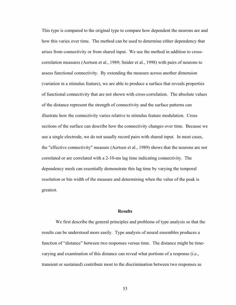
This type is compared to the original type to compare how dependent the neurons are and

how this varies over time. The method can be used to determine either dependency that

arises from connectivity or from shared input. We use the method in addition to cross-

correlation measures (Aertsen et al., 1989; Snider et al., 1998) with pairs of neurons to

assess functional connectivity. By extending the measure across another dimension

(variation in a stimulus feature), we are able to produce a surface that reveals properties

of functional connectivity that are not shown with cross-correlation. The absolute values

of the distance represent the strength of connectivity and the surface patterns can

illustrate how the connectivity varies relative to stimulus feature modulation. Cross

sections of the surface can describe how the connectivity changes over time. Because we

use a single electrode, we do not usually record pairs with shared input. In most cases,

the "effective connectivity" measure (Aertsen et al., 1989) shows that the neurons are not

correlated or are correlated with a 2-10-ms lag time indicating connectivity. The

dependency mesh can essentially demonstrate this lag time by varying the temporal

resolution or bin width of the measure and determining when the value of the peak is

greatest.

Results We first describe the general principles and problems of type analysis so that the

results can be understood more easily. Type analysis of neural ensembles produces a

function of “distance” between two responses versus time. The distance might be time-

varying and examination of this distance can reveal what portions of a response (i.e.,

transient or sustained) contribute most to the discrimination between two responses as

53

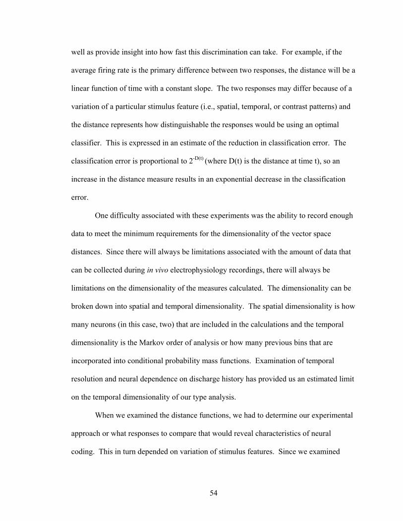
well as provide insight into how fast this discrimination can take. For example, if the

average firing rate is the primary difference between two responses, the distance will be a

linear function of time with a constant slope. The two responses may differ because of a

variation of a particular stimulus feature (i.e., spatial, temporal, or contrast patterns) and

the distance represents how distinguishable the responses would be using an optimal

classifier. This is expressed in an estimate of the reduction in classification error. The

classification error is proportional to 2-D(t) (where D(t) is the distance at time t), so an

increase in the distance measure results in an exponential decrease in the classification

error.

One difficulty associated with these experiments was the ability to record enough

data to meet the minimum requirements for the dimensionality of the vector space

distances. Since there will always be limitations associated with the amount of data that

can be collected during in vivo electrophysiology recordings, there will always be

limitations on the dimensionality of the measures calculated. The dimensionality can be

broken down into spatial and temporal dimensionality. The spatial dimensionality is how

many neurons (in this case, two) that are included in the calculations and the temporal

dimensionality is the Markov order of analysis or how many previous bins that are

incorporated into conditional probability mass functions. Examination of temporal

resolution and neural dependence on discharge history has provided us an estimated limit

on the temporal dimensionality of our type analysis.

When we examined the distance functions, we had to determine our experimental

approach or what responses to compare that would reveal characteristics of neural

coding. This in turn depended on variation of stimulus features. Since we examined

54

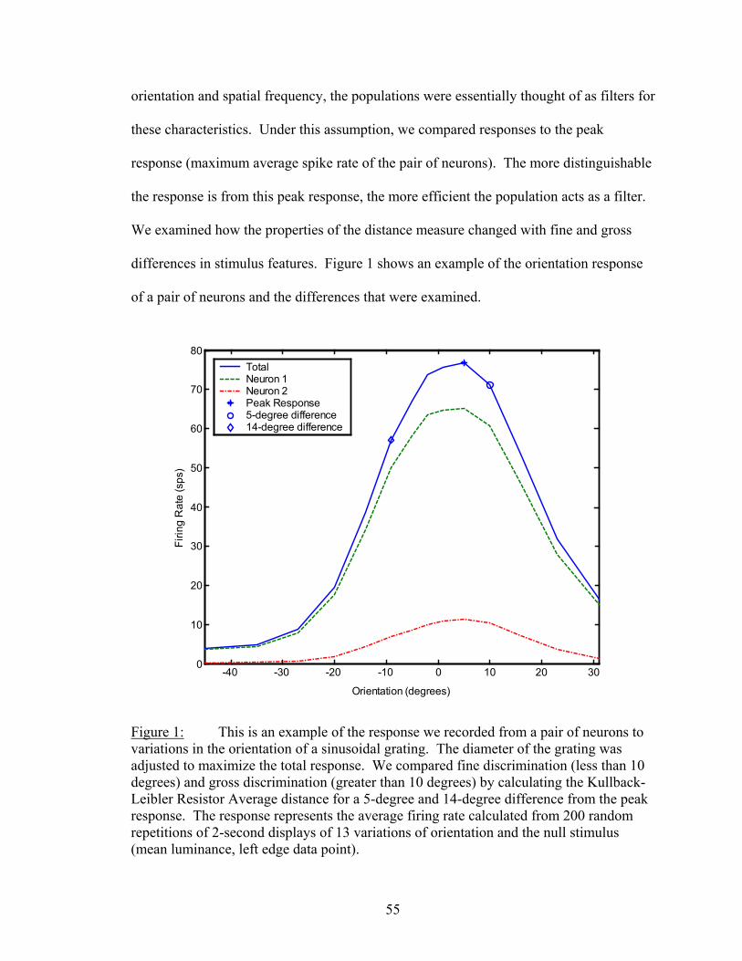
orientation and spatial frequency, the populations were essentially thought of as filters for

these characteristics. Under this assumption, we compared responses to the peak

response (maximum average spike rate of the pair of neurons). The more distinguishable

the response is from this peak response, the more efficient the population acts as a filter.

We examined how the properties of the distance measure changed with fine and gross

differences in stimulus features. Figure 1 shows an example of the orientation response

of a pair of neurons and the differences that were examined.

-40 -30 -20 -10 0 10 20 300

10

20

30

40

50

60

70

80

Firin

g R

ate

(sps

)

Orientation (degrees)

TotalNeuron 1Neuron 2Peak Response5-degree difference14-degree difference

Figure 1: This is an example of the response we recorded from a pair of neurons to variations in the orientation of a sinusoidal grating. The diameter of the grating was adjusted to maximize the total response. We compared fine discrimination (less than 10 degrees) and gross discrimination (greater than 10 degrees) by calculating the Kullback-Leibler Resistor Average distance for a 5-degree and 14-degree difference from the peak response. The response represents the average firing rate calculated from 200 random repetitions of 2-second displays of 13 variations of orientation and the null stimulus (mean luminance, left edge data point).

55

Latency

We first examined the contribution of latency differences in distinguishing

responses. Gawne et al. (1996b) showed that the delay between the start of the stimulus

and the onset of response was strongly modulated by contrast and there was no apparent

modulation with orientation. Peristimulus time histograms (PSTH) in the populations

tested with type analysis showed that latency continuously decreased for increasing

contrast and varied for orientation differences, but did not vary for spatial frequency

changes. The modulation was clearly organized for contrast, but there was no apparent

correlation between latency and orientation. We observed that while the latency varied as

much as 9-10 ms with orientation, there was no relationship between latency and a

particular orientation in the tuning curve.

Figure 2 demonstrates how precise measurement of latency differences can

improve the discrimination between responses to two different orientations. The top two

plots are the PSTHs for the first 100 ms of each neuron in the ensemble pair. The bottom

plot is one half of the Resistor Average distance accumulated over the first 100 ms. The

initial step seen in the distance function calculated between the two responses starting

from stimulus onset is caused by a precise 9 ms difference in latency between the two

responses, which is apparent from observation of the PSTHs. The 0.5 bit of distance can

reduce the error in classification by nearly 30%. To verify that this step was caused by

the latency difference, the responses were tested after shifting one response by 9 ms to

match the onset of the other response. Since the two responses had similar firing rates,

the distance for the first 100 ms between the two responses is nearly zero when

compensating for the latency difference. This particular case demonstrates one of the

56

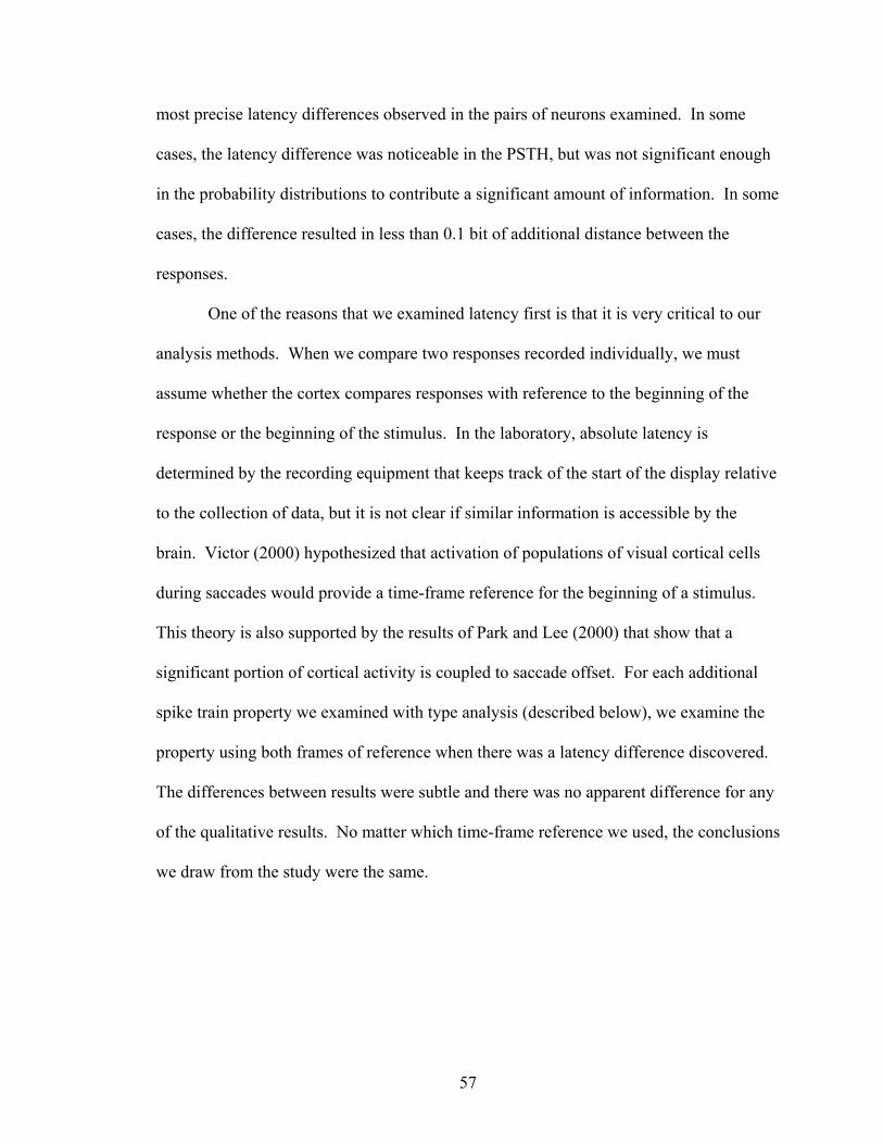
most precise latency differences observed in the pairs of neurons examined. In some

cases, the latency difference was noticeable in the PSTH, but was not significant enough

in the probability distributions to contribute a significant amount of information. In some

cases, the difference resulted in less than 0.1 bit of additional distance between the

responses.

One of the reasons that we examined latency first is that it is very critical to our

analysis methods. When we compare two responses recorded individually, we must

assume whether the cortex compares responses with reference to the beginning of the

response or the beginning of the stimulus. In the laboratory, absolute latency is

determined by the recording equipment that keeps track of the start of the display relative

to the collection of data, but it is not clear if similar information is accessible by the

brain. Victor (2000) hypothesized that activation of populations of visual cortical cells

during saccades would provide a time-frame reference for the beginning of a stimulus.

This theory is also supported by the results of Park and Lee (2000) that show that a

significant portion of cortical activity is coupled to saccade offset. For each additional

spike train property we examined with type analysis (described below), we examine the

property using both frames of reference when there was a latency difference discovered.

The differences between results were subtle and there was no apparent difference for any

of the qualitative results. No matter which time-frame reference we used, the conclusions

we draw from the study were the same.

57

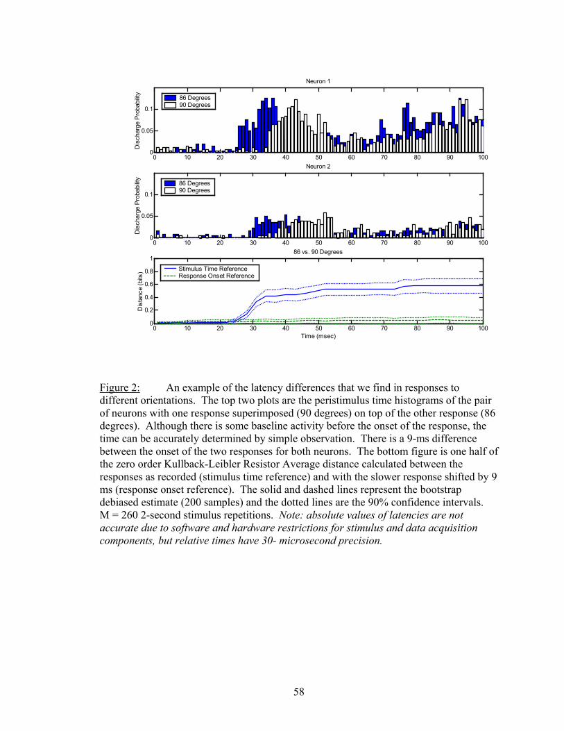
0 10 20 30 40 50 60 70 80 90 1000

0.05

0.1

Neuron 2

Dis

char

ge P

roba

bility 86 Degrees

90 Degrees

0 10 20 30 40 50 60 70 80 90 1000

0.05

0.1

Dis

char

ge P

roba

bilit

y

Neuron 1

86 Degrees90 Degrees

0 10 20 30 40 50 60 70 80 90 1000

0.2

0.4

0.6

0.8

1

Time (msec)

Dis

tanc

e (b

its)

86 vs. 90 Degrees

Stimulus Time ReferenceResponse Onset Reference

Figure 2: An example of the latency differences that we find in responses to different orientations. The top two plots are the peristimulus time histograms of the pair of neurons with one response superimposed (90 degrees) on top of the other response (86 degrees). Although there is some baseline activity before the onset of the response, the time can be accurately determined by simple observation. There is a 9-ms difference between the onset of the two responses for both neurons. The bottom figure is one half of the zero order Kullback-Leibler Resistor Average distance calculated between the responses as recorded (stimulus time reference) and with the slower response shifted by 9 ms (response onset reference). The solid and dashed lines represent the bootstrap debiased estimate (200 samples) and the dotted lines are the 90% confidence intervals. M = 260 2-second stimulus repetitions. Note: absolute values of latencies are not accurate due to software and hardware restrictions for stimulus and data acquisition components, but relative times have 30- microsecond precision.

58

Temporal Resolution

We next examined the temporal resolution used to bin the responses. Although

recordings were done with 30-microsecond precision, the responses were represented as a

“letter” determined by which neurons had a spike occur within a longer time window.

Temporal resolution was varied from 1 ms to 8 ms for analysis of responses for

discrimination of fine and gross changes of orientation and spatial frequency. Ten pairs

of neurons were examined for orientation differences of less than 10 degrees and greater

than 10 degrees from the peak response, and 10 pairs of neurons for spatial frequency

differences of less than 0.1 c/deg or greater than 0.1 c/deg. The number of stimulus

repetitions collected for each pair of neurons ranged from 30 to 300 with a mean of 195.

In our initial observations of distance rate versus bin width, we found an inversely

proportional relationship with temporal resolution for 8 pairs of neurons. Johnson et al.

(2001) predict that the bin width should be essentially independent of the distance rate or

accumulated distance when discharge probabilities are relatively small. These

predictions are made for a single neuron, zero Markov order scenario where the response

difference is a difference in average firing rates. This of course does not mean that a

distance measure of an actual neural response cannot vary as some function of temporal

resolution. However, a closer look at the 8 pairs of cells with the inversely proportional

relationship revealed that these pairs had either a relatively weak pooled response (<30

sps) or a small number of stimulus repetitions (<100) suggesting that the amount of data

available for the distance measure was insufficient. Smaller bin size results in a lower

probability of nonzero letters occurring in each bin. Across 2000 1-ms bins, even with

100 repetitions there will be instances when a bin is empty. The limited amount of data

59

leads to additional bias resulting in a larger estimate and a wider confidence interval. The

bootstrap method permits an estimation of the bias, but a limited amount of data will still

prevent the method from making accurate estimates. In these cases, the imprecision of

the estimate was indicated by large confidence intervals. As the data approaches larger

firing rates and larger differences in firing rate or larger bin widths and larger numbers of

samples, the distance rate does essentially become independent from the bin width.

There is still another irregularity seen in our results. In the case of stronger responses, we

consistently see a rise in the distance rate versus bin width over the 2-5-ms range. In

some cases, there is still a slight rise from a bin width of 2 ms to 1 ms and wider 90%

confidence intervals at 1ms, but the rise in the 2-5-ms range is still evident.

We examined this relationship for 7 pairs of neurons for orientation

discrimination and 5 pairs for spatial frequency discrimination. These recordings had a

pooled response of 36-109 sps with 120-300 stimulus repetitions (an average of 235).

Our definition of fine discrimination of orientation (<10 degrees) resulted in an average

rate difference of 7.6 sps (range 4-11) or a 10.5% difference (range 6.1-16.5), and the

definition of gross discrimination of orientation (>10 degrees) resulted in an average rate

difference of 30.6 sps (range 21-49) or a 43.0% difference (range 33.3-58.3). For fine

discrimination of spatial frequency (<0.1 c/deg) the average difference was 9.2 sps (range

4-13) or an 11.8% difference (range 5.8-14.6), and for gross discrimination (>0.1 c/deg)

the average difference was 24.6 sps or a 31.7% difference (range 28.7-34.1).

There are two possibilities for the reason there is an advantage in discriminating

neural responses (an increase in distance rate) in this range of temporal resolutions (2-5

ms). First, independent interspike interval (ISI) statistics over the short term (i.e.,

60

bursting) carry information about the stimulus feature being discriminated (e.g., Debusk

et al., 1997) and this information is extracted by filtering the response to emphasize this

time frame. Second, dependent ISI statistics (i.e., connectivity) between the pair of

neurons carries stimulus related information that provides the best discrimination within

this temporal window. To test for both of these possibilities, we first measure the

distance rates versus bin width of the original responses and then measure the function

after shuffling the stimulus repetitions for each neuron to remove spike train

dependencies.

Figure 3 shows an example of the distance rate function for fine (3A) and gross

(3B) discrimination of spatial frequency, along with fine (3C) and gross (3D)

discrimination of orientation. Although in some cases the advantage is subtle, it is clear

there is a peak from 2-4 ms for the original responses for all discriminations. After the

responses were shuffled (dashed lines), the peak remains, demonstrating that independent

ISI properties of the responses provide significant advantages for both orientation and

spatial frequency discrimination. Another subtle characteristic that was seen in all 12

pairs of neurons is that after shuffling the responses, the peak tended to shift to a higher

temporal resolution and the bandwidth of this peak was narrower. The average peak for

the 12 pairs of neurons for fine discrimination was at 3.5 ms with a width of 4.3 ms

(34.4% increase at peak), and after shuffling, the peak was at 2.3 ms with a width of 3.5

ms (67.9% increase at peak). The average peak for gross discrimination was at 3.5 ms

with a width of 6.5 ms (15.8% increase at peak), and after shuffling, the peak was at 2.7

ms with a width of 4.8 ms (29.5% increase at peak). For both small and large stimulus

differences, the results suggest an optimal bin width in the range of 2-5 ms.

61

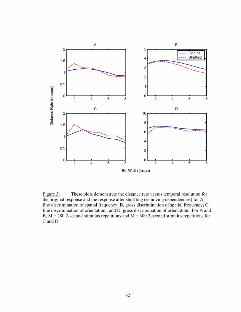
2 4 6 80

0.5

1

1.5

2D

ista

nce

Rat

e (b

its/s

ec)

A

2 4 6 80

1

2

3

4

5B

OriginalShuffled

2 4 6 80

0.5

1

1.5

2C

2 4 6 80

2

4

6

8

10

Bin Width (msec)

D

OriginalShuffled

Figure 3: These plots demonstrate the distance rate versus temporal resolution for the original response and the response after shuffling (removing dependencies) for A, fine discrimination of spatial frequency; B, gross discrimination of spatial frequency; C, fine discrimination of orientation.; and D, gross discrimination of orientation. For A and B, M = 280 2-second stimulus repetitions and M = 300 2-second stimulus repetitions for C and D.

62

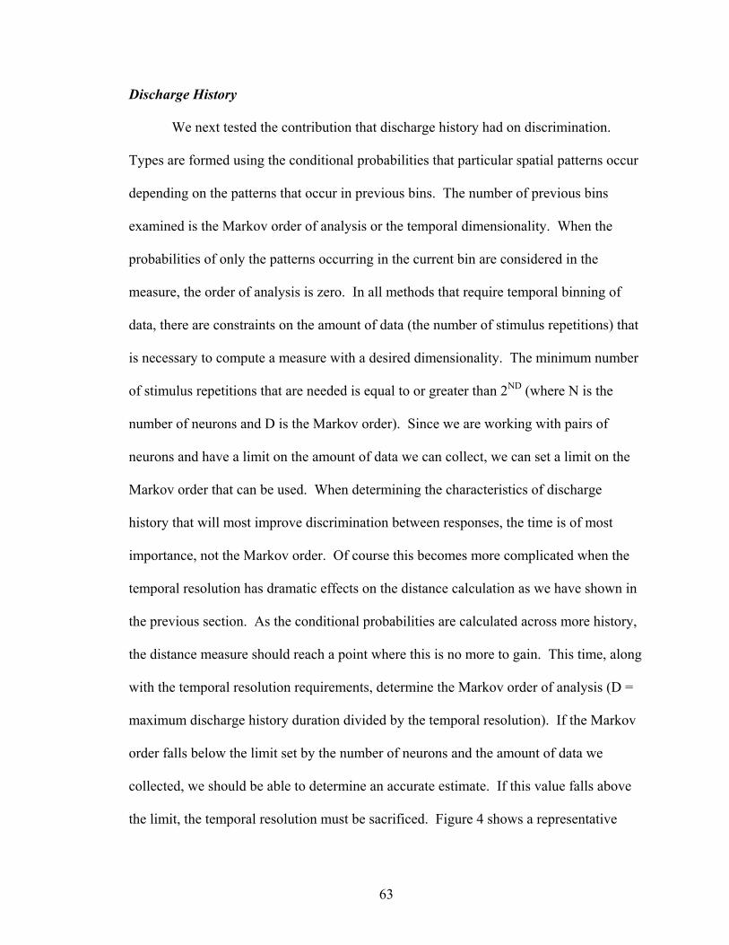
Discharge History

We next tested the contribution that discharge history had on discrimination.

Types are formed using the conditional probabilities that particular spatial patterns occur

depending on the patterns that occur in previous bins. The number of previous bins

examined is the Markov order of analysis or the temporal dimensionality. When the

probabilities of only the patterns occurring in the current bin are considered in the

measure, the order of analysis is zero. In all methods that require temporal binning of

data, there are constraints on the amount of data (the number of stimulus repetitions) that

is necessary to compute a measure with a desired dimensionality. The minimum number

of stimulus repetitions that are needed is equal to or greater than 2ND (where N is the

number of neurons and D is the Markov order). Since we are working with pairs of

neurons and have a limit on the amount of data we can collect, we can set a limit on the

Markov order that can be used. When determining the characteristics of discharge

history that will most improve discrimination between responses, the time is of most

importance, not the Markov order. Of course this becomes more complicated when the

temporal resolution has dramatic effects on the distance calculation as we have shown in

the previous section. As the conditional probabilities are calculated across more history,

the distance measure should reach a point where this is no more to gain. This time, along

with the temporal resolution requirements, determine the Markov order of analysis (D =

maximum discharge history duration divided by the temporal resolution). If the Markov

order falls below the limit set by the number of neurons and the amount of data we

collected, we should be able to determine an accurate estimate. If this value falls above

the limit, the temporal resolution must be sacrificed. Figure 4 shows a representative

63

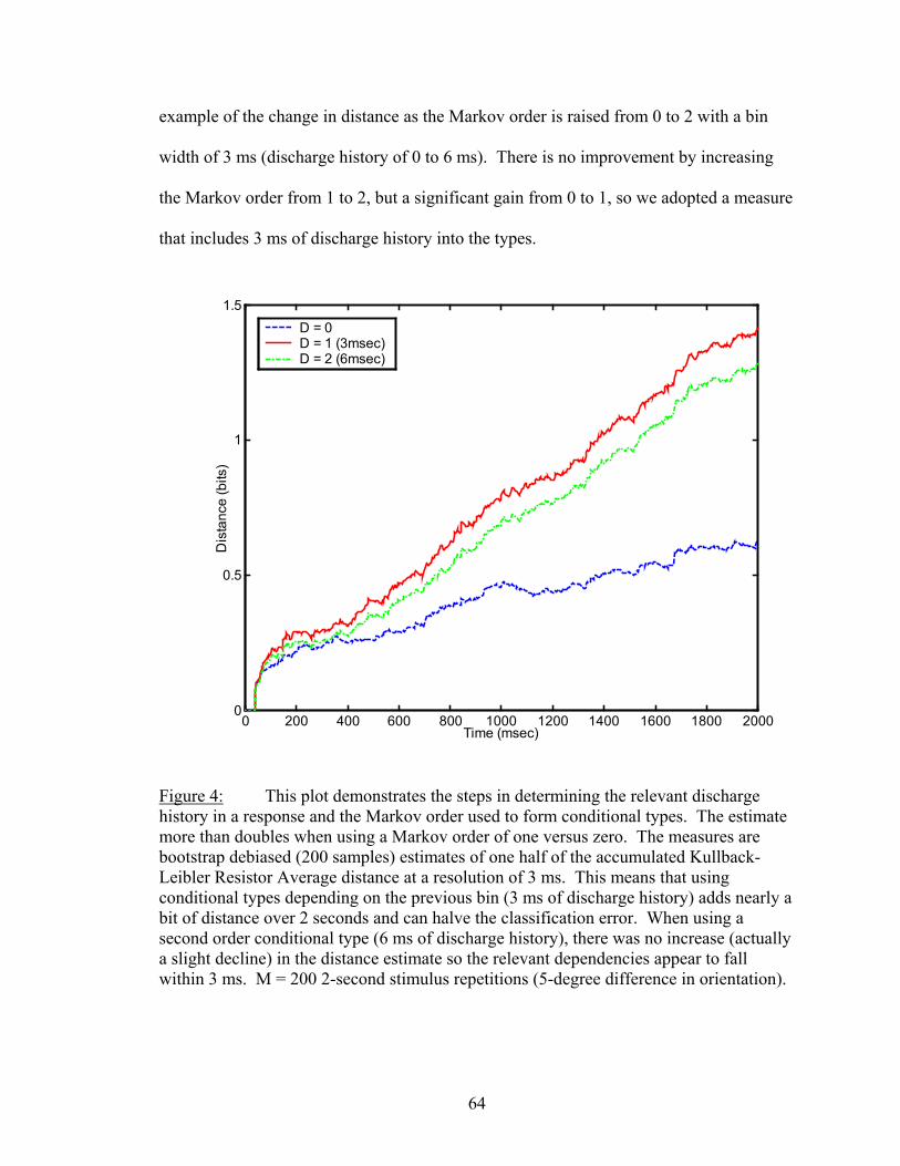
example of the change in distance as the Markov order is raised from 0 to 2 with a bin

width of 3 ms (discharge history of 0 to 6 ms). There is no improvement by increasing

the Markov order from 1 to 2, but a significant gain from 0 to 1, so we adopted a measure

that includes 3 ms of discharge history into the types.

0 200 400 600 800 1000 1200 1400 1600 1800 20000

0.5

1

1.5

Dis

tanc

e (b

its)

Time (msec)

D = 0D = 1 (3msec)D = 2 (6msec)

Figure 4: This plot demonstrates the steps in determining the relevant discharge history in a response and the Markov order used to form conditional types. The estimate more than doubles when using a Markov order of one versus zero. The measures are bootstrap debiased (200 samples) estimates of one half of the accumulated Kullback-Leibler Resistor Average distance at a resolution of 3 ms. This means that using conditional types depending on the previous bin (3 ms of discharge history) adds nearly a bit of distance over 2 seconds and can halve the classification error. When using a second order conditional type (6 ms of discharge history), there was no increase (actually a slight decline) in the distance estimate so the relevant dependencies appear to fall within 3 ms. M = 200 2-second stimulus repetitions (5-degree difference in orientation).

64

We also wanted to examine how discharge history contributed to discrimination

regardless of the temporal resolution. Because the temporal resolution had such a

significant effect on the distance measure, it distorts the effects of discharge history when

looking at the average distance rate alone. To separate out this distortion, we calculated

the increase in distance from a zero order calculation to a first order calculation at several

bin widths.

Responses from 11 of the 12 pairs of neurons (7 orientation, 4 spatial frequency)

were tested for bin widths from 1 ms to 6 ms to determine the impact of discharge

history. As with temporal resolution, both independent and dependent spike train

characteristics can lead to advantages in discrimination as a result of the discharge history

information. For example, burst length modulation will lead to significant changes in the

probabilities of spikes occurring in the discharge history of the individual neurons. At

the same time, connectivity modulation will be revealed in discharge histories that

include enough time to allow for synaptic delays. To separate the contributions of

independent and dependent properties, we again compared the original results with the

result after shuffling the stimulus repetitions for each neuron.

Figure 5 shows an example of the results for fine (A and C) and gross (B and D)

discrimination of orientation for a pair of moderately connected neurons (we find a

noticeable peak at 2-10 ms in the correlogram or a dependency between the neurons of

greater than 0.1 bits/s—see Functional Connectivity for a detailed explanation). For fine

orientation discrimination (Figure 5A), the optimal amount of discharge history is 2 ms

(providing 110% increase in distance). After shuffling the responses, we see that the

independent properties of discharge history (Figure 5A, black bars) are not as strongly

65

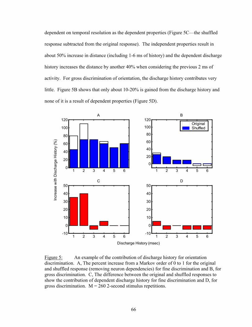
dependent on temporal resolution as the dependent properties (Figure 5C—the shuffled

response subtracted from the original response). The independent properties result in

about 50% increase in distance (including 1-6 ms of history) and the dependent discharge

history increases the distance by another 40% when considering the previous 2 ms of

activity. For gross discrimination of orientation, the discharge history contributes very

little. Figure 5B shows that only about 10-20% is gained from the discharge history and

none of it is a result of dependent properties (Figure 5D).

1 2 3 4 5 60

20

40

60

80

100

120

Incr

ease

with

Dis

char

ge H

isto

ry (%

)

A

1 2 3 4 5 6-10

0

10

20

30

40

50

Discharge History (msec)

C

1 2 3 4 5 6

0

20

40

60

80

100

120B

OriginalShuffled

1 2 3 4 5 6-10

0

10

20

30

40

50D

Figure 5: An example of the contribution of discharge history for orientation discrimination. A, The percent increase from a Markov order of 0 to 1 for the original and shuffled response (removing neuron dependencies) for fine discrimination and B, for gross discrimination. C, The difference between the original and shuffled responses to show the contribution of dependent discharge history for fine discrimination and D, for gross discrimination. M = 260 2-second stimulus repetitions.

66

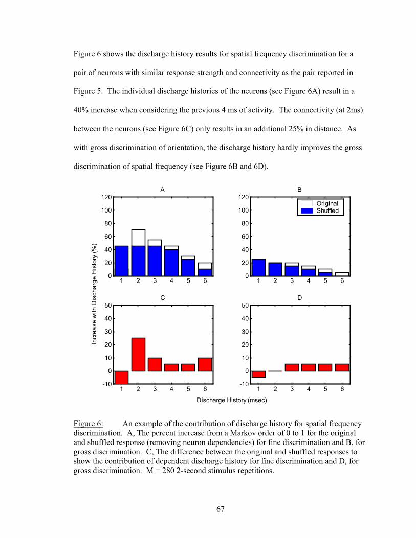
Figure 6 shows the discharge history results for spatial frequency discrimination for a

pair of neurons with similar response strength and connectivity as the pair reported in

Figure 5. The individual discharge histories of the neurons (see Figure 6A) result in a

40% increase when considering the previous 4 ms of activity. The connectivity (at 2ms)

between the neurons (see Figure 6C) only results in an additional 25% in distance. As

with gross discrimination of orientation, the discharge history hardly improves the gross

discrimination of spatial frequency (see Figure 6B and 6D).

1 2 3 4 5 60

20

40

60

80

100

120A

1 2 3 4 5 6-10

0

10

20

30

40

50

Incr

ease

with

Dis

char

ge H

isto

ry (%

)

Discharge History (msec)

C

1 2 3 4 5 60

20

40

60

80

100

120B

OriginalShuffled

1 2 3 4 5 6-10

0

10

20

30

40

50D

Figure 6: An example of the contribution of discharge history for spatial frequency discrimination. A, The percent increase from a Markov order of 0 to 1 for the original and shuffled response (removing neuron dependencies) for fine discrimination and B, for gross discrimination. C, The difference between the original and shuffled responses to show the contribution of dependent discharge history for fine discrimination and D, for gross discrimination. M = 280 2-second stimulus repetitions.

67

The average overall increase in distance (for 7 pairs) when incorporating 2 ms of

discharge history for fine discrimination of orientation was 110% (range 55-250). After

shuffling the stimulus repetitions for each neuron, the average increase was 60% (range

45-90). Discharge history provided on average only 15% (range 0-35) for gross

discrimination of orientation and the average did not change after removing dependencies

between the neurons. For spatial frequency discrimination, the contribution was less

significant for fine differences, yielding an average increase (for 4 pairs) of 70% (range

40-120) including dependencies and 50% (range 40-75) without dependencies. As with

orientation, there was very little to gain for discrimination of gross changes in spatial

frequency with an average increase in distance of 20% (range 5-25) before and after

shuffling the responses. Overall, the results suggest that the dependent properties of

discharge history between the neurons can provide an average of 50% for fine

discriminations of orientation and 20% for fine discriminations of spatial frequency, and

provide no significant improvement in gross discriminations of both orientation and

spatial frequency. In the next section, we derive similar results using a different approach

to show how dependent ISI properties enhance discriminations of features. We will also

evaluate the confidence of these results with respect to the amount of data we use in the

distance calculations.

Synergy, independence, and redundancy

We next demonstrate how incorporation of discharge history leads to additional

information beyond what would be derived from the individual neurons. Efforts thus far

have demonstrated that visual cortical pairs are independent (Gawne et al., 1996a; Victor,

68

2000; Reich et al., 2001c). We examined our data to see whether the responses of

neurons were independent or if under some conditions, examining them as a population

leads to additional information.

The Kullback-Leibler Resistor Average distances were calculated for the same 11

pairs of neurons mentioned above and for each individual neuron in the pairs. The

individual neurons’ types are formed from a 2-letter alphabet (discharge or no discharge)

whereas the ensemble type is formed from a 4-letter alphabet (both discharged, only

neuron 1 discharged, only neuron 2 discharged, or neither discharged). We also

calculated the first order distances using the optimal parameters for bin width and

discharge history that were determined with the ensemble measures. If the ensemble

measures were greater than the sum of the individual neurons’ measures, then the neurons

were cooperating and producing additional information (synergy). If the ensemble

measure was less than the sum, the neurons contained redundant information about the

stimulus differences. If both the ensemble measure and sum of the individual measures

are equal, the neurons are acting independently. If the first order measures for the

individual neurons show either no gain (from the zero order measure) or a relatively

small gain compared to the gain for the ensemble first order measure, then the gain seen

in the ensemble measure is a result of correlation between the neurons rather than any

auto-correlation found in the individual neurons.

The results we found were similar to the results found when examining discharge

history, implying that a significant portion of the additional information gained from

discharge history is a result of the correlated activity between the neurons. This also

means that a significant portion of the synergy is a result of incorporating the discharge

69

history into the distance measure. We also find that the cooperation is related to the

strength of connectivity between the neurons. The average amount of synergy produced

across all 7 pairs of neurons for fine discrimination of orientation was 50%, with a range

covering 15-120%. Regardless of the connectivity, the neurons for the most part work

independently for gross discrimination of orientation (synergy of only 5% over the range

of 0-15%). The difference between fine and gross discrimination of orientation for

strongly connected neurons was thus nearly 10-fold. As pairs showed less connectivity,

this difference diminished to insignificance for the weakest pair of neurons.

For spatial frequency discrimination, synergy appeared to be lower. The average

amount of distance added as a result of cooperation was 25% for fine discrimination over

the range of 15-40%. The results for gross discrimination of spatial frequency were

nearly the same as gross discrimination of orientation with an average of 8% over the

range of 5-10%. There was at most an 8-fold increase in the percentage gained for fine

discrimination versus gross discrimination for strongly connected neurons and again, the

difference was much smaller for moderately connected neurons.

The example shown in Figure 7A and 7B shows the responses of a pair of neurons

(same pair as in Figure 5) from a 4-degree difference in orientation (4 sps difference with

60 sps peak) and a 16-degree difference (22 sps difference). The ensemble distance is

more than 45% greater than the sum of the individual measures (see Figure 7A). The

larger orientation difference results show that the neurons are acting more independently

(see Figure 7B). The increase is only about 10% and the independent measure falls well

within the lower bound on the 90% confidence interval. This example is for a pair of

70

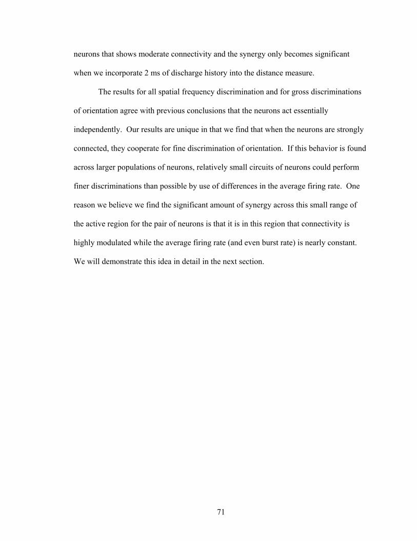
neurons that shows moderate connectivity and the synergy only becomes significant

when we incorporate 2 ms of discharge history into the distance measure.

The results for all spatial frequency discrimination and for gross discriminations

of orientation agree with previous conclusions that the neurons act essentially

independently. Our results are unique in that we find that when the neurons are strongly

connected, they cooperate for fine discrimination of orientation. If this behavior is found

across larger populations of neurons, relatively small circuits of neurons could perform

finer discriminations than possible by use of differences in the average firing rate. One

reason we believe we find the significant amount of synergy across this small range of

the active region for the pair of neurons is that it is in this region that connectivity is

highly modulated while the average firing rate (and even burst rate) is nearly constant.

We will demonstrate this idea in detail in the next section.

71

0 500 1000 1500 20000

0.5

1

1.5

2

2.5

3A

Ensemble DistanceNeuron 1Neuron 2Neuron 1 + 2

0 500 1000 1500 20000

2

4

6

8

Time (msec)

Dis

tanc

e (b

its)

B

Figure 7: An example of the synergy found in a moderately connected pair of neurons during orientation discrimination (same pair of neurons as in Figure 5). A, One half of the accumulated Kullback-Leibler Resistor Average distances calculated from the 4-letter ensemble type (solid), calculated from the 2-letter types for each neuron (dash-dot), and the sum of the two independent neuron types (dash-dash). The accumulated distance is between the peak response and the response to an orientation 4 degrees from the peak orientation, which had a difference in total firing rate less than 10%. The synergy results in a 45% increase, but it should be noted that the 90% confidence interval (dotted) is relatively large. B, The same four measures as in plot A except for the accumulated distance between the peak response and to an orientation 16 degrees from the peak orientation. The synergy results in a 10% increase and the lower bound on the confidence interval falls well below the independent distance. All calculations were done with bin widths of 2 ms and a Markov order of one. Estimates and confidence intervals were calculated with the bootstrap method (200 samples). M = 260 2-second stimulus repetitions.

72

Confidence in distance estimations

The imprecision in the first order ensemble distance (incorporating 2 ms of

history) is still evident even with our large sample sizes. This is seen in Figure 7A where

the independent distance falls within the lower bound of the 90% confidence interval.

This raises the question as to the accuracy of our distance calculations (both relative and

absolute) for both discharge history and synergy. We performed analysis on all 20 pairs

of neurons to examine how confident we were in our calculations in addition to what the

confidence interval demonstrated. We initially rejected 8 of the 20 possible pairs of

neurons (for orientation and spatial frequency analysis) because the temporal resolution

plots suggested insufficient sampling due to an inversely proportional relationship of

distance rate with bin width. We rejected another pair of neurons for our discharge

history analysis based on significant inconsistencies between the synergy and discharge

history analysis. We also rejected this pair of neurons for synergy analysis after

examining the relationship of our calculations to sample size.

For each pair of neurons, we randomly selected one-half, five-eighths, three-

fourths, and seven-eighths of the available stimulus repetitions and plotted the ensemble

distance rate, the independent distance rate, the two individual neuron distance rates, and

the percent synergy versus the sample size. Figure 8 shows an example of these

calculations for the pair of neurons reported in Figure 7. Figure 8A and Figure 8C show

the distance rates and synergy for fine discrimination of orientation, respectively, and

Figure 8B and Figure 8D for gross discrimination of orientation. Reich et al. (2001a)

examined an information-theoretic-based measure in a similar manner and rejected all

data that resulted in a measure that was in excess of 10% when using a random selection

73

of half the sample versus all of the samples. With our analysis, we could not set such a

criteria without rejecting all of the data, but we do have a sufficient number of samples to

demonstrate that the calculations appear to approach an asymptote versus sample size. At

the same time, the 90% confidence intervals narrow as we select a larger portion of our

sample demonstrating that the precision does continue to increase with the number of

stimulus repetitions.

In general, our sub-sampling analysis showed that with less than 200 stimulus

repetitions, the distance measures and percentage calculations were very unpredictable.

At around 200 repetitions, the distance rates appear to have somewhat of an inversely

proportional relationship with the number of samples and approach asymptotic behavior.

This relationship seems to suggest that fewer samples result in greater discrimination, but

this increase in distance is a result in bias that is not removed with the bootstrap method.

This is clear when observing that the 90% confidence interval grows larger as the sample

size is reduced, and that the lower bound of the interval shows a constant relationship

with sample size. After 250 repetitions, the measures appear to be stable and additional

samples result in less than a 10% difference in the calculations. This behavior is also

dependent on the strength of the response (i.e., the number of spikes) and whether we are

looking at gross versus fine discrimination calculations. In some cases, we found as little

as 120 stimulus repetitions to be sufficient for a pair of neurons with a pooled response of

109 sps. At the same time, we rejected a pair of neurons that only had a response

strength of 31 sps even after 300 stimulus repetitions. A close look at Figure 8A and

Figure 8C versus Figure 8B and Figure 8D reveals that the gross discrimination

74

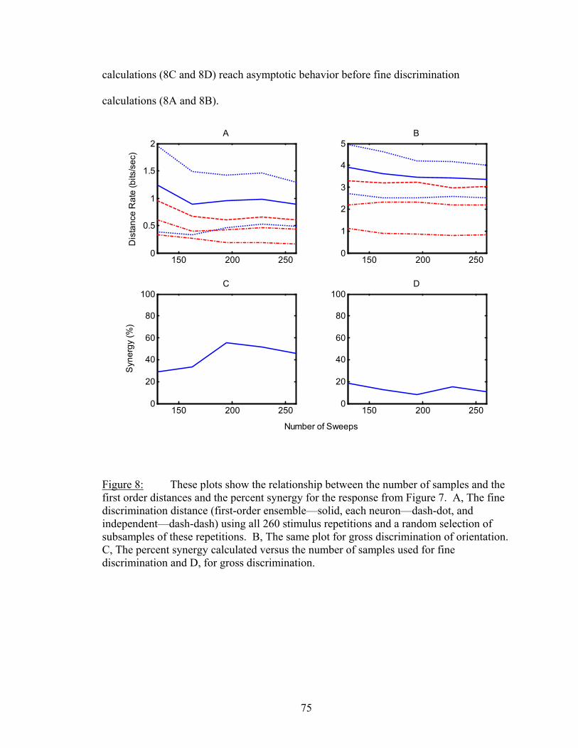
calculations (8C and 8D) reach asymptotic behavior before fine discrimination

calculations (8A and 8B).

150 200 2500

0.5

1

1.5

2D

ista

nce

Rat

e (b

its/s

ec)

A

150 200 2500

20

40

60

80

100

Number of Sweeps

Syn

ergy

(%)

C

150 200 2500

1

2

3

4

5B

150 200 2500

20

40

60

80

100D

Figure 8: These plots show the relationship between the number of samples and the first order distances and the percent synergy for the response from Figure 7. A, The fine discrimination distance (first-order ensemble—solid, each neuron—dash-dot, and independent—dash-dash) using all 260 stimulus repetitions and a random selection of subsamples of these repetitions. B, The same plot for gross discrimination of orientation. C, The percent synergy calculated versus the number of samples used for fine discrimination and D, for gross discrimination.

75

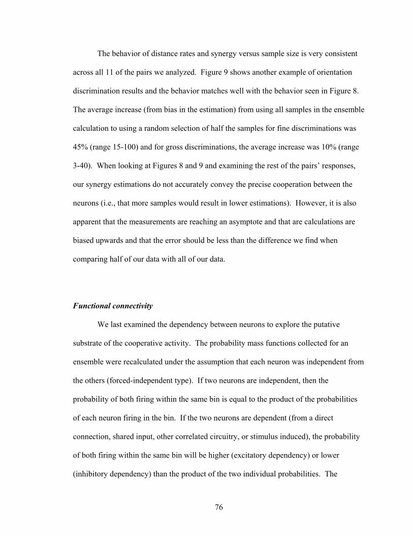
The behavior of distance rates and synergy versus sample size is very consistent

across all 11 of the pairs we analyzed. Figure 9 shows another example of orientation

discrimination results and the behavior matches well with the behavior seen in Figure 8.

The average increase (from bias in the estimation) from using all samples in the ensemble

calculation to using a random selection of half the samples for fine discriminations was

45% (range 15-100) and for gross discriminations, the average increase was 10% (range

3-40). When looking at Figures 8 and 9 and examining the rest of the pairs’ responses,

our synergy estimations do not accurately convey the precise cooperation between the

neurons (i.e., that more samples would result in lower estimations). However, it is also

apparent that the measurements are reaching an asymptote and that are calculations are

biased upwards and that the error should be less than the difference we find when

comparing half of our data with all of our data.

Functional connectivity

We last examined the dependency between neurons to explore the putative

substrate of the cooperative activity. The probability mass functions collected for an

ensemble were recalculated under the assumption that each neuron was independent from

the others (forced-independent type). If two neurons are independent, then the

probability of both firing within the same bin is equal to the product of the probabilities

of each neuron firing in the bin. If the two neurons are dependent (from a direct

connection, shared input, other correlated circuitry, or stimulus induced), the probability

of both firing within the same bin will be higher (excitatory dependency) or lower

(inhibitory dependency) than the product of the two individual probabilities. The

76

measurement can provide insight into the correlation and connectivity between neurons

and how it varies over the time period of a stimulus and varies across variation of

stimulus features. The method was tested on pairs of neurons to examine their

interactions and the results were compared with the normalized "effective connectivity"

measure (Aertsen et al., 1989; Snider et al., 1998).

150 200 2500

0.5

1

1.5

2

2.5

Dis

tanc

e (b

its)

A

150 200 2500

20

40

60

80

100

Number of Sweeps

Syn

ergy

(%)

C

150 200 2500

1

2

3

4B

150 200 2500

20

40

60

80

100D

Figure 9: These plots show the relationship between the number of samples and the first order distances and the percent synergy for the response of another pair of neurons for orientation discrimination. A, The fine discrimination distance (first-order ensemble—solid, each neuron—dash-dot, and independent—dash-dash) using all 280 stimulus repetitions and a random selection of subsamples of these repetitions. B, The same plot for gross discrimination of orientation. C, The percent synergy calculated versus the number of samples used for fine discrimination and D, for gross discrimination.

77

We have tested this method on 22 pairs of neurons while varying orientation (10

pairs), spatial frequency (10 pairs), and contrast (9 pairs). Two pairs of neurons were

tested for all three stimulus parameters, two pairs for contrast and orientation, and one

pair for contrast and spatial frequency. All neurons were classified as complex (Skottun

et al., 1991). The number of stimuli repetitions ranges from 30 to 300 with a mean of

191.

The results were used to produce a surface mesh that displays the dependency

variation between the neurons across the stimulus feature variations and across the

stimulus display time (2 seconds). Since we used a single electrode for recording multi-

unit activity, our results focus on connectivity between neurons rather than common input

synchrony between neurons. Waveforms correlated around a zero lag time will overlap

on a single electrode and it is usually too difficult to distinguish the individual

waveforms. Six out of the 22 pairs of neurons were shown to be strongly connected with

a peak in the cross-correlogram at 2-4 ms and a width of 1-3 ms (10 out of the 29

experiments: 5 for orientation, 1 for spatial frequency, and 4 for contrast). Seven pairs of

neurons (4 for orientation runs, 4 for spatial frequency runs, and 2 contrast runs) showed

some moderate correlation in the cross-correlogram and the last 9 pairs of neurons (1 for

orientation, 5 for spatial frequency, and 3 for contrast) showed no noticeable correlated

activity.

One half of the Kullback-Leibler Resistor Average distance (between the original

type and forced-independent type) was calculated for all pairs using a temporal resolution

of 1-13 ms until the peak of the connectivity mesh was reached. The resolution that

resulted in the largest distances tended to be slightly larger than the peak that was found

78

in the cross-correlogram. In cases where the actual peak was only 1-3 ms wide, but the

correlated activity still extended to greater than 10 ms, we found optimal bin widths to be

as large as 12 ms (although this was rarely the case). The smallest optimal bin width was

2 ms for a pair of neurons that had a 2-ms width peak at 2 ms in the cross-correlogram.

The average optimal bin width of moderately and strongly connected pairs of neurons

was 3.1 ms. The largest distance of the mesh plot divided by the stimulus time was used

to produce an average distance rate value to classify the pair of neurons as strongly,

moderately, or weakly connected. We found that in a few cases the range for strongly

and moderately connected neurons could overlap and determined that the method would

be best suited to be used in conjunction with normalized cross correlation analysis. The

reason for the overlap is that the distance measure is an entropy measure and the absolute

value of the distance rate will be influenced by the strength (firing rate) of the response.

Strongly connected neurons had distance rates from 0.9-4.0 bits/sec and in one case, the

rate was as low as 0.4 bits/sec. Moderately connected neurons had distance rates from

0.2-0.9 bits/sec with one case as high as 1.1 bits/sec and weakly connected neurons had

average rates in the range of 0-0.1 bits/sec. We determined a cutoff of 0.1 bits/sec to

classify a pair of neurons as at least moderately connected. This was determined by

examining the 90% confidence intervals and observing a lower limit below 0 (no

significant dependencies) for responses of weakly connected pairs of neurons and

shuffled responses of moderately and strongly connected pairs of neurons.

The reason we represent the strength of connectivity in terms of average distance

rate is to present a value that is independent of the stimulus duration. A closer look at the

temporal dynamics of the connectivity reveals that it varies in time. Figure 10A shows an

79

example of a surface mesh between a pair of moderately connected neurons for

orientation tuning. Figure 10B shows the optimal orientation and progressively non-

optimal orientations as a cross section of time to illustrate the modulations of

connectivity. The slope of the response indicates differences from the predicted

independent probabilities. Horizontal regions in the function indicate that the neurons are

firing independently from one another. A comparison of the distance plots for the peak

response (288 degrees) and 10 degrees (or 15 degrees) from the peak (278 or 273

degrees) shows that from 25 ms to 40 ms (see inset in Figure 10), the response of the

connectivity is equal with a very steep slope (>8.0 bits/sec). Immediately following the

initial 40 ms, the slope drops to less than 0.5 bits/sec for 278 degrees and less than 0.2

bits/sec for 273 degrees suggesting the correlated activity is reduced by a slightly delayed

inhibition. The peak response of correlated activity (as well as away from the peak) also

shows a decline in slope (although the reduction is much less significant than the

inhibition) and the slower time scale (on the order of seconds) suggests there is

adaptation occurring in the correlated activity. For the most part, the temporal dynamics

and the role of inhibition were similar for spatial frequency tuning of dependency.

80

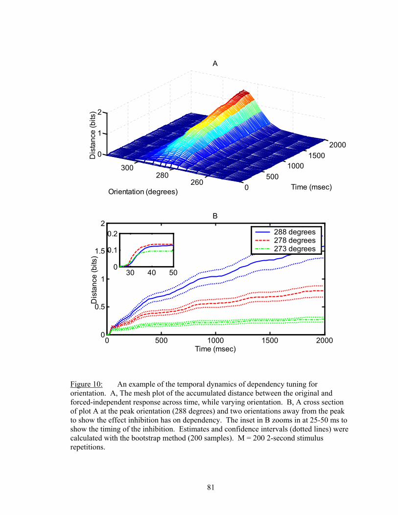
0500

10001500

2000

260280

300

0

1

2

Time (msec)

A

Orientation (degrees)

Dis

tanc

e (b

its)

0 500 1000 1500 20000

0.5

1

1.5

2

Time (msec)

Dis

tanc

e (b

its)

B

288 degrees278 degrees273 degrees

30 40 500

0.1

0.2

Figure 10: An example of the temporal dynamics of dependency tuning for orientation. A, The mesh plot of the accumulated distance between the original and forced-independent response across time, while varying orientation. B, A cross section of plot A at the peak orientation (288 degrees) and two orientations away from the peak to show the effect inhibition has on dependency. The inset in B zooms in at 25-50 ms to show the timing of the inhibition. Estimates and confidence intervals (dotted lines) were calculated with the bootstrap method (200 samples). M = 200 2-second stimulus repetitions.

81

In Figure 10, the contrast was set at 50% for the orientation tuning. We also tested how

contrast would modulate the dependency. We would expect contrast tuning of

dependency to match well with average firing rate tuning because Cattaneo et al.

(1981a,b) demonstrated that all spikes regardless of ISI properties (both bursts and

isolated spikes) followed the same modulation. Figure 11B demonstrates this is clearly

not the case. The dependency modulation (solid line representing the accumulated

distance after 2 seconds) drops off much more rapidly than expected when comparing it

to the firing rate contrast response (dotted lines). The time scale at which the adaptation

in dependency occurs appears to be modulated by the contrast (see Figure 11A).

In order to see the role contrast has in this adaptation, we separate the excitatory

and inhibitory effects seen in the initial portion of the dependency from the slower

adaptation effects. We first converted the dependency responses from accumulated

distances to distance rate functions and filtered the response to remove any modulation.

We then normalized the response by the maximum slope (the initial slope) of that

particular response. This yields a clear picture of how the dependency decomposes from

its original strength at the onset of the response. We can see how contrast affects the

adaptation independently from the strength of the dependency. Figure 12 shows an

example of how this decay or adaptation is effected by contrast. The response at 10% has

a much faster time constant for adaptation than at 60% (or even 20%).

82

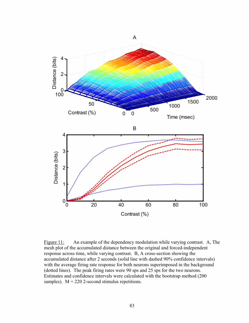
0500

10001500

2000

0

50

1000

2

4

Time (msec)

A

Contrast (%)

Dis

tanc

e (b

its)

0 20 40 60 80 1000

1

2

3

4

Contrast (%)

Dis

tanc

e (b

its)

B

Figure 11: An example of the dependency modulation while varying contrast. A, The mesh plot of the accumulated distance between the original and forced-independent response across time, while varying contrast. B, A cross-section showing the accumulated distance after 2 seconds (solid line with dashed 90% confidence intervals) with the average firing rate response for both neurons superimposed in the background (dotted lines). The peak firing rates were 90 sps and 25 sps for the two neurons. Estimates and confidence intervals were calculated with the bootstrap method (200 samples). M = 220 2-second stimulus repetitions.

83

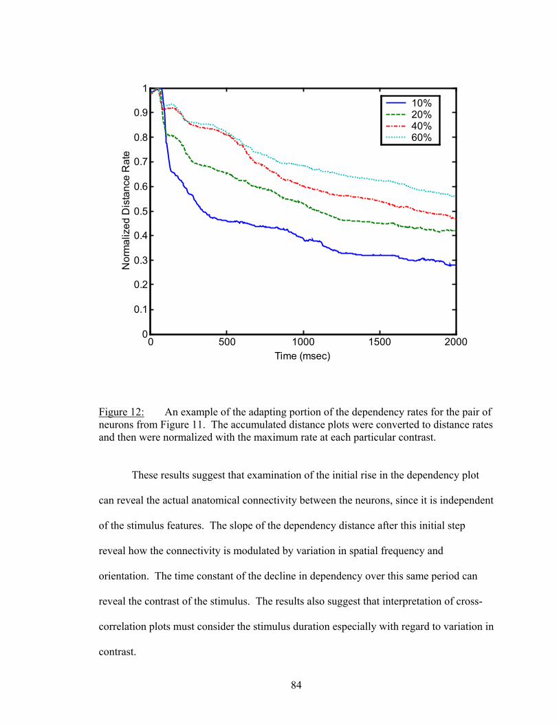
0 500 1000 1500 20000

0.1

0.2

0.3

0.4

0.5

0.6

0.7

0.8

0.9

1

Nor

mal

ized

Dis

tanc

e R

ate

Time (msec)

10%20%40%60%

Figure 12: An example of the adapting portion of the dependency rates for the pair of neurons from Figure 11. The accumulated distance plots were converted to distance rates and then were normalized with the maximum rate at each particular contrast.

These results suggest that examination of the initial rise in the dependency plot

can reveal the actual anatomical connectivity between the neurons, since it is independent

of the stimulus features. The slope of the dependency distance after this initial step

reveal how the connectivity is modulated by variation in spatial frequency and

orientation. The time constant of the decline in dependency over this same period can

reveal the contrast of the stimulus. The results also suggest that interpretation of cross-

correlation plots must consider the stimulus duration especially with regard to variation in

contrast.

84

At first glance, the results appear to suggest that the connectivity modulation for

spatial frequency and orientation are a result of the modulation that occurs in the average

firing rate. Figure 13 is an example of the connectivity tuning we find for a pair of

moderately connected neurons for orientation modulation (A and C) and for spatial

frequency modulation (B and D). In the case of orientation, we find, in all 9 cases of

highly or moderately connected neurons, a very sharp peak of correlation. There were

also sometimes multiple peaks and the highest peak was not always found at the peak of

the average firing rate. Figure 13C shows an example of the dependency tuning with the

rate tuning for the two neurons superimposed in the background. The tuning is much

narrower and allows for much finer discrimination between orientations around the peak.

Figure 13D shows that in the case of spatial frequency, the dependency tuning is slightly

narrower than the rate tuning. Across all cases of connected neurons for spatial

frequency, the tuning was definitely narrower than average rate tuning, but never quite as

drastic as the differences found with orientation tuning.

85

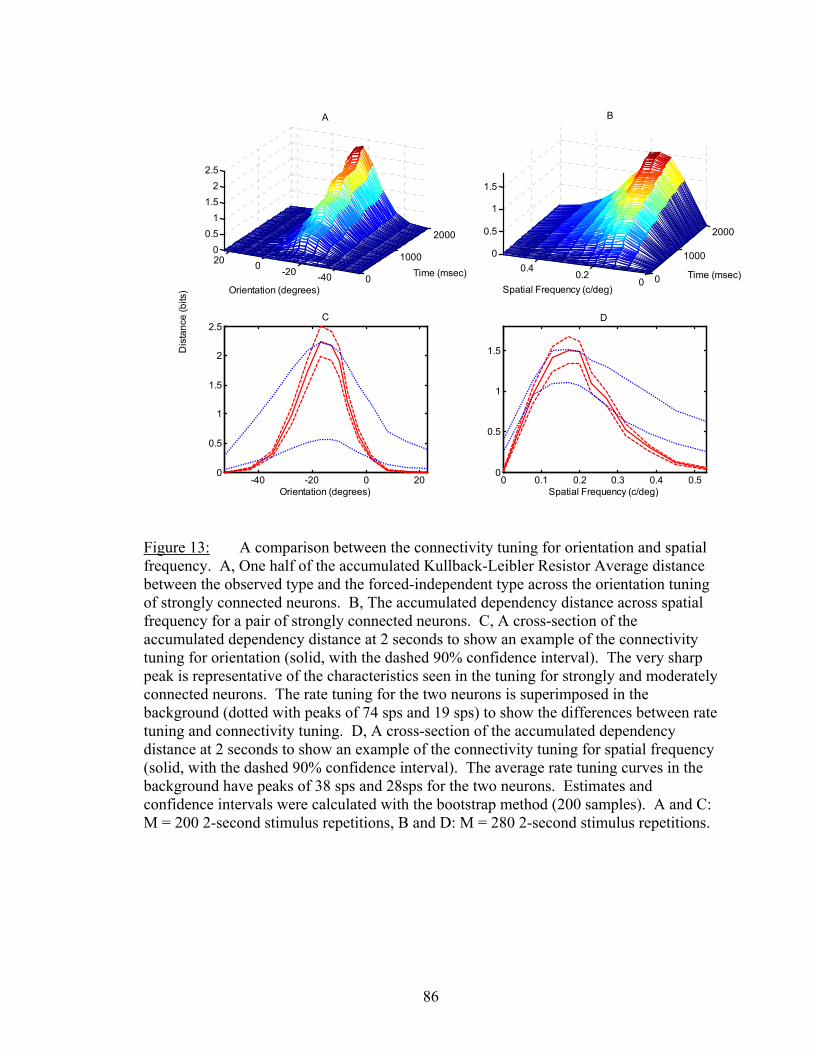
0

1000

2000

-40-200200

0.51

1.52

2.5

Time (msec)

A

Dis

tanc

e (b

its)

-40 -20 0 200

0.5

1

1.5

2

2.5C

Orientation (degrees)

0

1000

2000

00.2

0.40

0.5

1

1.5

Time (msec)

0 0.1 0.2 0.3 0.4 0.50

0.5

1

1.5

Spatial Frequency (c/deg)

D

Orientation (degrees) Spatial Frequency (c/deg)

B

Figure 13: A comparison between the connectivity tuning for orientation and spatial frequency. A, One half of the accumulated Kullback-Leibler Resistor Average distance between the observed type and the forced-independent type across the orientation tuning of strongly connected neurons. B, The accumulated dependency distance across spatial frequency for a pair of strongly connected neurons. C, A cross-section of the accumulated dependency distance at 2 seconds to show an example of the connectivity tuning for orientation (solid, with the dashed 90% confidence interval). The very sharp peak is representative of the characteristics seen in the tuning for strongly and moderately connected neurons. The rate tuning for the two neurons is superimposed in the background (dotted with peaks of 74 sps and 19 sps) to show the differences between rate tuning and connectivity tuning. D, A cross-section of the accumulated dependency distance at 2 seconds to show an example of the connectivity tuning for spatial frequency (solid, with the dashed 90% confidence interval). The average rate tuning curves in the background have peaks of 38 sps and 28sps for the two neurons. Estimates and confidence intervals were calculated with the bootstrap method (200 samples). A and C: M = 200 2-second stimulus repetitions, B and D: M = 280 2-second stimulus repetitions.

86

Discussion

Latency

From an information-theoretic point of view, the importance of the first-spike

timing (latency) was demonstrated by Heller et al. (1995) when they found that latency

accounted for 35% of the total information in V1 and 48% of the total information in IT.

We cannot make any direct comparisons with our results because the percent contribution

of latency to the total distance depends on stimulus duration and the slope of the distance

after the initial step caused by the latency difference, but our results are consistent in

expressing that latency could provide a significant amount of information. The

relationship between latency and contrast has also been established in the primary visual

cortex (Gawne et al., 1996b; Reich et al., 2001b). The role that contrast modulation of

latency might play in neural coding has been postulated as an aid in feature binding

(Gawne et al., 1996b) or that it essentially increases the dynamic range of contrast

encoding by providing finer discriminations than with rate coding (Reich et al., 2001b).

A recent study of pairs of visual cortical neurons showed that latency was

correlated across long distances (>2mm) in the brain and that the variability in the

correlation was less than 10 ms (Fries et al., 2001). This demonstrates the possibility of

the relative latencies between populations of neurons contributing information.

Averaging responses might extract this property as an absolute latency. The variability

found in latency from trial-to-trial is further reduced when considering bursts over all

spikes (Guido and Sherman, 1998).

87

We find latency varies relative to contrast and orientation, but not for spatial

frequency. Latency is also modulated for sound intensity (regardless of location) in

auditory cortex (Heil, 1997) and for motion in area MT (Lisberger and Movshon, 1999).

A dynamic network incorporating delays allows functions such as scaling, rotation, and

translation to occur and is very efficient for invariant applications (Hopfield, 1995;

Schalkoff, 1997). Sensory systems incorporate invariant properties in object recognition,

sound location, and even in odor identification. If the fundamental parameter in visual

processing is spatial frequency (or sound frequency in auditory cortex), then the other

parameters such as orientation, contrast, and temporal frequency (or sound intensity)

would need to be rotated or scaled to provide invariant spatial frequency processing. The

results found thus far are consistent with this idea and spatial frequency would likely be

the invariant parameter for edges, surfaces, and textures that are all incorporated into

object recognition. This does not mean that the properties of orientation, contrast, and

temporal frequency cannot also be encoded within the network.

Artificial networks have been used successfully with time delays for auditory

applications and recently to recognize objects regardless of the velocity and direction of

motion (Wohler and Anlauf, 1999a,b). The research in this area has been limited to

theoretical studies beyond the discovery that spatiotemporal patterns are found to be

modulated by stimuli (Grothe and Klump, 2000). One example of a theoretical study

uses “winner-less competitive” (WLC) networks to produce small dynamic ensembles

within a network to encode olfactory information (Rabinovich et al., 2000).

Current research in axon electrotonic architecture suggest axons themselves are

involved with information processing by inducing delays (Segev and Schneidman, 1999)

88

that would be more efficient than synaptic mechanisms, but Hopfield (1995) points out

that delays might be induced by synaptic, axonal, or cellular mechanisms. The

importance of the temporal dynamics has been stressed in recent reviews (Doetsch, 2000;

Milton and Mackey, 2000; Nadasdy, 2000).

Independent ISI characteristics

The most significant finding in our temporal resolution analysis is the importance

of independent ISI properties in feature discrimination. Since Adrian and Zotterman

(1926) first demonstrated that the average spike rate varied as a function of sensory

stimulation, rate coding has become the most straightforward and popular measurement

in neurophysiological studies. At the same time, it is not necessarily the most

straightforward strategy that the brain might use for encoding (Hopfield, 1995).

Segundo et al. (1963) discovered that interval information was passed between

neurons as a result of temporal integration and synaptic properties. The spike train

contains multiple distributions of activity at various temporal resolutions independently

encoding different aspects of the sensory input (Cattaneo et al., 1981a,b; Debusk et al.,

1997; Victor, 2000). Synaptic properties such as facilitation and depression can take

advantage of these ISI characteristics and could multiplex information on a single neuron

level (Victor, 2000). In any case, the synaptic properties make encoding information in

the form of ISI properties much more straightforward for the brain.

We found a maximization in distance with a temporal resolution of 2-5 ms. We

believe the advantage in using this resolution from 2-5 ms is that it acts like a low pass

filter that emphasizes bursts. Because the difference in the number of bursts in responses

89

to non-optimal stimuli will be greater than the difference in total spike count (Cattaneo et

al., 1981a,b), the discrimination between responses will be easier when the temporal

window selects for the burst count. Reinagel et al. (1999) has shown that information

encoding can be much more efficient when bursts are considered as individual events. A

similar result was found in humoral information transfer, where Prank et al. (2000) used

low pass filtering at frequencies for [Ca2+] bursts to improve transmembrane information

transfer.

Bursts and connectivity

Shadlen and Newsome (1994) have argued that neuronal organization on time

scales less than 10 ms is impractical due to synaptic unreliability. Zador (1998) has

shown that an increase in synaptic reliability (due to changes in transmitter release

probabilities or synaptic redundancy) results in a decrease in information transfer for rate

coding, but an increase in information transfer for temporal coding. Bursting (Snider et

al., 1998) suggests one way to enhance synaptic reliability. In fact, the inefficiency of the

synapse makes it the perfect burst detector (Lisman, 1997). Cattaneo et al. (1981a,b)

demonstrated that over a 60-degree range around the peak of orientation tuning and over

a 0.6-cycles/degree range around the peak of spatial frequency tuning, the average rate of

those spikes not contained in bursts remains essentially constant. This implies that the

rate tuning characteristics are actually a result of burst modulation and all other spikes

might be essentially noise. The efficiency of short spike intervals relative to connectivity

has also been demonstrated from retinal inputs to the thalamus (Usrey et al., 1998)

suggesting the importance of bursts as a signal throughout the visual pathway.

90

Information-theoretic approaches have demonstrated the efficiency of bursts in the LGN

(Reinagal et al., 1999) and visual cortex (Reich et al., 2000). Reich et al. (2000) also

found that the bursts were disproportionately influential to the receptive field properties

of neurons. What might make bursts most suggestive as the fundamental signal are their

reliability from trial-to-trial (Victor et al., 1998).

The low probability of neurotransmitter release along with the high threshold in

the postsynaptic neuron makes it highly unlikely that a single spike will result in a post

synaptic spike. How do two neurons then synchronize within 2ms? They manipulate

both of these characteristics using two different properties of cortical networks. The first

is the aforementioned intrinsic bursting (Gray and McCormick, 1996) that essentially

ensures neurotransmitter release (Lisman, 1997). The second is a result of all the isolated

(or non-burst) spikes found in the lower resolutions of the ISI. Although these spikes

have a low probability of resulting in a postsynaptic spike, there are thousands of

connections so that they will still be passed on across cortical layers, but with a large

amount of variability (Shadlen and Newsome, 1998). These isolated spikes have very

broad tuning (Cattaneo et al., 1981a,b) suggesting they are equally represented across a

large population of neurons. Because these spikes activate a large portion of connections

with a high amount of variability, they result in chaos or an activation of a large amount

of excitatory and inhibitory connections (Shadlen and Newsome, 1998). What this chaos

manipulates is the threshold in the postsynaptic neuron by carefully balancing the

excitation and inhibition. The chaos keeps the postsynaptic potential close to threshold,

but below saturation (Bell et al., 1995).

91

When the postsynaptic neuron is closer to threshold, the neuronal time constant is

reduced and increases the precision of the synchronization between the two neurons. The

chaos can be thought of as background activity and Koch et al. (1996) shows that the

time constant reduces as the background level increases. This is not the background level

typically known as the maintained discharge (present during absence of stimulation), but

rather a subthreshold background level that only becomes evident when stimulation

occurs over the broad range of activation of the isolated spikes.

Functional connectivity and synergy

In order to have synergy, the neural response must contain information in the

form of correlation or synchrony that is not already represented in the individual

responses of the neurons. This can occur when connectivity between neurons modulates

while the individual firing rates remain constant. In the auditory cortex, Frostig et al.

(1983) found that in some cases, there was very little change in presynaptic firing rate

after a connectivity change. This was again demonstrated in the frontal cortex (Vaadia et

al., 1995) where the dynamics of correlation varied between two behaviors while the

firing rate remained the same. We showed that the connectivity between two neurons

continued to modulate while the firing remained nearly constant (near the peak). We also

demonstrated that this could provide as much as a 120% increase in distance between

responses to enhance stimulus discrimination.

We have already discussed how the connectivity is modulated with bursting

behavior and chaos, but have not discussed how the connectivity is modulated relative to

the stimulus properties. By analyzing the temporal dynamics of the connectivity, we

92

were able to gain some insight into how this occurs. The first aspect of functional

connectivity that we observed was that inhibition plays a major role. We found that the

very narrow tuning of connectivity relative to orientation and spatial frequency occurred

only after 15 ms. This time scale is in the same range as the temporal dynamics of

average rate tuning (Volgushev et al., 1995; Ringach et al., 1997), suggesting that the

inhibition we see is a result of feedback interactions. The inhibition may also play a role

in reducing the burst length (Debusk et al., 1997) and explaining why the inhibition for

connectivity/synchrony is more dramatic than for average firing rate.

Contrast has been shown to play a role in normalizing responses in the case of

average firing rate studies (Bonds, 1991; Heeger 1992). Contrast might also modulate

the spatial localization of responses (Sceniak et al., 1999). In our study, we show that

contrast modulates the adaptation (or decay) of connectivity during the stimulus period.

Bonds (1991) showed changes in overall firing rate during the stimulus period, but these

were subtle and in the form of both increases and decreases. The adaptation we find is

much more severe and always shows a decline in the connectivity.

How exactly does contrast modulate this adaptation? This relates back to the

discussion on how chaos modulates the temporal precision of synchronization. Contrast

modulates both bursts and isolated spikes (Cattaneo et al., 1981a,b), and has been shown

to have no effect on burst length modulation (Debusk et al., 1997). The burst rate and

burst length modulation control the initial strength of connectivity between the neurons,

but the isolated spike rate causes the differences in the time constant of this adaptation.

At lower contrasts, the background level (the isolated spikes) will be lower and therefore

the neuron's time constant will be longer (Koch et al., 1996) leading to less precision in

93

the connectivity. Because the precision is reduced, the connectivity essentially ‘falls

apart’ much faster at the lower contrast. So overall, the cortex moves from a short,

distributed, and imprecise pattern of code to a long, localized, and precise pattern as the

contrast is increased.

Orientation discrimination

Psychophysical studies have found orientation discriminations as fine as 10-20' of

arc in untrained human observers (Westheimer, 1981). This is substantially greater than

what would be expected when considering physiological evidence of the most highly

tuned neurons in primates (half-width at half-height of 4 degrees), and the performance is

even better than expected considering the resolution of retinal sampling in humans

(hyperacuities) (Wetsheimer, 1981).

Psychologists have proposed population encoding as a solution to the discrepancy

between the findings. The population schemes are not always so clear in terms of

biological mechanism, with vector summation as the most popular solution (Pouget et al.,

2000). Our results demonstrate how ISI characteristics work together both locally

(bursting) and globally (chaos and synchronization) to encode and transmit information

across populations of neurons. There is information as a result of these fast synaptic

modulations of connectivity that can provide significant contributions to orientation

discriminations. In the present study, we provide clues into some of the temporal

characteristics of this framework, and the next logical step is to examine the spatial

characteristics.

94

CHAPTER III

FUTURE EXPLORATIONS

Introduction

Our recordings of pairs of neurons in the visual cortex of the cat and the analysis

of their spike trains with information theory and cross correlation have shown us that

neurons that show strong connectivity can result in synergy to improve fine

discrimination of orientation. The principal results can be summarized as:

• Discrimination is best at the temporal resolution that matches the peak of bursting

activity in the ISI histogram.

• Incorporating the discharge history that matches the timing of connectivity results in

an advantage and significant cooperation for fine discriminations.

• The modulation of connectivity is a result of excitatory and inhibitory interactions,

and the modulation of connectivity with respect to orientation demonstrates the

contributions of bursts and burst length modulation to synaptic coupling.

The analysis of the temporal dynamics of connectivity has shown us fast modulations of

connectivity that occur within the first 50 ms of the response. The assumptions our

analysis make require a temporal resolution of 2-5 ms and knowledge of the interaction

between neurons within 2-5 ms. The next logical step is to extend this analysis to larger

populations of neurons and examine how the cortex might encode multi-dimensional

visual information under these conditions to form perceptions and perform actions within

100’s of milliseconds. We would also like to take a closer look at data on a trial-by-trial

95

basis to discover what properties of the code are repeated across a population of cortical

cells and therefore more reliable.

The difficulties of obtaining larger population recordings found in our earlier

experiments can be alleviated by using a 10 by 10 or 5 by 5 microelectrode array rather

than a single multi-unit electrode. The 100-microelectrode array should allow us to make

simultaneous recordings of as many as 50 neurons in striate cortex (R.A. Normann, pers.

Comm). The larger number of neurons will allow us to examine the spatiotemporal

patterns that vary according to variation in stimulus features. There is a general

consensus that visual processing must take advantage of populations of neurons

regardless of the theory of the actual encoding characteristics (Pouget et al., 2000; Milton

and Mackey, 2000; Doetsch, 2000; Nadasdy, 2000). The only way to test what

repeatable features occur in neural responses and which features are relevant to the

encoding is to examine larger portions of the cortex simultaneously.

Cortical Function Theory

We believe that cortical encoding needs to be in some ways distributed, but that

cortical architecture (Hubel and Weisel, 1962; DeAngelis et al. 1999) and physiology

(Baddeley et al., 1997; Vinje and Gallant, 2000) suggest that some processing might be

divided among smaller groups of neurons to perform specialized functions. Our theory

from the results in our previous experiments suggest that breaking down our

simultaneous recordings into the proper groups by examining their connectivity will

demonstrate how subgroups cooperate to perform finer encoding of stimulus features.

96

Over the last few years, the interest in temporal coding with bursts, latency, and

spatiotemporal patterns has grown significantly in vision (Bair, 1999) and auditory

(Grothe and Klump, 2000) studies. One of the theories against neuronal organization on

time scale less than 10 ms is the unreliability of the synapse (Shadlen and Newsome,

1994). We believe bursting is a mechanism that allows the cortex to be able to exhibit

the cooperative behavior reliably because of temporal integration (Snider et al., 1998) and

synaptic facilitation (Lisman, 1997). The inefficiency of the synapse results in making

bursting the influential signal for inducing an event in the postsynaptic neuron. We

believe that bursts are the fundamental signal in neural encoding and that the

spatiotemporal connectivity represents the neural code. The results of Cattaneo et al.

(1981a,b) demonstrated that over the tuning range of orientation and spatial frequency,

the average rate of those spikes not contained in bursts remains constant, implying the

rate tuning characteristics are actually a result of the burst modulation.

Our previous results (DeBusk et al., 1997) also demonstrated that stimulus

orientation influences the length of bursts, which in turn has later been shown to result in

more efficient functional connectivity (Snider et al., 1998). We believe this is also

demonstrated in the connectivity tuning demonstrated in the current study (see Functional

Connectivity in Chapter II). The efficiency of bursting relative to connectivity has also

been demonstrated from retinal inputs to the thalamus (Usrey et al., 1998) and in the

LGN with information-theoretic methods (Reinagel et al., 1999) suggesting the

importance of bursts as a signal throughout the visual pathway. What might make

bursting most suggestive as the fundamental signal is its reliability for trial to trial (Victor

et al., 1998; Guido and Sherman, 1998).

97

The other property of neural signals revealed by our analysis of pairs of cells was

the contribution of the isolated (or non-burst) spikes to the strength of synaptic coupling.

By modulating contrast and examining the temporal dynamics of the connectivity, we

discovered that the connectivity decays and that this occurs on a faster time scale for

lower contrasts. We believe this is a result of the decrease in the average isolated spike

rate that is only modulated by changes in contrast. The average isolated spike rate only

varies significantly for orientation and spatial frequency when outside their tuning ranges.

Shadlen and Newsome (1998) have postulated that variability (which is most apparent in

the isolated spikes) arises from the balance between excitation and inhibition across the

massive synaptic connections between neurons. This implies a constant level of activity

across a variable population of neurons that provides a background level to reduce the

time constant of the neuron and increase the temporal precision of coupling (Koch et al.,

1996). This has also been demonstrated with theoretical analysis of chaos and its effect

on thresholding and synchronization (Bell et al., 1995; Van Vreeswijk and Sompolinsky,

1996; Hansel, 1996; Karbowski and Kopell, 2000).

We examined latency modulation with respect to stimulus features and found

results consistent with Gawne et al. (1996) and Reich et al. (2001b). We believe that the

modulation of latency suggests that the brain incorporates dynamic spatiotemporal

encoding across populations of neurons. We find latency varies relative to variation of

contrast and orientation, but not for spatial frequency. Latency is also modulated for

sound intensity (regardless of location) in auditory cortex (Heil, 1997) and for motion in

area MT (Lisberger and Movshon, 1999). This all supports a dynamic network

incorporating delays that scale, rotate, and translate to provide invariant representation

98

(Hopfield, 1995; Schallkoff, 1997) of spatial frequency (in striate cortex) and sound

frequency (in auditory cortex).

In order to demonstrate that invariance is achieved with delays, we need to focus

on the timing between subgroups and between the individual neurons to reveal how the

cortex can take advantage of this additional dimension in the neural code. Our analysis

can reveal the precision of these temporal relationships and whether they encode features

alone or are required for faster or invariant discrimination. A lot of the properties

discovered from repeated single-unit recordings have not been shown across populations

and large populations of simultaneous recordings should provide some insight into which

of these properties are relevant to the neural code.

In summary, our theory of cortical function is that neurons use firing rate in a

distributed and variable manner to “turn on” certain subgroups to perform more complex

computations on stimulus features. This serves to raise the membrane potential closer to

threshold (Bell et al., 1995) and increase the temporal precision of synaptic coupling

(Koch et al., 1996). This portion of the response is transmitted in the manner that

Shadlen and Newsome (1998) describe with integration. As the firing rate across regions

becomes large enough, signals are represented in longer (DeBusk et al., 1997) and more

efficient bursts (Snider et al., 1998). The bursts overcome synaptic inefficiency (Lisman,

1997) and allow for fast and accurate progression of a signal through a subgroup. This

increased connectivity is highly tuned among subgroups and allows sharper encoding of a

stimulus feature over the range the subgroup covers. In order to encode the many

dimensions of a visual scene, the cortex can take advantage of space and time. It may be

that some features are more highly distributed while others are encoded along columns

99

and clusters. We also believe that “choosing” the right subgroup is key in encoding the

features. In other words, several features are not apparent in the entire group, but very

apparent in the constitution of their associated and sometimes overlapping subgroups.

The mechanism of transmission of this portion of the code is coincidence detection, but

coincident bursts in addition to the coincidence spikes described by Abeles (1991).

Because our analysis techniques extract connectivity information rather than rate

information, we believe they more strongly resemble the network properties and

dynamics that are repeated across trials.

Abeles (1991) has also proposed that the brain combines the mechanisms of

integration, synchronization, and bursts, but as independent mechanisms. In his theory,

synchronization through one chain leads to bursting behavior in another. He also

proposes that synchronized assemblies occur for local transmission of information, while

an integrated rate code can be used for long-range transmission. The theory we propose

is derived from the idea of assemblies proposed by Hebb (1949) and our representation is

similar to the synaptic modulations described by von der Malsburg (1981), but we also

believe chaotic behavior has an important role in the neural code.

Multidimensional Data

The first step is to present the proper stimuli to obtain recordings that will reveal

population dynamics. We will continue to use sinusoidal gratings and vary the

orientation, spatial frequency, contrast, and temporal frequency. The difficulty in

population recordings will be in choosing the receptive field and the range to cover for

the aforementioned features. In some cases, maximizing the number of active neurons is

100

ideal. Our results have also shown that cooperative properties will only be apparent

when neurons reach their highest levels of activity so it might be beneficial to sacrifice

the number of neurons for the maximum number of highly active neurons (firing rate).

We may discover that the best approach is to run the protocol under several different

parameter options to excite different populations of receptive fields.

We would also like to collect information using a light bar to determine an idea of

the location of specific receptive fields for individual electrodes or regions of the

microelectrode array. Once we have the receptive fields plotted, we would like to either

make rough estimations of the spatiotemporal characterisitics (orientation, spatial

frequency, and temporal frequency) with the light bar or use short runs with a sinewave

grating to determine the tuning for each electrode.

Once the receptive field and feature ranges are determined, we would like to

record signals under all the possible variations of these stimuli and cover relatively small

steps across the range of all the features. Depending on the ranges of each feature, this

might require a substantial number of possible stimuli (i.e., # orientations x # spatial

frequencies x # of temporal frequencies x # of contrasts). To compound the problem, we

want to present these stimuli as many times as possible to allow our analysis to cover the

highest dimensionality possible.

Cortical Clustering

The first step in analyzing the simultaneous recordings will be to determine the

relationships between all of the neurons. In previous experiments, this has been

accomplished using cross correlation analysis (Snider et al., 1998) and with type analysis

101

(see Chapter II). These methods require analysis of the neurons in pairs, which with as

many as 50 neurons would have 1225 different pairs. We can break down the population

into smaller groups several ways. One method is calculating the various average firing

rate tuning curves of the stimulus features for each neuron. Neurons with similar tuning

for stimulus features tend to be clustered or found organized in columns (DeAngelis et

al., 1999). Analysis of the PSTHs for each neuron can also reveal latency properties to

determine possible parallel and serial connected neurons. The gravitational clustering

method developed by Gerstein et al. (1985) is another approach we will use to determine

what neurons are related by synchrony and connectivity. Another option might be

modifying the clustering method based on the complexity measure described by Sporns et

al. (2000) for imaging analysis so that it can be used for multi-unit spike trains. This

would more closely describe the interactions we are searching for since the measure they

use of dependence (Tononi et al., 1994) resembles the type analysis method we have used

for analysis of pairs.

Once we have an idea how the groups of neurons are clustered, we can examine

the smaller groups in pairs to determine the detailed connectivity (i.e., shared input vs.

direct interaction). This will be done with cross-correlation by separating relationships

into common input and directly connected with the “effective connectivity” measure

(Aertsen et al., 1989). With the connected subgroups determined, we can extend our type

analysis research to determine the relationship between synergy and population size.

Analysis of the population relationships (i.e., groupings) will also be key into our

understanding of how the cortex encodes several stimulus features simultaneously. Not

only is determining the subgroups or functional circuits necessary for the type analysis

102

and synergy analysis, but the results in themselves may be even more significant. The

step-by-step procedure of tracing the circuitry can reveal any variations and repeatability

in spatiotemporal patterns. Anatomical analysis of the tissue is another procedure that

can be used to verify some of the spatial relationships.

Spatiotemporal Connectivity

Many of the spike train techniques require several repetitions of a stimulus and

we would like to examine what features of the simultaneous recordings are repeated for

each repetition. One way we can gain some insight into which spike trains to focus on

and under which stimuli, is to produce a “network” diagram of our recordings. The

diagram can display the strength of connectivity between neurons determined by the

slope of the type analysis dependency distance (represented over a color scale). A

diagram can than be produced at different points in time starting with the earliest

response time and continuing over small increments. The diagram can even be

represented as a video to demonstrate how a signal “moves” across the population under

variations in the stimulus.

This diagram of course is produced by probabilities determined from the

repetitions so examination of the interactions of the individual spike trains is necessary to

demonstrate if these spatiotemporal patterns of cooperativity are repeated across these

repetitions. This can be done with either modified spike trains and searching algorithms

similar to Tetko and Villa (2001a) or direct examination of the individual spike trains.

The latter approach might seem tedious with a large population of neurons across a time

of two seconds and for hundreds of repetitions, but the transition points (changes in

103

slope) in the dependency plot will reduce the window of time to examine. One purpose is

to examine if temporal differences occur between the activity of neurons and its precision

from trial to trial, and the other purpose is to see if connectivity between specific neurons

occurs consistently across trials. The results will also provide some insight into the

spatial precision of the connectivity patterns (i.e., a spatial resolution coarser than single

neurons).

The idea of spatiotemporal patterns is not new idea (Hebb, 1949), but finding the

appropriate representation of these patterns has been difficult. The goals of our future

experiments will be to (1) demonstrate that neurons can cooperate in assemblies to

encode with greater efficiency, (2) provide evidence on how cortex can encode at least

two stimulus features simultaneously within the network (using several stimulus

combinations that lead to similar rates in individual neurons), (3) demonstrate that the

network timing has significance especially with regard to invariance, and (4) further

support these theories by demonstrating their reliability across trials.

Our information measure (Johnson et al., 2001) is not based on assumptions of

rate or temporal coding. We choose a simple stimulus because it provides clear feature

properties like orientation and spatial frequency so that we can demonstrate how these

features are encoded and to what precision. It also provides a simple approach to

demonstrate encoding of multiple features simultaneously. Our network diagram (and

dependency in general) is a unique way of displaying the level of influence between

neurons and how it varies over time, and we believe the approach will be more reliable

across trials and will more accurately represent the significant properties of neural

activity.

104

REFERENCES

Abeles M. and Gerstein G. L. Detecting Spatiotemporal Firing Patterns Among Simultaneously Recorded Single Neurons. J. Neurophysiol., 60:909-924, 1988. Abeles M. and Goldstein Jr. M. H. Multispike Train Analysis. Proc. IEEE, 65:762-773, 1977. Abeles M. Corticonics: Neural Circuits of the Cerebral Cortex. Cambridge University Pressl, New York, 1991. Abeles M. Role of cortical neurons: integrator or coincidence detector? Isr. J. Med. Sci., 18:83-92, 1982. Adrian E.D. and Zotterman, Y. The impulses produced by sensory nerve endings, Pt. 3 Impulses set up by touch and pressure. J. Physiol. (Lond.), 61:465-493, 1926. Aertsen A. M. H. J. and Gerstein G. L. Evaluation of Neuronal Connectivity: Sensitivity of Cross-Correlation. Brain Res., 340:341-354, 1985. Aertsen A. M. H. J., Gerstein G. L., Habib M. K., and Palm G. Dynamics of Neuronal Firing Correlation: Modulation of “Effective Connectivity”. J. Neurophysiol., 61:900-917, 1989. Alonso J-M. and Martinez L. M. Functional connectivity between simple cells and complex cells in cat striate cortex. Nature Neurosci., 1:395-403, 1998. Baddeley R., Abbott L. F., Booth M. C. A., Sengpiel F., Freeman T., Wakeman E. A., and Rolls E. T. Responses of neurons in primary and inferior temporal visual cortices to natural scenes. Proc. R. Soc. Lond. B, 264:1775-1783, 1997. Bair W. Spike Timing in the mammalian visual system. Curr. Op. Neurobiol., 9:447-453, 1999. Baker S. N. and Gerstein G. L. Improvements to the sensitivity of gravitational clustering for multiple neuron recordings. Neural Comp., 12:2597-2620, 2000. Barlow H. B. Single units and sensation: a neuron doctrine for perceptual psychology? Perception, 1:371-394, 1972. Bell A., Mainen Z., Tsodyks M., and Sejnowski T. “Balancing” of conductances may explain irregular cortical spiking. Institute for Neural Computation, 1995 (Technical Report INC-9502).

105

Bernasconi C. and Konig P. On the directionality of cortical interactions studied by structural analysis of electrophysiological recordings. Biol. Cybern., 81:199-210, 1999. Bonds A. B. Role of Inhibition in the specification of orientation selectivity of cells in the cat striate cortex. Visual Neuroscience, 2:41-55, 1989. Bonds A.B. Temporal dynamics of contrast gain in single cells of the cat striate cortex. Vis. Neurosci., 6:239-255, 1991. Bowman D. M., Eggermont J. J., and Smith G. M. Effect of Stimulation on Burst Firing in Cat Primary Auditory Cortex. J. Neurophysiol., 74:1841-1855, 1995. Brenner N., Strong S. P., Koberle R., Bialek W., and de Ruyter van Steveninck R. R. Synergy in a Neural Code. Neural Comp. 12:1531-1552, 2000. Brosch M. and Schreiner C. E. Correlations between neural discharges are related to receptive field properties in cat primary auditory cortex. Euro. J. Neurosci., 11:3517-3520, 1999. Cattaneo A., Maffei L., and Morrone C. Patterns in the discharge of simple and complex visual cortical cells. Proc. R. Soc. Lond., 212:279-297, 1981. Cattaneo A., Maffei L., and Morrone C. Two firing patterns in the discharge of complex cells encoding different attributes of the visual stimulus. Exp. Brain Res., 43:115-118, 1981. Christensen T. A., Pawlowski V. M., Lei H. and Hildebrand J. G. Multi-unit recordings reveal context-dependent modulation of synchrony in odor-specific neural ensembles. Nature Neurosci., 3:927-931, 2000. Cover T. M. and Thomas J. A. Elements of Information Theory. John Wiley & Sons, Inc., New York, 1991. Creutzfeldt O. D., Kuhnt U., and Benevento L. A. An Intracellular Analysis of Visual Cortical Neurones to Moving Stimuli: Responses in a Co-Operative Neuronal Network. Exp. Brain Res., 21:251-274, 1974. Creutzfeldt O., Innocenti G.M., and Brooks D. Vertical organization in the visual cortex (area 17) in the cat. Exp. Brain Res., 21:315-36, 1974. Dan Y., Alonso J-M., Usrey W. M., and Reid R. C. Coding of visual information by precisely correlated spikes in the lateral geniculate nucleus. Nature Neurosci., 1:501-507, 1998. Dayhoff J.E. and Gerstein G.L. Favored Patterns in Spike Trains. I. Detection. J. Neurophysiol., 49:1334-1348, 1983a.

106

Dayhoff J.E. and Gerstein G.L. Favored Patterns in Spike Trains. II. Application. J. Neurophysiol., 49:1349-1363, 1983b. de Ruyter van Steveninck R. R., Lewen G. D., Strong S. P., Koberle R., Bialek W. Reproducibility and Variability in Neural Spike Trains. Science, 275:1805-1808, 1997. DeAngelis G. C., Ghose G. M., Ohzawa I., and Freeman R. D. Functional Micro-Organization of Primary Visual Cortex: Receptive Field Analysis of Nearby Neurons. J. Neurosci., 19:4046-4064, 1999. DeBusk B. C., DeBruyn E. J., Snider R. K., Kabara J. F., and Bonds A. B. Stimulus-Dependent Modulation of Spike Burst Length in Cat Striate Cortical Cells. J. Neurophysiol., 78: 199-213, 1997. Diesman M., Gewaltig M., and Aertsen A. Stable propagation of synchronous spiking in cortical neural networks. Nature, 402: 529-531, 1999. Dimitrov A. G. and Miller J. P. Neural coding and decoding: communication channels and quantization. Network: Comput. Neural Syst., submitted 2001. Doetsch G. S. Patterns in the brain: Neuronal population coding in the somatosensory system. Physiol. Behav., 69:187-201, 2000. Efron B. and Tibshirani R. J. An Introduction to the Bootstrap. Chapman & Hall, New York, 1993. Eggermont J. J. and Smith G. M. Burst-firing sharpens frequency-tuning in primary auditory cortex. Neuroreport, 7:753-757, 1996. Eggermont J. J. Azimuth coding in primary auditory cortex of the cat. II. Relative latency and interspike interval representation. J. Neurophysiol., 80:2151-2161, 1998. Eguia M. C., Rabinovich M. I., and Abarbanel H. D. I. Information transmission and recovery in neural communications channels. Phys. Rev. E, 62:7111-7122, 2000. Ernst U., Pawelzik K., and Geisel T. Delay-induced multistable synchronization of biological oscillators. Physical Rev. E, 57:2150-2162, 1998. Ernst U., Pawelzik K., and Geisel T. Synchronization Induced by Temporal Delays in Pulse-Coupled Oscillators. Physical Rev. Letters, 74:1570-1573, 1995. Fagan R. M. Information measures: Statistical confidence limits and inference. J. Th. Biol., 73:61–79, 1978.

107

Farid H. and Adelson E. H. Synchrony does not promote grouping in temporally structured displays. Nature Neurosci., 4:875-876, 2001. Fitzpatrick D. Cortical imaging: Capturing the moment. Curr. Op. Biol, 10:R187-R190, 2000. Fries P., Neuenschwander S., Engel A. K., Goebel R., and Singer W. Rapid feature selective neuronal synchronization through correlated latency shifting. Nat. Neurosci., 4:194-200, 2001. Friston K.J. and Buchel C. Attentional modulation of effective connectivity from V2 to V5/MT in humans. Proc. Nat. Acad. Sci. USA, 97:7591-7596, 2000. Frostig R.D., Gottlieb Y., Vaadia E., and Abeles M. The Effects of Stimuli on the Activity and Functional Connectivity of Local Neuronal Groups in the Cat Auditory Cortex. Brain Res., 272:211-221, 1983. Gabbiani F. and Metzner W. Encoding and Processing of Sensory Information in Neuronal Spike Trains. J. Exp. Biol., 202:1267-1279, 1999. Gawne T.J., Kjaer T.W., Hertz J.A., and Richmond B.J. Adjacent visual cortical complex cells share about 20% of their stimulus-related information. Cereb. Cortex, 6:482-489, 1996a. Gawne T. J., Kjaer T. W., and Richmond B. J. Latency: Another Potential Code for Feature Binding in Striate Cortex. J. Neurophysiol., 76:1356-1360, 1996b. Gershon E. D., Weiner M. C., Latham P. E., and Richmond B. J. Coding Strategies in Monkey V1 and Inferior Temporal Cortices. J. Neurophysiol., 79:1135-1144, 1998. Gerstein G. L. and Perkel D. H. Mutual Temporal Relationships Among Neuronal Spike Trains: Statistical Techniques for Display and Analysis. Biophysical J., 12:453-473, 1972. Gerstein G. L. and Perkel D. H. Representation of Cooperative Firing Activity Among Simultaneously Recorded Neurons. J. Neurophysiol., 54:1513-1528, 1985. Gerstein G. L., Perkel D. H., and Dayhoff J. E. Cooperative Firing Activity in Simultaneously Recorded Populations of Neurons: Detection and Measurement. J. Neurosci., 5:881-889, 1985. Ghose G. M. and Maunsell J. Specialized Representations in Visual Cortex: A Role for Binding? Neuron, 24:79-85, 1999. (111-125 References for binding papers)

108

Gray C. M., Koenig P., Engel A. K., and Singer W. Oscillatory responses in cat visual cortex exhibit inter-columnar synchronization which reflects global stimulus properties. Nature, 338:334-337, 1989. Gray C. M., Maldonado P. E., Wilson M., and McNaughton B. Tetrodes markedly improve the reliability and yield of multiple single-unit isolation from multi-unit recordings in cat striate cortex. J. Neurosci. Methods, 63:43-54, 1995. Gray C. M. and McCormick D. A. Chattering Cells: Superficial Pyramidal Neurons Contributing to the Generation of Synchronous Oscillations in the Visual Cortex. Science, 274:109-113, 1996. Grinvald A. Optical imaging of architecture and function in the living brain sheds new light on cortical mechanisms underlying visual perception. Brain Topogr., 5:71-75, 1992. Grothe B. and Klump G. M. Temporal processing in sensory systems. Curr. Op. Neurobiol., 10:467-473, 2000. Guido W. and Sherman S.M. Response latencies of cells in the cat’s lateral geniculate nucleus are less variable during burst than tonic firing. Vis. Neurosci., 15:231-237, 1998. Hansel D. Synchronized Chaos in Local Cortical Circuits. Int. J. Neural Syst., 7:403-415, 1996. Hebb, D. O. The Organization of Behavior: a Neuropsychological Theory. New York: Wiley, 1949. Heeger D.J. Normalization of cell responses in cat striate cortex. Vis. Neurosci., 9:181-197, 1992. Heil P. Auditory Cortical Onset Responses Revisited. I. First-Spike Timing. J. Neurophysiol., 77:2616-2641, 1997. Heller J., Hertz J. A., Kjaer T. W., and Richmond B. J. Information Flow and Temporal Coding in Primate Pattern Vision. J. Comp. Neurosci., 2:175-193, 1995. Hopfield J. J. Pattern recognition computation using action potential timing for stimulus representation. Nature, 376:33-36, 1995. Hubel D. H. and Wiesel T. N. Receptive Fields, Binocular Interaction and Functional Architecture in the Cat’s Visual Cortex. J. Physiol., 160:106-154, 1962. Johnson D. H., Gruner C. M., Baggerly K., and Seshagiri C. Information-Theoretic Analysis of Neural Coding. J. Comp. Neurosci., 10:47-69, 2001.

109

Karbowski J. and Kopell N. Multispikes and Synchronization in a large Neural Network with Temporal Delays. Neural Comp., 12:1573-1606, 2000. Koch C., Rapp M., and Segev I. A brief history of time (constants). Cereb. Cortex, 6:93-101, 1996. Kruger J. and Bach M. Simultaneous Recording with 30 Microelectrodes in Monkey Visual Cortex. Exp. Brain Res., 41:191-194, 1981. Laubach M., Wessberg J. and Nicolelis M. A. L. Cortical ensemble activity increasingly predicts behaviour outcomes during learning of a motor task. Nature, 405:567-571, 2000. Levick W. Another tungsten microelectrode. Med. Biol. Eng. 10:510-515, 1972. Lindsey B. G., Hernandez Y. M., Morris K. F., Shannon R., and Gerstein G. L. Respiratory related neural assemblies in the brain stem midline. J. Neurophysiol., 67: 905-922, 1992. Lindsey B. G., Hernandez Y. M., Morris K. F., Shannon R., and Gerstein G. L. Dynamic reconfiguration of brain stem neural assemblies: respiratory phase-dependent synchrony versus modulation of firing rates. J. Neurophysiol., 67:923-930, 1992. Lindsey B. G., Morris K. F., Shannon R., and Gerstein G. L. Repeated patterns of distributed synchrony in neuronal assemblies. J. Neurophysiol., 78:1714-1719, 1997. Lindsey B.G., Segers L. S., Morris K. F., Hernandez Y. M., Saporta S., and Shannon R. Distributed actions and dynamic associations in respiratory-related neuronal assemblies of the ventrolateral medulla and brain stem midline: evidence from spike train analysis. J. Neurophysiol., 72:1830-1851, 1994. Lisberger S. G. and Movshov J. A. Visual Motion Analysis for Pursuit Eye Movements in Area MT of Macaque Monkeys. J. Neurosci., 19:2224-2246, 1999. Lisman J. E. Bursts as a unit of neural information: making unreliable synapses reliable. Trends Neurosci., 20:38-43, 1997. Logothetis N. K., Pauls J., Augath M., Trinath T. and Oeltermann A. Neurophysiological investigation of the basis of the fMRI signal. Nature, 412:150-157, 2001. Maldonado P. E. and Gerstein G. L. Neuronal assembly dynamics in the rat auditory cortex during reorganization induced by intracortical microstimulation. Exp. Brain Res., 12:431-441, 1996. Maynard E. M., Hatsopoulos N. G., Ojakangas C. L., Acuna B. D., Sanes J. N., Normann R. A., and Donoghue J. P. Neuronal interactions improve cortical population coding of movement direction. J Neurosci., 19:8083-8093, 1999.

110

Mechler F., Victor J. D., Purpura K. P., and Shapley R. Robust Temporal Coding of Contrast by V1 Neurons for Transient But Not for Steady-State Stimuli. J. Neurosci., 18:6583-6598, 1998. Mehta A. D., Ulbert I., and Schroeder C. E. Intermodal selective attention in monkeys. I: distribution and timing of effects across visual areas. Cereb. Cortex, 10:343-358, 2000. Michalski A., Gerstein G. L., Czarkowska J., and Tarnecki R. Interactions Between Cat Striate Cortex Neurons. Exp. Brain Res., 51:97-107, 1983. Milton J. G. and Mackey M. C. Neural ensemble coding and statistical periodicity: Speculations on the operation of the mind’s eye. J. Physiol., 94:489-503, 2000. Morris K. F., Shannon R., and Lindsey B.G. Changes in cat medullary neurone firing rates and synchrony following induction of respiratory long-term facilitation. J. Physiol., 532:483-497, 2001. Morrone M.C., Burr D.C., and Maffei L. Functional implications of cross-orientation inhibition of cortical visual cells. I. Neurophysiological evidence. Proc R Soc Lond B Biol Sci., 216:335-354, 1982. Nadasdy Z. Spike sequences and their consequences. J. Physiol., 94:505-524, 2000. Nirenberg S., Carcieri S. M., Jacobs A. L., and Latham P. E. Retinal ganglion cells act largely as independent encoders. Nature, 411:698-701, 2001. Nordhausen C.T., Maynard E.M., and Normann R.A. Single unit recording capabilities of a 100 microelectrode array. Brain Res., 726:129-140, 1996. Palm, G., Aertsen, A. M. H. J., and Gerstein, G. L. On the significance of correlations among neuronal spike trains. Biol. Cyber. 59:1-11, 1988. Panzeri S. and Treves A. Analytical estimates of limited sampling biases in different information measures. Network, 7:87-107, 1996. Park J. and Lee C. Neural discharge coupled to saccade offset in the cat visual cortex. Neuroreport, 11:1661-1664, 2000. Pastor J., Lafon M., Trave-Massuyes L., Demonet J-F., Doyon B., and Celsis P. Information processing in large-scale cerebral networks: the causal connectivity approach. Biol. Cybern., 82:49-59, 2000. Perkel, D. H., Gerstein, G. L., and Moore, G. P. Neuronal Spike Trains and Stochastic Point Processes, I. The Single Spike Train. Biophys. J. 7:391-418, 1967.

111

Perkel, D. H., Gerstein, G. L., and Moore, G. P. Neuronal Spike Trains and Stochastic Point Processes, II. Simultaneous Spike Trains. Biophys. J. 7:419-440, 1967. Pouget A., Dayan P., and Zemel R. Information processing with population codes. Nature Rev. Neurosci. 1:125-132, 2000. Prank K., Gabbiani F., and Brabant G. Coding efficiency and information rates in transmembrane signaling. BioSystems, 55:15-22, 2000. Rabinovich M. I., Huerta R., Volkovskii A., Abarbanel H. D. I., Stopfer M., and Laurent G. Dynamical coding of sensory information with competitive networks. J. Physiol., 94:465-471, 2000. Raichle M.E. Behind the scenes of functional brain imaging: A historical and physiological perspective. Proc. Natl. Acad. Sci. USA, 95:765-772, 1998. Reich D. S., Mechler F., and Victor J. D. Formal and Attribute-Specific Information in Primary Visual Cortex. J. Neurophysiol., 85:305-318, 2001a. Reich D. S., Mechler F., and Victor J. D. Temporal Coding of Contrast in Primary Visual Cortex: When, What, and Why. J. Neurophysiol., 85:1039-1050, 2001b. Reich D. S., Mechler F., and Victor J. D. Independent and redundant information in nearby cortical neurons. Science, 294:2566-2568, 2001c. Reich D. S., Mechler F., Purpura K. P., and Victor J. D. Interspike Intervals, Receptive Fields, and Information Encoding in Primary Visual Cortex. J. Neurosci., 20:1964-1974, 2000. Reinagel P., Godwin D., Sherman S. M., and Koch C. Encoding of Visual Information by LGN Bursts. J. Neurophysiol., 81:2558-2569, 1999. Richmond B. J. and Optican L. M. Temporal Encoding of Two-Dimensional Patterns by Single Units in Primate Inferior Temporal Cortex. II. Quantification of Response Waveform. J. Neurophysiol., 57:147-161, 1987. Richmond B. J., Optican L. M., and Spitzer H. Temporal Encoding of Two-Dimensional Patterns by Single Units in Primate Primary Visual Cortex. I. Stimulus-Response Relations. J. Neurophysiol., 64:351-369, 1990. Rieke F., Warland D., de Ruyter van Steveninck R. R., and Bialek W. Spikes: Exploring the Neural Code, MIT Press, Cambridge, MA, 1997. Ringach D.L., Hawken M.J., and Shapley R. Dynamics of orientation tuning in macaque primary visual cortex. Nature, 387:281-284, 1997.

112

Rolls E. T., Treves A., and Tovee M. J. The representational capacity of the distributed encoding of information provided by populations of neurons in primate temporal visual cortex. Exp. Brain Res., 114:149-162, 1997. Rolls E. T., Treves A., Tovee M. J., and Panzeri S. Information in the Neuronal Representation of Individual Stimuli in the Primate Temporal Visual Cortex. J. Comp. Neurosci., 4:309-333, 1997. Sceniak M.P., Ringach D.L., Hawken M.J., and Shapley R. Contrast’s effect on spatial summation by macaque V1 neurons. Nat. Neurosci., 2:733-739, 1999. Schalkoff R. J. Artificial Neural Networks. McGraw-Hill, New York, 1997. Scott S.H., Gribbie P.L., Graham K.M., and Cabel D.W. Dissociation between hand motion and population vectors from neural activity in motor cortex. Nature, 413:161-165, 2001. Segev I. and Schneidman E. Axons as computing devices: Basic insights gained from models. J. Physiol. (Paris), 93:263-270, 1999. Segundo J.P., Bullock T.H., Moore G.P., and Stensaas L.J. Sensitivity of Neurones in Applysia to Temporal Pattern of Arriving Impulses. J. Exp Biol., 40:643, 1963. Shadlen M. N. and Movshon, J. A. Synchrony unbound: a critical evaluation of the temporal binding hypothesis. Neuron, 24:67-77, 1999. Shadlen M.N. and Newsome W.T. Noise, neural codes and cortical organization. Curr. Op. Neurobiol., 4:569-579, 1994. Shadlen M. N. and Newsome W. T. The Variable Discharge of Cortical Neurons: Implications for Connectivity, Computation, and Information Coding. J. Neurosci., 18:3870-3896, 1998. Shannon C. E. A Mathematical Theory of Communication. Bell Systems Tech. J., 27:379-423, 623-656, 1948. Sherrington, C. S. Man on His Nature. London: Cambridge University Press, 1941. Sillito A.M. The contribution of inhibitory mechanisms to the receptive field properties of neurones in the striate cortex of the cat. J. Physiol. (London), 250:305-29, 1975. Sillito A.M. and Jones H.E. Context-dependent interactions and visual processing in V1. J. Physiol. (Paris), 90:205-209, 1996. Singer W. and Gray C. M. Visual feature integration and the temporal correlation hypothesis. Annu. Rev. Neurosci., 18:555-586, 1995.

113

Skottun B. C., De Valois R. L., Grosof D. H., Movshon J. A., Albrecht D. G., and Bonds A. B. Classifying Simple and Complex Cells on the Basis of Response Modulation. Vision Res., 31:1079-1086, 1991. Snider R. K. and Bonds A. B. Classification of non-stationary neural signals. J. Neurosci. Methods, 84:155-166, 1998. Snider R. K., Kabara J. F., Roig B. R., and Bonds A. B. Burst Firing and Modulation of Functional Connectivity in Cat Striate Cortex. J. Neurophysiol., 80:730-744, 1998. Sporns O., Tononi G., and Edelman G. M. Connectivity and complexity: the relationship between neuroanatomy and brain dynamics. Neural Networks, 13:909-922, 2000. Strangman G. Detecting synchronous cell assemblies with limited data and overlapping assemblies. Neural Comp., 9:51-76, 1997. Strehler B.L. and Lestienne R. Evidence on precise time-coded symbols and memory of patterns in monkey cortical neuronal spike trains. Proc. Nat. Acad. Sci. USA, 83:9812-9816, 1986. Tetko I. V. and Villa A. E. P. A pattern grouping algorithm for analysis of spatiotemporal patterns in neuronal spike trains. 1. Detection of repeated patterns. J. Neurosci. Methods, 105:1-14, 2001. Tetko I. V. and Villa A. E. P. A pattern grouping algorithm for analysis of spatiotemporal patterns in neuronal spike trains. 2. Application to simultaneous single unit recordings. J. Neurosci. Methods, 105:15-24, 2001. Tononi G., McIntosh A.R., Russell D.P., and Edelman G.M. Functional Clustering: Identifying Strongly Interactive Brain Regions in Neuroimaging Data. Neuroimage, 7:133-149, 1998. Tononi G., Sporns O., and Edelman G. M. A measure for brain complexity: Relating functional segregation and integration in the nervous system. Proc. Natl. Acad. Sci USA, 91:5033-5037, 1994. Toyama, K., Kimura, M., and Tanaka, K. Cross-Correlation Analysis of Interneuronal Connectivity in Cat Visual Cortex. J. Neurophysiol. 46:191-201, 1981. Toyama, K., Kimura, M., and Tanaka, K. Organization of Cat Visual Cortex as Investigated by Cross-Correlation Technique. J. Neurophysiol. 46:202-214, 1981. Toyama, K., Matsunami, K., Ohno, T., and Tokashiki, S. An Intracellular Study of Neuronal Organization in the Visual Cortex. Exp. Brain Res. 21:45-66, 1974.

114

Traub R.D. and Miles R. Neuronal Networks of the Hippocampus. New York: Cambridge University Press, 1991. Ts’o D.Y., Gilbert C.D., and Wiesel T.N. Relationships between horizontal interactions and functional architecture in cat striate cortex as revealed by cross-correlation analysis. J. Neurosci., 6:1160-1170, 1986. Usrey W.M., Reppas J.B., and Reid R.C. Paired-spike interactions and synaptic efficacy of retinal inputs to the thalamus. Nature, 395:384-387, 1998. Vaadia E., Haalman I., Abeles M., Bergman H., Prut Y., Slovin H., and Aertsen A. Dynamics of neuronal interactions in monkey cortex in relation to behavioural events. Nature, 373:515-518, 1995. van der Togt C., Lamme V.A.F., and Spekreijse H. Functional connectivity within the visual cortex of the rat shows state changes. Eur. J. Neurosci., 10:1490-1507, 1998. van Vreeswijk C. and Sompolinsky H. Chaos in Neuronal Networks with Balanced Excitatory and Inhibitory Activity. Science, 274:1724-1726, 1996. van Vreeswijk C. Partial synchronization in populations of pulse-coupled oscillators. Physical Rev. E, 54:5522-5537, 1996. Victor J. D. and Purpura K. P. Nature and Precision of Temporal Coding in Visual Cortex: A Metric-Space Analysis. J. Neurophysiol., 76:1310-1326, 1996. Victor J. D. How the brain uses time to represent and process visual information. Brain Research, 886:33-46, 2000. Victor J. D., Mechler F., Reich D. S., and Purpura K. P. Spatiotemporal origin of bursts and “reliable” spikes generated by neurons in V1. Soc. Neurosci. Abstr., 24:1258, 1998. Vinje W. E. and Gallant J. L. Sparse Coding and Decorrelation in Primary Visual Cortex During Natural Vision. Science, 287:1273-1276, 2000. Volgushev M., Vidyasagar T.R., and Pei X. Dynamics of the orientation tuning of postsynaptic potentials in the cat visual cortex. Vis. Neurosci., 12:621-628, 1995. von der Malsburg C. The correlation theory of brain function. Internal Report, Max-Planck Institute for Biophysical Chemistry. Goettingen, Germany, 1981. Warland D. K., Reinagel P., and Meister M. Decoding Visual Information From a Population of Retinal Ganglion Cells. J. Neurophysiol., 78:2336-2350, 1997.

115

Wessberg J., Stambaugh C. R., Krallk J. D., Beck P D., Laubach M., Chapin J. K., Kim J., Biggs S. J., Srinivasan M. A. and Nicolelis M. A. L. Real-time prediction of hand trajectory by ensembles of cortical neurons in primates. Nature, 408:361-365, 2000. Westheimer G. Visual hyperacuity. In: Progress in Sensory Physiology Vol. 1, edited by Autrum H., Ottoson D., Perl E. R., Schmidt R. F. Berlin: Springer Verlag, 1981. Wilson H. R. and Wilkinson F. Evolving concepts of spatial channels in vision: from independence to nonlinear interaction. Perception, 26:939-960, 1997. Wohler C. and Anlauf J. K. A time delay neural network algorithm for estimating image-pattern shape and motion. Image Vision Comput. J., 17:281-294, 1999. Wohler C. and Anlauf J. K. An Adaptable Time Delay Neural-Network Algorithm for Image Sequence Analysis. IEEE Trans. Neural Networks, 10:1531-1536, 1999. Wu J., Cohen L. B. and Falk C. X. Neuronal Activity During Different Behaviors in Aplysia: A Distributed Organization? Science, 263: 820-823, 1994. Zador A. Impact of Synaptic Unreliability on the Information Transmitted by Spiking Neurons. J. Neurophysiol., 79:1219-1229, 1998.

116