Spike Train Probability Models forStimulus-Driven Leaky Integrate-and-Fire

Neurons

Shinsuke Koyama and Robert E. KassDepartment of Statistics and Center for the Neural Basis of Cognition

Carnegie Mellon UniversityPittsburgh, PA 15213, U.S.A.

October 23, 2007

Abstract

Mathematical models of neurons are widely used to improve under-standing of neuronal spiking behavior. These models can produce ar-tificial spike trains that resemble actual spike-train data in importantways, but they are not very easy to apply to the analysis of spike-traindata. Instead, statistical methods based on point process models ofspike trains provide a wide range of data-analytical techniques. Twosimplified point process models have been introduced in the literature:the time-rescaled renewal process (TRRP) and the multiplicative in-homogeneous Markov interval (m-IMI) model. In this article we in-vestigate the extent to which the TRRP and m-IMI models are ableto fit spike trains produced by stimulus-driven leaky integrate-and-fire(LIF) neurons.

With a constant stimulus the LIF spike train is a renewal process,and the m-IMI and TRRP models will describe accurately the LIFspike train variability. With a time-varying stimulus, the probabil-ity of spiking under all three of these models depends on both theexperimental clock time relative to the stimulus and the time sincethe previous spike, but it does so differently for the LIF, m-IMI, andTRRP models. We assessed the distance between the LIF model andeach of the two empirical models in the presence of a time-varying

1

stimulus. We found that while lack of fit of a Poisson model to LIFspike-train data can be evident even in small samples, the m-IMI andTRRP models tend to fit well, and much larger samples are requiredbefore there is statistical evidence of lack of fit of either the m-IMIor TRRP models. We also found that when the mean of the stimulusvaries across time the m-IMI model provides a better fit to the LIFdata than the TRRP, while when the variance of the stimulus variesacross time the TRRP provides the better fit.

1 Introduction

The leaky integrate-and-fire (LIF) model is one of the fundamental build-ing blocks of theoretical neuroscience (Dayan & Abbott, 2001; Gerstner &Kistler, 2002; Koch, 1999; Tuckwell, 1988). Its use in examining spike-train data is limited, however, because its full parameter vector can not beestimated uniquely from spike trains in the absence of sub-threshold mea-surements and estimation of a reduced set of parameters is somewhat sub-tle (Iyengar & Mullowney, 2007; Paninski, Pillow & Simoncelli, 2004). Analternative is to use likelihood methods based on the conditional intensityfunction λ(t|Ht), where Ht is the complete history of spiking preceding time t(Kass, Ventura & Brown, 2005 and references therein). The stimulus-drivenLIF model depends only on the experimental clock time t, relative to stimu-lus onset, and the elapsed time t − s∗(t) since the preceding spike s∗(t), i.e.,it satisfies

λ(t|Ht) = λ(t, t − s∗(t)). (1.1)

Models of the general form of Equation 1 have been called “inhomogeneousMarkov interval (IMI) models” by Kass & Ventura, 2001, following Cox &Lewis, 1972, and “1-memory point processes” by Snyder & Miller, 1991. Twospecial cases of Equation 1 have been considered in the literature: multiplica-tive IMI models (Kass & Ventura, 2001, and references therein) and time-rescaled renewal-process models (Barbieri, Quirk, Frank, Wilson &Brown,2001; Koyama & Shinomoto, 2005; Reich, Victor & Knight, 1998). We labelthese, respectively, m-IMI and TRRP models. Both the m-IMI and TRRPmodels separate the dependence on t from the dependence on t − s∗(t), butthey do so differently. The purpose of this paper is to investigate theirrelationship to the stimulus-driven LIF model. Specifically, given a jointprobability distribution of spike trains generated by an LIF model, we ask

2

how close this distribution is to each of the best-fitting m-IMI and TRRPmodels, where closeness is measured using Kullback-Leibler divergence. Thisquantifies the extent to which the m-IMI model and the TRRP model cancapture the dynamics of a stimulus-driven LIF neuron. It also provides aninterpretative distinction between the m-IMI and TRRP models themselves.

2 Method

2.1 Leaky integrate-and-fire model

The LIF model is the simplest model that retains the minimal ingredientsof membrane dynamics (Dayan & Abbott, 2001; Gerstner & Kistler, 2002;Koch, 1999; Tuckwell, 1988). The dynamics of the model are represented bythe equation,

τdV (t)

dt= −V (t) + I(t), (2.1)

where V (t) is the membrane potential of the cell body measured from itsresting level, τ is the membrane decay time constant, and I(t) represents aninput current. When the membrane potential reaches the threshold, vth, aspike is evoked and the membrane potential is reset to v0 immediately.

By suitable scale transformation, the original model can be reduced to anormalized one,

dX(t)

dt= −X(t) + I(t). (2.2)

The threshold value and reset potential are given by xth and x0, respectively.While I(t) represents an external input, xth and x0 could be interpreted as“intrinsic” parameters of the neuron model and are directly related to bio-physical properties (Lansky, Sanda & He, 2006). In this article, we considerstimuli which have the form

I(t) = µ(t) + σ(t)ξ(t), (2.3)

where ξ(t) is Gaussian white noise with E[ξ(t)] = 0, V (ξ(t)) = 1, andCov(ξ(t), ξ(t′)) = 0, for t 6= t′.

3

2.2 Probability models of spike trains

A point process can be fully characterized by a conditional intensity func-tion (Daley & Vere-Jones, 2003; Snyder & Miller, 1991). We consider thefollowing two classes of models.

• m-IMI modelThe conditional intensity function of the m-IMI model has the form

λ(t, s∗(t)) = λ1(t)g1(t − s∗(t)). (2.4)

Here, λ1(t) modulates the firing rate only as a function of experimentalclock while g1(t − s∗(t)) represents non-Poisson spiking behavior.

• TRRP modelThis model has the form

λ(t, s∗(t)) = λ0(t)g0(Λ0(t) − Λ0(s∗(t))), (2.5)

where g0 is the hazard function of a renewal process, and Λ0(t) is definedas

Λ0(t) =∫ t

0λ0(u)du. (2.6)

In this article, we call λ0 and λ1 excitability functions to indicate thatthey modulate the amplitude of the firing rate, and we call g0 and g1 re-covery functions to indicate that they affect the way the neuron recovers itsability to fire after generating an action potential. The fundamental differ-ence between the two models is the way the excitability interacts with therecovery function. In the m-IMI model the refractory period represented inthe recovery function is not affected by excitability or firing rate variations.In the TRRP model, however, the refractory period is no longer fixed but isscaled by the firing rate (Reich, Victor & Knight, 1998).

Note that in both the m-IMI model and the TRRP, the excitability andrecovery functions are defined only up to a multiplicative constant: replacingλ1(t) and g1(t − s∗(t)) cλ1(t) and g1(t − s∗(t))/c, for any positive c, leavesthe model unchanged, and similarly for λ0 and g0. This arbitrary constantmust be fixed by some convention in implementation.

4

2.3 Kullback-Leibler divergence

We use the Kullback-Leibler (KL) divergence to evaluate closeness betweenthe LIF model and the two empirical models. The KL divergence is a coeffi-cient measuring a non-negative asymmetrical “distance” from one probabilitydistribution to another, and the model distribution with a lower value of theKL divergence approximates the original probability distribution better. Fortwo probability densities pf and pq of a spike train {t1, . . . , tn} in the interval[0, T ′), the KL divergence per spike between the two densities is given by

D(pf ||pq) = limT ′→∞

1

E[n]

∞∑n=1

∫ T ′

0

∫ T ′

t1· · ·

∫ T ′

tn−1

pf (t1, . . . , tn) logpf (t1, . . . , tn)

pq(t1, . . . , tn)dt1dt2 · · · dtn,

(2.7)where E[n] is the mean spike count in the interval [0, T ′), the expectationbeing taken over replications (trials). For simplicity, in considering first µ(t)and then σ(t) to be time-varying functions, we will assume in each casethat they are periodic with period T , so that spike train segments acrosstime intervals of the form [kT, (k + 1)T ) for nonnegative integers k may beconsidered replications (in other words, the spike train generated from theLIF neuron becomes periodically stationary). Let θ(t) = t mod T be thephase of the periodic stimulus where we take the phase of the stimulus tobe zero at t = 0, and λ(t, s∗) be a conditional intensity of an IMI model.The conditional inter-spike interval density given the previous spike phase θ,q(u|θ), is obtained as

q(t − s∗|θ(s∗)) = λ(t, s∗) exp(−

∫ t

s∗λ(x, s∗)dx

). (2.8)

Since the LIF model belongs to the class of IMI model, it is completelycharacterized by a conditional inter-spike interval density, f(u|θ). Then,

as shown in appendix A, under the condition of E[n] =∫ T ′

0 λ0(t)dt → ∞as T ′ → ∞, where λ0(t) is the instantaneous firing rate given by λ0(t) =E[λ(t, s∗(t))], equation 2.7 is reduced to

D(pf ||pq) =∫ T

0

(∫ ∞

0f(u|θ) log

f(u|θ)q(u|θ)

du

)χ(θ)dθ, (2.9)

where χ(θ) ≡ p{spike at θ|one spike in [0,T )} is a stationary spike phasedensity. Under the periodic stationary condition the KL divergence between

5

two probability densities of spike trains of IMI models (equation 2.7) is re-duced to the KL divergence between the conditional inter-spike interval den-sities (equation 2.9). Note that the KL divergence of the conditional inter-spike interval density is averaged over the spike phase distribution, χ(θ),since spikes are distributed by χ(θ) over time.

For calculating the KL divergence given by equation 2.9, we need to cal-culate f(u|θ) and χ(θ) which can be obtained as follows. Since the membranepotential of the LIF model is a Markov diffusion process, f(u|θ) satisfies therenewal equation (van Kampen, 1992)

p(x, t|x0, 0; θ) =∫ t

0f(t′|θ)p(x, t|xth, t

′; θ)dt′, x ≥ xth, (2.10)

where p(x, t|x1, t1; θ) is the conditional probability density that the voltageis x at time t if it is x1 at time t1 < t. This conditional probability densitycan be obtained by solving the stochastic differential equation 2.2 as

p(x, t|x1, t1; θ) =1√

2πη(t)exp

[−(x − γ(t))2

2η(t)

], (2.11)

where

γ(t) = x1et1−t +

∫ t

t1et′−tµ(t′ + θ)dt′, (2.12)

and

η(t) =∫ t

t1e2(t′−t)σ2(t′ + θ)dt′, (2.13)

see van Kampen, 1992. Inserting equations 2.11-2.13 into equation 2.10 wecan solve equation 2.10 numerically to obtain f(u|θ). (See Burkitt & Clark,2001 for numerical solution of the integral equation.)

The stationary spike phase distribution χ(θ) can be obtained as follows.The phase transition density, which is the probability density that a spikeoccurs at phase θ′ given the previous spike at phase θ, is given by

g(θ′|θ) =∫ ∞

0f(u|θ)δ([u + θ]modT − θ′)du. (2.14)

Following the standard theory of Markov processes (see van Kampen, 1992),the stationary spike phase distribution χ(θ) is obtained as a solution of

χ(θ′) =∫ T

0g(θ′|θ)χ(θ)dθ. (2.15)

6

The stationary phase distribution χ(θ) is the eigenfunction of g(θ′|θ) corre-sponding to the unique eigenvalue 1. In practice, the spike phase distributionχ(θ) can be calculated by discretizing the phase and calculating the eigenvec-tor corresponding to eigenvalue 1 of the transition probability matrix usingstandard eigenvector routines (Plesser & Geisel, 1999).

2.4 Fitting IMI model

We fit the m-IMI model and TRRP model to spike trains derived from theLIF model via maximum likelihood.

2.4.1 Fitting the m-IMI model

We follow Kass & Ventura, 2001 to fit the m-IMI model to data. For fittingm-IMI model in equation 2.4, we use the additive form

log λ(t, s∗(t)) = log λ1(t) + log g1(t − s∗(t)). (2.16)

We first represent a spike train as a binary sequence of 0s and 1s by dis-cretizing time into small intervals of length ∆, letting 1 indicate that a spikeoccurred within the corresponding time interval. We represent log λ1(t) andlog g1(t − s∗(t)) with cubic splines. Given suitable knots for both terms,cubic splines may be described by linear combinations of B-spline basis func-tions (de Boor, 2001),

log λ1(i∆) =M∑

k=1

αkAk(i∆), (2.17)

log g1(i∆ − s∗(i∆)) =L∑

k=1

βkBk(i∆ − s∗(i∆)), (2.18)

where M and L are the numbers of basis functions that are determined by theorder of splines and the number of knots. Note that the shapes of B-splinebasis functions {Ak} and {Bk} also depend on the location of knots. Fittingof the model is accomplished easily via maximum likelihood: for fixed knotsthe model is binary generalized linear model (McCullagh & Nelder, 1989)with

log λ(i∆, s∗(i∆)) =M∑

k=1

αkAk(i∆) +L∑

k=1

βkBk(i∆ − s∗(i∆)), (2.19)

7

where {Ak(i∆)} and {Bk(i∆)} play the role of explanatory variables. Thecoefficients of the spline basis elements, {αk} and {βk}, are determined viamaximum likelihood. This can be performed by using a standard softwaresuch as R and Matlab Statistics Toolbox.

In the following simulations we chose the knots by preliminary examina-tion of data. We conducted the fitting procedure for several candidates ofknots, and then chose the one which minimizes the KL divergence betweenthe estimate and the LIF model.

2.4.2 Fitting the TRRP model

We begin by noting that λ0(t) is a constant multiple of the trial-averagedconditional intensity (see Apendix B). To fix the arbitrary constant we nor-malize so that the constant multiple becomes 1. We may then first estimateλ0(t) from data pooled across trials (effectively smoothing the PSTH), whichwe do by representing it with a cubic spline and using a binary regressiongeneralized linear model. Then we apply the time-rescaled transformationgiven by equation 2.6 to spike train {ti} to obtain a rescaled spike train,{Λ0(ti)}. Finally we determine an inter-spike interval distribution of {Λ0(ti)}by representing the log density with a cubic spline and again using binaryregression.

3 Results

3.1 Time-varying mean input

We first considered the case that the input to the LIF neuron was

I(t) = a sint

τs

+ ξ(t), (3.1)

where a and τs are amplitude and time scale of the mean of the input, respec-tively. We took (xth, x0) = (0.5, 0) and τs = 5/π. In the following simulationwe used the Euler integration with a time step ∆ = 10−3. We first simulatedthe LIF model over the time interval 107∆ to generate a spike train, andfitted the m-IMI model and TRRP model to data. For each model we used4 knots for fitting the excitability function, and 3 knots each for fitting therecovery function and the inter-spike interval distribution. Then we calcu-lated the KL divergence between the LIF model and those fitted probability

8

models as described in Section 2.3. We repeated this procedure ten times tocalculate the mean and the standard error of the value of the KL divergence.

Figure 1(a) depicts the KL divergences as a function of the amplitude ofthe mean of the input. We also show in this figure the KL divergence betweenthe LIF model and the inhomogeneous Poisson process for comparison. Asshown in this figure, the KL divergence of the m-IMI model is the smallestamong three models. When the amplitude of the mean input is increased,the KL divergences of these models get increased. It is remarkable that evenwhen the firing rate is highly modulated as seen in Figure 1(b), the KLdivergence of the m-IMI model remains small.

Figure 1(c) and (d) display rescaled interval distributions which are cal-culated from recovery functions of the m-IMI model and the TRRP model,respectively, as

p(t) = g(t) exp(−

∫ t

0g(u)du

), (3.2)

where g(t) denotes the fitted recovery function. Note that this is not theactual interval distribution of spike trains, but the one which is extractedfrom a spike train after removing the effects of the stimulus. (Here we showp(t) but g(t) since the shape of p(t) is more stable in the tail of the distri-bution: the tail of p(t) converges to zero as t → ∞, while the estimation ofthe tail of g(t) is rather variable because there are few spikes at large t indata.) The gray dashed line in (c) and (d) represents the inter-spike intervaldistribution of the LIF model with a = 0. The interval distribution plotshows less variation for the m-IMI model than for the TRRP model as theamplitude of the stimuli is increased, especially in the range of short timescale of the refractory period. This indicates that the dynamics of LIF modelin the range of short time scale is not affected by the stimuli, and the recoveryfunction of the m-IMI model can capture the stimulus-independent spikingcharacteristics of the LIF model.

Figure 2 displays the results for various values of τs and fixed value ofa. Parameter values of the LIF model were taken as (xth, x0) = (0.5, 0) anda = 1. The results are qualitatively the same as Figure 1, i.e., the m-IMImodel fits better than the TRRP model, and the interval distibution of them-IMI model shows less variation than that of the TRRP model. Theseresults depicted in Figures 1 and 2 suggest that for various amplitudes andtime scales of a stimulus the fitted m-IMI model is closer than the TRRPmodel to the true LIF model when a stimulus is applied to mean of the LIFmodel.

9

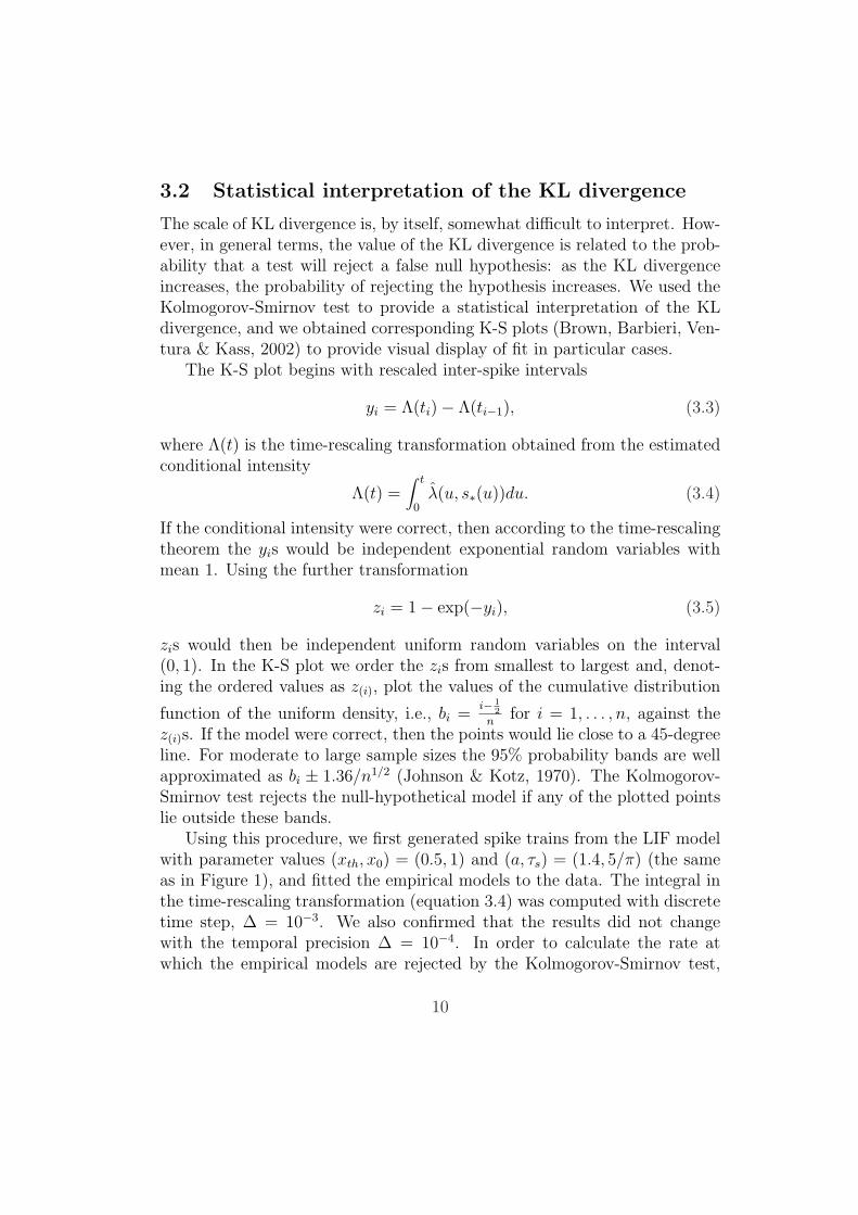
3.2 Statistical interpretation of the KL divergence

The scale of KL divergence is, by itself, somewhat difficult to interpret. How-ever, in general terms, the value of the KL divergence is related to the prob-ability that a test will reject a false null hypothesis: as the KL divergenceincreases, the probability of rejecting the hypothesis increases. We used theKolmogorov-Smirnov test to provide a statistical interpretation of the KLdivergence, and we obtained corresponding K-S plots (Brown, Barbieri, Ven-tura & Kass, 2002) to provide visual display of fit in particular cases.

The K-S plot begins with rescaled inter-spike intervals

yi = Λ(ti) − Λ(ti−1), (3.3)

where Λ(t) is the time-rescaling transformation obtained from the estimatedconditional intensity

Λ(t) =∫ t

0λ(u, s∗(u))du. (3.4)

If the conditional intensity were correct, then according to the time-rescalingtheorem the yis would be independent exponential random variables withmean 1. Using the further transformation

zi = 1 − exp(−yi), (3.5)

zis would then be independent uniform random variables on the interval(0, 1). In the K-S plot we order the zis from smallest to largest and, denot-ing the ordered values as z(i), plot the values of the cumulative distribution

function of the uniform density, i.e., bi =i− 1

2

nfor i = 1, . . . , n, against the

z(i)s. If the model were correct, then the points would lie close to a 45-degreeline. For moderate to large sample sizes the 95% probability bands are wellapproximated as bi ± 1.36/n1/2 (Johnson & Kotz, 1970). The Kolmogorov-Smirnov test rejects the null-hypothetical model if any of the plotted pointslie outside these bands.

Using this procedure, we first generated spike trains from the LIF modelwith parameter values (xth, x0) = (0.5, 1) and (a, τs) = (1.4, 5/π) (the sameas in Figure 1), and fitted the empirical models to the data. The integral inthe time-rescaling transformation (equation 3.4) was computed with discretetime step, ∆ = 10−3. We also confirmed that the results did not changewith the temporal precision ∆ = 10−4. In order to calculate the rate atwhich the empirical models are rejected by the Kolmogorov-Smirnov test,

10

we generated one hundred sets of repeated spike train trials, with varyingnumbers of trials—and, thus, varying total numbers of spikes (ISIs).

Figure 3 displays the rate of rejecting the models as a function of thenumber of spikes. The probability of rejecting the inhomogeneous Poissonprocess rises very fast, while it takes very much larger data sets to rejectthe m-IMI model and the TRRP. Figures 4(a) and (b) depict examples ofKolmogorov-Smirnov plots. With only 200 ISIs (part (a)), there is clearlack of fit of the Poisson model. With 7000 ISIs (part (b)) lack of fit ofthe TRRP becomes apparent, though the m-IMI model continues to fit themean-modulated LIF data. From Figure 3, in this example, roughly 104 ISIsare necessary to reject the TRRP with probability 0.8.

3.3 Time-varying input variance

Next we considered the input whose variance varies across time,

I(t) = σ(t)ξ(t), (3.6)

where

σ2(t) = 1 + a sint

τs

. (3.7)

This form could be interpreted as a signal in the variance of the input, ofwhich Silberberg et al considered the possibility in the cortex (Silberberg,Bethge, Markram, Pawelzik & Tsodyks, 2004). We set the parameter valuesof the LIF neuron to (xth, x0) = (0,−4) and τs = 10/π. We simulated theLIF model over the time interval 107∆ to generate a spike sequence, fit thethree probability models to data, and calculated the KL divergence.

The result of the KL divergence is displayed in Figure 5(a). In contrastto the case of time-varying mean input, the TRRP model fits the best tothe LIF neuron for this case. The value of the KL divergence of the TRRPmodel remains small even when the firing rate varies largely (Figure 5(b)).

Figures 5(c),(d) depict the rescaled interval distributions of the m-IMImodel and the TRRP model, respectively. The interval distributions of theTRRP model are almost identical even when the amplitude of the variancemodulation is changed whereas interval-distributions of the m-IMI modelshow variation.

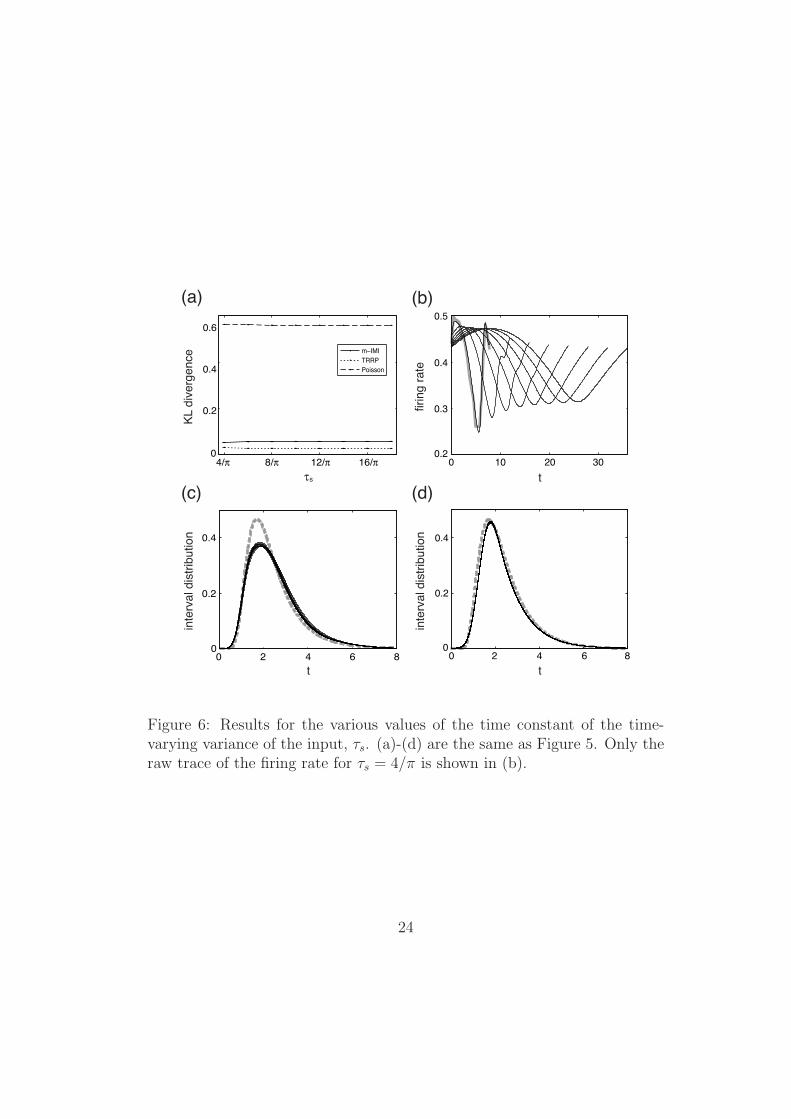
Figure 6 displays the results for various values of τs and fixed value of a.The parameter values of the LIF model in this figure are (xth, x0) = (0,−4)

11

and a = 0.8. It is confirmed from this figure that the results are qualitativelythe same as Figure 5. That is, the time-rescaled renewal process shows thebest agreement with the LIF neuron, and the best fitted interval distributionof the TRRP model is invariant for different values of τs.

3.4 Another example

So far we have examined the ability of the statistical models to accommodatedata from the LIF model driven by sinusoidal stimuli. We performed anothersimulation to confirm that the results are robust against different stimuli. Inthis example, we took f(t) to be a stimulus which has the form representedin Figure 7(a). Two cases were considered: the mean of the input to theLIF neuron varies across time, I(t) = f(t) + ξ(t), and the variance of theinput varies across time, I(t) = f(t)ξ(t). The parameter values of the LIFneuron were taken to be (xth, x0) = (0.5, 0). We simulated the LIF model togenerate sequences of spikes, fitted the m-IMI, TRRP, and the Poisson modelto data, and conducted the KS test. Figures 7(b) and (c) depict examplesof Kolmogorov-Smirnov plots. For the mean-modulated case (part (a)), thelack of fit of the TRRP model becomes apparent, though the m-IMI modelcontinues to fit the LIF model with 6000 ISIs. For the case of variance-modulated version (part (b)), however, the m-IMI model shows the lack offit with 1000 ISIs while the TRRP model continues to fit the LIF model.

4 Discussion

Our results examined the extent to which regularity and variability in spiketrains generated by a stimulus-driven LIF neuron could be captured by twoempirical models, the m-IMI model and the TRRP. Although the LIF modelinvolves a gross simplification of neuronal biophysics, it remains very widelyapplied in theoretical studies. This is one reason we investigated the perfor-mance of statistical models for stimulus-driven LIF spike trains. Our morefundamental motivation, however, was that LIF spike trains serve as a vehiclefor quantifying the similarity and differences between the m-IMI and TRRPspecifications of history effects. For a constant stimulus the LIF model be-comes stationary, generating a renewal process of spike trains, and the m-IMIand TRRP models become identical. The qualitative distinction between them-IMI and TRRP models in the non-stationary case may be understood by

12

considering the way the refractory period is treated: if, during an intervalof stationarity, for which the neuron has a constant firing rate, there is arefractory period of length δ, then when the firing rate changes the TRPPmodel will vary the refractory period away from δ while the m-IMI modelwill leave it fixed. More complicated effects, described under stationarityby a renewal process will, similarly, according to the two empirical models,either vary in time with the firing rate or remain time-invariant. Thus, it isperhaps not surprising that when a stimulus was applied to the mean of theLIF model, the fitted m-IMI model was closer than the TRRP model to thetrue LIF model that generated the data. The interval distribution plots inFigures 1 and 2 are consistent with this interpretation.

On the other hand, when the variance in the LIF model is temporallymodulated the renewal effects, such as the refractory period, become dis-torted in time. In this case we observed that the TRRP model fits betterthan the m-IMI model, and the interval distribution plot in Figure 5 showsless variation for the TRRP model than for the m-IMI model.

We also computed the power of the Kolmogorov-Smirnov (K-S) test as afunction of the number of spikes. We found that with relatively small samplesizes it can be easy to reject the hypothesis of Poisson firing, but very hardto distinguish m-IMI from TRRP models. This is demonstrated in the K-Splot of Figure 3(b). For the very large data set used in the K-S plot of Figure3(c), the m-IMI model provided a satisfactory fit while the TRRP did not.Overall, we would conclude first, that in most practical circumstances it isunlikely to matter much whether one uses the m-IMI model or the TRRP toproduce empirical fits to spike-train data but, second, m-IMI models wouldbe preferred when a mean-modulated LIF conception might be thought torepresent reality better than the variance-modulated version, and vice-versa.

Statistical models used to characterize such things as a receptive field, orthe effect of an oscillatory local field potential, must account for spike historyeffects. A successful approach has been to include m-IMI or TRRP terms ina loglinear model for the conditional intensity (Brown, Frank, Tang, Quirk& Wilson, 1998; Okatan, Wilson & Brown, 2005; Paninski, 2004; Truccolo,Eden, Fellows, Donoghue & Brown, 2005). As special cases of Equation 1, them-IMI and TRRP models studied here may be considered simplified versionsof the more realistic models used in the literature. Because we are focusingon history effects, we would anticipate that results for more complicatedsettings would be similar to those reported here.

13

A Derivation of the KL divergence

In this appendix we derive equation 2.9 from equation 2.7 under the condi-tions that pf and pq are periodically stationary with period T and E[n] → ∞as T ′ → ∞. Let {t1, . . . , tn} a sequence of spikes, θi = θ(ti) be the phase ofspike time ti and ui = ti − ti−1 be i-th inter-spike interval. The probabilitydensity of a spike sequence {t1, . . . , tn} in the time interval [0, T ′) for T ′ → ∞whose conditional ISI density is f(u|θ) is given by

pf (t1, . . . , tn) = Q(n)χ(θ(t1))f(t2 − t1|θ(t1)) · · · f(tn − tn−1|θ(tn−1))

= Q(n)χ(θ1)f(u2|θ1) · · · f(un|θn−1), (A.1)

where Q(n) is a probability distribution of spike count in the interval [0,∞).Equation (A.1) satisfies the normalization condition:

Q(0) + limT ′→∞

∞∑n=1

∫ T ′

0

∫ T ′

t1. . .

∫ T ′

tn−1

pf (t1, . . . , tn)dt1dt2 · · · dtn

= Q(0) +∞∑

n=1

Q(n)∫ T

0χ(θ1)dθ1

∫ ∞

0f(u2|θ1)du2 · · ·

∫ ∞

0f(un|θn−1)dun

=∞∑

n=0

Q(n) = 1. (A.2)

In equation 2.7, taking the limit of T ′ → ∞,∫ T ′

0

∫ T ′

t1· · ·

∫ T ′

tn−1

pf (t1, . . . , tn) logpf (t1, . . . , tn)

pq(t1, . . . , tn)dt1dt2 · · · dtn

→ Q(n)∫ T

0

∫ ∞

0· · ·

∫ ∞

0χ(θ1)

(n∏

i=2

f(ui|θi−1)

)n∑

j=2

logf(uj|θj−1)

q(uj|θj−1)dθ1du2 · · · dun

= Q(n)n∑

i=2

∫ T

0χ(θ1)

i−1∏j=2

∫ ∞

0f(uj|θj−1)duj

dθ1

×(∫ ∞

0f(ui|θi−1) log

f(ui|θi−1)

q(ui|θi−1)dui

) n∏k=i+1

∫ ∞

0f(uk|θk−1)duk

= Q(n)

n∑i=2

∫ T

0

∫ ∞

0χ(θi−1)f(ui|θi−1) log

f(ui|θi−1)

q(ui|θi−1)dθi−1dui

= Q(n)(n − 1)∫ T

0

∫ ∞

0χ(θ)f(u|θ) log

f(u|θ)q(u|θ)

dθdu, (A.3)

14

where we use

∫ T

0χ(θ1)

i−1∏j=2

∫ ∞

0f(uj|θj−1)duj

dθ1 =∫ T

0χ(θi−1)dθi−1. (A.4)

Substituting equation A.3 into equation 2.7 leads to

D(pf ||pq) = limT ′→∞

1

E[n]

∞∑n=1

Q(n)(n − 1)∫ T

0

∫ ∞

0χ(θ)f(u|θ) log

f(u|θ)q(u|θ)

dθdu

= limT ′→∞

(1 − 1 − Q(0)

E[n]

) ∫ T

0

∫ ∞

0χ(θ)f(u|θ) log

f(u|θ)q(u|θ)

dθdu

=∫ T

0

∫ ∞

0χ(θ)f(u|θ) log

f(u|θ)q(u|θ)

dθdu. (A.5)

B TRRP model

In this appendix we show that the rescaling function of the TRRP model,λ0(t), corresponds to the trial-averaged conditional intensity function, up toan arbitrary multiplicative constant. Let g0(u) be the hazard function of arenewal process and, to avoid transient start-time effects, suppose that therenewal point process starts from u = −∞. Let e∗(u) be the event time priorto u. By the renewal theorem (Theorem 4.4.1 in Daley & Vere-Jones, 2003),the expectation of g0(u − e∗(u)) is constant:

Eg0(u − e∗(u)) = c (B.1)

for some positive c. Now transform time from u to t with a monotonic time-rescaling function t = Λ−1

0 (u), where Λ0(t) is given by Equation 2.6. By thechange of variables formula, the conditional intensity as a function of timet is given by Equation 2.5. Taking expectations of both sides and applyingEquation B.1 we get

E[λ(t, s∗(t))] = λ0(t)c. (B.2)

If we replace g0(t) with h(t) = g0(t)/c then λ0(t) becomes the expected(trial-averaged) conditional intensity function. This is convenient becauseλ0(t) may then be estimated by pooling data across trials, i.e., by smoothingthe PSTH.

15

Acknowledgment

We thank Taro Toyoizumi for helpful discussions.

References

Barbieri, R., Quirk, M. C., Frank, L. M., Wilson, M. A., & Brown, E. N.(2001). Construction and analysis on non-Poisson stimulus-responsemodels of neural spiking activity. Journal of Neuroscience Methods,105, 25-37.

Brown, E. N., Barbieri, R., Ventura, V., Kass, R. E., & Frank, L. M. (2002).The time-rescaling theorem and its application to neural spike traindata analysis. Neural Computation, 14, 325-346.

Brown, E. N., Frank, L. M., Tang, D., Quirk, M. C., & Wilson, M. A.(1998). A statistical paradigm for neural spike train decoding appliedto position prediction from ensemble firing patterns of rat hippocampalplace cells. Journal of Neuroscience, 18, 7411-7425.

Burkitt, A. N., & Clark, G. M. (2001). Synchronization of the neural responseto noisy periodic synaptic input. Neural Computation, 13, 2639-2672.

Cox, D., R., & Lewis, P. A. W. (1972). Multivariate point processes. In Proc.6th Berkeley Symp. Math. Statist. Prob. 3, (pp.401-448). Berkeley: Uni-versity of California Press.

Daley, D., & Vere-Jones, D. (2003). An introduction to the theory of pointprocesses. New York: Springer-Verlag.

Dayan, P., & Abbott, L. F. (2001). Theoretical neuroscience. Cambridge,AM: MIT Press.

de Boor, C. (2001). A practical guide to splines (Revised Ed.). New York:Springer.

Gerstner, W., & Kistler, W. M. (2002). Spiking neuron models. Cambridge:Cambridge University Press.

Iyengar, S., & Mullowney, P. (2007). Inference for the Ornstein-Uhlenbeckmodel for neural activity. preprint.

Johnson, A., & Kotz, S. (1970). Distributions in statistics: Continuous uni-variate distributions. Vol. 2. New York: Wiley.

Kass, R. E., & Ventura, V. (2001). A spike-train probability model. NeuralComputation, 13, 1713-1720.

16

Kass, R. E., Ventura, V., & Brown, E. N. (2005). Statistical issues in theanalysis of neuronal data. Journal of Neurophysiology, 94, 8-25.

Koch, C. (1999). Biophysics of computation: Information processing in singleneurons. New York: Oxford University Press.

Koyama, S., & Shinomoto, S. (2005). Empirical Bayes interpretations ofrandom point events. Journal of Physics A: Mathematical and General,38, L531-L537.

Lansky P., Sanda, P., & He J. (2006). The parameters of the stochastic leakyintegrate-and-fire neuronal model. Journal of Computational Neuro-science, 21, 211-223.

McCullagh, P., & Nelder, J. A. (1989). Generalized linear models (2nd ed.).New York: Chapman and Hall.

Okatan, M., Wilson, M. A., & Brown, E. N. (2005). Analyzing functionalconnectivity using a network likelihood model of ensemble neural spik-ing activity. Neural Computation, 17, 1927-1961.

Paninski, L. (2004). Maximum likelihood estimation of cascade point-processneural encoding models. Network: Computation in Neural Systems, 15,243-262.

Paninski, L., Pillow, J. W., & Simoncelli, E. P. (2004). Maximum likelihoodestimation of a stochastic integrate-and-fire neural encoding model.Neural Computation, 16, 2533-2561.

Plesser, H. E., & Geisel, T. (1999). Markov analysis of stochastic resonancein a periodically driven integrate-and-fire neuron. Physical Review E,59, 7008-7017.

Reich, D. S., Victor, J. D., & Knight, B. W. (1998). The power ratio andinterval map: Spiking models and extracellular recordings. Journal ofneuroscience, 18, 10090-10104.

Silberberg, G., Bethge, M., Markram, H., Pawelzik, K., & Tsodyks, M.(2004). Dynamics of population rate codes in ensembles of neocorti-cal neurons. Journal of Neurophysiology, 91, 704-709.

Snyder, D. L., & Miller, M. I. (1991). Random point processes in time andspace (2nd Ed.) New York: Springer-Verlag.

Truccolo, W., Eden, U. T., Fellows, M. R., Donoghue, J. P., & Brown, E. N.(2005). A point process framework for relating neural spiking activity tospiking history, neural ensemble, and extrinsic covariate effects. Journalof Neurophysiology, 93, 1074-1089.

Tuckwell, H. C. (1988). Introduction to theoretical Neurobiology. Cambridge:Cambridge University Press.

17

van Kampen, N. G. (1992). Stochastic processes in physics and chemistry(2nd ed.). Amsterdam: North-Holland.

18

0 0.5 1 20

0.1

0.2

0.05

0 0.5 1 20

1

0 0.5 1 20

0.5

0 2 6 100

1

2

3

4

a

KL d

iverg

en

ce

t

1.5

t t

firing

ra

te

inte

rval dis

trib

utio

n

inte

rval dis

trib

utio

n

(a) (b)

(c) (d)

1.5 4 8

1.5

0.5

1.5

1.5

1

0.15

m−IMI

TRRP

Poisson

Figure 1: Results for the case that the mean input is varying in time. (a)The KL divergence as a function of the amplitude of the mean input, a.Solid line, dotted line and dashed lines represent the KL divergence of them-IMI model, the TRRP model and the inhomogeneous Poisson process, re-spectively. The mean and the standard error at each point were calculatedwith ten repetitions. The KL divergence of the inhomogeneous Poisson pro-cess is much larger than that of the m-IMI model and the TRRP model.(b) The instantaneous firing rates of the LIF neuron for various values of a.Thin solid lines represent the instantaneous firing rates of the LIF model,and the gray thick lines are raw traces. The amplitude of the instantaneousfiring rate is increasing as a is increasing. (c) Solid lines represent rescaledinterval distributions of the m-IMI model for various values of a, which areobtained from the recovery function by equation 3.2. The gray dashed lineis the interval distribution of the LIF model for a = 0. (d) Same as (c) forthe TRRP model. The rescaled interval distributions both in (c) and (d) aredeparting from the interval distribution of the LIF model as a is increasing,but it shows less variation for the m-IMI model than for the TRRP model.

19

2/π 4/π 6/π 8/π0

0.05

0.1

0.15

0 0.5 1 1.5 20

0.5

1.5

0 0.5 1 1.5 20

0.5

1

0 10 15 200

0.5

1.5

2

KL d

iverg

ence

t

t t

firing r

ate

inte

rval dis

trib

ution

inte

rval dis

trib

ution

(a) (b)

(c) (d)τs

5

1

1

1.5

10/π

m−IMI

TRRP

Poisson

Figure 2: Results for various values of the time constant of the time-varyingmean input, τs. (a)-(d) are the same as Figure 1.

20

102

103

104

0

0.2

0.4

0.6

0.8

1

Number of ISIs

Pro

babili

ty o

f re

jecting

a m

ode

l

m−IMI

TRRP

Poisson

Figure 3: The probability of rejecting probability models as a function ofthe number of ISIs. Solid line, dotted line and dashed represent the m-IMImodel, the TRRP model and the inhomogeneous Poisson process. The meanand the standard error at each point were calculated with 10 repetitions.With relatively small sample sizes it can be easy to reject the hypothesis ofPoisson firing, but very hard to distinguish m-IMI model from TRRP models.

21

0 0.5 10

0.5

1

0 0.5 10

0.5

1

(a)

(b)

m−IMI

TRRP

Poisson

m−IMI

TRRP

Poisson

Figure 4: (a) The Kolmogorov-Smirnov plot using 200 ISIs showing the Pois-son model does not fit, but the two other models do. (b) Same as (a) using7000 ISIs showing that the m-IMI model fits, but the two other models donot.

22

0 0.2 0.4 0.6 0.80

0.2

0.4

0.6

0 2 4 6 80

0.2

0.4

0 2 4 6 80

0.2

0.4

0 5 10 15 200.2

0.3

0.4

0.5

a

KL d

ive

rge

nce

t

t t

inte

rva

l d

istr

ibu

tio

n

inte

rva

l d

istr

ibu

tio

n

(a) (b)

(c) (d)

firin

g r

ate

m−IMI

TRRP

Poisson

Figure 5: Results for the case that the input variance is varying in time.(a)-(d) are the same as Figure 1. Only the raw trace of the firing rate fora = 0.9 is shown in (b). In this case the KL divergence of the TRRP model isthe smallest among three models, and the interval distribution for the TRRPmodel shows less variation than for the m-IMI model.

23

4/π 8/π 12/π 16/π0

0.2

0.4

0.6

0 2 4 6 80

0.2

0.4

0 2 4 6 80

0.2

0.4

0 10 20 30

0.3

0.4

0.5

KL d

iverg

ence

t

t t

firing r

ate

inte

rval dis

trib

utio

n

inte

rval dis

trib

utio

n

(a) (b)

(c) (d)τs

m−IMI

TRRP

Poisson

0.2

Figure 6: Results for the various values of the time constant of the time-varying variance of the input, τs. (a)-(d) are the same as Figure 5. Only theraw trace of the firing rate for τs = 4/π is shown in (b).

24

m−IMI

Poisson

TRRP

t

(a)

(b) (c)

0 0.5 10

0.5

1

m−IMI

Poisson

TRRP

0 0.5 10

0.5

1

100 20 30 40 500

1

2

3

f(t)

Figure 7: (a) The shape of the stimulus, f(t). (b) Kolmogorov-Smirnov plotusing 6000 ISIs showing that the m-IMI model fits, but the two other modelsdo not for the mean-modulated stimulus. (c) Same as (b) using 1000 ISIsshowing that the TRRP model fits, but the two other models do not for thevariance-modulated stimulus.

25