SPATIAL DECOMPOSITION OF POVERTY IN RURAL …jed.or.kr/full-text/39-4/4.pdf · SPATIAL DECOMPOSITION OF POVERTY IN RURAL NIGERIA 79 Geographically-based theories of poverty calls

JOURNAL OF ECONOMIC DEVELOPMENT 77 Volume 39, Number 4, December 2014

SPATIAL DECOMPOSITION OF POVERTY IN RURAL NIGERIA:

SHAPLEY DECOMPOSITION APPROACH

OLUWAKEMI ADEOLA OBAYELU

*

Department of Agricultural Economics, University of Ibadan, Nigeria

Poverty is largely a rural phenomenon in sub-Saharan Africa and the key contributors to poverty are low mean per capita income and its inequitable distributions. The contribution of mean income and inequality to spatial variations in rural poverty were investigated in this study using the 2003/04 National Living Standard Survey by the National Bureau of Statistics (NBS). The data were analyzed using descriptive statistics and Shapley Decomposition (SD) techniques. Results showed that across the GPZs, the contributions of mean income to change in poverty rates were higher than inequality (Ly) for both incidence of poverty ( 0P ) and poverty gap ( 1P ). On the other hand, the contribution of mean income

to change in severity of poverty ( 2P ) was higher than Ly in North-East ( μ 0.0530;

Ly -0.0334); North-West ( μ 0.0844; Ly 0.0429); South-East ( μ -0.0505;

Ly -0.0136); South- South ( μ -0.0254; Ly -0.0048); South-West ( μ -0.0450;

Ly -0.0201). However, inequality contributed more than mean income in North-Central

( μ 0.0184; Ly 0.0240). The marginal contributions of within-GPZs inequality to

poverty indices were higher than between-GPZs inequality. Keywords: Poverty, Inequality, Decomposition, Shapley, Rural JEL classification: I32

1. INTRODUCTION Poverty in a given country and at a given point of time is fully determined by the rate

of change in the mean income of the population and the change in the distribution of income (Bourguignon, 2004). The modern theoretical approach to understanding poverty considers the income dimension as the core of most poverty-related problems. Poverty may stem from changes in average income or changes in the distributed income. This implies that equitable distribution of income would increase the probability of the poor having access to basic needs (such as food consumption, housing, health, education, et

* The author would like to thank an anonymous referee for very useful comments and suggestions.

OLUWAKEMI ADEOLA OBAYELU 78

cetera). On the other hand, increasing per capita income without redistributing part of the wealth created affects the performance of the economy and marginalizes even more the lower per centile of population. This, consequently, has a negative impact on poverty reduction (Molini, 2005). Thus, the welfarist approach establishes a close positive relationship between per capita income (PCI) and the measures of well-being. However, per capita income does not so much determine capabilities but how it is distributed. The argument for economic growth as a pre-requisite for poverty reduction is because it increases mean income and narrowing of income distribution (Ajakaiye and Adeyeye, 2001).

The poverty triangle proposed by Bourguignon (2004) illustrates how changes in distribution and changes in mean income determine the extent to which a country reduces poverty (Figure 1). A change in the distribution of income can be decomposed into two effects. First, there is the effect of a proportional change in all incomes that leaves the distribution of relative income unchanged, i.e., a mean income effect. Second, there is the effect of a change in the distribution of relative incomes which, by definition, is independent of the mean, i.e., a distributional effect (Datt and Ravallion, 1992; Kakwani, 1993). This movement thus corresponds to the change in the distribution of ‘relative’ income, or the ‘distribution’ effect. If the distribution of income does not change, then poverty reduction is only possible with growth. Without growth in mean income, redistribution of income in favour of the poor is the only way to reduce poverty. In other words, the incomes of the non-poor would have to fall in order for the incomes of the poor to rise. In practice, a change in poverty comes about through some combination of a change in average incomes and a change in the distribution of income. According to Bourguignon, the real challenge to establishing a development strategy for reducing poverty lies in the interaction between distribution and growth, and not in the relationship between poverty and growth on the one hand and poverty and inequality on the other, which are essentially arithmetic.

Note: Bourguignon (2004).

Figure 1. The Poverty Triangle

SPATIAL DECOMPOSITION OF POVERTY IN RURAL NIGERIA

79

Geographically-based theories of poverty calls attention to the fact that people, institutions, and cultures in certain areas lack the objective resources needed to generate well-being and income, and that they lack the power to claim redistribution. Shaw (1996) opines that space is not a backdrop for capitalism but rather is restructured by it and contributes to the system’s survival. The geography of poverty is therefore a spatial expression of the capitalist system. A notable aspect of poverty in Nigeria is that the poor are often concentrated in communities without basic services. In 1998 and 2004, The North West, North East and North Central geopolitical zones (GPZs) have the highest aggregate poverty rates in descending order while the South West, South East, and South South GPZs have the lowest aggregate poverty rates in ascending order. These six GPZs also reflect varying ecologies and climates, along with differing population characteristics. The reductions in the poverty rates for rural households in the southern zones are far greater than those achieved by their northern counterparts and it could be concluded that poverty is more prevalent in the northern zones than in the southern zones (Omonona, 2010).

Geographic differences have also played a role in the divide. Owing to its nearness to the Sahara Desert, Nigeria’s North is susceptible to drought and climate change (Adejuwon, 2008). From the economic point of view, the North GPZs has a disproportionately higher percentage of subsistence households than the South GPZs. The combination of extensive poverty, food insecurity, poor health, poor infrastructure, and low levels of education in the North has resulted in livelihoods less easily adaptable to change (Asadurian et al., 2006; Adejuwon, 2008; Agunwamba et al., 2009). In addition, the healthcare financing in the north is relatively lower than in the south, followed by considerable poor health status, with heavy dependence on the households in both regions. The expenditure share of households in the north is also proportionally disproportionate, because of the high poverty incidence vis-a-vis public providers (Lawanson and Olaniyan, 2013).

Although few studies have highlighted the decomposition of income poverty in Nigeria (Oyekale et al., 2006; Araar and Awoyemi, 2006; Uneze and Adeniran, 2014; Adigun and Awoyemi, 2014), we still lack understanding of spatial poverty decomposition in rural Nigeria. This is especially important because the majority of the poor reside in the rural areas where most of the people and national resources are located and thus making rural poverty a major driver of aggregate poverty in Nigeria (Osinubi, 2003; Ogwumike and Akinnibosun, 2013). This study deviates from previous studies on poverty in a number of ways. First, in the specificity of the study area which is rural Nigeria. Second, the study also estimated the marginal contribution of inequality to poverty in the six geopolitical zones of rural Nigeria.

2. METHODOLOGY The data used for this study were from the 2003/04 Nigeria Living Standard Survey


(NLSS) data from the National Bureau of Statistics (formerly known as the Federal Office of Statistics). The sample design was a two-stage stratified sampling. The first stage involved the selection of 120 Enumeration areas (EAs) in each of the 36 states and 60 EAs at the Federal Capital Territory (FCT). The second stage was the random selection of five housing units from each of the selected EAs. A total of 21,900 households were randomly interviewed across the country with 19,158 households having consistent information (NBS, 2005). For the purpose of this study, the secondary data was first stratified into rural and urban sectors. The second stage was the stratification of the rural area based on the six geo-political zones of Nigeria viz: South West, South East, South South, North Central, North East and North West. The next stage involved the selection of all the sampled rural households in each of the geo-political zones. The data set provides detailed records on household expenditure (which was used as a proxy for household income) and household characteristics. However, 14,514 rural households whose responses were consistent were used for analyses in this study.

2.1. Poverty Decomposition Framework The relative poverty line is estimated based on the expenditure profile of respondents

on basic needs (food and non-food items). However, the total household per capita expenditure (PCE) is used as proxy of standard of living. This method has been applied by several authors (World Bank, 1996; Canagarajah et al., 1997; Olaniyan, 2002). Here, the total PCE is the sum of cash expenditure on consumption of food and non-food items relative to individual household size.

HouseholdsofNumberTotal

PCETotalMOCHHEPCEMean )(

The non-poor threshold is the region greater than two-thirds of MPCHHE while the

moderate poverty line ranges from one-third to two-thirds of MPCHHE; and The core-poor threshold is the region less than one-third of MPCHHE. This study adopted Foster, Greer and Thorbecke (1984) approach to estimate the incidence, depth and severity of poverty in the study area. The FGT indices are calculated by taking the proportional shortfall in expenditure for each poor household and normalising the sum by the population size.

2.2. Poverty Decomposition In this study, poverty rate was calculated by comparing the total expenditure of

every household with the corresponding poverty line. Suppose income x of an individual is a random variable with the distribution function )(xF . Let z denote the poverty line,


81

the threshold expenditure below which one is considered to be poor. Then )(zF is the

proportion of individuals (or families) below the poverty line. This measure, widely used as a poverty measure, is called the headcount ratio. Here, the national poverty level can be thought of as a function of three factors: regional disparities in average level of consumption denotes by µ; intraregional inequalities denotes as L; and the subsistence level for a single adult, denoted by z, which reflects regional price variations. Thus, we have poverty as a function of these three components

),,( zLμP . (1)

This indicates that regional poverty levels are largely determined by three factors:

income inequalities, as captured by the Lorenz curve, mean income per capita, and poverty line. It is therefore worth exploring the import of each of these proximate sources of poverty if only to confirm or counter, the common presumption that average income is the dominant influence on poverty (Kolenikov and Shorrocks, 2005).

Assuming a fixed poverty line, the poverty level in any region is given by

),(, 00 LαPLz

μP

, (2)

where 0α (i.e., z

μ) is the normalised mean income level of the region and 0L is the

Lorenz curve representing the relative distribution of income in the region. Similarly, the poverty level of the country as a whole is given by

),( 11 LαP , (3)

where 1α is the mean income level of the country and 1L is the Lorenz curve

representing the income distribution of the country. We shall employ a decomposition technique based on the Shapley value in cooperative game theory to quantify the explanatory power of these factors to poverty in each region. Let us use the subscript “1” to denote the national income distribution, following Datt and Ravallion (1992) and Zhang and Wan (2005), then the difference between poverty at the national and regional levels is simply:

),(),(Δ 0011 LαPLαPP . (4)

Thus, the total difference between the regional and the national poverty rates arises

from the differences in two factors: the average income α and the distribution of income L. To separate the effects of these two factors, Datt and Ravallion (1992) defines


the contribution of income differences as:

),(),()(Δ 0 rrii LαPLαPαP , (5)

and the contribution of inequality differences as

),(),()(Δ 0LαPLαPLP riri , (6)

where r can be either i or 0 as long as it is consistent across the two equations. The problem with this decomposition is that )(Δ αPi and )(Δ LPi do not add up to iPΔ . In

cases where the discrepancy is large, the decomposition would leave unexplained the bulk of the difference in poverty. Further, the decomposition results vary with the choice of the reference point r, and there is no guidance on how to choose one over the other.

The Shapley decomposition procedure follows Kolenikov and Shorrocks (2005). To find the Shapley value of the contribution to iPΔ by regional differences in mean

income and inequality amounts to considering the four possible sequences of replacing

0α , and 0L with iα , and iL , and averaging the marginal effects of )(Lα over the

four sequences. ),( 01 LαP tells us what would have been a region’s poverty level if the

region’s mean had been the national mean, without any change in its distribution of income. On the other hand, ),( 10 LαP tells us what would have been a region’s poverty

level if there had been no change in the region’s mean income level but its distribution of income had been the income distribution at the national level.

Thus, we can decompose variation of the FGT index into PCE effect α , and inequality L, effects as follows: 21 CC where 1C is the expenditure component and

2C is the inequality component. The expenditure component is expressed as:

)]),(),([)],(),(([2

1101100011 LαPLαPLαPLαPC . (7)

The first component gives the difference in poverty due to changes in the mean

expenditure when distribution of expenditure is held fixed at the regional level. The second component gives the difference in poverty due to changes in the mean income when distribution is held fixed at the national level.

Similarly, the difference between the national and region poverty levels arising purely from the difference between their distributions of expenditure is given by:

)]),(),([)],(),(([2

1011100102 LαPLαPLαPLαPC . (8)

The first component gives the difference in poverty due to changes in the distribution


83

of expenditure when mean expenditure is held fixed at the regional level. The second component gives the difference in poverty due to changes in the distribution of expenditure, when mean expenditure is held fixed at the national level.

2.3. Marginal Contributions of Within and Between GPZs Inequalities The region is not, of course, the only factor that accounts for differences in living

standards: there are typically wide disparities in incomes within, as well as between, regions. Here, the marginal contribution of a given component refers to the variation in poverty index after adding the latter to the complement components set. We follow Araar (2006), to simulate at the margin the impact of the inequalities between the regions on the national poverty and the impact of its corresponding within the region inequality on the national poverty. We again start with the popular decomposable FGT index. In which case we have the total poverty as:

),,(),,(1

LzYPφLzYP gg

G

gg

, (9)

where G is the number of mutually exclusive subgroups in the total population, and g is the population of group g and gP is the poverty measure for group g, gφ is the

proportion of group g in the population, gY is the total expenditure of group g, z is the

poverty line and L measures parameters of the Lorenz curve. The total poverty is the sum of the contributions of each region or group poverty to the national poverty P.

In order to simulate at the margin the impact of the within region disparity on total poverty we examine the situation where the total inequality is removed from the total poverty. This corresponds to the situation where each household has the average expenditure of its region, denoted by gμ . Formally we have:

),,(),,(1

** LzμPφLzYP gg

G

gg

. (10)

It follows that at the margin the difference between (3.11) and (3.12) gives the total

contribution of the regional disparities (CRD) to the national poverty which equals to:

*PPCRD . (11) The contribution of group/region g to the national disparity also equals to:

)( *PPφCRD gg , (12)


where gφ is the proportion of region g in the total population.

Further, to eliminate the inter region inequality and to calculate the contribution at the margin of the intra-region inequality on poverty, we will use a vector of expenditure where each household has its income multiplied by the ratio gμμ / . With this new

expenditure vector, the average of the expenditure of each region equals to μ . Thus, the

FGT index of within group is denoted by:

Lz

μ

μPφLzYP

gg

G

gg ,,),,(

1

**** . (13)

Therefore, the contribution of the within regional disparities equals to:

**PPWRD . (14) It is to be noted that if this procedure gives us an idea on the contribution of each of

the two factors, this approach overestimates their contributions such that:

BWP CCC . (15)

To avoid this flaw, we use the Shapley approach by keeping the same rules for eliminating each of the between and within group factors. Similarly, the contribution of the group g to the within group disparities equals to:

)( **PPφWRDg gi . (16)

The use of the Shapley approach to estimate the expected marginal contributions of the within and between regional inequalities to the total poverty is given as:

)],,()()(),([2

1LzμPWPBPBWPC S

W ,

)],,()()(),([2

1LzμPBPWPBWPC S

B ,

where )],,(),( LzYPBWP and, (17)

),()( LzμPφBP ggg , and

L

μ

μYzPφWP

gggg ,,)( .


85

SWC and S

BC are the expected contributions of within and between groups

inequalities to national poverty respectively. The decomposition facility in the DAD Software developed by Duclos and Araar,

(2006) provides opportunity to decompose these factors.

3. RESULTS 3.1. Distribution of Household Per Capita Expenditure by Percentile Results in Table 1 show that the mean of the topmost percentile was about 12 times

greater than the lowest percentile. This indicates a high gap in income level in rural area. The results further reveal that at the lowest percentile (5 percentile) of expenditure distribution, South West has the highest (₦10695.6183) PCE while North Central zone has the least (₦4492.7473). This reveals inequitable in income distribution in rural Nigeria. Among the middle income earners (50 percentile), South West has the highest (₦48, 498.1948) mean PCE while North East records the least (₦15920.9774). At the topmost percentile (95 percentile), South East has the highest mean PCE (₦98616.7637), closely followed by South West (₦97117.3451); while North West records the least (₦ 45647.7249). This indicates that standard of living in South West is the best of all the zones while it is worst in North Central.

Table 1. Distribution of Geopolitical Zones by Income Percentiles ZONES PERCENTILES

5 10 25 50 75 90 95 South South 8036.69 10059.35 15087.96 25205.83 41177.29 63786.35 85589.14 South East 10203.09 13101.47 20070.14 31146.43 47973.66 73864.53 98616.76 South West 10695.62 13338.46 20273.82 31325.75 48498.20 71074.73 97117.35

North Central 4492.75 6004.73 10740.80 18750.06 30846.54 48668.67 66803.43 North East 6055.64 7940.11 11596.22 17399.71 26794.43 40072.98 51723.09 North West 5869.44 7425.36 10731.81 15920.98 23052.38 34496.53 45647.73

National 6183.43 8263.99 12925.29 20877.98 34385.82 54488.47 73869.52 The estimation of the poverty line presented in Table 2 shows that the mean PCE for

Nigeria is ₦31, 764.00 and the moderate poverty line is ₦21, 176.03. The result shows that about half (51 per cent) of the rural households are poor and an average poor household would need to attain a per capita income level of about ₦1, 974 to get out of poverty. There is also a fairly large ( 2P 0.1030 inequality in income distribution of the

rural households.


Table 2. Estimation of National Poverty Line Variables Estimates

Mean PCEXPDR ₦ 31, 764.06 Core Poverty Line ₦ 10, 588.02

Moderate Poverty Line ₦ 21, 176.03 Poverty incidence (Rural) 0.5053

Poverty depth (Rural) 0.1974 Poverty severity (Rural) 0.1030

3.2. Spatial Profile of Incidence of Poverty in Rural Nigeria Figures in Table 3 reveal that North West had the highest incidence of rural poverty

( 0P 0.6925). This is closely followed by the North East ( 0P 0.6069) and the North

Central ( 0P 0.5598). These zones contribute 29.5 percent, 22.6 per cent and 21 per

cent respectively to overall incidence of rural poverty. This indicates that together, the North West, North East and North Central contribute 73.1 per cent to overall rural poverty incidence. This corroborates the findings of Minot et al., (2003) that poverty is more pronounced in remote and dry regions of Vietnam. Further, South West records the lowest incidence of poverty ( 0P 0.2699) and the lowest relative contribution of 4.4 per

cent to overall poverty. This is followed by the South East with poverty incidence and relative contribution of 28 per cent and 8 per cent respectively. This shows that the proportion of the poor in North West is about thrice that of South West. The implication of this is that majority of the rural poor reside in the northern GPZs of Nigeria, which is a savannah belt. Thus, poverty may be as a result of returns to variations in natural assets and geo-climatic endowments.

Of the thirty-six states, the proportion of rural poor is highest in Kwara, Kogi, Jigawa, Lagos and Kebbi states in a descending order while the least incidence of rural poverty was observed in Oyo, Osun and Imo in an ascending order. Thus, the proportion of the poor in Kwara was about seven times that of Oyo. This suggests that variations are due to spatial differences and level of economic development.

Table 3. Spatial Analysis of Incidence of Poverty (Headcount) in Rural Nigeria GPZs/States Estimate Proportion Absolute Contribution Relative Contribution

ALL 0.5053 South South 0.4198 0.1628 0.0684 0.1353 AkwaIbom 0.3755 0.0316 0.0119 0.0235 Bayelsa 0.2236 0.0327 0.0073 0.0145 CrossRiver 0.4943 0.0303 0.0150 0.0296 Delta 0.5362 0.0238 0.0128 0.0252


87

Edo 0.5297 0.0243 0.0129 0.0255 Rivers 0.4252 0.0203 0.0086 0.0170

South East 0.2803 0.1620 0.0454 0.0899 Abia 0.2500 0.0278 0.0070 0.0138 Anambra 0.2076 0.0325 0.0066 0.0134 Ebonyi 0.4506 0.0349 0.0157 0.0311 Enugu 0.2845 0.0334 0.0095 0.0188 Imo 0.1942 0.0337 0.0065 0.0128

South West 0.2699 0.0822 0.0222 0.0439 Ekiti 0.2891 0.0145 0.0042 0.0083 Lagos 0.8182 0.0023 0.0019 0.0037 Ogun 0.2735 0.0154 0.0042 0.0083 Ondo 0.3370 0.0249 0.0084 0.0166 Osun 0.1515 0.0136 0.0021 0.0041 Oyo 0.1265 0.0114 0.0014 0.0029

North Central 0.5598 0.1896 0.1061 0.2100

Benue 0.3957 0.0291 0.0115 0.0228

Kogi 0.8361 0.0336 0.0281 0.0556

Kwara 0.8842 0.0196 0.0174 0.0344

Nassarawa 0.4143 0.0309 0.0128 0.0254

Niger 0.5107 0.0322 0.0165 0.0326

Plateau 0.4651 0.0316 0.0147 0.0290

FCT 0.4144 0.0125 0.0052 0.0102

North East 0.6069 0.1883 0.1143 0.2261

Adamawa 0.6336 0.0320 0.0203 0.0401

Bauchi 0.7251 0.0354 0.0256 0.0507

Borno 0.5479 0.0230 0.0126 0.0250

Gombe 0.6536 0.0298 0.0195 0.0386

Taraba 0.4027 0.0354 0.0143 0.0282

Yobe 0.6730 0.0327 0.0220 0.0435

North West 0.6925 0.2151 0.1490 0.2948

Jigawa 0.8302 0.0361 0.0300 0.0593

Kaduna 0.4354 0.0245 0.0107 0.0211

Kano 0.5487 0.0234 0.0128 0.0254

Katsina 0.6099 0.0320 0.0195 0.0386

Kebbi 0.8024 0.0345 0.0277 0.0548

Sokoto 0.7530 0.0287 0.0216 0.0428

Zamfara 0.7428 0.0359 0.0267 0.0528

Source: Estimated from NLSS (2003/2004).


3.3. Spatial Profile of Depth of Poverty in Rural Nigeria Spatial variations of depth of poverty across GPZs and states in rural Nigeria are

presented in Table 4. As expected, rural poverty gap index was highest ( 1P 0.2781) in

North West and lowest ( 1P 0.0835) in South West indicating that a typical poor rural

household in the North West would require about thrice the amount of resources required by their counterparts in the SouthWest to get out of poverty. This further confirms that the rural South West not only had the lowest proportion of the poor but is also were more developed economically than other zones. This is also because past South Western governments, through various policies, had emphasised more on investment in formation of capital assets than other zones. Leading among such policies are free education, free health services, agricultural credits, formation of cooperative societies as well as community and rural development. Further, the relative contributions of the zones to poverty gap in a descending order are North West (0.3030), North Central (0.2390), North East (0.2295), South South (0.1229), South East (0.0709) and South West (0.0348) suggesting that the while the North West has the highest (30 per cent) contribution to depth of rural poverty in Nigeria, the South West has the least (3.5 per cent).

Among the states, Kwara has the highest ( 1P 0.5322) depth of rural poverty index

while Oyo records the least ( 1P 0.0379) implying that poor rural households in Kwara

would need fourteen fold of increase in per capita income their counterparts in Oyo State need to alleviate their poverty. Notably, the depth of rural poverty in Kogi, Lagos and Jigawa are also on the high side representing 0.4940, 0.4247 and 0.3894 respectively. The highest relative contribution of the states to rural poverty gap in a descending order are Kogi (8.4 per cent), Jigawa (7.1 per cent), Kebbi (5.6 per cent), Zamfara (5.4 per cent) and Kwara (5.3per cent) and Bauchi (5.1 per cent). As expected, the least relative contributions are from Oyo (0.22 per cent) and Osun (0.28 per cent). However, contrary to expectation, Lagos contributes only 0.4 per cent. This is explained by the low proportion of the overall rural households residing in Lagos resulting from increasing rural-urban drift as well as urbanisation. Urban Lagos is the commercial centre in Nigeria with a seaport, an international airport and highest concentration of both micro- and macro-enterprises.

Table 4. Spatial Analysis of Poverty Depth (Gap) in Nigeria GPZs/States Estimate Proportion Absolute Contribution Relative Contribution

All 0.1974 South South 0.1490 0.1628 0.0243 0.1229 AkwaIbom 0.1198 0.0316 0.0038 0.0191 Bayelsa 0.0832 0.0327 0.0027 0.0138 CrossRiver 0.1775 0.0303 0.0054 0.0272


89

Delta 0.1913 0.0238 0.0045 0.0230 Edo 0.1930 0.0243 0.0047 0.0238 Rivers 0.1557 0.0203 0.0032 0.0160 South East 0.0864 0.1620 0.0140 0.0709 Abia 0.0753 0.0278 0.0021 0.0106 Anambra 0.0515 0.0325 0.0017 0.0085 Ebonyi 0.1598 0.0349 0.0056 0.0282 Enugu 0.0852 0.0334 0.0028 0.0144 Imo 0.0541 0.0337 0.0018 0.0091 South West 0.0835 0.0822 0.0069 0.0348 Ekiti 0.0793 0.0145 0.0012 0.0058 Lagos 0.4247 0.0023 0.0010 0.0049 Ogun 0.0700 0.0154 0.0011 0.0054 Ondo 0.1071 0.0249 0.0027 0.0135 Osun 0.0412 0.0136 0.0006 0.0028 Oyo 0.0379 0.0114 0.0004 0.0022

North Central 0.2489 0.1896 0.0472 0.2390 Benue 0.1204 0.0291 0.0035 0.0177 Kogi 0.4940 0.0336 0.0166 0.0841 Kwara 0.5322 0.0196 0.0105 0.0529 Nassarawa 0.1240 0.0309 0.0038 0.0194 Niger 0.1695 0.0322 0.0055 0.0277 Plateau 0.1787 0.0316 0.0056 0.0286 FCT 0.1345 0.0125 0.0017 0.0085

North East 0.2407 0.1883 0.0453 0.2295 Adamawa 0.2699 0.0320 0.0086 0.0437 Bauchi 0.2826 0.0354 0.0100 0.0506 Borno 0.1955 0.0230 0.0045 0.0228 Gombe 0.2575 0.0298 0.0077 0.0389 Taraba 0.1415 0.0354 0.0050 0.0254 Yobe 0.2907 0.0327 0.0095 0.0481

North West 0.2781 0.2151 0.0598 0.3030

Jigawa 0.3894 0.0361 0.0141 0.0712

Kaduna 0.1188 0.0245 0.0029 0.0148

Kano 0.1935 0.0234 0.0045 0.0229

Katsina 0.2217 0.0320 0.0071 0.0359

Kebbi 0.3251 0.0345 0.0112 0.0568

Sokoto 0.3249 0.0287 0.0093 0.0473

Zamfara 0.2977 0.0359 0.0107 0.0541



3.4. Spatial Profile of Severity of Poverty in Rural Nigeria Results in Table 5 show that although the North West records the highest incidence

and depth of rural poverty, North Central zone has the highest level of severity of rural poverty ( 2P 0.1454), followed by the North West ( 2P 0.1446) and North East

( 2P 0.1226). This suggests that although the North West has the highest proportion of

the rural poor and requires more investment of wealth to alleviate poverty, inequality in income distribution of households is highest in North Central. However, South West has the least ( 2P 0.0379) severity of poverty index. This indicates that disparity in income

distribution among the rural poor in North Central is about four times that of South West. Thus, South West consistently had the least values of all the poverty indices, indicating the least poverty rates (in terms of proportion of the poor, poverty gap and severity of poverty) among the GPZs. This suggests that of all the zones, the South West governments have shown distinctive ability in the formulation, administration and implementation of rural and economic development policies. Furthermore, the North West has the highest absolute contribution of 0.302 per cent to overall poverty severity in rural Nigeria while the South West contributes three per cent to overall poverty in rural Nigeria. Thus, North West contributes 10 times the contribution of South West to overall poverty severity in rural Nigeria.

Among the states, Kwara records the highest index of severity of poverty ( 2P 0.3629), closely followed by Kogi ( 2P 0.3301). Thus, poverty indices (incidence,

depth and severity) within Kwara and Kogi are consistently the highest. However, Osun has the lowest index of severity of poverty ( 2P 0.0150), closely followed by Oyo

( 2P 0.0169). in the South West, Lagos hasthe highest index ( 2P 0.2780) and Jigawa

( 2P 0.2226) in the North West. The result indicates that rural poverty intensity within

rural Kwara is 21 and 24 times higher than that of Oyo and Osun respectively. This is consistent with the observation under depth of poverty. In addition, Kogi records the highest absolute contribution of 0.0111 representing 10.8 per cent relative contribution to overall poverty severity, followed by Jigawa (0.0080) and Kwara (0.0071) with relative contribution of 7.8 per cent and 6.9 per cent respectively. Oyo records the lowest relative contribution to poverty severity, closely followed by Osun. Thus, Kogi relatively contributes about 56 times over what Oyo relatively contributes to overall poverty severity in rural Nigeria.

Table 5. Spatial Analysis of Poverty Severity (Intensity) in Rural Nigeria GPZs/States Estimate Proportion Absolute Contribution Relative Contribution

All 0.1030 South South 0.0728 0.1628 0.0119 0.1150 AkwaIbom 0.0584 0.0316 0.0018 0.0179 Bayelsa 0.0456 0.0327 0.0015 0.0144


91

CrossRiver 0.0847 0.0303 0.0026 0.0249 Delta 0.0906 0.0238 0.0022 0.0209 Edo 0.0918 0.0243 0.0022 0.0217 Rivers 0.0775 0.0203 0.0016 0.0152 South East 0.0389 0.1620 0.0063 0.0612 Abia 0.0317 0.0278 0.0009 0.0086 Anambra 0.0185 0.0325 0.0006 0.0058 Ebonyi 0.0798 0.0349 0.0028 0.0270 Enugu 0.0376 0.0334 0.0013 0.0122 Imo 0.0235 0.0334 0.0008 0.0076 South West 0.0379 0.0822 0.0031 0.0302 Ekiti 0.0312 0.0145 0.0005 0.0044 Lagos 0.2780 0.0023 0.0006 0.0061 Ogun 0.0266 0.0154 0.0004 0.0040 Ondo 0.0491 0.0249 0.0012 0.0119 Osun 0.0150 0.0136 0.0002 0.0020 Oyo 0.0169 0.0114 0.0002 0.0019 North Central 0.1454 0.1896 0.0276 0.2676 Benue 0.0525 0.0291 0.0015 0.0148 Kogi 0.3301 0.0336 0.0111 0.1078 Kwara 0.3629 0.0196 0.0071 0.0692 Nassarawa 0.0533 0.0309 0.0017 0.0160 Niger 0.0768 0.0322 0.0025 0.0241 Plateau 0.0918 0.0316 0.0029 0.0281 FCT 0.0631 0.0125 0.0008 0.0076 North East 0.1226 0.1883 0.0231 0.2240 Adamawa 0.1474 0.0320 0.0047 0.0457 Bauchi 0.1404 0.0354 0.0050 0.0482 Borno 0.0916 0.0230 0.0021 0.0205 Gombe 0.1282 0.0298 0.0038 0.0371 Taraba 0.0644 0.0354 0.0023 0.0221 Yobe 0.1589 0.0327 0.0052 0.0504 North West 0.1446 0.2151 0.0311 0.3019 Jigawa 0.2226 0.0361 0.0080 0.0780 Kaduna 0.0524 0.0245 0.0013 0.0125 Kano 0.0916 0.0234 0.0021 0.0208 Katsina 0.1035 0.0320 0.0033 0.0321 Kebbi 0.1676 0.0345 0.0058 0.0562 Sokoto 0.1738 0.0287 0.0050 0.0485 Zamfara 0.1544 0.0359 0.0055 0.0538 Source: Estimated from NLSS (2003/2004).


3.5. Shapley Decomposition of Poverty into Mean Income and Inequality The results of spatial decomposition of change in poverty rates into the mean income

and inequality components, using Shapley method are presented in Table 6. Higher than average mean income levels implies lower than average poverty levels and vice versa. The result shows that zones with low PCE, namely North West, North East and North Central have negative change in spatial poverty level indicating that the rural poverty headcount in these GPZs are higher than overall rural poverty headcount. The fall in the proportion of poor people in rural Nigeria is highest in South West and lowest in South South. In the savannah region, the increase in the proportion of the poor people in rural Nigeria is highest in North West but lowest in North Central. In all the GPZs, the mean income accounts for a major contribution to spatial differences in proportion of the poor people in rural Nigeria. This corroborates the findings of Dhongde (2003) that spatial differences in poverty headcount are largely explained by spatial differences in mean income levels rather than by differences in the distribution of income in India. Furthermore, inequality contributions are higher than corresponding mean income contributions to change in the proportion of poor people in Taraba and Kaduna states. The result shows that inequality is not a threat in rural areas if only the headcount is considered for poverty assessment.

In order to make useful and relevant policy recommendations, it is expedient to decompose higher FGT levels. This is because policy interventions revolve around income, that is, it involves either increasing per capita expenditure (PCE) or redistribution of wealth. The results of shapley decomposition of change in poverty gap in rural Nigeria are also presented in Table 6. In all the GPZs, the mean income has a major contribution to spatial differences in the amount of PCE needed to bring a typical rural household out of poverty. The result further shows that 25 per cent of the states (nine states) including the Federal Capital Territory (FCT) have higher inequality contribution to change in poverty gap than mean income contribution to poverty gap. The states are Kaduna, Taraba, Borno, Plateau, Niger, Nassarawa, Ebonyi, Edo and Delta. Thus, rural poverty alleviation policy should shift from increasing mean income to redistribution of income in these states.

Results further reveal that all the three northern zones have negative mean income contributions to spatial change in severity of poverty. About 53 per cent (representing nineteen states) have negative mean income contributions to spatial change in severity of poverty. Fifteen of these states are in the northern GPZs (North Central, North East and North West). In addition, only North Central and about 25 per cent of the states (10 states) with the FCT have their inequality contribution higher than mean income contribution to poverty. These states are Delta, Edo, Nassarawa, Niger, Plateau, Borno, Taraba, Jigawa, Kaduna and Kano. This suggests that inequality is more responsible for spatial severity of poverty than mean income in these states and thus, rural poverty alleviation policy should be directed towards income redistribution in these states. However, in the other states, rural poverty alleviation policies should be channeled


93

towards increasing mean income.

Table 6. Shapley Decomposition of Change in Poverty into Mean Income and Inequality

GPZs/States

Incidence Depth Severity

Change in Poverty

Mean Income

Inequality Change

in Poverty Mean

IncomeInequality

Change in Poverty

Mean Income

Inequality

South South -0.0855 -0.0755 -0.0100 -0.0485 -0.0426 -0.0059 -0.0302 -0.0254 -0.0048 AkwaIbom -0.1298 -0.1170 -0.0127 -0.0777 -0.0651 -0.0126 -0.0446 -0.0370 -0.0076 Bayelsa -0.2817 -0.2012 -0.0805 -0.1142 -0.0866 -0.0277 -0.0575 -0.0484 -0.0091 CrossRiver -0.0675 -0.0623 -0.0051 -0.0200 -0.0358 0.0158 -0.0183 -0.0217 0.0034 Delta 0.0309 0.0642 -0.0333 -0.0062 0.0339 -0.0401 -0.0125 0.0205 -0.0329 Edo 0.0244 0.0315 -0.0071 -0.0045 0.0174 -0.0219 -0.0112 0.0105 -0.0217 Rivers -0.0801 -0.0577 -0.0225 -0.0418 -0.0322 -0.0096 -0.0255 -0.0195 -0.0060

South East -0.2250 -0.1970 -0.0280 -0.1111 -0.0911 -0.0200 -0.0641 -0.0505 -0.0136 Abia -0.2553 -0.1929 -0.0624 -0.1221 -0.0900 -0.0321 -0.0714 -0.0504 -0.0209 Anambra -0.2977 -0.2305 -0.0672 -0.1459 -0.1014 -0.0445 -0.0845 -0.0540 -0.0305 Ebonyi -0.0547 0.0048 -0.0595 -0.0377 0.0034 -0.0411 -0.0232 0.0020 -0.0252 Enugu -0.2208 -0.1700 -0.0508 -0.1122 -0.0743 -0.0379 -0.0654 -0.0399 -0.0255 Imo -0.3111 -0.3215 0.0104 -0.1434 -0.1418 -0.0016 -0.0795 -0.0768 -0.0027

South West -0.2354 -0.1844 -0.0510 -0.1140 -0.0822 -0.0318 -0.0651 -0.0450 -0.0201 Ekiti -0.2162 -0.1613 -0.0549 -0.1181 -0.0724 -0.0457 -0.0718 -0.0392 -0.0326 Lagos 0.3129 0.2890 0.0239 0.2273 0.1934 0.0339 0.1750 0.1379 0.0371 Ogun -0.2318 -0.2217 -0.0101 -0.1275 -0.1040 -0.0235 -0.0764 -0.0557 -0.0207 Ondo -0.1683 -0.1258 -0.0425 -0.0903 -0.0571 -0.0332 -0.0540 -0.0320 -0.0220 Osun -0.3538 -0.2765 -0.0773 -0.1563 -0.1097 -0.0466 -0.0880 -0.0561 -0.0320 Oyo -0.3788 -0.2620 -0.1168 -0.1595 -0.0930 -0.0665 -0.0861 -0.0480 -0.0381 North Central 0.0545 -0.0509 -0.0036 0.0514 0.0288 0.0226 0.0424 0.0184 0.0240 Benue -0.1096 -0.1782 0.0686 -0.0771 -0.0881 0.0110 -0.0505 -0.0496 -0.0009 Kogi 0.3308 0.2920 0.0387 0.2965 0.2568 0.0398 0.2271 0.1991 0.0280 Kwara 0.3265 0.3206 0.0058 0.3348 0.2799 0.0549 0.2599 0.2206 0.0393 Nassarawa 0.0911 0.0473 0.0437 -0.0735 -0.0228 -0.0507 -0.0497 -0.0126 -0.0370 Niger 0.0054 0.0324 -0.0270 -0.0279 0.0199 -0.0478 -0.0262 0.0113 -0.0375 Plateau -0.0402 0.0143 -0.0546 -0.0188 -0.0103 -0.0291 -0.0112 0.0063 -0.0175 FCT -0.0909 -0.0633 -0.0276 -0.0630 -0.0313 -0.0317 -0.0399 -0.0176 -0.0223

North East 0.1016 0.1421 -0.0405 0.0432 0.0853 -0.0421 0.0196 0.0530 -0.0334 Adamawa 0.1283 0.1766 -0.0483 0.0725 0.1052 -0.0328 0.0444 0.0685 -0.0242 Bauchi 0.2198 0.2761 -0.0562 0.2400 -0.1626 -0.0774 0.0374 0.1005 -0.0631 Borno 0.0426 0.1297 -0.0871 0.0019 0.0732 -0.0751 -0.0094 0.0430 -0.0524 Gombe 0.1483 0.1819 -0.0336 0.0601 0.1149 -0.0549 0.0252 0.0710 -0.0458 Taraba -0.1026 -0.0492 -0.0534 -0.0560 -0.0257 -0.0303 -0.0387 -0.0155 -0.0232 Yobe 0.1677 0.2259 -0.0582 0.0933 0.1419 -0.0487 0.0558 0.0921 -0.0362


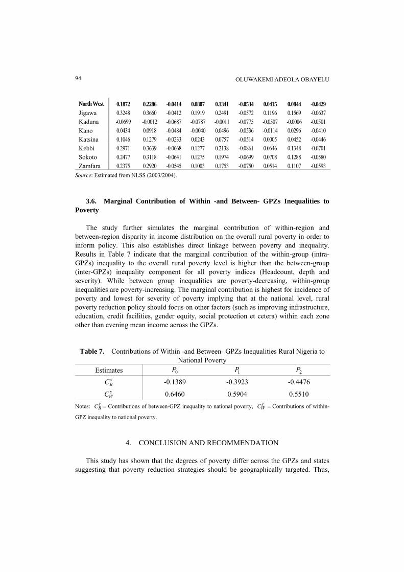
North West 0.1872 0.2286 -0.0414 0.0807 0.1341 -0.0534 0.0415 0.0844 -0.0429 Jigawa 0.3248 0.3660 -0.0412 0.1919 0.2491 -0.0572 0.1196 0.1569 -0.0637 Kaduna -0.0699 -0.0012 -0.0687 -0.0787 -0.0011 -0.0775 -0.0507 -0.0006 -0.0501 Kano 0.0434 0.0918 -0.0484 -0.0040 0.0496 -0.0536 -0.0114 0.0296 -0.0410 Katsina 0.1046 0.1279 -0.0233 0.0243 0.0757 -0.0514 0.0005 0.0452 -0.0446 Kebbi 0.2971 0.3639 -0.0668 0.1277 0.2138 -0.0861 0.0646 0.1348 -0.0701 Sokoto 0.2477 0.3118 -0.0641 0.1275 0.1974 -0.0699 0.0708 0.1288 -0.0580 Zamfara 0.2375 0.2920 -0.0545 0.1003 0.1753 -0.0750 0.0514 0.1107 -0.0593


3.6. Marginal Contribution of Within -and Between- GPZs Inequalities to

Poverty The study further simulates the marginal contribution of within-region and

between-region disparity in income distribution on the overall rural poverty in order to inform policy. This also establishes direct linkage between poverty and inequality. Results in Table 7 indicate that the marginal contribution of the within-group (intra- GPZs) inequality to the overall rural poverty level is higher than the between-group (inter-GPZs) inequality component for all poverty indices (Headcount, depth and severity). While between group inequalities are poverty-decreasing, within-group inequalities are poverty-increasing. The marginal contribution is highest for incidence of poverty and lowest for severity of poverty implying that at the national level, rural poverty reduction policy should focus on other factors (such as improving infrastructure, education, credit facilities, gender equity, social protection et cetera) within each zone other than evening mean income across the GPZs.

Table 7. Contributions of Within -and Between- GPZs Inequalities Rural Nigeria to National Poverty

Estimates 0P 1P 2P sBC -0.1389 -0.3923 -0.4476 sWC 0.6460 0.5904 0.5510

Notes: sBC Contributions of between-GPZ inequality to national poverty, s

WC Contributions of within-

GPZ inequality to national poverty.

4. CONCLUSION AND RECOMMENDATION This study has shown that the degrees of poverty differ across the GPZs and states

suggesting that poverty reduction strategies should be geographically targeted. Thus,


95

different poverty reduction interventions are needed to reduce poverty in the short-run across the different geopolitical zones. Where inequality is greater than mean income component, the policy should focus on inequality reduction (redistribution of income) through appropriate fiscal policies.

The study has four implications for policy measures aimed at alleviating rural poverty in Nigeria. First, there is a geographical dimension to the explanation of the variation of poverty rates across geopolitical zones. Policy measures with region-specific focus are thus advisable. For the coastal zone (South South), the significant influence of low standard of living calls for attention to the havoc that inflation may cause on the poor; for the northern GPZs, the emphasis should be placed on raising per capita expenditure; for the North Central zone, efforts to increase mean income should be supplemented by redistribution policy. Second, the GPZs are still quite heterogeneous, suggesting that geographical features such as distance to the sea, climate, topography of the terrain, and so on, are not the sole determinants of spatial inequality and poverty. Much of the similarity and dissimilarity among the GPZs can be traced to their industrial structures and the past and recent economic policies (Kanbur and Zhang, 2003).

Third, in GPZs and states where mean income level poses much problem to poverty alleviation, the efforts of the state and local government should focus on the formation of capital assets (human, social, financial and physical capitals). Finally, poverty alleviation strategies have an implication for national budget allocation and government expenditure for the whole country. This means that the share of Federal Government capital expenditure for poverty alleviation should be equitable across the GPZs and states.

REFERENCES

Adejuwon, J. (2008), “Vulnerability in Nigeria: A National-level Assessment,” in N. Leary, C. Conde, A. Nyong, and J. Pulhin, eds., Climate Change and Vulnerability, 198-217, London: Earthscan.

Adigun, G.T., and T.T. Awoyemi (2014), “Economic Growth, Income Redistribution and Poverty Reduction: Experiences from Rural Nigeria,” Asian Journal of Agricultural Extension, Economics & Sociology, 3(6), 638-653.

Agunwamba, A., D. Bloom, A. Friedman, M. Ozolins, L. Rosenberg, D. Steven, and M.Weston (2009), “Nigeria: The Next Generation - Literature Review,” funded by the British Council Nigeria, May.

Ajakaiye, D.O., and V.A. Adeyeye (2001), “The Nature of Poverty in Nigeria,” NISER Monograph Series, 13, Nigerian Institute of Social and Economic Research, Ibadan, Nigeria.

Araar, A. (2006), “On the Decomposition of the Gini Coefficient: An Exact Approach


with an Illustration using Cameroonian Data,” Centre Interuniversitaire sur le risqué, les politiques économiques et l’emploi Cahier de recherché Working Paper, 06-02.

Araar, A., and T.T. Awoyemi (2006), “Poverty and Inequality Nexus: Illustrations with Nigerian Data,” CIRPÉE Working Paper, 06-38, Available at https://depot.erudit. org/bitstream/001155dd/1/CIRPEE06-38.pdf.

Asadurian, T., E. Nnadozie, and L. Wantchekon (2006), “Transfer Dependence and Regional Disparities in Nigerian Federalism,” in J. Wallack, and T.N. Srinivasan, eds., Federalism and Economic Reform: International Perspectives, 407-455, Cambridge: Cambridge University Press.

Bourguignon, F. (2004), “The Poverty-Growth-Inequality Triangle,” presented at the Indian Council for Research on International Economic Relations, New Delhi on February 4, 2004.

Canagarajah, S., J. Ngwafon, and S. Thomas (1997), “The Evolution of Poverty and Welfare in Nigeria, 1985-92,” Policy Research Working Paper, 1715.

Datt, G., and M. Ravallion (1992), “Growth and Redistribution Components of Changes in Poverty Measures: A Decomposition with Application to Brazil and India in the 1980s,” Journal of Development Economics, 38, 275-295.

Dhongde, S. (2003), “Spatial Decomposition of Poverty in India,” prepared for the UNU/WIDER Project Conference on Spatial Inequality in Asia, United Nations University Centre, Tokyo, 28-29 March, 2003.

Duclos, J.-Y., and A. Araar (2006), “Poverty and Equity: Measurement, Policy and Estimation with DAD,” Springer and the International Development Research Centre (IDRC).

Foster, J., J. Greer, and E. Thorbecke (1984), “A Class of Decomposable Poverty Measures,” Econometrica, 52(3), 761-765.

Kakwani, N. (1993), “Poverty and Economic Growth with Application to Côte d’Ivoire,” Review of Income and Wealth, 39,121-139.

Kanbur, R., and X. Zhang (2003), “Fifty Years of Regional Inequality in China: A Journey Through Central Planning, Reform and Openness,” presented at the UNU-WIDER Conference on Spatial Inequality in Asia, Tokyo, 28-29 March, 2003.

Kolenikov, S., and A.F. Shorrocks (2003), “A Decomposition Analysis of Regional Poverty in Russia,” Discussion Paper, 74, Helsinki: WIDER.

Lawanson, A.O., and O. Olaniyan (2013), “Health Expenditure and Health Status in Northern and Southern Nigeria: A Comparative Analysis Using National Health Account Framework,” African Journal of Health Economics, 3, 1-13.

Molini, V. (2005), “The Transformation of the Vietnamese Earnings Distribution during the Transition: A Micro-Simulation Using Shapley’s Value,” SOW-VU Working Paper, Amsterdam.

Minot, N., B. Baulch, and M. Epprecht (2003), “Poverty and Inequality in Vietnam: Spatial Patterns and Geographic Determinants,” A Report of International Food Policy Research Institute and Institute of Development Studies.


97

NBS (2005), Poverty Profile for Nigeria, National Bureau of Statistic, Abuja Ganfeek Ventures.

NSSL (2003/2004), Nigeria - Nigeria Living Standard Survey 2003/2004, First round, Published by the National Bureau of Statistics, NGA-NBS-NLSS-2003-v1.2.

Ogwumike, F.O., and M.K. Akinnibosun (2013), “Determinants of Poverty Among Farming Households in Nigeria,” Mediterranean Journal of Social Sciences, 4(2), 365-373.

Olaniyan, O. (2002), “The Effects of Household Endowments on Poverty in Nigeria,” African Journal of Economic Policy, 9(2), 77-102 .

Omonona, B.T. (2010), “Quantitative Analysis of Rural Poverty in Nigeria,” International Food Policy Research Institute (IFPRI), Nigeria Strategy Support Program (NSSP), Policy Brief , 17.

Osinubi, T.S. (2003), “Macroeconomic Policies and Pro-Poor Growth in Nigeria,” Conference on Inequality, Poverty and Human-Well Being, World Institute for Development Economics Research (WIDER), Helsinki, Finland, 30-31th May, 2003.

Oyekale, O.S., A.I. Adeoti, and T.O. Oyekale (2006), “Measurement and Sources of Income Inequality among Rural and Urban Households in Nigeria (December 2006),” PMMA Working Paper, 2006-20, Final Report submitted to Poverty and Economic Policy Network (PEP), Universite Laval, Canada.

Shaw, W. (1996), The Geography of United States Poverty, New York: Garland Publishing.

Uneze, E., and A. Adeniran (2014), “Explaining the Spatial and Sectoral Variations in Growth Pro-poorness in Nigeria,” prepared for the IARIW 33rd General Conference Rotterdam, the Netherlands, August 24-30, 2014.

World Bank (1996), “Nigeria: Poverty in the Midst of Plenty - The Challenge of Growth with Inclusion,” UNI Report, 14733, Washington, D.C. (May).

Zhang, Y., and G. Wan (2005), “Why Do Poverty Rates Differ from Region to Region? The Case of Urban China,” UNU-WIDER Research Paper, 2005/56, Helsinki.

Mailing Address: Oluwakemi Adeola Obayelu, Department of Agricultural Economics, University of Ibadan, Nigeria. E-mail: [email protected].

Received May 8, 2014, Revised August 20, 2014, Accepted October 10, 2014.

Documents

SPATIAL DECOMPOSITION OF POVERTY IN RURAL …jed.or.kr/full-text/39-4/4.pdf · SPATIAL DECOMPOSITION OF POVERTY IN RURAL NIGERIA 79 Geographically-based theories of poverty calls