Embed Size (px)
Citation preview

Spatial and Social Inequalities in Human Development: India in the Global Context
By Amitabh Kundu, P.C. Mohanan and K. Varghese

1
Disclaimer The views in the publication are those of the authors’ and do not necessarily reflect those of the United Nations Development Programme Copyright © UNDP 2013. All rights reserved. Published in India. Cover Photo © UNDP India

2
Spatial and Social Inequalities in Human Development: India in the Global Context
Amitabh Kundu, P. C. Mohanan and K. Varghese 1. Introduction The vision of India emerging as a Giant in the global economic scene seems to dominate the contemporary discussion on its growth performance, leading to coinage of phrases like “amazing India” and metamorphosis of a “slumbering elephant” etc. The development scenario is viewed optimistically in the global context not only in terms of the pace of its growth but also because of its capacity to stand out in periods of global economic crisis. The country’s seven and a half per cent growth performance during the Tenth and Eleventh Plan period against the projected scenario of 9 per cent growth, particularly its deceleration in 2011-12, has not dented this optimism. In the context of growth in employment, too, the economy has done reasonably well, allaying fears of jobless growth, the key concern in the late 1990s. There seems to be, however, a shared concern that the country has not been successful in transforming “its growth into development”, the problem manifesting most significantly in serious regional imbalances, rural urban disparities and inequalities across social and religious groups. It would be important to probe into these questions. The present paper begins with a global overview, analyzing the pattern of the loss in human development in different countries, when computing the inequality adjusted indices, as proposed by UNDP (2010), by grouping the countries into three development categories. A similar analysis is attempted by taking all the states of India as the units of analysis. This is done in the second section which follows the present introductory section. The next section looks at the trend of inequalities in socio-economic indicators, primarily in terms of per capita State Domestic Product, consumption expenditure and indicators pertaining to education, health and access to civic amenities, based on the latest statistics at state level collected from national sources. Inequality across socio-religious groups and gender have been analysed in the fourth section. The final section gives a summary of findings and provides a perspective for its future development in the context of inequities in the socio-economic system.
2. Inequality in Dimensions of Human Development in Global Context
A major anxiety in the context of the targets set through Millennium Development Goals (MDGs) to be achieved by 2015 is that there will be significant deficits in achievement and these will be particularly high in the developing countries, including the emerging economies. The deficits are likely to be high in terms of health and education linked indicators, which can be attributed to the inequalities in availability and access to the related facilities across states, regions, cities as also across social and religious groups. These, at the second level can be attributed to the inequality in access to basic services, particularly, safe drinking water and sanitation.
3
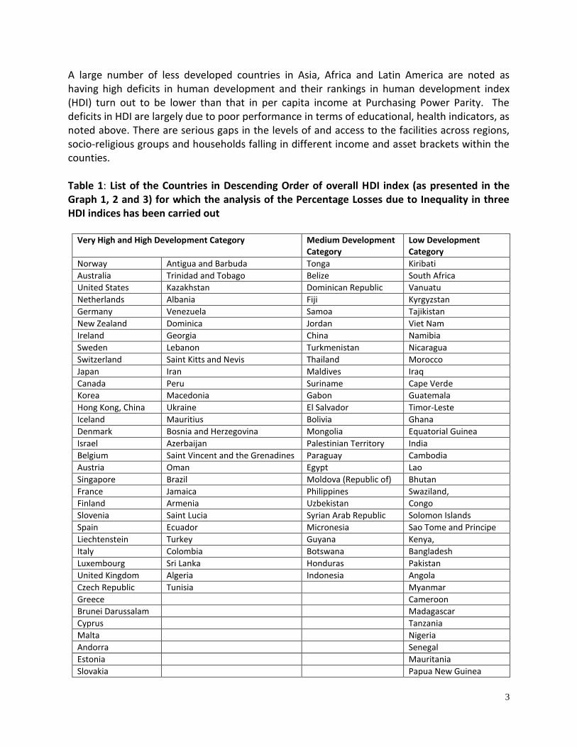
A large number of less developed countries in Asia, Africa and Latin America are noted as having high deficits in human development and their rankings in human development index (HDI) turn out to be lower than that in per capita income at Purchasing Power Parity. The deficits in HDI are largely due to poor performance in terms of educational, health indicators, as noted above. There are serious gaps in the levels of and access to the facilities across regions, socio-religious groups and households falling in different income and asset brackets within the counties. Table 1: List of the Countries in Descending Order of overall HDI index (as presented in the Graph 1, 2 and 3) for which the analysis of the Percentage Losses due to Inequality in three HDI indices has been carried out
Very High and High Development Category Medium Development Category
Low Development Category
Norway Antigua and Barbuda Tonga Kiribati
Australia Trinidad and Tobago Belize South Africa
United States Kazakhstan Dominican Republic Vanuatu
Netherlands Albania Fiji Kyrgyzstan
Germany Venezuela Samoa Tajikistan
New Zealand Dominica Jordan Viet Nam
Ireland Georgia China Namibia
Sweden Lebanon Turkmenistan Nicaragua
Switzerland Saint Kitts and Nevis Thailand Morocco
Japan Iran Maldives Iraq
Canada Peru Suriname Cape Verde
Korea Macedonia Gabon Guatemala
Hong Kong, China Ukraine El Salvador Timor-Leste
Iceland Mauritius Bolivia Ghana
Denmark Bosnia and Herzegovina Mongolia Equatorial Guinea
Israel Azerbaijan Palestinian Territory India
Belgium Saint Vincent and the Grenadines Paraguay Cambodia
Austria Oman Egypt Lao
Singapore Brazil Moldova (Republic of) Bhutan
France Jamaica Philippines Swaziland,
Finland Armenia Uzbekistan Congo
Slovenia Saint Lucia Syrian Arab Republic Solomon Islands
Spain Ecuador Micronesia Sao Tome and Principe
Liechtenstein Turkey Guyana Kenya,
Italy Colombia Botswana Bangladesh
Luxembourg Sri Lanka Honduras Pakistan
United Kingdom Algeria Indonesia Angola
Czech Republic Tunisia Myanmar
Greece Cameroon
Brunei Darussalam Madagascar
Cyprus Tanzania
Malta Nigeria
Andorra Senegal
Estonia Mauritania
Slovakia Papua New Guinea
4
Qatar Nepal
Hungary Lesotho
Barbados Togo
Poland Yemen
Chile Haiti
Lithuania Uganda
United Arab Emirates
Zambia
Portugal Djibouti
Latvia Gambia
Argentina Benin
Seychelles Rwanda
Croatia Côte d'Ivoire
Bahrain Comoros
Bahamas Malawi
Belarus Sudan
Uruguay Zimbabwe
Montenegro Ethiopia
Palau Liberia
Kuwait Afghanistan
Russian Federation Guinea-Bissau
Romania Sierra Leone
Bulgaria Burundi
Saudi Arabia Guinea
Cuba Central African Republic
Panama Eritrea
Mexico Mali
Costa Rica Burkina Faso
Grenada Chad
Libya Mozambique
Malaysia Congo
Serbia Niger
UNDP (2010) has proposed a procedure for computation of the loss in the three dimensions of human development - income, education and health, based on the gap between the original index and inequality adjusted index, taken as a percentage of the original index. The figures for the loss for all the countries for the year 2013, taken from UNDP (2013), have been analysed in the section. The countries have been placed in three categories of human development, as shown in Table 1. Graph 1 depicts the loss in these dimensions of income, health and education due to inequality, taking into consideration 94 countries in very high and high development category, arranged in a descending order. A few countries in each category unfortunately report no information, and consequently there are gaps in the graph. It may be noted that the loss in income index, due to intra country inequality, is very high compared to indices for other dimensions, as assessed from the high average value of the loss. So is the variation in the loss across the countries, measured through standard deviation (Table 2). In case of the loss in education index, the average value is low and so is its variation. Furthermore, the loss in health index is the least and so is the inter-country variation. This implies that the developed countries, despite their high income inequality within the countries and significant differences
5
across them, are able, in general, to ensure fairly good health conditions and equal access to education for all sections of their population.

6
Table 2: Percentage Loss in Three Human Development Indices Due to Inequality Adjustment - 2013
Category of Countries Life expectancy Education Income
Average
Developed 8.1 9.1 20.1
Medium developed 16.5 21.1 26.8
Least developed 32.9 34.6 28.8
India 33.20 41.22 13.96
Standard Deviation
Developed 4.1 7.2 9.5
Medium developed 5.4 11.6 8.7
Least developed 10.2 10.5 11.3
India 7.99 5.43 2.56 Note: Compiled from UNDP (2013) and Suryanarayana et. al. (2011)
Graph 1: Loss in the inequality adjusted indices of human development for the countries in very high and high development category, in descending order of overall HDI, 2013
0.0
5.0
10.0
15.0
20.0
25.0
30.0
35.0
40.0
45.0
50.0
No
rway
Ger
man
y
Swit
zerl
and
Ho
ng
Ko
ng,
Ch
ina
(SA
R)
Be
lgiu
m
Fin
lan
d
Ital
y
Gre
ece
An
do
rra
Hu
nga
ry
Lith
uan
ia
Arg
en
tin
a
Bah
amas
Pal
au
Bu
lgar
ia
Me
xico
Mal
aysi
a
Kaz
akh
stan
Geo
rgia
Pe
ru
Bo
snia
an
d H
erze
govi
na
Bra
zil
Ecu
ado
r
Alg
eria
Loss (%) LExp
Loss (%) Edu
Loss (%) Income
7
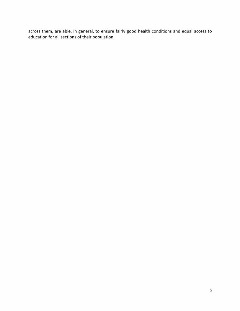
Unfortunately, the situation changes when we consider the 27 countries in the middle category of human development (Graph 2). The average loss in income index due to intra-country inequality goes up by 56 per cent compared to the very high and high development category but that in health and education, the indices go up by 124 per cent and 200 per cent respectively. The inter country variations are also higher here, as may be seen in the higher value of standard deviation. In case of the third category of 65 less developed countries, the average loss due to income inequality is very high but less than that in the medium category. However, the losses due to health and educational inequality in absolute and relative terms are extremely high, much above that of other two categories (Graph 3). Most significantly, the inter country inequality in health index in these countries is more than two times that of the countries belonging to higher categories of human development. Graph 2: Loss in the inequality adjusted indices of human development for the countries in medium development category, in descending order of overall HDI, 2013
0.0
5.0
10.0
15.0
20.0
25.0
30.0
35.0
40.0
45.0
50.0
Ton
ga
Do
min
ican
Rep
ub
lic
Sam
oa
Ch
ina
Thai
lan
d
Suri
nam
e
El S
alva
do
r
Mo
ngo
lia
Par
agu
ay
Mo
ldo
va (
Rep
ub
lic o
f)
Uzb
eki
stan
Mic
ron
esi
a (F
ede
rate
d S
tate
s o
f)
Bo
tsw
ana
Ind
on
esi
a
Loss (%) LExp
Loss (%) Edu
Loss (%) Income
8
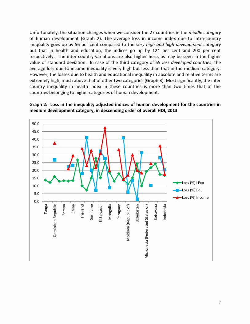
Graph 3: Loss in the inequality adjusted indices of human development for the countries in low development category, in descending order of overall HDI, 2013
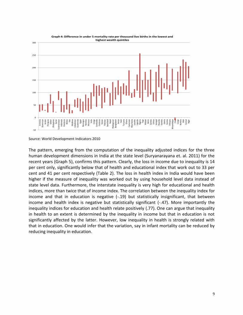
The loss in health index can partly be attributed to inequality in access to water and sanitation, particularly in urban areas. The analysis of cross country data show that the health outcome in a country depends not so much on average health expenditure but on marginal expenditure on water and sanitation in marginal areas within their cities1. The differences in the under 5 mortality rate between the households in the highest and the lowest quintiles are presented for different countries in Graph 4 that sharply bring out the inequality in one of the major indicators of health outcome.
1 See Cheng, Schuster-Wallace, Watt, Newbold and Mente (2012)
0.0
10.0
20.0
30.0
40.0
50.0
60.0
70.0
80.0
Kir
ibat
i
Kyr
gyzs
tan
Nam
ibia
Iraq
Tim
or-
Lest
e
Ind
ia
Bh
uta
n
Solo
mo
n Is
lan
ds
Ban
glad
esh
Mya
nm
ar
Tan
zan
ia (
Un
ite
d R
epu
blic
of)
Mau
rita
nia
Leso
tho
Hai
ti
Djib
ou
ti
Rw
and
a
Mal
awi
Eth
iop
ia
Gu
ine
a-B
issa
u
Gu
ine
a
Mal
i
Mo
zam
biq
ue
Loss (%) LExp
Loss (%) Edu
Loss (%) Income
9
-50
0
50
100
150
200
250
300
Arm
enia
Dom
inic
anJo
rdan
Para
guay
Gab
onPh
ilipp
ines
Syria
nTu
rkm
enist
anIn
done
siaH
ondu
ras
Boliv
iaVi
etM
oldo
vaU
zbek
ista
nG
uate
mal
aEg
ypt
Nic
arag
uaN
amib
iaM
oroc
coIn
dia
Cong
oCa
mbo
dia
Com
oros
Yem
enPa
kist
anSw
azila
ndN
epal
Mad
agas
car
Bang
lade
shKe
nya
Hai
tiTa
nzan
iaG
hana
Cam
eroo
nM
aurit
ania
Leso
tho
Uga
nda
Nig
eria
Togo
Mal
awi
Beni
nZa
mbi
aEr
itrea
Sene
gal
Rwan
daG
ambi
aLi
beria
Gui
nea
Ethi
opia
Moz
ambi
que
Chad
Cong
oBu
rkin
aM
ali
Cent
ral
Nig
er
Graph 4: Difference in under 5 mortality rate per thousand live births in the lowest and highest wealth quintiles
Source: World Development Indicators 2010
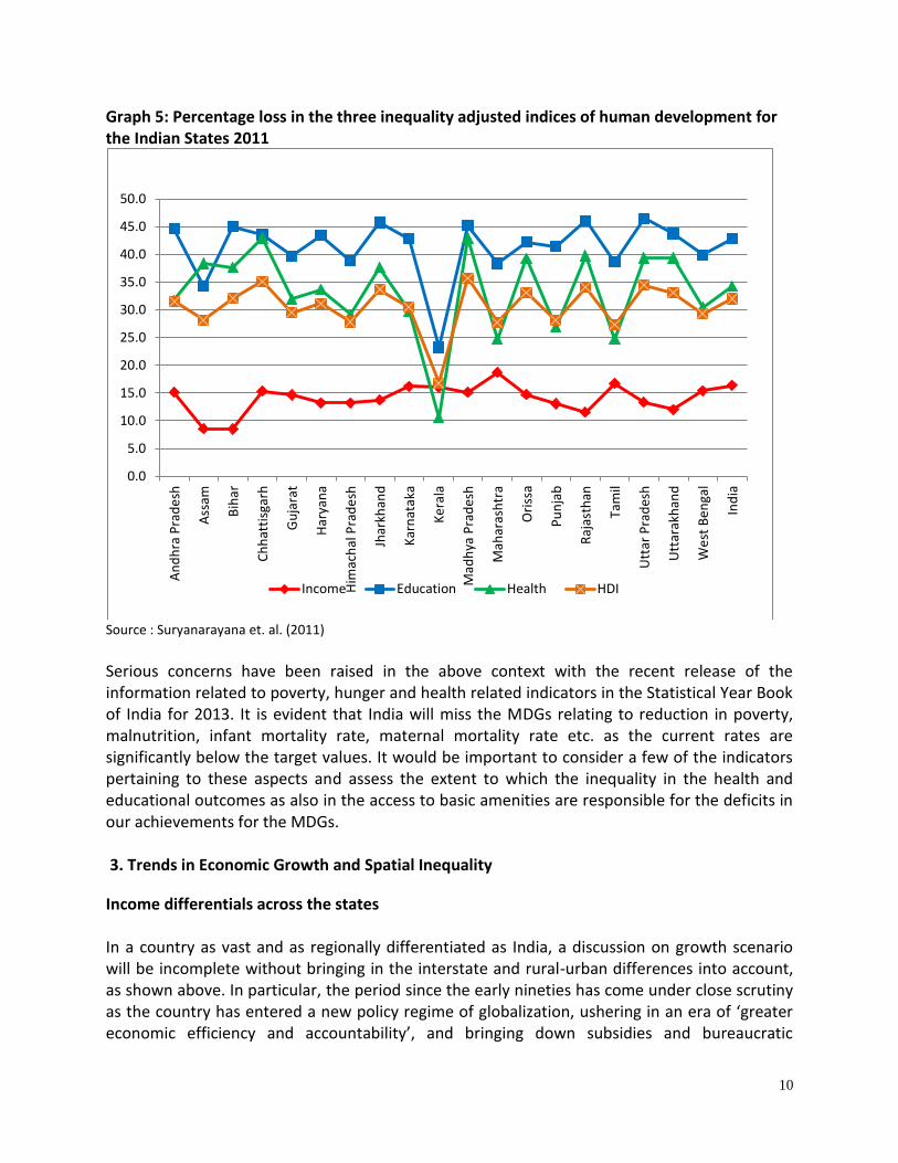
The pattern, emerging from the computation of the inequality adjusted indices for the three human development dimensions in India at the state level (Suryanarayana et. al. 2011) for the recent years (Graph 5), confirms this pattern. Clearly, the loss in income due to inequality is 14 per cent only, significantly below that of health and educational index that work out to 33 per cent and 41 per cent respectively (Table 2). The loss in health index in India would have been higher if the measure of inequality was worked out by using household level data instead of state level data. Furthermore, the interstate inequality is very high for educational and health indices, more than twice that of income index. The correlation between the inequality index for income and that in education is negative (-.19) but statistically insignificant, that between income and health index is negative but statistically significant (-.47). More importantly the inequality indices for education and health relate positively (.77). One can argue that inequality in health to an extent is determined by the inequality in income but that in education is not significantly affected by the latter. However, low inequality in health is strongly related with that in education. One would infer that the variation, say in infant mortality can be reduced by reducing inequality in education.
10
Graph 5: Percentage loss in the three inequality adjusted indices of human development for the Indian States 2011
Source : Suryanarayana et. al. (2011)
Serious concerns have been raised in the above context with the recent release of the information related to poverty, hunger and health related indicators in the Statistical Year Book of India for 2013. It is evident that India will miss the MDGs relating to reduction in poverty, malnutrition, infant mortality rate, maternal mortality rate etc. as the current rates are significantly below the target values. It would be important to consider a few of the indicators pertaining to these aspects and assess the extent to which the inequality in the health and educational outcomes as also in the access to basic amenities are responsible for the deficits in our achievements for the MDGs. 3. Trends in Economic Growth and Spatial Inequality
Income differentials across the states In a country as vast and as regionally differentiated as India, a discussion on growth scenario will be incomplete without bringing in the interstate and rural-urban differences into account, as shown above. In particular, the period since the early nineties has come under close scrutiny as the country has entered a new policy regime of globalization, ushering in an era of ‘greater economic efficiency and accountability’, and bringing down subsidies and bureaucratic
0.0
5.0
10.0
15.0
20.0
25.0
30.0
35.0
40.0
45.0
50.0
An
dh
ra P
rad
esh
Ass
am
Bih
ar
Ch
hat
tisg
arh
Gu
jara
t
Har
yan
a
Him
ach
al P
rad
esh
Jhar
khan
d
Kar
nat
aka
Ke
rala
Mad
hya
Pra
des
h
Mah
aras
htr
a
Ori
ssa
Pu
nja
b
Raj
asth
an
Tam
il
Utt
ar P
rad
esh
Utt
arak
han
d
We
st B
en
gal
Ind
ia
Income Education Health HDI
11
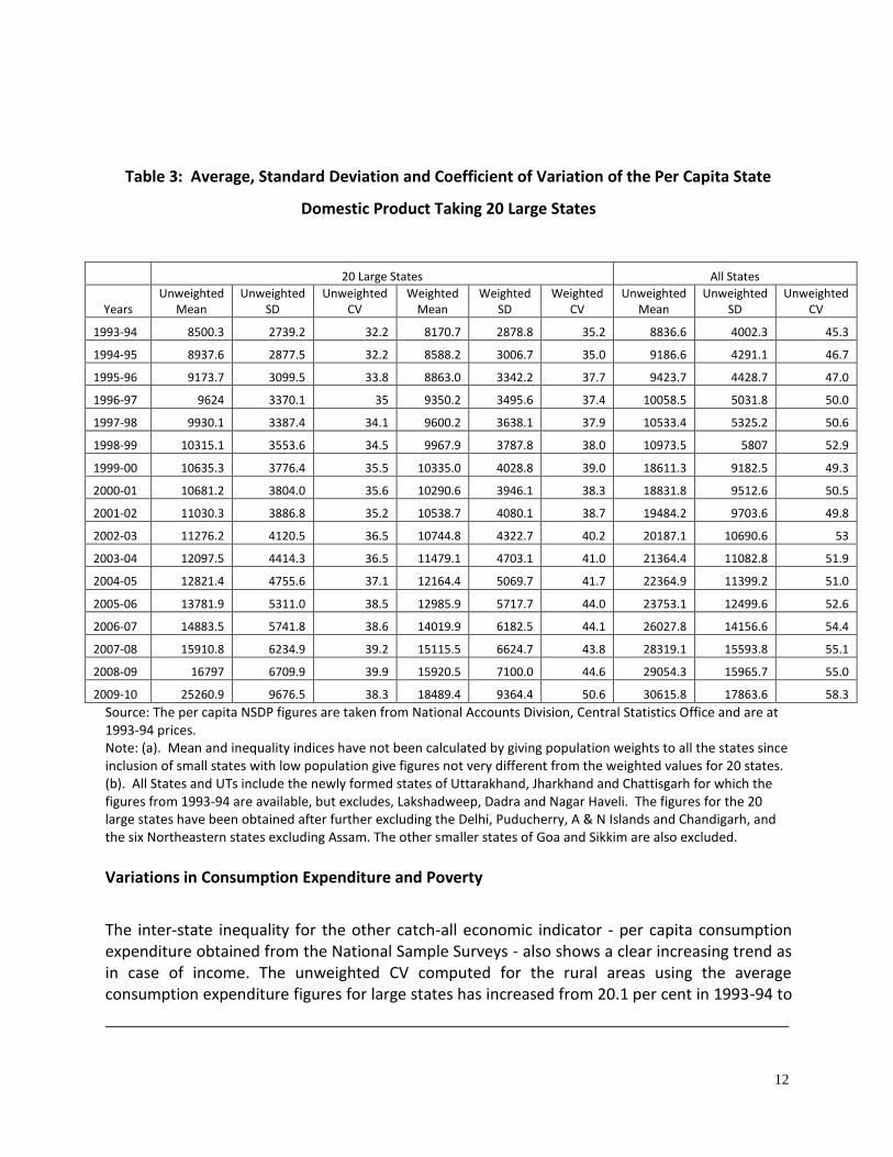
controls2 that were supposed to ensure regional balance in development. In view of that, income inequality measures have been computed for the years from 1993-94 to 2009-10, for which the data are available, using the per capita state domestic product figures at constant prices. The data up to the year 2004-05 obtained from CSO are taking the 1993-94 as the base year while for the subsequent years they are with 1999-00 base year. However, the figures for coefficient of variation and Gini coefficient, that are relative measures of inequality, are unlikely to be affected by this as these are based on a uniform methodology followed by all States. Unweighted coefficients of variation have been worked out by giving equal weights to each state while the weighted values have been worked out by assigning weights equal to their population.
It is important to note that inequality across the states, measured through a standard measure of relative deviation like coefficient of variation in the per capita SDP, has gone up in the country over the entire period since 1993-94. The increase in inequality is noted both when we consider only 20 larger states or all the states in the country. There is, thus, no evidence to suggest that measures of globalization have brought down regional imbalance. The trend of growing regional inequity has continued, possibly at a slightly higher pace after 2003-04 when the overall growth in GDP for the country shot up to 8 per cent per annum and many of the backward states, including those in North East, exhibited even higher growth rates. It is only during 2007-09 that the interstate disparity in the growth rate of SDP records a stability or decline which is reflected in a slower increase in CV in per capita SDP. Unfortunately, this growth process has not been sustained in many of the backward states which has led to income inequality increasing again in recent years.
Importantly, weighted CV is higher than the unweighted CV in all the years. This is because the relatively more populous states like Bihar and Uttar Pradesh report per capita SDP significantly below the national average. Furthermore, the rise in the weighted CV is higher than the unweighted CV since the more populous states have not improved their per capita income levels as much as the less populated states.
Several other studies analyzing the trend in inequality in per capita income, based on coefficient of variation (CV) and Gini-coefficient confirm the thesis of accentuation of regional imbalance3. Studies show that the low income states like Bihar, Chhattisgarh, Jharkhand, Orissa, and Uttar Pradesh and Uttarakhand and Madhya Pradesh had reported low economic growth during eighties. In most cases their average growth rates have gone down further during the nineties which is reflected in increase in the CV, as discussed above. The less developed states have the disadvantage not only of a low growth rate but also high fluctuation in the rate from year to year4. What compounds their problems is that there is only a marginal decline in their population growth that have stayed much above the national average.
2 Ahluwalia (2000)
3 Ahmad et. al. (2008) and Planning Commission (2005) 4 Another important fact is that these states have reported a decline in per capita income or no growth in at least two years during
nineties, a problem not encountered in the middle or high income states.
12
Table 3: Average, Standard Deviation and Coefficient of Variation of the Per Capita State
Domestic Product Taking 20 Large States
20 Large States All States
Years Unweighted
Mean Unweighted
SD Unweighted
CV Weighted
Mean Weighted
SD Weighted
CV Unweighted
Mean Unweighted
SD Unweighted
CV
1993-94 8500.3 2739.2 32.2 8170.7 2878.8 35.2 8836.6 4002.3 45.3
1994-95 8937.6 2877.5 32.2 8588.2 3006.7 35.0 9186.6 4291.1 46.7
1995-96 9173.7 3099.5 33.8 8863.0 3342.2 37.7 9423.7 4428.7 47.0
1996-97 9624 3370.1 35 9350.2 3495.6 37.4 10058.5 5031.8 50.0
1997-98 9930.1 3387.4 34.1 9600.2 3638.1 37.9 10533.4 5325.2 50.6
1998-99 10315.1 3553.6 34.5 9967.9 3787.8 38.0 10973.5 5807 52.9
1999-00 10635.3 3776.4 35.5 10335.0 4028.8 39.0 18611.3 9182.5 49.3
2000-01 10681.2 3804.0 35.6 10290.6 3946.1 38.3 18831.8 9512.6 50.5
2001-02 11030.3 3886.8 35.2 10538.7 4080.1 38.7 19484.2 9703.6 49.8
2002-03 11276.2 4120.5 36.5 10744.8 4322.7 40.2 20187.1 10690.6 53
2003-04 12097.5 4414.3 36.5 11479.1 4703.1 41.0 21364.4 11082.8 51.9
2004-05 12821.4 4755.6 37.1 12164.4 5069.7 41.7 22364.9 11399.2 51.0
2005-06 13781.9 5311.0 38.5 12985.9 5717.7 44.0 23753.1 12499.6 52.6
2006-07 14883.5 5741.8 38.6 14019.9 6182.5 44.1 26027.8 14156.6 54.4
2007-08 15910.8 6234.9 39.2 15115.5 6624.7 43.8 28319.1 15593.8 55.1
2008-09 16797 6709.9 39.9 15920.5 7100.0 44.6 29054.3 15965.7 55.0
2009-10 25260.9 9676.5 38.3 18489.4 9364.4 50.6 30615.8 17863.6 58.3
Source: The per capita NSDP figures are taken from National Accounts Division, Central Statistics Office and are at 1993-94 prices. Note: (a). Mean and inequality indices have not been calculated by giving population weights to all the states since inclusion of small states with low population give figures not very different from the weighted values for 20 states. (b). All States and UTs include the newly formed states of Uttarakhand, Jharkhand and Chattisgarh for which the figures from 1993-94 are available, but excludes, Lakshadweep, Dadra and Nagar Haveli. The figures for the 20 large states have been obtained after further excluding the Delhi, Puducherry, A & N Islands and Chandigarh, and the six Northeastern states excluding Assam. The other smaller states of Goa and Sikkim are also excluded.
Variations in Consumption Expenditure and Poverty
The inter-state inequality for the other catch-all economic indicator - per capita consumption expenditure obtained from the National Sample Surveys - also shows a clear increasing trend as in case of income. The unweighted CV computed for the rural areas using the average consumption expenditure figures for large states has increased from 20.1 per cent in 1993-94 to

13
28.2 per cent in 2004-05 and then to 31.0 per cent in 2009-10 (Graph 6). This increasing pattern can be observed when we consider the figures for million plus cities and other smaller urban centres as well, taking the states as units of observation and computing the CV from unit level data. The inter-state inequality in case of metro cities initially works out to be low but exhibits a sharp rise. It goes up from 12.2 per cent in 1993-94 to 21.9 per cent in 2009-10. One would infer that the cities were similar in terms of their average expenditure levels in early nineties but have become more disparate over time. This is because many of them subsequently have got linked to global market and experienced high income growth. The non- metropolitan urban centres, on the other hand, exhibited interstate inequality similar to that of rural areas and this has not gone up over the two decades. This is largely because of stagnation of their economies and absence of sectoral diversification.
The calculation of CV for the years 2004-05 and 2009-10 in Graph 6 is based on the average figure for per capita consumption expenditure for 20 large states (see Notes under Table 3), built through unit level data. The CV for 1993-94, is also based on the average expenditure figures computed from unit level data but for 17 states. The number is reduced here as Bihar stands for the undivided state comprising Bihar and Jharkhand while Madhya Pradesh includes Chhattisgarh and Uttar Pradesh includes Uttarakhand. Graph 7, however, gives the CVs obtained directly from the unit (household) level data without first computing the per capita expenditure figures at the state level and then computing the CV and consequently is much higher than those of Graph 6. This further shows that inequality in urban areas is much higher than rural areas in 2009-10. Also, the increase in inequality has been very sharp in urban areas, particularly in metro cities, during 1993-2009. The most significant point is that inequality in the metro cities was very low in early nineties but has gone up sharply in the recent past. Not only that the metro cities differ from one another across the states but also that there is much higher inequality within the cities now than before two decades, as one would infer from rising value of CV in Graph 7.

14
Graph 6: Coefficients of Variation of monthly per capita expenditure across States
Source: Computed from NSS unit level data
20
.1
12
.2
20
.0
19
.0
18
.2
28
.2
17
.6
19
.2
16
.6
25
.2
31
.0
21
.9
23
.8
21
.7
28
.2
0.0
5.0
10.0
15.0
20.0
25.0
30.0
35.0
Rural Cities withMillion Plus
Pop
Other UrbanAreas
All Urban Total
1993-94
2004-05
2009-10
15
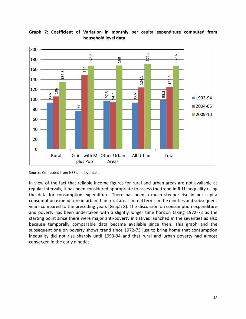
Graph 7: Coefficient of Variation in monthly per capita expenditure computed from household level data
Source: Computed from NSS unit level data.
In view of the fact that reliable income figures for rural and urban areas are not available at regular intervals, it has been considered appropriate to assess the trend in R-U inequality using the data for consumption expenditure. There has been a much steeper rise in per capita consumption expenditure in urban than rural areas in real terms in the nineties and subsequent years compared to the preceding years (Graph 8). The discussion on consumption expenditure and poverty has been undertaken with a slightly longer time horizon taking 1972-73 as the starting point since there were major anti-poverty initiatives launched in the seventies as also because temporally comparable data became available since then. This graph and the subsequent one on poverty shows trend since 1972-73 just to bring home that consumption inequality did not rise sharply until 1993-94 and that rural and urban poverty had almost converged in the early nineties.
93
.6
77
97
.5
93
.6
98
.3
10
6
14
9
94
.2
12
4.1
12
4.9
13
4.8
16
7.7
16
8
17
1.4
16
7.6
0
20
40
60
80
100
120
140
160
180
200
Rural Cities with Mplus Pop
Other UrbanAreas
All Urban Total
1993-94
2004-05
2009-10
16
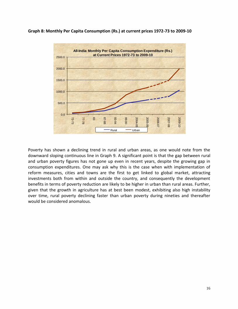
Graph 8: Monthly Per Capita Consumption (Rs.) at current prices 1972-73 to 2009-10
0.0
500.0
1000.0
1500.0
2000.0
2500.0
72-7
3
77-7
8
83
87-8
8
93-9
4
99-0
0
2004-0
5
2005-0
6
2006-0
7
2007-0
8
2009-1
0
All-India Monthly Per Capita Consumption Expenditure (Rs.)
at Current Prices 1972-73 to 2009-10
Rural Urban
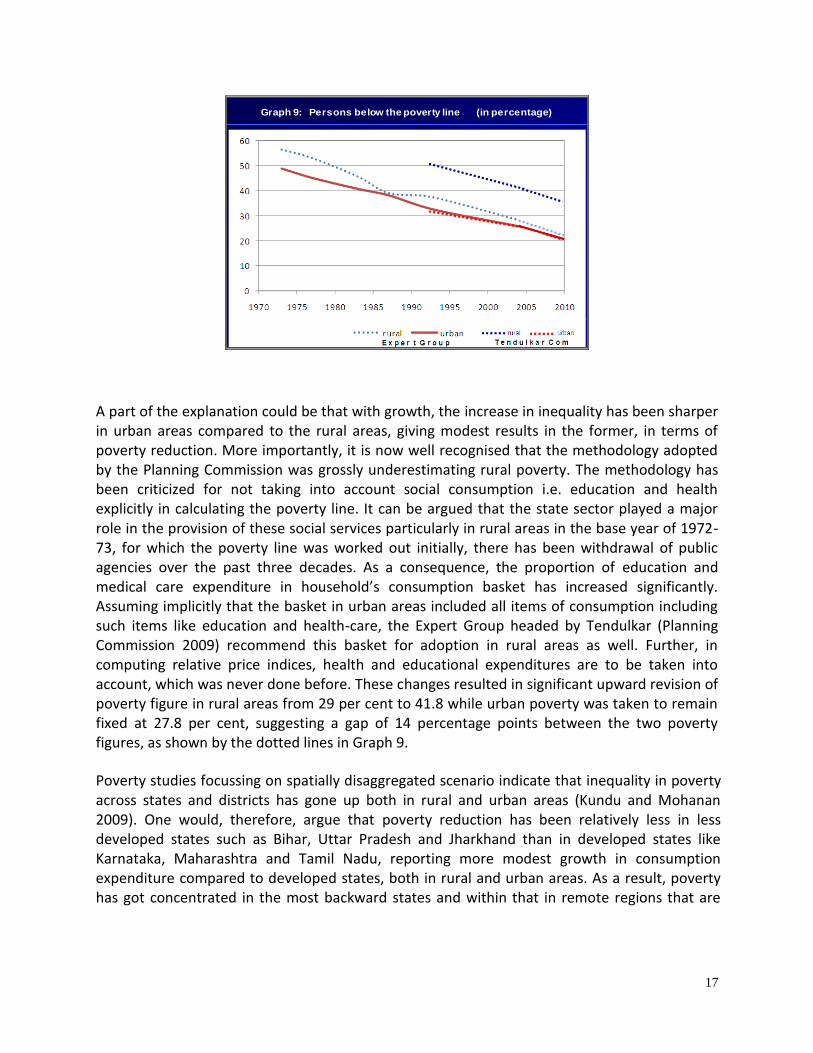
Poverty has shown a declining trend in rural and urban areas, as one would note from the downward sloping continuous line in Graph 9. A significant point is that the gap between rural and urban poverty figures has not gone up even in recent years, despite the growing gap in consumption expenditures. One may ask why this is the case when with implementation of reform measures, cities and towns are the first to get linked to global market, attracting investments both from within and outside the country, and consequently the development benefits in terms of poverty reduction are likely to be higher in urban than rural areas. Further, given that the growth in agriculture has at best been modest, exhibiting also high instability over time, rural poverty declining faster than urban poverty during nineties and thereafter would be considered anomalous.
17
Graph 9: Persons below the poverty line (in percentage)
A part of the explanation could be that with growth, the increase in inequality has been sharper in urban areas compared to the rural areas, giving modest results in the former, in terms of poverty reduction. More importantly, it is now well recognised that the methodology adopted by the Planning Commission was grossly underestimating rural poverty. The methodology has been criticized for not taking into account social consumption i.e. education and health explicitly in calculating the poverty line. It can be argued that the state sector played a major role in the provision of these social services particularly in rural areas in the base year of 1972-73, for which the poverty line was worked out initially, there has been withdrawal of public agencies over the past three decades. As a consequence, the proportion of education and medical care expenditure in household’s consumption basket has increased significantly. Assuming implicitly that the basket in urban areas included all items of consumption including such items like education and health-care, the Expert Group headed by Tendulkar (Planning Commission 2009) recommend this basket for adoption in rural areas as well. Further, in computing relative price indices, health and educational expenditures are to be taken into account, which was never done before. These changes resulted in significant upward revision of poverty figure in rural areas from 29 per cent to 41.8 while urban poverty was taken to remain fixed at 27.8 per cent, suggesting a gap of 14 percentage points between the two poverty figures, as shown by the dotted lines in Graph 9.
Poverty studies focussing on spatially disaggregated scenario indicate that inequality in poverty across states and districts has gone up both in rural and urban areas (Kundu and Mohanan 2009). One would, therefore, argue that poverty reduction has been relatively less in less developed states such as Bihar, Uttar Pradesh and Jharkhand than in developed states like Karnataka, Maharashtra and Tamil Nadu, reporting more modest growth in consumption expenditure compared to developed states, both in rural and urban areas. As a result, poverty has got concentrated in the most backward states and within that in remote regions that are
18
more difficult to access, both for market forces and governmental programmes5. Understandably, the elasticity of poverty reduction to income growth has been less in the Eleventh Plan compared to that of earlier plans.
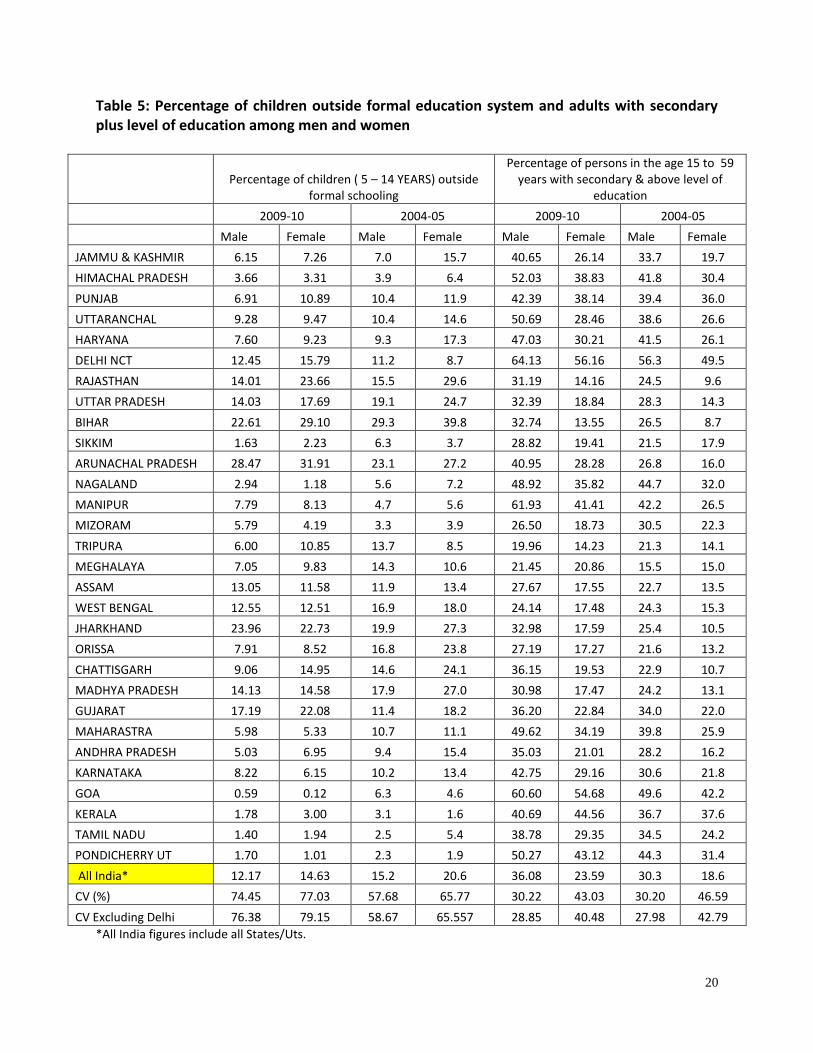
Education and Health In analyzing the inequality in the levels of educational development across the states, it would be important to compute indicators of educational attainments with reference to specific age groups. This is because including the people in higher age groups would mean carrying forward inequity of the earlier generation in evaluating current developmental efforts. Consequently, the indicators pertaining to children in the school going age group, their current attendance have been considered appropriate for the study. Also, since the capacity to earn income substantially depends on the educational attainments of the working, education level of persons in the prime working age group - 25 to 59 years - has been considered for each social group. The percentages of children outside the formal education system (Table 4 & 5), despite a decline in recent years, work out as very high in 2009-10 for boys and girls and in both in rural and urban areas, suggesting that there will be significant deficit in attaining the MDG goals of universal primary education and eliminating gender disparity in all levels of education by 2015. Importantly, the RU disparity in this indicator is not very high compared to that in the percentage of persons with secondary and higher education. The latter in urban areas is two and a half times that in rural areas. The low educational attainment in 15-59 age group in rural areas reflects the cumulative impact of deprivation in earlier years. By both the indicators, one would, however, argue that the situation has improved during 2005-10. What, however, is disturbing that the inequality in both the indicators across the states has gone up in both urban and rural areas. A similar picture is noted in case of the indicators for males and females in 15-59 age group across the states (Table 5). The situation has improved for both and there is indication that gender disparity has gone down in recent years. This may be inferred from the female male ratio in the percentage of children outside the formal system declining from 1.35 to 1.20. Furthermore, the male educational attainment was 63 per cent higher than that of women in 2001, the figure going down to 53 per cent only in 2011. In case for interstate inequality, however, the trend is the opposite. For men the inequality has gone up distinctly in both the indicators while for women, it has gone up in case of children outside the formal education system. For educational attainment, the inequality seems to have remained stable during 2001-11.
5 Sivaramakrishnan, Kundu and Singh (2005)

19
Table 4: Percentage of children outside formal education system and adults with secondary plus level of education in rural and urban areas
Percentage of children ( 5 – 14 YEARS)
outside formal schooling
Percentage of persons in the age 15 to 59 years with secondary & above level of
education
States/UTs/NCT 2009-10 2004-05 2009-10 2004-05
RURAL URBAN RURAL URBAN RURAL URBAN RURAL URBAN
JAMMU & KASHMIR 6.18 8.69 12.39 6.96 28.09 50.28 21.34 44.27
HIMACHAL PRADESH 3.40 4.51 5.17 4.06 42.83 70.12 33.62 55.77
PUNJAB 7.94 9.85 10.96 11.32 34.16 52.30 29.37 54.34
UTTARANCHAL 8.17 13.02 13.17 9.61 35.73 51.68 25.10 52.54
HARYANA 7.82 9.50 14.11 9.67 34.43 50.54 27.28 51.77
DELHI NCT 27.64 12.50 5.84 10.66 39.49 62.08 47.11 53.80
RAJASTHAN 18.47 18.75 23.25 19.12 15.11 46.09 11.59 33.65
UTTAR PRADESH 15.98 14.50 22.02 20.08 20.04 46.76 16.63 38.16
BIHAR 26.39 17.79 35.34 20.28 21.05 46.73 14.72 42.71
SIKKIM 1.70 3.70 4.98 5.22 21.73 46.90 17.25 38.00
ARUNACHAL PRADESH 32.82 20.11 27.96 3.57 29.38 56.98 17.90 45.93
NAGALAND 1.23 4.96 6.06 6.93 36.67 60.38 31.13 54.24
MANIPUR 8.67 5.78 6.33 1.79 46.56 66.48 27.75 55.03
MIZORAM 6.23 3.54 5.80 0.47 14.12 34.52 15.49 42.77
TRIPURA 8.64 6.56 11.37 10.13 13.01 37.56 14.34 38.08
MEGHALAYA 6.93 15.15 13.44 6.16 15.57 54.63 8.15 56.10
ASSAM 13.01 6.35 12.64 11.84 18.45 59.90 15.07 46.94
WEST BENGAL 14.08 6.25 17.88 15.53 14.24 43.82 12.20 40.20
JHARKHAND 24.97 14.97 25.94 8.43 20.25 49.01 10.67 49.65
ORISSA 7.79 11.23 21.31 12.19 18.82 44.18 13.21 41.85
CHATTISGARH 12.27 10.54 20.45 12.57 21.75 57.04 11.03 44.55
MADHYA PRADESH 14.86 12.28 25.07 10.96 17.43 49.47 10.79 43.35
GUJARAT 22.66 12.62 17.28 8.23 17.19 50.08 18.26 46.77
MAHARASTRA 6.51 4.32 12.70 7.67 31.10 58.20 23.95 45.41
ANDHRA PRADESH 6.49 4.61 13.57 8.30 19.95 50.84 15.50 40.13
KARNATAKA 8.92 3.71 14.13 5.87 25.32 55.57 16.33 47.74
GOA 0.39 0.29 4.97 6.23 56.11 63.11 42.30 50.68
KERALA 2.77 1.25 2.86 0.98 39.72 50.57 34.59 45.44
TAMIL NADU 2.25 0.85 4.17 3.35 24.59 47.83 19.00 44.36
PONDICHERRY UT 0.94 1.55 3.43 1.51 30.82 55.17 26.73 43.94
All India* 14.52 9.27 19.53 11.52 22.18 51.08 17.09 44.05
CV (%) 79.85 64.66 60.64 61.38 40.89
(40.55) 15.13 46.52
(41.89) 13.05
*A ll India figures include all States/Uts. Within brackets excluding Delhi
20
Table 5: Percentage of children outside formal education system and adults with secondary plus level of education among men and women
Percentage of children ( 5 – 14 YEARS) outside formal schooling
Percentage of persons in the age 15 to 59 years with secondary & above level of
education
2009-10 2004-05 2009-10 2004-05
Male Female Male Female Male Female Male Female
JAMMU & KASHMIR 6.15 7.26 7.0 15.7 40.65 26.14 33.7 19.7
HIMACHAL PRADESH 3.66 3.31 3.9 6.4 52.03 38.83 41.8 30.4
PUNJAB 6.91 10.89 10.4 11.9 42.39 38.14 39.4 36.0
UTTARANCHAL 9.28 9.47 10.4 14.6 50.69 28.46 38.6 26.6
HARYANA 7.60 9.23 9.3 17.3 47.03 30.21 41.5 26.1
DELHI NCT 12.45 15.79 11.2 8.7 64.13 56.16 56.3 49.5
RAJASTHAN 14.01 23.66 15.5 29.6 31.19 14.16 24.5 9.6
UTTAR PRADESH 14.03 17.69 19.1 24.7 32.39 18.84 28.3 14.3
BIHAR 22.61 29.10 29.3 39.8 32.74 13.55 26.5 8.7
SIKKIM 1.63 2.23 6.3 3.7 28.82 19.41 21.5 17.9
ARUNACHAL PRADESH 28.47 31.91 23.1 27.2 40.95 28.28 26.8 16.0
NAGALAND 2.94 1.18 5.6 7.2 48.92 35.82 44.7 32.0
MANIPUR 7.79 8.13 4.7 5.6 61.93 41.41 42.2 26.5
MIZORAM 5.79 4.19 3.3 3.9 26.50 18.73 30.5 22.3
TRIPURA 6.00 10.85 13.7 8.5 19.96 14.23 21.3 14.1
MEGHALAYA 7.05 9.83 14.3 10.6 21.45 20.86 15.5 15.0
ASSAM 13.05 11.58 11.9 13.4 27.67 17.55 22.7 13.5
WEST BENGAL 12.55 12.51 16.9 18.0 24.14 17.48 24.3 15.3
JHARKHAND 23.96 22.73 19.9 27.3 32.98 17.59 25.4 10.5
ORISSA 7.91 8.52 16.8 23.8 27.19 17.27 21.6 13.2
CHATTISGARH 9.06 14.95 14.6 24.1 36.15 19.53 22.9 10.7
MADHYA PRADESH 14.13 14.58 17.9 27.0 30.98 17.47 24.2 13.1
GUJARAT 17.19 22.08 11.4 18.2 36.20 22.84 34.0 22.0
MAHARASTRA 5.98 5.33 10.7 11.1 49.62 34.19 39.8 25.9
ANDHRA PRADESH 5.03 6.95 9.4 15.4 35.03 21.01 28.2 16.2
KARNATAKA 8.22 6.15 10.2 13.4 42.75 29.16 30.6 21.8
GOA 0.59 0.12 6.3 4.6 60.60 54.68 49.6 42.2
KERALA 1.78 3.00 3.1 1.6 40.69 44.56 36.7 37.6
TAMIL NADU 1.40 1.94 2.5 5.4 38.78 29.35 34.5 24.2
PONDICHERRY UT 1.70 1.01 2.3 1.9 50.27 43.12 44.3 31.4
All India* 12.17 14.63 15.2 20.6 36.08 23.59 30.3 18.6
CV (%) 74.45 77.03 57.68 65.77 30.22 43.03 30.20 46.59
CV Excluding Delhi 76.38 79.15 58.67 65.557 28.85 40.48 27.98 42.79
*All India figures include all States/Uts.
21
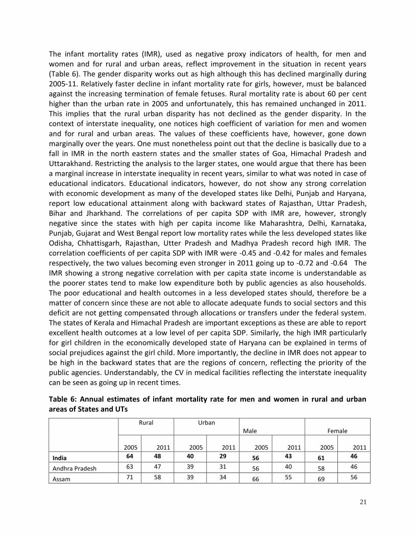
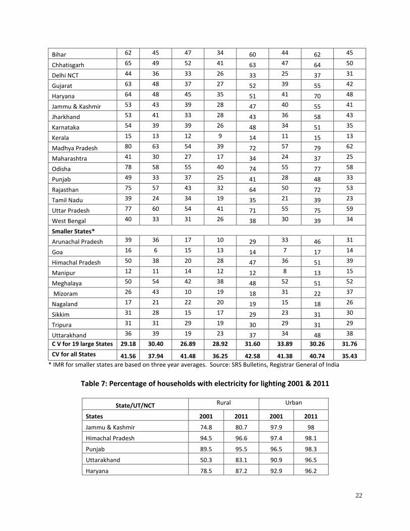
The infant mortality rates (IMR), used as negative proxy indicators of health, for men and women and for rural and urban areas, reflect improvement in the situation in recent years (Table 6). The gender disparity works out as high although this has declined marginally during 2005-11. Relatively faster decline in infant mortality rate for girls, however, must be balanced against the increasing termination of female fetuses. Rural mortality rate is about 60 per cent higher than the urban rate in 2005 and unfortunately, this has remained unchanged in 2011. This implies that the rural urban disparity has not declined as the gender disparity. In the context of interstate inequality, one notices high coefficient of variation for men and women and for rural and urban areas. The values of these coefficients have, however, gone down marginally over the years. One must nonetheless point out that the decline is basically due to a fall in IMR in the north eastern states and the smaller states of Goa, Himachal Pradesh and Uttarakhand. Restricting the analysis to the larger states, one would argue that there has been a marginal increase in interstate inequality in recent years, similar to what was noted in case of educational indicators. Educational indicators, however, do not show any strong correlation with economic development as many of the developed states like Delhi, Punjab and Haryana, report low educational attainment along with backward states of Rajasthan, Uttar Pradesh, Bihar and Jharkhand. The correlations of per capita SDP with IMR are, however, strongly negative since the states with high per capita income like Maharashtra, Delhi, Karnataka, Punjab, Gujarat and West Bengal report low mortality rates while the less developed states like Odisha, Chhattisgarh, Rajasthan, Utter Pradesh and Madhya Pradesh record high IMR. The correlation coefficients of per capita SDP with IMR were -0.45 and -0.42 for males and females respectively, the two values becoming even stronger in 2011 going up to -0.72 and -0.64 The IMR showing a strong negative correlation with per capita state income is understandable as the poorer states tend to make low expenditure both by public agencies as also households. The poor educational and health outcomes in a less developed states should, therefore be a matter of concern since these are not able to allocate adequate funds to social sectors and this deficit are not getting compensated through allocations or transfers under the federal system. The states of Kerala and Himachal Pradesh are important exceptions as these are able to report excellent health outcomes at a low level of per capita SDP. Similarly, the high IMR particularly for girl children in the economically developed state of Haryana can be explained in terms of social prejudices against the girl child. More importantly, the decline in IMR does not appear to be high in the backward states that are the regions of concern, reflecting the priority of the public agencies. Understandably, the CV in medical facilities reflecting the interstate inequality can be seen as going up in recent times.
Table 6: Annual estimates of infant mortality rate for men and women in rural and urban areas of States and UTs
Rural
Urban Male Female
2005 2011 2005 2011 2005 2011 2005 2011
India 64 48 40 29 56 43 61 46
Andhra Pradesh 63 47 39 31 56 40 58 46
Assam 71 58 39 34 66 55 69 56
22
Bihar 62 45 47 34 60 44 62 45
Chhatisgarh 65 49 52 41 63 47 64 50
Delhi NCT 44 36 33 26 33 25 37 31
Gujarat 63 48 37 27 52 39 55 42
Haryana 64 48 45 35 51 41 70 48
Jammu & Kashmir 53 43 39 28 47 40 55 41
Jharkhand 53 41 33 28 43 36 58 43
Karnataka 54 39 39 26 48 34 51 35
Kerala 15 13 12 9 14 11 15 13
Madhya Pradesh 80 63 54 39 72 57 79 62
Maharashtra 41 30 27 17 34 24 37 25
Odisha 78 58 55 40 74 55 77 58
Punjab 49 33 37 25 41 28 48 33
Rajasthan 75 57 43 32 64 50 72 53
Tamil Nadu 39 24 34 19 35 21 39 23
Uttar Pradesh 77 60 54 41 71 55 75 59
West Bengal 40 33 31 26 38 30 39 34
Smaller States*
Arunachal Pradesh 39 36 17 10 29 33 46 31
Goa 16 6 15 13 14 7 17 14
Himachal Pradesh 50 38 20 28 47 36 51 39
Manipur 12 11 14 12 12 8 13 15
Meghalaya 50 54 42 38 48 52 51 52
Mizoram 26 43 10 19 18 31 22 37
Nagaland 17 21 22 20 19 15 18 26
Sikkim 31 28 15 17 29 23 31 30
Tripura 31 31 29 19 30 29 31 29
Uttarakhand 36 39 19 23 37 34 48 38
C V for 19 large States 29.18 30.40 26.89 28.92 31.60 33.89 30.26 31.76
CV for all States 41.56 37.94 41.48 36.25 42.58 41.38 40.74 35.43
* IMR for smaller states are based on three year averages. Source: SRS Bulletins, Registrar General of India
Table 7: Percentage of households with electricity for lighting 2001 & 2011
State/UT/NCT Rural Urban
States 2001 2011 2001 2011
Jammu & Kashmir 74.8 80.7 97.9 98
Himachal Pradesh 94.5 96.6 97.4 98.1
Punjab 89.5 95.5 96.5 98.3
Uttarakhand 50.3 83.1 90.9 96.5
Haryana 78.5 87.2 92.9 96.2
23
Delhi NCT 85.5 97.8 93.4 99.1
Rajasthan 44 58.3 89.6 93.9
Uttar Pradesh 19.8 23.8 79.9 81.4
Bihar 5.1 10.4 59.3 66.7
Sikkim 75 90.2 97.1 98.7
Arunachal Pradesh 44.5 55.5 89.4 96.0
Nagaland 56.9 75.2 90.3 97.4
Manipur 52.5 61.2 82 82.4
Mizoram 44.1 68.8 94.4 98.1
Tripura 31.8 59.5 86.4 91.6
Meghalaya 30.3 51.6 88.1 94.9
Assam 16.5 28.4 74.3 84.1
West Bengal 20.3 40.3 79.6 85.1
Jharkhand 10 32.3 75.6 88
Odisha 19.4 35.6 74.1 83.1
Chhattisgarh 46.1 70 82.9 93.7
Madhya Pradesh 62.3 58.3 92.3 92.7
Gujarat 72.1 85 93.4 97.2
Maharashtra 65.2 73.8 94.3 96.2
Andhra Pradesh 59.7 89.7 90 97.3
Karnataka 72.2 86.7 90.5 96.4
Goa 92.4 95.6 94.7 97.7
Kerala 65.5 92.1 84.3 97.0
Tamil Nadu 71.2 90.8 88 96.1
Puducherry UT 81 95.8 91.4 98.5
All India 43.5 55.3 87.6 92.7
Coefficient of variation (%) 47.75 36.29 9.88 7.91
Table 8: Percentage of households having source of drinking water away from the premises 2001 & 2011
State/UT Rural Urban
2001 2011 2001 2011
Jammu & Kashmir 32 29.4 6.1 5.1
Himachal Pradesh 14.3 10.2 6.3 3.6
Punjab 4.2 5.7 1.5 1.6
Uttarakhand 20.5 20.1 5.2 3.5
Haryana 26.6 16.2 7.5 5.1
Delhi NCT 17.1 10.4 6.3 6.1
Rajasthan 28.6 31.9 8.2 7.7
24
Uttar Pradesh 11.3 14.1 5.4 5.2
Bihar 12.6 12.6 8.6 7
Sikkim 20.9 22.8 2.8 4.5
Arunachal Pradesh 19.8 26.4 11.4 7.3
Nagaland 33.5 31.4 21.1 20.7
Manipur 33.6 40.7 22.6 32.1
Mizoram 37.9 32.1 19.4 13.3
Tripura 31.4 39.6 9.9 13.7
Meghalaya 32.3 37.9 17.1 13.9
Assam 24.5 20.4 10.5 8.4
West Bengal 20.4 31.5 11.9 16.1
Jharkhand 26.7 36.4 16.7 17.8
Odisha 32.4 38.5 20.9 18.5
Chhattisgarh 22.3 30.3 13.7 12.9
Madhya Pradesh 27.3 36.1 15.3 14.5
Gujarat 20.8 18.5 6.5 4.8
Maharashtra 17.2 19.6 5.7 5.2
Andhra Pradesh 21.9 23.9 13.5 10.3
Karnataka 26.1 24.8 13.8 8.5
Goa 14.3 8.2 8 2.7
Kerala 13.5 10.8 7.4 5.2
Tamil Nadu 13.3 8.2 10.4 5.7
Puducherry UT 4.7 2.1 3.8 0.7
All India 19.5 22.1 9.4 8.1
Coefficient of variation (%) 39.52 49.34 54.11 72.89
CV ( Excluding Delhi & Goa) 39.29 46.31 54.03 71.18
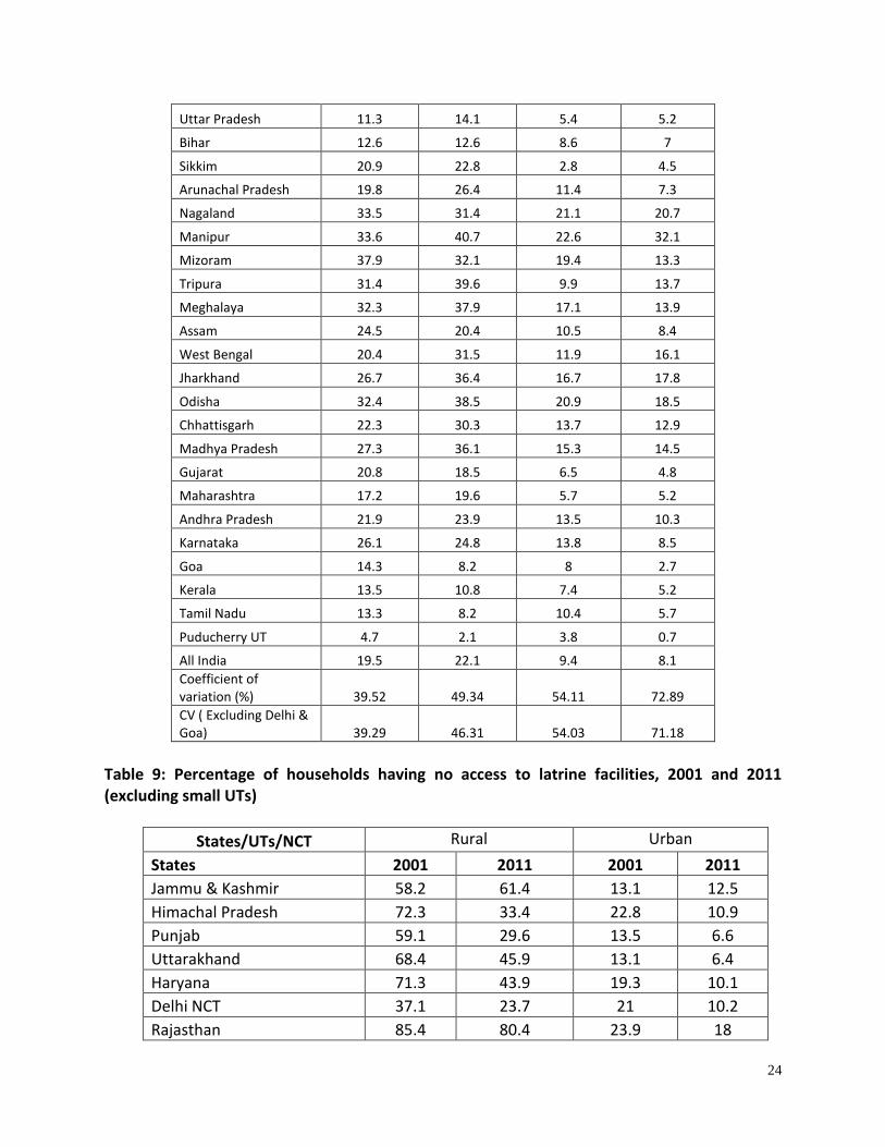
Table 9: Percentage of households having no access to latrine facilities, 2001 and 2011 (excluding small UTs)
States/UTs/NCT Rural Urban
States 2001 2011 2001 2011
Jammu & Kashmir 58.2 61.4 13.1 12.5
Himachal Pradesh 72.3 33.4 22.8 10.9
Punjab 59.1 29.6 13.5 6.6
Uttarakhand 68.4 45.9 13.1 6.4
Haryana 71.3 43.9 19.3 10.1
Delhi NCT 37.1 23.7 21 10.2
Rajasthan 85.4 80.4 23.9 18

25
Uttar Pradesh 80.8 78.2 20 16.9
Bihar 86.1 82.4 30.3 31
Sikkim 40.6 15.9 8.2 4.8
Arunachal Pradesh 52.7 47.3 13 10.5
Nagaland 35.4 30.8 5.9 5.4
Manipur 22.5 14 4.7 4.2
Mizoram 20.3 15.4 2 1.5
Tripura 22.1 18.5 3 2.1
Meghalaya 59.9 46.1 8.4 4.3
Assam 40.4 40.4 5.4 6.3
West Bengal 73.1 53.3 15.2 15
Jharkhand 93.4 92.4 33.3 32.8
Odisha 92.3 85.9 40.3 35.2
Chhattisgarh 94.8 85.5 47.4 39.8
Madhya Pradesh 91.1 86.9 32.3 25.8
Gujarat 78.3 67 19.5 12.3
Maharashtra 81.8 62 41.9 28.7
Andhra Pradesh 81.9 67.8 21.9 13.9
Karnataka 82.6 71.6 24.8 15.1
Goa 51.8 29.1 30.8 14.7
Kerala 18.7 6.8 8 2.6
Tamil Nadu 85.6 76.8 35.7 24.9
Puducherry UT 78.6 61 35 18
All India 78.1 69.3 26.3 18.6
C V (%) 38.01 50.02 61.54 72.27
CV ( Excluding Delhi & Goa) 37.51 48.25 64.22 73.86
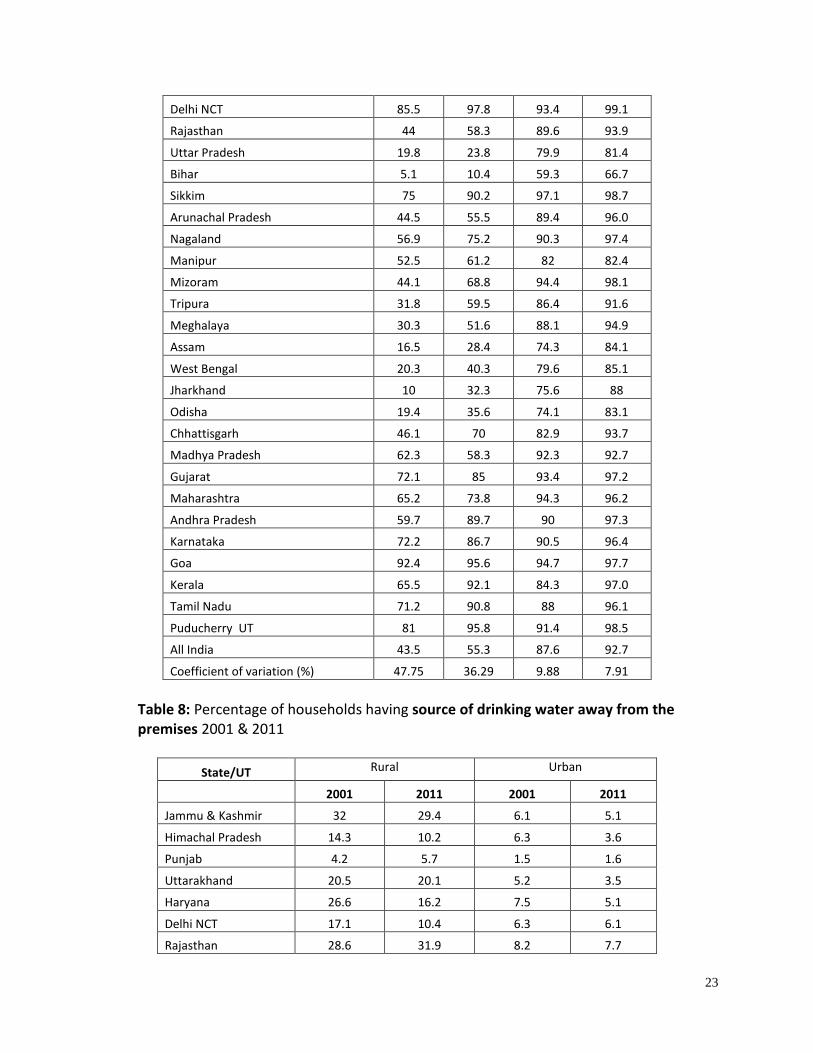
Access to Basic Amenities Sanitation and other civic amenities in a state would have a positive effect on health of the people, particularly the children. An attempt has therefore been made to determine to analyse the access of the households to latrine and drinking water facilities at the state level and across social groups. The percentage of households having electricity connection has gone up significantly both in rural and urban areas (Table 7). The increase is higher in the former which has reduced the rural urban inequality over the past decade. The inter-state inequality too has recorded a noticeable reduction, the decline in coefficient of variation being higher in rural than urban areas. This would be considered a positive step towards inclusive growth in the country. Unfortunately, the same cannot be said regarding water supply and sanitation facilities. The reduction in the

26
percentage of households not having safe drinking water facility (Table 8) and toilet (Table 9) within the premise is much less than that of households not having electricity. Furthermore, the interstate inequality has gone up significantly in case of both water as well as sanitation facilities. It is a matter of anxiety that the level of income of the states determine the access to toilet facilities and safe drinking water, the correlations being 0.72 and 0.43 respectively. This should be a matter of serious concern since not having access to these basic amenities in the economically backward states would have a direct bearing on the health status of the family members, particularly the infant mortality rates.
4. Inequalities and Inequality across Social, Religious and Gender Groups
Consumption Expenditure
The discussion on the growth scenario will be incomplete without considering the fact that the benefits do not accrue uniformly also across socio-religious categories. The historically underprivileged scheduled caste and scheduled tribe population are often noted as recording slower improvement over time in multiple economic and social dimensions. The sharpening of inequalities across the states, as discussed above, would also affect these socio-economic groups differently. Furthermore, the deprivation of Muslims and discrimination against them in labour market and certain social spheres is also a matter of serious policy concern. The Prime Minister’s High Level Committee (Sachar Committee 2006), probing into this aspect has shown that the gaps in economic wellbeing between Muslims and the average population are very high, more so in case of urban areas and women than for rural areas and men. Various programs of the government including that of the Reserve Bank of India under the Prime Minister’s 15-point programme have not made much impact on their conditions.
Given the differential access to labour and capital market of different castes and communities, an attempt is made here to analyse the trends and pattern per capita consumption expenditure - a summary measure of economic wellbeing - to assess the magnitude inter group inequality in the country. Muslims, Christians, Sikhs and Buddhists are India’s prominent minority communities, accounting for 140 million or about 18 per cent of the country’s billion-plus population. Muslims constitute about 75 per cent of this minority population. Following the classification system adopted by the Sachar Committee, Hindus have been placed in 3 categories – SCs, STs and Others for the analysis in this section. However, for comparability with other sections, figures for total SCs and STs have also been computed. Other religious groups (ORG) include all non Hindu religious groups except Muslims but include non-Hindu SC & ST population that are very small. The people in the first five categories thus add up to the total population with no overlap between any two categories.
27
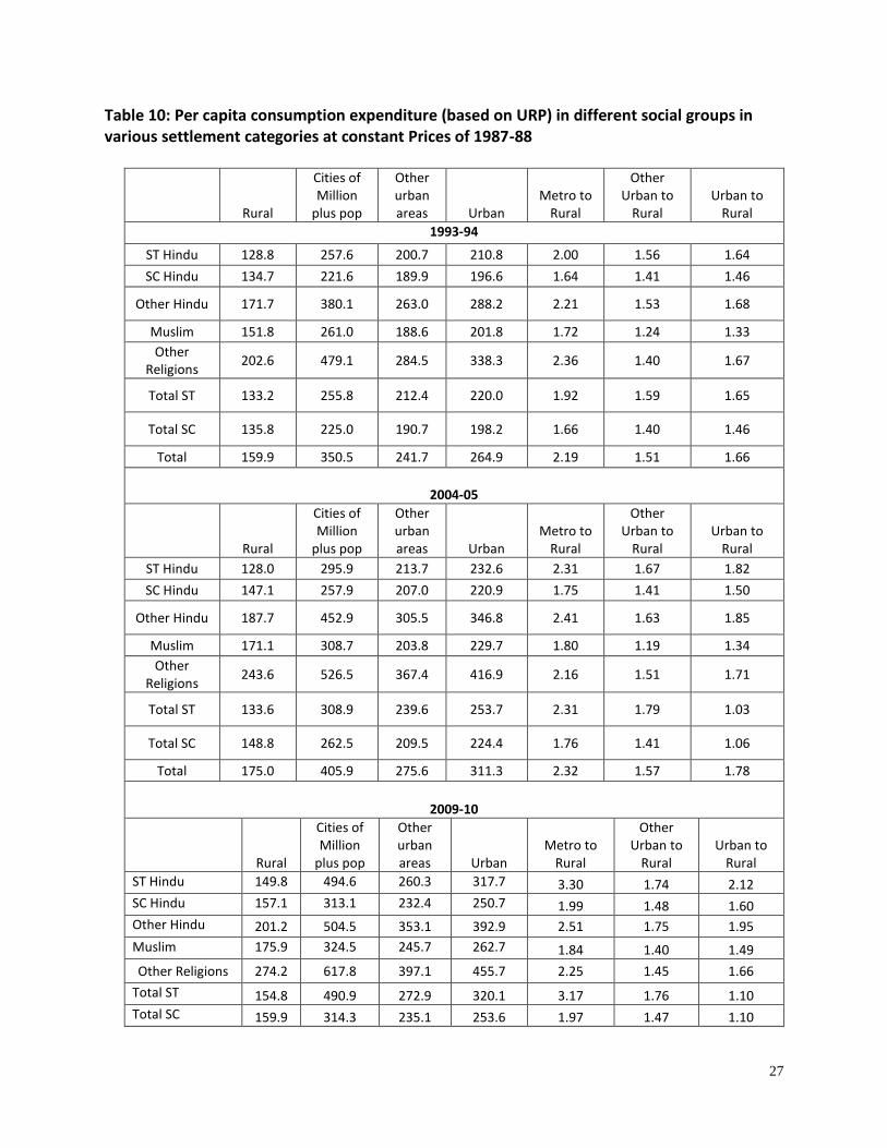
Table 10: Per capita consumption expenditure (based on URP) in different social groups in various settlement categories at constant Prices of 1987-88
Rural
Cities of Million
plus pop
Other urban areas Urban
Metro to Rural
Other Urban to
Rural Urban to
Rural
1993-94
ST Hindu 128.8 257.6 200.7 210.8 2.00 1.56 1.64
SC Hindu 134.7 221.6 189.9 196.6 1.64 1.41 1.46
Other Hindu 171.7 380.1 263.0 288.2 2.21 1.53 1.68
Muslim 151.8 261.0 188.6 201.8 1.72 1.24 1.33
Other Religions
202.6 479.1 284.5 338.3 2.36 1.40 1.67
Total ST 133.2 255.8 212.4 220.0 1.92 1.59 1.65
Total SC 135.8 225.0 190.7 198.2 1.66 1.40 1.46
Total 159.9 350.5 241.7 264.9 2.19 1.51 1.66
2004-05
Rural
Cities of Million
plus pop
Other urban areas Urban
Metro to Rural
Other Urban to
Rural Urban to
Rural
ST Hindu 128.0 295.9 213.7 232.6 2.31 1.67 1.82
SC Hindu 147.1 257.9 207.0 220.9 1.75 1.41 1.50
Other Hindu 187.7 452.9 305.5 346.8 2.41 1.63 1.85
Muslim 171.1 308.7 203.8 229.7 1.80 1.19 1.34
Other Religions
243.6 526.5 367.4 416.9 2.16 1.51 1.71
Total ST 133.6 308.9 239.6 253.7 2.31 1.79 1.03
Total SC 148.8 262.5 209.5 224.4 1.76 1.41 1.06
Total 175.0 405.9 275.6 311.3 2.32 1.57 1.78
2009-10
Rural
Cities of Million
plus pop
Other urban areas Urban
Metro to Rural
Other Urban to
Rural Urban to
Rural
ST Hindu 149.8 494.6 260.3 317.7 3.30 1.74 2.12
SC Hindu 157.1 313.1 232.4 250.7 1.99 1.48 1.60
Other Hindu 201.2 504.5 353.1 392.9 2.51 1.75 1.95
Muslim 175.9 324.5 245.7 262.7 1.84 1.40 1.49
Other Religions 274.2 617.8 397.1 455.7 2.25 1.45 1.66
Total ST 154.8 490.9 272.9 320.1 3.17 1.76 1.10
Total SC 159.9 314.3 235.1 253.6 1.97 1.47 1.10
28
Total 187.8 463.9 318.7 355.0 2.47 1.70 1.89
* derived from CPI for agricultural labourers with base 1986-87=100 # derived from CPI for urban non-manual employees with base 1984-85=100
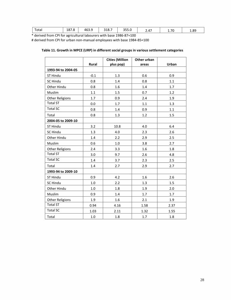
Table 11. Growth in MPCE (URP) in different social groups in various settlement categories
Rural Cities (Million
plus pop) Other urban
areas Urban
1993-94 to 2004-05
ST Hindu -0.1 1.3 0.6 0.9
SC Hindu 0.8 1.4 0.8 1.1
Other Hindu 0.8 1.6 1.4 1.7
Muslim 1.1 1.5 0.7 1.2
Other Religions 1.7 0.9 2.4 1.9
Total ST 0.0 1.7 1.1 1.3
Total SC 0.8 1.4 0.9 1.1
Total 0.8 1.3 1.2 1.5
2004-05 to 2009-10
ST Hindu 3.2 10.8 4.0 6.4
SC Hindu 1.3 4.0 2.3 2.6
Other Hindu 1.4 2.2 2.9 2.5
Muslim 0.6 1.0 3.8 2.7
Other Religions 2.4 3.3 1.6 1.8
Total ST 3.0 9.7 2.6 4.8
Total SC 1.4 3.7 2.3 2.5
Total 1.4 2.7 2.9 2.7
1993-94 to 2009-10
ST Hindu 0.9 4.2 1.6 2.6
SC Hindu 1.0 2.2 1.3 1.5
Other Hindu 1.0 1.8 1.9 2.0
Muslim 0.9 1.4 1.7 1.7
Other Religions 1.9 1.6 2.1 1.9
Total ST 0.94 4.16 1.58 2.37
Total SC 1.03 2.11 1.32 1.55
Total 1.0 1.8 1.7 1.8
29
0
200
400
600
800
1000
1200
1400
1600
ST Hindu SC Hindu OtherHindu
Muslim OtherReligions
All India
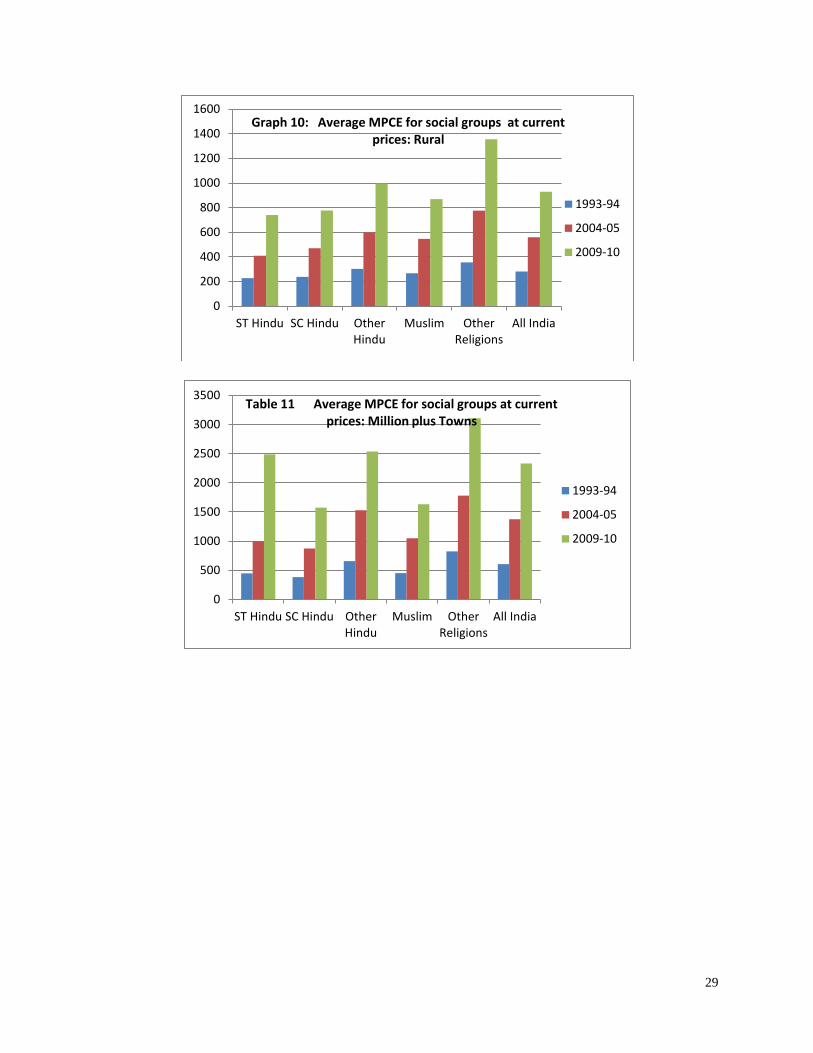
Graph 10: Average MPCE for social groups at current prices: Rural
1993-94
2004-05
2009-10
0
500
1000
1500
2000
2500
3000
3500
ST Hindu SC Hindu OtherHindu
Muslim OtherReligions
All India
Table 11 Average MPCE for social groups at current prices: Million plus Towns
1993-94
2004-05
2009-10

30
The percentage of Muslims to total population in urban areas is slightly higher than that in rural areas. This is due to historical factors, the seat of governance during the Mughal period being the large cities of today. The growth of population among Muslims (also Sikhs) is higher than the national growth rate in recent decades, particularly in rural areas, but that has to be understood and explained in terms of their socio-economic characteristics rather than religious identities. Further, there has been a decline in their growth rate during the nineties (the information for the decade 2001-11 are yet to be released), compared to the previous decade. Rural-Urban migration for both Muslims and Sikhs has declined as inferred from their declining share in urban population.
Economic wellbeing of population, in different social categories in rural areas, towns and metro (million plus population) cities, has been measured using the large sample data on consumption expenditure from NSS over the period from 1993-94 to 2009-10 at the constant prices of 1987-88. It is seen that the ST Hindus are at the bottom of the ladder in rural areas, followed by SC (Table 10 and Graph 10) at all the three time points. In urban areas, however, STs are better off than both SCs and Muslims (Table 10 and Graphs 11 and 12). This can be attributed to the fact that the STs do not move out of rural areas due to economic distress or seasonality, owing to their strong socio-cultural bonds and consequently their rate of out migration is low. They migrate out mostly induced by governmental schemes and programmes and therefore record the maximum relative gain through their movement. The ratio of urban to rural figure for the ST is similar to the average figure in 1993-94 and is the highest among all social groups in 2009-10. This can be attributed to their very high growth in consumption expenditure in urban areas, particularly in metro cities, during 1993-2009, partly due to the low figure in the base year. The growth in consumption in rural areas is about the same across communities except for the ORG which recorded a significantly higher growth rate than the others.
SC Hindus record marginally higher consumption expenditure than the STs in rural areas but in urban areas, it is the other way round. The annual compound growth in consumption for the SCs during 1993-2009 (1 per cent per annum) is marginally higher than that of STs but is at par
0
500
1000
1500
2000
2500
ST Hindu SC Hindu OtherHindu
Muslim OtherReligions
All India
Table 13 Average MPCE for social groups at current prices : Non Million plus cities and Towns
1993-94
2004-05
2009-10
31
with that of other Hindus or total population. Importantly, ST-SC gap in urban areas has gone up significantly particularly in metro cities, while the gap in rural areas has remained the same. SCs have done better than other Hindus and Muslims in metro cities but much worse than them in small urban areas.
Muslims are at a slightly higher level of consumption compared to SC population in rural areas as also in small and large urban centres, in both the years. In rural areas, their consumption expenditure is 95 per cent of the rural average figure in 1993-94 and remains stable over the years. Muslim-non Muslim gap in rural areas work out as low but go up in urban centres, particularly in metro cities. The low gap in rural areas could be attributed to their being outside agriculture - into small manufacturing and service activities - where earnings are higher. Unfortunately, Muslims seem to be benefiting the least by shifting to smaller or larger urban centres relative to the other communities (Table 10), as may be inferred from the low metro to rural and urban to rural ratios in Table 10. Importantly, the growth rates in consumption for Muslims are less than the average for other religious groups in all settlement types (Table 11). Furthermore, the divergence between the two is the highest in metro cities, wherein the Muslims saw the lowest growth in consumption during 1993-2009 in relative terms.
The non SC/ST Hindus are better off than all other groups except the other religious groups (ORG) that include Christians, Parsis, Buddhists etc., in all settlement categories at both the time points. The growth in consumption expenditure in case of the former, however, is significantly below that of the ORG in rural areas and small towns. In metro cities, however, the opposite is the case. On the whole, the upper caste Hindus and non Muslim minority groups have reported higher levels of consumption in the base year and have also improved their expenditure figures over the years much more than the other groups. It is only in metropolitan cities that the STs and SCs have been able to benefit relatively more than the general population. Furthermore, urbanisation improves economic wellbeing of all but the impact varies across social groups. The maximum benefit comes to STs and upper caste Hindus followed by ORG, as one would infer from the ratio of the urban to rural figures (Table 10). Muslims come at the bottom in the context of improvement through movement to urban areas.
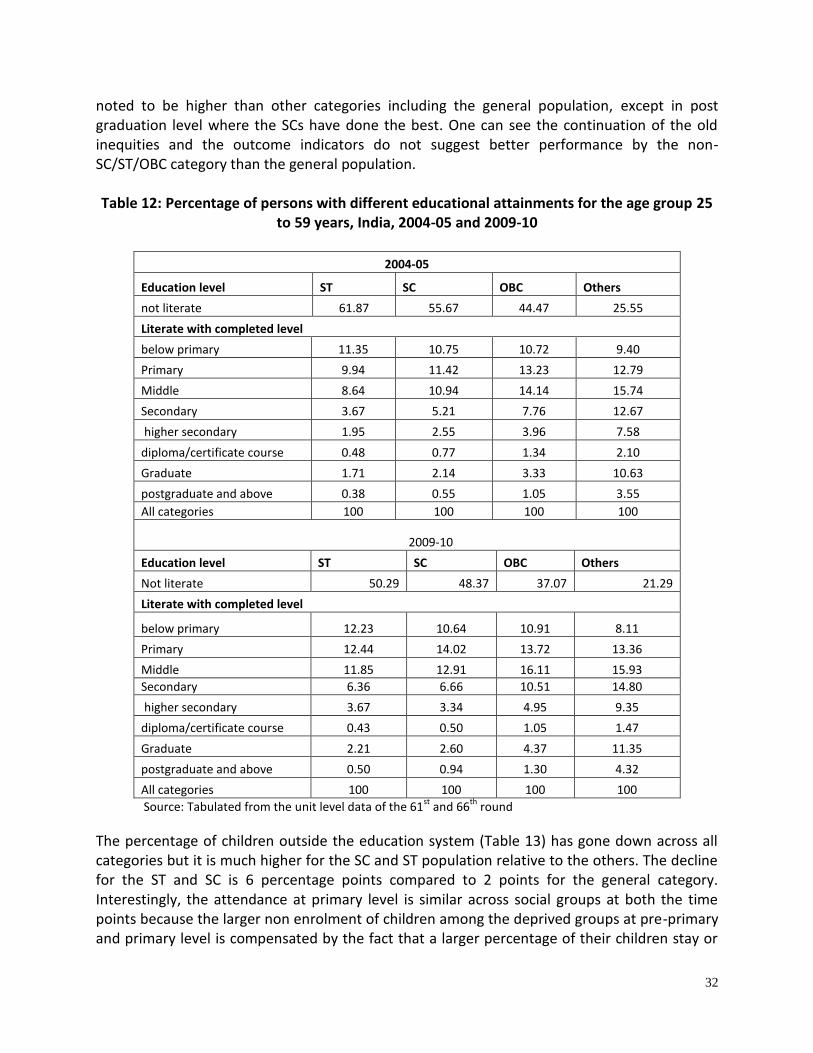
Education and Health In the context of educational attainment for persons in 25-59 age group, information from the two NSS rounds pertaining to 2004-05 and 2009-10 show (Table 12) that there is a high level of deprivation for the ST, SC and OBC population, in this order. This is inferred from the high level of illiteracy among them, two and a half times compared to the general category. Nevertheless, there have been progressive improvements over time in the education level for all social groups. Persons in the general category can still be noted as having significantly higher levels of attainment, compared to ST and SC population in 2009-10. Over 26 percent of the former have education level of higher secondary and above while this percentage figure is only 7 for ST and SC and 12 for the other backward castes. The improvement for the ST during 2004-09 can be
32
noted to be higher than other categories including the general population, except in post graduation level where the SCs have done the best. One can see the continuation of the old inequities and the outcome indicators do not suggest better performance by the non-SC/ST/OBC category than the general population. Table 12: Percentage of persons with different educational attainments for the age group 25
to 59 years, India, 2004-05 and 2009-10
2004-05
Education level ST SC OBC Others
not literate 61.87 55.67 44.47 25.55
Literate with completed level
below primary 11.35 10.75 10.72 9.40
Primary 9.94 11.42 13.23 12.79
Middle 8.64 10.94 14.14 15.74
Secondary 3.67 5.21 7.76 12.67
higher secondary 1.95 2.55 3.96 7.58
diploma/certificate course 0.48 0.77 1.34 2.10
Graduate 1.71 2.14 3.33 10.63
postgraduate and above 0.38 0.55 1.05 3.55
All categories 100 100 100 100
2009-10
Education level ST SC OBC Others
Not literate 50.29 48.37 37.07 21.29
Literate with completed level
below primary 12.23 10.64 10.91 8.11
Primary 12.44 14.02 13.72 13.36
Middle 11.85 12.91 16.11 15.93
Secondary 6.36 6.66 10.51 14.80
higher secondary 3.67 3.34 4.95 9.35
diploma/certificate course 0.43 0.50 1.05 1.47
Graduate 2.21 2.60 4.37 11.35
postgraduate and above 0.50 0.94 1.30 4.32
All categories 100 100 100 100
Source: Tabulated from the unit level data of the 61st
and 66th
round
The percentage of children outside the education system (Table 13) has gone down across all categories but it is much higher for the SC and ST population relative to the others. The decline for the ST and SC is 6 percentage points compared to 2 points for the general category. Interestingly, the attendance at primary level is similar across social groups at both the time points because the larger non enrolment of children among the deprived groups at pre-primary and primary level is compensated by the fact that a larger percentage of their children stay or

33
enroll at that level, instead of going to higher levels. The percentage of children in the middle and secondary school, however, are much lower for the SC, ST population than the other groups. The disparity however has gone down over the years. There has been an increase in school attendance at higher levels due to a decline in the percentage of children dropping out of the school at the age of 9 or 10 years. This increase has been higher for the socially deprived groups compared to the others, confirming the proposition of increase in equity within the formal education system. Table 13 Percentage of children in Current attendance (for age group 5 to 14), NSS 61st round, 2004-05 and 2009-10
2004-05
ST SC OBC Others
Currently attending in: Pre-primary and Primary
53.43 54.61 55.14 54.52
Currently attending in: Middle 16.57 19.06 20.63 24.72
Currently attending in: Secondary 3.43 4.81 6.49 8.64
Not in the education system 26.57 21.52 17.74 12.12
2009-10
ST SC OBC Others
Currently attending in: Pre-primary 52.36 53.66 54.05 53.13
Currently attending in: Middle 21.22 23.53 23.31 26.19
Currently attending in: Secondary 7.20 7.56 9.23 10.13
Not in the education system 19.22 15.25 13.41 10.55
Source: NSS 61st
and 66th
round survey data. As an outcome indicator of health system, infant mortality rate is often considered as the most appropriate for India, although it reflects the combined impact of factors like access to health care facilities, educational level and economic well being of the people in a region. In the Table below, the IMR for different religious groups (Table 14) show that it is low for Sikh, Buddhists and Christians in rural areas compared to Hindus and Muslims. Among the social groups, the IMR is the highest for SC, followed by the ST. However the IMR for all categories are still way above that observed in developed countries. Table 14: Infant mortality rates for socio-religious groups for 1998-99 and 2005-06
Infant mortality rates for socio-religious groups: All India, 1998-99
Rural Urban Total
Hindu 82.8 53.3 77.1
Muslim 67.5 39.9 58.8
Christian 53.9 37.5 49.2
Sikh 56.8 40.6 53.3
Buddhist/Neo 76.9 26.7 53.6

34
Buddhist
Others 91.0 26.7 80.3
ST 86.9 57.6 84.2
SC 88.1 60.4 83.0
OBC 82.2 51.2 76.0
Others 69.3 43.5 61.8
Infant mortality rates for socio-religious groups: All India, 2005-06
Rural Urban Total
Hindu 63.0 44.3 58.5
Muslim 60.4 35.5 52.4
Christian 54.8 16.3 41.7
Sikh 46.0 Not Reported 45.6
Buddhist 46.6 Not Reported 52.8
Others 86.7 Not Reported 84.6
ST 63.9 43.8 62.1
SC 71.0 50.7 66.4
OBC 61.1 42.2 56.6
Others 55.7 36.1 48.9 Source: Table 6.4, NFHS-2 and Table 7.2, NFHS-3, All India reports
Sanitation and Water Supply
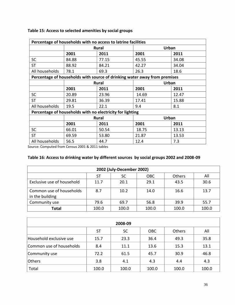
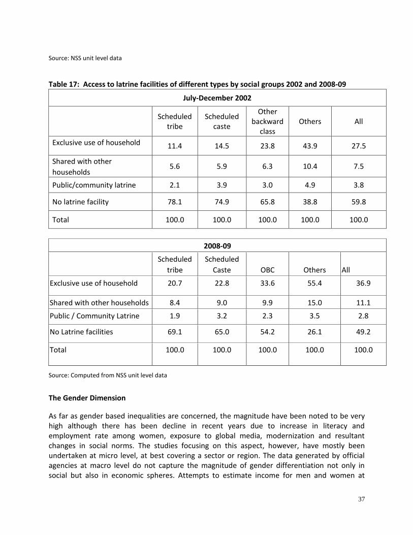
The percentage of households having no toilet facility is extremely high in rural areas, as revealed from the Population Census (Table 15). However, against the 70 per cent for rural India, the figures are as high as 77 per cent for SC and 84 per cent for ST in 2011. In urban India, the deficits are lower and there is no difference between the figures for SC and ST population. In case of households having drinking water sources outside the premise, the figures are less but the SC and ST figures are much larger compared to the national average. Similar is the pattern across social groups in case of the percentage of households not having electricity for lighting, but here there is no difference between ST SC population in urban areas, as noted in case of toilet facilities. An identical pattern emerges from the NSS data for the years 2002 and 2008-09 (Table 16 & 17)). The percentage of households having drinking water facility for exclusive use is very low in case of the ST and SC population, compared to “others” category. The ST-SC gap is very high in case of drinking water but low for toilet facility. The access to both is better for the OBC and for the general category, the figures are even higher. The outcome indicators seem to suggest some progressivity in the provision of drinking water as the deprived social groups like ST and OBC report higher improvement in accessing drinking water for exclusive use. However, the improvements, not much in favour of SC population as their dependence on community facility
35
remains very high in 2008-09. A similar picture emerges from for the access to toilet facilities from the NSS data, the SC, ST and OBC reporting much lower figures for households having toilets for exclusive use that the others category. The improvements over the recent years, however, have been much more in favour of the deprived social groups than in case of drinking water facilities.
36
Table 15: Access to selected amenities by social groups
Percentage of households with no access to latrine facilities
Rural Urban
2001 2011 2001 2011
SC 84.88 77.15 45.55 34.08
ST 88.92 84.21 42.27 34.04
All households 78.1 69.3 26.3 18.6
Percentage of households with source of drinking water away from premises
Rural Urban
2001 2011 2001 2011
SC 20.89 23.96 14.69 12.47
ST 29.81 36.39 17.41 15.88
All households 19.5 22.1 9.4 8.1
Percentage of households with no electricity for lighting
Rural Urban
2001 2011 2001 2011
SC 66.01 50.54 18.75 13.13
ST 69.59 53.80 21.87 13.53
All households 56.5 44.7 12.4 7.3 Source: Computed from Census 2001 & 2011 tables
Table 16: Access to drinking water by different sources by social groups 2002 and 2008-09
2002 (July-December 2002)
ST SC OBC Others All
Exclusive use of household 11.7 20.1 29.1 43.5 30.6
Common use of households in the building
8.7 10.2 14.0 16.6 13.7
Community use 79.6 69.7 56.8 39.9 55.7
Total 100.0 100.0 100.0 100.0 100.0
2008-09
ST SC OBC Others All
Household exclusive use 15.7 23.3 36.4 49.3 35.8
Common use of households 8.4 11.1 13.6 15.3 13.1
Community use 72.2 61.5 45.7 30.9 46.8
Others 3.8 4.1 4.3 4.4 4.3
Total 100.0 100.0 100.0 100.0 100.0
37
Source: NSS unit level data
Table 17: Access to latrine facilities of different types by social groups 2002 and 2008-09
July-December 2002
Scheduled
tribe Scheduled
caste
Other backward
class Others All
Exclusive use of household 11.4 14.5 23.8 43.9 27.5
Shared with other
households 5.6 5.9 6.3 10.4 7.5
Public/community latrine 2.1 3.9 3.0 4.9 3.8
No latrine facility 78.1 74.9 65.8 38.8 59.8
Total 100.0 100.0 100.0 100.0 100.0
2008-09
Scheduled
tribe
Scheduled
Caste OBC Others All
Exclusive use of household 20.7 22.8 33.6 55.4 36.9
Shared with other households 8.4 9.0 9.9 15.0 11.1
Public / Community Latrine 1.9 3.2 2.3 3.5 2.8
No Latrine facilities 69.1 65.0 54.2 26.1 49.2
Total 100.0 100.0 100.0 100.0 100.0
Source: Computed from NSS unit level data
The Gender Dimension
As far as gender based inequalities are concerned, the magnitude have been noted to be very high although there has been decline in recent years due to increase in literacy and employment rate among women, exposure to global media, modernization and resultant changes in social norms. The studies focusing on this aspect, however, have mostly been undertaken at micro level, at best covering a sector or region. The data generated by official agencies at macro level do not capture the magnitude of gender differentiation not only in social but also in economic spheres. Attempts to estimate income for men and women at

38
national and state levels, for example, are fraught with serious methodological and data related problems, making the results extremely tentative. The NSS provides data on consumption expenditure only at household level and there is no way by which one can disaggregate that by gender.
One can, nonetheless, focus on the gender dimension by bringing out differences in poverty levels between men and women headed households. The incidence of poverty is indeed much higher among the latter than the former. The Graphs 13 and 14 show how the number of women per 1000 men in different expenditure classes. One notes that the number goes down with increase in the level of consumption expenditure, both rural and urban areas. The highest sex ratio is recorded in the first quintile. At higher expenditure classes, the sex ratio tapers off
840
860
880
900
920
940
960
980
1000
0 500 1000 1500 2000 2500 3000
s
e
x
r
a
t
i
o
Monthly per capita expenditure
Graph 13: Average monthly percapita expenditure and sex ration for different deccile
classes ( NSS 66th round- RURAL)
840
860
880
900
920
940
960
980
1000
0 1000 2000 3000 4000 5000 6000
s
e
x
r
a
t
i
o
Monthly per capita expenditure
Graph 14: Average monthly perr capita expenditure and sex ratio for different decile classes (NSS 66th round _ URBAN)
39
and goes well below the average figure for the country. It is well-known that households tend to be headed by women often due to the exigency of the male earning member being dead or deserting the family. The probability of women headed households having a single earner and her getting lower earnings than a male in a similar job is high. The households below poverty line have higher female male ratio compared to the average households, both in urban and rural areas. Understandably, poverty among women would work out to be much higher than among men, even if one chooses to ignore the gender differences in consumption within the household.
5. Conclusions and a Perspective for Intervention An overview of the human development scenario at global level suggests that the serious deficits in the three dimensions, income, health and education, as identified by UNDP, can be attributed largely to the inequality existing within the countries. The loss in income index, reflecting intra country inequality, for the countries having high or very high level of human development, is high whereas that in education and health index are relatively low. For the countries in the middle category, the intra country inequality is higher but the increases in case of health and education are much higher than that in income inequality. In case of the less developed countries, the income inequality is less than that in the medium category but that in health and educational indices are extremely high. This implies that the less developed countries, besides reporting fairly high income inequality are also failing in ensuring good health conditions and access to education for all sections of their population. The pattern, emerging from the computation of the inequality adjusted indices for the three human development dimensions in India at the state level for the recent years confirms this pattern. The interstate inequality is very high for educational and health indices - more than twice that of the income index. The overview of the trend and pattern of economic growth across the states over the past two and a half decades reveals that the high growth in income and consumption expenditure have been associated with increase in regional inequalities. Despite systematic reduction in poverty both in rural and urban areas over the past three and a half decades, inequality has gone up - in rural areas, but more significantly in urban areas. Poverty has got concentrated in a few regions and social groups where poverty alleviation is likely to be more difficult in future years. The percentage of children outside the formal education system, despite a decline in recent years, works out as very high in 2009-10 both in rural and urban areas. Importantly, the R-U disparity in this indicator is not very high compared to that in the percentage of persons with secondary and higher education. By both the indicators, the situation has improved during 2005-10. What, however, is disturbing that the inequality in both the indicators across the states has gone up in both urban and rural areas. In case of the two indicators for males and females, one would argue that the situation has improved for both and that the gender disparity has gone down over the decade. In case for interstate inequality, however, the trend is the opposite. For men the inequality has gone up distinctly in both the indicators while for
40
women, it has gone up in case of children outside education system. For educational attainment for women, the inequality seems to have remained stable during 2001-11. The IMR shows a significant variation across the states, strongly correlated with their level of backwardness. Unfortunately, the decline in IMR is not high in the backward states, reflecting that the thrust of intervention has not been in the high priority regions. The interstate inequality in the health indicator can be seen as going up in recent times. Sanitation and drinking water facility in a state would have a positive effect on health of the people, particularly the children. The strong negative relationship of IMR and deficiencies in provision of the amenities with per capita SDP suggest that the less developed states have not been able to make adequate provision for the social sectors. Unfortunately, the deficiencies have not been made up through increased allocations from the federal funds. There exists significant disparity between ST, SC and general population on the one hand and Muslims compared with other religious groups. The level of consumption expenditure and growth therein during 1993-2009 has been very high in million plus cities, compared to small towns or rural areas for all socio-religious groups. STs, although are at a low level in villages, towns and metro cities, record the highest growth in expenditure in metro cities during the period under study. Rural urban migration for employment emerges as a tool of poverty alleviation. This, however, is noted to make a differential impact on a person or a household, depending on whether the movement is to a metro city or other urban centre and also on his/her socio-religious identity. Importantly, STs benefit much more than the other groups by shifting from rural to urban areas. The growth in consumption for the SCs has been similar to that of average in rural areas. This however is much less than the average in non metro cities while in metro cities, it is the other way round. Muslims, however, have benefitted less than the average in all settlement categories. There exists significant disparity between scheduled tribes and scheduled castes population in terms of educational attainment, STs being the most deprived category. There has, however, been a progressive improvement for all social groups, this in case of the STs is higher than the other groups. There is continuation of old inequities and there is no evidence of better performance by the non-SC/ST/OBC category than the general population. The access to drinking water and toilet facilities for exclusive use is low in case of the ST and SC population, the figure is higher for the OBC and still higher for the general category. There is no conscious policy in favour of the deprived social groups, smoothening out the inequalities, as the gains are similar across the social groups. As far as gender based inequalities are concerned, the magnitude have been noted to be very high although there has been decline in recent years due to increase in literacy and employment rate among women, exposure to global media, modernization and resultant changes in social norms. The number of women per 1000 men in different expenditure classes goes down with increase in the level of consumption expenditure, both rural and urban areas. The probability of women headed households having a single earner and her getting lower
41
earnings than a male in a similar job is high. The households below poverty line have higher female male ratio compared to the average households, both in urban and rural areas. Understandably, poverty among women is much higher than among men, even if one chooses to ignore the gender differences in consumption within the household. The high inequality in IMR across the states and its increasing trend over time should be a matter of serious policy concern. The inequalities in the provision of water and toilets across the states too have gone up in recent years. While the absence of basic amenities, particularly toilets, have a strong association with health facilities and both are negatively related to per capita income, one would argue that growth process will not address the problems of human development in less developed states that are not growing rapidly. Unless there are specific policies and interventions to address the issue of delivery of basic amenities and tacking the problem of health in backward regions and for the poor and vulnerable social groups, it would be impossible to achieve the concerned MDG targets even at the national levels.
42
References Ahluwalia, M. S. (2000): “Economic Performance of States in Post Reform Era”, Economic and Political Weekly, May. Ahmad, Ahsan and Narain Ashish (2008): “Towards Understanding Development in Lagging Regions of India” Paper Presented at the Conference on Growth and Development in the Lagging Regions of India, Administrative Staff College of India, Hyderabad. Cheng, J. J, Schuster-Wallace, C. J., Watt, S., Newbold, B. K. and Mente, A. (2012) : “An ecological quantification of the relationships between water, sanitation and infant, child, and maternal mortality” Environmental Health, 11:4 Suryanarayana, M. H., Agarwal, A. and Seeta Prabhu, K. (2011): Inequality- Adjusted Human Development Index for India’s States, United Nations Development Program, New Delhi Kundu, A. (2006): “Globalization and the Emerging Urban Structure: Regional Inequality and Population Mobility”, India: Social Development Report, Oxford, New Delhi. Kundu, A. and Mohanan, P. C. (2009): “Employment and Inequality Outcome in India” OECD Conference Paris, OECD Paris Kundu, A and N Sarangi (2006): “Urbanization and Growth Dynamics in India: An Analysis with Special Reference to Western and Central Regions” in R. Parthasarathy and S. Iyengar (eds.), Paradigm and Challenges for Western and Central India, New Delhi: Concept Publishing Company. ------------ (2007): “Migration, Employment Status and Poverty: An Analysis Across Urban Centres in India”, Economic and Political Weekly, Jan 27. Planning Commission (2009): Report of the Expert Committee to Reviw the Methodology for Estimation of Poverty, Government of India, New Delhi. Planning Commission (2005): Report of the Inter Ministry Task Group on Redressing Growing Regional Imbalances, Government of India, New Delhi. Planning Commission (2008a): Eleventh Five Year Plan 2007-2012, vol. I, Government of India, New Delhi Planning Commission (2008c): Working Group on Social Security set up for the Eleventh Five Year Plan, Government of India, Planning Commission, New Delhi. Prime Minister’s High Level Committee (2006): Social, Economic and Educational Status of the Muslim Community of India, Cabinet Secretariat Government of India, New Delhi
43
Registrar General (2008): SRS Bulletin, Sample Registration System, Vol. 43, no 1, Registrar General, Government of India. K. C. Sivaramakrishna, Kundu, A. and Singh, B. N. (2005): Handbook of Urbanisation, Oxford University Press, New Delhi United Nations Development Programme (2010): Human Development Report, The Real Wealth of Nations: Pathways to Human Development, United Nations Development Programme, New York. United Nations Development Programme (2013): Human Development Report, The Rise of the South: Human Progress in a Diverse World, United Nations Development Programme, New York.
44
United Nations Development Programme 55 Lodhi Estate, Post Box No. 3059 New Delhi 110003, India Tel: +91 11 46532333 Fax: +91 11 24627612 Email: [email protected] For more information: www.in.undp.org