Space Weather Services - Radio and Space Services

©Copyright Australian Government 2016 1

Space Weather Services

Introduction to HF radio propagation

1. The ionosphere

1.1 The regions of the ionosphere

In a region extending from a height of about 50 km to over 500 km, some of the atoms and

molecules are electrically charged (ionised) by radiation from the Sun. This region is called the

ionosphere (Figure 1.1).

Ionisation is the process in which electrically charged and neutral atoms and molecules gain or

lose electrons. Of specific interest to High Frequency (HF: 3 to 30 MHz) radio communications via

the ionosphere (sky wave) is the process where negatively charged electrons are stripped from

atoms and molecules to produce free electrons. While the ionosphere is named after the ions, it is

the free electrons which are essential for HF sky wave communications. The variations in density

of free electrons in the ionosphere cause HF radio waves to refract (bend), allowing the upper

atmosphere to be used as a reflector for communications between distant locations on the

ground.

The density of free electrons in the ionosphere is not uniform, regions of higher electron density

form at different altitudes. The height at which a particular frequency is refracted depends on the

electron density profile, with higher frequencies being refracted from the regions of higher

electron density. The region of highest electron density determines the highest frequency capable

of being refracted by the ionosphere.

In the day ionosphere there may be four regions present, the D, E, F1 and F2 regions. Their

approximate height ranges are:

D region 50 to 90 km

E region 90 to 140 km

F1 region 140 to 210 km

F2 region over 210 km

At night the D, E and F1 regions become depleted of free electrons so as to be insignificant to HF

sky wave. The F2 electron density also decreases during the course of the night so that lower

frequencies are required for use then; higher frequencies may actually penetrate the ionosphere.

At certain times during the solar cycle (mostly during winter at solar maximum) the daytime F1

and F2 regions merge. During these times and at night the F2 region is called the F region.

Only the E, F1 and F2 regions refract HF waves. The D region, through which an HF sky wave must

pass to reach the refracting region, absorbs the energy of the wave and reduces signal strength

(Section 1.5).

A thin, dense layer of electrons called sporadic E (Section 1.6) sometimes forms in the E region.

Sporadic E can occur day or night and is capable of refracting HF sky waves.


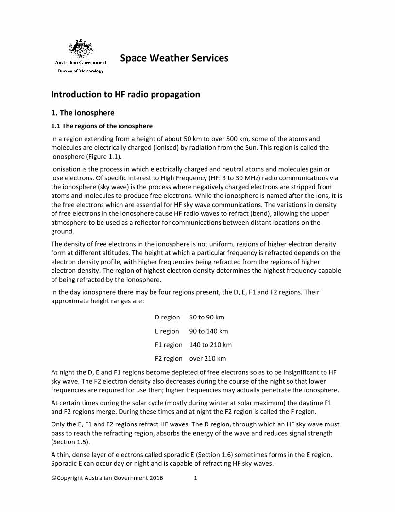
The F2 region is the most important region for HF sky wave propagation because:

• it is present 24 hours of the day;

• for long communication paths, its high altitude reduces the required number of hops;

• it usually refracts the highest frequencies in the HF range.

Figure 1.1 Day and night structure of the ionosphere. The black lines indicate electron density in

the day and night hemispheres. Electrons accumulate in layers within the regions. The highest

electron density normally occurs in the F region.

1.2 Production and loss of electrons in the ionosphere

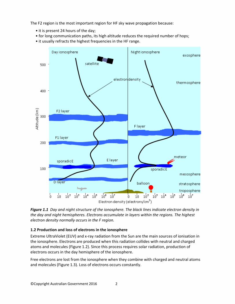
Extreme UltraViolet (EUV) and x-ray radiation from the Sun are the main sources of ionisation in

the ionosphere. Electrons are produced when this radiation collides with neutral and charged

atoms and molecules (Figure 1.2). Since this process requires solar radiation, production of

electrons occurs in the day hemisphere of the ionosphere.

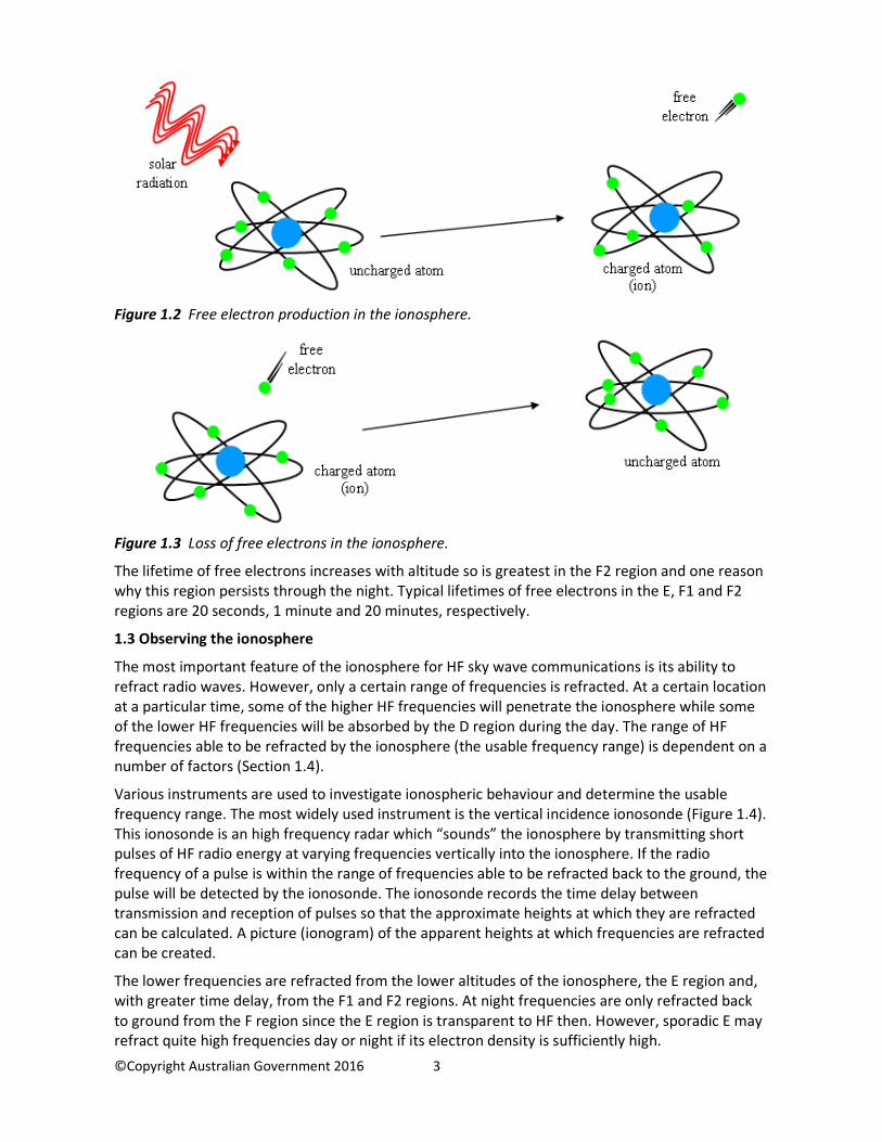
Free electrons are lost from the ionosphere when they combine with charged and neutral atoms

and molecules (Figure 1.3). Loss of electrons occurs constantly.


Figure 1.2 Free electron production in the ionosphere.

Figure 1.3 Loss of free electrons in the ionosphere.

The lifetime of free electrons increases with altitude so is greatest in the F2 region and one reason

why this region persists through the night. Typical lifetimes of free electrons in the E, F1 and F2

regions are 20 seconds, 1 minute and 20 minutes, respectively.

1.3 Observing the ionosphere

The most important feature of the ionosphere for HF sky wave communications is its ability to

refract radio waves. However, only a certain range of frequencies is refracted. At a certain location

at a particular time, some of the higher HF frequencies will penetrate the ionosphere while some

of the lower HF frequencies will be absorbed by the D region during the day. The range of HF

frequencies able to be refracted by the ionosphere (the usable frequency range) is dependent on a

number of factors (Section 1.4).

Various instruments are used to investigate ionospheric behaviour and determine the usable

frequency range. The most widely used instrument is the vertical incidence ionosonde (Figure 1.4).

This ionosonde is an high frequency radar which “sounds” the ionosphere by transmitting short

pulses of HF radio energy at varying frequencies vertically into the ionosphere. If the radio

frequency of a pulse is within the range of frequencies able to be refracted back to the ground, the

pulse will be detected by the ionosonde. The ionosonde records the time delay between

transmission and reception of pulses so that the approximate heights at which they are refracted

can be calculated. A picture (ionogram) of the apparent heights at which frequencies are refracted

can be created.

The lower frequencies are refracted from the lower altitudes of the ionosphere, the E region and,

with greater time delay, from the F1 and F2 regions. At night frequencies are only refracted back

to ground from the F region since the E region is transparent to HF then. However, sporadic E may

refract quite high frequencies day or night if its electron density is sufficiently high.


The ionosphere can also be sounded by oblique ionosondes which send pulses of radio energy

obliquely (at elevation angles off vertical) into the ionosphere and which are received at some

distant location. This type of sounder can monitor propagation on a particular sky wave path and

observe the various propagation modes supported (Section 2.4). Backscatter ionosondes also

transmit energy obliquely, which is refracted from the ionosphere and reflected off the ground

before returning via the ionosphere to the receiving antenna, which need not be co-located with

the transmitting antenna. This type of sounder is used for over-the-horizon radar.

Figure 1.4 Vertical incidence ionosonde operation. A picture of the ionosphere is produced by

measuring the travel time for each pulse of HF radio energy.

1.4 Ionospheric variations

The ionosphere is not a stable medium where a single frequency can be used throughout the year,

or even over 24 hours. The ionosphere varies with the solar cycle, the seasons, the sky wave path

used, and diurnally (through the day).

1.4.1 Variations due to the solar cycle

The Sun’s activity and radiation output slowly change over a period of about 9 to 14 years (the

“solar cycle”). The slow change in radiation output in turn affects the electron density profile of

the ionosphere and the range of HF frequencies usable on a sky wave path. At the commencement

of a solar cycle (solar minimum) radiation output is low, producing less ionisation and fewer

electrons in the ionosphere. Only the lower frequencies of the HF band are supported (refracted).

Radiation output at solar maximum is much greater leading to higher concentrations of electrons

in the ionosphere, and therefore, higher frequencies being supported. In fact, at very high solar

activity, frequencies in the VHF band which would normally penetrate the ionosphere may be


refracted and propagate as sky waves during the day on long paths. At solar maximum, the usable

HF frequency range expands usually offering a greater choice of frequencies from the available

frequency set. The solar cycle ends at the next solar minimum.

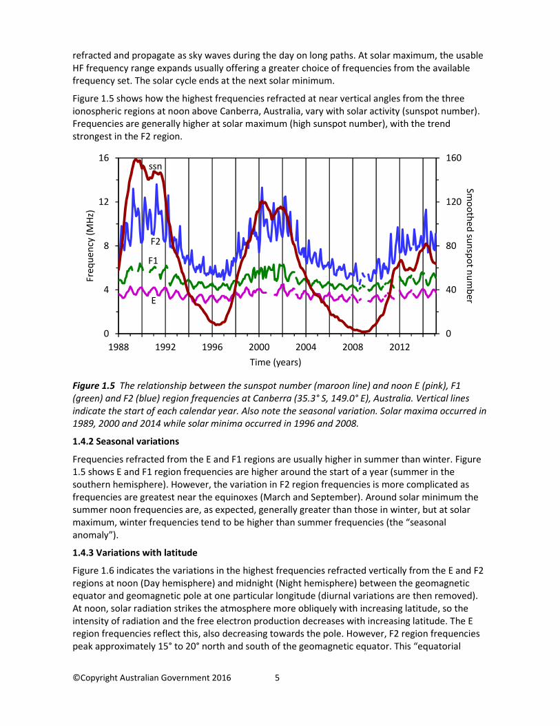
Figure 1.5 shows how the highest frequencies refracted at near vertical angles from the three

ionospheric regions at noon above Canberra, Australia, vary with solar activity (sunspot number).

Frequencies are generally higher at solar maximum (high sunspot number), with the trend

strongest in the F2 region.

Figure 1.5 The relationship between the sunspot number (maroon line) and noon E (pink), F1

(green) and F2 (blue) region frequencies at Canberra (35.3° S, 149.0° E), Australia. Vertical lines

indicate the start of each calendar year. Also note the seasonal variation. Solar maxima occurred in

1989, 2000 and 2014 while solar minima occurred in 1996 and 2008.

1.4.2 Seasonal variations

Frequencies refracted from the E and F1 regions are usually higher in summer than winter. Figure

1.5 shows E and F1 region frequencies are higher around the start of a year (summer in the

southern hemisphere). However, the variation in F2 region frequencies is more complicated as

frequencies are greatest near the equinoxes (March and September). Around solar minimum the

summer noon frequencies are, as expected, generally greater than those in winter, but at solar

maximum, winter frequencies tend to be higher than summer frequencies (the “seasonal

anomaly”).

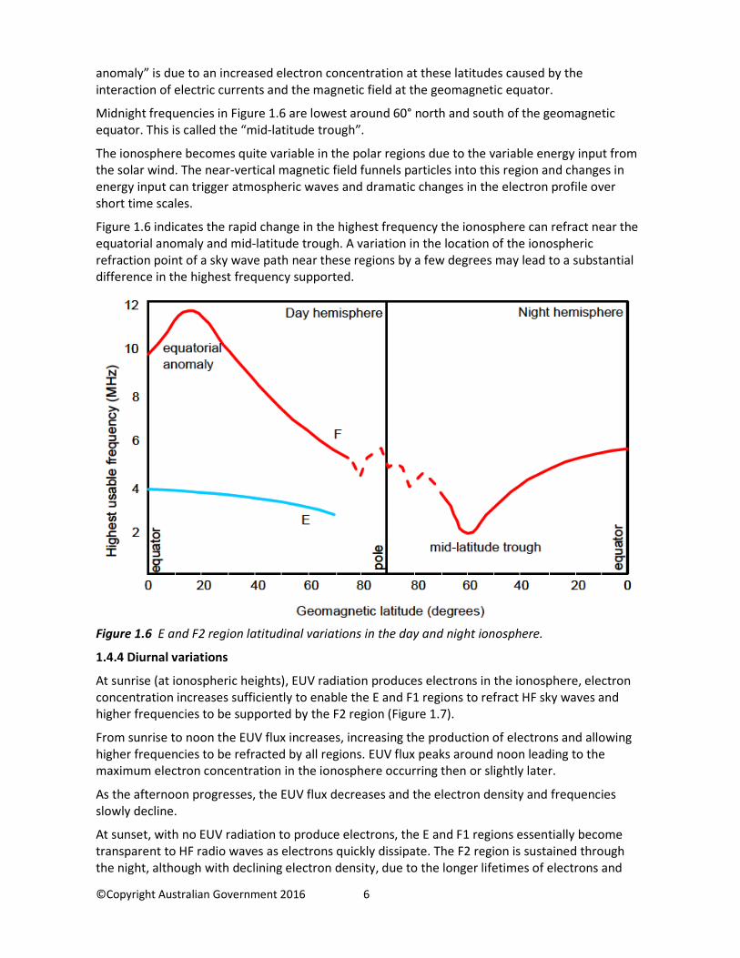
1.4.3 Variations with latitude

Figure 1.6 indicates the variations in the highest frequencies refracted vertically from the E and F2

regions at noon (Day hemisphere) and midnight (Night hemisphere) between the geomagnetic

equator and geomagnetic pole at one particular longitude (diurnal variations are then removed).

At noon, solar radiation strikes the atmosphere more obliquely with increasing latitude, so the

intensity of radiation and the free electron production decreases with increasing latitude. The E

region frequencies reflect this, also decreasing towards the pole. However, F2 region frequencies

peak approximately 15° to 20° north and south of the geomagnetic equator. This “equatorial

0

40

80

120

160

0

4

8

12

16

1988 1992 1996 2000 2004 2008 2012

Sm

oo

the

d su

nsp

ot n

um

be

rF

req

ue

ncy

(M

Hz)

Time (years)

ssn

F2

F1

E


anomaly” is due to an increased electron concentration at these latitudes caused by the

interaction of electric currents and the magnetic field at the geomagnetic equator.

Midnight frequencies in Figure 1.6 are lowest around 60° north and south of the geomagnetic

equator. This is called the “mid-latitude trough”.

The ionosphere becomes quite variable in the polar regions due to the variable energy input from

the solar wind. The near-vertical magnetic field funnels particles into this region and changes in

energy input can trigger atmospheric waves and dramatic changes in the electron profile over

short time scales.

Figure 1.6 indicates the rapid change in the highest frequency the ionosphere can refract near the

equatorial anomaly and mid-latitude trough. A variation in the location of the ionospheric

refraction point of a sky wave path near these regions by a few degrees may lead to a substantial

difference in the highest frequency supported.

Figure 1.6 E and F2 region latitudinal variations in the day and night ionosphere.

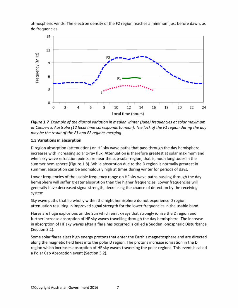
1.4.4 Diurnal variations

At sunrise (at ionospheric heights), EUV radiation produces electrons in the ionosphere, electron

concentration increases sufficiently to enable the E and F1 regions to refract HF sky waves and

higher frequencies to be supported by the F2 region (Figure 1.7).

From sunrise to noon the EUV flux increases, increasing the production of electrons and allowing

higher frequencies to be refracted by all regions. EUV flux peaks around noon leading to the

maximum electron concentration in the ionosphere occurring then or slightly later.

As the afternoon progresses, the EUV flux decreases and the electron density and frequencies

slowly decline.

At sunset, with no EUV radiation to produce electrons, the E and F1 regions essentially become

transparent to HF radio waves as electrons quickly dissipate. The F2 region is sustained through

the night, although with declining electron density, due to the longer lifetimes of electrons and


atmospheric winds. The electron density of the F2 region reaches a minimum just before dawn, as

do frequencies.

Figure 1.7 Example of the diurnal variation in median winter (June) frequencies at solar maximum

at Canberra, Australia (12 local time corresponds to noon). The lack of the F1 region during the day

may be the result of the F1 and F2 regions merging.

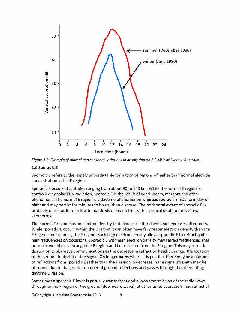
1.5 Variations in absorption

D region absorption (attenuation) on HF sky wave paths that pass through the day hemisphere

increases with increasing solar x-ray flux. Attenuation is therefore greatest at solar maximum and

when sky wave refraction points are near the sub-solar region, that is, noon longitudes in the

summer hemisphere (Figure 1.8). While absorption due to the D region is normally greatest in

summer, absorption can be anomalously high at times during winter for periods of days.

Lower frequencies of the usable frequency range on HF sky wave paths passing through the day

hemisphere will suffer greater absorption than the higher frequencies. Lower frequencies will

generally have decreased signal strength, decreasing the chance of detection by the receiving

system.

Sky wave paths that lie wholly within the night hemisphere do not experience D region

attenuation resulting in improved signal strength for the lower frequencies in the usable band.

Flares are huge explosions on the Sun which emit x-rays that strongly ionise the D region and

further increase absorption of HF sky waves travelling through the day hemisphere. The increase

in absorption of HF sky waves after a flare has occurred is called a Sudden Ionospheric Disturbance

(Section 3.1).

Some solar flares eject high energy protons that enter the Earth's magnetosphere and are directed

along the magnetic field lines into the polar D region. The protons increase ionisation in the D

region which increases absorption of HF sky waves traversing the polar regions. This event is called

a Polar Cap Absorption event (Section 3.2).

0

3

6

9

12

15

Local time (hours)

Fre

qu

en

cy (

MH

z)

0 2 4 6 8 10 12 14 16 18 20 22 24

F2

F1

E


Figure 1.8 Example of diurnal and seasonal variations in absorption on 2.2 MHz at Sydney, Australia.

1.6 Sporadic E

Sporadic E refers to the largely unpredictable formation of regions of higher than normal electron

concentration in the E region.

Sporadic E occurs at altitudes ranging from about 90 to 140 km. While the normal E region is

controlled by solar EUV radiation, sporadic E is the result of wind shears, meteors and other

phenomena. The normal E region is a daytime phenomenon whereas sporadic E may form day or

night and may persist for minutes to hours, then disperse. The horizontal extent of sporadic E is

probably of the order of a few to hundreds of kilometres with a vertical depth of only a few

kilometres.

The normal E region has an electron density that increases after dawn and decreases after noon.

While sporadic E occurs within the E region it can often have far greater electron density than the

E region, and at times, the F region. Such high electron density allows sporadic E to refract quite

high frequencies on occasions. Sporadic E with high electron density may refract frequencies that

normally would pass through the E region and be refracted from the F region. This may result in

disruption to sky wave communications as the decrease in refraction height changes the location

of the ground footprint of the signal. On longer paths where it is possible there may be a number

of refractions from sporadic E rather than the F region, a decrease in the signal strength may be

observed due to the greater number of ground reflections and passes through the attenuating

daytime D region.

Sometimes a sporadic E layer is partially transparent and allows transmission of the radio wave

through to the F region or the ground (downward wave); at other times sporadic E may refract all

summer (December 1980)

winter (June 1980)

Ve

rtic

al

ab

sorp

tio

n (

dB

)

Local time (hours)

50

40

30

20

10

0 2 4 6 8 10 12 14 16 18 20 22 24


the wave energy (from either above or below). A sporadic E layer that is partially transparent may

lead to a weak or fading signal as the layer evolves (Figure 1.9). Transmission to the receiver site

may be blocked completely on oblique paths when the sporadic E screens the F region (wave

travelling up) or the ground (wave returning to ground).

Figure 1.9 Oblique sky wave path with no sporadic E present (dotted red). Sporadic E forms along

the path and its electron density is sufficiently high to refract the wave (solid yellow). On the dotted

red path in the reverse direction, the wave may be refracted from the top of the sporadic E. In the

two latter cases, communications may be disrupted.

Sporadic E formation is more prevalent during the daytime and early evening, and the summer

months at low and middle latitudes. At high latitudes, sporadic E tends to form at night and in

conjunction with a disturbed ionosphere following solar activity.


2. Communications

2.1 HF propagation

High Frequency radio waves can propagate to a distant receiver (Figure 2.1) via the:

• ground wave: near the ground for short distances, up to 100 km over land and 300 km over

sea. Attenuation of the wave depends on antenna height above ground, polarisation,

frequency, ground types, terrain and/or sea state;

• direct or line-of-sight wave: this wave may interact with the earth-reflected wave

depending on terminal separation, frequency and polarisation;

• sky wave: refracted by the ionosphere to all distances.

Figure 2.1 HF frequencies may propagate via the ground wave, line-of-sight, or the sky wave.

2.2 Frequency limits of HF sky waves – the usable frequency range

Not all HF frequencies on a particular sky wave path are refracted back to the ground. Lower

frequencies may be severely attenuated by the D region while higher frequencies may pass

through the ionosphere. The range of usable frequencies will vary:

• diurnally;

• with the seasons;

• with the solar cycle;

• with the location of ionospheric refraction points.

For a particular sky wave path at a particular time, there is a Maximum Observed Frequency (MOF)

that is refracted from the ionosphere back to Earth; this maximum frequency is usually

determined by the electron density of the F region. Frequencies higher than the MOF penetrate

the ionosphere. Over time, the MOF varies because the ionospheric electron concentration and

structure vary.

For a particular sky wave path at a particular time, lower frequencies than the MOF may

propagate. These lower frequencies are generally refracted from lower altitudes in the

ionosphere.

The lowest frequency that can propagate on a sky wave path at a particular time during daytime is

dependent on the ionisation in the D region. Variations in D region ionisation cause this lowest


frequency to change over time. Each time a sky wave traverses the D region, the signal strength

decreases. Furthermore, the signal attenuation due to the D region is greater at lower frequencies.

Sky wave paths that lie completely within the night hemisphere are unaffected by the D region

and may be able to use the lowest frequencies in the HF band.

Ultimately, the lowest frequency detected will be determined by the sensitivity of the receiving

system.

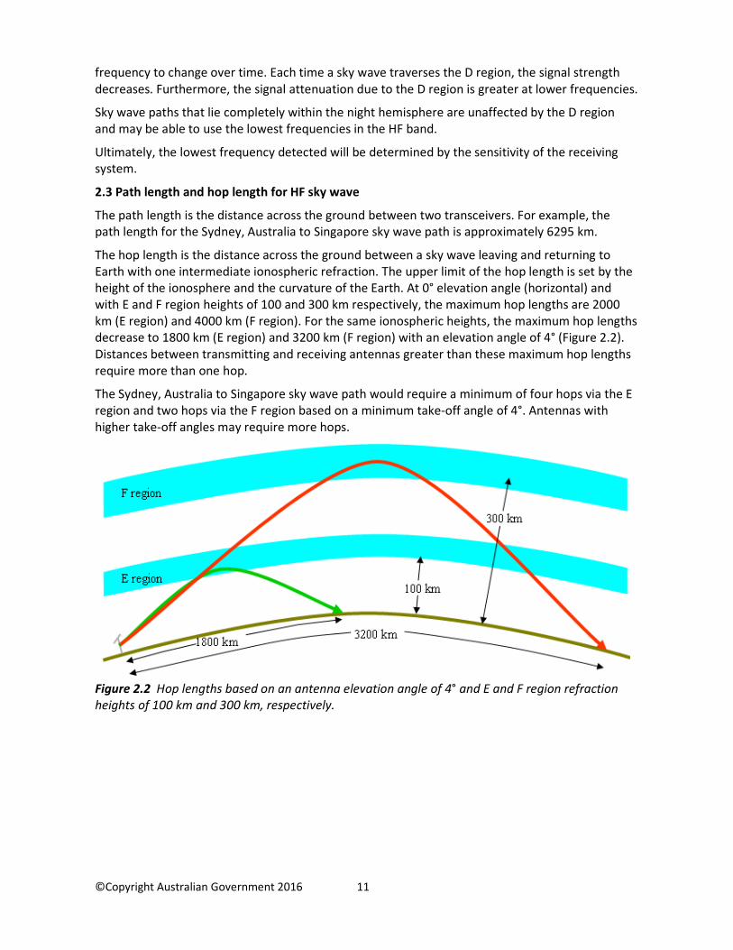
2.3 Path length and hop length for HF sky wave

The path length is the distance across the ground between two transceivers. For example, the

path length for the Sydney, Australia to Singapore sky wave path is approximately 6295 km.

The hop length is the distance across the ground between a sky wave leaving and returning to

Earth with one intermediate ionospheric refraction. The upper limit of the hop length is set by the

height of the ionosphere and the curvature of the Earth. At 0° elevation angle (horizontal) and

with E and F region heights of 100 and 300 km respectively, the maximum hop lengths are 2000

km (E region) and 4000 km (F region). For the same ionospheric heights, the maximum hop lengths

decrease to 1800 km (E region) and 3200 km (F region) with an elevation angle of 4° (Figure 2.2).

Distances between transmitting and receiving antennas greater than these maximum hop lengths

require more than one hop.

The Sydney, Australia to Singapore sky wave path would require a minimum of four hops via the E

region and two hops via the F region based on a minimum take-off angle of 4°. Antennas with

higher take-off angles may require more hops.

Figure 2.2 Hop lengths based on an antenna elevation angle of 4° and E and F region refraction

heights of 100 km and 300 km, respectively.


2.4 Propagation modes of HF sky wave

The HF wave emitted from an antenna may travel via different sky wave paths (modes) between

two ground-based transceivers. These modes are dependent on the gain pattern of the

transmitting antenna, the operating frequency and the state of the ionosphere.

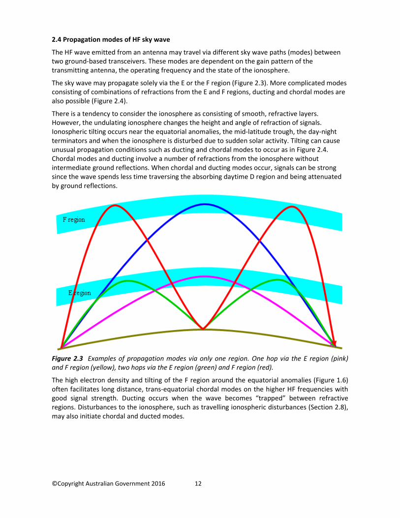
The sky wave may propagate solely via the E or the F region (Figure 2.3). More complicated modes

consisting of combinations of refractions from the E and F regions, ducting and chordal modes are

also possible (Figure 2.4).

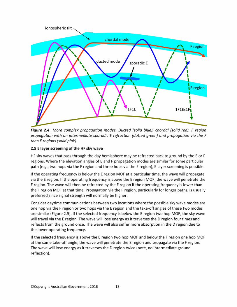
There is a tendency to consider the ionosphere as consisting of smooth, refractive layers.

However, the undulating ionosphere changes the height and angle of refraction of signals.

Ionospheric tilting occurs near the equatorial anomalies, the mid-latitude trough, the day-night

terminators and when the ionosphere is disturbed due to sudden solar activity. Tilting can cause

unusual propagation conditions such as ducting and chordal modes to occur as in Figure 2.4.

Chordal modes and ducting involve a number of refractions from the ionosphere without

intermediate ground reflections. When chordal and ducting modes occur, signals can be strong

since the wave spends less time traversing the absorbing daytime D region and being attenuated

by ground reflections.

Figure 2.3 Examples of propagation modes via only one region. One hop via the E region (pink)

and F region (yellow), two hops via the E region (green) and F region (red).

The high electron density and tilting of the F region around the equatorial anomalies (Figure 1.6)

often facilitates long distance, trans-equatorial chordal modes on the higher HF frequencies with

good signal strength. Ducting occurs when the wave becomes “trapped” between refractive

regions. Disturbances to the ionosphere, such as travelling ionospheric disturbances (Section 2.8),

may also initiate chordal and ducted modes.


Figure 2.4 More complex propagation modes. Ducted (solid blue), chordal (solid red), F region

propagation with an intermediate sporadic E refraction (dotted green) and propagation via the F

then E regions (solid pink).

2.5 E layer screening of the HF sky wave

HF sky waves that pass through the day hemisphere may be refracted back to ground by the E or F

regions. Where the elevation angles of E and F propagation modes are similar for some particular

path (e.g., two hops via the F region and three hops via the E region), E layer screening is possible.

If the operating frequency is below the E region MOF at a particular time, the wave will propagate

via the E region. If the operating frequency is above the E region MOF, the wave will penetrate the

E region. The wave will then be refracted by the F region if the operating frequency is lower than

the F region MOF at that time. Propagation via the F region, particularly for longer paths, is usually

preferred since signal strength will normally be higher.

Consider daytime communications between two locations where the possible sky wave modes are

one hop via the F region or two hops via the E region and the take-off angles of these two modes

are similar (Figure 2.5). If the selected frequency is below the E region two hop MOF, the sky wave

will travel via the E region. The wave will lose energy as it traverses the D region four times and

reflects from the ground once. The wave will also suffer more absorption in the D region due to

the lower operating frequency.

If the selected frequency is above the E region two hop MOF and below the F region one hop MOF

at the same take-off angle, the wave will penetrate the E region and propagate via the F region.

The wave will lose energy as it traverses the D region twice (note, no intermediate ground

reflection).

ducted mode

1F1Es1F

sporadic E

ionospheric tilt

1F1E

E region

F region

chordal mode


The wave may successfully propagate via the E region two hop mode. However, signal strength

may be lower due to higher absorption and ground reflection losses and, depending on the

sensitivity of the receiving system, may not be detected.

Figure 2.5 In this example, E layer screening occurs if communications are intended by the F region

one hop mode but the operating frequency is equal to or below the E region two hop MOF (dotted

green). If the operating frequency is above the E region two hop MOF and less than or equal to the

F region one hop MOF at the same angle, the wave penetrates the E region and refracts from the F

region (solid red) - no E layer screening occurs.

E layer screening can be avoided by ensuring the operating frequency is above the E region MOF in

cases where both E and F region propagation are possible and the modes have similar take-off

angles. SWS ASAPS and GRAFEX predictions calculate a predicted E region MUF (Maximum Usable

Frequency). Selecting a frequency somewhat above the predicted E region MUF should result in an

operating frequency that propagates via the F region.

E region sky wave propagation over distances of less than about 3600 km (two E region hops) can

be successful. It has the advantage of being unaffected by ionospheric storms and has lower day

to day MOF variability at a certain hour. However, the use of the lower frequencies may lead to

lower signal strength and greater chance of disruption from sudden ionospheric disturbances

(Section 3.1).

Sporadic E may also screen a wave from the F region when it develops day or night. It can be more

difficult to deal with due to its unpredictability and variability in the MOF. Its MOF may also be

much higher than the F region MOF. Sporadic E can partially screen the F region leading to a weak

or fading signal while at other times it can totally obscure the F region possibly causing the

receiving antenna to lie outside the sky wave footprint (Figure 1.9 and Section 1.6). Instruments

such as vertical incidence ionosondes for short range sky wave paths or oblique sounders are able

to observe sporadic E occurrence.

1F

2E

F region

E region

operating frequency ≤ 2E MOF

2E MOF > operating frequency ≤ 1F MOF


2.6 Frequency, range and elevation angle

For an HF sky wave path, there are three interdependent variables:

• frequency;

• range or path length;

• antenna elevation angle.

Figures 2.6, 2.7 and 2.8 illustrate the possible ray paths when each of the variables is fixed in turn.

Figure 2.6 (elevation angle fixed):

• as the operating frequency is increased toward the highest frequency an ionospheric region

can refract at a fixed elevation angle (MOF), the wave is refracted from higher in that region

and the path length (ground range) increases (rays 1 and 2);

• when the operating frequency equals the MOF, the maximum path length is achieved (ray

3);

• when the operating frequency is greater than the MOF, the wave penetrates the ionospheric

region (ray 4).

Figure 2.6 Elevation angle fixed. Increasing the frequency increases the path length.

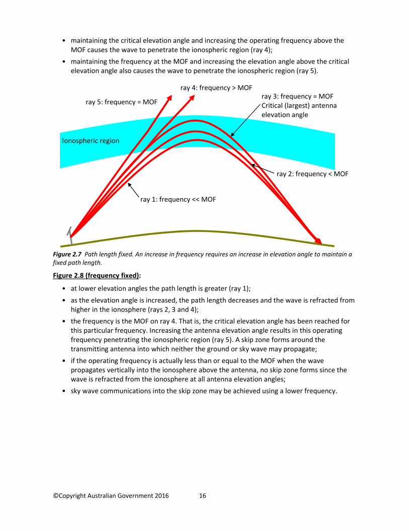
Figure 2.7 (path length fixed):

• as the operating frequency is increased towards the highest frequency an ionospheric region

can refract at some particular antenna elevation angle (MOF), the wave is refracted from

higher in the ionospheric region and returns to the ground at greater distances from the

transmitting antenna (Figure 2.6). To maintain a fixed path length, the elevation angle must

therefore be increased as the frequency increases (Figure 2.7, rays 1 and 2);

• the highest possible operating frequency for a fixed path length using a certain ionospheric

region coincides with the largest antenna elevation angle for this ionospheric region. This is

termed the critical elevation angle (ray 3). The highest frequency that is refracted at the

critical elevation angle for a particular ionospheric region is the MOF;

ray 1: frequency < MOF ray 2:

frequency < MOF

ray 3: frequency = MOF Ionospheric region

ray 4: frequency > MOF


• maintaining the critical elevation angle and increasing the operating frequency above the

MOF causes the wave to penetrate the ionospheric region (ray 4);

• maintaining the frequency at the MOF and increasing the elevation angle above the critical

elevation angle also causes the wave to penetrate the ionospheric region (ray 5).

Figure 2.7 Path length fixed. An increase in frequency requires an increase in elevation angle to maintain a

fixed path length.

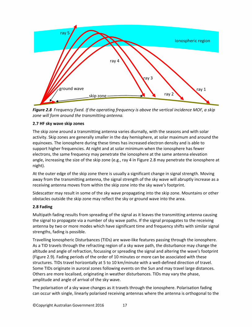
Figure 2.8 (frequency fixed):

• at lower elevation angles the path length is greater (ray 1);

• as the elevation angle is increased, the path length decreases and the wave is refracted from

higher in the ionosphere (rays 2, 3 and 4);

• the frequency is the MOF on ray 4. That is, the critical elevation angle has been reached for

this particular frequency. Increasing the antenna elevation angle results in this operating

frequency penetrating the ionospheric region (ray 5). A skip zone forms around the

transmitting antenna into which neither the ground or sky wave may propagate;

• if the operating frequency is actually less than or equal to the MOF when the wave

propagates vertically into the ionosphere above the antenna, no skip zone forms since the

wave is refracted from the ionosphere at all antenna elevation angles;

• sky wave communications into the skip zone may be achieved using a lower frequency.

ray 1: frequency << MOF

ray 5: frequency = MOF

ray 2: frequency < MOF

ray 3: frequency = MOF

Critical (largest) antenna

elevation angle

Ionospheric region

ray 4: frequency > MOF


Figure 2.8 Frequency fixed. If the operating frequency is above the vertical incidence MOF, a skip

zone will form around the transmitting antenna.

2.7 HF sky wave skip zones

The skip zone around a transmitting antenna varies diurnally, with the seasons and with solar

activity. Skip zones are generally smaller in the day hemisphere, at solar maximum and around the

equinoxes. The ionosphere during these times has increased electron density and is able to

support higher frequencies. At night and at solar minimum when the ionosphere has fewer

electrons, the same frequency may penetrate the ionosphere at the same antenna elevation

angle, increasing the size of the skip zone (e.g., ray 4 in Figure 2.8 may penetrate the ionosphere at

night).

At the outer edge of the skip zone there is usually a significant change in signal strength. Moving

away from the transmitting antenna, the signal strength of the sky wave will abruptly increase as a

receiving antenna moves from within the skip zone into the sky wave's footprint.

Sidescatter may result in some of the sky wave propagating into the skip zone. Mountains or other

obstacles outside the skip zone may reflect the sky or ground wave into the area.

2.8 Fading

Multipath fading results from spreading of the signal as it leaves the transmitting antenna causing

the signal to propagate via a number of sky wave paths. If the signal propagates to the receiving

antenna by two or more modes which have significant time and frequency shifts with similar signal

strengths, fading is possible.

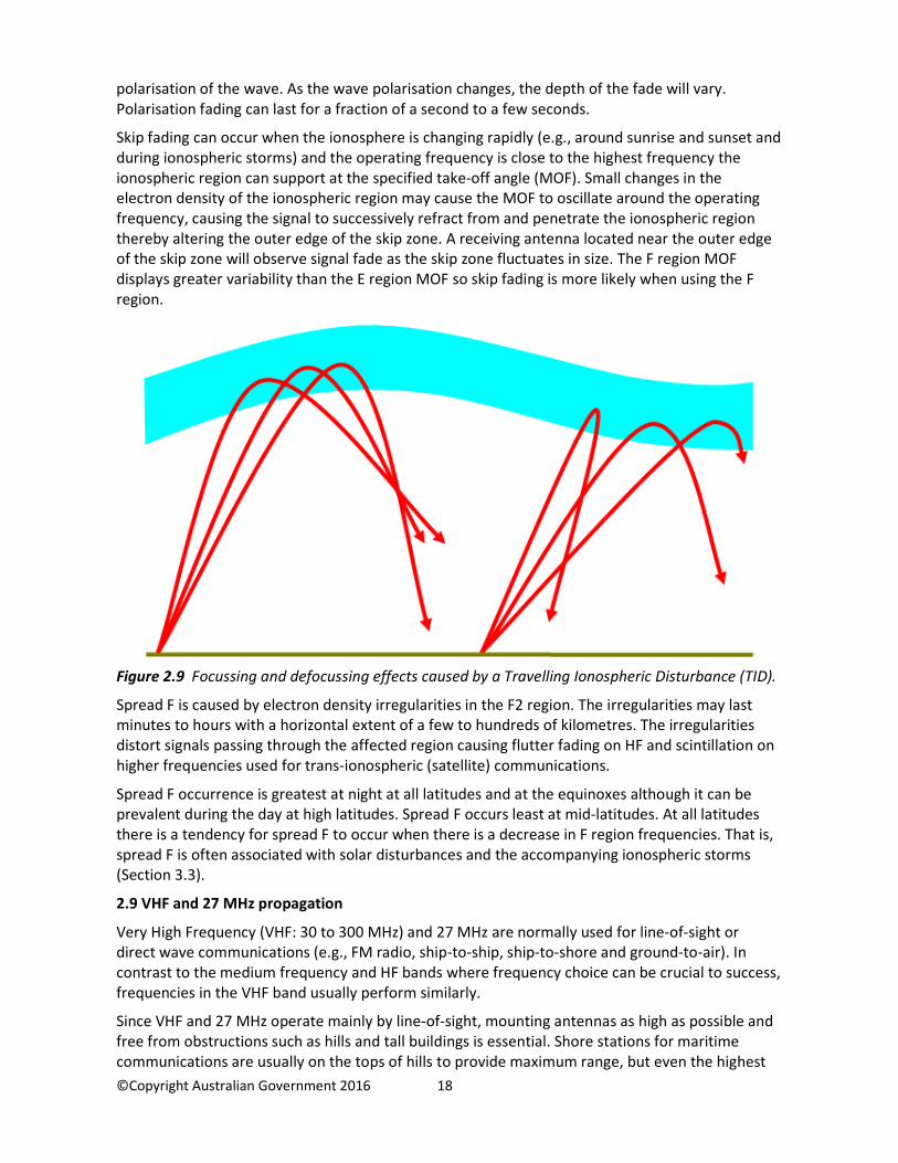
Travelling Ionospheric Disturbances (TIDs) are wave-like features passing through the ionosphere.

As a TID travels through the refracting region of a sky wave path, the disturbance may change the

altitude and angle of refraction, focussing or spreading the signal and altering the wave's footprint

(Figure 2.9). Fading periods of the order of 10 minutes or more can be associated with these

structures. TIDs travel horizontally at 5 to 10 km/minute with a well-defined direction of travel.

Some TIDs originate in auroral zones following events on the Sun and may travel large distances.

Others are more localised, originating in weather disturbances. TIDs may vary the phase,

amplitude and angle of arrival of the sky wave.

The polarisation of a sky wave changes as it travels through the ionosphere. Polarisation fading

can occur with single, linearly polarised receiving antennas where the antenna is orthogonal to the

Ionospheric region

ray 1 ray 2

ray 3

skip zone

ground wave

ray 4

ray 5


polarisation of the wave. As the wave polarisation changes, the depth of the fade will vary.

Polarisation fading can last for a fraction of a second to a few seconds.

Skip fading can occur when the ionosphere is changing rapidly (e.g., around sunrise and sunset and

during ionospheric storms) and the operating frequency is close to the highest frequency the

ionospheric region can support at the specified take-off angle (MOF). Small changes in the

electron density of the ionospheric region may cause the MOF to oscillate around the operating

frequency, causing the signal to successively refract from and penetrate the ionospheric region

thereby altering the outer edge of the skip zone. A receiving antenna located near the outer edge

of the skip zone will observe signal fade as the skip zone fluctuates in size. The F region MOF

displays greater variability than the E region MOF so skip fading is more likely when using the F

region.

Figure 2.9 Focussing and defocussing effects caused by a Travelling Ionospheric Disturbance (TID).

Spread F is caused by electron density irregularities in the F2 region. The irregularities may last

minutes to hours with a horizontal extent of a few to hundreds of kilometres. The irregularities

distort signals passing through the affected region causing flutter fading on HF and scintillation on

higher frequencies used for trans-ionospheric (satellite) communications.

Spread F occurrence is greatest at night at all latitudes and at the equinoxes although it can be

prevalent during the day at high latitudes. Spread F occurs least at mid-latitudes. At all latitudes

there is a tendency for spread F to occur when there is a decrease in F region frequencies. That is,

spread F is often associated with solar disturbances and the accompanying ionospheric storms

(Section 3.3).

2.9 VHF and 27 MHz propagation

Very High Frequency (VHF: 30 to 300 MHz) and 27 MHz are normally used for line-of-sight or

direct wave communications (e.g., FM radio, ship-to-ship, ship-to-shore and ground-to-air). In

contrast to the medium frequency and HF bands where frequency choice can be crucial to success,

frequencies in the VHF band usually perform similarly.

Since VHF and 27 MHz operate mainly by line-of-sight, mounting antennas as high as possible and

free from obstructions such as hills and tall buildings is essential. Shore stations for maritime

communications are usually on the tops of hills to provide maximum range, but even the highest


hills do not provide coverage much beyond about 45 nautical miles (80 km) because of the Earth's

curvature. Antennas for VHF and 27 MHz communications between two ground locations should

concentrate radiation at low angles (towards the horizon).

VHF and 27 MHz do not usually suffer from atmospheric noise effects except during severe

electrical storms. The Sun, man-made noise and galactic noise are the main sources of noise at

VHF. Interference from other users can be a significant problem in densely populated areas.

27 MHz and the lower frequencies in the VHF band can, at times, propagate over large distances,

well beyond the normal line-of-sight limitations. There are three ways this may occur:

• around solar maximum and during the day, the F region will often support long range sky

wave communications on 27 MHz and above as the ionosphere is highly charged;

• electron dense sporadic E can often refract 27 MHz and lower VHF over distances of about

500 to 1000 nautical miles (900 to 1800 km) in length. This is most likely to occur during the

daytime in summer;

• 27 MHz and VHF can also propagate by means of temperature inversions (ducting) at

altitudes of a few kilometres. Under these conditions, the waves are gradually bent by the

temperature inversion to follow the curvature of the Earth. Distances of several hundred

nautical miles can be achieved.

2.10 Medium Frequency sky wave propagation

Sky waves in the Medium Frequency (MF: 300 kHz to 3 MHz) and the lower part of the HF band

normally are highly attenuated by the daytime D region. MF frequencies are restricted to

propagating via the ground wave or line-of-sight in the day hemisphere. The D region is

insignificant at night so that these frequencies can travel large distances via the sky wave in the

night hemisphere. Broadcasts on the AM radio band can often be detected large distances from

the transmitting antenna since there is no absorptive D region then.

2.11 Ground wave MF and HF propagation

It is possible to communicate up to several hundred nautical miles on MF and low HF frequencies

by transmitting the signal across the ground. At these frequencies, the wave follows the curvature

of the Earth.

The range of the ground wave is dependent on the frequency, transmitter power, antenna type,

ground type and terrain.

Lower frequencies suffer fewer losses so have greater range. Greater transmitter power also

increases the range. Ground wave antennas should be normally (vertically) polarised, directing

energy at low angles; vertical whips are appropriate.

The electrical properties of the ground (conductivity and permittivity) decrease with decreasing

moisture content so that a ground wave travelling across sea water is likely to provide the greatest

range while ice will severely restrict the ground wave range.

The signal strength can decrease markedly after the ground wave passes over an obstacle (e.g.

mountain) with the decrease being greater the higher the obstacle. The signal strength tends to

recover somewhat moving away from the obstacle. A receiving antenna located in an obstacle’s

“shadow” will therefore observe a greater reduction in signal strength than perhaps one that is

further from the transmitting antenna but out of the shadow.

The detection of the ground wave varies with the diurnal and seasonal variations in the noise

floor. Signal-to-noise levels will be greatest during the day in winter with noise levels lowest at

these times. Under ideal, low noise conditions, it is possible to communicate over distances of


about 500 nautical miles at 2 MHz using a 100 W transmitter. At 8 MHz under the same conditions

and using the same power, the range is reduced to about 150 nautical miles.

2.12 Noise

Radio noise has internal and external origins. Internal or thermal noise is generated in the

receiving system and is usually negligible when compared to external noise sources in the HF and

lower frequency bands. External radio noise originates from natural (atmospheric and galactic)

and man-made (environmental) sources.

Atmospheric noise, caused by lightning discharges in thunderstorms, is normally the major

contributor to radio noise in the HF band. Thunderstorm occurrence is greatest at low latitudes

and varies seasonally. Atmospheric noise can be impulsive when storms are proximate to the

receiving antenna, or display a broad continuum when storms are remote. This noise may display

some directionality depending on the location and spread of storms with respect to the receiving

antenna. Atmospheric noise effects are greater at lower HF frequencies so are likely to affect

signal quality during the night and solar minimum when lower frequencies are in use.

Galactic noise arises from celestial sources in the Milky Way galaxy and the Sun. Frequencies

above about 15 MHz are mostly affected as the F2 region of the ionosphere screens the lower

frequencies from entering. The higher HF frequencies and receiving antennas with broad gain

patterns are likely to be most affected. Even so, man-made and atmospheric noise will probably

contribute more to noise levels.

Man-made noise results from any large currents and voltages that arise in domestic and industrial

electrical and electronic equipment. Ignition systems, neon signs, electrical cables, power

transmission lines, welding machines, microwave ovens and computers all contribute. The level of

man-made noise depends on the population and technology in use. Interference can be included

in this classification and may be intentional (jamming), due to spurious propagation conditions or

the result of operators ignoring regulations.

A horizontally polarised receiving antenna may alleviate man-made noise since it tends to be

normally polarised (horizontally polarised HF waves travelling across the ground are attenuated

more than normal polarisation).

A narrower bandwidth or a directional receiving antenna will reduce noise levels. Selecting a

receiving antenna site with a low noise floor and determining the major noise sources are

important factors in the establishment of a successful communications system.

2.13 Universal time

Unless transceivers are located within the same time zone, it is appropriate to use Universal Time

(UT) for communication schedules. Universal Time equates to Greenwich Mean Time (GMT) and

Zulu (Z) time. The Universal Time, 0000 UT, occurs at midnight at Greenwich, England.


3. Effects of solar events on HF sky wave communications

Apart from the slowly varying number of sunspots and subsequent change in EUV radiation over a

solar cycle, the Sun can display sudden increases in activity at any time. This sudden activity takes

the form of flares, coronal holes and coronal mass ejections. The consequence to HF sky wave

communications is overlaid on the slowly varying changes due to the solar cycle.

Flares are sudden and massive explosions, usually associated with magnetically complex sunspot

groups. Such sunspot groups are most common around solar maximum. Flares emit energy with a

range of wavelengths, from radio through to gamma.

Coronal holes are the source of high speed solar wind streams which flow out through the solar

wind and can impact the Earth’s magnetosphere. They can endure for months causing recurrent

disturbances in the geomagnetic field and ionosphere.

Coronal mass ejections (CMEs) may occur in conjunction with flares and filament lift offs (the solar

magnetic field reconfigures and material that is suspended in the lower corona is ejected). CMEs

are fast moving bubbles of plasma that speed through the solar wind and can impact the Earth’s

magnetosphere, also disturbing the geomagnetic field and ionosphere.

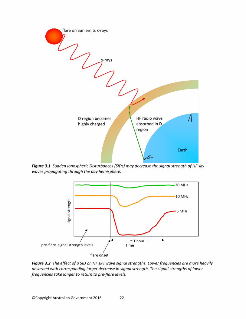
3.1 Sudden Ionospheric Disturbances (SIDs)

Also known as Short Wave Fade-outs (SWFs), the x-ray radiation from the Sun during large solar

flares increases exponentially, enhancing ionisation in the D region which results in greater

absorption of HF sky waves (Figure 3.1). If the flare is large enough, the whole of the HF spectrum

can suffer severe attenuation for a period of time. Large flares and therefore SIDs are more likely

to occur around solar maximum.

The main features of SIDs are:

• only HF sky wave paths that pass through the day hemisphere are affected and those with

refraction points near the sub-solar region are most affected;

• SIDs occur instantaneously with affected frequencies experiencing a sudden decrease in

signal strength;

• the duration of SIDs varies between about 10 minutes to, on rare occasions, several hours

although most are about 20 minutes in length;

• lower frequencies suffer greater reduction in signal strength and take longer to return to

pre-flare levels. Higher frequencies are normally less affected (or unaffected) and may still

be usable (Figure 3.2);

• the intensity of a SID depends on the magnitude and duration of the flare x-ray output, the

location of the ionospheric refraction points in the day hemisphere with respect to the sub-

solar location and the operating frequency.


Figure 3.1 Sudden Ionospheric Disturbances (SIDs) may decrease the signal strength of HF sky

waves propagating through the day hemisphere.

Figure 3.2 The effect of a SID on HF sky wave signal strengths. Lower frequencies are more heavily

absorbed with corresponding larger decrease in signal strength. The signal strengths of lower

frequencies take longer to return to pre-flare levels.

x-rays

flare on Sun emits x-rays

D region becomes

highly charged

Earth

HF radio wave

absorbed in D

region

flare onset

20 MHz

10 MHz

5 MHz

Time ~ 1 hour

sig

na

l st

ren

gth

pre-flare signal strength levels


3.2 Polar Cap Absorption (PCA) events

Some solar flares emit high energy protons as well as x-rays. These fast protons have variable

speeds, some relativistic, arriving at Earth minutes after emission while others may take days to

reach Earth. When the protons enter the Earth's magnetosphere, they are directed along the

magnetic field lines towards the poles. The protons ionise the polar D regions and cause increased

attenuation of HF sky waves that traverse them. PCAs occur most often with larger solar flares

which have a greater likelihood around solar maximum.

The increased attenuation of HF sky waves in the polar regions and subsequent drop in HF signal

strength may commence as soon as a few minutes after the flare onset and persist up to ten days.

PCAs vary in strength over their course due to the temporal variability in protons arriving from the

Sun and entering the D region.

Even the winter polar zone (a region of perpetual darkness) can suffer the effects of PCAs since the

ionised D region is formed by protons rather than the usual x-rays.

The effects of PCAs on polar sky wave paths can sometimes be overcome by relaying messages on

paths which avoid the polar regions. As is usual with D region absorption, the lower frequencies

are likely to be more severely affected.

3.3 Ionospheric storms

Solar events such as coronal holes and coronal mass ejections change the character of the solar

wind, increasing its speed and altering its density and magnetic structure. When the disturbed

solar wind impacts the Earth's magnetosphere, the geomagnetic field and electric fields and

currents at ionospheric altitudes change. The response by the ionosphere, a change in electron

density in the F region, is called an “ionospheric storm”.

Ionospheric storms are characterised by greater than normal variations in the highest frequency

the F region can refract (MOF).

For some HF sky wave paths, the F region MOF increases for a few hours before decreasing below

undisturbed values. On other paths, the MOF simply decreases.

Figure 3.3 shows the behaviour of the F region vertical MOFs above Canberra, Australia over a

four-day period. The ionospheric storm begins in the first half of day two with the MOFs increasing

well above the predicted values. The dramatic decrease in electron density and MOFs occurs on

day three. MOFs are still depressed (below predicted values) on day four.

Disruptions to HF sky wave communications using the F region will occur where the MOF drops

below the operating frequency resulting in the sky wave penetrating the ionosphere.

Communications are likely to be further complicated as the F region becomes turbulent, varying

the refraction altitude and angle and displaying increased variability in the MOF.

Ionospheric storms vary in their behaviour at different locations. They may last a number of days

with high latitudes generally experiencing larger decreases in F region electron density than other

latitudes. The effects of ionospheric storms begin slowly, over hours, have a long duration, a day

to a number of days, and may require the use of lower operating frequencies.

The E region will be mostly unaffected by ionospheric storms.


Figure 3.3 Predicted (dotted red) and observed (solid black) F region vertical MOFs at Canberra,

Australia over four UT days. Noon at 02 UT. Frequencies become enhanced (above predicted

values) around 06 UT on UT day two in response to solar activity. Frequencies are mostly depressed

(below predicted values) on UT days three and four.

0

4

8

12

16

0 6 12 18 0 6 12 18 0 6 12 18 0 6 12 18

Fre

qu

en

cy (

MH

z)

Universal time (hours)

Documents

Space Weather Services - Radio and Space Services