Embed Size (px)
Citation preview
Stefan Dohr, BSc
Space-time boundary element methodsfor the heat equation
MASTERARBEIT
zur Erlangung des akademischen Grades
Diplom-Ingenieur
Masterstudium Technomathematik
eingereicht an der
Technischen Universitat Graz
Betreuer
Prof. Dr. O. Steinbach
Institut fur Numerische Mathematik
Graz, November 2016


Abstract
In this thesis we describe the boundary element method for the discretization of thetime-dependent heat equation. In contrast to standard time-stepping schemes weconsider an arbitrary decomposition of the boundary of the space-time cylinder intoboundary elements. Besides adaptive refinement strategies this approach allows usto parallelize the computation of the global solution of the whole space-time system.In addition to the analysis of the boundary integral operators and the derivation ofboundary element methods for the Dirichlet initial boundary value problem we stateconvergence properties and error estimates of the approximations. Those estimatesare based on the approximation properties of boundary element spaces in anisotropicSobolov spaces, in particular in H
12, 14 (Σ) and H−
12,− 1
4 (Σ). The systems of linear equa-tions, which arise from the discretization of the integral equations, are solved with theGMRES method. For an efficient computation of the solution we need preconditioners.Based on the mapping properties of the single layer- and the hypersingular boundaryintegral operator we construct and analyse a preconditioner for the discretization ofthe first boundary integral equation. Moreover we describe the FEM-BEM couplingmethod for parabolic transmission problems. Finally we present numerical examplesfor the one-dimensional heat equation to confirm the theoretical results.
Kurzfassung
In dieser Arbeit wird die Randelementmethode zur Diskretisierung von zeitabhangigenAnfangsrandwertproblemen am Modell der Warmeleitungsgleichung beschrieben. An-ders als bei klassischen Zeitschrittverfahren wird eine beliebige Zerlegung des Randesdes Raum-Zeit-Zylinders betrachtet, was adaptive Verfeinerungsstrategien und eineParallelisierung des iterativen Losungsverfahrens bezuglich des gesamten Raum-Zeit-Zylinders in einem Schritt ermoglicht. Neben der Analysis der Randintegraloperatorenund der Herleitung von Randelementmethoden fur das Dirichlet-Anfangsrandwertpro-blem werden auch Konvergenzeigenschaften und Fehlerabschatzungen der Naherungslo-sungen angegeben. Diese basieren auf den Approximationseigenschaften von Ansatzrau-men in anisotropen Sobolev-Raumen, insbesondere in H
12, 14 (Σ) bzw. H−
12,− 1
4 (Σ). Dielinearen Gleichungssysteme, welche sich aus der Diskretisierung der Randintegral-gleichungen ergeben, werden mittels GMRES-Verfahren gelost. Fur ein effizientesLosen sind Vorkonditionierer notwendig. Ausgehend von den Abbildungseigenschaftendes Einfachschicht- und des hypersingularen Randintegraloperators und der Projek-tionseigenschaften des Calderon-Operators wird ein Vorkonditionierer fur die Diskreti-sierung der ersten Randintegralgleichung konstruiert und analysiert. Zusatzlich wirddie Methode der FEM-BEM-Kopplung fur parabolische Transmissionsprobleme be-schrieben. Die erarbeiteten theoretischen Aussagen werden anhand von numerischenBeispielen fur die eindimensionale Warmeleitungsgleichung uberpruft.

Vorwort
Die vorliegende Arbeit baut auf meiner Bachelorarbeit und meiner Projektarbeit auf.Seit Beginn meiner Bachelorarbeit beschaftige ich mich mit der Raum-Zeit-Diskre-tisierung der Warmeleitungsgleichung mit der Randelementmethode und mein Inter-esse hierfur ist in den letzten Jahren kontinuierlich gewachsen. Deshalb mochte ichmich in erster Linie bei Univ.-Prof. Dr. O. Steinbach bedanken, der mir dieses Themavorgeschlagen und mich beim Verfassen der Masterarbeit stets unterstutzt hat. Außer-dem mochte ich mich beim gesamten Institut fur Numerische Mathematik der TU Grazfur die Unterstutzung im Studium und die angenehme Atmosphare bedanken.


Contents
Introduction 9
1 Basics 111.1 Operator theory . . . . . . . . . . . . . . . . . . . . . . . . . . . . . . . 111.2 Galerkin methods . . . . . . . . . . . . . . . . . . . . . . . . . . . . . . 12
2 Model problem 152.1 Series representation of the solution . . . . . . . . . . . . . . . . . . . . 15
2.1.1 One-dimensional heat equation . . . . . . . . . . . . . . . . . . 152.1.2 Heat equation in the unit square . . . . . . . . . . . . . . . . . 17
2.2 Representation formula and fundamental solution . . . . . . . . . . . . 18
3 Function spaces 273.1 Standard Sobolev spaces . . . . . . . . . . . . . . . . . . . . . . . . . . 273.2 Anisotropic Sobolev spaces . . . . . . . . . . . . . . . . . . . . . . . . . 293.3 Anisotropic Sobolev spaces on Σ . . . . . . . . . . . . . . . . . . . . . . 303.4 Piecewise smooth functions on Σ . . . . . . . . . . . . . . . . . . . . . 32
4 Existence theorems 35
5 Boundary integral operators 375.1 Initial potential . . . . . . . . . . . . . . . . . . . . . . . . . . . . . . . 375.2 Volume potential . . . . . . . . . . . . . . . . . . . . . . . . . . . . . . 385.3 Single layer potential . . . . . . . . . . . . . . . . . . . . . . . . . . . . 405.4 Adjoint double layer potential . . . . . . . . . . . . . . . . . . . . . . . 415.5 Double layer potential . . . . . . . . . . . . . . . . . . . . . . . . . . . 425.6 Hypersingular boundary integral operator . . . . . . . . . . . . . . . . 44
6 Boundary integral equations 456.1 Ellipticity of the single layer boundary integral operator V . . . . . . . 476.2 Ellipticity of the hypersingular boundary integral operator D . . . . . . 476.3 Steklov-Poincare operator . . . . . . . . . . . . . . . . . . . . . . . . . 486.4 Dirichlet initial boundary value problem . . . . . . . . . . . . . . . . . 49
7 Boundary element methods 537.1 Discretization . . . . . . . . . . . . . . . . . . . . . . . . . . . . . . . . 53
7

8 Contents
7.2 BEM for the Dirichlet initial boundary value problem . . . . . . . . . . 647.3 Error estimates . . . . . . . . . . . . . . . . . . . . . . . . . . . . . . . 65
8 Preconditioning 678.1 Calderon preconditioning . . . . . . . . . . . . . . . . . . . . . . . . . . 67
8.1.1 Piecewise constant basis functions . . . . . . . . . . . . . . . . . 698.1.2 Piecewise linear and continuous basis functions . . . . . . . . . 718.1.3 Dual mesh . . . . . . . . . . . . . . . . . . . . . . . . . . . . . . 72
9 FEM-BEM coupling 759.1 Model problem . . . . . . . . . . . . . . . . . . . . . . . . . . . . . . . 759.2 Coupling . . . . . . . . . . . . . . . . . . . . . . . . . . . . . . . . . . . 769.3 Discretization . . . . . . . . . . . . . . . . . . . . . . . . . . . . . . . . 779.4 Galerkin method . . . . . . . . . . . . . . . . . . . . . . . . . . . . . . 78
10 Numerical examples 8110.1 Preconditioning . . . . . . . . . . . . . . . . . . . . . . . . . . . . . . . 8110.2 FEM-BEM coupling . . . . . . . . . . . . . . . . . . . . . . . . . . . . 87
11 Conclusion and Outlook 91
Bibliography 93

Introduction
In this thesis we describe the boundary element method for the discretization of time-dependent initial boundary value problems using the heat equation as a model problem.There are different numerical methods in order to compute an approximate solutionof time-dependent initial boundary value problems. Besides standard time-steppingschemes [32] and decomposition of the whole space-time domain into finite elements[16] we can use the boundary element method to get an approximation of the solutionof the model problem. As for stationary problems [27] one can use the fundamentalsolution of the partial differential equation and the given boundary and initial condi-tions to derive a representation formula for the solution of the time-dependent modelproblem. The problem is reduced to the boundary and we can apply the trace oper-ators to the representation formula to get boundary integral equations and use somediscretization method to compute an approximate solution of those equations.The presented analysis of the boundary integral operators and boundary integral equa-tions is well established and mainly based on the work of Costabel [2] and Noon [17].There is already a variety of papers regarding different applications of the discretiza-tion of the heat equation with the boundary element method [2, 8, 15, 17, 18, 20]using space-time tensor product spaces to discretize the variational formulations ofthe boundary integral equations. This method refers to a separate triangulation ofthe boundary Γ of the domain Ω and the time interval (0, T ) and uses tensor productspaces as trial spaces. In contrast to this approach we consider an arbitrary decom-position of the boundary Σ of the space-time domain Q = Ω × (0, T ) into boundaryelements. Besides adaptive refinement strategies and in contrast to standard time-stepping schemes this approach allows us to parallelize the computation of the globalsolution of the whole space-time system.In this work we consider a Dirichlet initial boundary value problem for the heat equa-tion. After the derivation of the fundamental solution and the representation formulafor the solution of the model problem we discuss the mapping properties of the heatpotentials and the boundary integral operators, based on [2]. Since Dirichlet boundaryconditions are given, it remains to determine the conormal derivative of the solutionof the model problem. This can be done by solving the boundary integral equations.The analysis of the operators is done in anisotropic Sobolev spaces [12]. In this set-ting the single layer boundary integral operator V and the hypersingular operator Dare not only bounded but also elliptic. Due to the ellipticity of V we can concludeunique solvability of the first boundary integral equation using the standard theory ofelliptic operators [27]. Analoguously we get unique solvability of the integral equation
9

10 Introduction
related to an indirect approach using the single layer potential. After discussing thedifferent approaches of determining the unknown conormal derivative of the solutionwe consider a Galerkin-Bubnov variational formulation in order to discretize the firstboundary integral equation and compute an approximation of the conormal deriva-tive. Our goal is to use an arbitrary triangulation of the boundary of the space-timedomain Q. However, we first consider a separate triangulation of the boundary Γand the time interval (0, T ) and derive approximation properties of the correspondingspace-time tensor product spaces. Afterwards we consider an arbitrary decompositionof the space-time boundary for n = 1, 2 and state approximation properties of thespace of piecewise constant basis functions by using the approximation properties ofthe space-time tensor product spaces. The system of linear equations correspondingto the Galerkin-Bubnov variational formulation is solved with the GMRES method.Since the condition number of the system matrix depends on the mesh size of thetriangulation of the space-time boundary, the iteration number of the iterative solverincreases with each refinement step. To get rid of this dependency we have to applysuitable preconditioning strategies. We present a preconditioning technique using op-erators of opposite order such as V and D. The presented concept is based on [31].An advantage of the boundary element method is the handling of exterior problemsin a natural way. This allows us to apply the FEM-BEM coupling method to trans-mission problems for the heat equation. In Chapter 9 we introduce the concept ofa non-symmetric FEM-BEM coupling method for parabolic transmission problems,based on [24], and use a Galerkin method to compute an approximate solution of theproblem. In the last chapter we present numerical examples for the one-dimensionalheat equation to confirm the theoretical results.
1 Basics
In order to study the unique solvability of boundary integral equations and theirdiscretizations we need some results in operator theory. In this chapter we summarizethe main statements, based on [27].
1.1 Operator theory
Let X be a Hilbert space with norm ‖·‖X =√〈·, ·〉 and X ′ be the dual space of X.
The norm of an element f ∈ X ′ is given by
‖f‖X′ = sup06=v∈X
〈f, v〉‖v‖X
where 〈·, ·〉 denotes the duality pairing on X ′ × X. Let A : X → X ′ be a linear andbounded operator, i.e. there exists a constant cA2 > 0 such that
‖Av‖X′ ≤ cA2 ‖v‖X for all v ∈ X.
We want to find a solution u ∈ X of the operator equation
Au = f (1.1)
where f ∈ X ′ is given. This problem is equivalent to its variational formulation, whichis to find u ∈ X such that
〈Au, v〉 = 〈f, v〉 for all v ∈ X. (1.2)
If the operator A is X-elliptic, i.e. there exists a constant cA1 > 0 such that
〈Av, v〉 ≥ cA1 ‖v‖2X for all v ∈ X,
then the following theorem ensures the unique solvability of the operator equation(1.1).
Theorem 1.1 (Lemma of Lax-Milgram). [27, Theorem 3.2] Let the linear operatorA : X → X ′ be bounded and X-elliptic. For any f ∈ X ′ there exists a unique solutionu ∈ X of the operator equation
Au = f.
The solution u satisfies
‖u‖X ≤1
cA1‖f‖X′ .
11

12 1 Basics
Since (1.2) is equivalent to (1.1) the ellipticity of the operator A ensures the uniquesolvability of the variational formulation of the operator equation as well. Accordingto Theorem 1.1 the inverse operator A−1 : X ′ → X is well defined and satisfies∥∥A−1f
∥∥ ≤ 1
cA1‖f‖X′ for all f ∈ X ′.
Now let us consider a linear and bounded operator B : X → X. For a given g ∈ Xwe want to find a solution of the operator equation
(I −B)u = g. (1.3)
The following theorem ensures unique solvability of equation (1.3) when assuming,that the operator B is a contraction in X, i.e.
‖B‖ = sup06=v∈X
‖Bv‖X‖v‖X
< 1
Theorem 1.2 (Neumann series). [35, Theorem II.1.11] Let X be a Banach-space andlet B : X → X be a linear and bounded operator satisfying ‖B‖ < 1. Then I − B isinvertible and
(I −B)−1 =∞∑k=0
Bk.
The inverse operator satisfies ∥∥(I −B)−1∥∥ ≤ 1
1− ‖B‖.
1.2 Galerkin methods
We want to compute an approximate solution of the variational problem (1.2). Hencewe need unique solvability of the discretized problem as well. Let N ∈ N. We con-sider a finite dimensional subspace Xh := span ϕkNk=1 ⊂ X and want to find anapproximation uh of the solution u of (1.2) where
uh =N∑k=1
ukϕk ∈ Xh. (1.4)
The Galerkin-Bubnov variational formulation is to find uh ∈ Xh such that
〈Auh, vh〉 = 〈f, vh〉 for all vh ∈ Xh. (1.5)
This problem is equivalent to solving the system of linear equations
Ahu = f (1.6)

1.2 Galerkin methods 13
whereAh[l, k] := 〈Aϕk, ϕl〉, f [l] := 〈f, ϕl〉
for l, k = 1, ..., N and u is the vector of coefficients regarding (1.4). For u, v ∈ RN wehave
(Ahu, v) = 〈Auh, vh〉.
Hence we get(Ahv, v) = 〈Avh, vh〉 ≥ cA1 ‖vh‖
2X for all v ∈ RN
which implies the positive definiteness and therefore the invertibility of the matrixAh. Thus, the system of linear equations (1.6) and the variational problem (1.5) areuniquely solvable.Since Xh ⊂ X, we have
〈Au, vh〉 = 〈f, vh〉 for all vh ∈ Xh
where u is the unique solution of the variational problem (1.2). By subtracting (1.5)from this equation we get the Galerkin orthogonality
〈A(u− uh), vh〉 = 0 for all vh ∈ Xh. (1.7)
The following theorem states a stability estimate for the approximate solution uh aswell as an error estimate with respect to the solution u of the variational problem(1.2).
Theorem 1.3 (Cea’s Lemma). [27, Theorem 8.1] Let A : X → X ′ be a bounded andX-elliptic linear operator. For the unique solution uh ∈ Xh of the variational problem(1.5) there holds
‖uh‖X ≤1
cA1‖f‖X′
and
‖u− uh‖X ≤cA2cA1
infvh∈Xh
‖u− vh‖X .
Hence we have quasi-optimality of the Galerkin approximation uh and we can useapproximation properties of the finite dimensional subspace Xh to derive error esti-mates and study the convergence of the Galerkin method.


2 Model problem
Let Ω ⊂ Rn (n = 1, 2, 3) be a bounded domain with Lipschitz-boundary Γ := ∂Ω,T ∈ R with T > 0 and α ∈ R with α > 0. We consider the initial boundary valueproblem
α∂tu(x, t)−∆xu(x, t) = f(x, t) for (x, t) ∈ Q := Ω× (0, T ),
u(x, t) = g(x, t) for (x, t) ∈ Σ := Γ× (0, T ),
u(x, 0) = u0(x) for x ∈ Ω
(2.1)
with given source term f and boundary- and initial conditions g and u0 satisfyingthe compatibility condition g(x, 0) = u0(x) for x ∈ Γ. Our aim is to represent thesolution of the problem in terms of the given data f , g and u0. Before we derivethe representation formula for the solution of the model problem we first considertwo special cases of the heat equation and compute analytical solutions of those twoproblems.
2.1 Series representation of the solution
In this section we derive a series representation of the solution of the homogeneousheat equation with boundary condition g = 0 and initial condition u0. Due to thecompatibility condition we have u0|Γ = 0.
2.1.1 One-dimensional heat equation
Without loss of generality we choose Ω = (0, 1) ⊂ R. Let u0 ∈ C(Ω) be a given initialcondition with u0(0) = u0(1) = 0. We consider the initial boundary value problem
α∂tu(x, t)− ∂xxu(x, t) = 0 for (x, t) ∈ (0, 1)× (0, T ),
u(0, t) = u(1, t) = 0 for t ∈ (0, T ),
u(x, 0) = u0(x) for x ∈ (0, 1).
(2.2)
By using separation of variables, i.e. u(x, t) = X(x)T (t), we get
αX(x)T ′(t) = X ′′(x)T (t)
which is equivalent to
αT ′(t)
T (t)=X ′′(x)
X(x)= λ = const.
15

16 2 Model problem
Together with the boundary conditions in (2.2) we get the Dirichlet eigenvalue problem
X ′′(x)− λX(x) = 0 for x ∈ (0, 1),
X(0) = X(1) = 0(2.3)
and the initial value problem
T ′(t)− 1
αλT (t) = 0 for t > 0,
T (0) = a(2.4)
for some constant a ∈ R. The eigenvalues and eigenfunctions of (2.3) are given by
λk = −(kπ)2
andXk(x) = sin(kπx)
where k ∈ N. The solution of (2.4) is then given by
T (t) = ak exp
(λkt
α
).
We conclude that the functions
uk(x, t) = ak exp
(λkt
α
)sin (kπx)
are solutions of the homogeneous heat equation in (2.2) satisfying the boundary con-ditions uk(0, t) = uk(1, t) = 0. The series representation is given by
u(x, t) =∞∑k=1
ak exp
(−(kπ)2t
α
)sin (kπx).
It remains to determine the coefficients ak ∈ R. Since u has to satisfy the initialcondition we have
u(x, 0) =∞∑k=1
ak sin (kπx)!
= u0(x).
Multiplying the equation with sin (lπx) and integrating over (0, 1) gives
∞∑k=1
ak
∫ 1
0
sin (kπx) sin (lπx)dx =
∫ 1
0
u0(x) sin (lπx)dx.
Since ∫ 1
0
sin (kπx) sin (lπx)dx =
12
if l = k,
0 if l 6= k,
we get
ak = 2
∫ 1
0
u0(x) sin (kπx)dx.

2.1 Series representation of the solution 17
2.1.2 Heat equation in the unit square
Let Ω = (0, 1)×(0, 1) be the unit square and u0 ∈ C(Ω) be some given initial conditionsatisfying the compatibility condition
u0(x, 0) = u0(x, 1) = u0(0, y) = u0(1, y) = 0.
As in the spatially one-dimensional case we use separation of variables , i.e.
u(x, t) = X1(x1)X2(x2)T (t),
to get
αT ′′(t)
T (t)=X ′′1 (x1)
X1(x1)+X ′′2 (x2)
X2(x2)= λ = const.
In consideration of the homogeneous boundary conditions this relation leads to theDirichlet eigenvalue problems
X ′′i (xi)− λiXi(xi) = 0 for xi ∈ (0, 1),
Xi(0) = Xi(1) = 0(2.5)
for i = 1, 2 and the initial value problem
T ′(t)− 1
αλT (t) = 0 for t > 0,
T (0) = a(2.6)
for some constant a ∈ R and λ = λ1 +λ2. The eigenvalues and eigenfunctions of (2.5)are given by
λi,k = −(kπ)2
andXi,k(xi) = sin (kπxi)
where k ∈ N. The solution of (2.6) is then given by
T (t) = akl exp
(λklt
α
)with λkl = − (k2 + l2) π2. Thus, the functions
ukl(x, t) = akl exp
(λklt
α
)sin (kπx1) sin (lπx2)
are solutions of the homogeneous heat equation with boundary condition u|Σ = 0. Thegeneral solution is given by the series
u(x, t) =∞∑k=1
∞∑l=1
akl exp
(−(k2 + l2)π2t
α
)sin (kπx1) sin (lπx2).

18 2 Model problem
It remains to determine the coefficients akl. Similarly to the one-dimensional case weget
akl = 4
∫ 1
0
∫ 1
0
u0(x1, x2) sin (kπx1) sin (lπx2)dx2dx1.
2.2 Representation formula and fundamental
solution
In order to state a solution of the initial boundary value problem (2.1) and to de-rive boundary integral equations the existence of a fundamental solution of the heatequation is essential. In this section we will derive the representation formula for thesolution of the model problem (2.1) including the fundamental solution of the heatequation.
Theorem 2.1 (Green’s first formula). [1, Corollary 7.8] Let Ω ⊂ Rn be a boundeddomain with Lipschitz-boundary Γ = ∂Ω and u ∈ C2(Ω) ∩ C1(Ω). Then there holds∫
Ω
[∆u(x)v(x) +∇u(x) · ∇v(x)] dx =
∫Γ
∂
∂nu(x)v(x)dsx for all v ∈ C1(Ω) ∩ C(Ω).
Assume that u ∈ C2(Q) is a solution of the partial differential equation in (2.1).Multiplying the partial differential equation in (2.1) with a function v ∈ C2(Q) andintegration over Q leads to∫ T
0
∫Ω
[α∂su(y, s)v(y, s)−∆yu(y, s)v(y, s)] dyds =
∫ T
0
∫Ω
f(y, s)v(y, s)dyds.
Applying Theorem 2.1 to the second term of the left hand side gives∫ T
0
∫Ω
[α∂su(y, s)v(y, s) +∇yu(y, s) · ∇yv(y, s)] dyds
=
∫ T
0
∫Ω
f(y, s)v(y, s)dyds+
∫ T
0
∫Γ
∂
∂nyu(y, s)v(y, s)dsyds.
(2.7)
This equation is called Green’s first formula for the heat equation. By using integrationby parts regarding the first term of the left hand side and by rearranging the termswe get
α
∫Ω
u(y, T )v(y, T )dy = α
∫Ω
u(y, 0)v(y, 0)dy +
∫ T
0
∫Ω
f(y, s)v(y, s)dyds
+
∫ T
0
∫Ω
[αu(y, s)∂sv(y, s)−∇yu(y, s) · ∇yv(y, s)] dyds
+
∫ T
0
∫Γ
∂
∂nyu(y, s)v(y, s)dsyds.

2.2 Representation formula and fundamental solution 19
Again, by using Theorem 2.1 we get the equation
α
∫Ω
u(y, T )v(y, T )dy = α
∫Ω
u(y, 0)v(y, 0)dy +
∫ T
0
∫Ω
f(y, s)v(y, s)dyds
−∫ T
0
∫Ω
[−α∂sv(y, s)−∆yv(y, s)]u(y, s)dyds
+
∫ T
0
∫Γ
∂
∂nyu(y, s)v(y, s)dsyds−
∫ T
0
∫Γ
∂
∂nyv(y, s)u(y, s)dsyds.
(2.8)
This equation is called Green’s second formula for the heat equation. We want thethird integral of the right hand side to be zero, i.e. we search for a function v whichis a solution of the adjoint homogeneous heat equation
−α∂sv(y, s)−∆yv(y, s) = 0 for (y, s) ∈ Q.
Since we want to find a representation of the solution u = u(x, t) of the model problem(2.1) we define v as
v(y, s) := U(y − x, t− s)
where (x, t) ∈ Q is fixed. In this case we have
∂sv(y, s) = ∂sU(y − x, t− s) = −∂τU(y − x, τ)
where τ = t− s, thus
α∂τU(y − x, τ)−∆yU(y − x, τ) = 0 for (y, s) ∈ Q.
We assume the function U to be spherically symmetric, i.e. U(y − x, τ) = U(r, τ)where r = |y − x|. For r 6= 0 we get
α∂τ U(r, τ)− ∂rrU(r, τ)− (n− 1)1
r∂rU(r, τ) = 0. (2.9)
With U(r, τ) = τ γg(z), where z =r√τ
, γ ∈ R and τ > 0 (⇔ s < t) we get
∂τ U(r, τ) = γτ γ−1g(z)− 1
2τ γ−1zg′(z),
∂rU(r, τ) = g′(z)τ γ−12 ,
∂rrU(r, τ) = g′′(z)τ γ−1.
Therefore equation (2.9) changes to
α
[γτ γ−1g(z)− 1
2τ γ−1zg′(z)
]− g′′(z)τ γ−1 − (n− 1)
1
rg′(z)τ γ−
12 = 0

20 2 Model problem
which is equivalent to
α
[γg(z)− 1
2zg′(z)
]− g′′(z)− (n− 1)
1
zg′(z) = 0. (2.10)
It remains to solve this ordinary differential equation. First we consider the one-dimensional case n = 1, i.e. we have
αγg(z)− α1
2zg′(z)− g′′(z) = 0
which can be written as
α
(γ +
1
2
)g(z)− d
dz
[α
1
2zg(z) + g′(z)
]= 0.
By choosing γ = −12
we get
d
dz
[α
1
2zg(z) + g′(z)
]= 0.
Hence
α1
2zg(z) + g′(z) = c0
with c0 ∈ R. By setting c0 = 0 and using separation of variables we get
ln g = −α1
4z2 + c1
and with c1 = 0 we conclude
g(z) = exp(−α
4z2)
(2.11)
which is a solution of the differential equation (2.10) for n = 1. When inserting (2.11)into (2.10) for general n we get
0 = α[γ exp
(−α
4z2)
+α
4z2 exp
(−α
4z2)]
+α
2exp
(−α
4z2)
− α2
4z2 exp
(−α
4z2)
+ (n− 1)α
2exp
(−α
4z2)
= exp(−α
4z2)α[γ +
n
2
].
Thus, (2.11) is also a solution in the two- and three dimensional case if γ = −n2.
Reconsidering the definition of the functions U and U we have
U(y − x, t− s) = (t− s)−n/2 exp
(−α|y − x|
2
4(t− s)
)for s < t.
2.2 Representation formula and fundamental solution 21
Due to the singularity of the function U at t = s we consider the space-time-cylinderQt−ε := Ω× (0, t− ε) where 0 < ε < t. Analogously to (2.8) we get
α
∫Ω
u(y, t− ε)v(y, t− ε)dy = α
∫Ω
u(y, 0)v(y, 0)dy +
∫ t−ε
0
∫Ω
f(y, s)v(y, s)dyds
−∫ t−ε
0
∫Ω
[−α∂sv(y, s)−∆yv(y, s)]u(y, s)dyds
+
∫ t−ε
0
∫Γ
∂
∂nyu(y, s)v(y, s)dsyds−
∫ t−ε
0
∫Γ
∂
∂nyv(y, s)u(y, s)dsyds.
With v(y, s) = U(y − x, t− s) we have
α
∫Ω
u(y, t− ε)U(y − x, ε)dy = α
∫Ω
u(y, 0)U(y − x, t)dy
+
∫ t−ε
0
∫Ω
f(y, s)U(y − x, t− s)dyds+
∫ t−ε
0
∫Γ
∂
∂nyu(y, s)U(y − x, t− s)dsyds
−∫ t−ε
0
∫Γ
∂
∂nyU(y − x, t− s)u(y, s)dsyds.
(2.12)Let us consider the integral of the left hand side that is
α
∫Ω
u(y, t− ε)U(y − x, ε)dy = α
∫Ω
ε−n/2u(y, t− ε) exp
(−α|y − x|
2
4ε
)dy.
By using the Taylor expansion u(y, t− ε) = u(x, t) + (y− x)>∇xu(ξx, ξt)− ε∂tu(ξx, ξt)with (
ξxξt
)=
(x+ θ(y − x)
t− θε
)where θ ∈ (0, 1) we get
α
εn/2
∫Ω
u(y, t− ε) exp
(−α|y − x|
2
4ε
)dy = u(x, t)
α
εn/2
∫Ω
exp
(−α|y − x|
2
4ε
)dy
+α
εn/2
∫Ω
(y − x)T∇xu(ξx, ξt) exp
(−α|y − x|
2
4ε
)dy
− α
εn/2−1
∫Ω
∂tu(ξx, ξt) exp
(−α|y − x|
2
4ε
)dy.
(2.13)Next we are going to show the convergence of the first integral of the right hand side.First we consider the spatially one-dimensional case n = 1, i.e. Ω = (a, b) with a, b ∈ R

22 2 Model problem
and x ∈ (a, b). We have
A : =α
ε1/2
∫ b
a
exp
(−α(y − x)2
4ε
)dy
=α
ε1/2
∫ x
a
exp
(−α(y − x)2
4ε
)dy +
α
ε1/2
∫ b
x
exp
(−α(y − x)2
4ε
)dy.
By using the substitution z = x−yx−a for the first integral and z = y−x
b−x for the second onewe get
A =α
ε1/2(x− a)
∫ 1
0
exp
(−α(x− a)2z2
4ε
)dz
+α
ε1/2(b− x)
∫ 1
0
exp
(−α(b− x)2z2
4ε
)dz.
The substitution α(x−a)2z2
4ε= η2 for the first and α(b−x)2z2
4ε= η2 for the second integral
leads to
A = 2√α
(x−a)2
√αε∫
0
exp(−η2
)dη + 2
√α
(b−x)2
√αε∫
0
exp(−η2
)dη
and we finally get
A −→ 4√α
∫ ∞0
exp(−η2
)dη = 2
√απ
as ε → 0. In the two-dimensional case we choose R > 0 such that BR(x) ⊂ Ω andconsider
A :=α
ε
∫BR(x)
exp
(−α|y − x|
2
4ε
)dy.
The integral over Ω \ BR(x) converges to 0, since αε
exp(−α|y−x|2
4ε
)→ 0 for y 6= x as
ε→ 0. By using polar coordinates we get
A =α
ε
∫ R
0
∫ 2π
0
exp
(−αr
2
4ε
)rdϕdr =
2πα
ε
∫ R
0
exp
(−αr
2
4ε
)rdr
= 4π
[1− exp
(−αR
2
4ε
)]−→ 4π
as ε → 0. In the three-dimensional case we also choose R > 0 such that BR(x) ⊂ Ωand consider
A :=α
ε3/2
∫BR(x)
exp
(−α|y − x|
2
4ε
)dy.
As in the two-dimensional case the integral over Ω\BR(x) vanishes. By using sphericalcoordinates we get
A =α
ε3/2
∫ R
0
∫ 2π
0
∫ π
0
exp
(−αr
2
4ε
)r2 sin θdθdϕdr =
4πα
ε3/2
∫ R
0
exp
(−αr
2
4ε
)r2dr.

2.2 Representation formula and fundamental solution 23
The substitution η2 = αr2
4εleads to
A =32π√α
√α4εR∫
0
exp(−η2
)η2dη −→ 32π√
α
∫ ∞0
exp(−η2
)η2dη =
8π3/2
√α
as ε → 0. The other two integrals in (2.13) vanish as ε → 0 due to the boundednessof ∇xu and ∂tu. We finally get the representation formula by taking the limit ε → 0in (2.12), i.e. we have
u(x, t) =
∫Ω
u(y, 0)U?(x− y, t)dy +1
α
∫ t
0
∫Ω
f(y, s)U?(x− y, t− s)dyds
+1
α
∫ t
0
∫Γ
∂
∂nyu(y, s)U?(x− y, t− s)dsyds
− 1
α
∫ t
0
u(y, s)∂
∂nyU?(x− y, t− s)dsyds
(2.14)
where
U?(x− y, t− s) =
(α
4π(t− s)
)n/2exp
(−α|x− y|2
4(t− s)
)for s < t.
The function
U?(x− y, t− s) =
(
α
4π(t− s)
)n/2exp
(−α|x− y|2
4(t− s)
), s < t,
0 , else
(2.15)
is called the fundamental solution of the heat equation. Due to the definition of U?
equation (2.14) can be written as
u(x, t) =
∫Ω
u(y, 0)U?(x− y, t)dy +1
α
∫ T
0
∫Ω
f(y, s)U?(x− y, t− s)dyds
+1
α
∫ T
0
∫Γ
∂
∂nyu(y, s)U?(x− y, t− s)dsyds
− 1
α
∫ T
0
u(y, s)∂
∂nyU?(x− y, t− s)dsyds.
(2.16)
Remark 2.1. Let ε > 0. Due to construction the fundamental solution U? is asolution of the homogeneous heat equation
(α∂t −∆x)U?(x− y, t− s) = 0 for (x, t) ∈ Q and (y, s) ∈ Ω× (0, t− ε).

24 2 Model problem
Moreover the fundamental solution U? defined by (2.15) has the following properties.
Lemma 2.2. For t > 0 there holds∫RnU?(x, t)dx = 1.
Proof. Let t > 0. We have∫RnU?(x, t) =
( α
4πt
)n/2 ∫Rn
exp
(−α|x|2
4t
)dx
= π−n/2∫Rn
exp(−|z|2
)dz
= π−n/2n∏i=1
∫Rn
exp(−z2
i
)dzi = 1.
Lemma 2.3. Let u0 ∈ C(Ω) ∩ L∞(Ω). For x ∈ Ω there holds
limt→0
∫Ω
U?(x− y, t)u0(y)dy = u0(x).
Proof. Let ε > 0 and u0 ∈ C(Ω) ∩ L∞(Ω). The function u0 is defined as
u0(x) =
u0(x) for x ∈ Ω,
0 else.
Due to Lemma 2.2 and since U?(x, t) > 0 for (x, t) ∈ Rn × (0, T ) we have∣∣∣∣∫Ω
U?(x− y, t)u0(y)dy − u0(x)
∣∣∣∣ =
∣∣∣∣∫RnU?(x− y, t)[u0(y)− u0(x)]dy
∣∣∣∣≤∫RnU?(x− y, t) |u0(y)− u0(x)| dy.
Since u0 ist continuous, there exists a constant δ > 0 such that |u0(y)− u0(x)| < ε/2if |y − x| < δ. Hence we can write the last integral as∫
Rn
U?(x− y, t) |u0(y)− u0(x)| dy =
∫Rn\Bδ(x)
U?(x− y, t) |u0(y)− u0(x)| dy
+
∫Bδ(x)
U?(x− y, t) |u0(y)− u0(x)| dy.
2.2 Representation formula and fundamental solution 25
The second integral can be estimated from above by∫Bδ(x)
U?(x− y, t) |u0(y)− u0(x)|︸ ︷︷ ︸<ε/2
dy <ε
2
∫RnU?(x− y, t)dy =
ε
2.
Considering the first integral we have∫Rn\Bδ(x)
U?(x− y, t) |u0(y)− u(x)| dy ≤ 2 ‖u‖L∞(Ω)
∫Rn\Bδ(x)
U?(x− y, t)dy,
since u ∈ L∞(Ω). By using the substitution z = x− y we get∫Rn\Bδ(x)
U?(x− y, t)dy =
∫Rn\Bδ(0)
U?(z, t)dz =( α
4πt
)n/2 ∫Rn\Bδ(0)
exp
(−|z|2α
4t
)dz.
By using polar coordinates we get the estimate∫Rn\Bδ(x)
U?(x− y, t)dy ≤ Ct−n/2∞∫δ
rn−1 exp
(−r2α
4t
)dr = C ′
∞∫at−1/2
ρn−1 exp(−ρ2
)dρ
with suitable constants C,C ′ > 0 and a = δ(α4
)1/2. The last integral converges to zero
as t→ 0, i.e. for t small enough there holds∫Rn\Bδ(x)
U?(x− y, t) |u0(y)− u0(x)| dy < ε/2.
Altogether we have ∣∣∣∣∫Ω
U?(x− y, t)u0(y)dy − u0(x)
∣∣∣∣ < ε
for t small enough. Since ε > 0 was arbitrarily chosen, the assertion is proven.
Due to the representation formula (2.16) it suffices to know the Cauchy data ∂nu|Σand u|Σ to compute the solution of the model problem (2.1). Thus, the problem isreduced to the boundary. Since the boundary datum u|Σ = g is given, it remainsto determine the unknown conormal derivative ∂nu|Σ. By applying the Dirichlet andNeumann trace operators (see Chapter 3) to the representation formula (2.14) we getboundary integral equations, which have to be solved. To study the existence anduniqueness of solutions of the boundary integral equations we have to define suitablefunction spaces, which will be discussed in the following chapter.


3 Function spaces
Solutions of the heat equation show different behaviour in temporal and spatial di-rection. This leads to the concept of anisotropic Sobolev spaces, which we introduceand discuss in this chapter. Under certain conditions we can define trace operatorsacting on those spaces and therefore provide conditions for the given Dirichlet datumg and the unkown Neumann datum ∂nu|Σ of the solution, which result in existence anduniqueness theorems of solutions of the model problem (2.1). The presented resultsare based on [12] and [13].Before introducing the concept of anisotropic Sobolev spaces we recall definitions andproperties of standard Sobolev spaces, based on [14] and [27] .
3.1 Standard Sobolev spaces
Let Ω ⊂ Rn be a bounded domain with boundary Γ := ∂Ω. For k ∈ N0 the Sobolevspace W k
2 (Ω) is defined as
W k2 (Ω) := v ∈ L2(Ω) : Dαv ∈ L2(Ω) for all α ∈ Nn
0 : |α| ≤ k
where Dαv denotes the weak derivative of v of order α [27, Chapter 2.2]. The Sobolevspace W k
2 (Ω) equipped with the scalar product
〈v, w〉Wk2 (Ω) :=
∑|α|≤k
∫Ω
DαvDαw dx
defines a Hilbert space. Let κ ∈ (0, 1) and s := k + κ ∈ R \ N. Then
‖u‖W s2 (Ω) :=
‖u‖2
Wk2 (Ω) + |u|2W s
2 (Ω)
1/2
with
|u|2W s2 (Ω) :=
∑|α|=k
∫Ω
∫Ω
|Dαu(x)−Dαu(y)|2
|x− y|n+2κdxdy
defines a norm called the Sobolev-Slobodeckii norm. The Sobolev space W s2 (Ω) defined
as
W s2 (Ω) :=
v ∈ W k
2 (Ω) : ‖v‖W s2 (Ω) <∞
27
28 3 Function spaces
is a Hilbert space with respect to the scalar product
〈v, w〉W s2 (Ω) := 〈v, w〉Wk
2 (Ω) +∑|α|=k
∫Ω
∫Ω
(Dαv(x)−Dαv(y)) (Dαw(x)−Dαw(y))
|x− y|n+2κdxdy.
The Sobolev spaces Hs(Rn) are introduced using distributions [27, Chapter 2.4]. Thenorm of a function u ∈ Hs(Rn) is given by
‖u‖2Hs(Rn) :=
∫Rn
(1 + |ξ|2
)s |u(ξ)|2 dξ
where u denotes the Fourier transform of u. For s ∈ R+0 we have [27, Theorem 2.4]
Hs(Rn) = W s2 (Rn).
For a domain Ω ⊂ Rn the Sobolev space Hs(Ω) is defined as
Hs(Ω) :=v = v|Ω : v ∈ Hs(Rn)
with norm
‖v‖Hs(Ω) := infv∈Hs(Rn),v|Ω=v
‖v‖Hs(Rn) .
If Ω is a Lipschitz domain we have [27, Theorem 2.6]
Hs(Ω) = W s2 (Ω) for all s > 0.
Moreover we consider the spaces
Hs(Ω) := C∞0 (Ω)‖·‖Hs(Rn) , Hs
0(Ω) := C∞0 (Ω)‖·‖Hs(Ω) .
Again, if Ω is a Lipschitz domain we have [27, Theorem 2.5]
Hs(Ω) =[H−s(Ω)
]′, Hs(Ω) =
[H−s(Ω)
]′for all s ∈ R.
From now on let Ω be a bounded domain with Lipschitz boundary Γ := ∂Ω. Similarlyto what we have seen above we can define Sobolev spaces Hs(Γ) on the boundary Γfor |s| ≤ 1. For s ∈ (0, 1) the Sobolev-Slobodeckii norm is defined as
‖v‖Hs(Γ) :=‖v‖2
L2(Γ) + |v|2Hs(Γ)
1/2
(3.1)
with
|v|2Hs(Γ) =
∫Γ
∫Γ
|v(x)− v(y)|2
|x− y|n−1+2sdsxdsy.

3.2 Anisotropic Sobolev spaces 29
The Sobolev space Hs(Γ) for s ∈ (0, 1) is defined as the completion of C(Γ) withrespect of the Sobolev-Slobodeckii norm (3.1) and is a Hilbert space with scalar product
〈u, v〉Hs(Γ) := 〈u, v〉L2(Γ) +
∫Γ
∫Γ
(u(x)− u(y)) (v(x)− v(y))
|x− y|n−1+2sdxdy.
For s = 0 we have H0(Γ) = L2(Γ).Sobolev spaces with negative order s ∈ (−1, 0) are defined as the dual spaces ofH−s(Γ), i.e. we have
Hs(Γ) :=[H−s(Γ)
]′with norm
‖w‖Hs(Γ) := sup06=v∈H−s(Γ)
〈w, v〉Γ‖v‖H−s(Γ)
where 〈·, ·〉Γ denotes the duality product
〈w, v〉Γ :=
∫Γ
w(x)v(x)dsx.
3.2 Anisotropic Sobolev spaces
In this section we introduce anisotropic Sobolev spaces. The definitions and the mainresults are based on [12] and [13].For r, s ≥ 0 the anisotropic Sobolev space Hr,s(Rn × R) is defined as
Hr,s(Rn × R) := L2(R, Hr(Rn) ∩Hs(R, L2(Rn))
where
v ∈ Hs(R, L2(Rn))⇔(1 + |τ |2
)s/2v ∈ L2(Rn × R)
and v denotes the Fourier transform of v with respect to the time variable t. The spaceL2(R, Hr(Rn)) can be characterized in a similar way by using the Fourier transformwith respect to the spatial variable x. The norm of a function u ∈ Hr,s(Rn × R) isgiven by
‖u‖Hr,s(Rn×R) :=
∫R
∫Rn
[(1 + |ξ|2
)r+(1 + |τ |2
)s] |u(ξ, τ)|2dξdτ.
For Q = Ω × (0, T ), where Ω ⊂ Rn is a bounded Lipschitz domain and T > 0, thespace Hr,s(Q) is defined as the space of restrictions of functions in Hr,s(Rn ×R) to Qequipped with the quotient norm. We write
Hr,s(Q) = L2(0, T ;Hr(Ω)) ∩Hs(0, T ;L2(Ω)).

30 3 Function spaces
Moreover we define the space of functions in Hr,s(Q) with zero initial conditions
Hr,s(Q) :=u = u|Q : u ∈ Hr,s(Ω× (−∞, T )) : u(x, t) = 0 for t < 0
.
Another important space in terms of existence and uniqueness analysis is the space
V(Q) := L2(0, T ;H1(Ω)) ∩H1(0, T ;H−1(Ω))
with norm‖u‖2
V(Q) := ‖u‖2L2(0,T ;H1(Ω)) + ‖α∂tu‖2
L2(0,T ;H−1(Ω)) (3.2)
and its subspaces
V(Q) :=u = u|Q : u ∈ V(Ω× (−∞, T )) : u(x, t) = 0 for t < 0
,
V0(Q) := L2(0, T ;H10 (Ω)) ∩H1(0, T ;H−1(Ω)).
The space V(Q) is the space of functions in V(Q) having zero initial conditions, whereasV0(Q) denotes the space of functions in V(Q) having zero boundary conditions. Thenorms in (3.2) are given by
‖u‖2L2(0,T ;H1(Ω)) :=
∫ T
0
‖u(·, t)‖2H1(Ω) dt
and
‖α∂tu‖2L2(0,T ;H−1(Ω)) := sup
06=v∈L2(0,T ;H10 (Ω))
〈α∂tu, v〉Q‖v‖L2(0,T ;H1
0 (Ω))
with
‖v‖2L2(0,T ;H1
0 (Ω)) :=
∫ T
0
∫Ω
|∇xv(x, t)|2dxdt.
The space V(Q) is a dense subspace of H1, 12 (Q) [12, Theorem 12.4]. An important
property of functions u ∈ V(Q) is, that they are in some sense continuous in time.More precisely we have
u ∈ C([0, T ];L2(Ω)). (3.3)
If u ∈ L2(0, T ;H2(Ω) ∩H1(0, T ;L2(Ω)), then u ∈ C([0, T ];H1(Ω)).
3.3 Anisotropic Sobolev spaces on Σ
The spaces Hr,s(Σ) for r, s ≥ 0 are defined analogously. We have
Hr,s(Σ) := L2(0, T ;Hr(Γ) ∩Hs(0, T ;L2(Γ)).
For r, s ∈ (0, 1) an equivalent norm is given by
‖u‖2Hr,s(Σ) := ‖u‖2
L2(Σ) + |u|2L2(0,T ;Hr(Γ)) + |u|2Hs(0,T ;L2(Γ))
3.3 Anisotropic Sobolev spaces on Σ 31
with
|u|2L2(0,T ;Hr(Γ)) :=
∫ T
0
∫Γ
∫Γ
|u(x, t)− u(y, t)|2
|x− y|n−1+2rdsydsxdt
and
|u|2Hs(0,T ;L2(Γ)) :=
∫ T
0
∫ T
0
‖u(·, t)− u(·, τ)‖2L2(Γ)
|t− τ |1+2sdτdt.
Moreover we define the subspace
Hr,s,0 (Σ) := L2(0, T ;Hr(Γ)) ∩Hs
0(0, T ;L2(Γ))
which is the closure in Hr,s(Σ) of the subspace of functions vanishing in a neighborhoodof t = 0 and t = T . For 0 ≤ s < 1
2we have Hr,s
,0 (Σ) = Hr,s(Σ).Anisotropic Sobolev spaces on Σ with negative order r, s < 0 are defined as the dualspaces of H−r,−s,0 (Σ), i.e. we have
Hr,s(Σ) :=[H−r,−s,0 (Σ)
]′with norm
‖w‖Hr,s(Σ) := sup0 6=v∈H−r,−s,0 (Σ)
〈w, v〉Σ‖v‖H−r,−s(Σ)
where 〈·, ·〉Σ denotes the duality product
〈w, v〉Σ :=
∫Σ
w(y, s)v(y, s)dsyds.
Let Ω ⊂ Rn be a bounded Lipschitz domain with boundary Γ = ∂Ω. For a functionu ∈ C(Q) we define the interior Dirichlet trace
γint0 u(x, t) := lim
Ω3x→x∈Γu(x, t) for (x, t) ∈ Σ.
Hence γint0 u coincides with the restriction of u to the space-time boundary Σ, i.e. we
have γint0 u = u|Σ. The following theorem provides a relation of the Dirichlet trace γint
0 uand u in case of functions in anisotropic Sobolev spaces.
Theorem 3.1. [13, Theorem 2.1] Let u ∈ Hr,s(Q) with r > 12, s ≥ 0. Then there
exists a linear, bounded operator γint0 : Hr,s(Q)→ Hµ,ν(Σ) with∥∥γint0 u∥∥Hµ,ν(Σ)
≤ cT ‖u‖Hr,s(Q) for all u ∈ Hr,s(Q),
where µ = r − 12, ν = s− s
2rand γ0 is an extension of γint0 u = u|Σ for u ∈ C(Q).
If r = 1 and s = 12
we have γint0 : H1, 1
2 (Q)→ H12, 14 (Σ). The Dirichlet trace operator
also satisfies a surjectivity property in the following setting.

32 3 Function spaces
Lemma 3.2. [2, Corollary 2.12] The mapping γint0 : V(Q)→ H12, 14 (Σ) is surjective.
Since we want to compute the conormal derivative of solutions of initial bound-ary value problems, we have to define some Neumann trace operator as well. Letu ∈ C1(Q). The interior Neumann trace of u is defined as
γint1 u(x, t) := lim
Ω3x→x∈Γnx · ∇xu(x, t) for (x, t) ∈ Σ.
Hence γint1 u coincides with the conormal derivative of u, i.e we have γint
1 u = ∂nu|Σ.Again, we want to define the Neumann trace of functions in anisotropic Sobolev spacesas well. Four our purposes it suffices to restrict to the space
H1, 12 (Q,α∂t −∆x) :=
u ∈ H1, 1
2 (Q) : (α∂t −∆)u ∈ L2(Q).
Theorem 3.3. [2, Proposition 2.8] The mapping γint1 : H1, 12 (Q,α∂t−∆x)→ H−
12,− 1
4 (Σ)is linear and bounded. If u ∈ C1(Q) then γint1 u = ∂nu|Σ in the distributional sense.
3.4 Piecewise smooth functions on Σ
Let Γ0 ⊂ Γ = ∂Ω be an open part of the boundary of Ω. For r ≥ 0 we define the space
Hr(Γ0) :=v = v|Γ0 : v ∈ Hr(Γ)
equipped with the quotient norm. For a closed, piecewise smooth boundary Γ =
⋃Ji=1 Γi
with Γi∩Γj = ∅ for i 6= j and r ≥ 0 we define the space of piecewise smooth functionson Γ as
Hrpw(Γ) :=
v ∈ L2(Γ) : v|Γi ∈ Hr(Γi) for i = 1, ..., J
with norm
‖v‖Hrpw(Γ) :=
(J∑i=1
∥∥v|Γi∥∥2
Hr(Γi)
)1/2
.
With Σj := Γj × (0, T ) for j = 1, ..., J we have Σ =⋃Jj=1 Σj. For r ≥ 0 and s ≥ 0 we
define anisotropic Sobolev spaces on the open part Σj of the space-time boundary Σas
Hr,s(Σj) :=v = v|Σj : v ∈ Hr,s(Σ)
,
Hr,s0 (Σj) :=
v = v|Σj : v ∈ Hr,s
,0 (Σ) : supp v ⊂ Σj
and the space of piecewise smooth functions on Σ as
Hr,spw(Σ) :=
v ∈ L2(Σ) : v|Σj ∈ Hr,s(Σj) for j = 1, ..., J

3.4 Piecewise smooth functions on Σ 33
with norm
‖v‖Hr,spw (Σ) :=
(J∑j
∥∥v|Σj∥∥2
Hr,s(Σj)
)1/2
.
For r, s < 0 the anisotropic Sobolev spaces on Σj are defined as the dual spaces
Hr,s(Σj) :=[H−r,−s0 (Σj)
]′, Hr,s(Σj) :=
[H−r,−s(Σj)
]′and
Hr,spw(Σ) :=
J∏j=1
Hr,s(Σj)
with norm
‖w‖Hr,spw (Σ) :=
J∑j=1
∥∥w|Σj∥∥Hr,s(Σj).
Lemma 3.4. For r, s < 0 and w ∈ Hr,spw(Σ) there holds
‖w‖Hr,s(Σ) ≤ ‖w‖Hr,spw (Σ) .
Proof. For w ∈ Hr,spw(Σ) we have
‖w‖Hr,s(Σ) = sup06=v∈H−r,−s,0 (Σ)
|〈w, v〉Σ|‖v‖H−r,−s(Σ)
≤ sup0 6=v∈H−r,−s,0 (Σ)
J∑j=1
|〈w, v〉Σj |‖v‖H−r,−s(Σ)
≤ sup06=v∈H−r,−s,0 (Σ)
J∑j=1
|〈w|Σj , v|Σj〉Σj |∥∥v|Σj∥∥H−r,−s(Σj) .Since H−r,−s,0 (Σ) ⊂ H−r,−s(Σ) we get
‖w‖Hr,s(Σ) ≤ sup06=v∈H−r,−s(Σ)
J∑j=1
|〈w|Σj , v|Σj〉Σj |∥∥v|Σj∥∥H−r,−s(Σj)≤
J∑j=1
sup0 6=vj∈H−r,−s(Σj)
|〈w|Σj , vj〉Σj |‖vj‖H−r,−s(Σj)
= ‖w‖Hr,spw (Σ) .


4 Existence theorems
Using the concept of anisotropic Sobolev spaces we can prove existence and uniquenessof solutions of the initial boundary value problem (2.1). We consider different settingsof the model problem.
Lemma 4.1. [2, Lemma 2.3] Let f ∈ L2(0, T ;H−1(Ω)). Then the initial boundaryvalue problem
α∂tu−∆xu = f in Q,
u = 0 on Σ,
u = 0 on Ω× 0
has a unique solution u ∈ V0(Q).
Theorem 4.2. [5, Chapter 7, Theorem 3]. Let u0 ∈ L2(Ω) and f ∈ L2(Q). Then theinitial boundary value problem
α∂tu−∆xu = f in Q,
u = 0 on Σ,
u = u0 on Ω× 0(4.1)
has a unique solution u ∈ V0(Q).
Regarding the unique solution u ∈ V0(Q) ⊂ H1, 12 (Q) of the initial boundary value
problem (4.1) we have γint0 u ∈ H
12, 14 (Σ) and since (α∂t − ∆x)u = 0 we conclude
u ∈ H1, 12 (Q,α∂t − ∆x) and therefore γint
1 u ∈ H−12,− 1
4 (Σ). Higher regularity of theinitial condition u0 leads to higher regularity of the solution u.
Theorem 4.3. [5, Chapter 7, Theorem 5] Let u0 ∈ H10 (Ω), f ∈ L2(Q) and u ∈ V0(Q)
be the unique solution of problem (4.1). Then u ∈ L2(0, T ;H2(U)) ∩H1(0, T ;L2(U)).
Theorem 4.4. [2, Theorem 2.9] Let g ∈ H 12, 14 (Σ). Then the initial boundary value
problemα∂tu−∆xu = 0 in Q,
u = g on Σ,
u = 0 on Ω× 0(4.2)
has a unique solution u ∈ H1,1/2(Q).
35

36 4 Existence theorems
The unique solution u ∈ H1, 12 (Q) of (4.2) satisfies α∂tu − ∆xu = 0. We conclude
∂tu ∈ L2(0, T ;H−1(Q)), since
∂tu =1
α∆xu ∈ L2(0, T ;H−1(Ω)).
Hence we have u ∈ V(Q).
Theorem 4.5. Let u0 ∈ L2(Ω) and g ∈ H12, 14 (Σ). Then the initial boundary value
problemα∂tu−∆xu = 0 in Q,
u = g on Σ,
u = u0 on Ω× 0(4.3)
has a unique solution u ∈ V(Q).
Proof. Let u ∈ V0(Q) be the unique solution of the initial boundary value problem(4.1) with f = 0 and initial condition u0 ∈ L2(Ω) which exists according to Theorem4.2. For u := u+ u we have
α∂tu−∆xu = 0 in Q,
u = g on Σ,
u = 0 on Ω× 0
since u ∈ C([0, T ], L2(Ω)). Theorem 4.4 implies, that there exists a unique solution
u ∈ V(Q). Hence u = u+ u ∈ V(Q) is a unique solution of (4.3).

5 Boundary integral operators
We consider the Dirichlet initial boundary value problem (2.1) with source term
f ∈ L2(Q), boundary condition g ∈ H 12, 14 (Σ) and initial condition u0 ∈ L2(Ω). The
solution for (x, t) ∈ Q is given by the representation formula
u(x, t) =
∫Ω
U?(x− y, t)u0(y)dy +1
α
∫ T
0
∫Ω
U?(x− y, t− s)f(y, s)dyds
+1
α
∫ T
0
∫Γ
U?(x− y, t− s) ∂
∂nyu(y, s)dsyds
− 1
α
∫ T
0
∫Γ
∂
∂nyU?(x− y, t− s)g(y, s)dsyds.
By applying the trace operators we get boundary integral equations. To study theunique solvability of those equations we have to analyse the mapping properties ofthe heat potentials. The presented theory on boundary integral operators for the heatequation is mainly based on [2].
5.1 Initial potential
Let u0 ∈ L2(Ω). The function
(M0u0)(x, t) :=
∫Ω
U?(x− y, t)u0(y)dy for (x, t) ∈ Q (5.1)
is called initial potential of the heat equation with initial condition u0. For x ∈ Γ andt ∈ (0, T ) we define the boundary integral operators
(M0u0)(x, t) := γint0 (M0u0)(x, t) = lim
Ω3x→x∈Γ(M0u0)(x, t)
and(M1u0)(x, t) := γint
1 (M0u0)(x, t) = limΩ3x→x∈Γ
nx · ∇x(M0u0)(x, t).
The initial potential has the following properties.
Lemma 5.1. The initial potential M0u0 with u0 ∈ L2(Ω) is a solution of the homoge-neous heat equation in Q.
37

38 5 Boundary integral operators
Proof. Let u(x, t) := (M0u0)(x, t) for (x, t) ∈ Q be the intial potential with initialcondition u0 ∈ L2(Ω). We have
α∂tu(x, t)−∆xu(x, t) = (α∂t −∆xu)
∫Ω
U?(x− y, t)u0(y)dy.
The fundamental solution U?(x − y, t) is smooth for t > 0 and x ∈ Ω. Thus, we canexchange integration and differentiation. Using the fact, that U?(x− y, t) is a solutionof the homogeneous heat equation for all y ∈ Ω we get
α∂tu(x, t)−∆xu(x, t) =
∫Ω
[α∂tU?(x− y, t)−∆xU
?(x− y, t)]︸ ︷︷ ︸=0
u0(y)dy = 0.
Lemma 5.2. For u0 ∈ C(Ω) ∩ L∞(Ω) and x ∈ Ω it holds
limt→0
(M0u0)(x, t) = u0(x).
Proof. Follows with Lemma 2.3.
Hence the initial potential satisfies the initial condition.
Lemma 5.3. [18, Lemma 5.4] The mapping M0 : L2(Ω) → H1, 12 (Q,α∂t − ∆x) is
linear and bounded.
Hence according to Lemma 3.1 and Lemma 3.3 the integral operators M0 = γint0 M0
and M1 = γint1 M0 are well defined and bounded. We have
M0 : L2(Ω)→ H12, 14 (Σ),
M1 : L2(Ω)→ H−12,− 1
4 (Σ).
5.2 Volume potential
Let f ∈ L2(Q). The function
(N0f)(x, t) :=1
α
∫ t
0
∫Ω
U?(x− y, t− s)f(y, s)dyds for (x, t) ∈ Q (5.2)
is called volume potential of the heat equation with source term f . For x ∈ Γ andt ∈ (0, T ) we define the boundary integral operators
(N0f)(x, t) := γint0 (N0f)(x, t) = lim
Ω3x→x∈Γ(N0f)(x, t)
and(N1f)(x, t) := γint
1 (N0f)(x, t) = limΩ3x→x∈Γ
nx · ∇x(N0f)(x, t).
5.2 Volume potential 39
Lemma 5.4. Let f ∈ C(Q). The volume potential N0f is a solution of the partialdifferential equation
α∂tu(x, t)−∆xu(x, t) = f(x, t) for (x, t) ∈ Q.
Proof. Let u(x, t) := (N0f)(x, t) for (x, t) ∈ Q be the volume potential with sourceterm f ∈ C(Ω). We have
α∂tu(x, t)−∆xu(x, t) = (α∂t −∆x)(N0f)(x, t)
= (α∂t −∆x) limε→0
1
α
∫ t−ε
0
∫Ω
U?(x− y, t− s)f(y, s)dyds.
Let ε > 0. The fundamental solution U?(x − y, t − s) is smooth for t > 0 ands ∈ (0, t− ε). Hence we can apply the Leibniz integral rule and exchange integrationand differentiation. We have
(α∂t −∆x)1
α
∫ t−ε
0
∫Ω
U?(x− y, t− s)f(y, s)dyds
=
∫ t−ε
0
∫Ω
∂tU?(x− y, t− s)f(y, s)dyds+
∫Ω
U?(x− y, ε)f(y, t− ε)dy
− 1
α
∫ t−ε
0
∫Ω
∆xU?(x− y, t− s)f(y, s)dyds
=
∫ t−ε
0
∫Ω
[∂t −
1
α∆x
]U?(x− y, t− s)f(y, s)dyds
+
∫Ω
U?(x− y, ε)f(y, t− ε)dy.
Since U?(x − y, t − s) is a solution of the homogeneous heat equation for y ∈ Ω ands ∈ (0, t − ε), the first integral of the right hand side vanishes. Additionally Lemma2.3 implies ∫
Ω
U?(x− y, ε)f(y, t− ε)dy −→ f(x, t)
as ε→ 0. Since ε > 0 was arbitrarily chosen we get
(α∂t −∆x)u(x, t) = f(x, t).
By definition the volume potential satisfies (N0f)(x, 0) = 0 for x ∈ Ω. Due to
Lemma 4.1 and Theorem 4.4 we conclude N0 : L2(Ω) → H1, 12 (Q,α∂t − ∆) is linear
and bounded. Hence the integral operators N0 = γint0 N0 and N1 = γint
1 N0 are boundedas well. We have
N0 : L2(Q)→ H12, 14 (Σ),
N1 : L2(Q)→ H−12,− 1
4 (Σ).
40 5 Boundary integral operators
5.3 Single layer potential
The single layer potential of the heat equation with density w ∈ H− 12,− 1
4 (Σ) is definedas
(V w)(x, t) :=1
α
∫ t
0
∫Γ
U?(x− y, t− s)w(y, s)dsyds for (x, t) ∈ Q. (5.3)
For x ∈ Γ and t ∈ (0, T ) we define the single layer boundary integral operator V withdensity w as
(V w)(x, t) := γint0 (V w)(x, t) = lim
Ω3x→x∈Γ(V w)(x, t).
Lemma 5.5. The single layer potential V w with density w is a solution of the homo-geneous heat equation in Q.
Proof. Let (x, t) ∈ Ω× (0, T ) and w ∈ L2(Σ). For u(x, t) := (V w)(x, t) we have
α∂tu(x, t)−∆xu(x, t) = (α∂t −∆x)(V w)(x, t)
= (α∂t −∆x) limε→0
1
α
∫ t−ε
0
∫Γ
U?(x− y, t− s)w(y, s)dsyds.
Let ε > 0. The fundamental solution U?(x − y, t − s) is smooth for y ∈ Ω ands ∈ (0, t − ε). Thus, we can apply the Leibniz integral rule and exchange integrationand differentiation. We have
(α∂t −∆x)1
α
∫ t−ε
0
∫Γ
U?(x− y, t− s)w(y, s)dsyds
=
∫ t−ε
0
∫Γ
∂tU?(x− y, t− s)w(y, s)dsyds+
∫Γ
U?(x− y, ε)w(y, t− ε)dsy
− 1
α
∫ t−ε
0
∫Γ
∆xU?(x− y, t− s)w(y, s)dsyds
=
∫ t−ε
0
∫Γ
[∂t −
1
α∆x
]U?(x− y, t− s)w(y, s)dsyds
+
∫Γ
U?(x− y, ε)w(y, t− ε)dsy
The fundamental solution U?(x − y, t − s) is a solution of the homogeneous heatequation for (x, t) ∈ Ω × (0, T ) and (y, s) ∈ Γ × (0, t − ε). Thus, the first integral ofthe right hand side vanishes. For x ∈ Ω and y ∈ Γ we have x 6= y and therefore thedominated convergence theorem [4, Theorem 5.2] implies∫
Γ
U?(x− y, ε)w(y, t− ε)dsy −→ 0

5.4 Adjoint double layer potential 41
as ε→ 0. Hence we get
(α∂t −∆x)u(x, t) = 0.
By using a density argument we conclude that the statement holds for w ∈ H− 12,− 1
4 (Σ)as well.
Lemma 5.6. [2, Remark 3.2] The mapping V : H−12,− 1
4 (Σ) → H1, 12 (Q,α∂t − ∆x) is
linear and bounded.
Hence V w = γint0 (V w) is well defined and due to Lemma 3.1 the single layer bound-
ary integral operator
V := γint0 V : H−
12,− 1
4 (Σ)→ H12, 14 (Σ)
is linear and bounded, i.e. there exsists a constant cV2 > 0 such that
‖V w‖H
12 ,
14 (Σ)≤ cV2 ‖w‖H− 1
2 ,−14 (Σ)
for all w ∈ H−12,− 1
4 (Σ).
For the exterior trace we have
(V w)(x, t) = γext0 (V w)(x, t) = lim
Rn\Ω3x→x∈Γ(V w)(x, t) for (x, t) ∈ Σ
and therefore we obtain the jump relation[γ0V w
]|Σ
= γext0 (V w)(x, t)− γint
0 (V w)(x, t) = 0 for (x, t) ∈ Σ. (5.4)
5.4 Adjoint double layer potential
Due to Lemma 3.3 the operator γint1 V : H−
12,− 1
4 (Σ) → H−12,− 1
4 (Σ) is linear andbounded.
Lemma 5.7. [7, Chapter 5, Theorem 1]. Let w ∈ C(Σ) and (x, t) ∈ Σ = Γ× (0, T ).
The single layer potential V w satisfies the relation
γint1 (V w)(x, t) = limΩ3x→x∈Γ
nx · ∇x(V w)(x, t) =1
2w(x, t) + (K ′w)(x, t)
where
(K ′w)(x, t) =1
α
∫ t
0
∫Γ
∂
∂nxU?(x− y, t− s)w(y, s)dsyds for (x, t) ∈ Σ
is called the adjoint double layer potential with density w.

42 5 Boundary integral operators
The exterior conormal derivative of the single layer potential satisfies
γext1 (V w)(x, t) = lim
Rn\Ω3x→x∈Γnx · ∇x(V w)(x, t) = −1
2w(x, t) + (K ′w)(x, t).
Thus, we get the jump relation[γ1V w
]|Σ
= γext1 (V w)(x, t)− γint
1 (V w)(x, t) = −w(x, t) for (x, t) ∈ Σ.
Using this relation, we can define the adjoint double boundary integral operator forfunctions w ∈ H− 1
2,− 1
4 (Σ) as
K ′w :=1
2
(γint
1 (V w) + γext1 (V w)
).
Due to the linearity and boundedness of V and the Neumann trace operators themapping
K ′ : H−12,− 1
4 (Σ)→ H−12,− 1
4 (Σ)
is linear and bounded. The jump relation for the conormal derivative of the singlelayer potential holds for functions w ∈ H− 1
2,− 1
4 (Σ) as well, i.e. we have[γ1V w
]|Σ
= −w(x, t) for (x, t) ∈ Σ. (5.5)
5.5 Double layer potential
The double layer potential of the heat equation with density v ∈ H 12, 14 (Σ) is defined
as
(Wv)(x, t) :=1
α
∫ T
0
∫Γ
∂
∂nyU?(x− y, t− s)v(y, s)dsyds for (x, t) ∈ Q. (5.6)
Lemma 5.8. The double layer potential Wv with density v is a solution of the homo-geneous heat equation in Q.
Proof. Let (x, t) ∈ Ω× (0, T ) and v ∈ H 12, 14 (Σ). For u(x, t) := (Wv)(x, t) we have
α∂tu(x, t)−∆xu(x, t) = (α∂t −∆x)(Wv)(x, t)
= (α∂t −∆x) limε→0
1
α
∫ t−ε
0
∫Γ
∂
∂nyU?(x− y, t− s)v(y, s)dsyds.

5.5 Double layer potential 43
Let ε > 0. As in the case of the single layer potential we can apply the Leibniz integralrule and exchange integration and differentiation. We get
(α∂t −∆x)1
α
∫ t−ε
0
∫Γ
∂
∂nyU?(x− y, t− s)v(y, s)dsyds
=
∫ t−ε
0
∫Γ
∂
∂ny
[∂t −
1
α∆x
]U?(x− y, t− s)v(y, s)dsyds
+
∫Γ
∂
∂nyU?(x− y, ε)v(y, t− ε)dsy.
The first integral of the right hand side vanishes, since U?(x − y, t − s) is a solutionof the homogeneous heat equation. For x ∈ Ω and y ∈ Γ we have x 6= y and thereforethe dominated convergence theorem [4, Theorem 5.2] implies∫
Γ
∂
∂nyU?(x− y, ε)v(y, t− ε)dsy −→ 0
as ε→ 0. Hence we have(α∂t −∆x)u(x, t) = 0.
Lemma 5.9. [2, Proposition 3.3] The mapping W : H12, 14 (Σ)→ H1, 1
2 (Q,α∂t−∆x) islinear and bounded.
Thus, the linear operator γint0 W : H
12, 14 (Σ)→ H
12, 14 (Σ) is well defined and bounded.
Lemma 5.10. [7, Chapter 5] Let v ∈ C(Σ) and (x, t) ∈ Σ. The double layer potentialWv satisfies the relation
γint0 (Wv)(x, t) = limΩ3x→x∈Γ
(Wv)(x, t) = −1
2v(x, t) + (Kv)(x, t)
where K denotes the double layer boundary integral operator defined as
(Kv)(x, t) =1
α
∫ T
0
∫Γ
∂
∂nyU?(x− y, t− s)v(y, s)dsyds for (x, t) ∈ Σ.
The exterior Dirichlet trace of the double layer potential satisfies
γext0 (Wv)(x, t) = lim
Rn\Ω3x→x∈Γ(Wv)(x, t) =
1
2v(x, t) + (Kv)(x, t) for (x, t) ∈ Σ.
Hence we have the following jump relation for the Dirichlet trace of the double layerpotential
[γ0Wv]|Σ = γext0 (Wv)(x, t)− γint
0 (Wv)(x, t) = v(x, t) for (x, t) ∈ Σ. (5.7)

44 5 Boundary integral operators
Using this relation we can define the double layer boundary integral operator K forfunctions v ∈ H 1
2, 14 (Σ) as
Kv :=1
2
(γint
0 (Wv) + γext0 (Wv)
).
The boundedness of the mapping
K : H12, 14 (Σ)→ H
12, 14 (Σ)
follows from the boundedness of the operator W and the Dirichlet trace operators.The jump relation (5.7) holds for functions v ∈ H 1
2, 14 (Σ) as well, i.e. we have
[γ0Wv]|Σ = v(x, t) for (x, t) ∈ Σ. (5.8)
5.6 Hypersingular boundary integral operator
The hypersingular operator D with density v ∈ H 12, 14 (Σ) is defined as
(Dv)(x, t) := −γint1 (Wv)(x, t) = − lim
Ω3x→x∈Γnx · ∇x(Wv)(x, t) for (x, t) ∈ Σ.
Due to the boundedness of the operator W and the Neumann trace operator thehypersingular operator
D : H12, 14 (Σ)→ H−
12,− 1
4 (Σ)
is bounded as well, i.e. there exists a constant cD2 > 0 such that
‖Dv‖H−
12 ,−
14 (Σ)≤ cD2 ‖v‖H 1
2 ,14 (Σ)
for all v ∈ H12, 14 (Σ).
The conormal derivative of the double layer potential satisfies the jump relation [2,Theorem 3.4]
[γ1Wv]|Σ = γext1 (Wv)(x, t)− γint
0 (Wv)(x, t) = 0 for (x, t) ∈ Σ.

6 Boundary integral equations
Let us consider the representation formula (2.16) for the solution of the model problem(2.1). For (x, t) ∈ Q we have
u(x, t) = (V γint1 u)(x, t)− (Wγint
0 u)(x, t) + (M0u0)(x, t) + (N0f)(x, t).
By applying the Dirichlet trace operator and recalling the jump relations of the heatpotentials we get the first boundary integral equation
γint0 u(x, t) =(V γint
1 u)(x, t) +1
2γint
0 u(x, t)− (Kγint0 u)(x, t)
+ (M0u0)(x, t) + (N0f)(x, t)(6.1)
for (x, t) ∈ Σ. Similarly by applying the Neumann trace operator we get the secondboundary integral equation
γint1 u(x, t) =
1
2γint
1 u(x, t) + (K ′γint1 u)(x, t) + (Dγint
0 u)(x, t)
+ (M1u0)(x, t) + (N1f)(x, t)(6.2)
for (x, t) ∈ Σ. Together these equations lead to the Calderon system of boundaryintegral equations. We have(
γint0 uγint
1 u
)=
(12I −K VD 1
2I +K ′
)︸ ︷︷ ︸
=: C
(γint
0 uγint
1 u
)+
(M0u0
M1u0
)+
(N0fN1f
).
(6.3)
The operator C is called the Calderon projection operator.
Lemma 6.1. C is a projection, i.e. C = C2.
Proof. Let (ψ, ϕ) ∈ H− 12,− 1
4 (Σ)×H 12, 14 (Σ). Then the function
u(x, t) := (V ψ)(x, t)− (Wϕ)(x, t) for (x, t) ∈ Q
is a solution of the homogeneous heat equation. By applying the trace operators weget the boundary integral equations
γint0 u = V ψ +
(1
2I −K
)ϕ
γint1 u =
(1
2I +K ′
)ψ +Dϕ.
(6.4)
45

46 6 Boundary integral equations
Additionally u is a solution of the homogeneous heat equation with Cauchy dataγint
0 u, γint1 u and inital condition u0 = 0, i.e. we have(
γint0 uγint
1 u
)=
(12I −K VD 1
2I +K ′
)(γint
0 uγint
1 u
).
Inserting (6.4) leads to(12I −K VD 1
2I +K ′
)(ψϕ
)=
(12I −K VD 1
2I +K ′
)2(ψϕ
).
Since the functions ψ, ϕ were arbitrarily chosen, we conclude C = C2.
In consequence of the projection property of the Calderon operator we have thefollowing relations.
Corollary 6.2. The boundary integral operators satisfy
V D =
(1
2I −K
)(1
2I +K
),
DV =
(1
2I +K ′
)(1
2I −K ′
),
V K ′ = KV,
K ′D = DK.
Proof. Follows from C = C2.
Let us recall the mapping properties of the boundary integral operators. We have
V : H−12,− 1
4 (Σ)→ H12, 14 (Σ),
K : H12, 14 (Σ)→ H
12, 14 (Σ),
K ′ : H−12,− 1
4 (Σ)→ H−12,− 1
4 (Σ),
D : H12, 14 (Σ)→ H−
12,− 1
4 (Σ).
(6.5)
Theorem 6.3. [2, Corollary 3.10, Theorem 3.11] The operator
A : H12, 14 (Σ)×H−
12,− 1
4 (Σ)→ H12, 14 (Σ)×H−
12,− 1
4 (Σ)
defined as
A :=
(−K VD K ′
)is an isomorphism and there exists a constant c1 > 0 such that
〈(ψϕ
),
(V −KK ′ D
)(ψϕ
)〉 ≥ c1
(‖ψ‖2
H−12 ,−
14 (Σ)
+ ‖ϕ‖2
H12 ,
14 (Σ)
)for all (ψ, ϕ) ∈ H− 1
2,− 1
4 (Σ)×H 12, 14 (Σ).
By using this theorem we can prove the ellipticity of the operators V and D.
6.1 Ellipticity of the single layer boundary integral operator V 47
6.1 Ellipticity of the single layer boundary integral
operator V
Lemma 6.4. The single layer boundary integral operator V defines an isomorphismand there exists a constant cV1 > 0 such that
〈V w,w〉 ≥ cV1 ‖w‖2
H−12,− 1
4 (Σ)for all w ∈ H−
12,− 1
4 (Σ).
Proof. Follows from Theorem 6.3 with ϕ = 0.
Hence the single layer boundary integral operator V : H−12,− 1
4 (Σ) → H12, 14 (Σ) is
bounded and H−12,− 1
4 (Σ)-elliptic and therefore invertible. Thus, the inverse operator
V −1 : H12, 14 (Σ)→ H−
12,− 1
4 (Σ) is well defined and bounded according to the Lemma ofLax-Milgram (Theorem 1.1). We have
∥∥V −1v∥∥H−
12 ,−
14 (Σ)≤ 1
cV1‖v‖
H12 ,
14 (Σ)
for all v ∈ H12, 14 (Σ).
6.2 Ellipticity of the hypersingular boundary
integral operator D
Lemma 6.5. The hypersingular boundary integral operator D defines an isomorphismand there exists a constant cD1 > 0 such that
〈Dv, v〉 ≥ cD1 ‖v‖2
H12, 14 (Σ)
for all v ∈ H12, 14 (Σ).
Proof. Follows from Theorem 6.3 with ψ = 0.
Hence D is invertible and according to the Lemma of Lax-Milgram (Theorem 1.1)we have ∥∥D−1w
∥∥H
12 ,
14 (Σ)≤ 1
cD1‖w‖
H−12 ,−
14 (Σ)
for all w ∈ H−12,− 1
4 (Σ).
According to Corollary 6.2 we have the relations
V D =
(1
2I −K
)(1
2I +K
),
DV =
(1
2I +K ′
)(1
2I −K ′
).
48 6 Boundary integral equations
Since V and D define isomorphisms, the operators
1
2I −K, 1
2I +K : H
12, 14 (Σ)→ H
12, 14 (Σ),
1
2I −K ′, 1
2I +K ′ : H−
12,− 1
4 (Σ)→ H−12,− 1
4 (Σ)
define isomorphisms as well. Hence these operators are invertible. It is well knownthat under certain circumstances these operators define contractions, see [17] and [19].For example if the boundary Γ is C2, then the double layer boundary integral operatorK defines a contraction for sufficiently small T .
6.3 Steklov-Poincare operator
We consider the system of boundary integral equations corresponding to the homoge-neous heat equation with initial condition u0 = 0. We have(
γint0 uγint
1 u
)=
(12I −K VD 1
2I +K ′
)(γint
0 uγint
1 u
).
Using the first integral equation we can define the Dirichlet to Neumann map
γint1 u = V −1
(1
2I +K
)γint
0 u. (6.6)
The operator
S := V −1
(1
2I +K
): H
12, 14 (Σ)→ H−
12,− 1
4 (Σ) (6.7)
is called Steklov-Poincare operator for the heat equation. When inserting (6.6) intothe second boundary integral equation we obtain
γint1 u =
[D +
(1
2I +K ′
)V −1
(1
2I +K
)]γint
0 u.
Hence we get a symmetric representation of the Steklov-Poincare operator. We have
S = D +
(1
2I +K ′
)V −1
(1
2I +K
). (6.8)
Due to the boundedness of the operators K,K ′, D and V −1 the operator S is boundedas well.
Lemma 6.6. The Steklov-Poincare operator S is H12, 14 (Σ)-elliptic, i.e. there exists a
constant cS1 > 0 such that
〈Sv, v〉 ≥ cS1 ‖v‖2
H12 ,
14 (Σ)
for all v ∈ H12, 14 (Σ).

6.4 Dirichlet initial boundary value problem 49
Proof. For v ∈ H 12, 14 (Σ) we define ψ := V −1
(12I +K
)v ∈ H− 1
2,− 1
4 (Σ) and get
〈(ψv
),
(V −KK ′ D
)(ψv
)〉 =
1
2〈V −1
(1
2I +K
)v, v〉+ 〈v,K ′V −1
(1
2I +K
)v +Dv〉
= 〈v,(
1
2I +K ′
)V −1
(1
2I +K
)v +Dv〉
= 〈v, Sv〉.
The statement follows with Theorem 6.3.
6.4 Dirichlet initial boundary value problem
Let us consider the initial boundary value problem
α∂tu(x, t)−∆xu(x, t) = 0 for (x, t) ∈ Q = Ω× (0, T ),
u(x, t) = g(x, t) for (x, t) ∈ Σ = Γ× (0, T ),
u(x, 0) = u0(x) for x ∈ Ω
with boundary condition g ∈ H12, 14 (Σ) and intial condition u0 ∈ L2(Ω). Then the
solution is given by the representation formula
u(x, t) = (V γint1 u)(x, t)− (Wg)(x, t) + (M0u0)(x, t) for (x, t) ∈ Q.
It remains to determine the unknown conormal derivative γint1 u ∈ H− 1
2, 14 (Σ). There
are different ways to accomplish this. For example we can use the boundary integralequations (6.3) to solve the problem. This is called direct approach. First let usconsider the boundary integral equation (6.1), i.e. we have
γint0 u(x, t) = (V γint
1 u)(x, t) +1
2γint
0 u(x, t)− (Kγint0 u)(x, t) + (M0u0)(x, t)
for (x, t) ∈ Σ. We have to find γint1 u ∈ H− 1
2,− 1
4 (Σ) such that
V γint1 u =
(1
2I +K
)g −M0u0 on Σ.
Since the boundary integral operatorsK : H12, 14 (Σ)→ H
12, 14 (Σ), M0 : L2(Σ)→ H
12, 14 (Σ)
and V : H−12,− 1
4 (Σ) → H12, 14 (Σ) are bounded and V is H−
12,− 1
4 (Σ)-elliptic, there ex-
ists a unique solution γint1 u ∈ H−
12,− 1
4 (Σ) according to the Lemma of Lax-Milgram(Theorem 1.1). The solution γint
1 u satisfies
∥∥γint1 u∥∥H−
12 ,−
14 (Σ)≤ 1
cV1
(∥∥∥∥(1
2I +K
)g
∥∥∥∥H
12 ,
14 (Σ)
+ ‖M0u0‖H 12 ,
14 (Σ)
)≤ 1
cV1
(cW2 ‖g‖H 1
2 ,14 (Σ)
+ cM02 ‖u0‖L2
).

50 6 Boundary integral equations
The variational formulation of the problem is to find γint1 u ∈ H− 1
2,− 1
4 (Σ) such that
〈V γint1 u, τ〉Σ = 〈
(1
2I +K
)g, τ〉Σ − 〈M0u0, τ〉Σ for all τ ∈ H−
12,− 1
4 (Σ).
We could also use the second boundary integral equation to determine the unknownNeumann datum γint
1 u, which is given by
γint1 u(x, t) =
1
2γint
1 u(x, t) + (K ′γint1 u)(x, t) + (Dγint
0 u)(x, t) + (M1u0)(x, t)
for (x, t) ∈ Σ. We have to find γint1 u ∈ H− 1
2,− 1
4 (Σ) such that(1
2I −K ′
)γint
1 u = Dg +M1u0 on Σ.
The operator 12I −K ′ is invertible and therefore there exists a unique solution of the
problem.Another approach is using an indirect formulation with the single layer potential V .A solution of the homogeneous heat equation with initial condition u0 is given by
u(x, t) = (V w)(x, t) + (M0u0)(x, t) for (x, t) ∈ Q
with density w ∈ H− 12,− 1
4 (Σ). By applying the Dirichlet trace operator to this equationwe get
g(x, t) = (V w)(x, t) + (M0u0)(x, t) for (x, t) ∈ Σ. (6.9)
Thus, we have to find w ∈ H− 12,− 1
4 (Σ) such that
V w = g −M0u0 on Σ.
As in the case of the direct formulation with the first boundary integral equationthe unique solvability follows with the Lemma of Lax-Milgram (Theorem 1.1). The
variational formulation is to find w ∈ H− 12,− 1
4 (Σ) such that
〈V w, τ〉Σ = 〈g −M0u0, τ〉Σ for all τ ∈ H−12,− 1
4 (Σ).
In the same way we can use the double layer potential W . The function
u(x, t) = −(Wv)(x, t) + (M0u0)(x, t) for (x, t) ∈ Q
with density v ∈ H 12, 14 (Σ) solves the homogeneous heat equation with initial condition
u0. Applying the Dirichlet trace operator leads to the boundary integral equation
g(x, t) =1
2v(x, t)− (Kv)(x, t) + (M0u0)(x, t) for (x, t) ∈ Σ.

6.4 Dirichlet initial boundary value problem 51
Hence we have to find v ∈ H 12, 14 (Σ) such that(
1
2I −K
)v = g −M0u0 on Σ.
Again, this problem is uniquely solvable since the operator 12I −K is invertible. The
variational formulation of this problem is to find v ∈ H 12, 14 (Σ) such that
〈(
1
2I −K
)v, τ〉Σ = 〈g −M0u0, τ〉Σ for all τ ∈ H−
12,− 1
4 (Σ).
Hence the ansatz space and the test space differ in this setting.


7 Boundary element methods
The solution of the Dirichlet initial boundary value problem (2.1) with initial condi-tion u0, boundary data g and source term f = 0 is given by
u(x, t) = (V γint1 u)(x, t)− (Wg)(x, t) + (M0u0)(x, t) for (x, t) ∈ Q.
In the previous chapter we have shown, that we can determine the unknown conor-mal derivative γint
0 u by solving the first boundary integral equation (6.1), which isequivalent to solving the corresponding variational formulation. We have to findw := γint
1 u ∈ H− 12,− 1
4 (Σ) such that
〈V w, τ〉Σ = 〈(
1
2I +K
)g, τ〉Σ − 〈M0u0, τ〉Σ for all τ ∈ H−
12,− 1
4 (Σ). (7.1)
In this section we discretize this problem by considering a Galerkin-Bubnov variationalformulation. First we have to define suitable trial spaces with respect to an admissibletriangulation of the space-time boundary Σ.
7.1 Discretization
We consider two different triangulation approaches. The first one is a separate tri-angulation of the boundary Γ and the time interval (0, T ). In this case we can usespace-time tensor product spaces to discretize the variational formuation (7.1) and weare able to state error estimates simply by combining approximation properties of thespatial and temporal discretization. The second approach is the triangluation of thespace-time boundary Σ = Γ × (0, T ). When using piecewise constant basis functionsfor the discretization of the variational formulation (7.1) we can derive error estimatesby using the approximation properties of the space-time tensor product spaces of thefirst method.
Spatial and temporal triangulation
We assume, that the Lipschitz boundary Γ = ∂Ω is piecewise smooth with Γ =⋃Jj=1 Γj.
Let ΓNXNX∈N be a family of admissible triangulations of the boundary Γ into bound-ary elements γl, i.e. we have
ΓNX =
NX⋃l=1
γl. (7.2)
53

54 7 Boundary element methods
Moreover we assume, that there are no curved elements and that there is no approxi-mation of the boundary. For each boundary element γl there exists j ∈ 1, ..., J suchthat γl ⊂ Γj. The boundary elements γl can be described as γl = χl(γ), where γ issome reference element in Rn−1. The boundary elements γl are line segments in thespatially two-dimensional case n = 2 and plane triangles in the three-dimensional casen = 3. In the one-dimensional case the boundary Γ is a set of two points and thereforewe do not have a triangulation of Γ for n = 1. Let xkMk=1 be the set of boundarynodes xk of ΓNX . For each boundary element γl we define its volume
∆l :=
∫γl
dsx,
its local mesh sizehl := ∆
1/(n−1)l
and its diameterdl := sup
x,y∈γl|x− y| .
The global mesh size is given by
hx := maxl=1,...,NX
hl.
The family ΓNXNX∈N of triangulations is said to be globally quasi-uniform, if thereexists a constant cG,x ≥ 1 independent of ΓNX such that
hx,max
hx,min
≤ cG,x.
We assume that the boundary elements are shape regular, i.e. there exists a constantcB independent of ΓNX such that
dl ≤ cBhl for all l = 1, ..., NX .
As mentioned before, in the spatially one-dimensional case there is no triangulationof the boundary Γ. Whereas for n = 2, 3 we need a parametrization of the boundaryelements γl.In the two-dimensional case the boundary elements γl are line segments with nodesxl1 , xl2 ∈ R2. Thus, γl can be described as
x(ξ) = xl1 + ξ(xl2 − xl1) for ξ ∈ γ = (0, 1).
Hence we have
hl = dl = ∆l =
∫γl
dsx = |xl2 − xl1|.

7.1 Discretization 55
In the three-dimensional case the boundary elements γl are plane triangles with nodesxl1 , xl2 , xl3 ∈ R3. Therefore the boundary element γl can be described as
x(ξ) = xl1 + ξ1(xl2 − xl1) + ξ2(xl3 − xl1) = xl1 + Jlξ
where ξ = (ξ1, ξ2)T ∈ γ = ξ ∈ R2 : 0 < ξ1 < 1, 0 < ξ2 < 1− ξ1 and
Jl =(xl2 − xl1 xl3 − xl1
).
The volume of a boundary element γl is given by
∆l =
∫γl
dsx =1
2|detJl|.
Since time is one-dimensional we consider a family INT NT∈N of decompositions ofthe time interval I := (0, T ) into line segments τk, i.e. we have
INT =
NT⋃k=1
τ k. (7.3)
The elements τk = (tk1 , tk2) can be described as τk = ψk(τ), where τ is the referenceelement τ := (0, 1). In our case we have
ψk(t) = tk1 + t(tk2 − tk1) for t ∈ (0, 1).
As for the boundary elements γl we can define the local mesh size of an element τk,which coincides with its volume, as
htk := tk2 − tk1
and the global mesh size asht := max
k=1,...,NThtk .
Again, the family INT NT∈N of triangulations is said to be globally quasi-uniform, ifthere exists a constant cG,t ≥ 1 independent of INT such that
ht,max
ht,min
≤ cG,t.
Trial spaces
In order to find an approximation of the solution of (7.1) we have to define suitablefinite dimensional function spaces. Since the conormal derivative of functions couldbe discontinuous depending on the domain Ω, it is reasonable to approximate the

56 7 Boundary element methods
conormal derivative w = γint1 u by discontinuous functions. In this work we consider
the space of piecewise constant basis functions.Let S0
ht(I) be the space of piecewise constant basis functions on I = (0, T ) with respect
to the temporal triangulation INT , i.e. we have
S0ht(I) := span
ψ0k
NTk=1
with
ψ0k(t) :=
1 for t ∈ τk,0 else
and S0hx
(Γ) be the space of piecewise constant basis functions on Γ = ∂Ω with respectto the spatial triangulation ΓNX , i.e.
S0hx(Γ) := span
ϕ0l
NXl=1
with
ϕ0l (x) :=
1 for x ∈ γl,0 else.
The space-time tensor product space of piecewise constant basis functions on Σ =Γ× (0, T ) is then given by
S0,0hx,ht
(Σ) := S0hx(Γ)⊗ S0
ht(I). (7.4)
We can use these trial spaces to search for an approximation wh of the conormalderivative w = γint
1 u. Since we want to derive error estimates for the approximationwh, we have to examine approximation properties of functions vh ∈ S0,0
hx,ht(Σ).
Approximation properties
In order to derive approximation properties of the trial space S0,0hx,ht
(Σ) we first recallsome approximation properties of the spaces S0
hx(Γ) and S0
ht(I).
The L2(Γ)-projection Qhxu ∈ S0hx
(Γ) of a function u ∈ L2(Γ) is defined as the uniquesolution of the variational problem
〈Qhxu, vh〉L2(Γ) = 〈u, vh〉L2(Γ) for all vh ∈ S0hx(Γ). (7.5)
The L2(Γ)-projection operator Qhx satisfies the stability esimate
‖Qhxu‖L2(Γ) ≤ ‖u‖L2(Γ) for all u ∈ L2(Γ). (7.6)
Theorem 7.1. [27, Theorem 10.2] Let u ∈ Hs(Γ) with s ∈ [0, 1] and Qhxu ∈ S0hx
(Γ)be the L2(Γ)-projection of u. Then there hold the error estimates
‖u−Qhxu‖L2(Γ) ≤ ‖u‖L2(Γ) ,
‖u−Qhxu‖L2(Γ) ≤ chsx|u|Hs(Γ).(7.7)

7.1 Discretization 57
Corollary 7.2. [27, Corollary 10.3] Let u ∈ Hs(Γ) with s ∈ [0, 1]. For σ ∈ [−1, 0)there holds the error estimate
‖u−Qhxu‖Hσ(Γ) ≤ chs−σx |u|Hs(Γ). (7.8)
The following lemma states an global inverse inequalitiy for functions wh ∈ S0hx
(Γ).
The proof with respect to the H−12 (Γ)-norm is given in [27, Lemma 10.10] and uses
interpolation arguments. In the same way one can show the estimate in the Hσ(Γ)-norm for σ ∈ (−1, 0].
Lemma 7.3. Assume that the boundary decomposition ΓNX is globally quasi-uniformand let σ ∈ (−1, 0]. Then there holds
‖wh‖L2(Γ) ≤ cIhσx ‖wh‖Hσ(Γ) for all wh ∈ S0
hx(Γ). (7.9)
Analogously the L2(I)-projection Qhtu ∈ S0ht
(I) of a function u ∈ L2(I) is definedas the unique solution of the variational problem
〈Qhtu, vh〉L2(I) = 〈u, vh〉L2(I) for all vh ∈ S0ht(I). (7.10)
The estimates (7.7), (7.8) and (7.9) hold for functions u ∈ Hs(I) and wh ∈ S0ht
(I) aswell.By using those approximation properties we can derive estimates for the L2(Σ)-projec-tion Qhx,htu ∈ S
0,0hx,ht
(Σ) of a function u ∈ L2(Σ) where Qhx,htu is the unique solutionof the variational problem
〈Qhx,htu, vh〉L2(Σ) = 〈u, vh〉L2(Σ) for all vh ∈ S0,0hx,ht
(Σ). (7.11)
The projections QΣhxu and QΣ
htu for u ∈ L2(Σ) are defined as
(QΣhxu)(x, t) := (Qhxu(·, t))(x),
(QΣhtu)(x, t) := (Qhtu(x, ·))(t).
(7.12)
Let u ∈ L2(Σ). By using the stability estimate (7.6) we get
∥∥QΣhxu∥∥2
L2(Σ)=
∫ T
0
∫Γ
[(QΣ
hxu)(x, t)]2dsxdt =
∫ T
0
∫Γ
[(Qhxu(·, t))(x)]2 dsxdt
=
∫ T
0
‖(Qhxu(·, t))‖2L2(Γ) dt ≤
∫ T
0
‖u(·, t)‖2L2(Γ) dt = ‖u‖2
L2(Σ) .
Hence we have ∥∥QΣhxu∥∥L2(Σ)
≤ ‖u‖L2(Σ) for all u ∈ L2(Σ). (7.13)

58 7 Boundary element methods
Let vh ∈ S0,0hx,ht
(Σ) and u ∈ L2(Σ). Since vh ∈ S0,0hx,ht
(Σ) we have the representation
vh(x, t) =
NX∑i=1
NT∑j=1
vijϕ0i (x)ψ0
j (t).
According to (7.11) we have
〈Qhx,htu, vh〉L2(Σ) = 〈u, vh〉L2(Σ) =
∫ T
0
∫Γ
u(x, t)vh(x, t)dsxdt
=
NX∑i=1
NT∑j=1
vij
∫Γ
ϕ0i (x)
∫ T
0
u(x, t)ψ0j (t)dtdsx.
By using the projection property (7.10) we get
〈Qhx,htu, vh〉L2(Σ) =
NX∑i=1
NT∑j=1
vij
∫Γ
ϕ0i (x)
∫ T
0
(QΣhtu)(x, t)ψ0
j (t)dtdsx
=
NX∑i=1
NT∑j=1
vij
∫ T
0
ψ0j (t)
∫Γ
(QΣhtu)(x, t)ϕ0
i (x)dsxdt.
Again, the projection property (7.5) gives
〈Qhx,htu, vh〉L2(Σ) =
NX∑i=1
NT∑j=1
vij
∫ T
0
ψ0j (t)
∫Γ
(QΣhxQ
Σhtu)(x, t)ϕ0
i (x)dsxdt
=
∫ T
0
∫Γ
(QΣhxQ
Σhtu)(x, t)vh(x, t)dsxdt
= 〈QΣhxQ
Σhtu, vh〉L2(Σ).
We conclude
〈Qhx,htu−QΣhxQ
Σhtu, vh〉L2(Σ) = 0 for all vh ∈ S0,0
hx,ht(Σ)
and since QΣhxQΣhtu ∈ S0,0
hx,ht(Σ) we can choose vh = Qhx,htu−QΣ
hxQΣhtu and get∥∥Qhx,htu−QΣ
hxQΣhtu∥∥L2(Σ)
= 0.
This is true for all u ∈ L2(Σ). Hence the operators coincide and we have the repre-sentation Qhx,ht = QΣ
hxQΣht
. Due to the definition of the L2(Σ)-projections QΣhxu and
QΣhtu (7.12) we can use the approximation properties of the operators Qhx and Qht to
derive estimates for the L2(Σ)-projection Qhx,htu.
7.1 Discretization 59
Lemma 7.4. Let u ∈ Hr,s(Σ) with r, s ∈ [0, 1] and Qhx,htu ∈ S0,0hx,ht
(Σ) be the L2(Σ)-projection of u. Then there hold the estimates
‖u−Qhx,htu‖L2(Σ) ≤ ‖u‖L2(Σ) ,
‖u−Qhx,htu‖L2(Σ) ≤ c (hrx + hst) |u|Hr,s(Σ)
where|u|2Hr,s(Σ) = |u|2L2(0,T ;Hr(Γ)) + |u|2Hs(0,T ;L2(Γ)).
Proof. For u ∈ Hr,s(Σ) ⊂ L2(Σ) we have
〈u−Qhx,htu, vh〉L2(Σ) = 0 for all vh ∈ S0,0hx,ht
(Σ)
and therefore
‖u−Qhx,htu‖2L2(Σ) = 〈u−Qhx,htu, u−Qhx,htu〉L2(Σ) = 〈u−Qhx,htu, u〉L2(Σ)
≤ ‖u−Qhx,htu‖L2(Σ) ‖u‖L2(Σ)
The first estimate follows by multiplying this inequality with ‖u−Qhx,htu‖−1L2(Σ) if
u−Qhx,htu 6= 0. The estimate is also true for u−Qhx,htu = 0. By using the triangleinequality, the stability estimate (7.13) and Theorem 7.1 we get
‖u−Qhx,htu‖L2(Σ) =∥∥u−QΣ
hxQΣhtu∥∥L2(Σ)
=∥∥u−QΣ
hxu+QΣhx(u−Q
Σhtu)
∥∥L2(Σ)
≤∥∥u−QΣ
hxu∥∥L2(Σ)
+∥∥u−QΣ
htu∥∥L2(Σ)
≤ c(hrx|u|L2(0,T ;Hr(Γ)) + hst |u|Hs(0,T ;L2(Γ))
).
Thus, we have‖u−Qhx,ht‖L2(Σ) ≤ c (hrx + hst) |u|Hr,s(Σ).
The following lemma states an error estimate in norms of anisotropic Sobolev spaceswith negative order.
Lemma 7.5. Let u ∈ Hr,s(Σ) with r, s ∈ [0, 1]. For σ, µ ∈ [−1, 0) there holds theerror estimate
‖u−Qhx,htu‖Hσ,µ(Σ) ≤ c(h−σx + h−µt
)(hrx + hst) |u|Hr,s(Σ).
Proof. By duality and using (7.11) we get
‖u−Qhx,htu‖Hσ,µ(Σ) = sup06=v∈H−σ,−µ,0 (Σ)
〈u−Qhx,htu, v〉Σ‖v‖H−σ,−µ(Σ)
= sup06=v∈H−σ,−µ,0 (Σ)
〈u−Qhx,htu, v −Qhx,htv〉Σ‖v‖H−σ,−µ(Σ)
.

60 7 Boundary element methods
Applying the Cauchy-Schwarz inequality and using Lemma 7.4 leads to
‖u−Qhx,htu‖Hσ,µ(Σ) ≤ ‖u−Qhx,htu‖L2(Σ) sup06=v∈H−σ,−µ,0 (Σ)
‖v −Qhx,htv‖L2(Σ)
‖v‖H−σ,−µ(Σ)
≤ c (hrx + hst)(h−σx + h−µt
)|u|Hr,s(Σ).
Triangulation of the space-time boundary Σ
Recall that the boundary Γ is piecewise smooth with Γ =⋃Jj=1 Γj. With Σj :=
Γj × (0, T ) for j = 1, ..., J we get Σ =⋃Jj=1 Σj. We consider a family ΣNN∈N of
admissible triangulations of Σ into boundary elements σl, i.e. we have
ΣN =N⋃l=1
σl. (7.14)
Again, we assume that there are no curved elements and that there is no approximationof the space-time boundary Σ. For each boundary element σl there exists exactlyone j ∈ 1, ..., J such that σl ⊂ Σj. The boundary elements σl can be described asσl = χl(σ), where σ is some reference element in Rn. The elements σl are line segmentsin the one-dimensional case n = 1, plane triangles in the two-dimensional case n = 2,and tetrahedra in the three-dimensional case n = 3. Let (xk, tk)Mk=1 be the set ofboundary nodes (xk, tk) of ΣN . For each boundary element σl we define its volume
∆l :=
∫σl
dsx,
its local mesh sizehl := ∆
1/nl
and its diameterdl := sup
(x,t),(y,s)∈σl|(x, t)− (y, s)| .
The global mesh size is defined as
h := maxl=1,...,N
hl.
The family ΣNN∈N of triangulations is said to be globally quasi-uniform, if thereexists a constant cG ≥ 1 independent of N such that
hmax
hmin
≤ cG.

7.1 Discretization 61
We assume that the boundary elements are shape regular, i.e. there exists a constantcB independent of N such that
dl ≤ cBhl for l = 1, ..., N.
In the spatially one-dimensional case n = 1 the boundary Γ = ∂Ω is a set of two pointsx1, x2 ∈ R. Thus, the boundary elements σl are line segments in temporal directionwith fixed spatial coordinate xl ∈ (x1, x2). Let (xl, tl1) and (xl, tl2) be the nodes of theboundary element σl. Then σl can be described as(
xt
)=
(xl
tl1 + ξ(tl2 − tl1)
)where ξ ∈ σ = (0, 1). Hence we have
hl = dl = ∆l =
∫σl
dsxdt = |tl2 − tl1|.
In the two-dimensional case the boundary elements σl are plane triangles with nodes(xl1 , tl1), (xl2 , tl2) and (xl3 , tl3). We assume that the boundary elements are rectangulartriangles, where one of the edges adjacent to the right angle is parallel to the domainΩ as shown in Figure 7.1 . The boundary element σl can be described as(
xt
)=
(xl1 + ξ1(xl2 − xl1) + ξ2(xl3 − xl1)tl1 + ξ1(tl2 − tl1) + ξ2(tl3 − tl1)
)=
(xl1tl1
)+ Jl
(ξ1
ξ2
)where (ξ1, ξ2)T ∈ σ = ξ ∈ R2 : 0 < ξ1 < 1, 0 < ξ2 < 1− ξ1 and
Jl =
(xl2 − xl1 xl3 − xl1tl2 − tl1 tl3 − tl1
).
The volume of a boundary element σl is given by
∆l =
∫σl
dsxdt =1
2|detJl|.
In the three-dimensional-case the boundary elements σl are tetrahedra with nodes(xli , tli), i = 1, ..., 4. Similarly to the two-dimensional case we assume, that the bound-ary elements are trirectangular tetrahedra where one of the sides adjacent to the rightangle is parallel to the boundary Γ. The boundary element σl can be described as
(xt
)=
(xl1tl1
)+ Jl
ξ1
ξ2
ξ3

62 7 Boundary element methods
0 0.2 0.4 0.6 0.8 1
0
0.2
0.4
0.6
0.8
1
x1
t
Figure 7.1: Sample triangulation of a part of Σ for n = 2.
where (ξ1, ξ2, ξ3)T ∈ σ = ξ ∈ R3 : 0 < ξ1 < 1, 0 < ξ2 < 1− ξ1, 0 < ξ3 < 1− ξ1 − ξ2and
Jl =
(xl2 − xl1 xl3 − xl1 xl4 − xl1tl2 − tl1 tl3 − tl1 tl4 − tl1
).
The volume of a boundary element σl is given by
∆l =
∫σl
dsxdt =1
6|detJl|.
Trial spaces
For the approximation of the conormal derivative w = γint1 u ∈ H− 1
2,− 1
4 (Σ) we considerthe space of piecewise constant basis function S0
h(Σ) with respect to the triangulationΣN defined as
S0h(Σ) := span
ϕ0l
Nl=1
with
ϕ0l (x, t) :=
1 for (x, t) ∈ σl,0 else.
7.1 Discretization 63
Approximation properties
In the spatially one-dimensional case the form of the boundary elements and thereforethe trial spaces coincide with the space-time tensor product spaces introduced at thebeginning of this section. Hence we have the same approximation properties.Due to the assumption, that the boundary elements in the two-dimensional case arerectangular triangles where one of the edges adjacent to the right angle is parallel toΩ, see Figure 7.1, we can derive error estimates of the L2(Σ)-projection Qhu ∈ S0
h(Σ)for u ∈ L2(Σ) by using the approximation properties of functions vh ∈ S0,0
hx,ht(Σ).
Due to the structure of the decomposition of Σ, two boundary elements σl1 , σl2 , l1 6= l2,form a rectangle, which can be represented as γl1 × τl1 where γl1 is an element of thespatial triangulation (7.2) and τl1 is an element of the temporal triangulation (7.3).The decomposition ΣN of Σ induces a spatial decomposition ΓNX of the boundary Γand a temporal decomposition INT of I = (0, T ). Let S0,0
hx,ht(Σ) be the corresponding
space-time tensor product space (7.4), where hx denotes the maximum size of theboundary elements in spatial direction and ht the maximum size of the boundaryelements in temporal direction. For each boundary element σl there exists an adjacentelement σkl and elements γil , τjl such that
σl ∪ σkl = γil × τjl .
In other words, for each rectangle ςij := γi × τj there exist exactly two boundaryelements σl(ij)1 , σl(ij)2 such that
ςij = σl(ij)1 ∪ σl(ij)2 .
Hence we have S0,0hx,ht
(Σ) ⊂ S0h(Σ).
The L2(Σ)-projection Qhu ∈ S0h(Σ) of a function u ∈ L2(Σ) is defined as the unique
solution of the variational problem
〈Qhu, vh〉L2(Σ) = 〈u, vh〉L2(Σ) for all vh ∈ S0h(Σ). (7.15)
For u ∈ L2(Σ) we have
‖u−Qhu‖2L2(Σ) = 〈u−Qhu, u−Qhu〉L2(Σ) = 〈u−Qhu, u−Qhx,htu〉L2(Σ)
≤ ‖u−Qhu‖L2(Σ) ‖u−Qhx,htu‖L2(Σ)
since Qhx,htu ∈ S0hx,ht
(Σ) ⊂ S0h(Σ). We get
‖u−Qhu‖L2(Σ) ≤ ‖u−Qhx,htu‖L2(Σ) for all u ∈ L2(Σ) (7.16)
and obtain the following approximation properties.

64 7 Boundary element methods
Lemma 7.6. Let u ∈ Hr,s(Σ) with r, s ∈ [0, 1] and Qhu ∈ S0h(Σ) be the L2(Σ)-
projection of u. Then there hold the error estimates
‖u−Qhu‖L2(Σ) ≤ ‖u‖L2(Σ) ,
‖u−Qhu‖L2(Σ) ≤ c (hrx + hst) |u|Hr,s(Σ).
Proof. Follows with (7.16) and Lemma 7.4.
Lemma 7.7. Let u ∈ Hr,s(Σ) with r, s ∈ [0, 1]. For σ, µ ∈ [−1, 0) there holds
‖u−Qhu‖Hσ,µ(Σ) ≤ c(h−σx + h−µt
)(hrx + hst) |u|Hr,s(Σ).
Proof. Analogously to the proof of Lemma 7.5.
The three-dimensional case needs further examination. By using similiar argumentsas for n = 2 we can assume, that we have the same approximation properties for n = 3as well.
7.2 BEM for the Dirichlet initial boundary value
problem
For the discretization of the variational formulation (7.1) we consider the space of piece-
wise constant basis function S0h(Σ) ⊂ H−
12,− 1
4 (Σ) corresponding to the triangulation(7.14) of the space-time boundary Σ. The Galerkin-Bubnov variational formulation of(7.1) is to find wh ∈ S0
h(Σ) such that
〈V wh, τh〉Σ = 〈(
1
2I +K
)g, τh〉Σ − 〈M0u0, τh〉Σ for all τh ∈ S0
h(Σ). (7.17)
Considering wh(x, t) =∑N
k=1wkϕ0k(x, t) this problem is equivalent to
N∑k=1
wk〈V ϕ0k, ϕ
0l 〉Σ = 〈
(1
2I +K
)g, ϕ0
l 〉Σ − 〈M0u0, ϕ0l 〉Σ for l = 1, ..., N.
This system of linear equations can be written as
Vhw = f (7.18)
whereVh[l, k] = 〈V ϕ0
k, ϕ0l 〉Σ
and
f [l] = 〈(
1
2I +K
)g, ϕ0
l 〉Σ − 〈M0u0, ϕ0l 〉Σ
for l, k = 1, ..., N . Due to the ellipticity of V this system is uniquely solvable, seeChapter 1.

7.3 Error estimates 65
7.3 Error estimates
Since the single layer boundary integral operator V is H−12,− 1
4 (Σ)-elliptic and boundedwe can use Cea’s Lemma (Theorem 1.3) to conclude quasi-optimality of the Galerkinapproximation wh ∈ S0
h(Σ), i.e. we have
‖w − wh‖H− 12 ,−
14 (Σ)≤ cV2cV1
infτh∈S0
h(Σ)‖w − τh‖H− 1
2 ,−14 (Σ)
. (7.19)
Now we can use the approximation properties of the trial space S0h(Σ) to derive error
esimates for the solution wh of (7.17). By applying Lemma 3.4 we get
‖w − wh‖H− 12 ,−
14 (Σ)≤ cV2cV1
J∑j=1
infτ jh∈S
0h(Σj)
∥∥w|Σj − τ jh∥∥H− 12 ,−
14 (Σj)
(7.20)
and obtain the following error estimates.
Theorem 7.8. Let wh ∈ S0h(Σ) be the unique solution of the Galerkin variational
problem (7.17). For w ∈ Hr,spw(Σ) with r, s ∈ [0, 1] there holds
‖w − wh‖H− 12 ,−
14 (Σ)≤ c
(h1/2x + h
1/4t
)(hrx + hst) |w|Hr,s
pw (Σ).
Proof. The assertion follows by applying Lemma 7.5 to the estimate (7.20).
Since the boundary elements are assumed to be shape regular, we have hx ≤ cBhand ht ≤ cBh and get
‖w − wh‖H− 12 ,−
14 (Σ)≤ ch
14
+α|w|Hr,spw (Σ)
where α = min(r, s).In the one-dimensional case we can identify the space S0
h(Σ) with S0h(I) where I = (0, T ).
The terms with hx in Theorem 7.8 vanish and we get
‖w − wh‖H− 14 (I)≤ ch
14
+s|w|Hspw(I).
For n = 1 it is quite easy to derive an error estimate in the L2(I) norm, assuming thatthe family of triangulations of Σ is globally quasi-uniform.
Theorem 7.9. Assume that the boundary decomposition ΣN is globally quasi-uniform.For n = 1 let wh ∈ S0
h(I) be the unique solution of the Galerkin variational problem(7.17). For w ∈ Hs
pw(I) with s ∈ [0, 1] there holds
‖w − wh‖L2(I) ≤ hs|w|Hspw(I).

66 7 Boundary element methods
Proof. By using the triangle inequality, Lemma 7.4 and Lemma 7.3 we get
‖w − wh‖L2(I) ≤ ‖w −Qhw‖L2(I) + ‖Qhw − wh‖L2(I)
≤ chs|w|Hspw(I) + cIh
−1/4 ‖Qhw − wh‖H− 14 (I)
.
The assertion follows with
‖Qhw − wh‖H− 14 (I)≤ ‖Qhw − w‖H− 1
4 (I)+ ‖w − wh‖H− 1
4 (I),
Lemma 7.5 and Theorem 7.8.

8 Preconditioning
Since the matrix Vh is positive definite we can apply the GMRES method to solve thesystem of linear equations
Vhw = f
derived in the previous chapter. The number of iterations depends on the conditionnumber of the matrix Vh. In our case the condition number increases as the mesh sizeh decreases. Thus, it is necessary to apply preconditioning strategies. Let us recallthe basic concept of preconditioners.Let X be a reflexive Banach space and X ′ its dual space. We consider the problem
Au = f
with a linear, bounded and X-elliptic operator A : X → X ′ and f ∈ X ′. According tothe Lemma of Lax-Milgram (Theorem 1.1) this operator equation is uniquely solvable.Let Xh = span ϕiNi=1 ⊂ X be a finite dimensional subspace. Then the discreteproblem
Ahu = f (8.1)
is uniquely solvable as well, see Chapter 1. By multiplying this equation with theinverse of a regular matrix CA ∈ RN×N we get
C−1A Ahu = C−1
A f. (8.2)
Due to the regularity of the matrix CA this problem is equivalent to (8.1). The idea is tochoose the matrix CA in a such way, that the condition number of the preconditionedmatrix C−1
A Ah is independent of the mesh size h. Moreover we want to be able tocompute the inverse of the matrix CA efficiently.When using boundary element methods we can use preconditioning techniques basedon boundary integral operators of opposite order, such as the single layer boundaryintegral operator V and the hypersingular boundary integral operator D.
8.1 Calderon preconditioning
The presented preconditioning strategy is based on [31] and [9]. Let B : X ′ → X bea linear and bounded operator and Yh = span ψj=1Mj=1 ⊂ X ′ be a finite dimensionalsubspace. Moreover B satisfies the inf-sup condition
sup0 6=wh∈Yh
|〈Bqh, wh〉|‖wh‖X′
≥ cB1 ‖qh‖X′ for all qh ∈ Yh.
67

68 8 Preconditioning
The ellipticity of the operator A implies
sup06=vh∈Xh
|〈Auh, vh〉|‖vh‖X
≥ cA1 ‖uh‖X for all uh ∈ Xh.
Theorem 8.1. [9, Theorem 2.1] If N = dimXh = dimYh = M and there exists aconstant cM1 > 0 such that
sup06=wh∈Yh
(vh, wh)
‖wh‖X′≥ cM1 ‖vh‖X for all vh ∈ Xh,
then
κ(M−1
h BhM−Th Ah
)≤ cA2 c
B2
cA1 cB1 (cM1 )2
whereAh[i, j] = 〈Aϕj, ϕi〉, Bh[i, j] = 〈Bψj, ψi〉, Mh[i, j] = (ϕj, ψi)
for i, j = 1, ..., N .
Let us consider the single layer boundary integral operator V and the hypersingularboundary integral operator D and finite dimensional subspaces Xh ⊂ H−
12,− 1
4 (Σ),
Yh ⊂ H12, 14 (Σ). Both operators are elliptic. Hence the operators satisfy the inf-sup
conditions
sup06=τh∈Xh
|〈V th, τh〉Σ|‖τh‖H− 1
2 ,−14 (Σ)
≥ cV1 ‖th‖H− 12 ,−
14 (Σ)
for all th ∈ Xh
and
sup06=vh∈Yh
|〈Duh, vh〉Σ|‖vh‖H 1
2 ,14 (Σ)
≥ cD1 ‖uh‖H 12 ,
14 (Σ)
for all uh ∈ Yh.
If we choose suitable subspaces Xh, Yh with dimXh = dimYh which satisfy the inf-supcondition
sup06=vh∈Yh
〈τh, vh〉L2(Σ)
‖vh‖H 12 ,
14 (Σ)
≥ cM1 ‖τh‖H− 12 ,−
14 (Σ)
for all τh ∈ Xh, (8.3)
then Theorem 8.1 implies
κ(M−1
h DhM−Th Vh
)≤ cV2 c
D2
cV1 cD1 (cM1 )2
where
Vh[l, k] = 〈V ϕk, ϕl〉Σ, Dh[l, k] = 〈Dψk, ψl〉Σ, Mh[l, k] = 〈ϕk, ψl〉L2(Σ)
for l, k = 1, ..., N . Hence if we use the preconditioner
C−1V = M−1
h DhM−Th

8.1 Calderon preconditioning 69
the condition number of the preconditioned matrix is bounded. Since Mh is a sparsematrix, the inverse M−1
h can be computed efficiently. It remains to choose the finitedimensional subspaces Xh, Yh.In this work we present different approaches for the spatially one-dimensional case.Some of the results can easily be extended to n = 2, 3.
8.1.1 Piecewise constant basis functions
For n = 1 the boundary elements are line segments in temporal direction. Thus, wecan identify the boundary of the space-time cylinder with the time interval I := (0, T ).
Since S0h(I) ⊂ H
14 (I) we can choose S0
h(I) as the trial space for the discretization of thesingle layer operator V and the hypersingular operator D, i.e. we have Xh := S0
h(I)and Yh := S0
h(I) and therefore dimXh = dimYh. In order to prove the inf-sup condition(8.3) forXh = Yh = S0
h(I) we need stability of the L2(I)-projection operatorQh defined
by (7.15) in the Sobolev space H14 (I). We consider the boundary decomposition ΣN
given by (7.14), i.e. we have
ΣN =N⋃l=1
σl.
For l = 1, ..., N we define I(l) to be the index set of the boundary element σl and allits adjacent elements. The local mesh size associated with the boundary element σl isthen given by
hl :=1
|I(l)|∑k∈I(l)
hk for l = 1, ...N. (8.4)
We assume the boundary decomposition ΣN to be locally quasi-uniform, i.e. thereexists a constant cL ≥ 1 independent of N such that
1
cL≤ hlhk≤ cL for all k ∈ I(l), l = 1, ..., N.
Moreover we defineωl :=
⋃k∈I(l)
σk for l = 1, ..., N.
The proof of the stability of the L2(I)-projection onto the space of piecewise linear
and continuous basis fuctions S1h(I) = span ϕ1
i Mi=1 in fractional Sobolev spaces can
be found in [25]. It is based on the assumption, that there exists a constant c0 > 0such that
(HlGlH−1l xl, xl) ≥ c0(Dlxl, xl) for all xl ∈ R|J(l)|
where J(l) denotes the index set of all nodes adjacent to the element σl and the localmatrices are defined as
Gl[j, i] := 〈ϕ1i , ϕ
1j〉L2(σl), Dl := diag
(∥∥ϕ1i
∥∥2
L2(σl)
), Hl := diag
(h
14i
)

70 8 Preconditioning
for i, j ∈ J(l) and l = 1, ...N . In this context hi is the local mesh size associated withthe node (xi, ti) of the mesh. When using piecewise constant basis functions we definethe local matrices as
Gl[j, i] := 〈ϕ0i , ϕ
0j〉L2(ωl), Dl := diag
(∥∥ϕ0i
∥∥2
L2(ωl)
), Hl := diag
(h
14i
)for i, j ∈ I(l) and l = 1, ..., N where hi is the local mesh size defined by (8.4). Hencewe have Gl = Dl and get
(HlGlH−1l xl, xl) = (Dlxl, xl) for all xl ∈ R|I(l)|
and l = 1, ..., N . The remaining steps to prove the stability of the L2(I)-projection
onto the space of piecewise constant basis functions in H14 (I) are the same as in the
case of piecewise linear and continuous basis functions described in [25]. We concludethat there exists a constant cQ > 0 such that
‖Qhv‖H 14 (I)≤ cQ ‖v‖H 1
4 (I)for all v ∈ H
14 (I). (8.5)
Lemma 8.2. For a locally quasi-uniform mesh there holds the inf-sup condition
1
cQ‖τh‖H− 1
4 (I)≤ sup
06=vh∈S0h(I)
〈τh, vh〉L2(I)
‖vh‖H 14 (I)
for all τh ∈ S0h(I).
Proof. For a locally quasi-uniform mesh the operator Qh : H14 (I) → S0
h(I) ⊂ H14 (I)
is bounded according to (8.5). For τ ∈ S0h(I) we have
‖τh‖H− 14 (I)
= sup06=v∈H
14 (I)
〈τh, v〉L2(I)
‖v‖H
14 (I)
= sup06=v∈H
14 (I)
〈τh, Qhv〉L2(I)
‖v‖H
14 (I)
≤ cQ sup06=v∈H
14 (I)
〈τh, Qhv〉L2(I)
‖Qhv‖H 14 (I)
≤ cQ sup06=vh∈S0
h(I)
〈τh, vh〉L2(I)
‖vh‖H 14 (I)
which concludes the proof.
Hence the inf-sup-condition (8.3) is satisfied and we can use the discretization ofthe hypersingular operator D with respect to the space of piecewise constant basisfunctions S0
h(I) as a preconditioner.

8.1 Calderon preconditioning 71
8.1.2 Piecewise linear and continuous basis functions
As a second approach we choose the space of piecewise linear and continuous basisfunctions S1
h(I) = span ϕ1i Mi=1 for the discretization of the operators V and D, since
Xh := S1h(I) ⊂ H−
14 (I) and Yh := S1
h(I) ⊂ H14 (I). Clearly we have dimXh = dimYh.
Before proving the inf-sup condition (8.3) in this setting let us recall some propertiesof the space S1
h(I), based on [27, Chapter 10.2].
Lemma 8.3. Assume that the boundary decomposition ΣN is globally quasi-uniformand let s ∈ [0, 1]. Then there holds the inverse inequality
‖vh‖Hs(I) ≤ cIh−s ‖vh‖L2(I) for all vh ∈ S1
h(I).
The L2(I)-projection Qhu ∈ S1h(I) of a function u ∈ L2(I) is defined as the unique
solution of the variational problem
〈Qhu, vh〉L2(I) = 〈u, vh〉L2(I) for all vh ∈ S1h(I).
The operator Qh satisfies the stability estimate
‖Qhu‖L2(I) ≤ ‖u‖L2(I) for all u ∈ L2(I). (8.6)
Let s ∈ [0, 1]. According to [25, Theorem 3.2] there exists a constant cS > 0 such that
‖Qhu‖Hs(I) ≤ cS ‖u‖Hs(I) for all u ∈ Hs(I) (8.7)
assuming appropriate mesh conditions locally, see [25, Section 4]. This estimate is alsosatisfied for a globally quasi-uniform decomposition of I.
Theorem 8.4. Let u ∈ Hs(I) with s ∈ [0, 1] and Qhu ∈ S1h(I) be the L2(I)-projection
of u. Then there holds the estimate
‖u−Qhu‖L2(I) ≤ chs|u|Hs(I).
By using the stability estimate (8.7) we can prove an inf-sup-condition for the finite-dimensional function spaces Xh and Yh.
Lemma 8.5. Assume that the stability estimate (8.7) is satisfied. Then there holds
1
cS‖τh‖H− 1
4 (I)≤ sup
0 6=vh∈S1h(I)
〈τh, vh〉L2(I)
‖vh‖H 14 (I)
for all τh ∈ S1h(I).
Proof. According to (8.7) the L2(I)-projection operator Qh : H14 (I)→ S1
h(I) ⊂ H14 (I)
is bounded, i.e. there exists cS > 0 such that
‖Qhv‖H 14 (I)≤ cS ‖v‖H 1
4 (I)for all v ∈ H
14 (I).

72 8 Preconditioning
For τh ∈ S1h(I) we have
‖τh‖H− 14 (I)
= sup06=v∈H
14 (I)
〈τh, v〉L2(I)
‖v‖H
14 (I)
= sup06=v∈H
14 (I)
〈τh, Qhv〉L2(I)
‖v‖H
14 (I)
≤ cS sup06=v∈H
14 (I)
〈τh, Qhv〉L2(I)
‖Qhv‖H 14 (I)
≤ cS sup06=vh∈S1
h(I)
〈τh, vh〉L2(I)
‖vh‖H 14 (I)
which concludes the proof.
Thus, according to Theorem 8.1 the condition number of the preconditioned matrixis bounded when using the space S1
h(I) for the discretization of V and D.This strategy can be extended to the two- and three-dimensional case, since we haveS1h(Σ) ⊂ H−
12,− 1
4 (Σ) and S1h(Σ) ⊂ H
12, 14 (Σ). If one can prove the boundedness of the
L2(Σ)-projection Qh : H12, 14 (Σ) → S1
h(Σ) ⊂ H12, 14 (Σ), for example by using interpola-
tion arguments [12, 13], then the proof of the inf-sup-condition (8.3) is the same as inLemma 8.5.
8.1.3 Dual mesh
The third approach is to use Xh := S0h(I) corresponding to a dual mesh for the
discretization of V and Yh := S1h(I) for D. For details concerning the construction of
the dual mesh, see [28] and [10]. We have dimXh = dimYh. Figure 8.1 shows a sampledual mesh for the one-dimensional case. It remains to prove the inf-sup condition(8.3). We assume, that the boundary decomposition ΣN is globally quasi-uniform.
Lemma 8.6. There holds the inf-sup-condition
1
cDM‖τh‖H− 1
4 (I)≤ sup
06=vh∈S1h(I)
〈τh, vh〉L2(I)
‖vh‖H 14 (I)
for all τh ∈ S0h(I).
Proof. According to [26, Section 3] we have
c ‖vh‖L2(I) ≤ sup06=τh∈S0
h(I)
〈τh, vh〉L2(I)
‖τh‖L2(I)
for all vh ∈ S1h(I). (8.8)
Let the L2(I)-projection Qh : L2(I)→ S1h(I) ⊂ L2(I) be defined as
〈Qhu, τh〉L2(I) = 〈u, τh〉L2(I) for all τh ∈ S0h(I). (8.9)
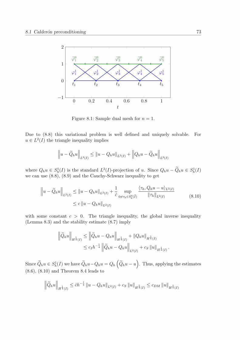
8.1 Calderon preconditioning 73
0 0.2 0.4 0.6 0.8 1−1
0
1
2
t1 t2 t3 t4 t5
ϕ11 ϕ1
2 ϕ13 ϕ1
4 ϕ15
ϕ01 ϕ0
2 ϕ03 ϕ0
4 ϕ05
t
Figure 8.1: Sample dual mesh for n = 1.
Due to (8.8) this variational problem is well defined and uniquely solvable. Foru ∈ L2(I) the triangle inequality implies∥∥∥u− Qhu
∥∥∥L2(I)
≤ ‖u−Qhu‖L2(I) +∥∥∥Qhu− Qhu
∥∥∥L2(I)
where Qhu ∈ S1h(I) is the standard L2(I)-projection of u. Since Qhu − Qhu ∈ S1
h(I)we can use (8.8), (8.9) and the Cauchy-Schwarz inequality to get
∥∥∥u− Qhu∥∥∥L2(I)
≤ ‖u−Qhu‖L2(I) +1
csup
06=τh∈S0h(I)
〈τh, Qhu− u〉L2(I)
‖τh‖L2(I)
≤ c ‖u−Qhu‖L2(I)
(8.10)
with some constant c > 0. The triangle inequality, the global inverse inequality(Lemma 8.3) and the stability estimate (8.7) imply∥∥∥Qhu
∥∥∥H
14 (I)≤∥∥∥Qhu−Qhu
∥∥∥H
14 (I)
+ ‖Qhu‖H 14 (I)
≤ cIh− 1
4
∥∥∥Qhu−Qhu∥∥∥L2(I)
+ cS ‖u‖H 14 (I)
.
Since Qhu ∈ S1h(I) we have Qhu−Qhu = Qh
(Qhu− u
). Thus, applying the estimates
(8.6), (8.10) and Theorem 8.4 leads to∥∥∥Qhu∥∥∥H
14 (I)≤ ch−
14 ‖u−Qhu‖L2(I) + cS ‖u‖H 1
4 (I)≤ cDM ‖u‖H 1
4 (I)

74 8 Preconditioning
with some constant cDM > 0. Hence for τh ∈ S0h(I) we have
‖τh‖H− 14 (I)
= sup0 6=v∈H
14 (I)
〈τh, v〉L2(I)
‖v‖H
14 (I)
= sup0 6=v∈H
14 (I)
〈τh, Qhv〉L2(I)
‖v‖H
14 (I)
≤ cDM sup06=v∈H
14 (I)
〈τh, Qhv〉L2(I)∥∥∥Qhv∥∥∥H
14 (I)
≤ cDM sup06=vh∈S1
h(I)
〈τh, vh〉L2(I)
‖vh‖H 14 (I)
which concludes the proof.
Consequently, when discretizing V in the space S0h(I) and D in the space S1
h(I)the preconditioner C−1
V = M−1h DhM
−Th leads to a bounded condition number of the
preconditioned system matrix. As in the case of piecewise linear basis functions this ap-proach is a suitable preconditioning technique for n = 2, 3 as well. Since the boundaryelements of the dual mesh are of arbitrary form (polygonial), we need approximationproperties of trial spaces corresponding to the dual mesh in anisotropic Sobolev spaces.

9 FEM-BEM coupling
In this chapter we present and discuss a FEM-BEM coupling method for parabolictransmission problems, based on [3]. As in the case of stationary transmission problems[24] we can derive boundary integral equations for the exterior problem and use acoupling method to solve the integral equations in combination with a finite elementdiscretization of the interior problem [29]. We consider a non-symmetric FEM-BEMcoupling method. In addition to the derivation of a variational formulation for thecoupled problem we consider a Galerkin method in order to discretize the problemand compute an approximation of the solution.
9.1 Model problem
Let f ∈ L2(0, T ;H−1(Ω)) and u0 ∈ H10 (Ω). We consider the transmission problem
α∂tui(x, t)− divx [A(x, t)∇xui(x, t)] = f(x, t) for (x, t) ∈ Ω× (0, T ),
α∂tue(x, t)−∆ue(x, t) = 0 for (x, t) ∈ Ωext × (0, T ),
ui(x, 0) = u0(x) for x ∈ Ω,
ue(x, 0) = 0 for x ∈ Ωext
(9.1)
with Ωext := Rn \ Ω and transmission conditions
ui(x, t) = ue(x, t), nx · [A(x, t)∇xui(x, t)] =∂
∂nxue(x, t) =: we(x, t) (9.2)
for (x, t) ∈ Σ. We assume, that the coefficient matrix A(x, t) ∈ Rn×n is symmetricand uniform positive definite, i.e. there exists θ > 0 such that
θ|ξ|2 ≤ [A(x, t) ξ] · ξ
for all (x, t) ∈ Q and all ξ ∈ Rn. The solution ue of the exterior problem satisfiesa radiation condition for |x| → ∞ and t ∈ (0, T ). Similarly to the initial boundaryvalue problem (2.1) we can derive a representation formula for the solution ue of the
75

76 9 FEM-BEM coupling
exterior problem [3]. For (x, t) ∈ Ωext × (0, T ) we have
ue(x, t) =− 1
α
T∫0
∫Γ
U∗(x− y, t− s) ∂
∂nyue(y, s)dsyds
+1
α
T∫0
∫Γ
∂
∂nyU∗(x− y, t− s)ue(y, s)dsyds.
(9.3)
By applying the Dirichlet trace operator and using the jump relations (5.4) and (5.7)we get the first boundary integral equation for the exterior problem
γext0 ue = −V γext
1 ue +
(1
2I +K
)γext
0 ue on Σ. (9.4)
9.2 Coupling
First we consider the initial boundary value problem
α∂tui(x, t)− divx [A(x, t)∇xui(x, t)] = f(x, t) for (x, t) ∈ Ω× (0, T )
ui(x, 0) = u0(x) for x ∈ Ω(9.5)
with f ∈ L2(0, T ;H−1(Ω)), u0 ∈ H10 (Ω) and the Neumann boundary condition
nx · [A(x, t)∇xui(x, t)] = wi(x, t) for (x, t) ∈ Γ× (0, T ).
The variational formulation is to find ui ∈ L2(0, T ;H1(Ω)) ∩ H1(0, T ; H−1(Ω)) withui(x, 0) = u0(x) for x ∈ Ω such that
a(ui, v) =
∫ T
0
∫Ω
f(x, t), v(x, t)dxdt+
∫ T
0
∫Γ
wi(x, t)v(x, t)dsxdt
for all v ∈ L2(0, T ;H1(Ω)). The bilinear form a(·, ·) is given by
a(u, v) :=
∫ T
0
∫Ω
α∂tui(x, t)v(x, t)dxdt+
∫ T
0
∫Ω
[A(x, t)∇xui(x, t)] · ∇xv(x, t)dxdt
for u ∈ L2(0, T ;H1(Ω)) ∩ H1(0, T ; H−1(Ω)) und v ∈ L2(0, T ;H1(Ω)). Due to theinitial condition in (9.5) we consider the decomposition ui(x, t) = ui(x, t) + u0(x, t)
for (x, t) ∈ Q where u0 ∈ L2(0, T ;H10 (Ω)) ∩ H1(0, T ; H−1(Ω)) is an extension of the
initial condition u0 ∈ H10 (Ω) into the space-time cylinder Q. Hence we want to find
ui ∈ L2(0, T ;H1(Ω)) ∩H1(0, T ; H−1(Ω)) with ui(x, 0) = 0 for x ∈ Ω such that
a(ui, v)− 〈wi, γint0 v〉Σ = 〈f, v〉Q − a(u0, v) for all v ∈ L2(0, T ;H1(Ω)).

9.3 Discretization 77
For details regarding existence and uniqueness of solutions, see [29] and [30]. Let X
be the Dirichlet trace space of L2(0, T ;H1(Ω)) ∩ H1(0, T ; H−1(Ω)). The variationalformulation of the boundary integral equation (9.4) is to find we ∈ X ′ such that
〈V we, τ〉Σ + 〈(
1
2I −K
)γext
0 ue, τ〉Σ = 0 for all τ ∈ X ′.
Together with the transmission conditions (9.2) we get the variational formulation of
the coupled problem. We have to find ui ∈ L2(0, T ;H1(Ω)) ∩H1(0, T ; H−1(Ω)) withui(x, 0) = 0 for x ∈ Ω and we ∈ X ′ such that
a(ui, v)− 〈we, γint0 v〉Σ = 〈f, v〉Q − a(u0, v),
〈V we, τ〉Σ + 〈(
1
2I −K
)γint
0 ui, τ〉Σ = 0(9.6)
for all v ∈ L2(0, T ;H1(Ω)) and τ ∈ X ′.
9.3 Discretization
We consider an admissible triangulation Th = qlNQl=1 of the space-time cylinder Q into
finite elements ql. Let (xk, tk)MQ
k=1 be the set of nodes of the triangulation. We defineI0 to be the index set of the nodes, which do not belong to Ω × 0 and M0 := |I0|.Moreover II is the index set of the nodes, which do not belong to Σ ∪
(Ω× 0
)and MI := |II |. The nodes are sorted in such a way, that I0 ⊂ 1, ...,M0 andII ⊂ 1, ...,MI. The boundary elements Eh = σkNΣ
k=1 of the induced decompositionof Σ are given by
Eh :=σ ⊂ Σ : ∃ q ∈ Th : σ = ∂q ∩ Σ
.
Figure 9.1 shows a sample triangulation for the spatially one-dimensional problem.Let S0
h(Σ) = span ϕ0k
NΣ
k=1 be the space of piecewise constant basis function withrespect to the triangulation Eh of the boundary Σ, i.e. we have
ϕ0k(x, t) :=
1 for (x, t) ∈ σk,0 else
for k = 1, ..., NΣ and S1h(Q) = span ϕ1
i MQ
i=1 be the space of piecewise linear andcontinuous basis functions ϕ1
i with respect to the triangulation Th of the space-timecylinder Q, i.e.
ϕ1i (xj, tj) = δij for i, j = 1, ...,MQ,
where (xj, tj) ∈ Rn+1 are the coordinates of the j-th node of Th, see [34]. Moreover wedefine S1
h,0(Q) to be the space of functions in S1h(Q), which vanish on Ω × 0. Due

78 9 FEM-BEM coupling
0 0.2 0.4 0.6 0.8 1
0
0.2
0.4
0.6
0.8
1
x
tThEh
Nodes I0
Nodes II
Figure 9.1: Sample triangulation of Q = (0, 1)× (0, 1).
to the sorting of the nodes we have S1h,0(Q) = span ϕ1
i M0
i=1. We approximate we andui by
we,h =
NΣ∑k=1
wkϕ0k ∈ S0
h(Σ), ui,h =
M0∑j=1
ujϕ1j ∈ S1
h,0(Q).
Hence it remains to compute the unknown coefficients wk and uj.
9.4 Galerkin method
Let u0,h be the interpolation of u0 in S1h(Q), i.e. we have
u0,h =
MQ∑j=1
uj0ϕ1j
with uj0 = u0(xj, tj) for j = 1, ...,MQ. Since u0 ∈ L2(0, T ;H10 (Ω)) ∩H1(0, T ; H−1(Ω))
we have uj0 = 0 for xj ∈ Γ. The Galerkin variational formulation of (9.6) is to findui,h ∈ S1
h,0(Q) and we,h ∈ S0h(Σ) such that
a(ui,h, vh)− 〈we,h, vh〉Σ = 〈f, vh〉Q − a(u0,h, vh),
〈V we,h, τh〉Σ + 〈(
1
2I −K
)ui,h, τh〉Σ = 0

9.4 Galerkin method 79
for all v ∈ S1h,0(Q) and for all τh ∈ S0
h(Σ). This formulation is equivalent to the systemof linear equationsAQQ AQΣ
AΣQ AΣΣ −MTh
12Mh −Kh Vh
uQ
uΣ
w
=
fQ
fΣ
0
(9.7)
with
A[j, i] = a(ϕ1i , ϕ
1j), u[j] = uj + uj0, f [j] = 〈f, ϕ1
j〉Q −MQ∑
r=M0+1
ur0 a(ϕ1r, ϕ
1j)
for i, j = 1, ...,M0, where uj0 = 0 for xj ∈ Γ, and
Mh[l, i] = 〈ϕ1MI+i, ϕ
0l 〉Σ, Kh[l, i] = 〈Kϕ1
MI+i, ϕ0l 〉Σ, Vh[l, k] = 〈V ϕ0
k, ϕ0l 〉Σ
for i = 1, ...,M0 −MI and k, l = 1, ..., NΣ.
Consequently we can compute the unkown coefficients wk and uj and the correspond-ing approximations we,h and ui,h. The solution ui,h of the interior transmission problem(9.1) is then given by ui,h = ui,h+u0,h, whereas the solution ue,h of the exterior problemis given by the representation formula (9.3), i.e. we have
ue,h(x, t) = −(V we,h)(x, t) + (Wγint0 ui,h)(x, t) for (x, t) ∈ Ωext × (0, T ).


10 Numerical examples
In this chapter we present numerical examples regarding the convergence proper-ties of the Galerkin approximations and the preconditioning techniques for the one-dimensional heat equation as well as examples for the FEM-BEM coupling method.
10.1 Preconditioning
Let Ω = (0, 1) and T = 1. In general we consider the initial boundary value problem
α∂tu(x, t)− ∂xxu(x, t) = 0 for (x, t) ∈ (0, 1)× (0, 1),
u(0, t) = u(1, t) = 0 for t ∈ (0, 1),
u(x, 0) = u0(x) for x ∈ (0, 1)
(10.1)
where u0 is some given initial condition satisfying u0(0) = u0(1) = 0. The solution uis given by the representation formula
u(x, t) = (V γint1 u)(x, t) + (M0u0)(x, t) for (x, t) ∈ (0, 1)× (0, 1).
We use the variational formulation of the first boundary integral equation (7.1) to de-
termine the unknown conormal derivative γint1 u, i.e. we have to find γint
1 u ∈ H− 12,− 1
4 (Σ)such that
〈V γint1 u, τ〉Σ = −〈M0u0, τ〉Σ for all τ ∈ H−
12,− 1
4 (Σ).
For the discretization of this formulation we consider the space of piecewise constantbasis functions S0
h(Σ). This leads to the system of linear equations
Vhw = f (10.2)
where
Vh[l, k] = 〈V ϕ0k, ϕ
0l 〉Σ =
∫Σ
(V ϕ0k)(x, t)ϕ
0l (x, t)dsxdt
=1
αnlnk
∫ tl2
tl1
∫ tk2
tk1
U?(xl − xk, t− s)dsdt
and
f [l] = −〈M0u0, ϕ0l 〉Σ = −
∫Σ
(M0u0)(x, t)ϕ0l (x, t)dsxdt
= −nl∫ tl2
tl1
∫ 1
0
U?(xl − y, t)u0(y)dydt
81

82 10 Numerical examples
for l, k = 1, ..., N . The Galerkin approximation wh of the conormal derivative w = γint1 u
is then given by
wh(x, t) =N∑l=1
wlϕ0l (x, t) for (x, t) ∈ Σ.
The system (10.2) is solved with the GMRES method. We want the condition numberto be independent of the mesh size h. Therefore we use the preconditioning techniqueintroduced in Chapter 8. In the one-dimensional case we can use the piecewise constantbasis functions to discretize the hypersingular operator D. The preconditioner is givenby
C−1V = M−1
h DhM−Th
where
Dh[l, k] = 〈Dϕ0k, ϕ
1l 〉Σ =
∫Σ
(Dϕ0k)(x, t)ϕ
0l (x, t)dsxdt = nl
∫ tl2
tl1
(Dϕ0k)(xl, t)dt
and
Mh[l, k] = 〈ϕ0k, ϕ
0l 〉L2(Σ) =
∫Σ
ϕ0k(x, t)ϕ
0l (x, t)dsxdt
=
|tl2 − tl1 | if l = k,
0 if l 6= k.
Since Mh is a diagonal matrix, the computation of the inverse of Mh and the compu-tation of the preconditioning matrix C−1
V respectively is quite fast and very simple.
Uniform refinement
First we consider the initial boundary value problem (10.1) with initial conditionu0(x) = sin (2πx) ∈ H1
0 (Ω) und use a uniform refinement strategy to compute theapproximation wh. The unique solution of this problem is shown in Figure 10.1. Table10.1 shows the L2(Σ)-error and the corrensponding convergence, the condition numbersof the system matrix and the preconditioned matrix, as well as the iteration numbers ofthe GMRES method in both cases. We obtain linear convergence of the approximation,which is what we expected according to Theorem (7.9). While we can see that thecondition number of the matrix Vh is increasing with a factor of approximately
√2, the
condition number of the preconditioned matrix C−1V Vh is bounded. Hence the iteration
number of the preconditioned system is bounded as well, while the iteration numbercorresponding to (10.2) is increasing with a factor of approximately 4
√2.

10.1 Preconditioning 83
Figure 10.1: Uniform refinement. Approximation uh at level 11.
L N ‖w − wh‖L2(Σ) eoc κ(Vh) Factor It. Factor κ(C−1V Vh) It.
0 2 2,249 0 1,001 0 1 0 1,002 1
1 4 1,311 0,778 2,808 2,807 2 2 1,279 2
2 8 0,658 0,996 4,905 1,746 4 2 1,422 4
3 16 0,324 1,021 7,548 1,539 8 2 1,486 8
4 32 0,16 1,017 11,14 1,476 16 2 1,541 14
5 64 0,079 1,01 16,724 1,501 31 1,938 1,563 13
6 128 0,04 1,006 13,47 0,805 41 1,323 1,59 13
7 256 0,02 1,003 22,053 1,637 50 1,22 1,615 12
8 512 0,01 1,001 32,043 1,453 59 1,18 1,636 12
9 1024 0,005 1,001 60,957 1,902 70 1,186 1,777 11
10 2048 0,002 1,000 88,488 1,452 82 1,171 1,762 11
11 4096 0,001 1,000 125,957 1,423 96 1,171 1,765 10
Table 10.1: Uniform refinement. Condition and iteration numbers.

84 10 Numerical examples
The unique solution of the initial boundary value problem (10.1) with initial conditionu0 = 0 is u = 0. Thus, we have γint
1 u = 0. Table 10.2 shows the iteration numbers ofthe GMRES method using a random initial guess. Again, we obtain boundedness ofthe iteration numbers corresponding to the preconditioned system. We can concludethat the results concerning the iteration numbers in the previous example do notdepend on the given data.
L N It. Factor It. Prec.
0 2 2 0 21 4 3 1,5 32 8 4 1,333 43 16 8 2 84 32 16 2 135 64 31 1,938 146 128 42 1,355 137 256 52 1,238 138 512 64 1,231 139 1024 77 1,203 1310 2048 92 1,195 1311 4096 109 1,185 12
Table 10.2: Iteration numbers for a random initial guess of the GMRES.
Adaptive refinement
We consider problem (10.1) with initial condition u0 = 5 exp (−10x) sin (πx) and usean adaptive refinement strategy to compute the approximation wh.Let N ∈ N and ΣN be a decomposition of Σ into N boundary elements σl as given by(7.14), i.e. we have
ΣN =N⋃l=1
σl.
Let w = γint1 u ∈ H− 1
2,− 1
4 (Σ) be the exact solution and wh =∑N
l=1wlϕ0l ∈ S0
h(Σ) be theGalerkin approximation of the problem. The local L2(Σ)-error on a boundary elementσl is then given by
el := ‖w − wh‖L2(σl).
The strategy is to refine each boundary element σl whose error satisfies
el ≥ θ maxk=1,...,N
ek

10.1 Preconditioning 85
with parameter θ ∈ (0, 1). In our case we divide those elements into two elements ofsame size. We continue to refine the mesh until the global error
e :=
(N∑l=1
e2l
) 12
is less than some given value. Of course, in general we do not know the exact solutionof the problem. Thus, we have to use a posteriori error estimators, see for example [6]and [23].According to Section 2.1.1 the exact solution of the problem (10.1) is given by theseries
u(x, t) =∞∑k=1
ak exp
(−(kπ)2t
α
)sin (kπx) for (x, t) ∈ Q
with
ak = 2
∫ 1
0
u0(x) sin (kπx)dx.
Hence the conormal derivative w = ∂nu|Σ is given by
∂nu(x, t) = nx
∞∑k=1
ak exp
(−(kπ)2t
α
)kπ cos (kπx) for (x, t) ∈ Σ
where nx = −1 for x = 0 and nx = 1 for x = 1. The solution uh of the problem(10.1) is shown in Figure 10.2. Figure 10.3 shows the approximation wh of the conor-mal derivative. In Table 10.3 you can see the L2(Σ)-error, the condition numbers ofthe system matrix and the preconditioned matrices, as well as the iteration numbersof the GMRES method. In addition to the Calderon preconditioner the conditionand iteration numbers of the diagonally scaled system matrix is listed in the table.As in the case of uniform refinement we obtain boundedness of the condition num-ber of the Calderon-preconditioned matrix C−1
V Vh, as well as the boundedness of thecorresponding iteration numbers of the GMRES method. Diagonal scaling causes animprovement concerning the condition numbers of the system matrix and the iterationnumbers of the GMRES method.

86 10 Numerical examples
Figure 10.2: Adaptive refinement. Approximation uh at level 10.
0 0.2 0.4 0.6 0.8 1
0
2
4
6
8
10
12
14
t
t h(·,t)
x = 0x = 1
Figure 10.3: Adaptive refinement. Approximation wh at level 10.

10.2 FEM-BEM coupling 87
CV = diagVh CV = MhD−1h Mh
L N ‖w − wh‖L2(Σ) κ(Vh) It. κ(C−1V Vh) It. κ(C−1
V Vh) It.
0 2 1,886 1,001 2 1,001 2 1,002 2
1 3 1,637 3,972 3 2,553 3 1,16 3
2 5 1,272 12,225 5 4,055 4 1,166 4
3 7 0,914 34,212 7 3,611 6 1,156 6
4 9 0,615 92,081 9 3,164 8 1,149 8
5 11 0,401 118,586 11 2,945 10 1,224 10
6 13 0,267 338,26 13 2,803 12 1,21 12
7 20 0,166 621,773 20 3,524 18 1,197 13
8 31 0,101 1608,08 31 4,457 27 1,252 12
9 47 0,063 2344,9 47 5,779 32 1,574 11
10 74 0,039 6141,47 74 8,348 37 1,692 11
11 114 0,024 8409,92 114 10,95 42 1,561 10
12 177 0,015 23007,6 173 14,324 47 1,716 10
13 278 0,01 27528,3 200 21,094 53 1,677 10
Table 10.3: Adaptive refinement. Condition and iteration numbers.
10.2 FEM-BEM coupling
For Ω = (0, 1) and T = 1 we consider the one-dimensional transmission problem
α∂tui(x, t)− ∂x [A(x)∂xui(x, t)] = f(x, t) for (x, t) ∈ Ω× (0, 1),
α∂tue(x, t)− ∂xxue(x, t) = 0 for (x, t) ∈ Ωext × (0, 1),
ui(x, 0) = u0(x) for x ∈ Ω,
ue(x, 0) = 0 for x ∈ Ωext
(10.3)
where f ∈ L2(0, T ;H−1(Ω)) and u0 ∈ H1(Ω) are given. The following examples referto the initial triangulation shown in Figure 9.1 and a uniform refinement strategy.The tables show the L2(Q)-error ‖ui − ui,h‖L2(Q) and the corresponding convergence
of the approximation of the interior problem. The L2(Q)-error was computed with the7-point rule [33, Section C.1]. The system of linear equations (9.7) was solved withPARDISO Version 5.0.0 [11, 21, 22].

88 10 Numerical examples
Initial condition u0 continuously differentiable
We consider the transmission problem (10.3) with A ≡ 1, f ≡ 0 and initial condition
u0(x) =
exp
(1
(2x− 1)2 − 1
)sin (πx) for x ∈ (0, 1),
0 else.
Figure 10.4 shows the approximation uh of the solution of the transmission problem(10.3). The L2(Q)-errors and the estimated orders of convergence are listed in Table10.4. As expected we get an order of convergence of 2 for the Galerkin approximationof the interior problem.
Level MQ NQ NΣ ‖ui − ui,h‖L2(Q) eoc
0 9 8 4 0.0316182 01 25 32 8 0.015779 1.002752 81 128 16 0.00422301 1.901663 289 512 32 0.00111947 1.915454 1089 2048 64 0.000289581 1.950785 4225 8192 128 7.3735e-05 1.97355
Table 10.4: Error and convergence of ui,h.
Figure 10.4: Approximation uh at level 5.
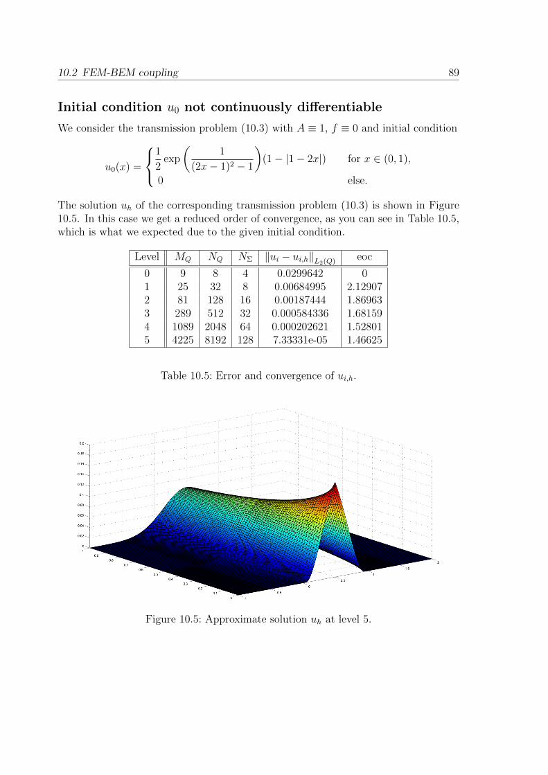
10.2 FEM-BEM coupling 89
Initial condition u0 not continuously differentiable
We consider the transmission problem (10.3) with A ≡ 1, f ≡ 0 and initial condition
u0(x) =
1
2exp
(1
(2x− 1)2 − 1
)(1− |1− 2x|) for x ∈ (0, 1),
0 else.
The solution uh of the corresponding transmission problem (10.3) is shown in Figure10.5. In this case we get a reduced order of convergence, as you can see in Table 10.5,which is what we expected due to the given initial condition.
Level MQ NQ NΣ ‖ui − ui,h‖L2(Q) eoc
0 9 8 4 0.0299642 01 25 32 8 0.00684995 2.129072 81 128 16 0.00187444 1.869633 289 512 32 0.000584336 1.681594 1089 2048 64 0.000202621 1.528015 4225 8192 128 7.33331e-05 1.46625
Table 10.5: Error and convergence of ui,h.
Figure 10.5: Approximate solution uh at level 5.


11 Conclusion and Outlook
In this work we presented the boundary element method for the discretization of thetime-dependent heat equation. After the derivation of the representation formula forthe solution of the model problem (2.1) we analysed the heat potentials and the bound-ary integral operators in the setting of anisotropic Sobolev spaces. We have shown,that the single layer boundary integral operator V and the hypersingular operatorD are elliptic and bounded and therefore invertible. We presented four different ap-proaches for the computation of the unkown conormal derivative ∂nu|Σ. We discusseddirect approaches using the boundary integral equations (6.3) as well as indirect for-mulations with the single layer potential and the double layer potential. All fourformulations are uniquely solvable.We considered a Galerkin-Bubnov variational formulation of the first boundary inte-gral equation (7.17) and concluded unique solvability of the discrete problem due tothe ellipticity and boundedness of the operator V . As a trial space we used the space ofpiecewise constant basis functions S0
h(Σ) corresponding to an arbitrary triangulationof the space-time boundary Σ for the one- and two-dimensional problem, see Section7.1. In the two-dimensional case we made an assumption on the form and orientationof the boundary elements, see Figure 7.1, and derived the approximation propertiesof S0
h(Σ) by using the approximation properties of space-time tensor product spaces.The extension of those approximation properties to trial spaces with respect to trian-gulations with boundary elements of arbitrary form and orientation for n = 2 as wellas for n = 3 is still open.We estimated the error of the Galerkin approximations in the energy norm and statedan estimate for the L2(Σ)-error of the approximations for the one-dimensional problemby using the inverse inequality (7.9). If we can prove an inverse inequality for functionsin S0
h(Σ) for n = 2, 3 in the setting of anisotropic Sobolev spaces, we are able to givean L2(Σ)-error estimate for n = 2, 3 as well.We used the GMRES method to solve the system of linear equations (7.18). Since thecondition number of the matrix Vh depends on the mesh size h of the decomposition ofΣ we applied the Calderon preconditioning strategy and used the discretization of thehypersingular operator D as a preconditioner for Vh, see Chapter 8. We discussed theone-dimensional problem and presented three different approaches for the discretiza-tion of V and D. If we can prove stability of the L2(Σ)-projection onto the spaceof piecewise linear and continuous basis functions in the anisotropic Sobolev spaceH
12, 14 (Σ) some of the results can be extended to n = 2, 3. However, this is still an open
issue.
91

92 11 Conclusion and Outlook
In Chapter 9 we presented the concept of a non-symmetric FEM-BEM couplingmethod for the parabolic transmission problem (9.1) and described a Galerkin methodfor the discretization of the coupled problem. It is still an open question how to char-acterize the trace spaces of the Bochner spaces used for the variational formulation ofthe interior problem and if the operator V is elliptic in this setting as well.In Chapter 10 we introduced an adaptive refinement strategy but used the exact solu-tion to get an error estimator. Of course in general we do not know the exact solution.Thus, we have to establish a posteriori error estimators for the anisotropic BEM inorder to define adaptive refinement strategies.
Bibliography
[1] W. Arendt and K. Urban. Partielle Differenzialgleichungen. Springer Spektrum,Heidelberg, 2010.
[2] M. Costabel. Boundary integral operators for the heat equation. Integral Equa-tions and Operator Theory, 13:498–552, 1990.
[3] S. Dohr. Raum-Zeit FEM-BEM-Kopplung fur parabolische Transmissionsprob-leme. Projekt TM, Institut fur Numerische Mathematik, Technische UniversitatGraz, 2016.
[4] J. Elstrodt. Maß- und Integrationstheorie. Springer, Berlin-Heidelberg, 2010.
[5] L. C. Evans. Partial Differential Equations. Graduate Studies in Mathematics,19, 1997.
[6] S. Ferraz-Leite and D. Praetorius. Simple a posteriori error estimators for theh-version of the boundary element method. Computing, 83:135–162, 2008.
[7] A. Friedman. Partial Differential Equations of Parabolic Type. R. E. KriegerPublishing Company, Malabar, Florida, 1983.
[8] M. Hamina. Some boundary element methods for heat conduction problems.Thesis, University of Oulu, 2000.
[9] R. Hiptmair. Operator Preconditioning. Computers and Mathematics with Ap-plications, 52:699–706, 2006.
[10] R. Hiptmair, C. Jerez-Hanckes and C. Urzua. Mesh-Independent Operator Pre-conditioning for Boundary Elements on Open Curves. SIAM Journal on Numer-ical Analysis, 52:2295–2314, 2014.
[11] G. Karypis and V. Kumar. A fast and high quality multilevel scheme for parti-tioning irregular graphs. SIAM Journal on Scientific Computing, 20(1):359–392,1999.
[12] J. L. Lions and E. Magenes. Non-Homogeneous Boundary Value Problems andApplications. Volume I. Springer, Berlin-Heidelberg-New York, 1972.
[13] J. L. Lions and E. Magenes. Non-Homogeneous Boundary Value Problems andApplications. Volume II. Springer, Berlin-Heidelberg-New York, 1972.
[14] W. McLean. Strongly Elliptic Systems and Boundary Integral Equations. Cam-bridge University Press, 2000.
93

94 Bibliography
[15] M. Meßner. A Fast Multipole Galerkin Boundary Element Method for the Tran-sient Heat Equation. Monographic Series TU Graz: Computation in Engineeringand Science, 23, 2014.
[16] M. Neumuller. Space-Time Methods. Monographic Series TU Graz: Computationin Engineering and Science, 20, 2013.
[17] P.J. Noon. The Single Layer Heat Potential and Galerkin Boundary ElementMethods for the Heat Equation. Thesis, University of Maryland, 1988.
[18] T. X. Phan. Boundary Element Methods for Boundary Control Problems. Mono-graphic Series TU Graz: Computation in Engineering and Science, 9, 2011.
[19] W. Pogorzelski. Integral Equations and their Applications. Pergamon Press,Oxford, 1966.
[20] A. Reinarz. Sparse Space-time Boundary Element Methods for the Heat Equation.Thesis, University of Reading, 2015.
[21] O. Schenk and K. Gartner. Solving unsymmetric sparse systems of linearequations with PARDISO. Journal of Future Generation Computer Systems,20(3):475–487, 2004.
[22] O. Schenk and K. Gartner. On fast factorization pivoting methods for symmetricindefinite systems. Elec. Trans. Numer. Anal., 23:158–179, 2006.
[23] H. Schulz and O. Steinbach. A new a posteriori error estimator in adaptive directboundary element methods: the Dirichlet problem. CALCOLO, 37:79–96, 2000.
[24] G. Of, G. Rodin, O. Steinbach and M. Taus. Coupling of Discontinuous GalerkinFinite Element and Boundary Element Methods. SIAM Journal on ScientificComputing, 34(3):A1659–A1677, 2012.
[25] O. Steinbach. On the stability of the L2 projection in fractional Sobolev spaces.Numerische Mathematik, 88:367–379, 2001.
[26] O. Steinbach. On a generalized L2 projection and some related stability estimatesin Sobolev spaces. Numerische Mathematik, 90:775–786, 2002.
[27] O. Steinbach. Numerische Naherungsverfahren fur elliptische Randwertprobleme.Finite Elemente und Randelemente. B.G. Teubner, Stuttgart-Leipzig-Wiesbaden,2003.
[28] O. Steinbach. Stability Estimates for Hybrid Coupled Domain DecompositionMethods. Springer, Berlin-Heidelberg-New York, 2003.
[29] O. Steinbach. Space-Time Finite Element Methods for Parabolic Problems. Com-putational Methods in Applied Mathematics, 15:551–566, 2015.
[30] O. Steinbach. Space time discretizations for Partial Differential Equations, Lec-ture Notes. Technische Universitat Graz, 2016.
Bibliography 95
[31] O. Steinbach and W. L. Wendland. The construction of some efficient precondi-tioners in the boundary element method. Advances in Computational Mathemat-ics, 9:191–216, 1998.
[32] V. Thomee. Galerkin Finite Element Methods for Parabolic Problems. Springer,Berlin-Heidelberg, 2006.
[33] S. Rjasanow und O. Steinbach. The Fast Solution of Boundary Integral Equations.Springer, New York, 2007.
[34] G. Unger. Numerische Mathematik 3, Vorlesungsskript. Technische UniversitatGraz, 2014.
[35] D. Werner. Funktionalanalysis. Springer, Berlin-Heidelberg, 2011.


Eidesstattliche Erklarung
Ich erklare an Eides statt, dass ich die vorliegende Arbeit selbstandig verfasst, andereals die angegebenen Quellen/Hilfsmittel nicht benutzt, und die den benutzten Quellenwortlich und inhaltlich entnommenen Stellen als solche kenntlich gemacht habe. Dasin TUGRAZonline hochgeladene Textdokument ist mit der vorliegenden Masterarbeitidentisch.
Datum Unterschrift


![A Boundary Element Model for Underwater Acoustics in ... · equation [Kinsler, Frey, Coppens and Sanders (1982)]:](https://img.pdfslide.us/doc/110x75/5b84191f7f8b9ad34a8b85a9/a-boundary-element-model-for-underwater-acoustics-in-equation-kinsler.jpg)