Finite element method 1 Finite Elements Basic formulation Basis functions Stiffness matrix Poisson‘s equation Regular grid Boundary conditions

1Finite element method

Finite Elements

Basic formulation Basis functions Stiffness matrix Poisson‘s equation

Regular grid Boundary conditions Irregular grid

Numerical Examples

Scope: Understand the basic concept of the finite element method with the simple-most equation.


Formulation

Let us start with a simple linear system of equations

| * y

and observe that we can generally multiply both sides of this equation with y without changing its solution. Note that x,y and b are vectors and A is a matrix.

bAx

nyybyAx

We first look at Poisson’s equation

)()( xfxu where u is a scalar field, f is a source term and in 1-D

2

22

x


Poisson‘s equation

fvuv

We now multiply this equation with an arbitrary function v(x), (dropping the explicit space dependence)

... and integrate this equation over the whole domain. For reasons of simplicity we define our physical domain D in the interval [0, 1].

DD

fvuv

dxfvdxuv 1

0

1

0

Das Reh springt hoch,

das Reh springt weit,

warum auch nicht,

es hat ja Zeit.

... why are we doing this? ... be patient ...


Discretization

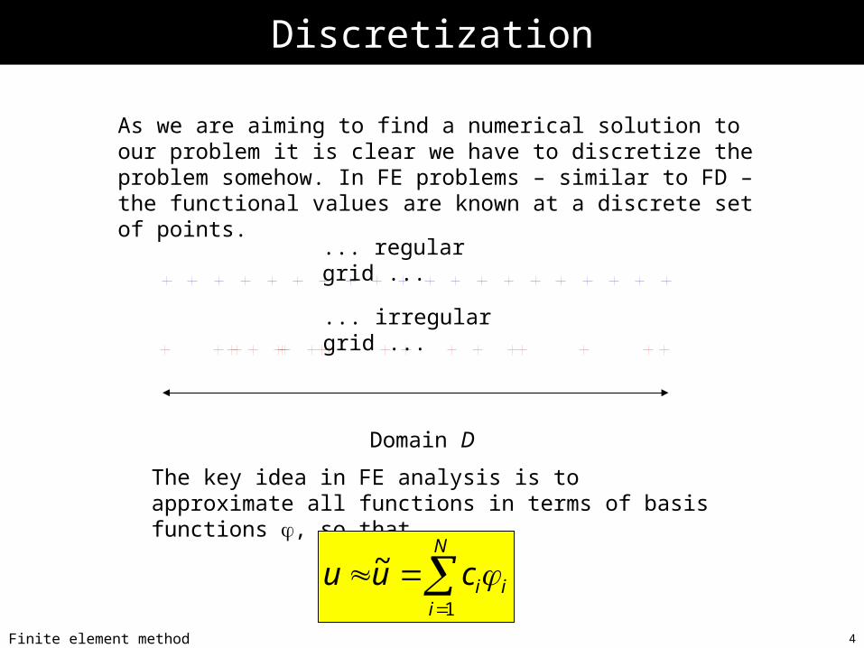
As we are aiming to find a numerical solution to our problem it is clear we have to discretize the problem somehow. In FE problems – similar to FD – the functional values are known at a discrete set of points.

... regular grid ...

... irregular grid ...

Domain D

The key idea in FE analysis is to approximate all functions in terms of basis functions , so that

i

N

iicuu

1

~


Basis function

where N is the number nodes in our physical domain and ci are real constants.

With an appropriate choice of basis functions i, the coefficients ci are equivalent to the actual function values at node point i. This – of course – means, that i=1 at node i and 0 at all other nodes ...

Doesn’t that ring a bell?

Before we look at the basis functions, let us ...

i

N

iicuu

1

~


Partial Integration

... partially integrate the left-hand-side of our equation ...

dxfvdxuv 1

0

1

0

dxuvuvdxvu 1

0

10

1

0

)(

we assume for now that the derivatives of u at the boundaries vanish so that for our particular problem

dxuvdxvu 1

0

1

0

)(


…

... so that we arrive at ...

... with u being the unknown. This is also true for our approximate numerical system

dxfvdxvu 1

0

1

0

... where ...

i

N

iicu

1

~

was our choice of approximating u using basis functions.

dxfvdxvu 1

0

1

0

~


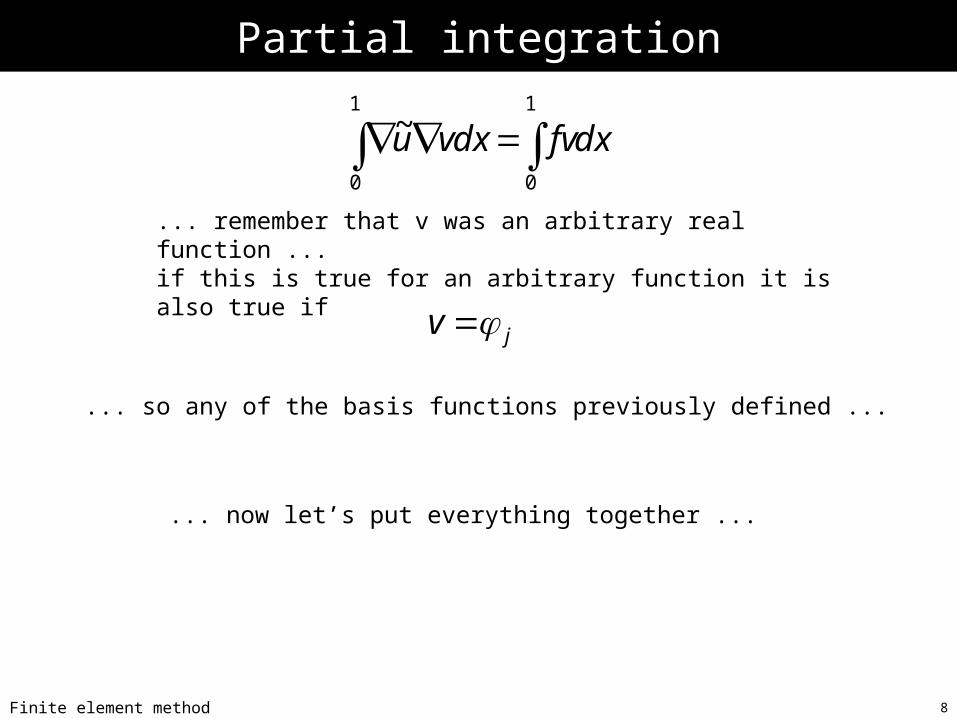
Partial integration

... remember that v was an arbitrary real function ... if this is true for an arbitrary function it is also true if

... so any of the basis functions previously defined ...

jv

... now let’s put everything together ...

dxfvdxvu 1

0

1

0

~


The discrete system

The ingredients:

kv i

N

iicu

1

~

dxfvdxvu 1

0

1

0

~

dxfdxc kk

n

iii

1

0

1

0 1

... leading to ...


The discrete system

dxfdxc kki

n

ii

1

0

1

01

... the coefficients ck are constants so that for one particular function k this system looks like ...

kiki gAb ... probably not to your surprise this can be written in matrix form

kiTik gbA


The solution

... with the even less surprising solution

kTiki gAb

1

remember that while the bi’s are really the coefficients of the basis functions these are the actual function values at node points i as well

because of our particular choice of basis functions.

This become clear further on ...


Basis functions

... otherwise we are free to choose any function ...

The simplest choice are of course linear functions:

+ grid nodes

blue lines – basis functions i

1

2

3

4

5

6

7

8

9

10

we are looking for functions i

with the following property

ijxxfor

xxforx

j

ii ,0

1)(


Basis functions - gradient

To assemble the stiffness matrix we need the gradient (red) of the basis functions (blue)

1

2

3

4

5

6

7

8

9

10


Stiffness matrix

Knowing the particular form of the basis functions we can now calculate the elements of matrix Aij and vector gi

dxfdxc kki

n

ii

1

0

1

01

dxA kiik 1

0

kiki gAb

dxfg kk 1

0

Note that i are continuous functions defined in the interval [0,1], e.g.

elsewhere

xxxforxx

xx

xxxforxx

xx

x iiii

i

iiii

i

i

0

)( 11

1

11

1

Let us – for now – assume a

regular grid ... then


Stiffness matrix –regular grid

... where we have used ...

elsewhere

xxxforxx

xx

xxxforxx

xx

x iiii

i

iiii

i

i

0

)( 11

1

11

1

elsewhere

dxxfordx

x

xdxfordx

x

xi

0

~0~

1

0~1~

)~(

1

~

ii

i

xxdx

xxx

dx

xi

i


Regular grid - gradient

elsewhere

dxxfordx

xdxfordx

xi0

~0/1

0~/1

)~(1

~

ii

i

xxdx

xxx

dx

xi

i

1/dx

-1/dx


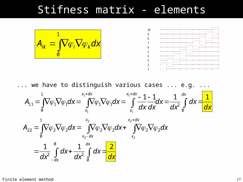
Stifness matrix - elements

dxA kiik 1

0

1

2

3

4

5

6

7

8

9

10

... we have to distinguish various cases ... e.g. ...

dxdx

dxdx

dxdxdxdxA

dxdxx

x

dxx

x

1111

0211

1

0

1111

1

1

1

1

dxdx

dxdx

dx

dxdxdxA

dx

dx

dxx

x

x

dxx

211

02

0

2

2222

1

0

2222

2

2

2

2


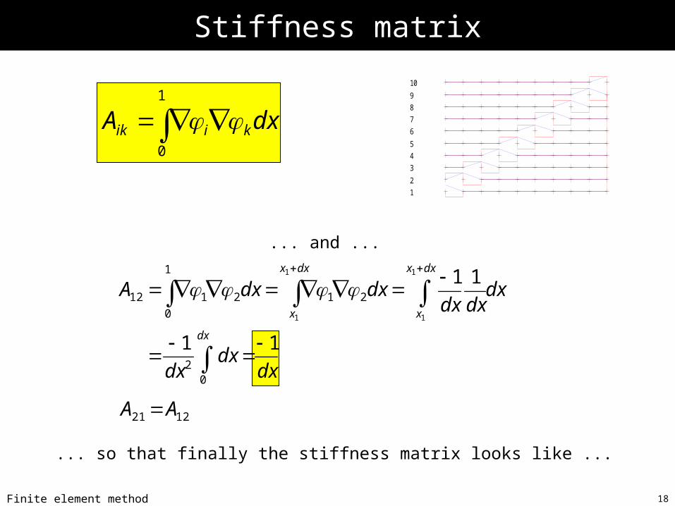
Stiffness matrix

dxA kiik 1

0

1

2

3

4

5

6

7

8

9

10

... and ...

dxdx

dx

dxdxdx

dxdxA

dx

dxx

x

dxx

x

11

11

02

21

1

0

2112

1

1

1

1

1221 AA

... and ...

... so that finally the stiffness matrix looks like ...


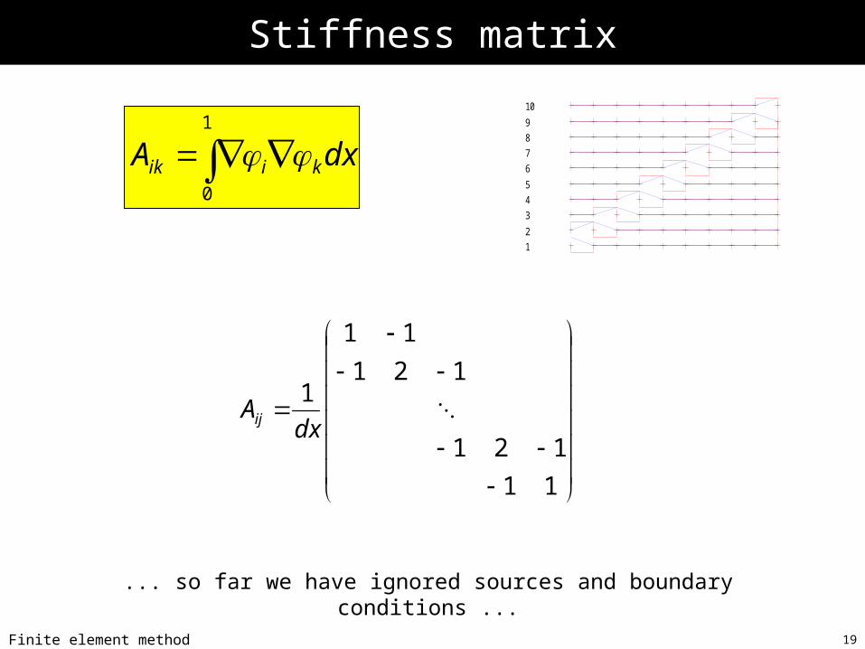
Stiffness matrix

dxA kiik 1

0

1

2

3

4

5

6

7

8

9

10

11

121

121

11

1

dxAij

... so far we have ignored sources and boundary conditions ...


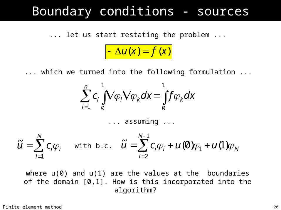
Boundary conditions - sources

... let us start restating the problem ...

)()( xfxu

... which we turned into the following formulation ...

dxfdxc kki

n

ii

1

0

1

01

... assuming ...

i

N

iicu

1

~ with b.c. Ni

N

ii uucu )1()0(~

1

1

2

where u(0) and u(1) are the values at the boundaries of the domain [0,1]. How is this incorporated into the algorithm?


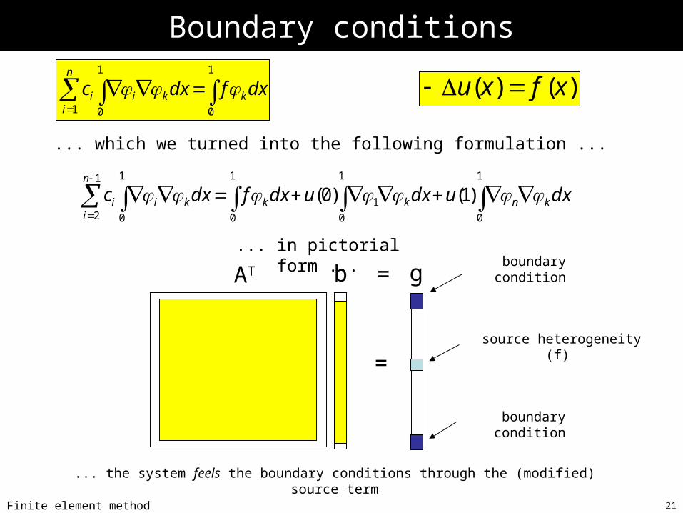
Boundary conditions

)()( xfxu

... which we turned into the following formulation ...

dxfdxc kki

n

ii

1

0

1

01

... in pictorial form ...

dxudxudxfdxc knkkki

n

ii

1

0

1

0

1

1

0

1

0

1

2

)1()0(

=

boundary condition

boundary condition

source heterogeneity (f)

... the system feels the boundary conditions through the (modified) source term

AT b = g


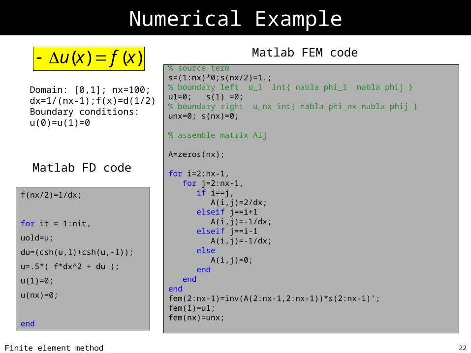
Numerical Example

)()( xfxu

Domain: [0,1]; nx=100; dx=1/(nx-1);f(x)=d(1/2)Boundary conditions:u(0)=u(1)=0

f(nx/2)=1/dx;

for it = 1:nit,

uold=u;

du=(csh(u,1)+csh(u,-1));

u=.5*( f*dx^2 + du );

u(1)=0;

u(nx)=0;

end

Matlab FD code

% source terms=(1:nx)*0;s(nx/2)=1.;% boundary left u_1 int{ nabla phi_1 nabla phij }u1=0; s(1) =0;% boundary right u_nx int{ nabla phi_nx nabla phij }unx=0; s(nx)=0;

% assemble matrix Aij

A=zeros(nx);

for i=2:nx-1, for j=2:nx-1, if i==j, A(i,j)=2/dx; elseif j==i+1 A(i,j)=-1/dx; elseif j==i-1 A(i,j)=-1/dx; else A(i,j)=0; end endendfem(2:nx-1)=inv(A(2:nx-1,2:nx-1))*s(2:nx-1)';fem(1)=u1;fem(nx)=unx;

Matlab FEM code


Regular grid

)()( xfxu

Domain: [0,1]; nx=100; dx=1/(nx-1);f(x)=d(1/2)Boundary conditions:u(0)=u(1)=0

Matlab FD code (red)

Matlab FEM code (blue)

0 0.1 0.2 0.3 0.4 0.5 0.6 0.7 0.8 0.9 10

0.05

0.1

0.15

0.2

0.25

x

u(x)

FD (red) - FEM (blue)


Regular grid - non zero b.c.

)()( xfxu

Domain: [0,1]; nx=100; dx=1/(nx-1);f(x)=d(1/2)Boundary conditions:u(0)=0.15u(1)=0.05



0 0.1 0.2 0.3 0.4 0.5 0.6 0.7 0.8 0.9 10

0.05

0.1

0.15

0.2

0.25

0.3

0.35

0.4

x

u(x)

FD (red) - FEM (blue) -> Regular grid

% Quelle

s=(1:nx)*0;s(nx/2)=1.;

% Randwert links u_1 int{ nabla phi_1 nabla phij }

u1=0.15; s(2) =u1/dx;

% Randwert links u_nx int{ nabla phi_nx nabla phij }

unx=0.05; s(nx-1)=unx/dx;


Stiffness – irregular grid

1

2

3

4

5

6

7

8

9

10

dxA kiik 1

0

2110

2

1121

1

0

2112

11

11

1

1

11

1

11

1

Ah

dxh

dxhh

dxdxA

h

hx

x

hx

x

iiii hhA

11

1

i=1 2 3 4 5 6 7 + + + + + + + h1 h2 h3 h4 h5 h6


Example

)()( xfxu

Domain: [0,1]; nx=100; dx=1/(nx-1);f(x)=d(1/2)Boundary conditions:u(0)=u0; u(1)=u1

for i=2:nx-1,

for j=2:nx-1,

if i==j,

A(i,j)=1/h(i-1)+1/h(i);

elseif i==j+1

A(i,j)=-1/h(i-1);

elseif i+1==j

A(i,j)=-1/h(i);

else

A(i,j)=0;

end

end

end

i=1 2 3 4 5 6 7 + + + + + + + h1 h2 h3 h4 h5 h6

Stiffness matrix A


Irregular grid – non zero b.c.

)()( xfxu

Domain: [0,1]; nx=100; dx=1/(nx-1);f(x)=d(1/2)Boundary conditions:u(0)=0.15u(1)=0.05



+ FEM grid points 0 0.1 0.2 0.3 0.4 0.5 0.6 0.7 0.8 0.9 10

0.05

0.1

0.15

0.2

0.25

0.3

0.35

0.4

x

u(x)

FD (red) - FEM (blue)

FEM on Chebyshev grid


Summary

In finite element analysis we approximate a function defined in a Domain D with a set of orthogonal basis functions with coefficients corresponding to the functional values at some node points.

The solution for the values at the nodes for some partial differential equations can be obtained by solving a linear system of equations involving the inversion of (sometimes sparse) matrices.

Boundary conditions are inherently satisfied with this formulation which is one of the advantages compared to finite differences.

In finite element analysis we approximate a function defined in a Domain D with a set of orthogonal basis functions with coefficients corresponding to the functional values at some node points.

The solution for the values at the nodes for some partial differential equations can be obtained by solving a linear system of equations involving the inversion of (sometimes sparse) matrices.

Boundary conditions are inherently satisfied with this formulation which is one of the advantages compared to finite differences.

Documents

Finite element method 1 Finite Elements Basic formulation Basis functions Stiffness matrix Poisson‘s equation Regular grid Boundary conditions