www.oeaw.ac.at

www.ricam.oeaw.ac.at

Inexact Data-SparseBoundary Element Tearing

and Interconnecting Methods

U. Langer, G. Of, O. Steinbach, W.Zulehner

RICAM-Report 2005-07

Inexact Data–Sparse Boundary Element Tearing

and Interconnecting Methods∗

U. Langer1,2, G. Of3, O. Steinbach4, W. Zulehner2

1Radon Institute for Computational and Applied Mathematics,

Austrian Academy of Sciences,

Altenberger Strasse 69, A–4040 Linz, Austria

2Institute for Computational Mathematics,

Johannes Kepler University of Linz,

Altenberger Strasse 69, A–4040 Linz, Austria

3Institute for Applied Analysis and Numerical Simulation,

University of Stuttgart,

Pfaffenwaldring 57, D–70569 Stuttgart, Germany

4Institute for Mathematics D, Technical University of Graz,Steyrergasse 30, A–8010 Graz, Austria

Abstract

The Boundary Element Tearing and Interconnecting (BETI) meth-ods have recently been introduced as boundary element counterparts ofthe well–established Finite Element Tearing and Interconnecting (FETI)methods. In this paper we present inexact data–sparse versions of theBETI methods which avoid the elimination of the primal unknowns anddense matrices. However, instead of symmetric and positive definite sys-tems, we finally have to solve two–fold saddle point problems. The pro-posed iterative solvers and preconditioners result in almost optimal solversthe complexity of which is proportional to the number of unknowns onthe skeleton up to some polylogarithmical factor. Moreover, the solversare robust with respect to large coefficient jumps.

1 Introduction

The Finite Element Tearing and Interconnecting (FETI) methods were intro-duced by Farhat and Roux [16] in 1991 as some kind of a dual version of theclassical iterative substructuring methods (see also the survey paper [17] by the

∗This work has been supported by the Radon Institute for Computational and AppliedMathematics (RICAM) of the Austrian Academy of Sciences, the Austrian Science Fund‘Fonds zur Forderung der wissenschaftlichen Forschung (FWF)’ under grant P14953, and theGerman Research Foundation ‘Deutsche Forschungsgemeinschaft (DFG)’ under the grant SFB404 ‘Multifield Problems in Continuum Mechanics’.

1

same authors). Meanwhile the classical FETI methods and, in particular, themore recently developed dual–primal FETI (FETI–DP) methods are well es-tablished as powerful and robust parallel solvers for large–scale finite elementequations in different fields of applications, see, e.g., [13, 14, 15, 18, 50, 52]. Thepractical success of the FETI and FETI–DP methods in real–life applicationsis supported by a rigorous theoretical analysis [7, 34, 35, 40, 41]. In particular,for second–order self–adjoint elliptic problems such as the potential equation orthe linear elasticity problem, the iteration numbers of the conjugate gradientsolver preconditioned by a properly scaled FETI preconditioner grow only likeO(1 + log(H/h)), where H and h denote the usual scaling of the subdomainsand the finite elements, respectively. Furthermore, the iteration process is in-sensitive to large jumps in the coefficients of the partial differential equations.The latter property is very important for many practical applications, e.g. inelectromagnetics, where we frequently have to solve interface problems withlarge jumps in the material coefficients. We refer the reader to the recentlypublished monograph [58] by Toselli and Widlund for more informations aboutthe analysis of FETI methods.

Recently, the Boundary Element Tearing and Interconnecting (BETI) methods[38] and the coupled BETI/FETI methods [39] were introduced. It is widelyrecognized that Boundary Element Methods (BEM) have some advantages overthe Finite Element Methods (FEM) in the treatment of unbounded regions.But we can also benefit from the BEM in some other situations like in the caseof large air subdomains without sources in electromagnetics or in the case ofmoving parts or interfaces in magnetomechanics [32]. The coupling of BEM andFEM within a domain decomposition framework seems to be very attractive (seee.g. [23] and [54]). The symmetric FEM–BEM coupling technique was origi-nally proposed by Costabel [10]. The symmetric coupling technique was thenused by Hsiao and Wendland to construct a (primal) boundary element (BE)substructuring method [31], see also [30]. Similar to the finite element substruc-turing method they eliminate the interior subdomain unknowns, which are thefluxes (tractions) in the BEM, and arrive at the symmetric and positive definiteboundary element Schur complement system that can be solved by a direct oran iterative method. For large–scale problems, a preconditioned conjugate gra-dient method should be used for efficiency reasons. However, in every iterationstep, the interior boundary element subdomain unknowns must be eliminated,i.e. a discrete single layer potential must be inverted to compute the solution ofa Dirichlet boundary value problem in every subdomain. To avoid the expensiveelimination of these interior boundary element unknowns, an inexact boundaryelement substructuring method was introduced in [36] which requires the solu-tion of a saddle point problem. The saddle point problem was solved by thepreconditioned conjugate gradient method proposed by Bramble and Pasciakfor solving system of algebraic equations with symmetric, but indefinite systemmatrices [5]. The availability of good preconditioners is very essential for theefficiency of the solver. In the inexact BE substructuring case preconditionersfor the local (subdomain) discrete single layer potential operators and for theglobal (skeleton) boundary element Schur complement are needed. The latterusually provides the global information exchange. In [9] such preconditionersare proposed and analyzed. Inexact finite element substructuring solvers wereproposed and investigated in [4, 24, 25, 26]. The first inexact FETI solver was

2

introduced and analyzed by Klawonn and Widlund in [33]. Let us mention thatinexact versions are usually more efficient than Schur complement techniques,especially in the case of sufficiently large local problems. This is typical forreally large scale problems. On PC clusters, also mid–size problems can benefitfrom inexact solution techniques.

In this paper we introduce inexact BETI methods which lead to three–fold sad-dle point problems in the first instance. However, applying an appropriate pro-jection, we can reduce the three–fold saddle point problem to a two–fold saddlepoint problem. Following the approach given in [61] we present preconditionedKrylov subspace solution methods for two–fold saddle point problems and givesharp convergence rate estimates. Similar questions arise when considering thecoupling of symmetric boundary element with mixed finite element methods[20]. The standard boundary element discretization of boundary integral op-erators with nonlocal kernel functions would lead to fully populated matrices.This is totally unacceptable for 3D boundary value problems. Indeed, alreadythe matrix–by–vector multiplication costs O(N2

h) arithmetical operations in thecase of dense matrices. Here Nh denotes the number of boundary unknownswhich is of the order O(h−(d−1)), where h denotes the usual mesh size param-eter and d is the spatial dimension (d = 2, or d = 3). The same complexityis required for the storage demand. Data–sparse approximations of the sys-tem matrix, such as multipole techniques [8, 51], panel clustering methods [28],H–matrix approaches [27] and Adaptive Cross Approximation (ACA) methods[1, 2, 3], can reduce the complexity to almost O(Nh), up to polylogarithmicperturbations, for both the arithmetical expenses and the memory demand.Here we use the Fast Multipole Method, developed in [46], in order to approxi-mate the single layer potential, the double layer potential and the hypersingularboundary integral operators which appear in the symmetric boundary integraldomain decomposition formulation. Our preconditioned Krylov subspace solversfor two–fold saddle point problems require appropriately scaled preconditionersfor the local discrete single layer potential operators, for the local boundaryelement Schur complements and for the BETI matrix in their data–sparse (fastmultipole) representations. We propose data–sparse preconditioners which re-sult in an almost optimal solver requiring O((H/h)(d−1)(1+ log(H/h))s log ε−1)arithmetical operations in a parallel regime and O((H/h)(d−1)(1 + log(H/h))2)storage units per processor, where s ∈ 3, 4, 5 depending on the quality of thepreconditioners for the local problems, and ε ∈ (0, 1) is the relative accuracyof the iteration error in a suitable norm. H and h denote the usual scalings ofthe subdomains and the boundary elements, respectively. Moreover, our solversare insensitive to large jumps in the coefficients of the potential equation thatis considered as model problem throughout the paper.

The rest of the paper is organized as follows: In Section 2, we introduce the data–sparse symmetric boundary element domain decomposition method. Section 3is devoted to the inexact BETI approach that results in a two–fold saddle–pointproblem after a suitable subspace projection. In Section 4, we present andanalyze iterative methods for solving two–fold saddle–point problems. Optimaldata–sparse boundary element preconditioners required by the solvers presentedin Section 4 are given in Section 5. This completes the solution procedure. Fi-nally, we discuss some numerical results in Section 6 and draw some conclusionsin Section 7.

3

2 Data–Sparse Boundary Element Domain

Decomposition Methods

As a model problem we consider the Dirichlet boundary value problem for thepotential equation

−div[α(x)∇u(x)] = 0 for x ∈ Ω ⊂ R3, u(x) = g(x) for x ∈ Γ = ∂Ω, (2.1)

where Ω is a bounded Lipschitz domain that is assumed to be decomposed intop non–overlapping subdomains Ωi with Lipschitz boundaries Γi = ∂Ωi. Wefurther assume that the coefficient function α(·) in the potential equation (2.1)is piecewise constant such that α(x) = αi > 0 for x ∈ Ωi, i = 1, . . . , p. Thevariational formulation of the boundary value problem (2.1) is to find u ∈ H1(Ω)with u|Γ = g such that the variational equation

p∑

i=1

αi

∫

Ωi

∇u(x)∇v(x)dx = 0 (2.2)

is satisfied for all test functions v ∈ H10 (Ω), where g is a given function from

H1/2(Γ). Applying Green’s first formula with respect to the local subdomainsΩi gives

p∑

i=1

αi

∫

Γi

∂

∂niu(x)v(x)dsx = 0 for all v ∈ H1

0 (Ω) (2.3)

due to −∆u(x) = 0 for x ∈ Ωi, where ni denotes the exterior normal vector ofΓi. For x ∈ Ωi the solution of the local Laplace equation is given by the localrepresentation formula

u(x) =

∫

Γi

U∗(x, y)∂

∂niu(x)dsx −

∫

Γi

∂

∂niU∗(x, y)u(y)dsy, (2.4)

where

U∗(x, y) =1

4π

1

|x− y|

is the fundamental solution of the Laplace operator, see, e.g., [55]. Taking thetrace and the normal derivative of the local representation formula (2.4) weobtain the Calderon system

(ui

ti

)=

(12I −Ki Vi

Di12I +K ′

i

) (ui

ti

)(2.5)

of local boundary integral equations on Γi for the Cauchy data ui = u|Γi∈

H1/2(Γi) and ti = ni · ∇u|Γi∈ H−1/2(Γi), where the local single layer potential

operator Vi : H−1/2(Γi) → H1/2(Γi), the local double layer potential operatorKi : H1/2(Γi) → H1/2(Γi), its adjoint K ′

i : H−1/2(Γi) → H−1/2(Γi), and thelocal hypersingular boundary integral operator Di : H1/2(Γi) → H−1/2(Γi) aredefined by

(Viti)(x) =

∫

Γi

U∗(x, y)ti(y)dsy,

(Kiui)(x) =

∫

Γi

∂

∂ni,yU∗(x, y)ui(y)dsy,

4

(K ′iti)(x) =

∫

Γi

∂

∂ni,xU∗(x, y)ti(y)dsy ,

(Diui)(x) = −∂

∂ni,x

∫

Γi

∂

∂ni,yU∗(x, y)ui(y)dsy,

respectively. The mapping properties of these boundary integral operators arenow well known, see, e.g., [11, 42, 55]. In particular, the local single layerpotential operators Vi are self–adjoint and H−1/2(Γi)–elliptic. The local hyper-singular operators Di are self–adjoint as well, but only positive semi–definite.Indeed, the kernel ker Di of the hypersingular operator Di is spanned by allconstant functions, i.e. ker Di = span1.Let us denote the skeleton of the domain decomposition by ΓS = ∪p

i=1Γi and theskeleton trace space by H1/2(ΓS) = v|ΓS

: v ∈ H1(Ω). Inserting the second

boundary integral equation of (2.5) into (2.3) we have to find u ∈ H1/2(ΓS)with u|Γ = g such that

p∑

i=1

αi

[〈Diu|Γi

, v|Γi〉Γi + 〈(

1

2I +K ′

i)ti, v|Γi〉Γi

]= 0 (2.6)

for all test functions v ∈ H1/20 (ΓS) = v ∈ H1/2(ΓS) : v|Γ = 0, where ti ∈

H−1/2(Γi) are the unique solutions of the local variational problems

αi

[〈Viti, wi〉Γi − 〈(

1

2I +Ki)u|Γi

, wi〉Γi

]= 0 (2.7)

for all test functions wi ∈ H−1/2(Γi), where 〈·, ·〉Γi denotes the duality pairingin H−1/2(Γi) × H1/2(Γi) that is the extension of the scalar product in L2(Γi)for i = 1, 2, . . . , p. After homogenization of the Dirichlet boundary conditionvia the ansatz u = g + u with some extension g|Γ = g and u|Γ = 0, we canrewrite (2.6) and (2.7) as mixed variational problem to find t = (t1, t2, . . . , tp) ∈T = T1 × T2 × . . . × Tp = H−1/2(Γ1) × H−1/2(Γ2) × . . . × H−1/2(Γp) and

u ∈ U = H1/20 (ΓS) such that

αi

[〈wi, Viti〉Γi − 〈wi, (

1

2I +Ki)u|Γi

〉Γi

]= αi〈wi, (

1

2I +Ki)g|Γi

〉Γi (2.8)

for all wi ∈ Ti, i = 1, 2, . . . , p, and

p∑

i=1

αi

[−〈(

1

2I +K ′

i)ti, v|Γi〉Γi − 〈Diu|Γi

, v|Γi〉Γi

]=

p∑

i=1

αi〈Dig|Γi, v|Γi

〉Γi

(2.9)for all v ∈ U . It is well known that the mixed variational problem (2.8) and(2.9) is uniquely solvable, and therefore the equivalent problem (2.6) and (2.7),too [31].

Let us now introduce the boundary element trial spaces

Uh = S1h(ΓS) = spanϕmM

m=1 ⊂ U = H1/20 (ΓS) (2.10)

andTi,h = S0

h(Γi) = spanψik

Ni

k=1 ⊂ Ti = H−1/2(Γi) (2.11)

5

spanned by continuous piecewise linear basis functions ϕm and by piecewiseconstant basis functions ψi

k with respect to a regular globally quasi–uniform

boundary element mesh Γi = ∪Ni

ℓ=1τiℓ with the average mesh size h on ΓS and

Γi, respectively. The restriction of the global trial space Uh onto the localsubdomain boundaries Γi is denoted by

Ui,h = S1h(Γi) = S1

h(ΓS)|Γi= spanϕi

mMim=1 ⊂ H

1/20 (Γi), (2.12)

where H1/20 (Γi) = v|Γi

: v ∈ H1/20 (ΓS). The Galerkin discretization of the

symmetric mixed variational formulation (2.8) and (2.9) now gives immediatelythe mixed boundary element equations to find th = (t1,h, t2,h, . . . , tp,h) ∈ Th =T1,h × T2,h × . . .× Tp,h and uh ∈ Uh such that

αi

[〈wi,h, Viti,h〉Γi − 〈wi,h, (

1

2I +Ki)uh|Γi

〉Γi

]= αi〈wi,h, (

1

2I +Ki)g|Γi

〉

(2.13)for all wi,h ∈ Ti,h, i = 1, 2, . . . , p, and

p∑

i=1

αi

[−〈(

1

2I +K ′

i)ti,h, vh|Γi〉Γi − 〈Diuh|Γi

, vh|Γi〉Γi

]=

p∑

i=1

αi〈Dig|Γi, vh|Γi

〉Γi

(2.14)for all vh ∈ Uh. Applying standard arguments, it follows that the mixed bound-ary element equations (2.13) and (2.14) admit an unique solution. Moreover,the discretization error is bounded by the approximation error,

‖u− uh‖2U + ‖t− th‖

2T ≤ c

inf

vh∈Uh

‖u− vh‖2U + inf

wh∈Th

‖t− wh‖2T

.

From the approximation properties of the boundary element trial spaces Uh andTh we then obtain the a priori error estimate

‖u− uh‖2U + ‖t− th‖

2T ≤ c h2s+1

[‖u‖2

Hs+1(ΓS) +

p∑

i=1

‖ti‖2Hs

pw(Γi)

](2.15)

for a sufficiently smooth solution (u, t) with u ∈ Hs+1(ΓS) and ti ∈ Hspw

(Γi)

and s ∈ (0, 1]. This gives an optimal convergence rate of O(h3/2), see [55]. Hereand in the following c denotes a generic constant that is always independent onthe discretization parameters.

Once the basis functions are chosen, the boundary element equations (2.13) and(2.14) are equivalent to the following system of algebraic equations to find thecoefficient vectors ti = [ti,k]Ni

k=1 ∈ RNi for i = 1, 2, . . . , p and u = [um]Mm=1 ∈ R

M

of the boundary element functions ti,h =∑Ni

k=1 ti,kψik and uh =

∑Mm=1 umϕm

as the unique solution of the Galerkin system

α1V1,h −α1K1,hR1,h

. . ....

αpVp,h −αpKp,hRp,h

−α1R⊤1,hK

⊤1,h . . . −αpR

⊤p,hK

⊤p,h −Dh

t1...tpu

=

α1g1...

αpgp

f

,

(2.16)

6

where

Dh =

p∑

i=1

αiR⊤i,hDi,hRi,h and f =

p∑

i=1

αiR⊤i,hf i

. (2.17)

The entries of the matrices Vi,h, Ki,h, Di,h and the coefficients of the right–handsides g

iand f are defined by the relations

Vi,h[ℓ, k] = 〈ψiℓ, Viψ

ik〉Γi ,

Ki,h[ℓ,m] = 〈ψiℓ, (

1

2I +Ki)ϕ

im〉Γi ,

Di,h[n,m] = 〈ϕin, Diϕ

im〉Γi

and

gi,ℓ = 〈ψiℓ, (

1

2I +Ki)g|Γi

〉Γi , fi,n = 〈Dig|Γi, ϕi

n〉Γi

for all k, ℓ = 1, . . . , Ni and m,n = 1, . . . ,Mi, respectively. The restrictionoperator Ri,h maps some global coefficient vector v ∈ R

M to the local vectorvi ∈ R

Mi containing those components of v which correspond to Γi only, i =1, 2, . . . , p. The matrices Ri,h are Boolean matrices which are sometimes alsocalled subdomain connectivity matrices.

The system matrix of (2.16) is symmetric, but indefinite. The matrices Vi,h

are symmetric and positive definite while the blocks Di,h are symmetric, but ingeneral only positive semi–definite, where the kernel is spanned by all vectorswith constant entries. Unfortunately, all matrix blocks involved in (2.16) arefully populated due to the nonlocal fundamental solution. Especially for three–dimensional boundary value problems, this fact would yield unacceptable highresources of memory and already a high complexity of a single matrix–by–vectormultiplication. Since the latter operation is the basic operation in every iterationmethod, we need some data–sparse approximation of these matrices that reducesthe quadratic complexity with respect to the number of unknowns to an almostlinear one, but without disturbing the accuracy given by the quasi–optimalestimate (2.15).

As already pointed out in the introduction there exist several possibilities offast boundary element methods to reduce the computational costs, for examplepanel clustering [28], algebraic approximation techniques such as the AdaptiveCross Approximation method [3] and hierarchical matrices [27] or wavelets [12].Here we describe the application of the fast multipole method to all the discreteboundary integral operators introduced above [46]. We will mainly use theoriginal version of the fast multipole method as described in [21, 22] but the maindifference in our version of the method, however, will be the use of reformulatedspherical harmonics [48, 59, 60].As already mentioned above, when using an iterative solver it is necessaryto perform the matrix–by–vector multiplications of the local stiffness matri-ces with given vectors efficiently. In particular, if the vectors ri

1 ∈ RNi and ri

2 ∈R

Mi are given, we need a fast computation of the matrix–by–vector productswi

1 = Vi,hri1 ∈ R

Ni , wi2 = Ki,hr

i2 ∈ R

Ni , vi1 = Di,hr

i2 ∈ R

Mi and ofvi2 = K⊤

i,hri1 ∈ R

Mi .

We begin with the local matrix–by–vector product wi1 = Vi,hr

i1 of the discrete

7

single layer potential Vi,h which reads in components

wi1,ℓ =

Ni∑

k=1

Vi,h[ℓ, k]ri1,k =

Ni∑

k=1

ri1,k

4π

∫

τ iℓ

∫

τ ik

1

|x− y|dsydsx for ℓ = 1, . . . , Ni.

As in most of the fast boundary element methods, one first substitutes the kernelfunction by an appropriate series expansion separating the integration variablesx and y from each other. The kernel of the single layer potential can be writtenin terms of Legendre polynomials,

k(x, y) =1

|x− y|=

∞∑

n=0

|x|n

|y|n+1Pn(x · y), x =

x

|x|, y =

y

|y|,

where

Pn(u) =1

2nn!

dn

dun(u2 − 1)n for |u| ≤ 1.

An approximation of the kernel function k(x, y) is then defined by truncatingthe infinite sum at at certain expansion degree ,

k(x, y) =∑

n=0

|x|n

|y|n+1Pn(x · y). (2.18)

Note that for |y| > |x| the following error estimate holds:

|k(x, y) − k(x, y)| ≤1

|y| − |x|

(|x|

|y|

)+1

. (2.19)

Since the product of the normalized integration variables x and y still appears asan argument of the Legendre polynomials in (2.18), one may rather use sphericalharmonics [29] to obtain the kernel approximation

k(x, y) =∑

n=0

n∑

m=−n

|x|n

|y|n+1Y −m

n (x)Y mn (y) =

∑

n=0

n∑

m=−n

Smn (y)Rm

n (x) (2.20)

when assuming |y| > |x|. The truncated series expansion (2.20) is the firstingredient of the fast multipole method. The second one is the use of an artificialgeometric hierarchy which is build upon the boundary elements. All boundaryelements τ i

k ⊂ Γi belong to a cluster ω0i,1 which is a box containing the whole

subdomain Ωi. The clusters of the level λ+1 are constructed by the refinementof all boxes ωλ

i,j into eight similar sub–boxes ωλ+1i,j′ . The clusters ωλ+1

i,j′ are called

the sons of the father cluster ωλi,j . This recursive process is repeated until an

maximum level L is attained. Clusters containing no boundary elements areneglected. All boundary elements τ i

kNi

k=1 are assigned to the cluster ωLi,j with

respect to their midpoints.Since the expansion (2.20) is only valid for |x| < |y|, one has to distinguish thefarfield (FF) where this expansion is admissible from the nearfield (NF) wherethe standard kernel has to be used. A cluster ωλ

j on the same level λ is called

to be in the nearfield of the cluster ωλi if the condition

distCλi , C

λj ≤ (d+ 1) maxrλ

i , rλj (2.21)

8

is satisfied with d > 1 a suitably chosen parameter. Cλi denotes the center and

rλi is the radius of the cluster ωλ

i which is determined by the cluster center andthe extension of the contained boundary elements τk ∈ ωλ

i .Hence we obtain the approximate local matrix–by–vector product

wi1,ℓ =

∑

k ∈NF(ℓ)

Vi,h[ℓ, k]ri1,k +

∑

k ∈FF(ℓ)

ri1,k

4π

∫

τℓ

∫

τk

∑

n=0

n∑

m=−n

Smn (y)Rm

n (x)dsxdsy

=∑

k ∈NF(ℓ)

Vi,h[ℓ, k]ri1,k +

∑

n=0

n∑

m=−n

∑

k ∈FF(ℓ)

ri1,k

4π

∫

τk

Rmn (x)dsx

∫

τℓ

Smn (y)dsy

for all ℓ = 1, . . . , Ni. As the farfields differ from each other for most indices ℓ, thequestion arises how to compute the coefficients of the series expansion for dif-ferent ℓ efficiently. This can be done by using the cluster hierarchy constructedabove. Starting on the finest level all coefficients for the corresponding clus-ters are computed and later translated to their common fathers on the coarserlevels up to level zero. Next, these multipole expansions are converted into lo-cal expansions in terms of their coefficients on the highest level, in which thekernel expansion is admissible. This results in an algorithm of O(Ni log2Ni)complexity. For a more detailed description of the efficient matrix–by–vectormultiplication see [46] and the references given there.In what follows we will focus on the stability and error analysis of the approx-imate matrix–by–vector product wi

1 = Vi,hri1 in the case of a fixed nearfield

parameter d > 0.

Lemma 2.1 [46, Lemma 4.1] Let = O(log h−2) and the triangulation bequasi–uniform. Then there holds the following consistency estimate for the ap-proximated single layer potential Vi,

‖(Vi − Vi)ti,h‖L2(Γi) ≤ c h2‖ti,h‖L2(Γi) for all ti,h ∈ S0h(Γi) ⊂ L2(Γi).

From the previous lemma and using the inverse inequality it is possible to choosethe expansion degree = O(logNi) such that the approximate single layer

potential Vi,h is S0h(Γi)–elliptic,

〈Vi,hwi,h, wi,h〉Γi ≥ ceVi1 ‖wi,h‖

2H−1/2(Γ) for all wi,h ∈ S0

h(Γi).

The multipole expansion of the double layer potential operator Ki can be com-puted by applying the normal derivative to the expansion (2.20) of the singlelayer potential Vi. In the case of the adjoint double layer potential K ′

i, thenormal derivative has to be applied to the coefficients in the evaluation of theexpansions. Therefore the transposition property between the Galerkin matri-ces of the the double layer potential and its adjoint operator will be maintainedif the same expansion degree p is chosen for both. As for the approximate singlelayer potential Vi,h corresponding error estimates follow, see [46, Lemma 4.3,Lemma 4.4].The hypersingular boundary integral operator Di is treated via integration byparts [44]. The bilinear form of the hypersingular integral operator Di can bewritten as sum of bilinear forms of the single layer potential Vi,

〈Diui, vi〉Γi =3∑

k=1

〈Vicurl|Γiui|k, curl|Γi

vi|k〉Γi ,

9

with the surface curl curl|Γiui(x) = nx×∇u∗i,Γi

(x) defined for a constant exten-sion u∗i|Γi

of u(x) along the normal nx into a small neighborhood of Γi. In the

case of piecewise linear, continuous basis functions ϕim(x) and plane triangles as

boundary elements, the vector curlΓiϕi

m(x) is piecewise constant and constanton each boundary element. Therefore the Galerkin matrix of the single layerpotential Vi for piecewise constant basis functions ψi

k can be reused here leadingto the approximate bilinear form

〈Di,hui,h, vi,h〉Γi =

3∑

k=1

〈Vi,hcurl|Γiui,h|k, curl|Γi

vi,h|k〉Γi . (2.22)

The stability and error analysis for the approximation Di,h then follows as forthe approximate single layer potential.

Using the fast multipole approximations for the application of the discreteboundary integral operators, instead of (2.16) we have to solve the perturbedlinear system

α1V1,h −α1K1,hR1,h

. . ....

αpVp,h −αpKp,hRp,h

−α1R⊤1,hK

⊤1,h . . . −αpR

⊤p,hK

⊤p,h −Dh

t1...

tpu

=

α1g1...

αpgp

f

.

(2.23)As for the symmetric boundary integral formulation considered in [46, Theorem4.1] there follows the unique solvability of (2.23) as well as the quasi–optimalerror estimate

‖u− uh‖2U + ‖t− th‖

2T ≤ c h2s+1

[‖u‖2

Hs+1(ΓS) +

p∑

i=1

‖ti‖2Hs

pw(Γi)

](2.24)

for the associated approximate solutions th ∈ Th and uh ∈ Uh when assuming = O(logNi) and smooth solutions as in (2.15), i.e., s ∈ (0, 1]. Hence wecan ensure the same asymptotic behavior as for the solution of the standardGalerkin boundary element method.A standard approach to solve the linear system (2.23) is to consider its Schurcomplement system

p∑

i=1

αiR⊤i,h

[Di,h + K⊤

i,hV−1i,h Ki,h

]Ri,hu = −

p∑

i=1

αiR⊤i,h

[f

i+ K⊤

i,hV−1i,h gi

]

(2.25)with the symmetric and positive definite system matrix

Sh =

p∑

i=1

αiR⊤i,hSi,hRi,h, Si,h = Di,h + K⊤

i,hV−1i,h Ki,h.

The linear system (2.25) can be solved by a conjugate gradient scheme wherethe application of a possible preconditioner is given by

C−1S =

p∑

i=1

1

αiR⊤

i,hVi,hRi,h (2.26)

10

and Vi,h is the single layer potential discretized by piecewise linear continuousbasis functions and approximated by means of a fast multipole method. Notethat each application of the discrete Steklov–Poincare operators Si,h withinone step of the conjugate gradient scheme requires one inversion of the discretesingle layer potential Vi,h which can be realized by an interior conjugate gradientscheme.

3 Inexact BETI Methods

In order to avoid assembled matrices and vectors, we tear the global potentialvector u on the subdomain boundaries Γi by introducing the individual localunknowns

ui = Ri,hu. (3.1)

Conversely, the global continuity of the potentials is enforced by the constraints

p∑

i=1

Biui = 0 (3.2)

interconnecting the local potential vectors across the subdomain boundaries.Each row of the matrix B = (B1, . . . , Bp) is connected with a pair of match-ing nodes across the subdomain boundaries. The entries of such a row are 1and −1 for the indices corresponding to the matching nodes on the interface(coupling boundaries) ΓC = ΓS \ Γ and 0 otherwise. Therefore, (3.2) impliesthat the corresponding boundary element functions ui,h are continuous acrossthe interface ΓC , i.e. ui,h = uj,h on Γi ∩ Γj 6= ∅. We assume here that thenumber of constraints at some matching node is equal to the number of match-ing subdomains minus one. This method of a minimal number of constraintsrespectively multipliers is called non–redundant, see, e.g., [34] for the use ofredundant constraints.By introducing Lagrange multipliers λ ∈ R

L the linear system (2.23) is equiva-lent to

0BBBBBBBBBBBB@

α1eV1,h −α1

eK1,h

. . .. . .

αpeVp,h −αp

eKp,h

−α1eK⊤

1,h−α1

eD⊤

1,hB⊤

1

. . .. . .

.

..

−αpeK⊤

p,h−αp

eDi,h B⊤p

B1 . . . Bp

1CCCCCCCCCCCCA

0BBBBBBBBBBB@

et1

...etpeu1

...eup

λ

1CCCCCCCCCCCA

=

0BBBBBBBBBBBB@

α1g1

...αpg

p

α1f1

..

.αpf

p

0

1CCCCCCCCCCCCA

.

Setting V = diag(αiVi,h), K = diag(αiKi,h), D = diag(αiDi,h) as well asB = (B1, . . . , Bp) we have to solve the two–fold saddle point problem

V −K 0−K⊤ −D B⊤

0 B 0

tuλ

=

gf0

(3.3)

when ordering the vectors in an appropriate way. The matrix Di,h is symmetricand positive definite if and only if the corresponding subdomain Ωi is a so–called

11

non–floating subdomain. A subdomain Ωi is called floating if the subdomainboundary Γi does not touch the Dirichlet boundary part ΓD that is Γ for ourmodel problem (2.1). Otherwise the subdomain is called non–floating. For a

floating subdomain Ωi the kernel of the matrix Di,h is spanned by the vector

ei = (1, . . . , 1)⊤ ∈ RMi , i.e. ker Di,h = spanei. Let us assume for simplicity

that the first q (q < p) subdomains are floating and the remaining subdomainsare non–floating. The case q = 0 (no floating subdomains) is trivial and does

not need any discussion. In order to avoid singular block entries Di,h and,

therefore, singular Schur complements Si,h = αi(Di,h + K⊤i,hV

−1i,h Ki,h) for the

floating subdomains, we replace the singular blocks Di,h by the regularized

matrices Di,h + βieie⊤i with appropriately choosen positive constants βi for

i = 1, . . . , q. We mention that

Ki,hei = 0 for i = 1, . . . , q. (3.4)

Let us denote the unique solutions of the regularized equations

αi(Di,h + βieie⊤i )vi = −αif i

+Biλ− αiK⊤i,hti (3.5)

by vi, i = 1, . . . , q. If the right hand side of (3.5) fulfills the solvability conditionsfor the original equations without the regularization term,

e⊤i (−αif i+Biλ− αiK

⊤i,hti) = e⊤i (−αif i

+Biλ) = 0, (3.6)

then the solution vi of (3.5) is orthogonal to ker Di,h, i.e.

e⊤i vi = 0. (3.7)

Now the solution u = (u1, . . . , up)⊤ of the original system (3.3) can be recovered

by the formulaeui = vi + γiei, (3.8)

with γi = 0 for i = q + 1, . . . , p and appropriately chosen γi for i = 1, . . . , q.Taking into account (3.4)–(3.8), we easily observe that the unique solution t ∈R

M , v ∈ RN , λ ∈ R

L and γ ∈ Rq of the three–fold saddle point problem

V −K 0 0−K⊤ −D B⊤ 0

0 B 0 G0 0 G⊤ 0

tvλγ

=

gf0e

(3.9)

immediately yields the solution (t, u, λ) of the two–fold saddle point problem(3.3), where now D is symmetric and positive definite since we replaced the

singular blocks Dj,h by the regularized ones for the floating subdomains. Thelast equation in (3.9) is nothing but the solvability condition (3.6). Note thatthe L× q matrix G and the vector e ∈ R

q are defined by the relations

G = (B1e1, . . . , Bqe1) and e = (e⊤1 f1, . . . , e⊤q fq

)⊤. (3.10)

Now we use a subspace projection in order to separate the determination of γfrom the determination of the rest of the unknowns in (3.9). Thus, we introducethe orthogonal projection

P = I −G(G⊤G)−1G⊤ (3.11)

12

from the space Λ := RM onto the subspace Λ0 = kerG⊤ = (rangeG)⊥ with

respect to the scalar product (·, ·) = (·, ·)Λ = (·, ·)RM . We mention that in thecase of large jumps in the coefficients of the PDE the scalar product in Λ hasto be changed according to the proposal made in [34], see also [7] and [58]. Ofcourse, the change of the scalar product changes the orthoprojection P too.Since PG = 0, the application of P to the third equation of (3.9) gives PBv = 0that excludes γ from the first three equations of (3.9). Let us represent λ in theform

λ = T0λ0 + λe (3.12)

with known λe = G(G⊤G)−1e ∈ (kerG⊤)⊥ = rangeG, fulfilling the constraintsG⊤λe = e, and unknown T0λ0 ∈ kerG⊤, i.e. G⊤λ0 = 0, where λ0 ∈ R

L0 andL0 = dim Λ0. The columns of T0 span a basis of Λ0. We refer to Remark 3.1 forthe practical implementation of the determination of λ0 via subspace iteration.Now we can define t, v and λ0 from the two–fold saddle point problem

V −K 0

−K⊤ −D B⊤P⊤T0

0 T⊤0 PB 0

tvλ0

=

gd0

, (3.13)

where here d = f −B⊤λe. Once the vectors t, v and λ0 are defined from (3.13),we get λ from (3.12), γ from the third equation of (3.9), i.e.

γ = −(G⊤G)−1G⊤Bv, (3.14)

and, finally, u from (3.8).

Remark 3.1 We mention that the iteration updates for λ completely life inthe subspace Λ0 if the initial guess is chosen as λe. Therefore, a basis of Λ0,forming the columns of T0, is not explicitly needed in the computation (see alsoAlgorithm 5.1 in Section 5).

Since V = diag(αiVi,h) is block diagonal and therefore easily invertible we alsomay eliminate the vector t in (3.13) to obtain

(S −B⊤P⊤T0

T⊤0 PB 0

) (vλ0

)=

(−d− V −1g

0

)(3.15)

withS = diag(αiSi,h), Si,h = Di,h + K⊤

i,hV−1i,h Ki,h.

Eliminating v we have to solve the Schur complement system of (3.15),

Fλ0 = T⊤0 PBS

−1B⊤P⊤T0λ0 = T⊤0 PBS

−1[d+ V −1g]. (3.16)

Appropriate strategies to solve (3.16) were considered in [38]; another choiceis the application of a Bramble–Pasciak conjugate gradient scheme to the one–fold saddle point problem (3.15). Note that appropriate preconditioners forboth methods coincide with preconditioners already needed for solving (3.13),see Section 5.

13

4 Solution of Two–fold Saddle Point Problems

In this section we construct and analyze preconditioned CG–like iterative meth-ods for solving two–fold saddle point problems possessing exactly the structureand the properties of the two–fold saddle point problem (3.13), namely

A1 B⊤

1 0B1 −A2 B⊤

2

0 B2 0

x1

x2

x3

=

b1b2b3

, (4.1)

where S1 = A1, A2, S2 = A2 + B1A−11 B⊤

1 and S3 = B2S−12 B⊤

2 are symmetricand positive definite. It is easy to see that the system matrix

K3 =

A1 B⊤1 0

B1 −A2 B⊤2

0 B2 0

of (4.1) possesses a block LU–decomposition:

K3 = L3 U3 (4.2)

with

L3 =

S1

B1 −S2

B2 −S3

and U3 =

I S−1

1 BT1

I −S−12 BT

2

I

The factor L3 motivates the following construction of a preconditioner L3: Westart by replacing S1, S2 and S3 by preconditioners S1, S2 and S3. Additionally,we introduce two scaling factors. First the left upper block is premultiplied bysome factor τ1 > 0 leading to a 2–by–2 sub matrix

L2 =

(τ1 S1

B1 −S2

).

We end up with the final form of the preconditioner by premultiplying this submatrix by some second scaling factor τ2 > 0:

L3 =

(τ2 L2

B2E2 S3

)=

τ2τ1 S1

τ2 B1 −τ2 S2

B2 S3

with E2 =(0 I

). Now we have:

Theorem 4.1 If the parameter τ1 is chosen such that

0 < τ1 < λmin(S−11 A1)

then the matrix L−12 K2 is symmetric and positive definite in the scalar product

(u, v)2 = (D2u, v)ℓ2 with

K2 =

(A1 BT

1

B1 −A2

)and D2 =

(A1 − τ1 S1

S2

).

14

If, additionally, the parameter τ2 is chosen such that

0 < τ2 < λmin(L−12 K2)

then the matrix L−13 K3 is symmetric and positive definite in the scalar product

(u, v)3 = (D3u, v)ℓ2 with

D3 =

(D2(L

−12 K2 − τ2 I) 0

0 S3

).

For the proof, see [62].This theorem shows that we can apply the standard conjugate gradient methodin the scalar product (u, v)3 = (D3u, v)ℓ2 to the preconditioned system

L−13 K3 x = L−1

3 b,

which is equivalent to (4.1), with x = (x1, x2, x3)⊤ and b = (b1, b2, b3)

⊤. Thenwe obtain the following well–known error estimate for the n–th iterate x(n) ofthe conjugate gradient method in the corresponding energy norm:

‖x− x(n)‖D3L−1

3K3

≤2qn

1 + q2n‖x− x(0)‖D3L

−1

3K3

with q = (√κ(L−1

3 K3) − 1)/(√κ(L−1

3 K3) + 1), where κ(L−13 K3) denotes the

relative condition number: κ(L−13 K3) = λmax(L

−13 K3)/λmin(L

−13 K3).

The next theorem provides an estimate for this relative condition number de-pending on the quality of the preconditioners for the Schur complements:

Theorem 4.2 If

σ1 S1 ≤ S1 ≤ σ1 S1, σ2 S2 ≤ S2 ≤ σ2 S2, σ3 S3 ≤ S3 ≤ σ3 S3

and the parameters τ1 and τ2 are chosen such that

τ1 < λ1, τ2 < λ2

then the matrices L−12 K2 and L−1

3 K3 are symmetric and positive definite withrespect to the scalar products (., .)2 and (., .)3 and

λmin(L−13 K3) ≥ λ3, λmax(L

−13 K3) ≤ λ3 and κ(L−1

3 K3) ≤λ3

λ3

,

where λ1 = σ1,

λi+1 =1

2τi

(σi(σi+1 + 1) −

√σ2

i (σi+1 + 1)2 − 4τiσiσi+1

)for i = 1, 2

and λ3 is the largest positive zero of the rational function

θ3(λ) = −λ

σ3+

1 − λ

−τ2λ

σ2+

1 − τ2λ

−τ1τ2λ

σ1+ 1

.

15

For the proof see [62].

Remark 4.1 1. It is necessary to keep the parameters τ1 and τ2 below thelimiting values λ1 and λ2 in order to guarantee a well-defined scalar prod-uct (u, v)3. On the other hand, the closer these parameters are to theirlimiting values, the better it is, i.e.: the smaller is the upper bound λ3/λ3

for the relative condition number.

2. If the parameters τ1 and τ2 are chosen close to their limiting values λ1

and λ2 in the sense:

λi

τi= O(1) for i = 1, 2,

and if the spectral bounds are reasonably scaled:

1 + σiσi ≤ O(σi) for i = 1, 2, 3,

it can be shown, see [62], that

λ3

λ3

= O

(σ1

σ1

σ2

σ2

σ3

σ3

).

5 Data–Sparse BEM Preconditioners

As seen in the previous section we need to have appropriate efficient precondi-tioners for the local discrete single layer potentials Vi,h, for the local discrete

Schur complements Si,h as well as for the assembled BETI Schur complementF , respectively.

Since the bilinear form of the local approximate discrete single layer potentialVi,h is spectrally equivalent to the Galerkin matrix Vi,h and therefore to theH−1/2(Γi)–norm, we may use any multilevel representation of an equivalentnorm in H−1/2(Γi), [19, 47]. A suitable multilevel [6] operator is defined by

A−1/2i wi,h =

J∑

j=0

hi,j(Qi,j −Qi,j−1)wi,h

for wi,h ∈ Ti,h = Ti,J where Ti,0 ⊂ Ti,1 ⊂ . . . ⊂ Ti,J = Ti,h ⊂ . . . is a nestedsequence of boundary element spaces of piecewise constant basis functions withrelated mesh sizes hi,j = 1

2hi,j−1. Moreover, Qi,j : L2(Γi) → Ti,j is the L2

Galerkin projection onto Ti,j .

Lemma 5.1 [47, Theorem 2] The hold the spectral equivalence inequalities

cVi1 J−2 〈A

−1/2i wi,h, wi,h〉Γi ≤ (Vi,hwi, wi) ≤ cVi

2 〈A−1/2i wi,h, wi,h〉Γi

for all wi,h ∈ Ti,J = Ti,h with J = O(1 + | logH/h|).

Note that in the case of piecewise constant basis functions the L2 projectionsQi,jwi can be computed directly by inverting diagonal matrices.

16

The crucial issue in the multilevel preconditioning approach is the availabilityof the nested hierarchy of boundary element spaces Ti,j . Starting from a coarsemesh with an associated space Ti,0 one can define all boundary element spacesTi,j and therefore Ti,h = Ti,J by a recursive refinement procedure. Instead ofthis more academic situation we now consider the case where already the bound-ary element space Ti,h = Ti,J is given and no further refinement is applicable.In this case we have to construct an artificial mesh hierarchy to define an appro-priate multilevel operator. For this again we will use ideas from fast boundaryelement methods, in particular we will introduce an appropriate clustering hier-archy of all boundary elements as it is used in the fast multipole method itself.Using a recursive bisection algorithm all boundary elements τ i

k belonging to asubdomain boundary Γi can be clustered hierarchically. Since the boundaryelement spaces Ti,h are spanned by piecewise constant basis functions, one candefine corresponding piecewise constant coarse grid functions with respect tothe cluster of underlying boundary elements. This results in an artificial hier-archy of piecewise constant trial spaces which can be used for the definition ofthe multilevel operator for preconditioning [53].

To construct preconditioning matrices CSi for the local discrete Schur comple-

ment matrices Si,h = Di,h + K⊤i,hV

−1i,h Ki,h we will apply the concept of bound-

ary integral operators of the opposite order [56]. Based on the local trial spaceUi,h = S1

h(Γi) of piecewise linear basis functions ϕim as used for the Galerkin dis-

cretization of the local hypersingular boundary integral operators Di we definethe Galerkin matrices

Vi,h[n,m] = 〈ϕin, V ϕ

im〉Γi , Mi,h[n,m] = 〈ϕi

n, ϕim〉Γi

for m,n = 1, . . . ,Mi and the application of the resulting preconditioning matrixis given by

C−1Si

= M−1i,h Vi,hM

−1i,h for i = 1, . . . , p. (5.1)

When the application of the discrete single layer potential Vi,h is realized byusing a fast multipole method as described in Section 2 this results in an ap-proximated preconditioning matrix CSi .

Lemma 5.2 In the case of a non–floating subdomain Ωi with Γi ∩ Γ 6= ∅ therehold the spectral equivalence inequalities

cSi1 [1 + log2H/h]−1 (CSivi, vi) ≤ (Si,hvi, vi) ≤ cSi

2 (CSivi, vi) (5.2)

for all vi ∈ RMi while for a floating subdomain Ωi with Γi ∩ Γ = ∅ the spectral

equivalence inequalities

cSi1 (CSivi, vi) ≤ (Si,hvi, vi) ≤ cSi

2 (CSivi, vi) (5.3)

for all vi ∈ RMi with e⊤i vi = 0 are valid where cSi

1 and cSi2 are some positive

constants independent of h and H.

Proof. Since the approximated discrete single layer potential Vi,h is spectrallyequivalent to the Galerkin matrix Vi,h and therefore positive definite, and usingthe representation (2.22) of the approximate hypersingular boundary integral

17

operator Di we first conclude

(Si,hvi, vi) ≥ (Di,hvi, vi) + (V −1i,h Ki,hvi, Ki,hvi) ≥ (Di,hvi, vi)

=

3∑

k=1

〈Vi,hcurl|Γivi,h|k, curl|Γi

vi,h|k〉Γi

≥ c3∑

k=1

〈Vicurl|Γivi,h|k, curl|Γi

vi,h|k〉Γi = c (Di,hvi, vi)

for all vi ∈ RMi . The approximate discrete Steklov–Poincare operator Si,h is

bounded above [9, 54], i.e.

(Si,hvi, vi) ≤ (Si,hvi, vi) = 〈Sivi,h, vi,h〉Γi ≤ c 〈Divi,h, vi,h〉Γi = c (Di,hvi, vi)

holds for all vi ∈ RMi . Hence, to find a preconditioner for Si,h it is sufficient to

find a preconditioner for the discrete hypersingular integral operator Di,h. Inthe case of a floating subdomain Ωi with Γi ∩Γ = ∅ the preconditioning matrixCSi = Mi,hVi,hMi,h is spectrally equivalent to the discrete hypersingular integraloperator Di,h [56], and since the multipole approximation of Vi,h is spectrally

equivalent to Vi,h the same is true for the approximate preconditioner CSi , seealso [45]. Hence we obtain the spectral equivalence inequalities (5.3).When the subdomain Ωi is a non–floating subdomain with Γi∩Γ 6= ∅ we have touse the trial space Ui,h ⊂ H1/2(Γi\(Γ ∩ Γi)) of piecewise linear basis functionsvanishing on the Dirichlet boundary Γ. Due to the mapping properties of theboundary integral operators

Di : H1/2(Γi\(Γ ∩ Γi)) → H−1/2(Γi\(Γ ∩ Γi)),

Vi : H−1/2(Γi\(Γ ∩ Γi)) → H1/2(Γi\(Γ ∩ Γi))

we have to consider the discrete embedding

‖vh‖2H1/2(Γi\(Γ∩Γi))

≤ c [1 + log2H/h] ‖vh‖2eH1/2(Γi\(Γ∩Γi))

for vh ∈ Ui,h yielding the spectral equivalence inequalities (5.2), see [43] togetherwith an appropriate scaling argument.

We finally have to describe a suitable preconditioning matrix for the BETI Schurcomplement

F =

q∑

i=1

1

αiBi[Si,h + βieie

⊤i ]−1B⊤

i +

p∑

i=q+1

BiS−1i,hB

⊤i .

Following [38] we can define the scaled sparse hypersingular BETI preconditioner

C−1F = (BC−1

α BT )−1BC−1α DhC

−1α BT (BC−1

α B⊤)−1. (5.4)

Lemma 5.3 [38, Theorem 3.2] For the scaled sparse hypersingular BETI pre-conditioner (5.4), the condition estimate

κ(PC−1F PTPTFP ) ≤ c

(1 + log

H

h

)2

(5.5)

holds, where the positive constant c is independent of h, H, p and the αi’s(coefficient jumps).

18

Combining Theorem 4.2 with the results of Lemmata 5.1–5.3 and taking intoaccount the complexity estimate for the fast multipole method we can finallyarrive at our main theorem.

Theorem 5.1 If the two–fold saddle point problem (3.13) is solved by the 2SPCGalgorithm where the preconditioner is built from the block preconditioners CV ,CS and CF , respectively, then not more than I(ε) = O((1 + log(H/h))3 log ε−1)iterations and ops(ε) = O((H/h)2(1 + log(H/h))5 log ε−1) arithmetical opera-tions in a parallel regime are required in order to reduce the initial error bythe factor ε ∈ (0, 1) in a parallel regime. The number of iterations I(ε) isrobust with respect to the jumps in the coefficients. Moreover, not more thanO((H/h)2(1 + log(H/h))2) storage units are needed per processor.

Note that the complexity estimates given in Theorem 5.1 take not into accountthe costs for the projection (3.11) that involves the global information exchange.

Remark 5.1 If we use optimal preconditioners CVi for the local single layer

potentials Vi,h and CSi for the local boundary element Schur complements Si,h,then the number of iteration I(ε) of our 2SPCG solver would behave likeO((1 + log(H/h)) log ε−1), whereas the arithmetical complexity would decreasefrom O((H/h)2(1 + log(H/h))5 log ε−1) to O((H/h)2(1 + log(H/h))3 log ε−1).Such preconditioners are available, see, e.g., [37, 49, 56, 57]. If we convertthe non–floating subdomains having a Dirichlet boundary part to floating subdo-mains by including the Dirichlet boundary condition into the constraints, thenthe data–sparse opposite order preconditioners Si,h given above is optimal.

Applying the 2SPCG introduced in Section 4 to our two–fold saddle point prob-lem (3.13) with the preconditioners presented above and taking into accountRemark 3.1, we obtain a subspace iteration version of the 2SPCG that can berewritten in following algorithmic form:Note that for an efficient implementation, the application of D3L

−13 and D−1

3

have to be concatenated, see [55, 62]. Here, we have used the notations of Section4 for the matrix in (3.13) and a vector x = (x1, x2, x3)

T , where xi correspondsto the i-th block of the system (3.13).Algorithm 5.1 was used in our numerical experiments the results of which aregiven in the next section.

6 Numerical Results

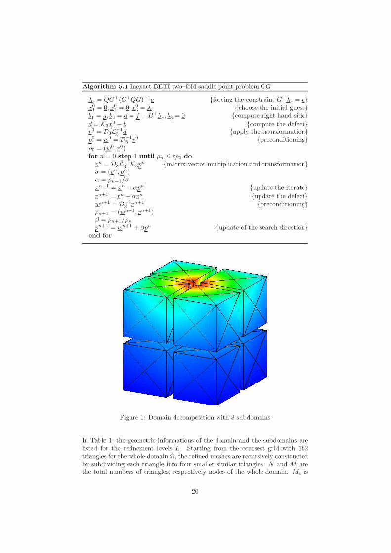
For the numerical examples we consider the unit cube which is subdivided intoeight similar subdomains as shown in Figure 1. The given Dirichlet data g(x)is chosen as the trace of a regular solution of the boundary value problem (2.1).This allows to check the convergence of the computed numerical solution to theexact one.

19

Algorithm 5.1 Inexact BETI two–fold saddle point problem CG

λe = QG⊤(G⊤QG)−1e forcing the constraint G⊤λe = ex0

1 = 0, x02 = 0, x0

3 = λe choose the initial guessb1 = g, b2 = d = f −B⊤λe, b3 = 0 compute right hand side

d = K3x0 − b compute the defect

r0 = D3L−13 d apply the transformation

p0 = w0 = D−13 r0 preconditioning

ρ0 = (w0, r0)for n = 0 step 1 until ρn ≤ ερ0 do

vn = D3L−13 K3p

n matrix vector multiplication and transformationσ = (vn, pn)α = ρn+1/σxn+1 = xn − αpn update the iterate

rn+1 = rn − αvn update the defectwn+1 = D−1

3 rn+1 preconditioningρn+1 = (wn+1, rn+1)β = ρn+1/ρn

pn+1 = wn+1 + βpn update of the search directionend for

Figure 1: Domain decomposition with 8 subdomains

In Table 1, the geometric informations of the domain and the subdomains arelisted for the refinement levels L. Starting from the coarsest grid with 192triangles for the whole domain Ω, the refined meshes are recursively constructedby subdividing each triangle into four smaller similar triangles. N and M arethe total numbers of triangles, respectively nodes of the whole domain. Mc is

20

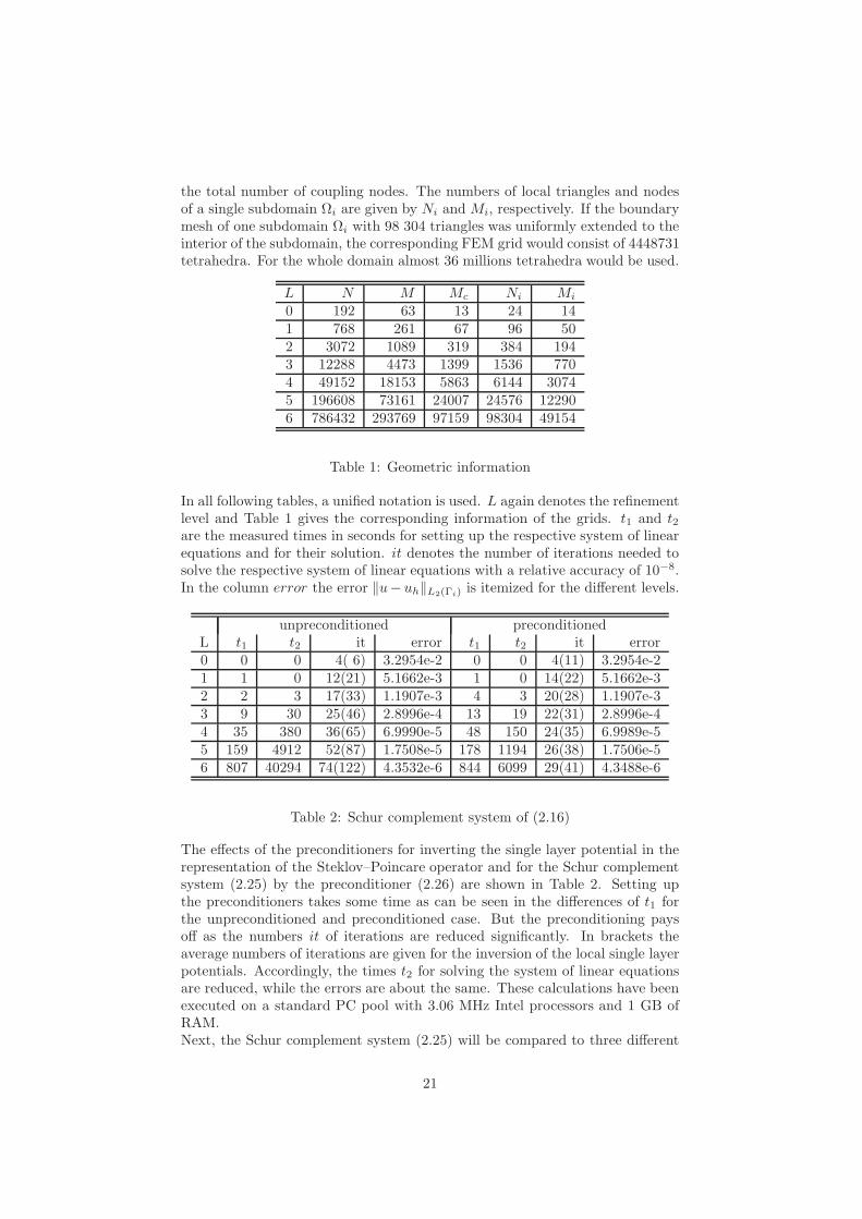
the total number of coupling nodes. The numbers of local triangles and nodesof a single subdomain Ωi are given by Ni and Mi, respectively. If the boundarymesh of one subdomain Ωi with 98 304 triangles was uniformly extended to theinterior of the subdomain, the corresponding FEM grid would consist of 4448731tetrahedra. For the whole domain almost 36 millions tetrahedra would be used.

L N M Mc Ni Mi

0 192 63 13 24 141 768 261 67 96 502 3072 1089 319 384 1943 12288 4473 1399 1536 7704 49152 18153 5863 6144 30745 196608 73161 24007 24576 122906 786432 293769 97159 98304 49154

Table 1: Geometric information

In all following tables, a unified notation is used. L again denotes the refinementlevel and Table 1 gives the corresponding information of the grids. t1 and t2are the measured times in seconds for setting up the respective system of linearequations and for their solution. it denotes the number of iterations needed tosolve the respective system of linear equations with a relative accuracy of 10−8.In the column error the error ‖u− uh‖L2(Γi) is itemized for the different levels.

unpreconditioned preconditionedL t1 t2 it error t1 t2 it error0 0 0 4( 6) 3.2954e-2 0 0 4(11) 3.2954e-21 1 0 12(21) 5.1662e-3 1 0 14(22) 5.1662e-32 2 3 17(33) 1.1907e-3 4 3 20(28) 1.1907e-33 9 30 25(46) 2.8996e-4 13 19 22(31) 2.8996e-44 35 380 36(65) 6.9990e-5 48 150 24(35) 6.9989e-55 159 4912 52(87) 1.7508e-5 178 1194 26(38) 1.7506e-56 807 40294 74(122) 4.3532e-6 844 6099 29(41) 4.3488e-6

Table 2: Schur complement system of (2.16)

The effects of the preconditioners for inverting the single layer potential in therepresentation of the Steklov–Poincare operator and for the Schur complementsystem (2.25) by the preconditioner (2.26) are shown in Table 2. Setting upthe preconditioners takes some time as can be seen in the differences of t1 forthe unpreconditioned and preconditioned case. But the preconditioning paysoff as the numbers it of iterations are reduced significantly. In brackets theaverage numbers of iterations are given for the inversion of the local single layerpotentials. Accordingly, the times t2 for solving the system of linear equationsare reduced, while the errors are about the same. These calculations have beenexecuted on a standard PC pool with 3.06 MHz Intel processors and 1 GB ofRAM.Next, the Schur complement system (2.25) will be compared to three different

21

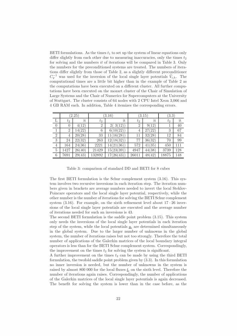
BETI formulations. As the times t1 to set up the system of linear equations onlydiffer slightly from each other due to measuring inaccuracies, only the times t2for solving and the numbers it of iterations will be compared in Table 3. Onlythe numbers for the preconditioned systems are treated. The numbers of itera-tions differ slightly from those of Table 2, as a slightly different preconditionerC−1

V was used for the inversion of the local single layer potentials Vi,h. Thecomputational times are a little bit higher than in the example of Table 2 asthe computations have been executed on a different cluster. All further compu-tations have been executed on the mozart cluster of the Chair of Simulation ofLarge Systems and the Chair of Numerics for Supercomputers at the Universityof Stuttgart. The cluster consists of 64 nodes with 2 CPU Intel Xeon 3,066 and4 GB RAM each. In addition, Table 4 itemizes the corresponding errors.

(2.25) (3.16) (3.15) (3.3)L t2 it t2 it t2 it t2 it0 0 4(12) 2 2( 3(12)) 2 9(12) 1 401 2 14(22) 6 6(10(22)) 4 27(22) 3 672 4 20(28) 33 11(16(28)) 11 32(28) 12 843 24 22(32) 263 12(18(32)) 77 36(32) 70 994 164 24(36) 2221 14(21(36)) 572 41(35) 450 1115 1427 26(40) 21429 15(23(39)) 4947 44(38) 3739 1286 7691 29(43) 132892 17(26(43)) 26011 48(42) 18875 148

Table 3: comparison of standard DD and BETI for 8 cubes

The first BETI formulation is the Schur complement system (3.16). This sys-tem involves two recursive inversions in each iteration step. The iteration num-bers given in brackets are average numbers needed to invert the local Steklov-Poincare operators and the local single layer potential, respectively, while theother number is the number of iterations for solving the BETI Schur complementsystem (3.16). For example, on the sixth refinement level about 17 · 26 inver-sions of the local single layer potentials are executed and the average numberof iterations needed for such an inversions is 43.The second BETI formulation is the saddle point problem (3.15). This systemonly needs the inversions of the local single layer potentials in each iterationstep of the system, while the local potentials ui are determined simultaneouslyin the global system. Due to the larger number of unknowns in the globalsystem, the number of iterations raises but not too strongly. Therefore the totalnumber of applications of the Galerkin matrices of the local boundary integraloperators is less than for the BETI Schur complement system. Correspondingly,the improvement on the times t2 for solving the system is significant.A further improvement on the times t2 can be made by using the third BETIformulation, the twofold saddle point problem given by (3.3). In this formulationno inner inversion is needed, but the number of unknowns in the system israised by almost 800 000 for the local fluxes ti on the sixth level. Therefore thenumber of iterations again raises. Correspondingly, the number of applicationsof the Galerkin matrices of the local single layer potentials is again decreased.The benefit for solving the system is lower than in the case before, as the

22

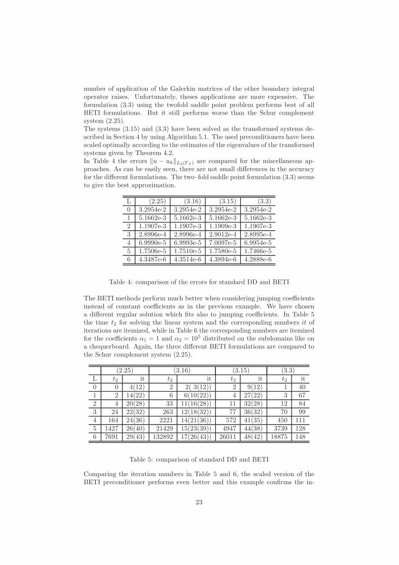
number of application of the Galerkin matrices of the other boundary integraloperator raises. Unfortunately, theses applications are more expensive. Theformulation (3.3) using the twofold saddle point problem performs best of allBETI formulations. But it still performs worse than the Schur complementsystem (2.25).The systems (3.15) and (3.3) have been solved as the transformed systems de-scribed in Section 4 by using Algorithm 5.1. The used preconditioners have beenscaled optimally according to the estimates of the eigenvalues of the transformedsystems given by Theorem 4.2.In Table 4 the errors ‖u − uh‖L2(ΓS) are compared for the miscellaneous ap-proaches. As can be easily seen, there are not small differences in the accuracyfor the different formulations. The two–fold saddle point formulation (3.3) seemsto give the best approximation.

L (2.25) (3.16) (3.15) (3.3)0 3.2954e-2 3.2954e-2 3.2954e-2 3.2954e-21 5.1662e-3 5.1662e-3 5.1662e-3 5.1662e-32 1.1907e-3 1.1907e-3 1.1909e-3 1.1907e-33 2.8996e-4 2.8996e-4 2.9012e-4 2.8995e-44 6.9990e-5 6.9993e-5 7.0097e-5 6.9954e-55 1.7506e-5 1.7510e-5 1.7580e-5 1.7466e-56 4.3487e-6 4.3514e-6 4.3894e-6 4.2888e-6

Table 4: comparison of the errors for standard DD and BETI

The BETI methods perform much better when considering jumping coefficientsinstead of constant coefficients as in the previous example. We have chosena different regular solution which fits also to jumping coefficients. In Table 5the time t2 for solving the linear system and the corresponding numbers it ofiterations are itemized, while in Table 6 the corresponding numbers are itemizedfor the coefficients α1 = 1 and α2 = 105 distributed on the subdomains like ona chequerboard. Again, the three different BETI formulations are compared tothe Schur complement system (2.25).

(2.25) (3.16) (3.15) (3.3)L t2 it t2 it t2 it t2 it0 0 4(12) 2 2( 3(12)) 2 9(12) 1 401 2 14(22) 6 6(10(22)) 4 27(22) 3 672 4 20(28) 33 11(16(28)) 11 32(28) 12 843 24 22(32) 263 12(18(32)) 77 36(32) 70 994 164 24(36) 2221 14(21(36)) 572 41(35) 450 1115 1427 26(40) 21429 15(23(39)) 4947 44(38) 3739 1286 7691 29(43) 132892 17(26(43)) 26011 48(42) 18875 148

Table 5: comparison of standard DD and BETI

Comparing the iteration numbers in Table 5 and 6, the scaled version of theBETI preconditioner performs even better and this example confirms the in-

23

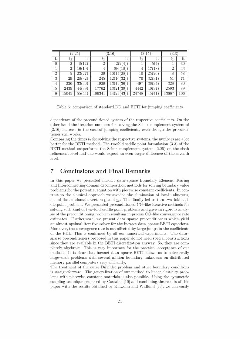
(2.25) (3.16) (3.15) (3.3)L t2 it t2 it t2 it t2 it0 2 8(12) 2 2(2(4)) 1 5(4) 1 301 2 16(19) 4 6(6(18)) 4 17(18) 2 432 5 23(27) 29 10(14(28)) 10 25(26) 8 583 29 28(32) 245 12(16(32)) 70 32(31) 51 714 226 33(36) 1929 13(19(36)) 497 36(34) 328 805 2439 44(39) 17762 13(21(39)) 4442 40(37) 2593 896 15045 55(44) 106341 14(23(43)) 24748 45(41) 13667 106

Table 6: comparison of standard DD and BETI for jumping coefficients

dependence of the preconditioned system of the respective coefficients. On theother hand the iteration numbers for solving the Schur complement system of(2.16) increase in the case of jumping coefficients, even though the precondi-tioner still works.Comparing the times t2 for solving the respective systems, the numbers are a lotbetter for the BETI method. The twofold saddle point formulation (3.3) of theBETI method outperforms the Schur complement system (2.25) on the sixthrefinement level and one would expect an even larger difference of the seventhlevel.

7 Conclusions and Final Remarks

In this paper we presented inexact data–sparse Boundary Element Tearingand Interconnecting domain decomposition methods for solving boundary valueproblems for the potential equation with piecewise constant coefficients. In con-trast to the classical approach we avoided the elimination of local unknowns,i.e. of the subdomain vectors ti and ui. This finally led us to a two–fold sad-dle point problem. We presented preconditioned CG–like iterative methods forsolving such kind of two–fold saddle point problems and gave an rigorous analy-sis of the preconditioning problem resulting in precise CG–like convergence rateestimates. Furthermore, we present data–sparse preconditioners which yieldan almost optimal iterative solver for the inexact data–sparse BETI equations.Moreover, the convergence rate is not affected by large jumps in the coefficientsof the PDE. This is confirmed by all our numerical experiments. The data–sparse preconditioners proposed in this paper do not need special constructionssince they are available in the BETI discretization anyway. So, they are com-pletely algebraic. This is very important for the practical acceptance of ourmethod. It is clear that inexact data–sparse BETI allows us to solve reallylarge–scale problems with several million boundary unknowns on distributedmemory parallel computers very efficiently.The treatment of the outer Dirichlet problem and other boundary conditionsis straightforward. The generalization of our method to linear elasticity prob-lems with piecewise constant materials is also possible. Using the symmetriccoupling technique proposed by Costabel [10] and combining the results of thispaper with the results obtained by Klawonn and Widlund [33], we can easily

24

construct and analyze inexact FETI–BETI solvers for large scale coupled fi-nite and boundary element equations. Exact FETI–BETI solvers were alreadyproposed and analyzed in [39].

References

[1] M. Bebendorf: Approximation of boundary element matrices. Nu-mer. Math. 86 (2000) 565–589.

[2] M. Bebendorf: Effiziente numerische Losung von Randintegralgleichungenunter Verwendung von Niedrigrang–Matrizen. Doctoral Thesis, Universitatdes Saarlandes, 2000.

[3] M. Bebendorf, S. Rjasanow: Adaptive low–rank approximation of colloca-tion matrices. Computing 70 (2003) 1–24.

[4] C. Borgers: The Neumann–Dirichlet domain decomposition method withinexact solvers on the subdomains. Numer. Math. 55 (1989) 123–136.

[5] J. H. Bramble, J. E. Pasciak: A preconditioning technique for indef-inite systems resulting from mixed approximations of elliptic problems.Math. Comp. 50 (1988) 1–17.

[6] J. H. Bramble, J. E. Pasciak, J. Xu: Parallel multilevel preconditioners.Math. Comp. 55 (1990) 1–22.

[7] S. C. Brenner: An additive Schwarz preconditioner for the FETI method.Numer. Math. 94 (2003) 1–31.

[8] J. Carrier, L. Greengard, V. Rokhlin: A fast adaptive multipole algorithmfor particle simulations. SIAM J. Sci. Stat. Comput. 9 (1988) 669–686.

[9] C. Carstensen, M. Kuhn, U. Langer: Fast parallel solvers for symmet-ric boundary element domain decomposition equations. Numer. Math. 79(1998) 321–347.

[10] M. Costabel: Symmetric methods for the coupling of finite elements andboundary elements. In: Boundary Elements IX (C. A. Brebbia, G. Kuhn,W. L. Wendland eds.), Springer, Berlin, pp. 411–420, 1987.

[11] M. Costabel: Boundary integral operators on Lipschitz domains: Elemen-tary results. SIAM J. Math. Anal. 19 (1988) 613–626.

[12] W. Dahmen, S. Prossdorf, R. Schneider: Wavelet approximation methodsfor pseudodifferential equations II: Matrix compression and fast solution.Adv. Comput. Math. 1 (1993) 259–335.

[13] C. Farhat, M. Lesoinne, A. P. Macedo: A two–level domain decomposi-tion method for the iterative solution of high frequency exterior Helmholtzproblems. Numer. Math. 85 (2000) 283–308.

[14] C. Farhat, M. Lesoinne, P. Le Tallec, K. Pierson, D. Rixen: FETI–DP: Adual–primal unified FETI method I: A faster alternative to the two–levelFETI method. Int. J. Numer. Meth. Engrg. 50 (2001) 1523–1544.

25

[15] C. Farhat, M. Lesoinne, K. Pierson: A scalable dual–primal domain de-composition method. Numer. Linear Algebra Appl. 7 (2000) 687–714.

[16] C. Farhat, F.–X. Roux: A method of finite element tearing and intercon-necting and its parallel solution algorithm. Int. J. Numer. Meth. Engrg. 32(1991) 1205–1227.

[17] C. Farhat, F.–X. Roux: Implicit parallel processing in structural mechanics.Comput. Mech. Adv. 2 (1994) 1–124.

[18] Y. Fragakis, M. Papadrakakis: A unified framework for formulating do-main decomposition methods in structural mechanics. Technical Report,National Technical University, Athen, 2002.

[19] S. A. Funken, E. P. Stephan: The BPX preconditioner for the single layerpotential operator. Appl. Anal. 67 (1997) 327–340.

[20] G. N. Gatica, N. Heuer: Conjugate gradient method for dual–dual mixedformulations. Math. Comp. 71 (2002) 1455–1472.

[21] L. Greengard: The Rapid Evaluation of Potential Fields in Particle Simu-lation. The MIT Press, Cambridge, MA, 1987.

[22] L. Greengard, V. Rokhlin: A fast algorithm for particle simulations.J. Comput. Phys. 73 (1987) 325–348.

[23] G. Haase, B. Heise, M. Kuhn, U. Langer: Adaptive domain decompositionmethods for finite and boundary element equations. In: Boundary ElementTopics (W. L. Wendland ed.), Springer, Berlin, pp. 121–147, 1998.

[24] G. Haase, U. Langer, A. Meyer: The approximate Dirichlet domain decom-position method. Computing 47 (1991) 137–167.

[25] G. Haase, U. Langer, A. Meyer, S. Nepomnyaschikh: Hierarchical extensionoperators and local multigrid methods in domain decomposition precondi-tioners. East–West J. Numer. Math. 2 (1994) 173–193.

[26] G. Haase, S. Nepomnyaschikh: Explicit extension operators on hierarchicalgrids. East–West J. Numer. Math. 5 (1997) 231–248.

[27] W. Hackbusch: A sparse matrix arithmetic based on H–matrices. Comput-ing 62 (1999) 89–108.

[28] W. Hackbusch, Z. P. Nowak: On the fast matrix multiplication in theboundary element method by panel clustering. Numer. Math. 54 (1989)463–491.

[29] E. W. Hobson: The Theory of Spherical and Ellipsoidal Harmonics.Chelsea, New York, 1955.

[30] G. C. Hsiao, O. Steinbach, W. L. Wendland: Domain decomposition meth-ods via boundary integral equations. J. Comput. Appl. Math. 125 (2000)521–537.

26

[31] G. C. Hsiao, W. L. Wendland: Domain decomposition in boundary ele-ment methods. In: Proceedings of the Fourth International Symposiumon Domain Decomposition Methods for Partial Differential Equations(R. Glowinski, Y. A. Kuznetsov, G. Meurant, J. Periaux, O. B. Widlundeds.), SIAM, Philadelphia, pp. 41–49, 1991.

[32] M. Kaltenbacher: Numerical Simulation of Mechatronic Sensors and Actu-ators. Springer, Heidelberg, 2004.

[33] A. Klawonn, O. B. Widlund: A domain decomposition method withLagrange multipliers and inexact solvers for linear elasticity. SIAMJ. Sci. Comput. 22 (2000) 1199–1219.

[34] A. Klawonn, O. B. Widlund: FETI and Neumann–Neumanniterative substructuring methods: Connections and new results.Comm. Pure Appl. Math. 54 (2001) 57–90.

[35] A. Klawonn, O. B. Widlund, M. Dryja: Dual–primal FETI methodsfor three–dimensional elliptic problems with heterogeneous coefficients.SIAM J. Numer. Anal. 40 (2002) 159–179.

[36] U. Langer: Parallel iterative solution of symmetric coupled FE/BE–equations via domain decomposition. Contemp. Math. 157 (1994) 335–344.

[37] U. Langer, D. Pusch, S. Reitzinger: Efficient preconditioners for boundaryelement matrices based on grey–box algebraic multigrid methods. Int. J.Numer. Methods Engrg. 58 (2003) 1937–1953.

[38] U. Langer, O. Steinbach: Boundary element tearing and interconnectingmethods. Computing 71 (2003) 205–228.

[39] U. Langer, O. Steinbach: Coupled boundary and finite element tearing andinterconnecting methods. In: Proceedings of the 15th International Con-ference on Domain Decomposition (R. Kornhuber, R. Hoppe, J. Periaux,O. Pironneau, O. Widlund, J. Xu eds.), Lecture Notes in ComputationalSciences and Engineering, vol. 40, Springer, Heidelberg, pp. 83–97, 2004.

[40] J. Mandel, R. Tezaur: Convergence of a substructuring method with La-grange multipliers. Numer. Math. 73 (1996) 473–487.

[41] J. Mandel, R. Tezaur: On the convergence of a dual–primal substructuringmethod. Numer. Math. 88 (2001) 543–558.

[42] W. McLean: Strongly Elliptic Systems and Boundary Integral Equations.Cambridge University Press, 2000.

[43] W. McLean, O. Steinbach: Boundary element preconditioners for a hyper-singular integral equation on an interval. Adv. Comput. Math. 11 (1999)271–286.

[44] J. Nedelec: Integral equations with non integrable kernels. Int. Eq. Op-erat. Th. 5 (1982) 562–572.

27

[45] G. Of, O. Steinbach, A fast multipole boundary element method for a mod-ified hypersingular boundary integral equation. In: Proceedings of the In-ternational Conference on Multifield Problems (M. Efendiev, W. L. Wend-land eds.). Springer Lecture Notes in Applied Mechanics, vol. 12, Springer,Berlin, 2003, 163–169.

[46] G. Of, O. Steinbach, W. L. Wendland: The fast multipole method forthe symmetric boundary integral formulation. Bericht 2004/08, SFB 404,Universitat Stuttgart, 2004.

[47] P. Oswald: Multilevel norms in H−1/2(Γ). Computing 61 (1998) 235–255.

[48] J. M. Perez–Jorda, W. Yang: A concise redefinition of the solid sphericalharmonics and its use in the fast multipole method. J. Chem. Phys. 104(1996) 8003–8006.

[49] T. v. Petersdorff, E. P. Stephan: Multigrid solvers and preconditionersfor first kind integral equations. Num. Methods Part. Diff. Eq. 8 (1992)443–450.

[50] K. H. Pierson, P. Raghaven, G. M. Reese: Experiences with FETI–DP ina production level finite element application. In: Proceedings of the 14thInternational Conference on Domain Decomposition Methods (I. Herrera,D. E. Keyes, O. Widlund, R. Yates eds.), DDM.org, pp. 233–240, 2003.

[51] V. Rokhlin: Rapid solution of integral equations of classical potential the-ory . J. Comput. Phys. 60 (1985) 187–207.

[52] D. Stefanica: A numerical study of FETI algorithms for mortar finite ele-ment methods. SIAM J. Sci. Comput. 23 (2001) 1135–1160.

[53] O. Steinbach: Artificial multilevel boundary element preconditioners. Proc.Appl. Math. Mech. 3 (2003) 539–542.

[54] O. Steinbach: Stability estimates for hybrid coupled domain decompositionmethods. Lecture Notes on Mathematics, vol. 1809, Springer, Heidelberg,2003.

[55] O. Steinbach: Numerische Naherungsverfahren fur elliptische Randwert-probleme. Finite Elemente und Randelemente. B. G. Teubner, Stuttgart,Leipzig, Wiesbaden, 2003.

[56] O. Steinbach, W. L. Wendland: The construction of some efficient precon-ditioners in the boundary element method. Adv. Comput. Math. 9 (1998)191–216.

[57] E. P. Stephan: Multilevel methods for the h–, p–, and hp–versions of theboundary element method. J. Comput. Appl. Math. 125 (2000) 503–519.

[58] A. Toselli, O. Widlund: Domain Decomposition Methods – Algorithms andTheory. Springer Series in Computational Mathematics, vol. 34, Springer,New York, 2004.

[59] C. A. White, M. Head–Gordon: Derivation and efficient implementation ofthe fast multipole method. J. Chem. Phys. 101 (1994) 6593–6605.

28

[60] K. Yosida: Applications of fast multipole method to boundary integralequation method. Dept. of Global Environment Eng., Kyoto Univ., Japan,2001.

[61] W. Zulehner: Analysis of iterative methods for saddle point problems: Aunified approach. Math. Comp. 71 (2002) 479–505.

[62] W. Zulehner: Uzawa–type methods for block–structured indefinite lin-ear systems. SFB–Report 2005-05, SFB F013, Johannes Kepler UniversityLinz, Austria, 2005.

29