SOURCES OF EMITTANCE GROWTH - cds.cern.ch · SOURCES OF EMITTANCE GROWTH D. Möhl CERN, Geneva, ... For hadrons, i.e., proton and ion beams, the geometri cal emittance is appropriate

SOURCES OF EMITTANCE GROWTH

D. Möhl CERN, Geneva, Switzerland

Abstract This note discusses a variety of mechanisms that can lead to a blow-up of the normalized emittance of a particle beam: mismatch at transfer from one machine to the next; scattering on a foil or an internal target, interaction with the residual gas; crossing of resonances; power supply ripple; collective instabilities; intra-beam scattering.

1 INTRODUCTION The notion of beam emittance has been introduced in previous lectures at this school. From these you know that ideally the normalized emittance *ε ε ,βγ= i.e., the emittance multiplied by the relativistic factors β and

εγ is invariant during acceleration. Reality is different! Take the example of

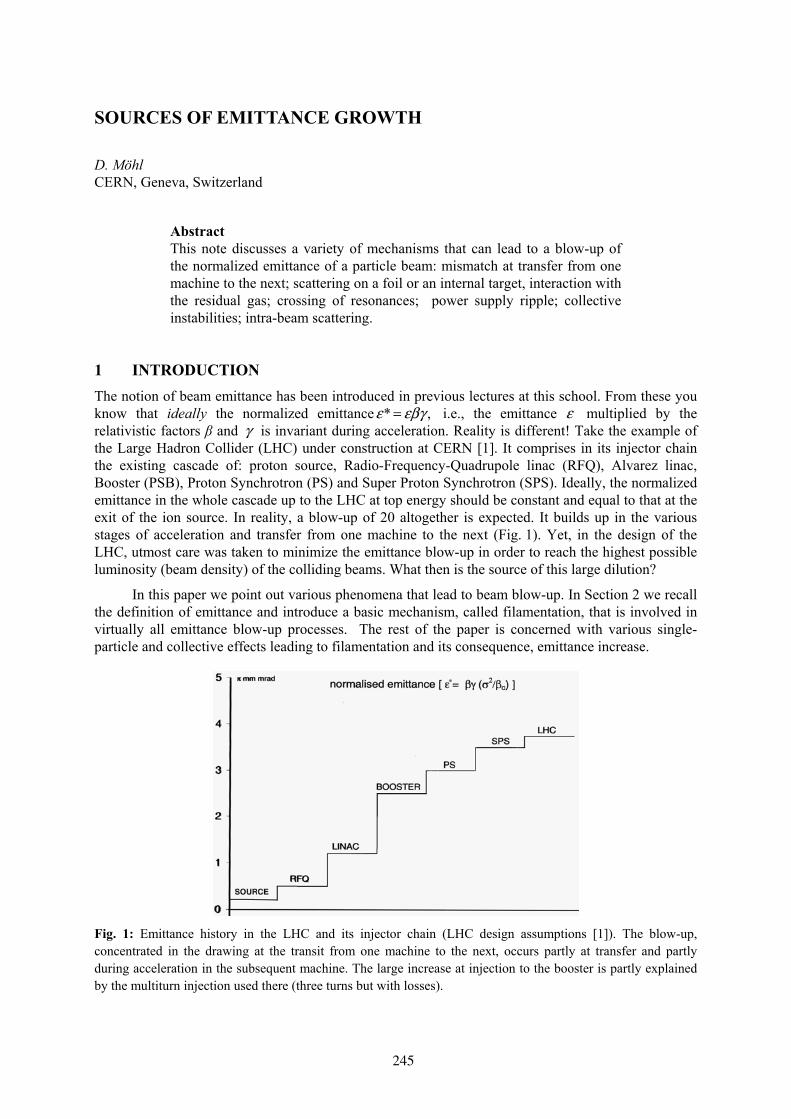
the Large Hadron Collider (LHC) under construction at CERN [1]. It comprises in its injector chain the existing cascade of: proton source, Radio-Frequency-Quadrupole linac (RFQ), Alvarez linac, Booster (PSB), Proton Synchrotron (PS) and Super Proton Synchrotron (SPS). Ideally, the normalized emittance in the whole cascade up to the LHC at top energy should be constant and equal to that at the exit of the ion source. In reality, a blow-up of 20 altogether is expected. It builds up in the various stages of acceleration and transfer from one machine to the next (Fig. 1). Yet, in the design of the LHC, utmost care was taken to minimize the emittance blow-up in order to reach the highest possible luminosity (beam density) of the colliding beams. What then is the source of this large dilution?

In this paper we point out various phenomena that lead to beam blow-up. In Section 2 we recall the definition of emittance and introduce a basic mechanism, called filamentation, that is involved in virtually all emittance blow-up processes. The rest of the paper is concerned with various single-particle and collective effects leading to filamentation and its consequence, emittance increase.

Fig. 1: Emittance history in the LHC and its injector chain (LHC design assumptions [1]). The blow-up, concentrated in the drawing at the transit from one machine to the next, occurs partly at transfer and partly during acceleration in the subsequent machine. The large increase at injection to the booster is partly explained by the multiturn injection used there (three turns but with losses).

245

2 EMITTANCE DEFINITION

2.1 Betatron equation

For convenience we recall here the equation of linear betatron motion [2]–[6], which naturally leads to the definition of emittance. The transverse deviation x(s) of a particle from the design orbit in a beam line or a storage or accelerator ring is governed by the betatron equation

=( ) ( ) ( ) 0x s K s x s′′ + (1)

Here s is the distance along the design orbit, the dash ( / ) denotes derivation with respect to s. It is assumed that the particle moves with constant (or very slowly changing) velocity ( )s in the s direction. The function K(s), in linear approximation a function of only s, is given by the arrangement of focusing elements.

The solution for particle ‘i’ is conveniently written in ‘quasi sinusoidal’ form as:

cos( )

1 / { cos( ) sin( ) }

i ix

i x ix

x A

x A

β δ

iβ α δ

= Ψ +

′ = − Ψ + + Ψ + δ (2)

or equivalently

cos( )

sin( ) .

i ix

x x x i ix

x A

p x x A

β δ

α β β δ

= Ψ +

′≡ + = − Ψ + (3)

The amplitude function xβ , required to perform the transformation from Eq. (1) to Eqs. (2) and (3), is related to K(s) by another differential equation (the envelope equation [2]–[6]). Usually ( )x sβ as well as other optical parameters are obtained by lattice programs like MAD [7]. All one has to do is to input the focusing structure K(s) and appropriate boundary conditions. In a circular machine (with

circumference C), the ‘cyclic’ condition ( , )( 0) ( , )( )x x x xs s Cβ β β β= = =′ ′ leads automatically to a

unique solution. In a beam line, usually andx xβ β ′ at the entrance are prescribed in order to match the β function of the preceding stage. With this or any other two-boundary conditions, the β function of a beam line with a given arrangement of focusing elements is also fully determined.

The phase function ( )sΨ and the function ( )x sα follow directly from ( ):x sβ

1,

( ) 2xx

ds ss

α ββ

′Ψ = = −∫1

( ) . (4)

The following function is also frequently used:

( )211 ( )2( ) .( )x

ss

s

βγ

β

′+= (5)

Finally, the constants and in Eqs. (2) and (3) are given by the initial conditions of particle i. iA iδ

All this has been treated in numerous articles, lecture notes, and textbooks on transverse beam dynamics (see, for example Refs. [2]–[5]) since the classical paper of Courant and Snyder [6]. The essentials are repeated here to be self-contained and to introduce the notation.

D. MOHL

246

2.2 Single-particle emittance

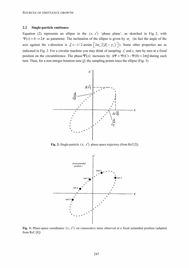
Equation (2) represents an ellipse in the ( , )x x′ ‘phase plane’, as sketched in Fig. 2, with as parameter. The inclination of the ellipse is given by ( ) 0 2s πΨ = → xα (in fact the angle of the

axis against the x-direction is ( )1/ 2 arctan 2 x x xξ α β= − − γ⎡ ⎤⎣ ⎦ ). Some other properties are as

indicated in Fig. 2. For a circular machine you may think of sampling and i ix x′ turn by turn at a fixed position on the circumference. The phase increases by during each turn. Then, for a non-integer betatron tune Q, the sampling points trace the ellipse (Fig. 3).

( )sΨ ( ) (0) 2C πΔΨ = Ψ − Ψ = Q

Fig. 2: Single-particle ( , )x x′ phase-space trajectory (from Ref [2])

Fig. 3: Phase-space coordinates ( , )x x′ on consecutive turns observed at a fixed azimuthal position (adapted from Ref. [8])


247

i

The area of this ellipse, 2Aiπ , is entirely determined by the amplitude A of the motion. This area is closely related to the emittance. We use the convention that the is ‘absorbed into the units’. Thus (with units

i

π2

i Aε = π m rad) is the definition of the ‘single-particle emittance’ or ‘Courant and Snyder invariant’. It can be expressed in various different forms (see Fig. 2) e.g., 2 2

max / ,i i i xA xε γ′= =

or [for any pair ( , )i ix p ], 2 2( ) /i i i xx pε ,β= + or especially

2max /i ixε xβ= . (6)

Please remember that throughout we define the emittance as ‘area’ in phase space with units ‘ radian metre’ [ rad m]! In some publications (e.g. [2]) is defined as emittance. π π 2

iAπ

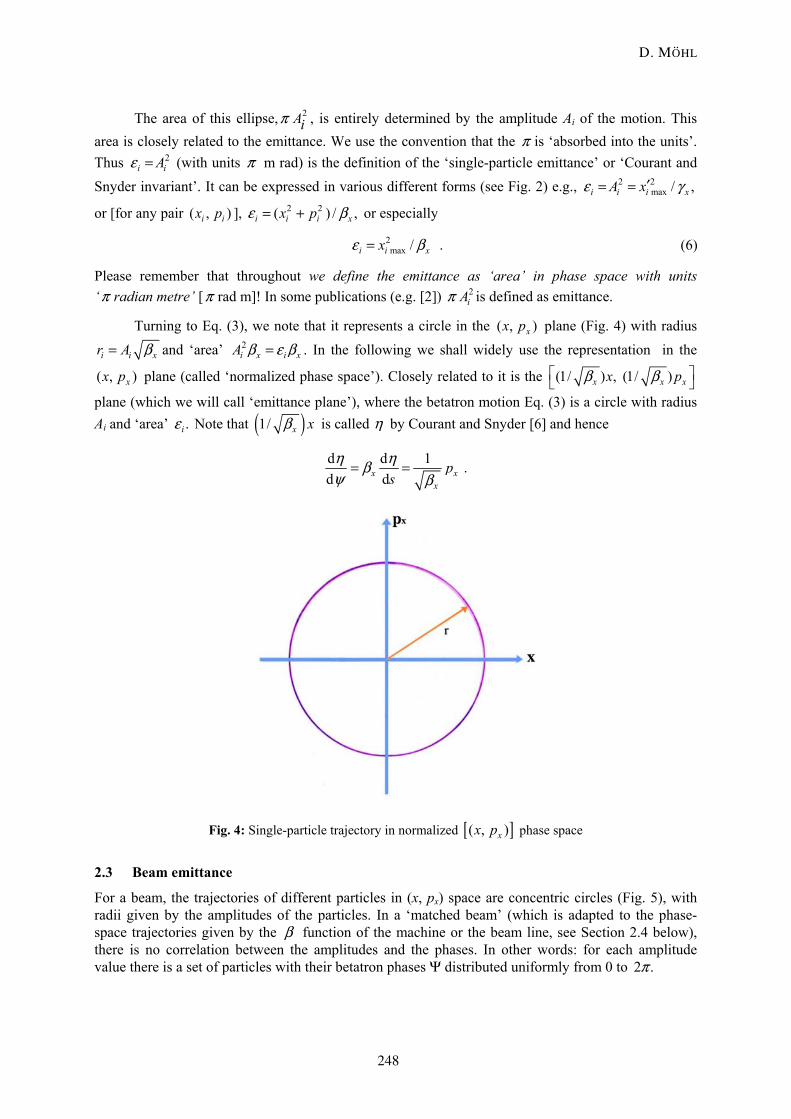
Turning to Eq. (3), we note that it represents a circle in the ( , )xx p plane (Fig. 4) with radius

i ir A xβ= and ‘area’ 2i x i xA β ε β= . In the following we shall widely use the representation in the

( , )xx p plane (called ‘normalized phase space’). Closely related to it is the (1/ ) , (1/ )x x xx pβ β⎡ ⎤⎣ ⎦

plane (which we will call ‘emittance plane’), where the betatron motion Eq. (3) is a circle with radius Ai and ‘area’ Note that .iε (1/ x ) xβ is called η by Courant and Snyder [6] and hence

d d 1 .d dx x

x

ps

η ηβψ β

= =

Fig. 4: Single-particle trajectory in normalized [ ]( , )xx p phase space

2.3 Beam emittance

For a beam, the trajectories of different particles in (x, px) space are concentric circles (Fig. 5), with radii given by the amplitudes of the particles. In a ‘matched beam’ (which is adapted to the phase-space trajectories given by the β function of the machine or the beam line, see Section 2.4 below), there is no correlation between the amplitudes and the phases. In other words: for each amplitude value there is a set of particles with their betatron phases Ψ distributed uniformly from 0 to 2 .π

D. MOHL

248

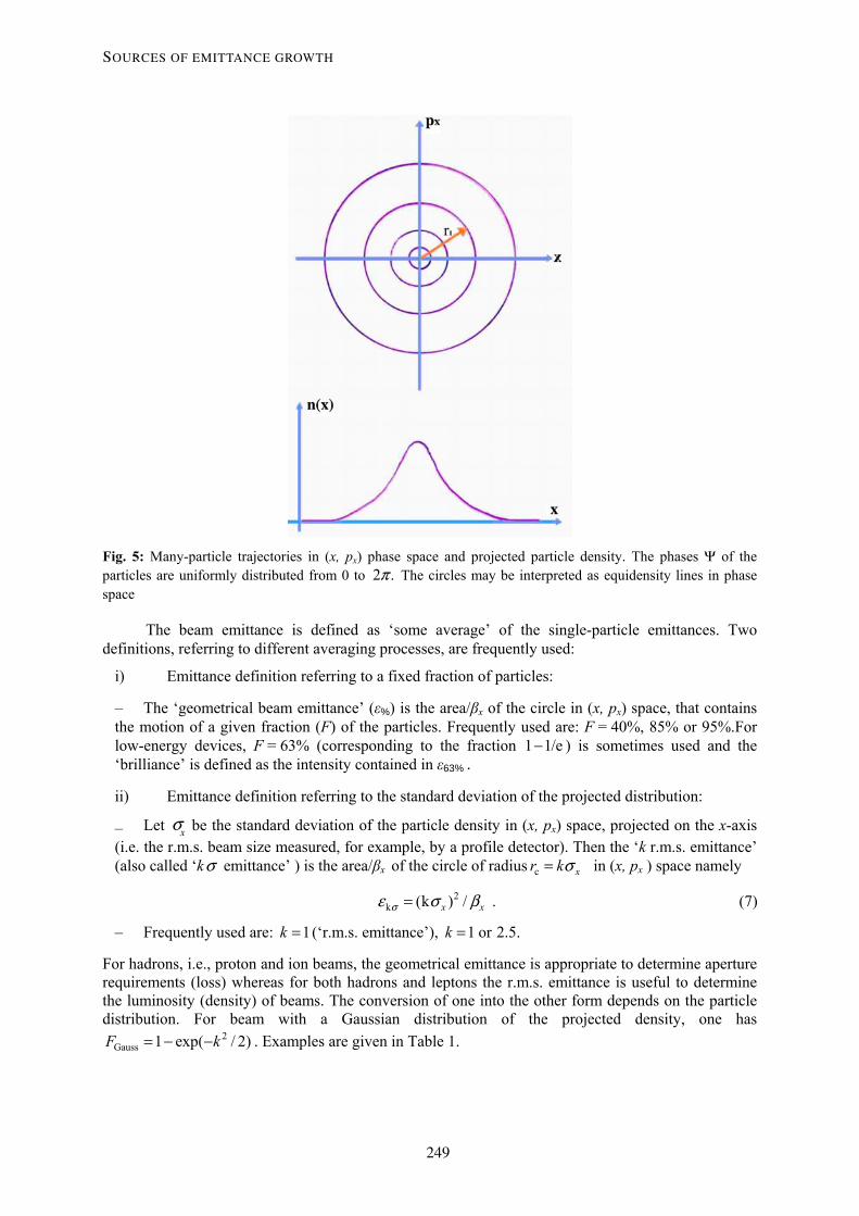
Fig. 5: Many-particle trajectories in (x, px) phase space and projected particle density. The phases Ψ of the particles are uniformly distributed from 0 to The circles may be interpreted as equidensity lines in phase space

2 .π

The beam emittance is defined as ‘some average’ of the single-particle emittances. Two definitions, referring to different averaging processes, are frequently used:

i) Emittance definition referring to a fixed fraction of particles:

– The ‘geometrical beam emittance’ (ε%) is the area/βx of the circle in (x, px) space, that contains the motion of a given fraction (F) of the particles. Frequently used are: F = 40%, 85% or 95%.For low-energy devices, F = 63% (corresponding to the fraction 1 1 ) is sometimes used and the ‘brilliance’ is defined as the intensity contained in ε

/e−63% .

ii) Emittance definition referring to the standard deviation of the projected distribution:

– Let xσ be the standard deviation of the particle density in (x, px) space, projected on the x-axis (i.e. the r.m.s. beam size measured, for example, by a profile detector). Then the ‘k r.m.s. emittance’ (also called ‘k emittance’ ) is the area/βσ x of the circle of radius c xr kσ= in (x, px ) space namely

2k (k ) /x xσε σ β= . (7)

– Frequently used are: (‘r.m.s. emittance’), 1k = 1 or 2.5.k =

For hadrons, i.e., proton and ion beams, the geometrical emittance is appropriate to determine aperture requirements (loss) whereas for both hadrons and leptons the r.m.s. emittance is useful to determine the luminosity (density) of beams. The conversion of one into the other form depends on the particle distribution. For beam with a Gaussian distribution of the projected density, one has

. Examples are given in Table 1. 2Gauss 1 exp( / 2)F = − −k


249

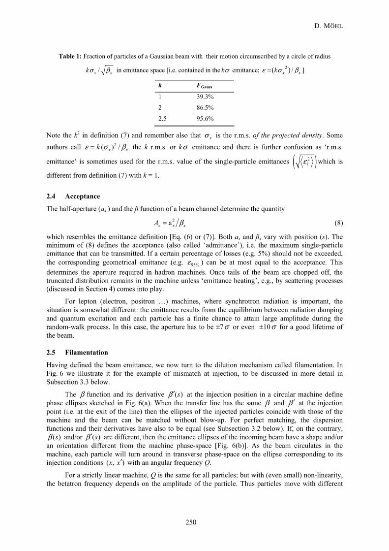
Table 1: Fraction of particles of a Gaussian beam with their motion circumscribed by a circle of radius

/x xkσ β in emittance space [i.e. contained in the emittance; kσ 2 /( )x xkε σ β= ]

k FGauss

1 39.3%

2 86.5%

2.5 95.6%

Note the k2 in definition (7) and remember also that xσ is the r.m.s. of the projected density. Some authors call 2( ) /x xkε σ β= the k r.m.s. or k emittance and there is further confusion as ‘r.m.s.

emittance’ is sometimes used for the r.m.s. value of the single-particle emittances

σ

( 2iε ) which is

different from definition (7) with k = 1.

2.4 Acceptance

The half-aperture (ax ) and the β function of a beam channel determine the quantity 2ax x xA β= (8)

which resembles the emittance definition [Eq. (6) or (7)]. Both ax and βx vary with position (s). The minimum of (8) defines the acceptance (also called ‘admittance’), i.e. the maximum single-particle emittance that can be transmitted. If a certain percentage of losses (e.g. 5%) should not be exceeded, the corresponding geometrical emittance (e.g. ) can be at most equal to the acceptance. This determines the aperture required in hadron machines. Once tails of the beam are chopped off, the truncated distribution remains in the machine unless ‘emittance heating’, e.g., by scattering processes (discussed in Section 4) comes into play.

95%ε

For lepton (electron, positron …) machines, where synchrotron radiation is important, the situation is somewhat different: the emittance results from the equilibrium between radiation damping and quantum excitation and each particle has a finite chance to attain large amplitude during the random-walk process. In this case, the aperture has to be ±7 or even ±10 for a good lifetime of the beam.

σ σ

2.5 Filamentation

Having defined the beam emittance, we now turn to the dilution mechanism called filamentation. In Fig. 6 we illustrate it for the example of mismatch at injection, to be discussed in more detail in Subsection 3.3 below.

The β function and its derivative ( )sβ ′ at the injection position in a circular machine define phase ellipses sketched in Fig. 6(a). When the transfer line has the same β and β ′ at the injection point (i.e. at the exit of the line) then the ellipses of the injected particles coincide with those of the machine and the beam can be matched without blow-up. For perfect matching, the dispersion functions and their derivatives have also to be equal (see Subsection 3.2 below). If, on the contrary,

( )sβ and/or ( )sβ ′ are different, then the emittance ellipses of the incoming beam have a shape and/or an orientation different from the machine phase-space [Fig. 6(b)]. As the beam circulates in the machine, each particle will turn around in transverse phase-space on the ellipse corresponding to its injection conditions ( , )x x′ with an angular frequency Q.

For a strictly linear machine, Q is the same for all particles; but with (even small) non-linearity, the betatron frequency depends on the amplitude of the particle. Thus particles move with different

D. MOHL

250

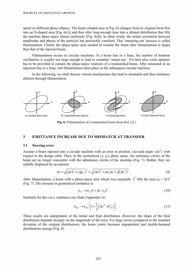
speed on different phase ellipses. The beam (shaded area in Fig. 6) changes from its original form first into an S-shaped area [Fig. 6(c)] and then after long-enough time into a diluted distribution that fills the machine phase-space almost uniformly [Fig. 6(d)]. In other words, the initial correlation between amplitudes and phases of the particles has practically vanished. This ‘smearing-out’ process is called filamentation. Clearly the phase-space area needed to contain the beam after filamentation is larger than that of the injected beam.

Filamentation occurs in circular machines. In a beam line or a linac, the number of betatron oscillations is usually not large enough to lead to complete ‘smear-out’. Yet here also, extra aperture has to be provided to contain the phase-space rotations of a mismatched beam. After mismatch in an injection line or a linac, full filamentation takes place in the subsequent circular machine.

In the following, we shall discuss various mechanisms that lead to mismatch and thus emittance dilution through filamentation.

Fig. 6: Filamentation of a mismatched beam (from Ref. [2] )

3 EMITTANCE INCREASE DUE TO MISMATCH AT TRANSFER

3.1 Steering error

Assume a beam injected into a circular machine with an error in position ( )xΔ and angle ( )x′Δ with respect to the design orbit. Then, in the normalized (x, px) phase space, the emittance circles of the beam are no longer concentric with the admittance circles of the machine (Fig. 7). Rather, they are radially displaced by an amount

2 2 2( ) ( ) ( ) ( )x xr x p x x xα β ′Δ = Δ + Δ = Δ + Δ + Δ 2x . (9)

After filamentation, a beam with a phase-space area which was originally fills the area (r2

0r 0 + Δr)2 (Fig. 7). The increase in geometrical emittance is

2% % 0(1 / )r rε ε→ + Δ . (10)

Similarly for the r.m.s. emittance one finds (Appendix A)

( )2 2,0

11 /2k k xrσ σε ε σ⎧ ⎫→ + Δ⎨ ⎬

⎩ ⎭ . (11)

These results are independent of the initial and final distribution. However, the shape of the final distribution depends strongly on the magnitude of the error. For large errors (compared to the standard deviation of the original distribution), the beam centre becomes depopulated and double-humped distributions emerge (Fig. 8).


251

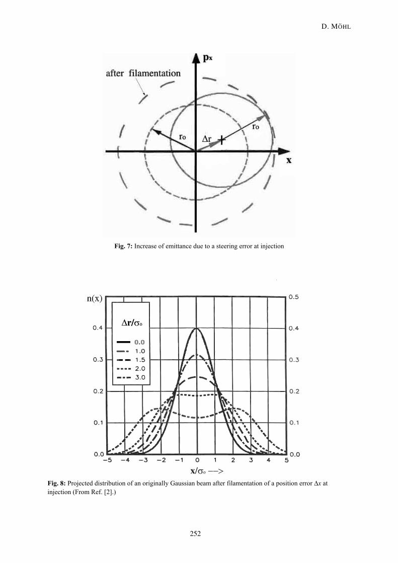
Fig. 7: Increase of emittance due to a steering error at injection

Fig. 8: Projected distribution of an originally Gaussian beam after filamentation of a position error Δx at injection (From Ref. [2].)

D. MOHL

252

These double humps are a sign of big steering errors at transfer in contrast with a mismatch of the β function (to be discussed in Subsection 3.3), which leads mainly to a widening of the distribution.

3.2 Momentum error and dispersion-function mismatch

Assume that a beam with a momentum p pδ+ is injected into a machine adjusted for the momentum p on its central orbit. If the dispersion D of the line and the machine are matched (D and are the same) and the beam is injected onto the off-momentum orbit with

D′/x D p pδ δ= and / ,x D p pδ δ′ ′=

then perfect matching can be achieved. If, however, injection is made directly onto the central orbit, then this is equivalent to a steering error Δx = Dδp/p, /x D p pδ′ ′Δ = and our previous results [Eqs. (10) and (11)] can be used putting

( ){ }1/ 222 /x xr D D D p pβ α δ′Δ = + + . (12)

Next, imagine that the dispersion functions of the line and the machine at the injection location differ. We can assume without loss of generality that the machine has D = 0 and at the injection point (in the general case replace

0D′ =; D D D D′→ Δ → Δ ′ in the following). For each momentum p + Δp

we have an equivalent steering error Δx = DΔp/p and /x D p p′ ′Δ = Δ . Thus the momentum distribution is folded into the transverse phase-space. The blow-up in geometrical emittance after filamentation depends on both the transverse and the momentum distribution. An approximation is to calculate the blow-up from Eq. (11) putting

( ){ } ( )1/ 222

%/x xr D D D p pβ α′Δ = + + Δ . (13)

Here ±(Δp/p)% is momentum spread containing the prescribed fraction of the momentum distribution.

For the increase of the r.m.s. emittance one obtains (Appendix B)

( ){ }( )222 2p 0

112k k x xD D D pσ σε ε / /β α σ σ⎧ ⎫′→ + + +⎨ ⎬

⎩ ⎭ . (14)

This result is independent of the shape of the momentum distribution and also independent of the initial and final transverse distribution. Equation (14) indicates that in the case of dispersion mismatch the momentum distribution is folded into the transverse emittance.

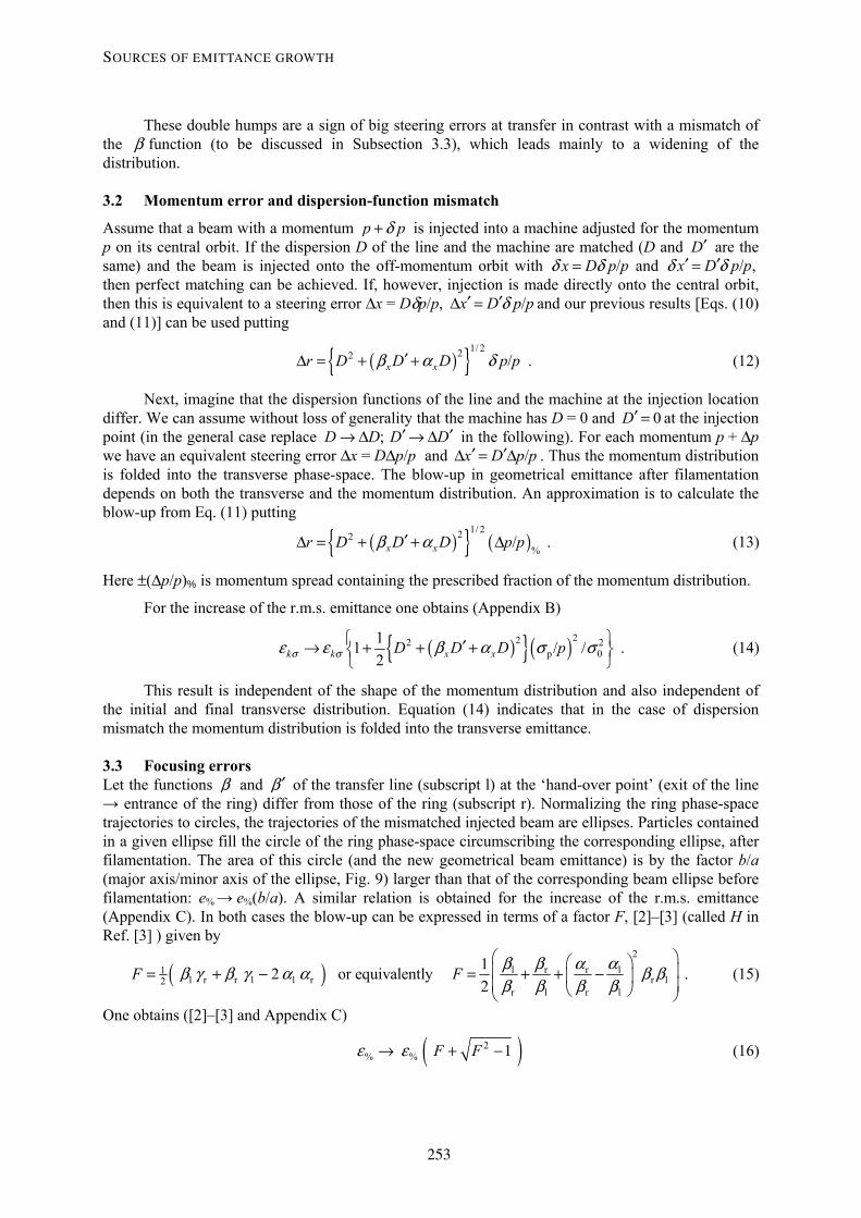
3.3 Focusing errors Let the functions β and β ′ of the transfer line (subscript l) at the ‘hand-over point’ (exit of the line → entrance of the ring) differ from those of the ring (subscript r). Normalizing the ring phase-space trajectories to circles, the trajectories of the mismatched injected beam are ellipses. Particles contained in a given ellipse fill the circle of the ring phase-space circumscribing the corresponding ellipse, after filamentation. The area of this circle (and the new geometrical beam emittance) is by the factor b/a (major axis/minor axis of the ellipse, Fig. 9) larger than that of the corresponding beam ellipse before filamentation: e → e (b/a). A similar relation is obtained for the increase of the r.m.s. emittance (Appendix C). In both cases the blow-up can be expressed in terms of a factor F, [2]–[3] (called H in Ref. [3] ) given by

% %

( )2

l r r l1l r r l l r r l2

r l r l

12 or equivalently 2

F F β β α αβ γ β γ α α β ββ β β β

⎛ ⎞⎛ ⎞⎜ ⎟= + − = + + −⎜ ⎟⎜ ⎟⎝ ⎠⎝ ⎠ . (15)

One obtains ([2]–[3] and Appendix C)

( )2% % 1F Fε ε→ + − (16)


253

k k Fσ σε ε→ . (17)

Fig. 9: Mismatch due to focusing errors

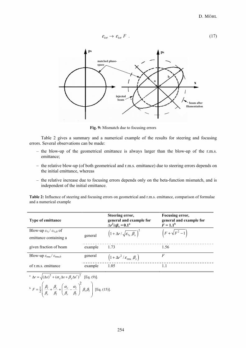
Table 2 gives a summary and a numerical example of the results for steering and focusing errors. Several observations can be made:

– the blow-up of the geometrical emittance is always larger than the blow-up of the r.m.s. emittance;

– the relative blow-up (of both geometrical and r.m.s. emittance) due to steering errors depends on the initial emittance, whereas

– the relative increase due to focusing errors depends only on the beta-function mismatch, and is independent of the initial emittance.

Table 2: Influence of steering and focusing errors on geometrical and r.m.s. emittance, comparison of formulae and a numerical example

Type of emittance

Steering error, general and example for ∆r2/εβx = 0.1a

Focusing error, general and example for F = 1.1b

Blow-up ε% / ε%,0 of

emittance containing a

general ( )2

%1 / xr ε β+ Δ ( )2 1F F+ −

given fraction of beam example 1.73 1.56 Blow-up εrms / εrms,0 general ( )2

rms1 / xr ε β+ Δ F

of r.m.s. emittance example 1.05 1.1

2 2( ) ( )x xr x x xα β ′Δ = Δ + Δ + Δa [Eq. (9)].

b

212

l lr rr l

r l r lF

β αβ αβ β

β β β β= + + −

⎛ ⎞⎛ ⎞⎜ ⎟⎜ ⎟⎜ ⎟⎝ ⎠⎝ ⎠ [Eq. (15)].

D. MOHL

254

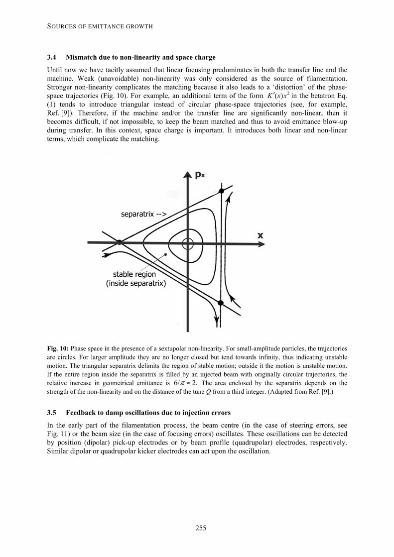
3.4 Mismatch due to non-linearity and space charge

Until now we have tacitly assumed that linear focusing predominates in both the transfer line and the machine. Weak (unavoidable) non-linearity was only considered as the source of filamentation. Stronger non-linearity complicates the matching because it also leads to a ‘distortion’ of the phase-space trajectories (Fig. 10). For example, an additional term of the form in the betatron Eq. (1) tends to introduce triangular instead of circular phase-space trajectories (see, for example, Ref. [9]). Therefore, if the machine and/or the transfer line are significantly non-linear, then it becomes difficult, if not impossible, to keep the beam matched and thus to avoid emittance blow-up during transfer. In this context, space charge is important. It introduces both linear and non-linear terms, which complicate the matching.

2( )K s x′

Fig. 10: Phase space in the presence of a sextupolar non-linearity. For small-amplitude particles, the trajectories are circles. For larger amplitude they are no longer closed but tend towards infinity, thus indicating unstable motion. The triangular separatrix delimits the region of stable motion; outside it the motion is unstable motion. If the entire region inside the separatrix is filled by an injected beam with originally circular trajectories, the relative increase in geometrical emittance is The area enclosed by the separatrix depends on the strength of the non-linearity and on the distance of the tune Q from a third integer. (Adapted from Ref. [9].)

6/ 2.π ≈

3.5 Feedback to damp oscillations due to injection errors

In the early part of the filamentation process, the beam centre (in the case of steering errors, see Fig. 11) or the beam size (in the case of focusing errors) oscillates. These oscillations can be detected by position (dipolar) pick-up electrodes or by beam profile (quadrupolar) electrodes, respectively. Similar dipolar or quadrupolar kicker electrodes can act upon the oscillation.


255

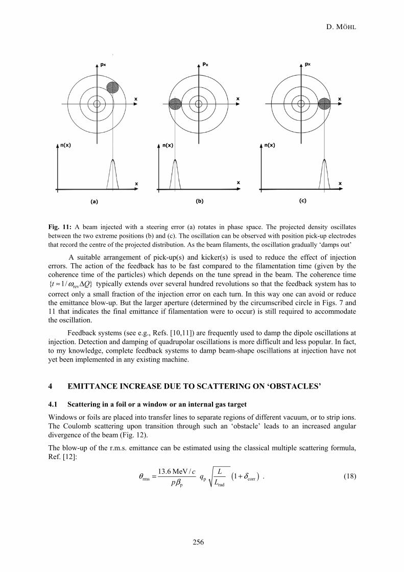
Fig. 11: A beam injected with a steering error (a) rotates in phase space. The projected density oscillates between the two extreme positions (b) and (c). The oscillation can be observed with position pick-up electrodes that record the centre of the projected distribution. As the beam filaments, the oscillation gradually ‘damps out’

A suitable arrangement of pick-up(s) and kicker(s) is used to reduce the effect of injection errors. The action of the feedback has to be fast compared to the filamentation time (given by the coherence time of the particles) which depends on the tune spread in the beam. The coherence time

typically extends over several hundred revolutions so that the feedback system has to correct only a small fraction of the injection error on each turn. In this way one can avoid or reduce the emittance blow-up. But the larger aperture (determined by the circumscribed circle in Figs. 7 and 11 that indicates the final emittance if filamentation were to occur) is still required to accommodate the oscillation.

rev{ 1/ }t ω≈ ΔQ

Feedback systems (see e.g., Refs. [10,11]) are frequently used to damp the dipole oscillations at injection. Detection and damping of quadrupolar oscillations is more difficult and less popular. In fact, to my knowledge, complete feedback systems to damp beam-shape oscillations at injection have not yet been implemented in any existing machine.

4 EMITTANCE INCREASE DUE TO SCATTERING ON ‘OBSTACLES’

4.1 Scattering in a foil or a window or an internal gas target

Windows or foils are placed into transfer lines to separate regions of different vacuum, or to strip ions. The Coulomb scattering upon transition through such an ‘obstacle’ leads to an increased angular divergence of the beam (Fig. 12).

The blow-up of the r.m.s. emittance can be estimated using the classical multiple scattering formula, Ref. [12]:

( )rms p corrp rad

13.6 MeV / 1c Lqp L

θβ

= + δ . (18)

D. MOHL

256

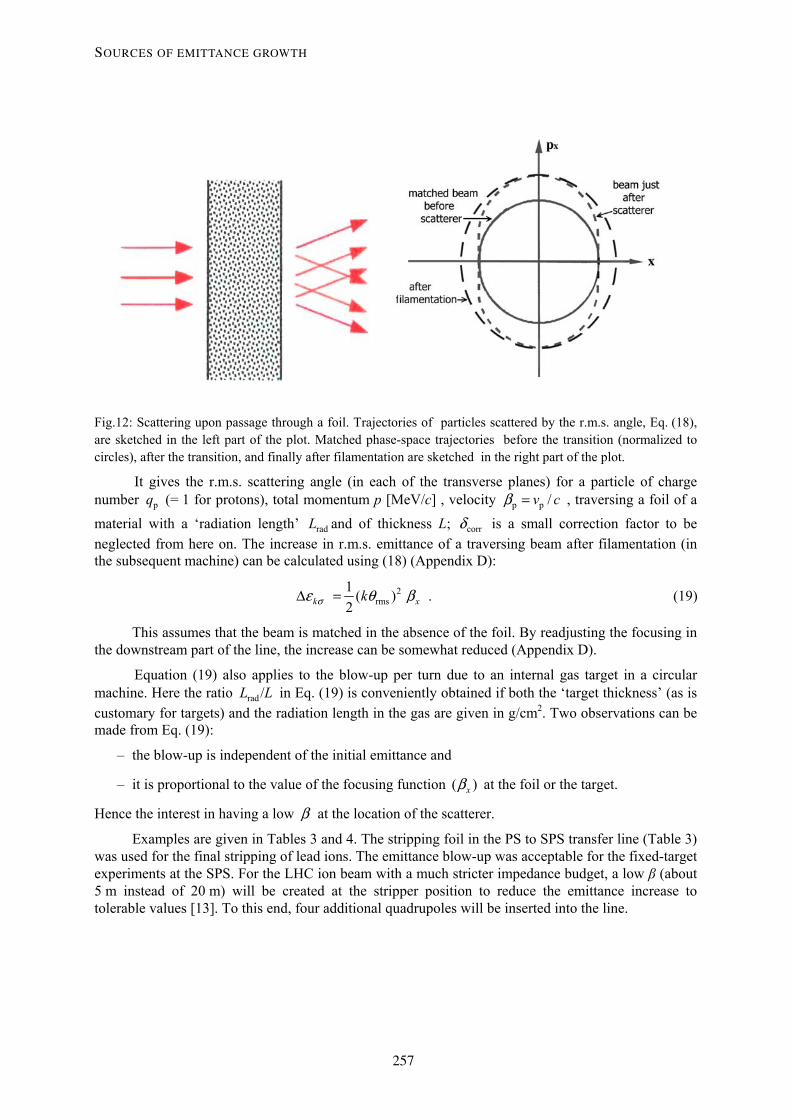
Fig.12: Scattering upon passage through a foil. Trajectories of particles scattered by the r.m.s. angle, Eq. (18), are sketched in the left part of the plot. Matched phase-space trajectories before the transition (normalized to circles), after the transition, and finally after filamentation are sketched in the right part of the plot.

It gives the r.m.s. scattering angle (in each of the transverse planes) for a particle of charge number pq (= 1 for protons), total momentum p [MeV/c] , velocity p p /v cβ = , traversing a foil of a

material with a ‘radiation length’ and of thickness L; is a small correction factor to be neglected from here on. The increase in r.m.s. emittance of a traversing beam after filamentation (in the subsequent machine) can be calculated using (18) (Appendix D):

radL corrδ

2rms

1 ( )2k kσε θ xβΔ = . (19)

This assumes that the beam is matched in the absence of the foil. By readjusting the focusing in the downstream part of the line, the increase can be somewhat reduced (Appendix D).

Equation (19) also applies to the blow-up per turn due to an internal gas target in a circular machine. Here the ratio in Eq. (19) is conveniently obtained if both the ‘target thickness’ (as is customary for targets) and the radiation length in the gas are given in g/cm

rad /L L2. Two observations can be

made from Eq. (19):

– the blow-up is independent of the initial emittance and

– it is proportional to the value of the focusing function ( )xβ at the foil or the target.

Hence the interest in having a low β at the location of the scatterer.

Examples are given in Tables 3 and 4. The stripping foil in the PS to SPS transfer line (Table 3) was used for the final stripping of lead ions. The emittance blow-up was acceptable for the fixed-target experiments at the SPS. For the LHC ion beam with a much stricter impedance budget, a low β (about 5 m instead of 20 m) will be created at the stripper position to reduce the emittance increase to tolerable values [13]. To this end, four additional quadrupoles will be inserted into the line.


257

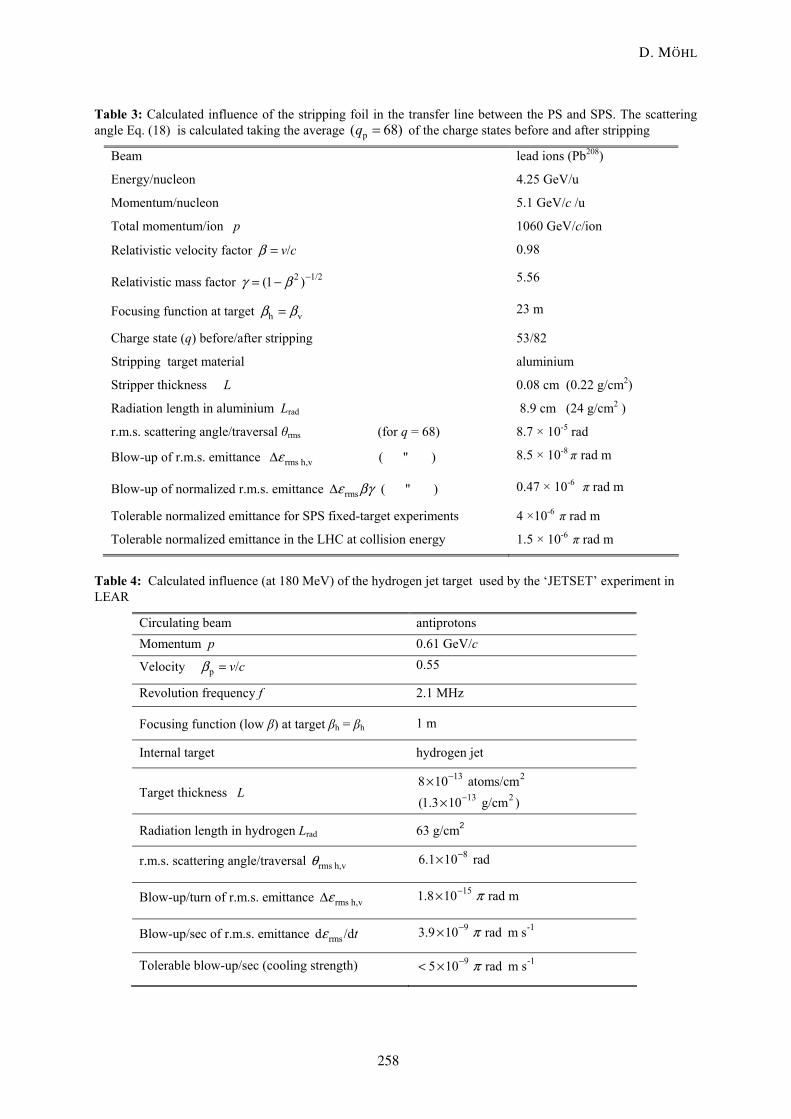
( 68)q =Table 3: Calculated influence of the stripping foil in the transfer line between the PS and SPS. The scattering angle Eq. (18) is calculated taking the average of the charge states before and after stripping p

Beam lead ions (Pb208)

Energy/nucleon 4.25 GeV/u

Momentum/nucleon 5.1 GeV/c /u

Total momentum/ion p 1060 GeV/c/ion

Relativistic velocity factor /v cβ = 0.98

Relativistic mass factor 2 1/2(1 )γ β −= − 5.56

Focusing function at target h vβ β= 23 m

Charge state (q) before/after stripping 53/82

Stripping target material aluminium

Stripper thickness L 0.08 cm (0.22 g/cm2)

Radiation length in aluminium Lrad 8.9 cm (24 g/cm2 )

r.m.s. scattering angle/traversal θrms (for q = 68) 8.7 × 10-5 rad

Blow-up of r.m.s. emittance ( '' ) rms h,vεΔ 8.5 × 10-8 π rad m

Blow-up of normalized r.m.s. emittance rmsε βγΔ ( '' ) 0.47 × 10-6 π rad m

Tolerable normalized emittance for SPS fixed-target experiments 4 ×10-6 π rad m

Tolerable normalized emittance in the LHC at collision energy 1.5 × 10-6 π rad m

Table 4: Calculated influence (at 180 MeV) of the hydrogen jet target used by the ‘JETSET’ experiment in LEAR

Circulating beam antiprotons Momentum p 0.61 GeV/c

Velocity p /v cβ = 0.55

Revolution frequency f 2.1 MHz

Focusing function (low β) at target βh = βh 1 m

Internal target hydrogen jet

Target thickness L 13 28 10 atoms/cm−×

13 2(1.3 10 g/cm )−×

Radiation length in hydrogen Lrad 63 g/cm2

r.m.s. scattering angle/traversal rms h,vθ 86.1 10 rad−×

Blow-up/turn of r.m.s. emittance rms h,vεΔ 151.8 10 rad mπ−×

Blow-up/sec of r.m.s. emittance rmsd /dtε 9 -3.9 10 rad m sπ−× 1

Tolerable blow-up/sec (cooling strength) 9 -5 10 rad m sπ−< × 1

D. MOHL

258

The hydrogen gas jet [14] was used in LEAR up to 1996. A small equilibrium beam size was desirable. It results from the ‘beam heating’ dεrms/dt at the target and ‘beam cooling’ by the stochastic cooling system. For cooling times (for 1010 particles) of the order of 200 s, equilibrium emittances of 1 mm mrad were attainable when the heating was less than 5 × 10π -9 mm mrad sπ -1 (corresponding to a target thickness of less than 1014 atoms/cm2).

4.2 Scattering on the residual gas

t

This subject is treated in many papers of which I find the internal report by W. Hardt [15] especially instructive. Here we can use our previous results by taking the residual gas atmosphere as a ‘distributed thin scatterer’. For pure nitrogen (N2) at pressure P the radiation length is

and the thickness traversed by the beam in time t is 2rad, NL ≈

327 m /( /760 Torr)P p .L cβ= Then from Eqs.

(18) and (19) we get the blow-up of the emittance as kσ

p2 2 2p

p

1 14 MeV /( )2 327 ( / 760 Torr)k x

c tck qp Pσ

βε β

βΔ = .

Here xβ is the average around the ring of the beta function as scattering occurs all around the circumference; p = 931 MeV/c*Ap*βpγp, is the total momentum, where Ap is the mass number of the ion (≈ 1 for protons). Equation (20) leads directly to Hardt’s formula [with a slight difference in the numerical factor as he takes 15 MeV/c in the scattering angle formula (18)]

2p22 3 2p p p

0.14kq P tkAσε xβ

β γΔ ≈ (P [Torr], βx [m], t [sec]) . (20)

Equation (20) is widely used to determine the vacuum requirement in a storage ring. For a synchrotron, one has to integrate 2

p pd /t β γ over the acceleration cycle to obtain the blow-up of the normalized emittance. For a residual atmosphere with different gas components of partial pressures Pi, we can define the N2 equivalent pressure for multiple Coulomb scattering as

( )2 2N equ rad,N rad,i iP P L L=∑ .

The radiation length for some gases at atmospheric pressure is given in Table 5.

Table 5: Radiation length and density (at 760 Torr and 20 °C) for some gases (adapted from Ref. [12])

Gas component H2 He N2 Ne Ar Air unit Density (at 20 °C and 760 Torr) 0.084 0.166 0.116 0.839 1.66 1.20 g/dm3

‘Radiation density’ 63 94.3 38 28.9 19.6 36.1 g/cm2

Radiation length (at 20 °C, 760 Torr) 7500 568 327 344 118 301 m

As an example for vacuum requirements in a storage ring, Table 6 summarizes the situation in LEAR at its lowest energy (5.3 MeV i.e. 100 MeV/c). At this energy, stochastic cooling worked with time constants of say 3 minutes for 10( )τ

rms/dtε 3 -110 mm mrad sπ×

rms/d .tτ εΔ ≈

9 antiprotons when the r.m.s. emittances were 1π mm mrad. Thus a heating rate Δ up to 5 could be tolerated leading to an equilibrium

If smaller equilibrium emittances are desired, a lower vacuum or faster cooling (e.g., electron cooling) is required.

1 mm mradπ


259

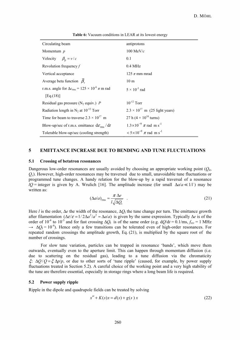
Table 6: Vacuum conditions in LEAR at its lowest energy

Circulating beam antiprotons

Momentum p 100 MeV/c

Velocity p /v cβ = 0.1

Revolution frequency f 0.4 MHz

Vertical acceptance 125 π mm mrad

Average beta function vβ 10 m

r.m.s. angle for Δεrms = 125 × 10-6 π m rad

[Eq.(18)] 5 × 10-3 rad

Residual gas pressure (N2 equiv.) P 10-12 Torr

Radiation length in N2 at 10-12 Torr 2.3 × 1017 m (25 light years)

Time for beam to traverse 2.3 × 1017 m 27 h (4 × 1010 turns)

Blow-up/sec of r.m.s. emittance rmsd / dtε 9 -1.3 10 rad m sπ−× 1

1

Tolerable blow-up/sec (cooling strength) 9 -5 10 rad m sπ−< ×

5 EMITTANCE INCREASE DUE TO BENDING AND TUNE FLUCTUATIONS

5.1 Crossing of betatron resonances

Dangerous low-order resonances are usually avoided by choosing an appropriate working point (Qx, Qy). However, high-order resonances may be traversed due to small, unavoidable tune fluctuations or programmed tune changes. A handy relation for the blow-up by a rapid traversal of a resonance lQ = integer is given by A. Wrulich [16]. The amplitude increase (for small ) may be written as:

/ 1/a a lΔ

rmst

( / ) ea al Qπ ΔΔ ≈

Δ . (21)

Here l is the order, Δe the width of the resonance, ΔQt the tune change per turn. The emittance growth after filamentation is given by the same expression. Typically Δe is of the order of 10

2 2( / 1/ 2 / / )a a a aε εΔ = Δ ≈ Δ-4 to 10-3 and for fast crossing ΔQt is of the same order (e.g. dQ/dt = 0.1/ms, frev = 1 MHz

→ ΔQt = 10-4). Hence only a few transitions can be tolerated even of high-order resonances. For repeated random crossings the amplitude growth, Eq. (21), is multiplied by the square root of the number of crossings.

For slow tune variation, particles can be trapped in resonance ‘bands’, which move them outwards, eventually even to the aperture limit. This can happen through momentum diffusion (i.e. due to scattering on the residual gas), leading to a tune diffusion via the chromaticity

:ξ /Q Q ξΔ = Δp/p, or due to other sorts of ‘tune ripple’ (caused, for example, by power supply fluctuations treated in Section 5.2). A careful choice of the working point and a very high stability of the tune are therefore essential, especially in storage rings where a long beam life is required.

5.2 Power supply ripple

Ripple in the dipole and quadrupole fields can be treated by solving

( ) ( ) ( )x K s x d s g s x′′ + = + (22)

D. MOHL

260

where d(s) and g(s) are small random functions [17] representing bending and focusing ripples. In the context of accelerators, such differential equations are treated in Refs. [18] and [19]. Instead, we can use the previous results, Eqs. (11) and (17), for steering and focusing errors assuming that the particles receive many small random kicks.

We shall consider only dipole errors here, the effect of ripple in the quadrupole supplies can be treated along similar lines. Let be the random deflection error per turn with the variance ( )nθ

2 2rms( )nθ θ= . Each kick introduces an increase in the -emittance of

according to Eq. (11) together with Eqs. (9) and (7). For true (white) noise, the effect of the multiple kicks adds up statistically (i.e. ‘in quadrature’). After n = f

kσ 2kd /d 1/2 [k ( )]n nσε β θ=

rev t turns one therefore has [in analogy with Eq. (20)]:

2k rms

1 ( )2 x k fσε β θΔ = revt . (23)

To get an idea of the orders of magnitude involved, assume that storage for one day is required. For a storage ring like the ISR this means n = frev t ≈ 2.5 × 1010 turns. Take a typical beta function:

20 m,xβ = and assume one magnet giving a nominal angle of mrad with field jitter .Then Eq. (21) yields

mm mrad. This is a sizeable fraction of the acceptance, which is typically 100 π mm mrad. These considerations suggest a necessary field stability

0 10θ =6 2 2 5

rms , rms rms( / ) 10 [10 mrad ( / ) ] (10 mrad)nB B B Bθ−= → = = 2σεΔ =

25 πΔB/B of 1/106. Does this require a similar

current stability (ΔI/I) of the power supply?

In fact, the frequency content of the noise is very important [18,19]. It can be shown that the beam is most sensitive to noise components that coincide in their frequency fk with the ‘betatron sidebands’ of the particles, i.e., if ( ) revmkf Q f= ± (with m = 0, 1, 2, ….). The magnet and its connections act like a filter with a transfer function H(ω). In the simplest case H(ω) = (iωL)-1 is given by the large inductance of the magnet. Then the beam response to ripple in the power supply current is reduced by a filtering factor F

2rev rev 2

rev rev

1H ( ){( ) }m

F m Qm Q L

ω ωω ω

∞ ∞

=−∞ −∞

= + ≈+∑ ∑ . (24)

The lowest sideband (m ≈ –Q) which contributes the dominating effect to the sum has already a frequency of 0.1 × frev to 0.3 × frev , typically in the range of 100 kHz for small and of 1 kHz for very large machines. Then the effective noise, compared to the supply ripple at 50 Hz, is reduced by 3 to 6 orders of magnitude. These qualitative considerations may show the way to evaluate the sensitivity to power supply ripple.

6 INTRA-BEAM SCATTERING Small-angle (multiple) Coulomb scattering between particles of the same beam (‘intra-beam scattering’, Refs. [20]–[25]) is important for dense beams. In the collisions, energy transfer back and forth between all three planes can occur. In a strong-focusing accelerator or storage ring this leads not only to a re-distribution, but unavoidably to a growth of the six-dimensional phase-space volume. In fact in modern storage rings and colliders, intra-beam scattering is one of the dominant effects limiting the luminosity lifetime.


261

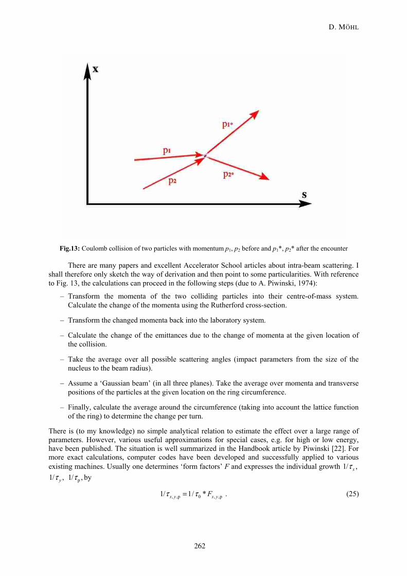
Fig.13: Coulomb collision of two particles with momentum p1, p2 before and p1*, p2* after the encounter

There are many papers and excellent Accelerator School articles about intra-beam scattering. I shall therefore only sketch the way of derivation and then point to some particularities. With reference to Fig. 13, the calculations can proceed in the following steps (due to A. Piwinski, 1974):

– Transform the momenta of the two colliding particles into their centre-of-mass system. Calculate the change of the momenta using the Rutherford cross-section.

– Transform the changed momenta back into the laboratory system.

– Calculate the change of the emittances due to the change of momenta at the given location of the collision.

– Take the average over all possible scattering angles (impact parameters from the size of the nucleus to the beam radius).

– Assume a ‘Gaussian beam’ (in all three planes). Take the average over momenta and transverse positions of the particles at the given location on the ring circumference.

– Finally, calculate the average around the circumference (taking into account the lattice function of the ring) to determine the change per turn.

There is (to my knowledge) no simple analytical relation to estimate the effect over a large range of parameters. However, various useful approximations for special cases, e.g. for high or low energy, have been published. The situation is well summarized in the Handbook article by Piwinski [22]. For more exact calculations, computer codes have been developed and successfully applied to various existing machines. Usually one determines ‘form factors’ F and expresses the individual growth 1/ ,xτ

1/ ,yτ p1/ ,τ by

, ,p 0 , ,p1/ 1/ * .x y x yFτ τ= (25)

D. MOHL

262

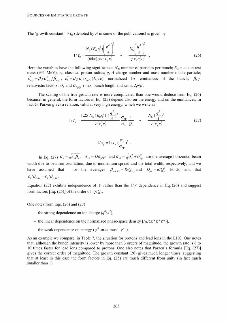
The ‘growth constant’ 01/τ (denoted by A in some of the publications) is given by

2 22 22

b 0 0 b

0 * * * * * *

( )1/

(64 ) x y x y

q qN E r NA A

τπ γ ε ε ε γ ε ε ε

⎛ ⎞ ⎛ ⎞⎜ ⎟ ⎜ ⎟⎝ ⎠ ⎝ ⎠= ∝ . (26)

Here the variables have the following significance: Nb, number of particles per bunch; E0, nucleon rest mass (931 MeV); r0, classical proton radius; q, A charge number and mass number of the particle;

* 2 *, , , / 0,x y x y x y l l p p ( / )E cε β γ σ β ε β γ σ σ Δ= = normalized 1 emittances of the bunch; σ ,β γ

relativistic factors; r.m.s. bunch length and r.m.s. Δp/p . Δ / and lσ σ p p

The scaling of the true growth rate is more complicated than one would deduce from Eq. (26) because, in general, the form factors in Eq. (25) depend also on the energy and on the emittances. In fact G. Parzen gives a relation, valid at very high energy, which we write as

2 22 2

b 0 0 bp* * * * * *

1.25 ( ) ( ) ( )11/ xx

xt xx y x y

q qN E r NA

Qσ

τσε ε ε ε ε ε

=

2

A∝ (27)

2p

p1/ 1/ ( )x

xx

στ τσ

= .

In Eq. (27) 2 2p p, / and px x x x xt x xD pσ ε β σ σ σ σ σ= = = + are the average horizontal beam

width due to betatron oscillation, due to momentum spread and the total width, respectively, and we have assumed that for the averages , av ,/x y x yR Qβ ≈ and 2

av / xD R Q≈ holds, and that

av av/ /x x y yε β ε β≈ .

Equation (27) exhibits independence of γ rather than the 1/γ dependence in Eq. (26) and suggest form factors [Eq. (25)] of the order of / . xQγ

One notes from Eqs. (26) and (27)

– the strong dependence on ion charge (q4/A2),

– the linear dependence on the normalized phase-space density [Nb/(εx*εy*εl*)],

– the weak dependence on energy ( 0γ or at most 1γ − ).

As an example we compare, in Table 7, the situation for protons and lead ions in the LHC. One notes that, although the bunch intensity is lower by more than 3 orders of magnitude, the growth rate is 6 to 10 times faster for lead ions compared to protons. One also notes that Parzen’s formula [Eq. (27)] gives the correct order of magnitude. The growth constant (26) gives much longer times, suggesting that at least in this case the form factors in Eq. (25) are much different from unity (in fact much smaller than 1).


263

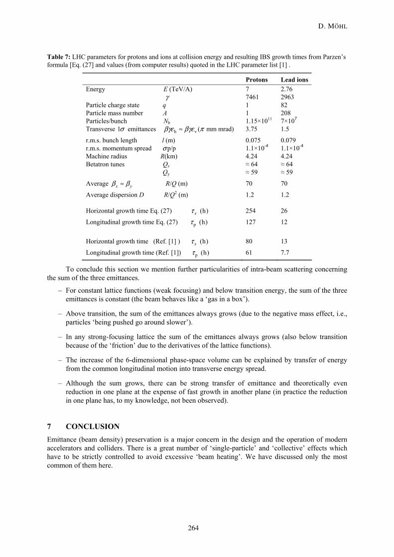
Table 7: LHC parameters for protons and ions at collision energy and resulting IBS growth times from Parzen’s formula [Eq. (27] and values (from computer results) quoted in the LHC parameter list [1] .

Protons Lead ions Energy E (TeV/A) 7 2.76 γ 7461 2963 Particle charge state q 1 82 Particle mass number A 1 208 Particles/bunch Nb 1.15×1011 7×107

Transverse 1 emittances σ h v ( mm mrad)βγε βγε π≈ 3.75 1.5

r.m.s. bunch length l (m) 0.075 0.079 r.m.s. momentum spread p/pσ 1.1×10-4 1.1×10-4

Machine radius R(km) 4.24 4.24 Betatron tunes Qx ≈ 64 ≈ 64 Qy ≈ 59 ≈ 59

Average x yβ β≈ R/Q (m) 70 70

Average dispersion D R/Q2 (m) 1.2 1.2 Horizontal growth time Eq. (27) (h)xτ 254 26

Longitudinal growth time Eq. (27) p (h)τ 127 12

Horizontal growth time (Ref. [1] ) (h)xτ 80 13

Longitudinal growth time (Ref. [1]) p (h)τ 61 7.7

To conclude this section we mention further particularities of intra-beam scattering concerning the sum of the three emittances.

– For constant lattice functions (weak focusing) and below transition energy, the sum of the three emittances is constant (the beam behaves like a ‘gas in a box’).

– Above transition, the sum of the emittances always grows (due to the negative mass effect, i.e., particles ‘being pushed go around slower’).

– In any strong-focusing lattice the sum of the emittances always grows (also below transition because of the ‘friction’ due to the derivatives of the lattice functions).

– The increase of the 6-dimensional phase-space volume can be explained by transfer of energy from the common longitudinal motion into transverse energy spread.

– Although the sum grows, there can be strong transfer of emittance and theoretically even reduction in one plane at the expense of fast growth in another plane (in practice the reduction in one plane has, to my knowledge, not been observed).

7 CONCLUSION Emittance (beam density) preservation is a major concern in the design and the operation of modern accelerators and colliders. There is a great number of ‘single-particle’ and ‘collective’ effects which have to be strictly controlled to avoid excessive ‘beam heating’. We have discussed only the most common of them here.

D. MOHL

264

Beam cooling (not treated in this note) can, to some extent, be used to fight emittance growth and even lead to very small equilibrium emittances. They result from the balance between the cooling and (many of) the heating mechanisms discussed above.

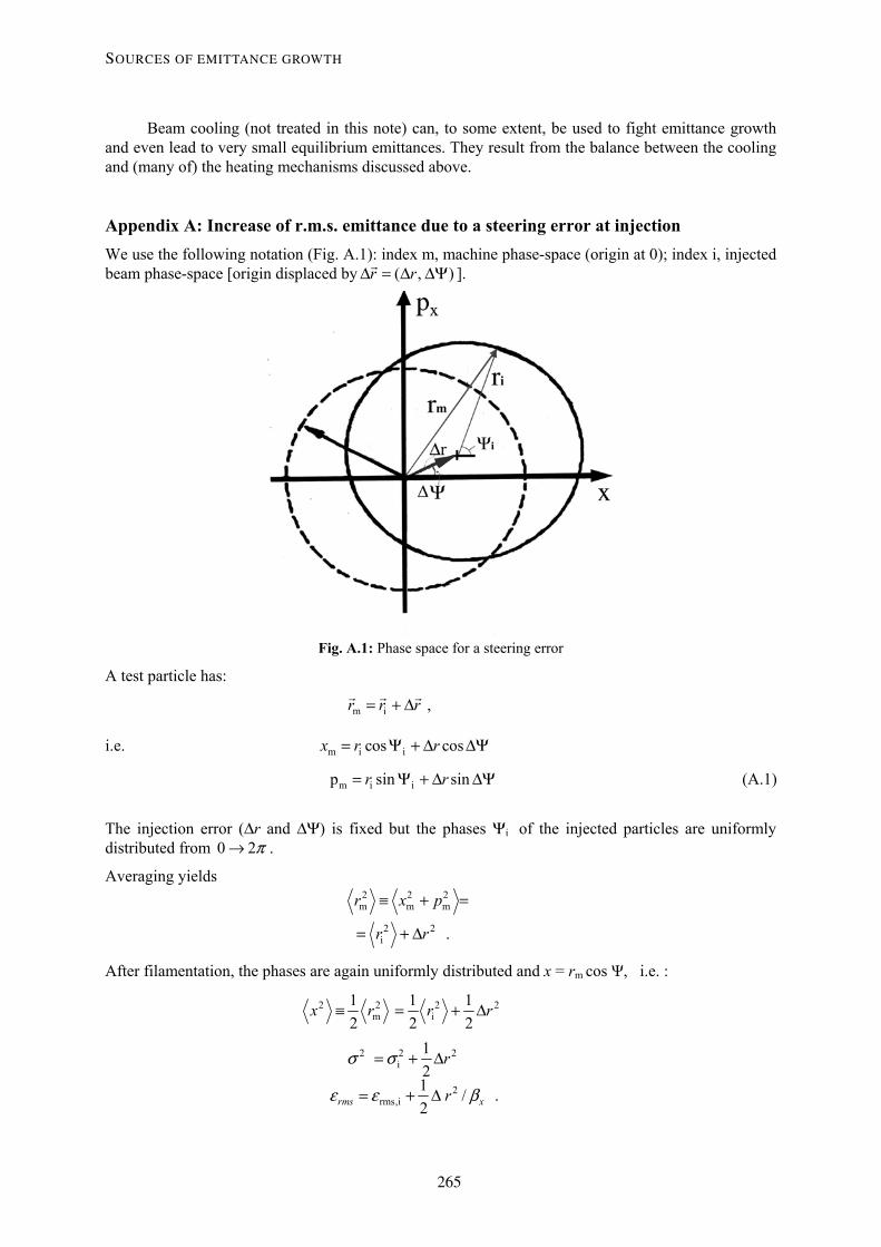
Appendix A: Increase of r.m.s. emittance due to a steering error at injection We use the following notation (Fig. A.1): index m, machine phase-space (origin at 0); index i, injected beam phase-space [origin displaced by ( , )r rΔ = Δ ΔΨ ].

Fig. A.1: Phase space for a steering error

A test particle has:

m i ,r r r= + Δ

i.e. m i icos cosx r r= Ψ + Δ ΔΨ

Ψm i ip sin sinr r= Ψ + Δ Δ (A.1)

The injection error (Δr and ΔΨ) is fixed but the phases Ψi of the injected particles are uniformly distributed from 0 2π→ .

Averaging yields 2 2 2

m m m

2 2i .

r x p

r r

≡ +

= + Δ

=

After filamentation, the phases are again uniformly distributed and x = rm cos Ψ, i.e. :

2 2 2 2m i

1 1 1 2 2 2

x r r≡ = + Δr

2 2i

12

rσ σ= + Δ 2

2rms,i

1 / 2rms xrε ε .β= + Δ


265

This result is derived and discussed in more detail in Refs. [2], [3], [26] and [27].

Appendix B: Increase of r.m.s. emittance due to mismatch of dispersion As before we assume that the machine has zero D, and the line has finite D, at the injection point; in the general case one has just to substitute the difference between line and machine and

D′ D′D D→ Δ

.D D′ ′→ Δ

For any particle:

i i i = cos( ) / , x r D p pΨ + Δ

i i i sin( ) ( ) /x x xp r D D p pβ α′= Ψ + + Δ .

For each value of Δp/p the phases Ψi are uniformly distributed around an off-momentum orbit with its centre displaced by i[ / , ( ) /x xr D p p D D p pi ].β α′Δ = Δ + After filamentation the phases are uniformly distributed around the origin Then [by virtue of Eqs. (3) above] 0.rΔ =

2 2 2 2i

1 = 2 xx A pσ =

and hence 2 2 2 2 2 2 2i i2 = { ( ) } ( / ) ,x x xx p r D D D p pσ β α′+ = + + + Δ

2 2 2 20 p

1{ ( ) }( /2 x x

2)D D D pσ σ β α σ′= + + +

2 2rms rms,i p 0

1 1 { ( ) }( / ) / )2 x xD D D pε ε β α σ σ⎡ ⎤′→ + + +⎢ ⎥⎣ ⎦

2 2 .

Appendix C: Increase of emittance due to β-function mismatch at transfer Consider the incoming beam (Fig. 9, above) in the normalized (circular) phase-space coordinates of a machine. To calculate the increase of the geometrical emittance, observe that after filamentation the incoming phase-space ellipse (containing a given fraction of the beam) fills the circumscribed circles of the machine phase-space. The increase in area and thus in geometrical emittance is b/a (major/minor ellipse axis):

% % ( / )b aε ε→ . (C.1)

To calculate the increase of the r.m.s. emittance as a function of b/a we can assume that the incoming beam ellipses are in the upright position (this amounts to rotating the normalized machine phase-space by a constant angle which does not affect the resulting blow-up). Then the coordinates of an incoming test particle can be written as

i r i, i r i/ sin / cosl lx A b a p A a bβ β= Ψ = Ψ .

Here is the single-particle emittance and the beam average 2iA 2 2

i 2 /x lA σ β= is [by virtue of Eqs. (2)

and (7) above] twice the r.m.s. emittance in the line. The coordinates xl, pl define the initial conditions for the circular phase-space motion with an amplitude in the ring. Averaging over all

particles assuming that the phases are random we find

2 2 2r ( l lr x p= + )

(2 2i r i/ / /r A b a a bβ = + ) / 2. This is (twice)

the r.m.s. emittance after filamentation in the ring. Thus the blow-up of the k r.m.s. emittance is

D. MOHL

266

( )/ /2k k s

b a a bσ σε ε

+→ . (C.2)

To express the aspect ratio b/a by the mismatch of the Twiss parameters we refer to Refs. [2] and [3] where it is shown that, in terms of the mismatch function F [Eq. (15) above],

( ) ( )2 21 , 1b aF F F Fa b

⎛ ⎞ ⎛ ⎞≡ + − = − −⎜ ⎟ ⎜ ⎟⎝ ⎠ ⎝ ⎠

.

From Eqs. (C.1) and (C.2) one then finds Eqs. (16) and (17) above for the blow-up of the geometrical and the r.m.s. emittance, respectively.

Appendix D: Increase of r.m.s. emittance due to scattering on a foil The normalized circular phase-space trajectories of a matched beam at the entrance of the foil are converted into elliptical trajectories at the exit (Fig. 12). In fact for any particle scattered by an angle θi

i i i0 i

i i i0 i 0 i

sin( )cos( ) (remember: ) .x x x

x x rp p p r p x xβ θ α β

→ = Ψ′→ + Δ = Ψ + = +

These are the initial conditions for the new betatron oscillation after the scattering event. Averaging over the beam, we take the phases Ψi of the original oscillation uniformly distributed and uncorrelated with the scattering angle. After filamentation in the line and/or the subsequent ring, the new betatron phases are also uniformly distributed and one obtains

2 2 2 2 2 2i i i i0 0 i

2 2 2 2 2 20 0 rms 0 0 rms

p

12 2 or ( ) / ( )2

x

x x k x k

r x r

k kσ σ

β θ

σ σ 0β θ ε σ β ε θ β

= + = +

→ = + = =

Thus the blow-up of emittance is kσ

2rms 0

1 ( )2k kσε θ βΔ = .

We have tacitly assumed above that the beta function is the same at the entrance and exit so that the beam remains matched in the absence of the scatterer. By re-adjusting the optics in the downstream part of the line, the blow-up can in fact be somewhat reduced. The idea is to provide a smaller β function 1 0( )β β< at exit (1) than at the entrance (0) of the scatterer. For simplicity, we perform the calculation only for . We chose 0α = 1β such that it matches the ellipse in Fig. 12 (right) after scattering instead of the circumscribed circle. This is called re-matching at the scatterer. Then, for any particle

0 0 0 1 1 1

0 0 0 1 1 1

cos( ) cos( )

1/ sin( ) 1/ sin( ) .

x A A

x A A

β β

β θ β

= Ψ = Ψ

′ = − Ψ + = − Ψ

Taking the squares and averaging with the assumption that the beam remains matched before and after the foil (so that all the cos2 and sin2 terms average to 1/2), one obtains


267

2 20 0 1 12

2 20 12

0 1

2 2

.2 2

A Ax

A Ax

β β

β β

= =

′ = =

The solution of this system is 2 22 2

1 0 0 rms

2012

0 1

2

.

A A A

A

A

β θ

ββ

− =

=

20

Remember that the 1 emittance isσ 2rms / 2.Aε = Therefore one obtains

22 20 rms 0 rms 0 rms

1 0 00 0

1 11 12 8

β θ β θ β θε ε εε ε

2

0ε

⎧ ⎫⎛ ⎞⎪ ⎪= + ≈ + − ⎜ ⎟⎨ ⎬⎜ ⎟⎝ ⎠⎪ ⎪⎩ ⎭

12

0 0 rms

0

1

1

ββ β θ

ε

=

+

.

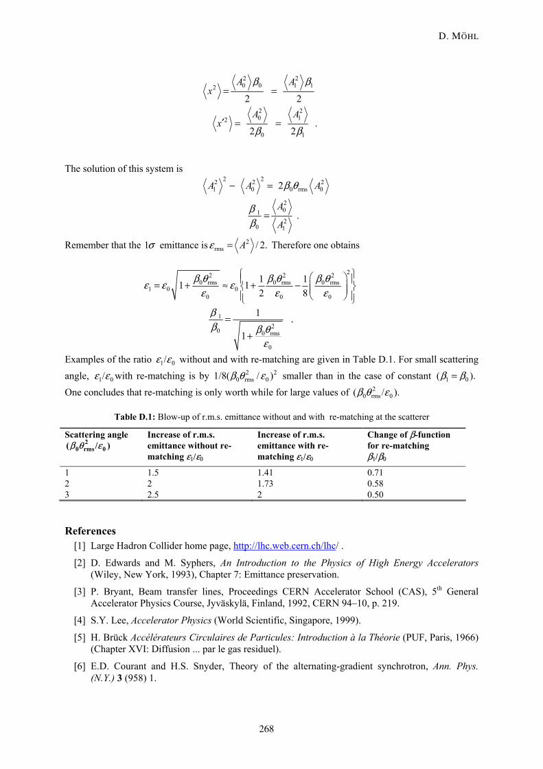
Examples of the ratio without and with re-matching are given in Table D.1. For small scattering angle, with re-matching is by

1 0/ε ε

1 0/ε ε 20 rms 01/8( / )2β θ ε smaller than in the case of constant 1 0( ).β β=

One concludes that re-matching is only worth while for large values of 20 rms 0( / ).β θ ε

Table D.1: Blow-up of r.m.s. emittance without and with re-matching at the scatterer

Scattering angle 2

0 rms 0( / )β θ ε Increase of r.m.s. emittance without re-matching ε1/ε0

Increase of r.m.s. emittance with re- matching ε1/ε0

Change of β-function for re-matching β1/β0

1 1.5 1.41 0.71 2 2 1.73 0.58 3 2.5 2 0.50

References [1] Large Hadron Collider home page, http://lhc.web.cern.ch/lhc/ .

[2] D. Edwards and M. Syphers, An Introduction to the Physics of High Energy Accelerators (Wiley, New York, 1993), Chapter 7: Emittance preservation.

[3] P. Bryant, Beam transfer lines, Proceedings CERN Accelerator School (CAS), 5th General Accelerator Physics Course, Jyväskylä, Finland, 1992, CERN 94–10, p. 219.

[4] S.Y. Lee, Accelerator Physics (World Scientific, Singapore, 1999).

[5] H. Brück Accélérateurs Circulaires de Particules: Introduction à la Théorie (PUF, Paris, 1966) (Chapter XVI: Diffusion ... par le gas residuel).

[6] E.D. Courant and H.S. Snyder, Theory of the alternating-gradient synchrotron, Ann. Phys. (N.Y.) 3 (958) 1.

D. MOHL

268

[7] H. Grote, F. Iselin, The MAD program (Methodical Accelerator Design), version 8.10: User’s reference manual, CERN-SL-90-13-AP-rev-3 and version 9.01: http://project-mad9.web.cern.ch/project-mad9/mad/mad9/conversion/ .

[8] J. Rossbach and P. Schmüser, Basic course on accelerator optics, Proceedings CERN Accelerator School (CAS), 5th General Accelerator Physics Course, Jyväskylä, Finland, 1992, CERN 94–01, p. 17.

[9] E.J.N. Wilson, Nonlinear resonances, Proceedings CERN Accelerator School (CAS), 5th Advanced Accelerator Physics Course, Rhodes, Greece, 1993, CERN 95–06, p. 15.

[10] E. Keil, W. Schnell and P. Strolin, Feedback damping of horizontal beam transfer errors, CERN 69–27 (1969).

[11] L. Vos, Damping of coherent oscillations, internal report CERN-SL-96-066-AP.

[12] Particle Data Group, Review of particle physics, Eur. Phys. J. 3 (1998) 144. (Chapter 23, Passage of particles through matter).

[13] L. Durieux et al., A low-β insertion in the PS SPS transfer line, internal report CERN/PS 2001–06 (AE).

[14] S. Baird et al., Machine aspects for LEAR operation with JETSET, Proc. 4th LEAR Workshop, Villars-sur-Ollon, 1987 (Harwood Academic Publishers, Chur, 1988), p. 91.

[15] W. Hardt, A few simple expressions for checking vacuum requirements in proton synchrotrons, internal report CERN ISR-300/GS/68-11.

[16] A. Wrulich, Single beam lifetime, Proceedings CERN Accelerator School (CAS), 5th General Accelerator Physics Course, Jyväskylä, Finland, 1992, CERN 94–01, p. 409.

[17] B. Oksendal, Stochastic Differential Equations (Springer, Berlin, 1992).

[18] H.G. Hereward and K.Johnsen, The effect of radio-frequency programme noise on the phase-stable acceleration process, CERN 60–38 (1960).

[19] G. Dome, Diffusion due to RF-noise, Proceedings CERN Accelerator School (CAS), Advanced Accelerator Physics Course, Oxford, 1985, CERN 87–03, p. 370.

[20] A. Piwinski, Intra-beam scattering, Proceedings 9th Int. Conf. on High Energy Accelerators, Stanford, 1974 (AEC, Washington D.C., 1974) CONF 740522, and Proceedings CAS - CERN Accelerator School, 4th Advanced Accelerator Physics Course, Noordwijkerhout, Netherlands, 1991, CERN 92–01, p. 226.

[21] A.H. Sorensen, Introduction to intrabeam scattering, Proceedings CAS - CERN Accelerator School, General Accelerator Physics Course, Aarhus, Denmark, 1986, CERN 87–10, p. 135.

[22] A. Piwinski, Touchek effect and intra-beam scattering, in Handbook of Accelerator Physics, A. Chao and M. Tigner, eds. (World Scientific, Singapore, 1998), p. 125.

[23] G. Parzen, Intrabeam scattering at high energies, Nucl. Instrum. Meth., A256 (1987) 231.

[24] M. Martini and T. Risselada, Comparison of intra-beam scattering calculations, internal report CERN/SL/Note 94-80 (AP).

[25] J.D. Bjorken and S.K. Mtingwa, Intrabeam scattering, Part. Accel. 13 (1983) 115.

[26] P.M. Hanney and E. Keil, How do angle and position at injection error affect beam size and beam density?, internal report CERN ISR-TH/GS/69-44.

[27] H.G. Hereward, How good is the r.m.s. as a measure of beam size, internal report CERN MPS/DL 69-15.


269

Documents

SOURCES OF EMITTANCE GROWTH - cds.cern.ch · SOURCES OF EMITTANCE GROWTH D. Möhl CERN, Geneva, ... For hadrons, i.e., proton and ion beams, the geometri cal emittance is appropriate