Some Theoretical and Practical Perspectives of the Travel

Some Theoretical and Practical Perspectives of the Travel Time

Kinematic Wave Model: Generalized Solution, Applications,

and Limitations

Peter J. Jina∗ Ke Hanb† Bin Ranc‡

aDepartment of Civil, Architectural, and Environmental EngineeringUniversity of Texas at Austin, Austin, TX 78701, USA

bDepartment of MathematicsPennsylvania State University, University Park, PA 16802, USA

cDepartment of Civil and Environmental EngineeringUniversity of Wisconsin-Madison, Madison, WI 53706, USA

Submitted for presentation at the 93rd Annual Meeting of Transportation Research Board,January, 2014

Word count based on Latex: 5328 words + 7 figures + 1 table = 7328

Abstract

This paper explores the travel time kinematic wave (KW) model recently-reveal throughHamilton-Jacobi (H-J) Partial Differential Equation (PDE) theory proposed by Laval andLeclercq. We focus on theoretical and practical aspects of the travel time KW modelin real-world traveler information and traffic management applications. The travel timekinematic wave (KW) model is an equivalent representation of the Lighthill-Whitham-Richards (LWR) model. The model preserves both the spatial representation in Eulermodel and the numerical and formulation benefits in Lagrangian model, making it suitablefor conducting traffic state estimation based on prevailing mobile sensor data such as GPS,cellular, and Bluetooth probe data. In this paper, we provide an in-depth discussion on thephysical meaning of the model revealed through a heuristic derivation of the travel timeKW model and the rigorous proof of its requivalenso to the other two Euler and Lagrangianmodel. We extend the Lax-Hopf formulations and solution methods proposed in Lavaland Leclercq’s study to account for internal boundary problems that may be used toformulating signalized intersection, active traffic management, and the emerging connectedvehicle data. Meanwhile, by comparing the two Lagrangian formulations of LWR withrespect to vehicle sinks and sources, route-based, and lane-based applications, we attemptto provide a realistic perspective on the potentials and challenges facing Lagrangian trafficflow models.Keywords: macroscopic traffic flow model, Lagrangian coordinate, probe vehicle tech-nologies

∗Corresponding author, Tel: +1 512-232-3124. E-mail address: [email protected]†E-mail: [email protected]‡E-mail:[email protected]

1

TRB 2014 Annual Meeting Paper revised from original submittal.

1 Notations

n: number of vehicles, the order of a vehicle after a reference vehicle, Lagrangian coordinate.x: location, distance on a road.t: time, duration.k: density, k = −nx (where nx represents the partial derivative of n over x)q: flow, q = ntu: speed, u = xth: distance headway between two vehicles, h = −xn, h = 1/k.τ : travel time density, travel time over a unit distance, τ = tx, and τ = 1/u.p: time headway between two vehicles, p = tn and p = 1/q.

2 Introduction

The first-order vehicular conservation model (LWR model) proposed by Lighthill and Whitham(1955) and Richards (1956) has been the foundation of the continuum traffic flow theory. Itis the most widely-used macroscopic traffic flow model, particularly after Daganzo’s seminalwork on the cell transmission model that solves the LWR model efficiently at large scales.One key benefit of LWR model is that traffic data from traditional fixed-location detectors(e.g. loop detectors) can be efficiently plugged into the model for traffic state estimation andprediction. Over the last decade, the probe vehicle technologies such as GPS, cellphone, andBluetooth probe vehicle technologies have experienced rapid development and deployment andbecome a key data source in traveler information provision. Traffic data collected from mobilesensor technologies have different characteristics than the fixed-location sensor data. Thedata is usually collected with individual vehicles rather than at fixed-location at fixed timeintervals. The data usually relies on complicated data processing techniques to fix the space-time models which can lead to unreliable estimation results especially with sampling error anddata noises. Under such background, Lagrangian coordinate based traffic flow models start toattract the attention of both traffic flow theorists and modelers. The Lagrangian coordinatewas first introduced into traffic flow from hydrodynamics by Moskowitz (1965) and elaboratedby Makigami et al. (1971). In hydrodynamics, the Lagrangian coordinate is defined as thefollowing.

n (x, t) = −∫ x

x(t)k (s, t) ds (2.1)

The equivalent traffic flow definition is found to be the order of vehicles with preceding vehiclesalways have smaller Lagrangian coordinate than following vehicles. It should be noted thatthis coordinate does not stick to a physical vehicle. In multi-lane situation when vehicle passesone another their vehicle orders will switch.

Figure 1 illustrates the physical meaning of Lagrangian coordinate. In the vehicular coor-dinate, the origin can be a selected reference vehicle and the coordinate does not stick withphysical vehicles. When one vehicle passing the other vehicle in a multi-lane segment, theirvehicular coordinates switches as illustrated with the yellow and green vehicles. The vehicularcoordinate, in the form of accumulative vehicles at a cross section, has been widely used instudying traffic flow characteristics and highway capacity (Banks, 1990, 1991; Cassidy andBertini, 1999; Cassidy and Windover, 1995). The concept also leads to the development ofthe Variational Theory for traffic flow first proposed by Luke (1972) and Newell (1993a, b, c),and completed by Daganzo (2005a, b).

2


Identical Vehicle

9 8 7 6 5 4 3 2 1 0 -1 -2 -3 -4

I I I I I I I I I I I I I I9 8 7 6 5 4 3 2 1 0 -1 -2 -3 -4

I

n

Direction of Traffic

9 8 7 6 5 4 3 2 1 0 -1 -2

I I I I I I I I I I I II9 8 7 6 5 4 3 2 1 0 -1 -21

1 10

n

I

Figure 1: Illustration of the Lagrangian Coordinate. Notice that the coordinates are changedwhen the yellow vehicle overtakes the green vehicle.

Lagrangian coordinate can be incorporated into the continuum traffic flow modelling intwo different ways. The first one is to establish moving boundary conditions for the Eulerformulations using measurements over the Lagrangian coordinate (Claudel and Bayen, 2010a,b; Herrera and Bayen, 2010). The other one is to use the Lagrangian coordinate similarto the Lagrangian formulation in the hydrodynamics. Leclercq et al. (2007) first studiedthe hydrodynamic Lagrangian model under the context of traffic flow theory. It is foundthat the Lagrangian model with respect to vehicle and time can be derived by using a spacefunction based variational theory. The model exhibits some significant numerical advantagesover the original space-time model for problems with respect to moving coordinates, e.g.moving bottlenecks. Furthermore, the solution of Godunov scheme converges to an upwindscheme under a triangular fundamental diagram for the Lagrangian formulation. Lagrangiancoordinate can also be used to reformulate multi-class models (van Wageningen-Kessels etal., 2010), network models (van Wageningen-Kessels et al., 2013), and high-order traffic flowmodels such as Aw-Rascle models (Moutari and Rascle, 2007).

The travel time kinematic wave (KW) model is revealed by the Hamilton-Jacobi theoryrecently proposed by Laval and Leclerq (2013). By defining a traffic flow surface with respectto three two-dimensional coordinate systems, the HJ formulation can be applied to derivethe existing Euler (LWR Model) and Lagrangian-time model, as well as the Lagrangian-spaceTravel Time KW model. The paper further derive the Lax-Hopf boundary formulations forpiece-wise linear empirical support and rectangular boundary problems. With the theoreticalfoundation profoundly established by Laval and Leclerq (2013)’s work, this paper attemps toinvestigate the practical perspectives regarding the physical meaning of the new model, itsrelationship to the other two models, and the model implementation in real-world travelerinformation and traffic management applications. We identified and proposed a Lax-Hopf

3


framework for the missing irregular boundary problem formulations so that the model can beused in practice to model signalized intersection, freeway control strategies, and the emergingconnected vehicle data sources. We discussed the limitations of the model with respect tovehicle sinks and sources and in lane-based applications.

3 Physical Aspects of The Travel Time Kinematic Wave (KW)Model

3.1 The heuristic derivation of the travel time KW model

The travel time KW model can be derived by considering a single-lane road section with twopaired vehicle tracking stations that can measure the vehicle travel times on the road section.The two detectors are located at x and x + ∆x as shown in Figure 2. We investigate twoconsecutive groups of ∆n vehicles with their leading vehicles being nth and (n+∆n)th vehiclein the traffic stream respectively. The total travel time for each vehicle group to pass throughthe road section are t and t + ∆t respectively. The temporal headway changes from p in thefirst group to p+ ∆p in the second group, then ∆t can be written as

∆t = (p+∆p) ∆n− p∆n = ∆p∆n (3.2)

If we define the travel time ratio τ as the inverse of the space mean speed of a vehiclegroup, ∆t can also be interpreted as the changes of the travel time ratio on the segment. Thetravel time ratio is assumed to be τ when the first vehicle group starts to exit the section;while it changes to τ + ∆τ when the second vehicle group starts to exit, then ∆t can also becalculated as the following.

∆t = (τ+∆τ) ∆x−τ∆x = ∆τ∆x (3.3)

x x+Dx

t

t+Dt

nn+Dn

p+Dp

p

t (n) = t

t (n+Dn) = t + Dt

Figure 2: Physical Derivation of the Travel Time KW Model

Since Equations (3.2) and (3.3) describe the same quantity, we have

∆t = ∆p∆n = ∆τ∆x. (3.4)

Thus, the differencing formulation can be obtained for the travel time KW model as thefollowing

∆p

∆x−∆τ

∆n= 0 (3.5)

4


Considering all the medium are continuous including vehicle numbers and allowing the incre-ment to be infinitesimal, it follows that

τn−px = 0 (3.6)

This section mainly focuses on interpretting the physical meaning of the travel time KWmodel. More rigorous derivation based on variational theory and Hamilton-Jacobi theory canbe found in Laval and Leclerq (2013).

3.2 Godunov Numerical Scheme

The proposed model is a typical nonlinear first-order hyperbolic conservation equation. Itssolution can be obtained by the characteristic method and the Rankine–Hugoniot condition.The slope of the shock boundary between two states (p1, τ1) and (p2, τ2) in the n-x diagramcan be obtained as the following.

snx = −p1−p2

τ1−τ2=

p2−p1

τ1−τ2(3.7)

In the travel time KW model, the slope of the shock wave boundary means the changingrate of the shock boundary caused by each unit vehicle switching between the vehicle groupsat both sides of the shock. Meanwhile, the solutions from the proposed model are equivalentto the corresponding LWR and Lagrangian model even with source term and in weak sense.Godunov scheme can be used to solve the travel time KW model efficiently. Considering a nu-merical grid with a resolution of ∆n and ∆x for Lagrangian and space coordinate respectively.Then the Godunov scheme can be written as the following.

Tn+∆nx = Tnx +

∆n

∆x

[p(Tnx , T

nx+∆x

)−p(Tnx−∆x, T

nx

)](3.8)

where Tnx denotes the average τ values obtained for the grid at (n, x), p is a function to beobtained when solving the Riemann problem (See the Godunov Procedure listed at the end ofthis section), given the travel time ratio experienced by the previous vehicle group on the roadsection x and its downstream section at (x+∆x). Meanwhile, the CFL (Courant-Friedrichs-Lewy) condition (Courant et al., 1967) for the travel time KW model over the rectangle gridson the n-x diagram is as the following.∣∣∣∣∆n∆x

∣∣∣∣ ≤ ∣∣∣∣ 1

p′ (τ)

∣∣∣∣ (3.9)

The above CFL condition can be implemented in two ways. When fixing the size of thevehicle group which can be constrained by the sampling rate of a particular vehicle detectiontechnologies, we divided road segments equivalent to its maximal characteristic spacing (e.g.free flow spacing), that is,

∆x ≥∣∣p′(τ)

∣∣max

∆n (3.10)

The other way is to fix the segment length required by ATIS (Advanced Traveler InformationSystem) applications, then the CFL condition can be used to determine the number of vehicles∆n to be processed at each numerical iteration.

∆n ≤ ∆x

|p′(τ)|max(3.11)

5


The fixed ∆n method can ensure the estimation accuracy but it can lead to large ∆x thatare meaningless for ATIS applications. Even though the sample size may not be sufficient tosupport traffic state estimation at every segment, the fixed ∆x method are more flexible for 1)tuning the resolution of the Lagrangian coordinate and 2) the implementation of pre-definedATIS reporting spatial resolutions. Furthermore, by fixing the segment length, the numericalmethod can incorporate the segment based representation used in numerical methods forLWR model while still allowing flexibility in adjusting the resolution of the solutions on theLagrangian coordinate.

q

k0

p

0 t

Free-flow

Congested

Free-flow

Congested

C

1/C

h1 hC

(a) (b)

(c)

u

h0

Free-flow

Congested

hjam

Figure 3: Triangular q-k and p-τ diagram, Shock waves in n-x diagram

In Daganzo’s cell transmission model (Daganzo, 1994), the triangular flow-density rela-tionship is introduced to reduce the infinitely many directions of characteristics with continu-ous FDs to only two or three directions depending on the capacity constraint. It substantiallyreduces the complexity of the Godunov scheme which leads to highly-efficient numerical meth-ods. Triangular FD can also simplify the Godunov scheme for the travel time kinematic wavemodel. Figure 3 (a,b) compares the geometric characteristics between the triangular q-k andp-τ diagram. In triangular FDs, the free-flow regime only has one uniform speed which cor-responds to a vertical line on the p-τ diagram; while the congested regime in p-τ diagram islinear. If a capacity constraint is added, the p-τ diagram is then cut-off at the bottom creatinga saturated regime with time headway of 1/C (where C is the capacity).In the following, the Godunov based numerical methods for the proposed travel time KWmodel are summarized.

6


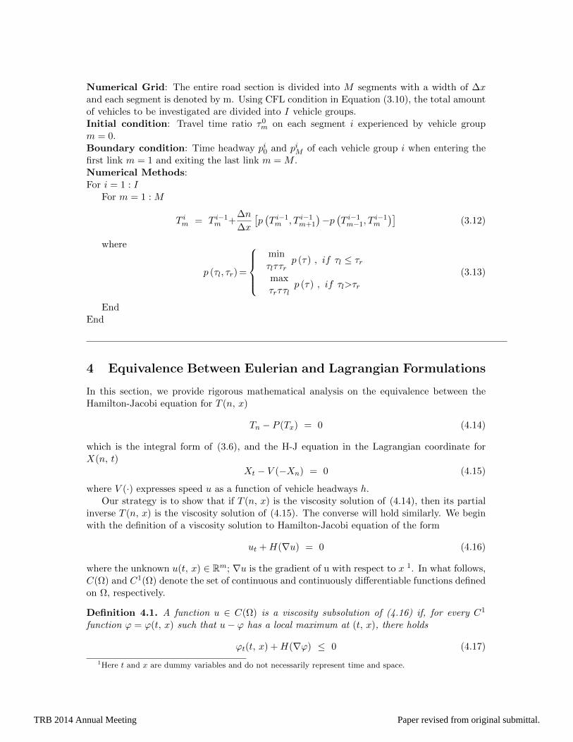
Numerical Grid: The entire road section is divided into M segments with a width of ∆xand each segment is denoted by m. Using CFL condition in Equation (3.10), the total amountof vehicles to be investigated are divided into I vehicle groups.Initial condition: Travel time ratio τ0

m on each segment i experienced by vehicle groupm = 0.Boundary condition: Time headway pi0 and piM of each vehicle group i when entering thefirst link m = 1 and exiting the last link m = M .Numerical Methods:For i = 1 : I

For m = 1 : M

T im = T i−1m +

∆n

∆x

[p(T i−1m , T i−1

m+1

)−p(T i−1m−1, T

i−1m

)](3.12)

where

p (τl, τr) =

minτlττr

p (τ) , if τl ≤ τr

maxτrττl

p (τ) , if τl>τr

(3.13)

EndEnd

4 Equivalence Between Eulerian and Lagrangian Formulations

In this section, we provide rigorous mathematical analysis on the equivalence between theHamilton-Jacobi equation for T (n, x)

Tn − P (Tx) = 0 (4.14)

which is the integral form of (3.6), and the H-J equation in the Lagrangian coordinate forX(n, t)

Xt − V (−Xn) = 0 (4.15)

where V (·) expresses speed u as a function of vehicle headways h.Our strategy is to show that if T (n, x) is the viscosity solution of (4.14), then its partial

inverse T (n, x) is the viscosity solution of (4.15). The converse will hold similarly. We beginwith the definition of a viscosity solution to Hamilton-Jacobi equation of the form

ut +H(∇u) = 0 (4.16)

where the unknown u(t, x) ∈ Rm; ∇u is the gradient of u with respect to x 1. In what follows,C(Ω) and C1(Ω) denote the set of continuous and continuously differentiable functions definedon Ω, respectively.

Definition 4.1. A function u ∈ C(Ω) is a viscosity subsolution of (4.16) if, for every C1

function ϕ = ϕ(t, x) such that u− ϕ has a local maximum at (t, x), there holds

ϕt(t, x) +H(∇ϕ) ≤ 0 (4.17)

1Here t and x are dummy variables and do not necessarily represent time and space.

7


Similarly, u ∈ C(Ω) is a viscosity supersolution of (4.16) if, for every C1 function ϕ = ϕ(t, x)such that u− ϕ has a local minimum at (t, x), there holds

ϕt(t, x) +H(∇ϕ) ≥ 0 (4.18)

We say that u is a viscosity solution of (4.16) if it is both a supersolution and a subsolutionin the viscosity sense.

Remark 4.2. If u is a C1(Ω) function and satisfies (4.16) at every x ∈ Ω, then u is also asolution in the viscosity sense. Conversely, if u is a viscosity solution, then the equality musthold at every point x where u is differentiable. In particular, if u is Lipschitz continuous, thenit is almost everywhere differentiable, hence (4.16) holds almost everywhere in Ω.

The next theorem establishes the equivalence between viscosity solutions of (4.14) and(4.15).

Theorem 4.3. Assume that T (n, x) is a viscosity solution of (4.14). Furthermore, assumethat T (n, x) is Lipschitz continuous in x, that is, for some L > 0,

1

v0|x1 − x2| ≤ |T (n, x1)− T (n, x2)| ≤ L |x1 − x2| ∀x1, x2, ∀n

where v0 denotes the free-flow speed. Then one can partially invert T (n, x) and get X(n, t),which is a viscosity solution to (4.15).

Proof. According to our assumption, X(n, t) is strictly decreasing in t with

1/L |t1 − t2| ≤ |X(n, t1)−X(n, t2)| ≤ v0 |t1 − t2| ∀ t1, t2, ∀n (4.19)

We start by showing that X(n, t) is a subsolution. Indeed, given any C1 function Y = Y (n, t)such that X − Y has a local maximum at (n0, t0). Without loss of generality, we assumeX(n0, t0)− Y (n0, t0) = 0. We consider the plane n = n0, see Figure 4.

n = n0 t0

Y(n , )0.

t

x

n

0.X(n , )

Figure 4: Graphs of X(n0, ·) and Y (n0, ·)

Since X − Y attains a local maximum at (n0, t0), by (4.19) there must hold Yt(n0, t0) < 0.By continuity, there exists a neighborhood Ω1 of (n0, t0) such that Yt(n, t) < 0, ∀(n, t) ∈ Ω1.Then we may define T (n, ·) to be the inverse of Y (n, ·) in Ω1. Obviously, T (n, t) ∈ C1(Ω1),and T − T attains a local maximum at

(n0, X(n0, t0)

). Using the fact that T (n, x) is a

viscosity solution and applying (4.17), we deduce

Tn(n, x)− P(Tx(n, x)

)≤ 0 (4.20)

8


Differentiating with respect to n the identity Y(n, T (n, x)

)= x and using (4.20), we have

0 = Yn + Yt Tn ≥ Yn + Yt P (Tx) = Yn + Yt P

(1

Yt

)(4.21)

In the above deduction, we have used the technique of differentiating both sides of Y (n, T (n, x)) ≡x with respect to x and obtaining 1 = Yt ·Tx. Finally according to (4.21) and the monotonicityof the function V (·), we deduce

−Yn ≥ YtP(

1

Yt

)=⇒ V (−Yn) ≥ V

(YtP

(1

Yt

))= Yt

we thus conclude that Yt − V (−Yn) ≤ 0. Since Y is arbitrary, X(n, t) must be a subsolution.The case for supersolution is completely similar.

5 Lax-Hopf Formula with Internal Boundary Conditions

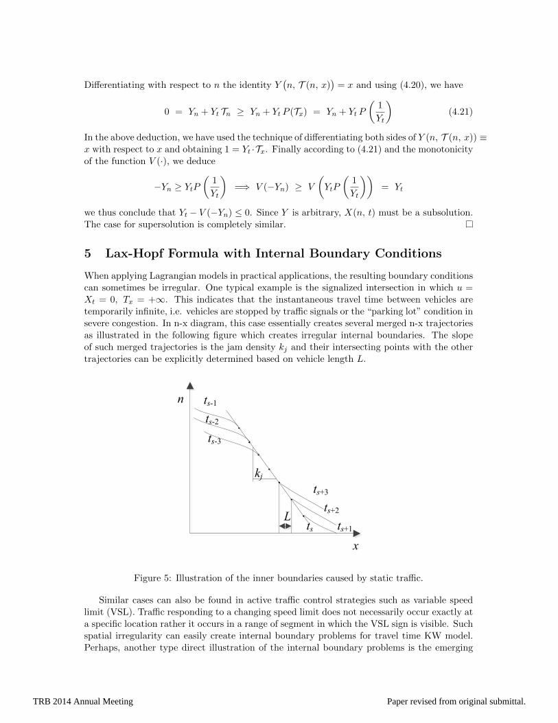
When applying Lagrangian models in practical applications, the resulting boundary conditionscan sometimes be irregular. One typical example is the signalized intersection in which u =Xt = 0, Tx = +∞. This indicates that the instantaneous travel time between vehicles aretemporarily infinite, i.e. vehicles are stopped by traffic signals or the “parking lot” condition insevere congestion. In n-x diagram, this case essentially creates several merged n-x trajectoriesas illustrated in the following figure which creates irregular internal boundaries. The slopeof such merged trajectories is the jam density kj and their intersecting points with the othertrajectories can be explicitly determined based on vehicle length L.

kj

L

n

x

ts-3

ts-1

ts

ts-2

ts+1

ts+2

ts+3

Figure 5: Illustration of the inner boundaries caused by static traffic.

Similar cases can also be found in active traffic control strategies such as variable speedlimit (VSL). Traffic responding to a changing speed limit does not necessarily occur exactly ata specific location rather it occurs in a range of segment in which the VSL sign is visible. Suchspatial irregularity can easily create internal boundary problems for travel time KW model.Perhaps, another type direct illustration of the internal boundary problems is the emerging

9


connected vehicle data sources. Vehicles with DSRC (Dedicated Short Range Communication)devices can simulatenously broadcast their locations to other vehicles or roadside sensors tobe used in safety and mobility applications. When plotting such data onto the n-x diagram,we essentially obtain time trajectories. Each point in a time trajrectory represents the nthvehicle located at x location at the time of ”snapshot” forming irregular internal boundaries.

In this section, we present a generalized Lax-Hopf formula for the H-J equation (4.14) withinternal (irregular) boundary conditions, following the viability theory and solution represen-tation proposed by Aubin et al. (2008). The articulation of the generalized Lax-Hopf formularequires the following definition of value conditions.

Definition 5.1. Given a lower-semicontinuous function D(·, ·) that maps Ω, a subset of R2,to R. The value condition C(·, ·) is defined as

C(n, x) =

D(n, x) (n, x) ∈ Ω

+∞ (n, x) /∈ Ω

For simplicity, let us consider a piecewise affine (PWA) Hamiltonian H(τ).= −p(τ) depicted

in the left part of Figure 6. Define the concave transformation of the Hamiltonian:

L(u) = supτ∈[1/ufree,+∞)

− p(τ)− uτ

= p∗ − uτ∗ u ∈ [−w, k] (5.22)

Theorem 5.2. (Generalized Lax-Hopf formula) The viability episolution to (4.14) asso-ciated with value condition C(·, ·) is given by

TC(n, x) = inf(u, τ)∈Dom(L)×R+

C(n− τ, x− τu) + τL(u)

(5.23)

Proof. Formula (5.23) is the Lax-Hopf formula (Aubin et al., 2008) stated for the H-J equation(4.14).

1/ufree

p*

τ∗

x1

x2

n n21

x

x1

2

n n1 2

k

−w

p

τ

n

x

n

x

I

II

III

r

k

−w

k

I

II

III

−w

r

Figure 6: Left: the piecewise affine Hamiltonian. Middle: partition of the domain of depen-dence into three parts when r ∈ [−w, k]. Right: partition of the domain of dependence intothree parts when r < −w or r > k.

The viability episolution in (5.23) has an important property stated below (Aubin et al.,2008)

Proposition 5.3. (inf-morphism property) Let C(·, ·) be the minimum of finitely manyvalue conditions,

C(n, x).= min

i=1,...,mCi(n, x)

10


ThenTC(n, x) = min

i=1,...,mTCi(n, x) (5.24)

The inf-morphism property allows the H-J equation with multiple complex value conditionsto be decomposed into several problems each with a single value condition. Such propertytremendously simplifies solution representation and computation.

5.1 Piecewise Affine Internal Boundary Conditions

We consider piecewise affine (PWA) internal boundary conditions and note that any internalboundary condition with irregular domain can be approximated by PWA conditions. Per ourprevious discussion on the inf-morphism property, it suffices to state the Lax-Hopf formulafor the simplest internal value conditions, that is, the affine ones. Piecewise affine and morecomplex conditions can be handled by taking the lower envelop of solutions with simple affinevalue conditions.

Theorem 5.4. (Lax-Hopf formula for affine internal boundary condition) Given realnumbers x1, x2, n1, n2, assume that the domain of the affine internal condition Ω is a linesegment with end points (n1, x1) and (n2, x2). Let r = (x1 − x2)/(n1 − n2). In addition,assume that the affine internal condition satisfies

Cint(n, x) = β + α (n− n1) (n, x) ∈ Ω (5.25)

With the piecewise affine Hamiltonian depicted in Figure 6, the generalized Lax-Hopf formula(5.23) can be instantiated as follows.(1). If r ∈ [−w, k],

Tint(n, x) =

β + α(x1 − n1r − x+ nk

k − r− n1

)+−x1 + n1r + x− nr

k − r(p∗ − kτ∗)

if

x− x2 ≥ k (n− n2),

x− x1 ≤ k(n− n1),

x− x1 ≥ r(n− n1).

Region I

β + α

(x− x1 + rn1 + wn

r + w− n1

)+−x+ x1 − rn1 + nr

r + w(p∗ + wτ∗)

if

x− x2 ≤ −w(n− n2),

x− x1 ≥ −w(n− n1),

x− x1 < r(n− n1).

Region II

β + α(n2 − n1) + (n− n2)

(p∗ − x− x2

n− n2τ∗)

ifx− x2 < k(n− n2),

x− x2 > −w(n− n2).

Region III

(5.26)

11


(2). If r < −w or r > k,

Tint(n, x) =

A if

x− x2 ≤ k (n− n2),

x− x1 ≥ k(n− n1),

x− x2 ≥ −w(n− n2).

Region I

B if

x− x2 ≤ −w(n− n2),

x− x1 ≥ −w(n− n1),

x− x1 ≤ k(n− n1).

Region II

minA, B if

x− x2 < −w(n− n2),

x− x1 > k(n− n1),

x− x2 ≥ r(n− n2).

Region III

(5.27)

where

A.= β + α

(kn− x− rn2 + x2

k − r− n1

)+x+ rn2 − x2 − nr

k − r(p∗ − kτ∗) (5.28)

B.= β + α

(wn+ x+ rn2 − x2

r + w− n1

)+rn− x− rn2 + x2

r + w(p∗ + wτ∗) (5.29)

Proof. In either case (1) or case (2), the domain of dependence can be partitioned into threedisjoint regions I, II and III according to the admissible wave speeds k and −w, see the middleand right parts of Figure 6 for an illustration. Notice that in both cases, the minimum-costpath for region I is a line segment with slope k; while the minimum-cost path for region II is aline segment with slope −w. In region III of case (1), the minimum-cost path is the segmentconnecting (n, x) and (n2, x2); in region III of case (2), the minimum-cost path is determinedby comparing two line segments with slopes k and −w. With the above observation, simplyapplying (5.23) with concave transformation (5.22) yields the desired result (5.26)-(5.27).

6 Difficulties in Vehicle Sinks, Sources, and Lane-Based Ap-plications

Source term in the travel time KW model can be easily tied to the source terms in the othertwo representations of LWR model.

Proposition 6.1. Assuming vehicle sinks and sources occur, then a source term will be at-tached to the RHS of each first-order conservation formulation as the following.

kt+qx = gV (t, x) (6.30)

un+ht = gS(n, t) (6.31)

τn−px = gT (n, x) (6.32)

where gv(t, x), gs(n, t), and gt(n, x) are source terms for x-t, n-t, and n-x formulation respec-tively.

12


Then these source terms satisfy the following conditions.

gV = − k2gS = q2gT (6.33)

gS = − h2gV = −u2gT (6.34)

gT = − τ2gS = p2gV (6.35)

Proof.

gV (t, n) = kt+knq − kqn = − 1

h2(ht+(qh)n) = −k2 (ht+un) = −k2gS(t, n) (6.36)

Similarly, gV can be converted to Space-Lagrangian coordinate system.

gV (n, x) = qkn+qx+qn (−k) = − 1

p2(px−(pk)n) = −q2 (px−τn)−q2gT (n, x) (6.37)

The above two equations will lead to the rest of the equalities.

The relationship between gS and gV has been proved in (van Wageningen-Kessels et al.,2013) to study the formulation and effective numerical methods to spatial conservation for-mulation with source terms. However, the key difficulties lie in the definition of Lagrangiancoordinate itself. In mathematics, Lagrangian formulations are well-known for their difficul-ties in describing processes that involves breaking and merging Lagrangian systems. A typicalexample is tracking the water front fluctuations of lake with islands emerging and submergingat different water levels. Although the vehicle sinks and sources can be incorporated intothe RHS of the PDE of Lagrangian traffic flow models, the discontinuities in the Lagrangiancoordinate itself still exist. Hence, any numerical process of the Lagrangian traffic flow modelsneed to restart every time vehicle sinks and sources occur creating new boundary problems.The travel time KW model experience less impact that the n-t Lagrangian model due to itsinclusion of the spatial coordinates. In the case of n-t model, the discontinuity will result ininternal boundary problems that need to be addressed either by heuristic boudnary genera-tion methods (van Wageningen-Kessels et al., 2013) or Lax-Hopf methods. The impact onthe travel time KW model is primarily on the flow sychronization due to the lack of timecoordinate. Both Lagrangian models will have difficulty formulating lane-by-lane traffic flowdynamics in applications such as the merging, diverging, and weaving section operations anddynamic lane control systems despite their ability to track individual vehicles.

7 Numerical Experiment

7.1 Numerical experiment and the implications to probe vehicle technolo-gies

To illustrate the traffic flow phenomenon described by the first-order conservation law system,the NGSIM (Next Generation SIMulation) freeway trajectory data are used to show shockwaves observed at the three different coordinate systems. The trajectory data is collected ateastbound I-80 in the San Francisco Bay area in Emeryville, CA, on April 13, 2005. Only tra-jectories over a closed section (without on/off ramps) on the I-80 corridor are chosen. Vehiclesfrom all six lanes are used to generate the vehicular coordinates. Fundamental diagrams foreach conservation law are generated based on the actual data. Detailed descriptions of theseinitial value problems (IVP) can be found in the following table.

13


No. ConservationLaw

SolutionVariable

FundamentalDiagram

InitialCondition

BoundaryConditions

1 Vehicular k q = q (k) k (x, t = 0) q (x1, t)q (x2, t)

2 Spatial h h = h (u) h (n, t = 0) u (n1, t)u (n2, t)

3 Temporal τ p = p (τ) τ (x, n = 0) p (x1, n)p (x2, n)

Table 1: Initial-value problem defined for each conservation law.

The three IVPs in this experiment in fact reflect three different traffic monitoring config-urations that can be found in practice. IVP1 represents typical fixed-point detection systems(e.g. loop detectors), in which boundary conditions (flow) can be generated continuously, whilethe initial conditions have to be generated by either interpolation or by a different technologysuch as GPS probe. IVP2 illustrates the configuration of a snapshot detection system (e.g.video detection). The continuous boundary conditions are the trajectories of two GPS probevehicles. The initial condition is the initial spacing distribution of vehicles between those twoprobe vehicles. IVP3 shows a typical paired detection system, in which the boundary condi-tions are the continuous measures of time headways of vehicles passing two detector stations,with the initial condition as the full trajectory of a vehicle when travelling between the twodetectors. The experimental results first indicate that the same traffic phenomenon can beobserved in all three perspectives. The numerical results show traffic flow dynamics can beobserved and measured in all three perspectives. The limitations of the first-order formula-tions are also clearly presented in the results. These formulations cannot capture phenomenonsuch as the decay of congestion if no intermediate conditions are given.

8 Conclusion and future work

This paper provides an in-depth discussion on the theoretical and practical aspects of applyingtravel time KW model in real-world traveler information and traffic management applications.The physical meaning of the travel time KW model is presented based on a heuristic derivationand a Hamilton-Jacobi theory based equivalenso proof. A generalized Lax-Hopf formulationis proposed to address the internal boundary issues that may occur in field applications.Discussion and results from this paper can provide both researchers and practioners withrealistic pictures of the potentials and limitations of Lagrangian traffic flow models.

References

Aubin, J.P., Bayen, A.M., Saint-Pierre, P., 2008. Dirichlet problems for some Hamilton-Jacobiequations with inequality constraints. SIAM Journal on Control and Optimization 47(5),2348-2380.

Banks, J.H., 1990. Flow processes at a freeway bottleneck. Transportation Research Record1287, 20-28.

Banks, J.H., 1991. Two-capacity phenomenon at freewaybottlenecks: a basis for ramp meter-ing? Transportation Research Record 1320, 83-90.

14


Figure 7: Numerical experimental results using Godunov schemes.

15


Cassidy, M.J., Windover, J.R., 1995. Methodology for assessing dynamics of freeway trafficflow. Transportation Research Record 1484, 73-79.

Cassidy, M.J., Bertini, R.L., 1999. Some traffic features at freeway bottlenecks. TransportationResearch Part B: Methodological 33, 25-42.

Claudel, C.G., Bayen, A.M., 2010a. Lax-Hopf Based Incorporation of Internal Boundary Con-ditions Into Hamilton-Jacobi Equation. Part I: Theory. Automatic Control, IEEE Transac-tions on 55, 1142-1157.

Claudel, C.G., Bayen, A.M., 2010b. Lax-Hopf Based Incorporation of Internal Boundary Con-ditions Into Hamilton-Jacobi Equation. Part II: Computational Methods. Automatic Con-trol, IEEE Transactions on 55, 1158-1174.

Courant, R., Friedrichs, K., Lewy, H., 1967. On the partial difference equations of mathemat-ical physics. IBM Journal of Research and Development 11, 215-234.

Daganzo, C.F., 1994. The cell transmission model: A dynamic representation of highway trafficconsistent with the hydrodynamic theory. Transportation Research Part B: Methodological28, 269-287.

Daganzo, C.F., 2005a. A variational formulation of kinematic waves: basic theory and complexboundary conditions. Transportation Research Part B: Methodological 39, 187-196.

Daganzo, C.F., 2005b. A variational formulation of kinematic waves: Solution methods. Trans-portation Research Part B: Methodological 39, 934-950.

Hall, F.L., 2001. Chapter 2 Traffic stream characteristics, Traffic Flow Theory: A State-of-the-Art Report. Organized by the Committee on Traffic Flow Theory and Characteristics(AHB45).

Herrera, J.C., Bayen, A.M., 2010. Incorporation of Lagrangian measurements in freeway trafficstate estimation. Transportation Research Part B: Methodological 44, 460-481.

Jia, Z., Chen, C., Coifman, B., Varaiya, P., 2001. The PeMS algorithms for accurate, real-time estimates of g-factors and speeds from single-loop detectors, Intelligent TransportationSystems, 2001. Proceedings. 2001 IEEE. IEEE, pp. 536-541.

Laval, J., Leclercq, L., 2013. The Hamilton-Jacobi partial differential equation and the threerepresentations of traffic flow. Transportation Research Part B: Methodological 52, 17-30.

Leclercq, L., Laval, J., Chevallier, E., 2007. The Lagrangian coordinate system and whatit means for first order traffic flow models, in: Allsop, R.E., Bell, M.G.H., Heydecker,B.G. (Eds.), 17th International Symposium on Transportation and Traffic Theory (ISTTT).Elsevier Science, London, UK, pp. 735-753.

Lighthill, M.J., Whitham, G.B., 1955. On kinematic waves. I. Flood movement in long rivers.II. A theory of traffic flow on long crowded roads. Proceedings of the Royal Society ofLondon. Series A. Mathematical and Physical Sciences 229, 281-345.

Luke, J.C., 1972. Mathematical Models for Landform Evolution. J. Geophys. Res. 77, 2460-2464.

16


Makigami, Y., Newell, G.F., Rothery, R., 1971. Three-Dimensional Representation of TrafficFlow. Transportation Science 5, 302-313.

Moskowitz, K., 1965. Discussion on ”freeway level of service as influenced by volume andcapacity characteristics” by D. R. Drew and C. J. Keese. Highway Research Record 99,43-44.

Moutari, S., Rascle, M., 2007. A Hybrid Lagrangian Model Based on the Aw-Rascle TrafficFlow Model. SIAM Journal on Applied Mathematics 68, 413-436.

Newell, G.F., 1993a. A simplified theory of kinematic waves in highway traffic, part I: Generaltheory. Transportation Research Part B: Methodological 27, 281-287.

Newell, G.F., 1993b. A simplified theory of kinematic waves in highway traffic, part II: Queue-ing at freeway bottlenecks. Transportation Research Part B: Methodological 27, 289-303.

Newell, G.F., 1993c. A simplified theory of kinematic waves in highway traffic, part III: Multi-destination flows. Transportation Research Part B: Methodological 27, 305-313.

Richards, P.I., 1956. Shock waves on the highway. Operations research 4, 42-51.

van Wageningen-Kessels, F., van Lint, H., Hoogendoorn, S., Vuik, K., 2010. Lagrangian For-mulation of Multiclass Kinematic Wave Model. Transportation Research Record: Journalof the Transportation Research Board 2188, 29-36.

van Wageningen-Kessels, F., Yuan, Y., Hoogendoorn, S.P., van Lint, H., Vuik, K., 2013.Discontinuities in the Lagrangian formulation of the kinematic wave model. TransportationResearch Part C: Emerging Technologies.

Wagner, D.H., 1987. Equivalence of the Euler and Lagrangian equations of gas dynamics forweak solutions. Journal of Differential Equations 68, 118-136.

17


Documents

Some Theoretical and Practical Perspectives of the Travel