Embed Size (px)
Citation preview
Reports of the Department of Geodetic Science
Report No 237
SOME PROBLEMS CONCERNED WITH THE GEODETIC USE
OF HIGH PRECISION ALTIMETER DATA
D by cc w DLelgemann Hm
ko 0 o
Prepared for
National Aeronautics and Space Administration Goddard Space Flight Center
a0 Greenbelt Maryland 20770
u to r) = H V
_U Al Grant No NGR 36-008-161 M t OSURF Project No 3210
pi ZLn
C0 Oa)n )W
U0Q
noshy
0 The Ohio State UniversityC M10 E-14J Research Foundation
94I Columbus Ohio 43212
0 aH
January 1976
httpsntrsnasagovsearchjspR=19760012442 2018-05-15T033245+0000Z
Reports of the Departme -4 f-no Science
Report No 237
Some Problems Concerned with the Geodetic Use of High Precision Altimeter Data
by
D Lolgenann
Prepared for
National Aeronautics and Space Adminisfrati Goddard Space Flight Cente7 Greenbelt Maryland 26770
Grant No NGR 36-008-161 OSURF Project No 3210
The Ohio State University Research Foundation
Columbus Ohio 43212
January 1976
Foreword
This report was prepared by Dr D Lelgemann Visiting Research Associate Department of Geodetic Science The Ohio State University and Wissenschafti Rat at the Institut fdr Angewandte Geodiisie Federal Repubshylic of Germany This work was supported in part through NASA Grant NGR 36-008-161 The Ohio State University Research Foundation Project No 3210 which is under the direction of Professor Richard H Rapp The grant supporting this research is administered through the Goddard Space Flight Center Greenbelt Maryland with Mr James Marsh as Technical Officer
The author is particularly grateful to Professor Richard H Rapp for helpful discussions and to Deborah Lucas for her careful typing
-iishy
Abstract
The definition of the geoid in view of different height systems is discussed A definition is suggested which makes it possible to take the influence of the unshyknown corrections to the various height systems on the solution of Stokes problem into account
A solution of Stokes problem with an accuracy of 10 om is derived which allows the inclusion of the results of satellite geodesy in an easy way In addition equations are developed that may be used to determine spherical harmonics using altimeter measurements considering the influence of the ellipticity of the refershyence surface
degi
TABLE OF CONTENTS
page
Foreword ii
Abstract iii
1 Introduction 1
2 Considerations on the Definition of the Geoid 7
3 On the Realisation of the Definition of the Geoid 16
4 On the Solution of Stokes Problem Including Satellite Data Information 24
5 The Influence of the Ellipticity in the Case of Gravity Disturbances 32
6 The Connection Between the Potential on the Ellipsoid and the Potential in Space 40
7 Summary 54
8 Appendix 55
9 References (u
-ivshy
1 Introduction
As part of its Earth and Ocean Physics Application Program (EOPAP) the National Aeronautics and Space Administration (NASA) plans in the next ten years the launch of some satellites equipped with altimeter for ranging to the ocean surface The announced accuracy of the future altimeter systems lies in the scope of 10cm
By solving the inverse problem of Stokes it is possible to compute gravity anomalies from these very accurate altimeter data n view of an examishynation about possibilities problems and accuracy of a solution of the inverse Stokes problem with this high accuracy we will treat two preparatory problems concerned with the direct solution
In order to transform the altimeter data into geoidal undulations (if posshysible taking oceanographic informations about the so-called sea surface toposhygraphy into account) we need a suited definition of the geoid at least with the same accuracy Another problem is concerned with the impossibility of the measureshyment of reasonable altimeter data on the continents So we have to cut the disshytant zones off in our integral solutions taking into account their influences by a set of harmonic functions This is also in agreement with the recent numerical treatment of Stokes formula (Vincent and Marsh 1973 Rapp 1973) The best set of harmonic coefficients is of course a combination solution So we should have regard to the fact that these coefficients do not belong to the potential on the ellipsoid or the earth surface but to a sphere
The first comprehensive study of the direct solution of Stokes problem with regard to the use of altimeter data is due to Mather (Mather 1973 1974) However because of the necessity of the inclusion of satellite coefficients into the solution we will follow another way which seems better suiteldin the case of our preconditions
The following tretatm itlLt deu on En r~utbUt uu~uriueu m 1vr1
1974) Inorder to avoid long-winded repetitions we refer often to result and formulae of this study so that the knowledge of this report may be recommendshyed for an entire insight into the present work
Regarding our two special problems described above we first try to give a suited definition of the geoid Of course we shall not change the definishytion of the geoid as an equipotential surface of the earth What we will do is
-1shy
nothing else than a specialisation of one equipotential surface distinguished as the geoid Our main condition in this context is the possibility of a realisation of this special equipotential surface by geodetic measurements
A certain modification of Moritzs approach seems to be necessary if we want to include satellite data (eg in form of a set of harmonic coefficients) This is not so in view of the correction terms to Stokes formula But the inshyclusion of satellite information directly in Stokes approximation (Moritz 1974 f (1-9) ) may lead to very complicated problems
In order of a better understanding of our problems and also the way which is chosen for the solution we will remember some basic considerations of geodesy The main task of geodesy is the estimation of the figure of the earth and the outer gravity field with the aid of suited measurements In the overshywhelming cases these measurements belong to the earths surface
We will assume that the earths surface is a star-shaped surface In this case any ray froi the origin (the gravity center of the earth) intersects this surface only once Describing the physical surface of the earth-by geodetic coordinates the ellipsoidal height can be considered as a function of thetwo other coordinates
h = h(4 X)
h ellipsoidal height g geodetic latitude X geodetic longitude
We-will assume further that we have measurements of the following type
a) ellipsoidal heights h (eg by altimetry over ths shyocean surfaces)
b) potential differences C = W - Wo (by levelling)
c) gravity g
m2shy
Now by a bombination of various types of these datawe can obviously solve our main task in different ways Because of the superficial similarity with the well-known boundary value problems of potential -theorywe on ilso conshysider three geodetic boundary value problems
a) First geodetic boundary value problemf Given the ellipshysoidal height h and the potential difference C Today this method looks somewhat artificial but with the reshycent development of doppler measurement methods or perhaps with altimetry on the continents it may become very interesting
b) Second geodetic boundary value problem Given the ellipshysoidal height hi and grdvity g The e6 stenceand uniqueshyness of the solution is discussed by (Koch and Pope 1972)
c) Third geodetic boundary value problem Given the potenshytial difference C and gravity g This is the well-known
- Molodenskii problem For a detailed discussion of a soshylution see (Meissl 1971)
Supporting on this classification we will now make a few general comshyments including a summary of some results
In all threo problems we need a potential value W0 as additional inforshymation It may be pointed out that by the inclusion of one additionaL-piece of data (that is in case three the inclusion of one geometric distance e g one ellipshysoidal height h) the value Wo can be computed
It is nowadays impossible to measure C on the ocean surface So the determination of the sea surface topography with the aid of geodetic measureshyments can only be obtained by the solution of problem two (Moritz 1974) In the case of the inverse problem we must assume that the altimeter information can be corrected by oceanographic information for sea surface topography In this case the corrected altimeter data should belong to an equipotential surface
=Because of this assumption the information C 0 is given in addition to the ellipsoidal height If the equipotential surface is identical with the geoid the ellipsoidal heights are identical with the geoidal undulations
The problem of the unknown geoid and the estimation of datum parameshyter to the various heieht systems can be solved by combining data of all three
-3shy
types This is what we are going to do in the next twb sections The geoid as the equipotential surface with the value W0 is defined in such a way that the square sum of the differences to the main height systems (corrected by oceanoshygraphic information about sea surface topography) is a minimum To solve the problem of the practical determination of WG and to compute the datum correcshytions to the height systems condition equations of a -least square adjustmentfproshycedure are derived in section three It may be pointed out that the geoidal unshydulations which are needed in this model as measurements are not the true geoidal undulations but values obtained from gravity anomalies which are falsishyfied by an unknown correction to the height datums
The main task of modern geodesy is not the solution of one of the three boundary value problems but a uniform solution which combines data of all types From a practical point of view the combinatioh of terrestrial data (gravity anomalies altimeter data) and satellite data (orbital analysis satellite to satellite tracking etc) is the most important problem At least the lower harmonic coefficients will be computed from a combination of all these data From this point of view it is uncomfortable to use solutions of a boundary proshyblem because the surface of the earth is very complicated So it is important
that the analytietl continuation of the potential Inside the eAth is possible with any wanted degree of accuracy (Krarup 1969) Moreover if we start from the same data set (ie gravity anomalies) a series evaluation leads to the same formulae as the Molodenskli series solution as shownby Moritz (Moritz 1971)
A computational procedure in which we can include terrestrial ane satellite data is the following successive reduction method
A) Direct effect of atmospheric gravity reduction Remove the atmosphere outside the surface of the earth and redistribute it inside The resulting disturbing potential is then an analytic funcshytion outside of the earths surface and the reduced gravity anomashylies Ag are boundary values at the earths surface
B) Direct effect of the regard of topography Compute gravit3 anomalies AgE at the geoid (or the ellipsoid) by a suited form of ana lytical downward continuation
C) Direct effect of ellipticity correction Compute from the gravity anomalies Aamp at the ellipsoid gravity anomalies Ag at the sphere with the radius a
-4shy
At this state we can combine the gravity anomalies Aamp with satellite
derived data From the combined data we can compute the disturbing potential
T at points on this sphere We may remember that this potential must not
be the true value of the disturbing potential at this point in space but only the
result of the analytical continuation (consider the case of a mountain at the
equator)
D) Indirect effect of ellipticity correction Compute the
potential TE at the ellipsoid from the potential values T at the sphere with radius a
E) Indirect effect of the regard of topography Compute
from the potential values T E at the ellipsoid the potential TS at
the earths surface by an upward continuation using the inverse method of step B
i) Indirect effect of atmospheric gravity reduction Corshyrect the value Ts at the earth surface by the indirect effect of the atmospheric reduction made in step A
Here We will make only some remarks about this method and the reshy
sults A detailed description together with a compilation of the formulae is
given in section four
The estimation of the direct and indirect effect of atmospheric gravishy
ty reduction is the same as in (Moritz 1974) The treatment of the influence
of the topography is also very similar as used by Moritz It can be shown
(Moritz 1971) that the common handling of the direct and indirect effect leads
to the same formulae as recommended in (Moritz 1974 sec 4) However
the meaning of the procedure is quite different from Molodenskiis solution
which avoids analytical continuation But the computational formulae are the same and well suited for practical computations
The treatment of the influence of the ellipsoidal shape of the reference
surface is different from the procedure in (Moritz 1974) The first part the
computation of gravity anomalies Aamp on the sphere with radius a from gravity anomalies AgE on the ellipsoid was done in the main in (Lelgemann 1972)
The indirect effect the computation of TE at the ellipsoid from T at the
sphere is derived in this report
-5shy
The use of the final formula for the correction term may also be fashyvorable within the computation of spherical harmonics from given altimeter data Let us assume that we have altimeter data corrected for sea surface topography as a function of the geodetic coordinates Then we obtain the disshyturbing potential at sea level by
TE (P X) = Nv
N geoidal undulation (from altimetry) y normal gravity TE disturbiig potential at the geoid or
ellipsoid
In order to obtain a set of spherical harmonics we need the distirbing potential at the sphere with radius a
We get this value by the simple correction
ef2
T1 A)= T((P A)- S 2 T gtX)T((-4
el second eccentricity
The derivation of this simple formula is done in an indirect way Beshycause of the length of the derivation it is given at the end of the report in the sections 5 to 6
-6shy
2 Considerations on the Definition of the Geoid
The first definition ofta geoid as that real equlpotentla suriace oi mae earth gravity potential which is characterized by the ideal surface of the oceans was given by Gauss Such a definition presupposed that the ideal surface of the oceans is part of an eqipotential surface of the earth gravitational field To a
- certain degree of approximation this idealized sea surface coincides with another more or less time invariant conception the mean sea level
We will consider here as mean sea level the mean ocean surface after rem6ving time dependent effects Because the mean sea level is than not necesshysarily an equipotential sirface of the earth gravitational field slopes of mean sea
level were detected both bylevelling and by oceanographic computations The deshyfinition of an ideal surface of the oceans and the computation of thedifference beshytween this ideal surface and mean sea level cannot be a problem of geodetic but
of oceanographic science
From a geodetic point of view the idea of a geoid is closely concerned with the definition of the heights It is well-known that the heights are computed from measured potential differences Let us assume for the moment the (of course unrealistic) possibility that we can carry out spirit levelling also over the ocean surfaces In this case the geodetic community would certainly define as a geoid that equipotential surface fromwhich the potential differences are counted
In every case the geoid must be considered as the reference surface of a world wide height system So within the problem of the definition ofa geoid the problem of the definition and also the practical possibilities of the computashytion of height datums to the various height systems play a central role
There is a third utilization of the geoid or in this case rather the quasishygeoid as established by Molodenskii Molodenskii eti al 1962) which is very imshyportant in geodesy and this is the role of the geoidal undulations in the interplay of gravimetric and geometric geodesy Apart from its own importance we will use this connection to overcome the problem of the impossibility of spirit levelshyling over the ocean surfaces
The most important geodetic aspect in the considerations about a definishytion of the geoid seems to be the definition of a reference surface for the height determination So we will mention some principles which should be important in respect of our opinion that the computation of datum corrections is one of our
-7shy
main problems As in the case of the definition of other coordinate systems (e g the definition of a highly accurate cartesian coordinate system for the purshypose of the description of time dependent coordinates of ge6physical stations) we may answer the following questions
1) What physical meaning has tne aenmtion shy
2) Can we transform the physical definition into a mathematical description
3) Can we realize the mathematical and physical definition in the real world by measurements-
4) Can we compute transformation parameters to already existing height systems
We willgve the answers in the course ofthis section with exception of question three which will be answered in the next section
After this preliminary considerations we will start the discussion with the definition of Ageoid given by (Rapp 1974) He started the discussion from the set of all equipotential surfaces of the actual gravity field
W = W(xyz) = const
W is defined as the sum of the gravity potential W and the potential of the atmosshyphere Wa We must point out that the potential
(2-1) W = W + Wa
is not harmonic -outside of the earths surface because of the presence of the atmosphere
Because we are going to distinguish in the following considerations
-8shy
several different equipotential surfaces we will call an equipotential surface with the potential W1 (where the subscript i described only the fact that W has a fixed value)
geop (Wplusmn)
Later on we will specialize one of this equipotential surfaces as the geoid that is
geoid - geop (Ws)
Departing fromthe customary expression for the potential of the geoid by Wo we have characterized the potential of the geoid by Wo The reason for the change of this abbreviation will be clearer in the course of this section The choice of this special equipotential surface seems in a certain way arbitrarily dependent on the starting point of the considerations For this reason we shall discuss for the moment the problem separately from the three special areas we have mentioned at the beginning of this section Then we will look for a corn bination of all these considerations Most important of course is the possishybility of a practical realisation of the geoid in the case when we have enough accurate measuring data
1) The geop (WASL) as the ideal surface of the oceans
(MSL mean sea level)
The definition of mean sea level and the ideal surface of the oceans which we will consider as an equipotential surface cannot be the task of geodesy but of oceanography A good description of the difficulties of the definition and more over the realisation of these concepts are given in (Wemelsfelder 1970)
The following very simple model of the real processes may be sufficient for our considerations Because geodesy is only interested in the deviatofi of the ocean surface from an equipotential surface we may say that the ideal surshyface of the ocean is disturbed by the following irregularities
-9shy
a) very short periodic irregdlarities (e g ocea waves swell)
b) periodic or 4uasi periodic irregularities (eg tides)
c) quasistationery irregularities which retain theirform but change their place (e g gulf stream)
d) quasistationery irregularities which retain foim and place
If we correct the real ocean surface for all these irregularities than the result should be an equipotential surface and we will name it by
geop (WsL)
Corrections of the individual height datums to a world wide height system are then given by the correction (dWMSL) for quasistationery seasurface toposhygraphy at the water gauges
Such a definition is not only important for oceanographers but also for geodesists If we can compute with the help of oceanographic information the deshyviation of the sea surface from an equipotential surface then we can also comshypute geoidal undulations from altimeter measurements Especially if we want to recover gravity anomalies from altimeter data we have to use such information
2) The geop (Wnso) as the basis of a worldwide height system
(HSO height system zero order)
In order of an explanation of a geop (W)o) let us start from a-reference surface of a particular height system geop (Ws) (e g from the mean sea level 19669 at Portland Maine) We will assume errorless levellings to the reference points of (n- 1) additional height systems Consequently we have n different height systems with the reference points on equipotential surfaces
geop (Wa)
-10shy
Of course such kind of levelling is impossible because various height systems lay on various continents We shall bridge this difficulty using the connection between gravimetric and geometric geodesy
The most plausible reference surface of a worldwide heighttsystemn is then the equipotential surface geop (W G0) for which the sum of the square deviations to the particular height systems is a minimum
n =(2-2) 7 w Mi- 2A)2
In this case all height systems have equal influence As a solution of the proshyblem we get easily
(2-3) WHso-1 I1 WHSI n l
We can assume that a geop (Wso) defined in such a way lies very near the geop (WMSL) because all height systems are based on mean sea levels at least in the reference points The transformation parameters are given by the defishynition equation
3) The geop (W) from the connection between gravimetric and geometric geodesy
(W0 = Uo Uo normal potential on the surface of the normal ellipsoid)
We will start the definition of a geop (Wo) from the normal potential based on a rotational ellipsoid The surface of the ellipsoid should be an equiposhytential surface of the normal potential It is well known that in this case the norshymal potential on and outside of the ellipsoid and also the geometric form of the ellipsoid itself can be described by four parameters eg
k M mass of the earth w rotational velocity J harmonic coefficient
of order two
-11shy
Uo potential on the ellipshy
soid shrface
or
a semi major axis
We presuppose that we have very exact values- of the first three terms (maybe from satellite geodesy) To a certain degree-of accuracy -the following relations hold (Heiskanen-Moritz 1967) for the fourth term
(2-4) Uo t kM a
dUo kM(2-5) dU da4 - da0
- It is well known that we cannot measure the absolutevalue of the potenshytial We get this value by an indirect method using e g the connection between gravity and a distance in formula -(2-5) For a definition of the normal gravity field it is important that only three physical constants are fixed values of the real earth The fourth term is in certain limits arbitrarily Let us describe the geometrical relationship in this case We have the following situation
P geop (W)
topoqraph)
1 -Hpo
AP0
I __ _geop C(WHSO) =-- 2gep -W o Uo )
-12shy
hp ellipsoidal height Np geoidal undulation H orthometric height of the
point P in a worldwide height system
It is easily seen that in the case outlined above the main equation
(2-6) h = H+N
connecting gravimetric and geometric geodesy holds not in this form We have two possibilities to correct the situation We can refer the heights to the reshyference surface
geop (Wo)
or we can change the size of the normal ellipsoid by
dUo0 -= (W co Wo)2
The choice of thektindof the correction is our own pleasure -Onthe other hand if weavefixsedone of botlvalues (thak--is WooLWo eflher-by a mark on the eatth surfaee or by agiven number) the difference between them must be computed fromgeodetic measurements
fn this connection we will also consider the mathematical description of our problem For this purpose we use the relation
(I = + tT t
h pInipsptdal height H prthometrp height N geodal undulation oL
quan8igeoidaltudulatton
-13shy
For an accurate definition and explanation of all these terms see eg (Heiskanen-Moritz 1967)
4) -The geoid = geop (WG) as a result of the previous bonsiderations
Because of the close connection with a worldwide height system our final definition of the geoid is based mainly on point two of the previous conshysiderations In addition we will take into account information from oceanoshygraphic science in order to bridge the continents and to get a numerical value of WG we shall use also-the connection between gravimetric and geomeshytric geodesy We study the geometrical relationship on the following figure
p gOOP (WP)_
fopography
JHPL
~ geop (WHs ) geop (WHS +dWMS )
dWs dyst geopo (W6) = geoid
--- ida geop (W)
T N elipsoid U
The geoid is defined by n
(2-8) ~ w0 - (W~si + dWMsi) 2 = min
Hpplusmn orthometric (or normal) height in a particular height-systerri i
dHms reduction of the gauge (mean sea
-14shy
level) mark to an ideal ocean surface because of sea surface topography given from oceanoshygraphic science
dHHA deviation of the corrected basic level of the height system i from the geoid defined by (2-8) and constant for the area of this partishycular height system
da correction of the semi-major axis for the term (Wo - WG)
N geoidal undulation
In an explicit form we have for the definition of the geoid
(2-9) Wa - (WHs + dWw)n1_1
If the oceanographic corrections dWmsI are correct then all geop (Wmplusmn + dWsi) are identical or at least close together and the corrections dWHs are small or zero In this case the practical procedure developed in the next section may be regarded as an independent checking of the oceanographic inforshymation by geodetic methods If we have no oceanographic information we can put in this case simply dWmsplusmn = 0
-15shy
3 On the Realisation of the Definition of the Geoid
Inthe previous section the possibility of transferring the theoretical definition into physical reality and vice versa was one of our main requirempnts This is certainly a question which can only be answered by statistical methods that is by the development of a suited adjustment model
Our mathematical description of the problem is based on the connection between gravimetric and geometric geodesy So we can start with the condition that the basic equation of gravimetric geodesy
h = H+N = H
is fulfilled in a set of m points Because the observations from levelling from geometric and from gravimetric geodesy may be given in different systems we must include in our model transformation parameters as unknowns In this way we are lead to the model of a least square adjustment of condition equations with additional unknowns
(3-1) A v + ix + w = 0
The solution of such a system is well known (eg Gotthardt 1968 p 238 ff) We will discuss here the explicit form of the condition equations presupposing that the following observations are given at m points P s on the earth surfaceshy
h ellipsoidal height computed fromshyrectangular coordinates as a result of satellite geodesy
Hj normal height in the i-th system of n height systems
quasi-geoidal undulation
-16shy
In addition we have for any of the n height systems a constant dIml represhysenting-sea surface topography as computed in oceanographic science
dHs gauge correction due to sea surface topography in the i-th height system
In order to fulfill the condition equation
(3-2) h- H-C = 0
we will first consider our measurements (hj H Ij Ca)
As mentioned above these observations may belong to different Mysshytems The transformation parameters between these systems may not be known and have to be estimated in the course of the adjustment Trhis is true in any case for the height datums dli and the correction of the semi-major axis da
In this way it Is possible to take also other systematic effects Into acshycount We will restrict ourselves to the unknown parameters described inthe following context
a) Ellipsoidal Height h
We assume that the geometric reference ellipsoid is not in an absolute position but connected with the center of mass by the vector (dx4 dyo dzo) Thenfor absolute ellipsoidal heights h we get the following equashy
2 0 7)tion (Heiskanen-Moritz 1967 p
(3-3) h = h - cospcoskdxo - cosqsindyo - sin~dzo - da
We have already included in this equation the unknown
(3-4) da 4 - 1 dUo
-17shy
from which we can compute the numerical value of the potential at the geoid b
=(3-5) WG Uo + dUo
after the adjustment
b) Normal Height H
From figure two we get easily
(3-6) = Hlx + dIImi + dlloHs
The n unknowns dI-81 are the transformation pariameters for all the height systems together with the constant values df
c) Quasi-geoidal undulations
This case is less trivial because the measurements Cj are connected with the unknowns dHw by StokesI integral formula With regard to our adjustment model we must derive a linear relationship between the meashysurement C and its true value
(3-7) = + I (aj dJsk)
The influence of Cj by the unknowns dHIk is due to the fact that we can computegravity anomalies Ag only with heights related to the geop (WHmk + dWMsk) For gravity anomalies Ag related to the geoid we have the expitession
(3-8) Age = g - YE + 03086[(Hk + dHms )+ dlijsi)
or
-18shy
(3-9) Ag = Agk + 03086 dHIsk
with
AgI = (g - yE + 03086 (Hk + d-Isk) 5
We have used in this formulae the normal gradient of gravity
F -- 03086h
obtaining F in mgal if we introduce h in meters The accurady of the formulae above is sufficient for the computation of the coefficients akj
The use of Agk is in agreement with our conception that the first step
to the estimation of the geoid is the inclusion of oceanographic information The
gravity anomalies Agk are related to the geop (Wsk + dWmsk) which should be
very closed to the geoid or in an ideal case should already coincide with the geold If we put the expression (3-9) into Stokes formula we get
where
(3-10) - Ri (o3086 dIk5 S (0) dr
In spherical approximation we can write
-_ I _ 2G03086
h19
-19 shy
Putting this relation into (3-10) we obtain
(3-11) f =- I d Hsk S(4) da Cr
The area in which heights related to the geop (Wmk) are being used may be described by FHsk
Because dHHsk is constant over the area Ffk we get the ol1owilng expression
(3-12) fc = dIHsI f S2- ) d
F2 k
or
(3-13) akj = S do FHs k
where S (0j) is Stokes function referred to the point Pj in question From the expression (3-13) we are able to compute numerical values for all the odeffishycients akj replacing the integral by a summation
In order to get a feeling about the magnitude of akI we will consider a simple example We assume only one height system with ateference surface different from the geoid We assume further that the area FHsI of this height system is a spherical cap of size o around the point Pj under consideration Starting with
ak - f S()sinod4)da
0=oa=O
-20shy
the integration over a gives
=jf S(O)sindi= 2J(00 ) 0
where the function J() is defined by (Heiskanen-Moritz 1967 p 119)
Jf) i j S(4gtsinO d i 0
From a table of J$4) (eg Lambert and Darling 1936) wedraw thevalues
J(O)= 05 at 4- 27 and 0 = 500
Hence under this circumstances the coefficient of the unknown d HSI is
(1 + a 5) 2
After this preliminary discussion about the connection of the measurements and the unknown parameters we will now derive the explicit form of the condition equations We put (3-3) (3-6) and (3-7) into (3-2)
(hj + V1 - + Vj) - (j shyj) (H j + Vs) coSpeos~dxo
(3-14) - cospsinLdyo - sinrdzo - da - didst - dHIsi
- (ak3 - dHisk) = 02
-21shy
To this system of condition equations we have to add the equation
-(3-15) 3U
dl4 s 0
which is a consequence of the definition equation (2-8) This additional condishytion equation connects only unknowns and not the -observations However there are no principal problems concerned with the solution if we add equation (3-1b) at the endof the equationsystem (Gotthardt 1967)
We will now discuss some main aspects related to the present and fushyture accuracy of the data We seperate the discussion into four parts in accorshydance with the different type of data which are needed in the adjustment
a) Determination of gauge corrections d Hsl
For purposes of physical oceanographyto interpret the results of a satellite altimeter it is necessary to know the absolute shape ofa level surface near mean sea level Also for geodetic purposes it is necessary that we know the deviation of mean sea level from an equipotential surface We can comshypute this deviqtion combining altimeter measurements and gravity measureshyments (Moritz 1974 sec 5) However gravity measurements over sea are very time-consuming So from a practical point of view it could be very helpshyful if we can determine gepidal undulations directly from altimeter measureshyments taking a small correction term from oceanographic science into account
To compare the results from oceanographic science with the geodetic results it is of course very important to determine the heights of several gauges in the same height system Differences between theory and measurements are known (AGU 1974) The first step in the realisation of a worldwide geoid should be an explanation of these differences because this seems to be an indishyvidual problem which can perhaps be solved prior to the inclusion of geometric results and geoidal computations From a comparison of levelling and the results of oceanographic science at the coasts of the United States (AGUj 1974Y we can conclude that the present accuracy of the oceanographic computations of sea surface topography is better than a meter
-22shy
b) Determination of station coordinates and the ellipsoidal height h
We expect accurate station coordinates from satellite geodesy deilshyving ellipsoidal heights from the cartesian coordinates The present accuracy lies in the order of 5-10 m (Mueller 1974) However with the high accuracy of new developed laser systems (some cm) and with special satellites such as Lageos or special methods such as lunar laser ranging we can expect a fast increase of the accuracy at least for the coordinates of some geophysical stashytions So it seems advantageous to use such geophysical stations also as the basis for the adjustment model developed above jt should be useful to have several well distributed stations in the area F of every main height system Necessary are likewise the very accurate parameter of a normal ellipsoid that is at least the three parameters ( u4 J2 R1M) computing the semi-major axis- a within the definition of the geoid
c) Determination ofnormal heights H or orthometricheights H
For long times levelling was one ofthe most accutate geodetic measureshymeats with a standard error up to b0 Imm per km distance Today nevertheshyless the increasing adcuiracy of distance measurements let us expect a similar accuracy for coordinates and distances To stay comparable In the accuracy a very carefil examination of systematical errors in levelling is required
So far it is possible a mutual connection of the geophysical stations and also the connection of these stations and the fundamental gauges of the height system by high precision levellings should be performed
d) Determination of geoidal heights N or quasi-geoidal undulations C
This seems from the present accuracy considerations the most crucial point in the method On the other hand the definition of the geoid given above is connected with precise gravimetric geodesy so that we can assume the preshysence of data with the necessary accuracy
This is not the case for present gravity data which allows a computashytion of geoidal undulations with an accuracy of better than 10 m Methods in recent development like aero gradiometry and so on will provide perhaps a much better estimation
However a highly accurate determination of the harmonic coefficients of lower order and a good and dense gravity material around the geophysical stations seems of high value in the solution of our problem
-23shy
4 On the Solution of Stokes Problem Including Satellite Data Information
We will not consider Stokes problem as the computation of a regularized geoidbut as the following problem It may be possible to determine the disturbing potential on and outside of-the earth using gravity data from the earths surface in Stokes integral formula and correct the result by some small terms In this way we -caninterpret Molodenskits solutionas a well suited and theoretical unobshyjectionable solution of Stokes problem
On the other hand we have to go nowadays a step iurrner uur utaw bel
comprise not exclusively gravity measurements on the surface of the earth but alshyso a lot of other information about the gravity potential one of the most important the lower harmonic coefficients from satellite geodesy
We do not know an exact solution of Stokes problem We willdiscuss onshyly approximate solutions but the approximation error must be less than 10 cm in the geoidal undulations and the solution should be as simple as possible in view of practical computations
Because of the presence of the atmosphere we have to solve not a Lashyplace but a Poisson equation We shall overcome this difficulty bya suitable gravity reduction
The majority of the data (the gravity anomalies) calls for a solution of the so-called Molodenskii problem This is a Very complicated type of a nonshylinear boundary value problem Molodenskii already has based his solution on Stokes formula because the result of Stokes formula differs from the exact solution only by small correction terms
A unified treatment of Stokes problem with the necessary accuracy of better than 10 cm for geoidal undulations was done by Moritz (Moritz 1974) Such a solution must be taken into account
1) the effect of the atmosphere 2) the influence of topography 3) the ellipticity of the reference surface
-24shy
Neglecting terms of higher order of a Taylor series expansion Moritz treats all three effects independently of each other He ends with the following proQedure
1) Reduce Ag to the Stokes approximation Ag0 by a
(4-1) Ago = Ag - Z G1
2) Apply Stokes Integral to Ago
(4-2) Co= R S (0)dc
3) Correct Co to obtain the actual value C by3
(4-3) C = + zj
This solution of Stokes problem is-well suited if only gravity anomalies are at hand However the inclusion of data other than gravity anomalies may imshyprove the solution very much At present the most important additional data are without question the results of satellite geodesy in the form of potential coeffir cients It seems very difficult to include this data in formula (4-2) in a convenient way
For this reason we have to change the model of Moritz For a better unde standing of the basic idea we will explain the difference in the case of the applicashytion of the ellipsoidal corrections
In (Moritz 1974) and also in (Lelgemann 1970) we have established a one to-one mappi of the reference ellipsoid on a sphere-with radius H by mapping a point P of geodetic (geographical) coordinates (p X) on the ellipsoid into a point P of spherical coordinates ( oX) on the sphere
-25shy
In this case the sphere is not attached to the ellipsoid serving only as an auxiliary surface for the computations and the result belongs of course- to the
on the ellipsoid (or rather to the earths surface)point P
Now we will describe the present model n this case we compute from the anomalies on the ellipsoid the anomalies on the sphere with radius- a which is tangent to the ellipsoid at the equator With the aid of Stokes integral we comshypute T at the point P on the sphere (if P lies outside of the earths surface Ta is the real disturbing potential at the point P in space) At this step we can combine the surface data with satellite data Finally we compute from the disshyturbing potential at the sphere with radius a the disturbing potential TE at the surshyface of the ellipsoid This treatment of the ellipticity seems to be the appropriate expansion of the correction for spherical approximation in view of the fact that the analytical continuation of the disturbing potential is possible with any wanted accurshyacy
In order to get a closed theory we must also treat the influence of toposhygraphy in another way than Molodenskii Molodenskiis solution is identical with the analytical continuation to point level (Moritz 1971) The formulae for anshylytical continuation are derived by Moritz in the cited publication Because there is no theoretical difference in the reduction to different level surfaces (Moritz
-26shy
1971 sec 10) we can first reduce the measurements to sea level and afterwards
back to the earths surface The formulae remain nearly the same but we should
look at the terms of the present model as a result of a computation of the potential
of analytical continuation at the ellipsoid and the sphere with radius a In this
way we end with the following procedure
1) Reduce the gravity anomalies for the effect of the atmosphershy
6(4-4) Ag = Ag - g1
2) Compute by a -suited form of analytical downward continuation
gravity anomalies at the geoid or better immediately at the ellipsoid
(4-5) AgE = Ag - 8gn
3) Compute from the gravity anomalies on the ellipsoid the gravity anomalies on the sphere with radius a
(4-6) Ag = AgE - 6g3
4) Apply Stokes integral in order to get the potential (of analytical continuation) at the sphere with radius a
(4-7) T - (Ag) S()da
5) Compute the potential at the ellipsoid by
(4-8) TE = Ta + 6t 5
6) Compute the disturbing potential at the earths surface by upshyward continuation
(4-9) TB = TE + 6t8
-27shy
7) Correct the disturbing potential at the earths surface by the indirect effect of removing the atmosphere
(4-10) T = T + 6t
From the disturbing potential T we get immediately the quasi geoidal undulations by
= T(4-11)
and the geoidal undulations by
(4-12) N = C + (H- H)
Now we will collect the formulae for the correctionterms together with the references For a detailed explanation of -these formulae see the reshyferences
(4-13) 1) da - = - 6 gA
(See Moritz 1974 formula (2-23) ) Note that this corshyrection has the same absolute value as-the gravity correc-3 tion 6gA in (JAG 1971 page 72) it takes its maximum value of 6gA I = 0 87 mgal at sea level
(4-14) 2) 6g2 = H L1 (Ag)
with
(4-15) 1 (Ag) - R A a
-28shy
(See Moritz 1971 formulae (1-5) (1-8) ) Note thc this is only the first term of a series solution Howshyever it seems to be sufficient for all practical purposes especially in the case of the use of altimeter data)
(4-16) (4a6
3) 3)
6gs --
ea Z E (n - 1) [CRut (6X) + Dnm Snm(6 X)]
The coefficients can be computed in the following manner When
(4-17) T(GX) X [an1R(6X) + BmSumt X)] a -- m=O
then
Cam = A (-)mPn + Anm qn + Ara)mrnm
(4-18)
Dam = B(rn-)mnm + Bnmqnm + B(+)mrnm
where
Pa = (5 n - 17) (n-m-1)(n-m)4(n- I) (2n - 3) (2n shy 1)
-On3 + 8n 2 + 25n + 6nm2 + 6m 2 + 4(n - 1) (2n + 3) (2n - 1)
21
ram = (5n+ 11) (n +m+2) (n +m4(n - 1) (2n + 5) (2n + 3)
+1)
See (6-33) (6-35) and (6-41) and also (Lelgemann 1972 formula (33) ) The formulae give the reduction term in
-29shy
the case of gravity anomalies Similar formulae for the computation of gravity disturbances at the sphere from gravity disturbances at the ellipsoid are derived in section 6 of this study
4) T = a 47
(g) S(O)da
The disturbing potential T is computed instead of geshyoidal undulations in order to avoid the definition of geoidal undulations or quasi geoidal undulations in space
(4-20) 5) 6t3 cos2 6 bull T(6X)
The derivation of this simple formula is rather lengthy It is given in the last three sections of this study (see formula (6-35))
(4-21) 6) 6t2 = - H Ag
(See Moritz 1971 formula (1-14) ) Note that this correction is almost zero in the case of altimneter data because of H 0
(4-22) 7) 6t -r
k r) dr t
or
(4-23) 6t1 = f r
6g1 (r) d r
(See Moritz 1974 formulae (2-22) and (2-27) Note
-30shy
that the indirect effect amounts to maximal 06 cm In spite of the overall accuracy of the solution we can neglect its influence
All the correction formulae are the same in the case of gravity disshyturbances with the exception of the correction term 6g3 The correction term 6gs for gravity disturbances is given by formula (6-33)
-31shy
5 The Influence of the Ellipticity in the Case of Gravity Disturbances
The purpose of the next three sections is a unified treatment of the inshy
fluence of the ellipsoidal reference surface and an unified evaluation bf the formushy
lae which connect the potential on the ellipsoid and the potential in space (that is
on the sphere with radius a) The content ofthe present section should only be
seen as an intermediate result which will be needed in the following section
In contrast to the very similar derivations in (Lelgemann 1970) the
derivation of the whole theory is based on gravity disturbances The advantages
rest on the avoiding of the difficulties concerned with the spherical-harmonics of
zero and the first order which appeared in (Lelgemann 1970)
We will mention that the first explicit solution based on gravity disturshy
bances as data was derived by Moritz (Moritz 1974) starting from the solution
of the problem for gravity anomalies Using his technique in an inverse way we shall derive in the next section the solution for gravity anomalies from the solushytion based on gravity disturbances
On the surface of the normal ellipsoid we have in a linear approximashytion the following boundary condition
(5-1) O--E = -ampg
Using Greens second formula for the function T and the ellipsoid as the integrashytion surface
(5-2) -2rT 1 ~ () )T n 4En
we get after inserting the boundary condition the integral equation
(5-3) 2T = dE + dE E E
-32shy
In consequence of the assumption above this is a Fredholm integral equation of the second kind The integrals must be taken over the ellipsoid In order
to get a solution we transform first the integrals into a spherical coordinate system The result is a linear integral equation with an unsymmetric kernel We shall develop this kernel with the required accuracy into a power series of
et2 The resulting system of integral equations consists only of equations with
symmetric kernels moreover of equations with a well known kernel Because
the eigen-functions of the integral equations are the spherical harmonics we
arrive very easy to series solutions
We map points of the dllipsoid with the geodetic latitude P in such a manner onto the sphere that the spherical latitude is identical with the geoshydetic latitude (left side of the figure)
-6 = 900
First we shall evaluate some terms in the powers of e2 up to the reshyquired degree of accuracy For the surface element of the ellipsoid we have
(5-4) (54)M M = a(1+e9 )I (l+e2 cos 2 )- a(l-e2 + 32eCos e)~le)2 3 2 26
(5-5) N = a(1+e) 1 (l+e2Cos2 p)- L a(1+ie2 Cos 2 8)
(5-6) dE = MNcospdpdX = MNda (1-e 2 + 2e 2 cos2 O)a2 da
-33shy
Further we will represent i4 in dependence of- i (see figure above) We start with
2(5-7) A = (]C- -5()2 + (YE - YE) + (ZE - ZE)
where
= NcosqpcosX YE = Ncos sinX ZE b2a 2 NsinP
Developing this formula in powers of e 2 and using the substitution
2+ (y _y) + -(Z Z)2 (5-8) L2 = (X- X)2
with
X = a cos cosX Y = a cospsinX Z = a sino
we get
+ 2G) 2e 2 (cos_ 9(5-9) 42 A2 e 2 (cos26 - cos 2 - e CO1)
and with the help of a series evaluation the final result
t eo ((5-10)
4 e 2 (cosO + cos 2 6) e 2 a 0 0 e 2]1 plusmn
An exact expression for (4) was derived by Molodenskii (Molodenskii
1961 page 54)
-34-
(5-11) (1 - 1 (1 + e2 n2 )
2LN
with
(5-12) -n = - -- (Nsinp - Nsinp)4 a
A series evaluation gives
(5-13 -1 l(o~ o )n a E 2 O
with
(5-14) 10 = 1a k = 2sin 2
Inserting theseexpressions into the integralequatidzi-(5-3) we obtain after some transformations
2 + o e s e O_ (co
da + -+ 5 e2 cosaf + I e2cos2fl
2rT J 1-el + - c 14cos 22 s
(5-15) 6g a I- e-j -L2 2 8 8
- el (cor s- T --
The kernel of this integral equation is not symmetric So we evaluate T in powers of the small term e2
(5-16) T =T 0 i eTI + eT 2
-35shy
Iserting this series into the integral equation (5-415) and equating the coeffishycients of the powers of e2 we arrived at the folloving integral equation system
oto2nT0 = ja ampg poundod -shy
2r a - 6g - 1 7 eosj cos0
b cosLe-u(5-17) + (cos6- cosoG ] dc + A04 8
+ S cose6- -n ] o _-2 _ T-i-9 1 (0os6 cos6 - da
ITV
we must solve successively the first and second equation of thissystem These e 2 two equations contain all terms up to the order so that a solution of the furshy
ther equations 0 not necessary in view of the required accuracy
We develop the first integral equation into a series of eigenfunctions Because
(5-18) 1 X (e X) P(cos4)d - 1x )4Tr 2n+1
we get the series representation
(5-19) T = a 69n 6=0
-36shy
Analogous to Stokes formula we can represent this series as an integral formushyla (Hotine 1969)
(5-20) T a4S(4)daf 6g
with
(5-21) S(0) = P12n+l(cos ) =0 n+1
or by the closed expression
(5-22) - ( + 1
In order to get a solution of the second equation of the system (5-17) we evalushyate the disturbing term in a series of harmonic functions Because T is to be multiplied with etd we can use the following formulae in spherical approximashytion
(5-23) 6g 1 (n+1) T a= 0
and
n= n M=0n~m0 n
As an intermediate result we get
-37shy
+ I T d A + A2 -i A3 + A4(52E bull 4 TT 1o
with
(5-26) A a n=O2n +-1) T0] o
Co T(-27) Co~s~ [ (2n + 1) T] da 8 a
Using formula (8-6) we obtain
A 4---e o s 2 n- T do Av 1o 3J
(5-28)
Mn 2n(4ni2- 1) -I I n(2nn3)(2n-1)(2n11)
n=0 M=0
and with formula (8-5)
= I (14n +9) T lCosS2G daA4
n
(529)(5-9i4 1- (14n+ 9)3 A 2n+5= (n+)m (X)
1 S+OnR (6+-)( -22- -z R6 X1 p2 n +
--38
+B S +2 )m(eiX) -+ JS (e X) + Zn S X Ifl~e 2n+5 2n+l 2n- S
Performing the integrations on the left hand side of the integral equation we have
- 2 T I2(5- 30) 1 +t+ f d-10 2n+1 O u=O
Transforming first the term A in a series of harmonics we get afterwards from
a series comparison on both sides of the integral equation the following solution
= (2n + 3)(2n-)(nl+1) 1
= = n+3 m R(nplusmn)( + n+l Bm( A
(5-31)
+ 3n+3 R6XR +B 3n+1 nn-) p m +3
+ 3n+2 (Ym + 3n+3
n++ n-i 1 pS(n-)m(O)
It is possible of course to write this result in a more convenient form
However we are going to use this result only in order to derive the relationship
between the disturbing potential on the sphere with radius a from the disfurbing potential on the ellipsoid which is done in the following section The expression
(5-31) is very suited for this purpose
-39shy
6 The Connection Between the Potential on the Ellipsoid and the Potential in Space
In the previous section we have mapped data from the ellipsoid to an auiliary sphere solved an integral equation for the desired function and remapped the solution to the ellipsoid In this section we will compute the poshytential on the tangent sphere of radius a asa function of boundary values on the ellipsoid
We can write the potential (of analytical continuation) on the sphere with radius a as a series of harmonies
(6-1) T AmniX + nnmGA]
n=0 M=0
0 complement of the geocentric latitude R( X) unnormalized spherical harmonics in view of Sn (0 X) J the simpler recursion formulae They have
the same definition as in (Heiskanen-Moritz 1967)
As data on the surface of the ellipsoid we shall consider 6g and later on also T and Ag
We start the derivation with the representation of the disturbing potenshytial outside the ellipsoid by the well-known formula of a surface layer x
(6-2) T =f XLdE E
tbgether i fih-tA in+A-m equation Ub9 the surface layer
(6-3) 2Tr - a X dE = 6g
-40shy
The definition of the terms especially of A and RE can be seen from the figure
A
n direction bf the outer ellipsoid normal 0 = 90 -
Similar as in the previous section-we must transform the integral equation for
the surface layer x into an equation over the unit sphere using geocentric latishytudes as parameters
For this purpose we can use again the expression
3(6-4) T (1) 1 -t cos e
-takingnow the derivative in the fixed point PI
Together with (Molodenskii 1961 page 56)
(6-5) dE -- (I- -3-e 2sinZ )(1 +_ e-sin2 P)cos d dX
-41shy
we arrive with the transformation onto the sphere at
4 cOs2O(6-6) 2A+n X d- + s (r aI
+ (cOSrG - Cos)2 ] oX 6g
X in powers of e 2 Now we evaluate the surface layer
X = Xo + e2X3 + e 4 X2 +
Substituting this expression in the integral equation (6-6) and equating the coeffishy
cients of the same power of e 2 we arrive at the following system of equations
1d(6-7) 2rX + to -
X1i~do + 1 f [ o00 + A coOS 4Tr rJ 4r L4 4
(Cos- Cos) 2o d
Again we are only interested in the first and second equation With formula
(5-18) we have also due to the orthogonality relations of spherical harmonics
1 rX~O X dof _ 1 X(1 4 JX (- 2+ X X(6-8) 4Tr to 2n + I
a
-42shy
and with this the solution of the first equation
(6-9) timeso = I I 2n+1 6g
4x n+I
In order to solve the second equation we must expand the right hand side in a series of harmonics As X1 has still to be multiplied by e 2 we can use the formulae in spherical approximation
(6-10) 6ampg n + T a
and also
X 1 (2n +1) T(6-11) 4 a (n+)T=n
with
M
n = rn= [ A~mRn(reg X) + BnmSnm( A) 1 n=
Then we get
2n + 1 4a 4
n-- n=o
W n
- X S (4m 2 -1) T n=o -m=o (2n+3)(2n-1) Tn
-43shy
3
3 An 1 (2n +1) n0O m0O
+ Rn(eX) (2n+ 1) Yn=R(n-a)w(9 X)(2n - 3)
Developing also cos2 T with the help of formula (8-5) and comparing the two sides of the equation results in
Z60 n
8I _T (2n +1) (4mf 2 -1 8TraL Z (n + 1) (2n + 3) (2n -1)n=O m=O
+ I An [2(n+1) OmRO)(X)+- (2 + 1)(6-12) _ n+3 (n+1)
2n
8Rncopy( X + 2 VnmRngm(mampX)I(n - 1) 11
The solutions (6-9) and (6-12) must be inserted into (6-2) With (Molodenskii
1962 page 56)
2(6-13) dE - a2 (1-e -sin )cos d dX
(6-14) A 2bull sin2 bull E
2 2 )rE a(1 -tesn(6-15)
we get
-(6-16)- = (- e2cos2 ) os d dX
-44shy
and
(6-17) r f f2 dE = a f x (I 4e2 cos2reg-)tcos d dXe
2 into a power series of the small parameter eEvaluating also T
T = Tb + e + Te
and inserting this expression in (6-17) we obtain
deg (6-18) o = fax do
and
-- Cos2regX do + af -shy(6-19) T =-aS
We get as an intermediate solution
(6-20) o a I 6nO n+ I
or written as an integral equation
(6-21) 2iro +i fT Oo = a f 6g dco
and afterwards
-45shy
n
= (2n= O (n+1)n+ 3) T(2(n X)
(6-22) i~ o
(3nplusmn+1) n
Aum Q R(n+)m(reg X-
4 n=O M-0 (n + 3)
+ B- Rnm(0X) + Y X(n + 1) ( -
Whereas usually the integrations over the unit sphere are madewith the aid of
the geodetic latitude 0 the geocentric latitudes are used as parameters in
equation (6-21) Applying here (Lelgemann 1970)
(6-23) cos - (1 + e 2 sin2 p) coso
(6-24) d ( - e 2 + 2e 2 sin2 ) dp
211 1
_______ 2sinou22sinT2 - L 2
(6-25)
os e - cos )2
e2(cos cos 2 q 44sin 22 6 + 6)
with
B = 90o-c
cosT = cos cosv + sin sinVcosAX
cos = cos pcos p + sinsinWp cos AX
-46shy
we arrive at the following integral equation system
o +I To da a 6g doTdeg + I- d = Coofa
a a
r 0A
11+~~~~~(coP - cos -iosG+cs 2
(6-26) + +-- 1 (COSin- Cos 6g Cos20 4am2 2nj
da4-cose42 e + (Cos -Cos+ sine 02 )0
T2
with
dc = sinG dO dX
We have in spherical approximation
2a6g X (2n+2) T
and therefore
(6-27) T+ 1 4Tf T- jo 4T71 (9n+ )1 a3 n=Oa
-47shy
2 2 ) 2 -Icos e + -- cos + (cOS - cos I d
-2 COSr + 4 sin 02 2
A series evaluation gives
T= 2m T + (2n +1) (4m 2 - 1) Tu TL (n + 1 T n = L (n+1)(2n+ 3)(2n-1)
(6-28) + Anm n2n cYmR(n+2m(0 ) + 2n + 1 B3rjRnm(0s X)+n+32n +2 +
+ n YnMR(n )m(X )
Adding now (6-22) and (6-28) we get
W n 2~ -n(4m 1)-
Tn + I (n+1)(2n+3)(2n-1)n---O n o m O
1 5n-1L 1rR(z+r(X)(6-29) + Anm n+3 n=O M=O
5n+ 75n+ 3+ n+ 1 nmt n-I YnrmR( ) m(0 X)fR( X)
We sum up the result by
-48shy
6T 4 tAn [ R(n+ M ( X-) + inmR (6 X) n=o m0O
+ rR(n)m(6 X)1 + Bnt[ TnS()(X) + nmSnm(6X)
+ s(S)M(6 X)]
with
- (5n-1)(n-m+1)(n-m+2) (n+ 3)(2n+ 1)(2n +3)
6m 2 + n +36 3 - amp + 6nm2 shy- 6-On(n +1)(2n+3) (2n- 1)
= (5n + 7) (n + m) (n + m -1) (n - 1)(2n + 1) (2n - 1)
In the case of the disturbing potential of the earth we have
A0o = A1 0 = Al 1 = Bil = 0
We get a proper expression of the final result from the splution of (6-21) together with a simple renumbering of the terms of this series
2(6-30) T = T + e T
(6-31) T(6 ) = a - 4 1 6g(6 X)-n4 +
-49 shy
co n
(6-32)Tn(632) = I I ECmRQX + VSn(6Xf
n~e m0o
cu = [ A(n)pn + AnmQ m + A(n-z)mrn]
=[ B(rr-)mpnh + Bnqnm + B n-)mrn]
with
(sn - 11) (n - m - 1) (n - m) Pm = 4(n+1)(2n-3)(2n-1)
-6n 3 - 8n 2 1- 6nm - 6m 2 + n 1 3
4(n + 1) (2n- 1) (2n + 3)
r (5n +17) (n + m +2) (n + m + 1)4(n + 1) (2n + 5) (2n + 3)
It may be pointed out that the gravity disturbances belong to points PE (P0 X) on the ellipsoid and the disturbing potential to points P ( X) on the sphere
-50shy
Based on this result we will derive some other useful formulae We begin with a direct relation between the gravity disturbances at the ellipsoid 6gE and the gravity disturbances 6g at the tangent sphere
(6-33) 6g = 6gE- 6f3
We use the abbreviation (q3) because the abbreviation (6g3 ) is already reserved for the gravity anomalies (see formula (4-6) ) The potential T is given on a sphere So we have the exact series relation
(6-34) ampg - a I (n + 1) (T) n =O
Inserting (6-30) into (6-34) we get as the desired result
)Rln( +S ( e(6- 35) 6 g = 6gE + 2( + t [C
) +Jenmflva tI( 1)m ~ 8 An X)n=O0
or
6g ea L~ nplusmn1 )+]~Sn(b) A) ]~m~m6 n=O m=0
Next we will derive a direct relation between the disturbing potential T at the tangent sphere and the disturbing potential TE at the ellipsoid This derivation should be performed in three steps First we compute 6g from T with the help of (6-20) Second we compute the gravity disturbances at the ellipsoid with (6-33) using for more convenience the intermediate relation (6-29) Third we compute the disturbing potential TE at the ellipsoid with formulae (5-19) and (5-31) of the previous section We arrive with the simple result
(6-36) TE = T + 6t 3
-51shy
with
6t3 = 747 f A O~(T(A + ~ X n=2 m=O
+ YR( z2)(G X) ] + B [ S(rt)m(6 X)
+ mR=(0 X) + YR(t)m(6 A) 1 3
or with the aid of (8-5)
(6-37) 6f3 - Cos 2 6Th( X)4
Because 6t3 is a term of second orderwe can neglect the difference between 6 and 9 writing also
3 4f cos 2 T(OX)
Finally we shall derive the relation between the gravity anomalies Ag at the tangent sphere and the gravity anomalies AgE at the ellipsoid sfarting from the known relation af the ellipsoid (Lelgemann 1970)
=(6-38) AgE 6g + Tl aTE - e 2 cos 2 V an a
We have by definition
(6-39) Ag = AgE - 693
-52shy
and
(6-40) Ag= 2 T a
After some manipulation we get from these formulai
6g3 = 2-(1 + e - e 2 cos 2 TE + zT
a
or as a final result
(6-41) 6g 6 - - -- cos2 e) T (6
a
67g3 (2a
It is very easy to derive (4-16) (4-17) (4-18) and (4-19) from (6-33) (6-35) and (6-41)
-53shy
7 Summary
The definition of the geoid is discussed in the first part of the present
study Of course the geoid is a certain equipotenfial surface of theearth grashy
vity field The discussion is only concerned with a specification of this equiposhy
tential surface The final proposition for a definition is based on the geodetic
height systems by an inclusion of given information from oceanographic science
about sea surface topography
First theThe realisation of the geoid should be made in two steps
existing height systems are corrected by information about sea surface toposhy
graphy An equipotential surface is choosen in such a manner that the sum of
the squares of the deviations to the corrected main height systems is a mini-
mum This particular equipotential surface is called the geoid
A least squares procedure is derived for a realisation of this definition
The precise cartesian coordinates of geophysical stations and in addition the
quasi geoidal undulations and the normal heights in these points are needed as
data The unknown corrections to the various height datums influence of course
the gravity anomalies and consequently fhe geoidal undulations This influence
is regarded in the least squares procedure
In the second part of the study a solution of Stokes problem with an acshy
curacy of bettei than plusmn10 cm is suggested in which the results of satellite geodesy
can be-included in a rather simple way The method is based on the possibility that
the potential outside the earth surface can be approximated by the potential of anashy
lytical continuation inside the earth with any accuracy Gravity anomalies from the
earths surface are reduced by three successive corrections to gravity anomalies at
the sphere with radius a At this sphere they can be combined with given potential coefficients from satellite geodesy Then the potential at the surface of the earth is computed with the aid of additional three corrections
Of special interest could be the very simple formula which connects the potential at the ellipsoid with the potential at the sphere with radius a In the computation of potential coefficients from altimeter data the influence of ellipticity can easily be taken into account with this formula
-54shy
8 Appendix
We shall derive in the appendix an evaluation of the function
(8-1) (Cos 0 -0Cos 6) 2
8 sin 2
polar distance
spherical distance between two points P and P
in a series of sphericalharmonics starting with the derivation of two formulae which we shall need in the final evaluation
As the immediate result of the kernel of Poissons integral formula (Heiskanen-Moritz 1967)
R (r-n+1
(ir2z-plusmnn+1) --a Po(COS n=o
we get for r = R
=(8-2) 7 (2n+1I)P(cosO) 0 n=O
Now we will try to deriveia series evaluation for
t 8 sin 2
In this case we do not get a well defined expression due to the relation of (8-2) The evaluation can be started with the -well known formila
-55shy
oR- Po (COScent L r ME-- = [(r-R)+4rRin2 02] 2
n=0
The fitsfderivative gives
F3 (n + 1) R 2 P (cos )
- T- [(r-R) + 2Rsin2 42]
The second derivative gives the result
2 W) - (n + 1) (n + 2) Rn P (cos ) n+3r = -r
1 1
- - +3 [(r-R) + 2Rsin2 2] 2
On the sphere with the radis R we have
0= 2Rsin42
For points on this sphere we can write
S(n + 1) (n + 2) P(Cos i)
1 3 8R 3 sin02 + 8Rsin 2
-56shy
A further evaluation gives
1 _r 3 1shy- 4 sSsin 3 2 i (n+1)(n+2) P(cos)
1=0
or
sin _ = [ (n +)(n + 2)-- P(cos8Ssin 02 pound4
n=0
With the identity
-(n +1)(n + 2) - 4 -= 4 (2n+1)(2n+5)
we get
Ssin3 4i2 - ~ (2n + 1) ( 2n + 5) P(cos 0) n=0
Because of (8-2) we can see that the evaluation of 1 info a series of spherical harmonics gives not a well defined result but an expression of the form
(83) 1 (2n +1)(n+ a) p(cos ssin3 02 n=OL 2
where a is ani given number On the other hand we shall see that in the series expression for formula (8-1) the term a drops out
-57shy
Let us start with the following expression for a fixed point P (Heiskanen-Moritz 1967)
f8(0 X) Cos Cos Oltan( V)R(O A)-
n=O M-=O
+ b(O SI( X))]
Then we can estimate the coefficients a by
a 2n +1 (n - m) ft (Cos -cos 6) 2 bull 2TT- (n+m)
(2n + 1) (n +a) P (Co ) Rnm(QX) dd
n=O2
Using twice the recursion formula for Legendre functions
cosa Pnm(cos0) n - m + 1 R( +1)m(cos0) + n + m p_ (cosG)2n + 1 2n +1
and multiplying the result with cos (mA) we get the following two expressions
(8-4) CoS Rnr(eX) - n-m+1 n+ mf (p X) + o bull 2n+1 R(n~i~m(6A) 2n+1i (n$
and
(8-5) cos 2 e Rn(O X) = mR(n+)m( 6 A)+ RnmRn( 6A)+ V11R(-)m( 6 X)
-58-
with
O 1 = (n-m-f-)(n-m-n-2) (2n + 1) (2h + 3)
2n - 2m2 + 2n - 1 (2n + 3) (2n - 1)
-= (n+ m)(n+m-1) (2n +1) (2n- 1)
With the help of this recursion formula we get due to the orthogonality relation q of spherical harmonics after the integration
an( X) (n - m) [ -(2n + 1)(n + a + 2)an (0(n + m) [
- (2n + 1) (n i-a) 1nlRn (6 X)
-(2n + 1)(n+ a -2) yR(-)1 (O X)
+ 2cos 0(n- m + 1)(n+ a + 1)R(wn)m( 6 )
+ 2cos O(n +m) (n+ -I) R(0 (O )
- cosG(2n+l)(n +a)Rnm( X)
Using the recursion formula once more the term a drops out and we are left with the result
2 (n-i) (n-m+1)(n+m+1) - (n+m)(n-m) S (n + m) [ (2n -f 3) (2n - 1)
Rn( X)
-59shy
or
4m2 - 1 = 2 (n- m)
(n + m) I (2n + 3) (2n - 1) 1146 X)
Analogous evaluations give
b =2 (n-) 4m - I S(() X) (n + m) I (2n + 3) (2n - 1)
As a final result we get the desired expression
(8-6) (cos G- cos6) 2 8 sin3 02
n= - (2n +3)(2n-) n
2 1(2n-1) P( cosO) P(cos 6)
+ 2 (n-m)1 4m 2 - R Rnm(6 XR(e) =I (n + M) (2n+ 3) (2n- 1)
+ S n( X) S n(6 X) I
-60shy
9 References
AGU (1974) The Geoid and Ocean Surface Report on the Fourth Geop Research Conference EOS Trans AGU 55 128
Gotthardt E (1968) Einfihrung in die Ausgleichungsreohnung Wichmanni Karlsruhe
Heiskanen W A and Moritz H (1967) Physical Geodesy W H Freeman San Francisco
IAG (1971) Geodetic Reference System 1967 Publication speciale du Bulletin Geodesique Paris
Koch K R and Pope A J (1972) Uniqueness and Existence for the Geodet Boundary Value Problem Using the Known Surface of the Earth Bull Geod no 106 p- 4 67
Krarup T (1969) A Contribution to the Mathematical Foundation of Physical Geodesy Pubi No 44 Danish Geodetic Institute Copenhagen
Lambert W D and Darling F W (1936) Tables for Determining the Forn of the Geoid and Its Indirect Effect on Gravity U S Coast and Geodetic Survey Spec Publ No 199
Lelgemann D (1972) Spherical Approximation and the Combination of Gravishymetric and Satellite Data Paper presented at the 5th Symposium on Mathematical Geodesy Firence Okt 1972
Lelgemann D (1970) Untersuchungen zu einer genaueren Lsung des Problems von Stokes Publ No C155 German Geodetic Commission
Mather R S (1973) A Solution of the Geodetic Boundary Value Problem t o Order e 3 Report X-592-73-11 Goddard Space flight Center
Mather B S (1974a) Geoid Definitions for the Study of SeaSurfaee Topography from Satellite Altimetry Paper presented at the Symposium on Applications of Marine Geodesy June 1974 Columbus Ohio
Mather R S (1974b) On the Evaluation of Stationary Sea Surface Topography Using Geodetic Techniques Submitted to Bulletin Geodesique
-61shy
Meissl P (1971) On the Linearisation of the Geodetic Boundary Value Proshyblem Report No 152 Department of Geodetic Science Ohio State University Columbus
Molodenskii M S Eremeev V F and Yurkina M I (1962) Methods for Study of the External Gravitational Field and Figure of the Earth Translated from Russian (1960) Israel Program for Scientific Translation Jerusalem
M6ritz H (1974) Precise Gravimetric Geodesy Report No 219 Department of Geodetic Science Ohio State Universily Columbus Ohio
Moritz H (1971) Series Solutions of Molodenskiis Problem Pubi No A70 German Geodetic Commission
Mueller I I (1974) Global Satellite Triangulation and Trilateration Results J Geophys Res 79 No 35 p 5333
Rapp R H (1973) Accuracy of Geoid Undulation Computations J Geophys Res 78 No 32 p 7589
Rapp R H (1974) The Geoid Definition and Determination EOS Trans AGU 55 118
Vincent S and Marsh J (1973) Global Detailed Gravimetric Geoid Paper presented at Ist Internaional Symposium on Use of Artificial Satellites for Geodesy and Geodynamics Athens May 14-21
Wemelsfelder P J (1970) Sea Level Observations as a Fact and as an illusion Report on the Symposium on Coastal Geodesy edited by R Sigl p 65 Institute for Astronomical and Physical Geodesy Technical University Munich
-62shy
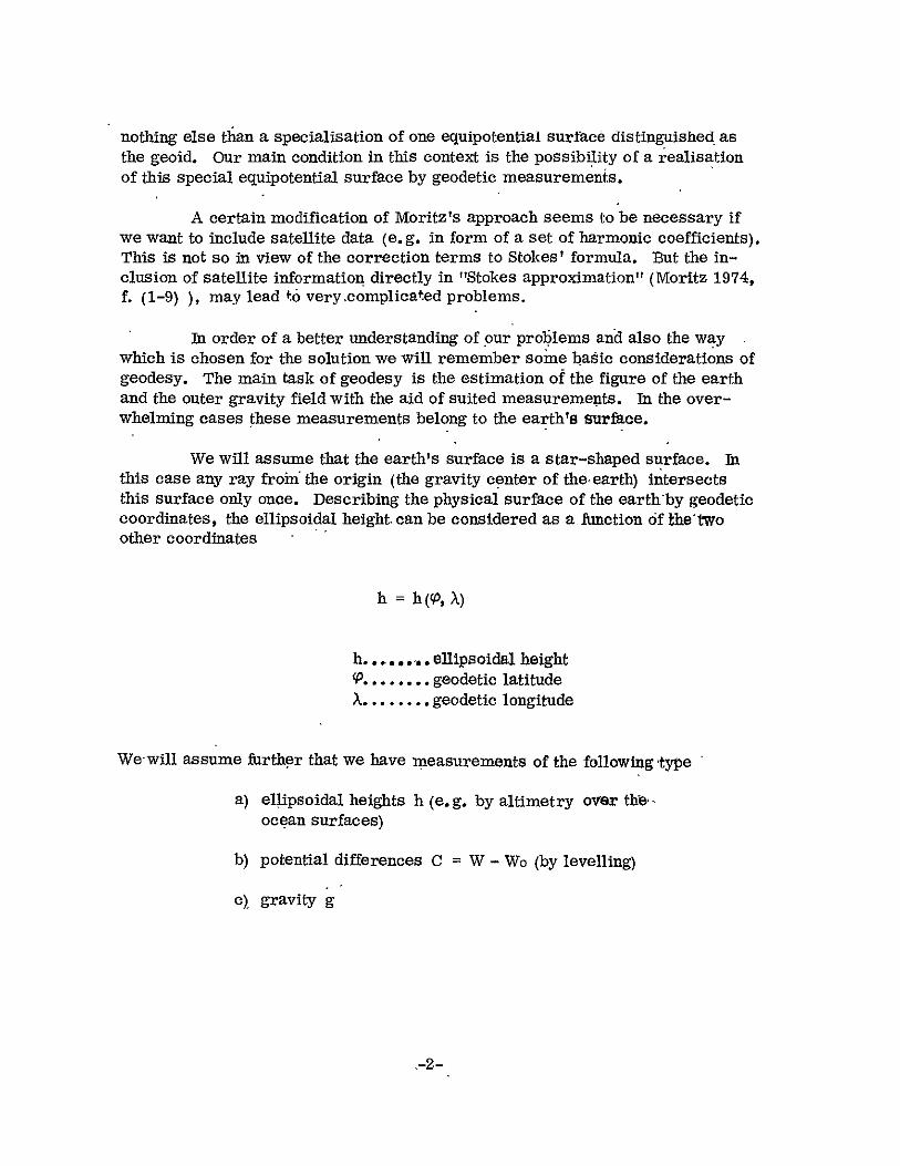
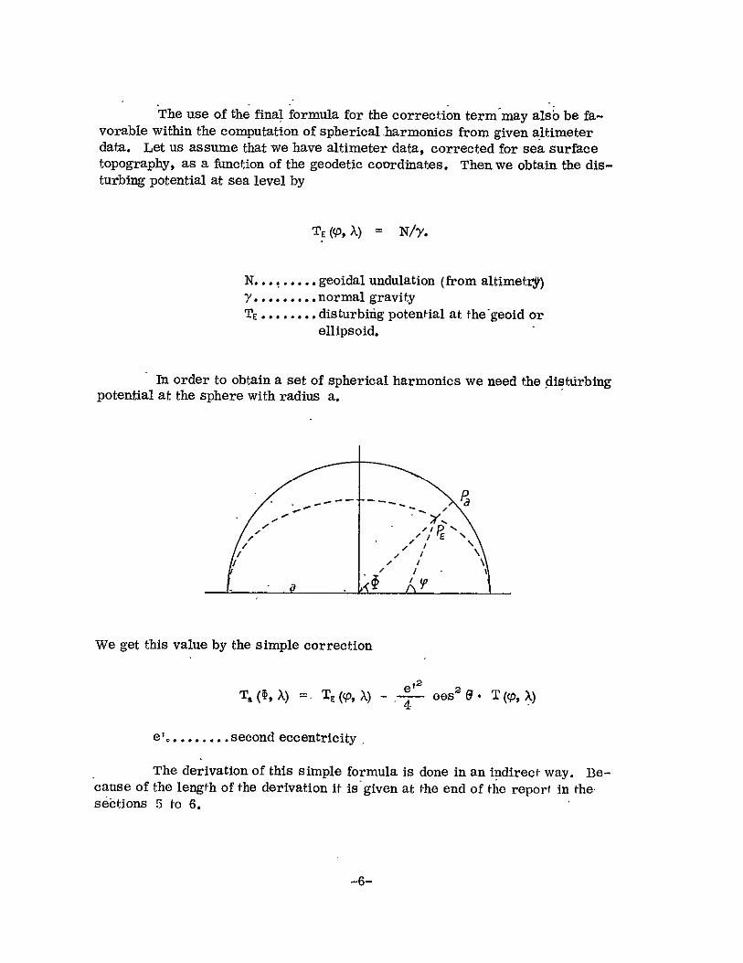
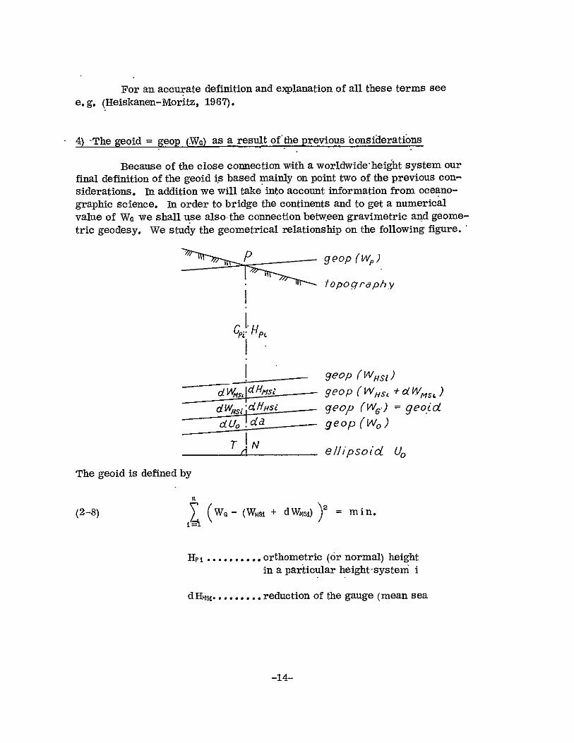
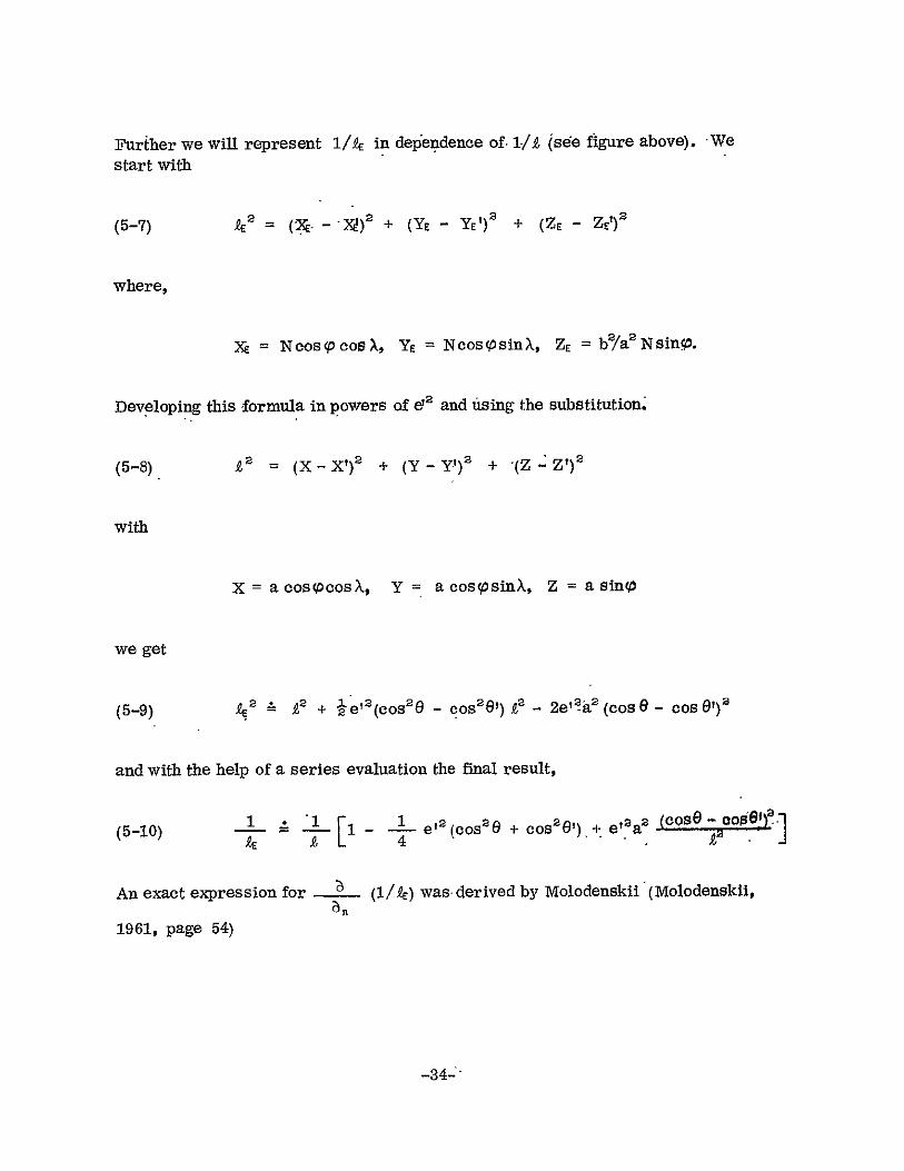

and
(6-17) r f f2 dE = a f x (I 4e2 cos2reg-)tcos d dXe
2 into a power series of the small parameter eEvaluating also T
T = Tb + e + Te
and inserting this expression in (6-17) we obtain
deg (6-18) o = fax do
and
-- Cos2regX do + af -shy(6-19) T =-aS
We get as an intermediate solution
(6-20) o a I 6nO n+ I
or written as an integral equation
(6-21) 2iro +i fT Oo = a f 6g dco
and afterwards
-45shy
n
= (2n= O (n+1)n+ 3) T(2(n X)
(6-22) i~ o
(3nplusmn+1) n
Aum Q R(n+)m(reg X-
4 n=O M-0 (n + 3)
+ B- Rnm(0X) + Y X(n + 1) ( -
Whereas usually the integrations over the unit sphere are madewith the aid of
the geodetic latitude 0 the geocentric latitudes are used as parameters in
equation (6-21) Applying here (Lelgemann 1970)
(6-23) cos - (1 + e 2 sin2 p) coso
(6-24) d ( - e 2 + 2e 2 sin2 ) dp
211 1
_______ 2sinou22sinT2 - L 2
(6-25)
os e - cos )2
e2(cos cos 2 q 44sin 22 6 + 6)
with
B = 90o-c
cosT = cos cosv + sin sinVcosAX
cos = cos pcos p + sinsinWp cos AX
-46shy
we arrive at the following integral equation system
o +I To da a 6g doTdeg + I- d = Coofa
a a
r 0A
11+~~~~~(coP - cos -iosG+cs 2
(6-26) + +-- 1 (COSin- Cos 6g Cos20 4am2 2nj
da4-cose42 e + (Cos -Cos+ sine 02 )0
T2
with
dc = sinG dO dX
We have in spherical approximation
2a6g X (2n+2) T
and therefore
(6-27) T+ 1 4Tf T- jo 4T71 (9n+ )1 a3 n=Oa
-47shy
2 2 ) 2 -Icos e + -- cos + (cOS - cos I d
-2 COSr + 4 sin 02 2
A series evaluation gives
T= 2m T + (2n +1) (4m 2 - 1) Tu TL (n + 1 T n = L (n+1)(2n+ 3)(2n-1)
(6-28) + Anm n2n cYmR(n+2m(0 ) + 2n + 1 B3rjRnm(0s X)+n+32n +2 +
+ n YnMR(n )m(X )
Adding now (6-22) and (6-28) we get
W n 2~ -n(4m 1)-
Tn + I (n+1)(2n+3)(2n-1)n---O n o m O
1 5n-1L 1rR(z+r(X)(6-29) + Anm n+3 n=O M=O
5n+ 75n+ 3+ n+ 1 nmt n-I YnrmR( ) m(0 X)fR( X)
We sum up the result by
-48shy
6T 4 tAn [ R(n+ M ( X-) + inmR (6 X) n=o m0O
+ rR(n)m(6 X)1 + Bnt[ TnS()(X) + nmSnm(6X)
+ s(S)M(6 X)]
with
- (5n-1)(n-m+1)(n-m+2) (n+ 3)(2n+ 1)(2n +3)
6m 2 + n +36 3 - amp + 6nm2 shy- 6-On(n +1)(2n+3) (2n- 1)
= (5n + 7) (n + m) (n + m -1) (n - 1)(2n + 1) (2n - 1)
In the case of the disturbing potential of the earth we have
A0o = A1 0 = Al 1 = Bil = 0
We get a proper expression of the final result from the splution of (6-21) together with a simple renumbering of the terms of this series
2(6-30) T = T + e T
(6-31) T(6 ) = a - 4 1 6g(6 X)-n4 +
-49 shy
co n
(6-32)Tn(632) = I I ECmRQX + VSn(6Xf
n~e m0o
cu = [ A(n)pn + AnmQ m + A(n-z)mrn]
=[ B(rr-)mpnh + Bnqnm + B n-)mrn]
with
(sn - 11) (n - m - 1) (n - m) Pm = 4(n+1)(2n-3)(2n-1)
-6n 3 - 8n 2 1- 6nm - 6m 2 + n 1 3
4(n + 1) (2n- 1) (2n + 3)
r (5n +17) (n + m +2) (n + m + 1)4(n + 1) (2n + 5) (2n + 3)
It may be pointed out that the gravity disturbances belong to points PE (P0 X) on the ellipsoid and the disturbing potential to points P ( X) on the sphere
-50shy
Based on this result we will derive some other useful formulae We begin with a direct relation between the gravity disturbances at the ellipsoid 6gE and the gravity disturbances 6g at the tangent sphere
(6-33) 6g = 6gE- 6f3
We use the abbreviation (q3) because the abbreviation (6g3 ) is already reserved for the gravity anomalies (see formula (4-6) ) The potential T is given on a sphere So we have the exact series relation
(6-34) ampg - a I (n + 1) (T) n =O
Inserting (6-30) into (6-34) we get as the desired result
)Rln( +S ( e(6- 35) 6 g = 6gE + 2( + t [C
) +Jenmflva tI( 1)m ~ 8 An X)n=O0
or
6g ea L~ nplusmn1 )+]~Sn(b) A) ]~m~m6 n=O m=0
Next we will derive a direct relation between the disturbing potential T at the tangent sphere and the disturbing potential TE at the ellipsoid This derivation should be performed in three steps First we compute 6g from T with the help of (6-20) Second we compute the gravity disturbances at the ellipsoid with (6-33) using for more convenience the intermediate relation (6-29) Third we compute the disturbing potential TE at the ellipsoid with formulae (5-19) and (5-31) of the previous section We arrive with the simple result
(6-36) TE = T + 6t 3
-51shy
with
6t3 = 747 f A O~(T(A + ~ X n=2 m=O
+ YR( z2)(G X) ] + B [ S(rt)m(6 X)
+ mR=(0 X) + YR(t)m(6 A) 1 3
or with the aid of (8-5)
(6-37) 6f3 - Cos 2 6Th( X)4
Because 6t3 is a term of second orderwe can neglect the difference between 6 and 9 writing also
3 4f cos 2 T(OX)
Finally we shall derive the relation between the gravity anomalies Ag at the tangent sphere and the gravity anomalies AgE at the ellipsoid sfarting from the known relation af the ellipsoid (Lelgemann 1970)
=(6-38) AgE 6g + Tl aTE - e 2 cos 2 V an a
We have by definition
(6-39) Ag = AgE - 693
-52shy
and
(6-40) Ag= 2 T a
After some manipulation we get from these formulai
6g3 = 2-(1 + e - e 2 cos 2 TE + zT
a
or as a final result
(6-41) 6g 6 - - -- cos2 e) T (6
a
67g3 (2a
It is very easy to derive (4-16) (4-17) (4-18) and (4-19) from (6-33) (6-35) and (6-41)
-53shy
7 Summary
The definition of the geoid is discussed in the first part of the present
study Of course the geoid is a certain equipotenfial surface of theearth grashy
vity field The discussion is only concerned with a specification of this equiposhy
tential surface The final proposition for a definition is based on the geodetic
height systems by an inclusion of given information from oceanographic science
about sea surface topography
First theThe realisation of the geoid should be made in two steps
existing height systems are corrected by information about sea surface toposhy
graphy An equipotential surface is choosen in such a manner that the sum of
the squares of the deviations to the corrected main height systems is a mini-
mum This particular equipotential surface is called the geoid
A least squares procedure is derived for a realisation of this definition
The precise cartesian coordinates of geophysical stations and in addition the
quasi geoidal undulations and the normal heights in these points are needed as
data The unknown corrections to the various height datums influence of course
the gravity anomalies and consequently fhe geoidal undulations This influence
is regarded in the least squares procedure
In the second part of the study a solution of Stokes problem with an acshy
curacy of bettei than plusmn10 cm is suggested in which the results of satellite geodesy
can be-included in a rather simple way The method is based on the possibility that
the potential outside the earth surface can be approximated by the potential of anashy
lytical continuation inside the earth with any accuracy Gravity anomalies from the
earths surface are reduced by three successive corrections to gravity anomalies at
the sphere with radius a At this sphere they can be combined with given potential coefficients from satellite geodesy Then the potential at the surface of the earth is computed with the aid of additional three corrections
Of special interest could be the very simple formula which connects the potential at the ellipsoid with the potential at the sphere with radius a In the computation of potential coefficients from altimeter data the influence of ellipticity can easily be taken into account with this formula
-54shy
8 Appendix
We shall derive in the appendix an evaluation of the function
(8-1) (Cos 0 -0Cos 6) 2
8 sin 2
polar distance
spherical distance between two points P and P
in a series of sphericalharmonics starting with the derivation of two formulae which we shall need in the final evaluation
As the immediate result of the kernel of Poissons integral formula (Heiskanen-Moritz 1967)
R (r-n+1
(ir2z-plusmnn+1) --a Po(COS n=o
we get for r = R
=(8-2) 7 (2n+1I)P(cosO) 0 n=O
Now we will try to deriveia series evaluation for
t 8 sin 2
In this case we do not get a well defined expression due to the relation of (8-2) The evaluation can be started with the -well known formila
-55shy
oR- Po (COScent L r ME-- = [(r-R)+4rRin2 02] 2
n=0
The fitsfderivative gives
F3 (n + 1) R 2 P (cos )
- T- [(r-R) + 2Rsin2 42]
The second derivative gives the result
2 W) - (n + 1) (n + 2) Rn P (cos ) n+3r = -r
1 1
- - +3 [(r-R) + 2Rsin2 2] 2
On the sphere with the radis R we have
0= 2Rsin42
For points on this sphere we can write
S(n + 1) (n + 2) P(Cos i)
1 3 8R 3 sin02 + 8Rsin 2
-56shy
A further evaluation gives
1 _r 3 1shy- 4 sSsin 3 2 i (n+1)(n+2) P(cos)
1=0
or
sin _ = [ (n +)(n + 2)-- P(cos8Ssin 02 pound4
n=0
With the identity
-(n +1)(n + 2) - 4 -= 4 (2n+1)(2n+5)
we get
Ssin3 4i2 - ~ (2n + 1) ( 2n + 5) P(cos 0) n=0
Because of (8-2) we can see that the evaluation of 1 info a series of spherical harmonics gives not a well defined result but an expression of the form
(83) 1 (2n +1)(n+ a) p(cos ssin3 02 n=OL 2
where a is ani given number On the other hand we shall see that in the series expression for formula (8-1) the term a drops out
-57shy
Let us start with the following expression for a fixed point P (Heiskanen-Moritz 1967)
f8(0 X) Cos Cos Oltan( V)R(O A)-
n=O M-=O
+ b(O SI( X))]
Then we can estimate the coefficients a by
a 2n +1 (n - m) ft (Cos -cos 6) 2 bull 2TT- (n+m)
(2n + 1) (n +a) P (Co ) Rnm(QX) dd
n=O2
Using twice the recursion formula for Legendre functions
cosa Pnm(cos0) n - m + 1 R( +1)m(cos0) + n + m p_ (cosG)2n + 1 2n +1
and multiplying the result with cos (mA) we get the following two expressions
(8-4) CoS Rnr(eX) - n-m+1 n+ mf (p X) + o bull 2n+1 R(n~i~m(6A) 2n+1i (n$
and
(8-5) cos 2 e Rn(O X) = mR(n+)m( 6 A)+ RnmRn( 6A)+ V11R(-)m( 6 X)
-58-
with
O 1 = (n-m-f-)(n-m-n-2) (2n + 1) (2h + 3)
2n - 2m2 + 2n - 1 (2n + 3) (2n - 1)
-= (n+ m)(n+m-1) (2n +1) (2n- 1)
With the help of this recursion formula we get due to the orthogonality relation q of spherical harmonics after the integration
an( X) (n - m) [ -(2n + 1)(n + a + 2)an (0(n + m) [
- (2n + 1) (n i-a) 1nlRn (6 X)
-(2n + 1)(n+ a -2) yR(-)1 (O X)
+ 2cos 0(n- m + 1)(n+ a + 1)R(wn)m( 6 )
+ 2cos O(n +m) (n+ -I) R(0 (O )
- cosG(2n+l)(n +a)Rnm( X)
Using the recursion formula once more the term a drops out and we are left with the result
2 (n-i) (n-m+1)(n+m+1) - (n+m)(n-m) S (n + m) [ (2n -f 3) (2n - 1)
Rn( X)
-59shy
or
4m2 - 1 = 2 (n- m)
(n + m) I (2n + 3) (2n - 1) 1146 X)
Analogous evaluations give
b =2 (n-) 4m - I S(() X) (n + m) I (2n + 3) (2n - 1)
As a final result we get the desired expression
(8-6) (cos G- cos6) 2 8 sin3 02
n= - (2n +3)(2n-) n
2 1(2n-1) P( cosO) P(cos 6)
+ 2 (n-m)1 4m 2 - R Rnm(6 XR(e) =I (n + M) (2n+ 3) (2n- 1)
+ S n( X) S n(6 X) I
-60shy
9 References
AGU (1974) The Geoid and Ocean Surface Report on the Fourth Geop Research Conference EOS Trans AGU 55 128
Gotthardt E (1968) Einfihrung in die Ausgleichungsreohnung Wichmanni Karlsruhe
Heiskanen W A and Moritz H (1967) Physical Geodesy W H Freeman San Francisco
IAG (1971) Geodetic Reference System 1967 Publication speciale du Bulletin Geodesique Paris
Koch K R and Pope A J (1972) Uniqueness and Existence for the Geodet Boundary Value Problem Using the Known Surface of the Earth Bull Geod no 106 p- 4 67
Krarup T (1969) A Contribution to the Mathematical Foundation of Physical Geodesy Pubi No 44 Danish Geodetic Institute Copenhagen
Lambert W D and Darling F W (1936) Tables for Determining the Forn of the Geoid and Its Indirect Effect on Gravity U S Coast and Geodetic Survey Spec Publ No 199
Lelgemann D (1972) Spherical Approximation and the Combination of Gravishymetric and Satellite Data Paper presented at the 5th Symposium on Mathematical Geodesy Firence Okt 1972
Lelgemann D (1970) Untersuchungen zu einer genaueren Lsung des Problems von Stokes Publ No C155 German Geodetic Commission
Mather R S (1973) A Solution of the Geodetic Boundary Value Problem t o Order e 3 Report X-592-73-11 Goddard Space flight Center
Mather B S (1974a) Geoid Definitions for the Study of SeaSurfaee Topography from Satellite Altimetry Paper presented at the Symposium on Applications of Marine Geodesy June 1974 Columbus Ohio
Mather R S (1974b) On the Evaluation of Stationary Sea Surface Topography Using Geodetic Techniques Submitted to Bulletin Geodesique
-61shy
Meissl P (1971) On the Linearisation of the Geodetic Boundary Value Proshyblem Report No 152 Department of Geodetic Science Ohio State University Columbus
Molodenskii M S Eremeev V F and Yurkina M I (1962) Methods for Study of the External Gravitational Field and Figure of the Earth Translated from Russian (1960) Israel Program for Scientific Translation Jerusalem
M6ritz H (1974) Precise Gravimetric Geodesy Report No 219 Department of Geodetic Science Ohio State Universily Columbus Ohio
Moritz H (1971) Series Solutions of Molodenskiis Problem Pubi No A70 German Geodetic Commission
Mueller I I (1974) Global Satellite Triangulation and Trilateration Results J Geophys Res 79 No 35 p 5333
Rapp R H (1973) Accuracy of Geoid Undulation Computations J Geophys Res 78 No 32 p 7589
Rapp R H (1974) The Geoid Definition and Determination EOS Trans AGU 55 118
Vincent S and Marsh J (1973) Global Detailed Gravimetric Geoid Paper presented at Ist Internaional Symposium on Use of Artificial Satellites for Geodesy and Geodynamics Athens May 14-21
Wemelsfelder P J (1970) Sea Level Observations as a Fact and as an illusion Report on the Symposium on Coastal Geodesy edited by R Sigl p 65 Institute for Astronomical and Physical Geodesy Technical University Munich
-62shy
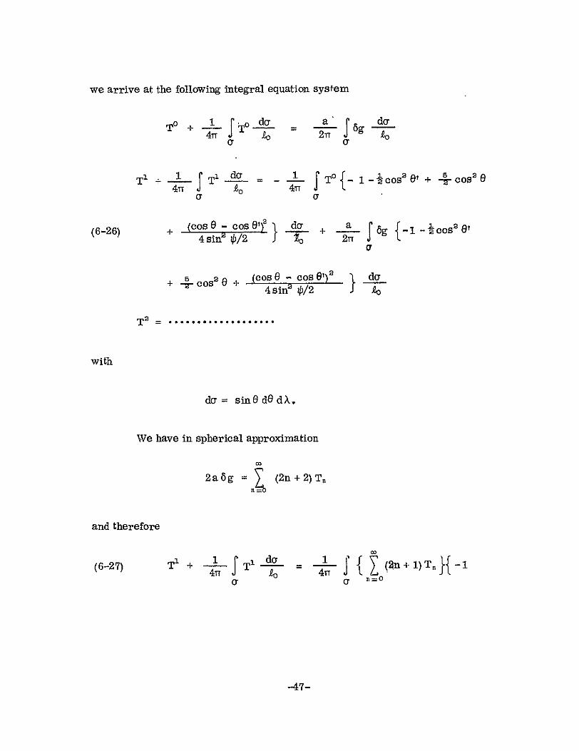
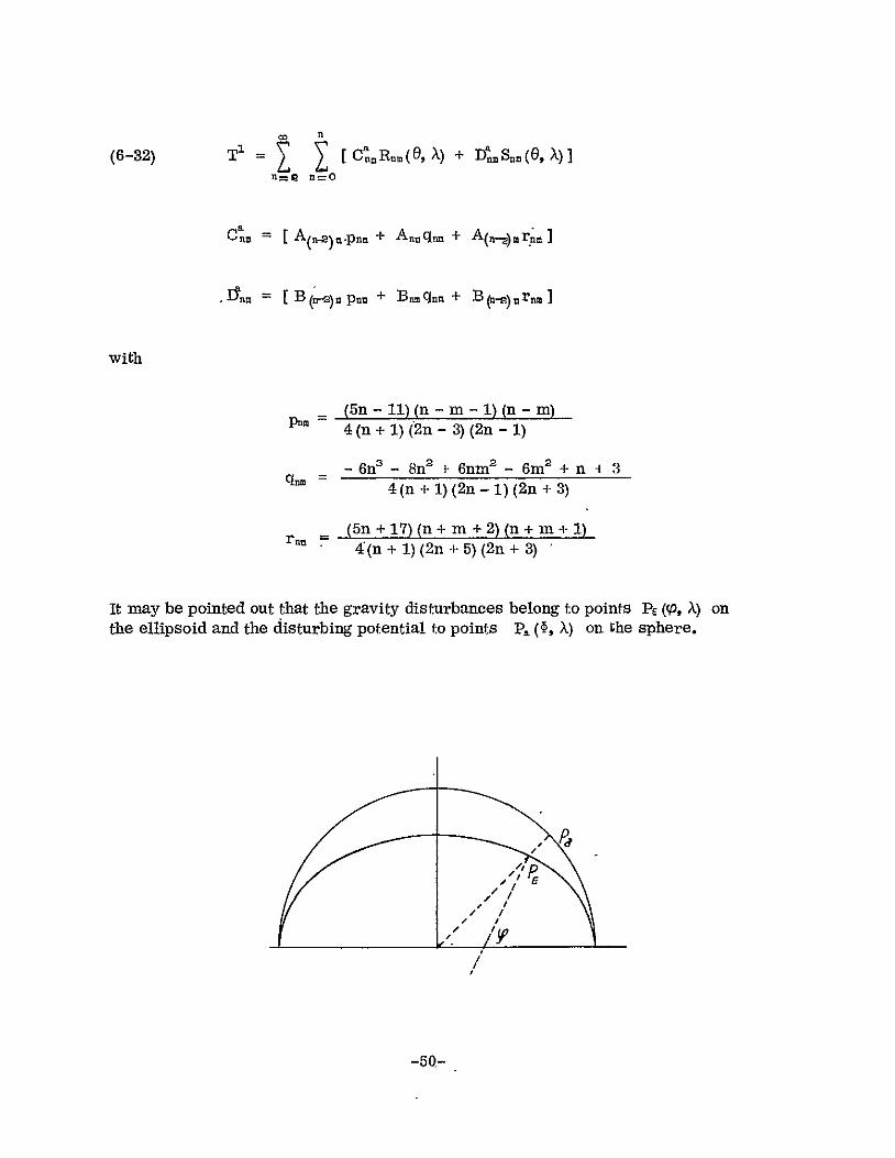

with
6t3 = 747 f A O~(T(A + ~ X n=2 m=O
+ YR( z2)(G X) ] + B [ S(rt)m(6 X)
+ mR=(0 X) + YR(t)m(6 A) 1 3
or with the aid of (8-5)
(6-37) 6f3 - Cos 2 6Th( X)4
Because 6t3 is a term of second orderwe can neglect the difference between 6 and 9 writing also
3 4f cos 2 T(OX)
Finally we shall derive the relation between the gravity anomalies Ag at the tangent sphere and the gravity anomalies AgE at the ellipsoid sfarting from the known relation af the ellipsoid (Lelgemann 1970)
=(6-38) AgE 6g + Tl aTE - e 2 cos 2 V an a
We have by definition
(6-39) Ag = AgE - 693
-52shy
and
(6-40) Ag= 2 T a
After some manipulation we get from these formulai
6g3 = 2-(1 + e - e 2 cos 2 TE + zT
a
or as a final result
(6-41) 6g 6 - - -- cos2 e) T (6
a
67g3 (2a
It is very easy to derive (4-16) (4-17) (4-18) and (4-19) from (6-33) (6-35) and (6-41)
-53shy
7 Summary
The definition of the geoid is discussed in the first part of the present
study Of course the geoid is a certain equipotenfial surface of theearth grashy
vity field The discussion is only concerned with a specification of this equiposhy
tential surface The final proposition for a definition is based on the geodetic
height systems by an inclusion of given information from oceanographic science
about sea surface topography
First theThe realisation of the geoid should be made in two steps
existing height systems are corrected by information about sea surface toposhy
graphy An equipotential surface is choosen in such a manner that the sum of
the squares of the deviations to the corrected main height systems is a mini-
mum This particular equipotential surface is called the geoid
A least squares procedure is derived for a realisation of this definition
The precise cartesian coordinates of geophysical stations and in addition the
quasi geoidal undulations and the normal heights in these points are needed as
data The unknown corrections to the various height datums influence of course
the gravity anomalies and consequently fhe geoidal undulations This influence
is regarded in the least squares procedure
In the second part of the study a solution of Stokes problem with an acshy
curacy of bettei than plusmn10 cm is suggested in which the results of satellite geodesy
can be-included in a rather simple way The method is based on the possibility that
the potential outside the earth surface can be approximated by the potential of anashy
lytical continuation inside the earth with any accuracy Gravity anomalies from the
earths surface are reduced by three successive corrections to gravity anomalies at
the sphere with radius a At this sphere they can be combined with given potential coefficients from satellite geodesy Then the potential at the surface of the earth is computed with the aid of additional three corrections
Of special interest could be the very simple formula which connects the potential at the ellipsoid with the potential at the sphere with radius a In the computation of potential coefficients from altimeter data the influence of ellipticity can easily be taken into account with this formula
-54shy
8 Appendix
We shall derive in the appendix an evaluation of the function
(8-1) (Cos 0 -0Cos 6) 2
8 sin 2
polar distance
spherical distance between two points P and P
in a series of sphericalharmonics starting with the derivation of two formulae which we shall need in the final evaluation
As the immediate result of the kernel of Poissons integral formula (Heiskanen-Moritz 1967)
R (r-n+1
(ir2z-plusmnn+1) --a Po(COS n=o
we get for r = R
=(8-2) 7 (2n+1I)P(cosO) 0 n=O
Now we will try to deriveia series evaluation for
t 8 sin 2
In this case we do not get a well defined expression due to the relation of (8-2) The evaluation can be started with the -well known formila
-55shy
oR- Po (COScent L r ME-- = [(r-R)+4rRin2 02] 2
n=0
The fitsfderivative gives
F3 (n + 1) R 2 P (cos )
- T- [(r-R) + 2Rsin2 42]
The second derivative gives the result
2 W) - (n + 1) (n + 2) Rn P (cos ) n+3r = -r
1 1
- - +3 [(r-R) + 2Rsin2 2] 2
On the sphere with the radis R we have
0= 2Rsin42
For points on this sphere we can write
S(n + 1) (n + 2) P(Cos i)
1 3 8R 3 sin02 + 8Rsin 2
-56shy
A further evaluation gives
1 _r 3 1shy- 4 sSsin 3 2 i (n+1)(n+2) P(cos)
1=0
or
sin _ = [ (n +)(n + 2)-- P(cos8Ssin 02 pound4
n=0
With the identity
-(n +1)(n + 2) - 4 -= 4 (2n+1)(2n+5)
we get
Ssin3 4i2 - ~ (2n + 1) ( 2n + 5) P(cos 0) n=0
Because of (8-2) we can see that the evaluation of 1 info a series of spherical harmonics gives not a well defined result but an expression of the form
(83) 1 (2n +1)(n+ a) p(cos ssin3 02 n=OL 2
where a is ani given number On the other hand we shall see that in the series expression for formula (8-1) the term a drops out
-57shy
Let us start with the following expression for a fixed point P (Heiskanen-Moritz 1967)
f8(0 X) Cos Cos Oltan( V)R(O A)-
n=O M-=O
+ b(O SI( X))]
Then we can estimate the coefficients a by
a 2n +1 (n - m) ft (Cos -cos 6) 2 bull 2TT- (n+m)
(2n + 1) (n +a) P (Co ) Rnm(QX) dd
n=O2
Using twice the recursion formula for Legendre functions
cosa Pnm(cos0) n - m + 1 R( +1)m(cos0) + n + m p_ (cosG)2n + 1 2n +1
and multiplying the result with cos (mA) we get the following two expressions
(8-4) CoS Rnr(eX) - n-m+1 n+ mf (p X) + o bull 2n+1 R(n~i~m(6A) 2n+1i (n$
and
(8-5) cos 2 e Rn(O X) = mR(n+)m( 6 A)+ RnmRn( 6A)+ V11R(-)m( 6 X)
-58-
with
O 1 = (n-m-f-)(n-m-n-2) (2n + 1) (2h + 3)
2n - 2m2 + 2n - 1 (2n + 3) (2n - 1)
-= (n+ m)(n+m-1) (2n +1) (2n- 1)
With the help of this recursion formula we get due to the orthogonality relation q of spherical harmonics after the integration
an( X) (n - m) [ -(2n + 1)(n + a + 2)an (0(n + m) [
- (2n + 1) (n i-a) 1nlRn (6 X)
-(2n + 1)(n+ a -2) yR(-)1 (O X)
+ 2cos 0(n- m + 1)(n+ a + 1)R(wn)m( 6 )
+ 2cos O(n +m) (n+ -I) R(0 (O )
- cosG(2n+l)(n +a)Rnm( X)
Using the recursion formula once more the term a drops out and we are left with the result
2 (n-i) (n-m+1)(n+m+1) - (n+m)(n-m) S (n + m) [ (2n -f 3) (2n - 1)
Rn( X)
-59shy
or
4m2 - 1 = 2 (n- m)
(n + m) I (2n + 3) (2n - 1) 1146 X)
Analogous evaluations give
b =2 (n-) 4m - I S(() X) (n + m) I (2n + 3) (2n - 1)
As a final result we get the desired expression
(8-6) (cos G- cos6) 2 8 sin3 02
n= - (2n +3)(2n-) n
2 1(2n-1) P( cosO) P(cos 6)
+ 2 (n-m)1 4m 2 - R Rnm(6 XR(e) =I (n + M) (2n+ 3) (2n- 1)
+ S n( X) S n(6 X) I
-60shy
9 References
AGU (1974) The Geoid and Ocean Surface Report on the Fourth Geop Research Conference EOS Trans AGU 55 128
Gotthardt E (1968) Einfihrung in die Ausgleichungsreohnung Wichmanni Karlsruhe
Heiskanen W A and Moritz H (1967) Physical Geodesy W H Freeman San Francisco
IAG (1971) Geodetic Reference System 1967 Publication speciale du Bulletin Geodesique Paris
Koch K R and Pope A J (1972) Uniqueness and Existence for the Geodet Boundary Value Problem Using the Known Surface of the Earth Bull Geod no 106 p- 4 67
Krarup T (1969) A Contribution to the Mathematical Foundation of Physical Geodesy Pubi No 44 Danish Geodetic Institute Copenhagen
Lambert W D and Darling F W (1936) Tables for Determining the Forn of the Geoid and Its Indirect Effect on Gravity U S Coast and Geodetic Survey Spec Publ No 199
Lelgemann D (1972) Spherical Approximation and the Combination of Gravishymetric and Satellite Data Paper presented at the 5th Symposium on Mathematical Geodesy Firence Okt 1972
Lelgemann D (1970) Untersuchungen zu einer genaueren Lsung des Problems von Stokes Publ No C155 German Geodetic Commission
Mather R S (1973) A Solution of the Geodetic Boundary Value Problem t o Order e 3 Report X-592-73-11 Goddard Space flight Center
Mather B S (1974a) Geoid Definitions for the Study of SeaSurfaee Topography from Satellite Altimetry Paper presented at the Symposium on Applications of Marine Geodesy June 1974 Columbus Ohio
Mather R S (1974b) On the Evaluation of Stationary Sea Surface Topography Using Geodetic Techniques Submitted to Bulletin Geodesique
-61shy
Meissl P (1971) On the Linearisation of the Geodetic Boundary Value Proshyblem Report No 152 Department of Geodetic Science Ohio State University Columbus
Molodenskii M S Eremeev V F and Yurkina M I (1962) Methods for Study of the External Gravitational Field and Figure of the Earth Translated from Russian (1960) Israel Program for Scientific Translation Jerusalem
M6ritz H (1974) Precise Gravimetric Geodesy Report No 219 Department of Geodetic Science Ohio State Universily Columbus Ohio
Moritz H (1971) Series Solutions of Molodenskiis Problem Pubi No A70 German Geodetic Commission
Mueller I I (1974) Global Satellite Triangulation and Trilateration Results J Geophys Res 79 No 35 p 5333
Rapp R H (1973) Accuracy of Geoid Undulation Computations J Geophys Res 78 No 32 p 7589
Rapp R H (1974) The Geoid Definition and Determination EOS Trans AGU 55 118
Vincent S and Marsh J (1973) Global Detailed Gravimetric Geoid Paper presented at Ist Internaional Symposium on Use of Artificial Satellites for Geodesy and Geodynamics Athens May 14-21
Wemelsfelder P J (1970) Sea Level Observations as a Fact and as an illusion Report on the Symposium on Coastal Geodesy edited by R Sigl p 65 Institute for Astronomical and Physical Geodesy Technical University Munich
-62shy

and
(6-40) Ag= 2 T a
After some manipulation we get from these formulai
6g3 = 2-(1 + e - e 2 cos 2 TE + zT
a
or as a final result
(6-41) 6g 6 - - -- cos2 e) T (6
a
67g3 (2a
It is very easy to derive (4-16) (4-17) (4-18) and (4-19) from (6-33) (6-35) and (6-41)
-53shy
7 Summary
The definition of the geoid is discussed in the first part of the present
study Of course the geoid is a certain equipotenfial surface of theearth grashy
vity field The discussion is only concerned with a specification of this equiposhy
tential surface The final proposition for a definition is based on the geodetic
height systems by an inclusion of given information from oceanographic science
about sea surface topography
First theThe realisation of the geoid should be made in two steps
existing height systems are corrected by information about sea surface toposhy
graphy An equipotential surface is choosen in such a manner that the sum of
the squares of the deviations to the corrected main height systems is a mini-
mum This particular equipotential surface is called the geoid
A least squares procedure is derived for a realisation of this definition
The precise cartesian coordinates of geophysical stations and in addition the
quasi geoidal undulations and the normal heights in these points are needed as
data The unknown corrections to the various height datums influence of course
the gravity anomalies and consequently fhe geoidal undulations This influence
is regarded in the least squares procedure
In the second part of the study a solution of Stokes problem with an acshy
curacy of bettei than plusmn10 cm is suggested in which the results of satellite geodesy
can be-included in a rather simple way The method is based on the possibility that
the potential outside the earth surface can be approximated by the potential of anashy
lytical continuation inside the earth with any accuracy Gravity anomalies from the
earths surface are reduced by three successive corrections to gravity anomalies at
the sphere with radius a At this sphere they can be combined with given potential coefficients from satellite geodesy Then the potential at the surface of the earth is computed with the aid of additional three corrections
Of special interest could be the very simple formula which connects the potential at the ellipsoid with the potential at the sphere with radius a In the computation of potential coefficients from altimeter data the influence of ellipticity can easily be taken into account with this formula
-54shy
8 Appendix
We shall derive in the appendix an evaluation of the function
(8-1) (Cos 0 -0Cos 6) 2
8 sin 2
polar distance
spherical distance between two points P and P
in a series of sphericalharmonics starting with the derivation of two formulae which we shall need in the final evaluation
As the immediate result of the kernel of Poissons integral formula (Heiskanen-Moritz 1967)
R (r-n+1
(ir2z-plusmnn+1) --a Po(COS n=o
we get for r = R
=(8-2) 7 (2n+1I)P(cosO) 0 n=O
Now we will try to deriveia series evaluation for
t 8 sin 2
In this case we do not get a well defined expression due to the relation of (8-2) The evaluation can be started with the -well known formila
-55shy
oR- Po (COScent L r ME-- = [(r-R)+4rRin2 02] 2
n=0
The fitsfderivative gives
F3 (n + 1) R 2 P (cos )
- T- [(r-R) + 2Rsin2 42]
The second derivative gives the result
2 W) - (n + 1) (n + 2) Rn P (cos ) n+3r = -r
1 1
- - +3 [(r-R) + 2Rsin2 2] 2
On the sphere with the radis R we have
0= 2Rsin42
For points on this sphere we can write
S(n + 1) (n + 2) P(Cos i)
1 3 8R 3 sin02 + 8Rsin 2
-56shy
A further evaluation gives
1 _r 3 1shy- 4 sSsin 3 2 i (n+1)(n+2) P(cos)
1=0
or
sin _ = [ (n +)(n + 2)-- P(cos8Ssin 02 pound4
n=0
With the identity
-(n +1)(n + 2) - 4 -= 4 (2n+1)(2n+5)
we get
Ssin3 4i2 - ~ (2n + 1) ( 2n + 5) P(cos 0) n=0
Because of (8-2) we can see that the evaluation of 1 info a series of spherical harmonics gives not a well defined result but an expression of the form
(83) 1 (2n +1)(n+ a) p(cos ssin3 02 n=OL 2
where a is ani given number On the other hand we shall see that in the series expression for formula (8-1) the term a drops out
-57shy
Let us start with the following expression for a fixed point P (Heiskanen-Moritz 1967)
f8(0 X) Cos Cos Oltan( V)R(O A)-
n=O M-=O
+ b(O SI( X))]
Then we can estimate the coefficients a by
a 2n +1 (n - m) ft (Cos -cos 6) 2 bull 2TT- (n+m)
(2n + 1) (n +a) P (Co ) Rnm(QX) dd
n=O2
Using twice the recursion formula for Legendre functions
cosa Pnm(cos0) n - m + 1 R( +1)m(cos0) + n + m p_ (cosG)2n + 1 2n +1
and multiplying the result with cos (mA) we get the following two expressions
(8-4) CoS Rnr(eX) - n-m+1 n+ mf (p X) + o bull 2n+1 R(n~i~m(6A) 2n+1i (n$
and
(8-5) cos 2 e Rn(O X) = mR(n+)m( 6 A)+ RnmRn( 6A)+ V11R(-)m( 6 X)
-58-
with
O 1 = (n-m-f-)(n-m-n-2) (2n + 1) (2h + 3)
2n - 2m2 + 2n - 1 (2n + 3) (2n - 1)
-= (n+ m)(n+m-1) (2n +1) (2n- 1)
With the help of this recursion formula we get due to the orthogonality relation q of spherical harmonics after the integration
an( X) (n - m) [ -(2n + 1)(n + a + 2)an (0(n + m) [
- (2n + 1) (n i-a) 1nlRn (6 X)
-(2n + 1)(n+ a -2) yR(-)1 (O X)
+ 2cos 0(n- m + 1)(n+ a + 1)R(wn)m( 6 )
+ 2cos O(n +m) (n+ -I) R(0 (O )
- cosG(2n+l)(n +a)Rnm( X)
Using the recursion formula once more the term a drops out and we are left with the result
2 (n-i) (n-m+1)(n+m+1) - (n+m)(n-m) S (n + m) [ (2n -f 3) (2n - 1)
Rn( X)
-59shy
or
4m2 - 1 = 2 (n- m)
(n + m) I (2n + 3) (2n - 1) 1146 X)
Analogous evaluations give
b =2 (n-) 4m - I S(() X) (n + m) I (2n + 3) (2n - 1)
As a final result we get the desired expression
(8-6) (cos G- cos6) 2 8 sin3 02
n= - (2n +3)(2n-) n
2 1(2n-1) P( cosO) P(cos 6)
+ 2 (n-m)1 4m 2 - R Rnm(6 XR(e) =I (n + M) (2n+ 3) (2n- 1)
+ S n( X) S n(6 X) I
-60shy
9 References
AGU (1974) The Geoid and Ocean Surface Report on the Fourth Geop Research Conference EOS Trans AGU 55 128
Gotthardt E (1968) Einfihrung in die Ausgleichungsreohnung Wichmanni Karlsruhe
Heiskanen W A and Moritz H (1967) Physical Geodesy W H Freeman San Francisco
IAG (1971) Geodetic Reference System 1967 Publication speciale du Bulletin Geodesique Paris
Koch K R and Pope A J (1972) Uniqueness and Existence for the Geodet Boundary Value Problem Using the Known Surface of the Earth Bull Geod no 106 p- 4 67
Krarup T (1969) A Contribution to the Mathematical Foundation of Physical Geodesy Pubi No 44 Danish Geodetic Institute Copenhagen
Lambert W D and Darling F W (1936) Tables for Determining the Forn of the Geoid and Its Indirect Effect on Gravity U S Coast and Geodetic Survey Spec Publ No 199
Lelgemann D (1972) Spherical Approximation and the Combination of Gravishymetric and Satellite Data Paper presented at the 5th Symposium on Mathematical Geodesy Firence Okt 1972
Lelgemann D (1970) Untersuchungen zu einer genaueren Lsung des Problems von Stokes Publ No C155 German Geodetic Commission
Mather R S (1973) A Solution of the Geodetic Boundary Value Problem t o Order e 3 Report X-592-73-11 Goddard Space flight Center
Mather B S (1974a) Geoid Definitions for the Study of SeaSurfaee Topography from Satellite Altimetry Paper presented at the Symposium on Applications of Marine Geodesy June 1974 Columbus Ohio
Mather R S (1974b) On the Evaluation of Stationary Sea Surface Topography Using Geodetic Techniques Submitted to Bulletin Geodesique
-61shy
Meissl P (1971) On the Linearisation of the Geodetic Boundary Value Proshyblem Report No 152 Department of Geodetic Science Ohio State University Columbus
Molodenskii M S Eremeev V F and Yurkina M I (1962) Methods for Study of the External Gravitational Field and Figure of the Earth Translated from Russian (1960) Israel Program for Scientific Translation Jerusalem
M6ritz H (1974) Precise Gravimetric Geodesy Report No 219 Department of Geodetic Science Ohio State Universily Columbus Ohio
Moritz H (1971) Series Solutions of Molodenskiis Problem Pubi No A70 German Geodetic Commission
Mueller I I (1974) Global Satellite Triangulation and Trilateration Results J Geophys Res 79 No 35 p 5333
Rapp R H (1973) Accuracy of Geoid Undulation Computations J Geophys Res 78 No 32 p 7589
Rapp R H (1974) The Geoid Definition and Determination EOS Trans AGU 55 118
Vincent S and Marsh J (1973) Global Detailed Gravimetric Geoid Paper presented at Ist Internaional Symposium on Use of Artificial Satellites for Geodesy and Geodynamics Athens May 14-21
Wemelsfelder P J (1970) Sea Level Observations as a Fact and as an illusion Report on the Symposium on Coastal Geodesy edited by R Sigl p 65 Institute for Astronomical and Physical Geodesy Technical University Munich
-62shy
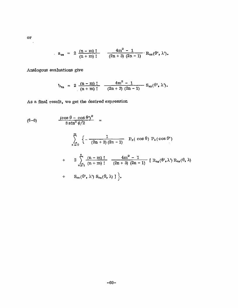