Embed Size (px)
Citation preview
SOME ASPECTS OF THE SPATIAL UNILATERAL AUTOREGRESSIVE
MOVING AVERAGE MODEL FOR REGULAR GRID DATA
By
NORHASHIDAH BINTI AWANG
Thesis Submitted to the School of Graduate Studies, Universiti Putra Malaysia,
in Fulfilment of the Requirements for the Degree of Doctor of Philosophy
February 2005

ii
To
Mother and Family
And
In the memory of a loving father,
Awang bin Ahmad (1928-1983).
May Allah rest his soul.
iii
Abstract of thesis presented to the Senate of Universiti Putra Malaysia in fulfilment
of the requirement for the degree of Doctor of Philosophy
SOME ASPECTS OF THE SPATIAL UNILATERAL AUTOREGRESSIVE
MOVING AVERAGE MODEL FOR REGULAR GRID DATA
By
NORHASHIDAH BINTI AWANG
February 2005
Chairman: Mahendran Shitan, PhD
Faculty: Science
Spatial statistics has received much attention in the last three decades and has
covered various disciplines. It involves methods which take into account the
locational information for exploring and modelling the data. Many models have
been considered for spatial processes and these include the Simultaneous
Autoregressive model, the Conditional Autoregressive model and the Moving
Average model. However, most researchers focused only on first-order models. In
this thesis, a second-order spatial unilateral Autoregressive Moving Average
(ARMA) model, denoted as ARMA(2,1;2,1) model, is introduced and some
properties of this model are studied. This model is a special case of the spatial
unilateral models which is believed to be useful in describing and modelling spatial
correlations in the data. It is also important in the field of digital filtering and
systems theory and for data whenever there is a natural ordering to the sites.
Some explicit stationarity conditions for this model are established and some
numerical computer simulations are conducted to verify the results. The general

iv
explicit correlation structure for this model over the fourth quadrant is obtained
which is then specialised to AR(2,1), MA(2,1) and the second-order separable
models. The results from simulation studies show that the theoretical correlations are
in good agreement with the empirical correlations. A procedure using the maximum
likelihood (ML) method is provided to estimate the parameters of the AR(2,1)
model. This procedure is then extended to the case of spatial AR model of any order.
For the AR(2,1) model, in terms of the absolute bias and the RMSE value, the
results from simulation studies show that this estimator outperforms the other
estimators, namely the Yule-Walker estimator, the ‘unbiased’ Yule-Walker
estimator and the conditional Least Squares estimator. The ML procedure is then
demonstrated by fitting the AR(1,1) and AR(2,1) models to two sets of data. Since
the AR(2,1) model has the second-order terms which are only in one direction, two
types of data orientation are taken into consideration. The results show that there is a
preferred orientation of these data sets and the AR(2,1) model gives better fit.
Finally, some directions for further research are given.
In this research, inter alia, the field of spatial modelling has been advanced by
establishing the explicit stationarity conditions for the ARMA(2,1;2,1) model, by
deriving the explicit correlation structure over the fourth lag quadrant for
ARMA(2,1;2,1) model and its special cases and by providing a modified practical
procedure to estimate the parameters of the spatial unilateral AR model.

v
Abstrak tesis yang dikemukakan kepada Senat Universiti Putra Malaysia sebagai
memenuhi keperluan untuk ijazah Doktor Falsafah
BEBERAPA ASPEK TENTANG MODEL RERUANG SESISI
AUTOREGRESI PURATA BERGERAK BAGI DATA GRID SEKATA
Oleh
NORHASHIDAH BINTI AWANG
Februari 2005
Pengerusi: Mahendran Shitan, PhD
Fakulti: Sains
Statistik reruang mula mendapat lebih perhatian semenjak tiga dekad lalu dan ia
mencakupi pelbagai disiplin ilmu. Statistik ini melibatkan kaedah-kaedah yang
mengambilkira maklumat lokasi dalam menjelajah dan memodel data reruang.
Banyak model yang telah dipertimbangkan bagi proses reruang termasuk model
autoregresi serentak, model autoregresi bersyarat dan model purata bergerak. Namun
demikian, hampir kesemua kajian ditumpukan pada model peringkat pertama.
Dalam tesis ini, model reruang sesisi autoregresi purata bergerak (ARMA) peringkat
kedua, ditulis sebagai ARMA(2,1;2,1) diperkenalkan dan sifat-sifatnya dikaji. Ia
adalah kes istimewa model reruang sesisi yang bermanfaat dalam menerang dan
memodel korelasi reruang yang wujud dalam data. Ia juga penting dalam ilmu
penyaringan digital dan sistem teori dan bilamana terdapat penertiban semulajadi
pada tapak data.
Beberapa syarat tak tersirat bagi kepegunan model ini diperolehi dan keputusan
disahkan dengan ujian simulasi komputer berangka. Struktur korelasi tak tersirat
vi
bagi model ini berserta kes-kes khasnya seperti model AR(2,1), model MA(2,1) dan
model-model terpisahkan peringkat kedua diperolehi bagi sukuan keempat jeda.
Keputusan ujian simulasi menunjukkan bahawa struktur korelasi yang diperolehi ini
berpadanan dengan korelasi empirik. Prosedur penganggaran menggunakan kaedah
kebolehjadian maksimum (ML) diperolehi bagi menganggar parameter model
AR(2,1). Prosedur ini kemudiannya diperluaskan kepada model reruang sesisi
autoregresi (AR) sebarang peringkat. Bagi model AR(2,1), kajian simulasi
menunjukkan kaedah ML ini adalah lebih baik secara keseluruhannya berbanding
kaedah-kaedah lain seperti Yule-Walker (YW), YW saksama dan kuasa dua terkecil
bersyarat berdasarkan nilai pincang mutlak dan punca min ralat kuasa dua. Kaedah
ML ini didemonstrasi dengan menyuai model AR(1,1) dan model AR(2,1) pada dua
set data. Memandangkan model AR(2,1) mengandungi sebutan-sebutan peringkat
kedua pada satu arah sahaja, dua jenis orientasi data dipertimbangkan. Kajian
mendapati orientasi yang berbeza memberikan keputusan yang berbeza dan secara
amnya model AR(2,1) adalah lebih baik bagi dua set data ini. Akhir sekali, beberapa
arahtuju bagi penyelidikan lanjut dicadangkan.
Dalam penyelidikan ini, ilmu permodelan reruang dimajukan antaranya dengan
menyediakan syarat-syarat kepegunan tak tersirat bagi model ARMA(2,1;2,1),
dengan menerbitkan struktur korelasi tak tersirat bagi sukuan keempat jeda untuk
model ini dan kes-kes khasnya, dan dengan menyediakan prosedur terubahsuai yang
praktikal untuk menganggar parameter model reruang sesisi AR.

vii
ACKNOWLEDGEMENTS
This thesis would not have been possible without the help and support of many
people. Firstly, I would like to express my sincerest gratitude to my advisor, Dr.
Mahendran Shitan, for his invaluable advice, patience, guidance, discussion and co-
operation during my years as a postgraduate student.
I would also like to thank the members of the supervisory committee, Associate
Professor Dr. Isa Daud and Associate Professor Dr. Mohd. Rizam Abu Bakar for
their valuable comments and being helpful during the completion of this thesis.
My special thanks and appreciation also go to all the members of Department of
Mathematics, Universiti Putra Malaysia for their kind assistance during my study.
These particularly go to the Head and former Heads of Department. To Associate
Professor Dr. Habshah Midi and Associate Professor Dr. Kassim Haron, thank you
for allowing me to attend your excellent lectures on Mathematical Statistics and
Stochastic Processes.
I am also indebted to Universiti Sains Malaysia for the scholarship awarded which
enables me to pursue my study.
I would like to convey my sincerest thanks to all my friends especially Maiyastri,
Saidatulnisa, Jayanthi and Faiz for their support and help. For those whose names

viii
were not mentioned here, the moral support and friendship they offered will be
remembered.
Lastly, my thanks also go to my family. Without their love, encouragement and
support I would not have been able to complete this work. This thesis is dedicated to
them.

ix
I certify that an Examination Committee met on 22nd February 2005 to conduct the
final examination of Norhashidah Awang on her Doctor of Philosophy thesis
entitled “Some Aspects of the Spatial Unilateral Autoregressive Moving Average
Model for Regular Grid Data” in accordance with Universiti Pertanian Malaysia
(Higher Degree) Act 1980 and Universiti Pertanian Malaysia (Higher Degree)
Regulation 1981. The Committee recommends that the candidate be awarded the
relevant degree. Members of the Examination Committee are as follows:
Habshah Midi, PhD
Associate Professor
Faculty of Science
Universiti Putra Malaysia
(Chairman)
Nor Akma Ibrahim, PhD
Associate Professor
Faculty of Science
Universiti Putra Malaysia
(Member)
Kassim Haron, PhD
Associate Professor
Faculty of Science
Universiti Putra Malaysia
(Member)
Shyamala Nagaraj, PhD Professor
Department of Applied Statistics
Faculty of Economics and Administration
Universiti Malaya
(Independent Examiner)
___________________________________
GULAM RUSUL RAHMAT ALI, PhD Professor/Deputy Dean
School of Graduate Studies
Universiti Putra Malaysia
Date:
x
This thesis submitted to the Senate of Universiti Putra Malaysia and has been
accepted as fulfilment of the requirement for the degree of Doctor of Philosophy.
The members of the Supervisory Committee are as follows:
Mahendran Shitan, PhD
Faculty of Science
Universiti Putra Malaysia
(Chairman)
Isa Daud, PhD
Associate Professor
Faculty of Science
Universiti Putra Malaysia
(Member)
Mohd. Rizam Abu Bakar, PhD
Associate Professor
Faculty of Science
Universiti Putra Malaysia
(Member)
__________________________
AINI IDERIS, PhD Professor/Dean
School of Graduate Studies
Universiti Putra Malaysia
Date:

xi
DECLARATION
I hereby declare that the thesis is based on my original work except for quotations
and citations which have been duly acknowledged. I also declare that it has not been
previously or concurrently submitted for any other degree at UPM or other
institutions.
______________________________
NORHASHIDAH BINTI AWANG
Date:
xii
TABLE OF CONTENTS
Page
DEDICATION ii
ABSTRACT iii
ABSTRAK v
ACKNOWLEDGEMENTS vii
APPROVAL ix
DECLARATION xi
LIST OF TABLES xiv
LIST OF FIGURES xvii
LIST OF ABBREVIATIONS xx
CHAPTER
1 INTRODUCTION
1.1 Introduction to Spatial Processes 2
1.2 Statement of Problems 4
1.3 Research Objectives 7
1.4 Organisation of Thesis 9
2 LITERATURE REVIEW
2.1 The Simultaneous Autoregressive (SAR) Model 11
2.2 The Conditional Autoregressive (CAR) Model 15
2.3 The Moving Average (MA) Model 16
2.4 The Spatial Autoregressive Moving Average (ARMA) Model 17
2.5 The Unilateral Model 18
2.6 The Separable (Linear-by-linear) Model 22
2.7 The First-order Spatial Unilateral ARMA Model 26
2.8 The Second-order Spatial Unilateral ARMA Model 29
3 SOME EXPLICIT STATIONARITY CONDITIONS FOR THE
SECOND-ORDER SPATIAL UNILATERAL ARMA MODEL
3.1 The Concept of Spatially Stationarity 30
3.2 Some Explicit Stationarity Conditions for the
Second-Order Spatial Unilateral ARMA Model 32
3.3 Numerical Examples 36
4 THE EXPLICIT CORRELATION STRUCTURE FOR THE
SECOND-ORDER SPATIAL UNILATERAL ARMA MODEL
OVER THE FOURTH LAG QUADRANT
4.1 Introduction 44
4.2 Stationary Representation of the Second-Order Spatial
Unilateral ARMA Model 45
4.3 The Explicit Correlation Structure for the Second-Order
Spatial Unilateral ARMA Model Over the Fourth Lag Quadrant
4.3.1 Derivation of Some Initial Terms 47
xiii
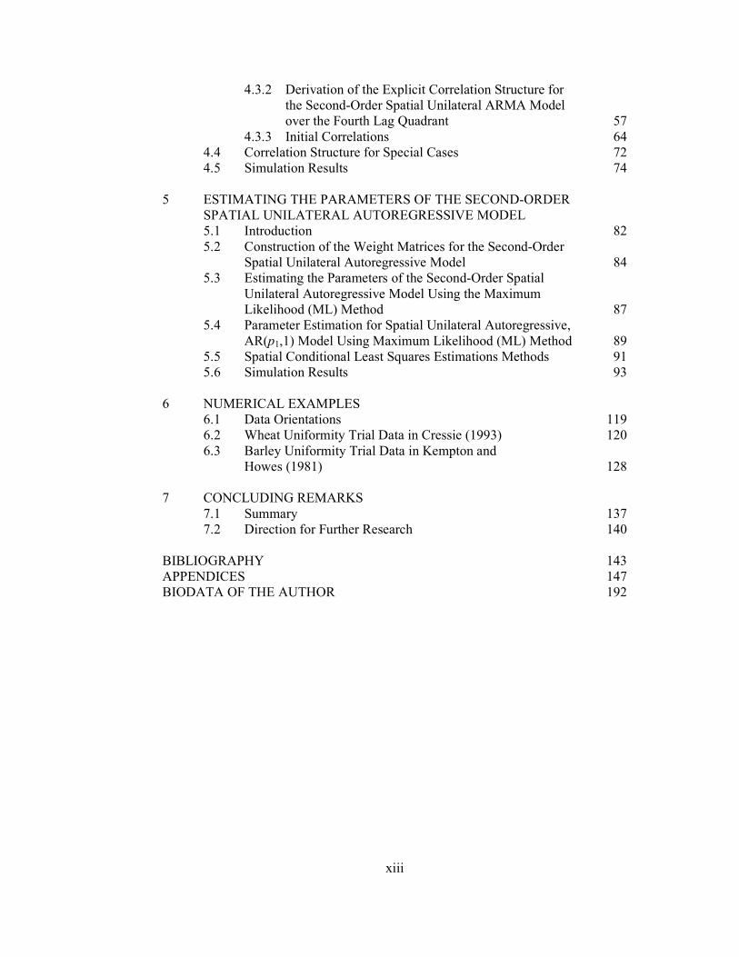
4.3.2 Derivation of the Explicit Correlation Structure for
the Second-Order Spatial Unilateral ARMA Model
over the Fourth Lag Quadrant 57
4.3.3 Initial Correlations 64
4.4 Correlation Structure for Special Cases 72
4.5 Simulation Results 74
5 ESTIMATING THE PARAMETERS OF THE SECOND-ORDER
SPATIAL UNILATERAL AUTOREGRESSIVE MODEL
5.1 Introduction 82
5.2 Construction of the Weight Matrices for the Second-Order
Spatial Unilateral Autoregressive Model 84
5.3 Estimating the Parameters of the Second-Order Spatial
Unilateral Autoregressive Model Using the Maximum
Likelihood (ML) Method 87
5.4 Parameter Estimation for Spatial Unilateral Autoregressive,
AR(p1,1) Model Using Maximum Likelihood (ML) Method 89
5.5 Spatial Conditional Least Squares Estimations Methods 91
5.6 Simulation Results 93
6 NUMERICAL EXAMPLES
6.1 Data Orientations 119
6.2 Wheat Uniformity Trial Data in Cressie (1993) 120
6.3 Barley Uniformity Trial Data in Kempton and
Howes (1981) 128
7 CONCLUDING REMARKS
7.1 Summary 137
7.2 Direction for Further Research 140
BIBLIOGRAPHY 143
APPENDICES 147
BIODATA OF THE AUTHOR 192
xiv
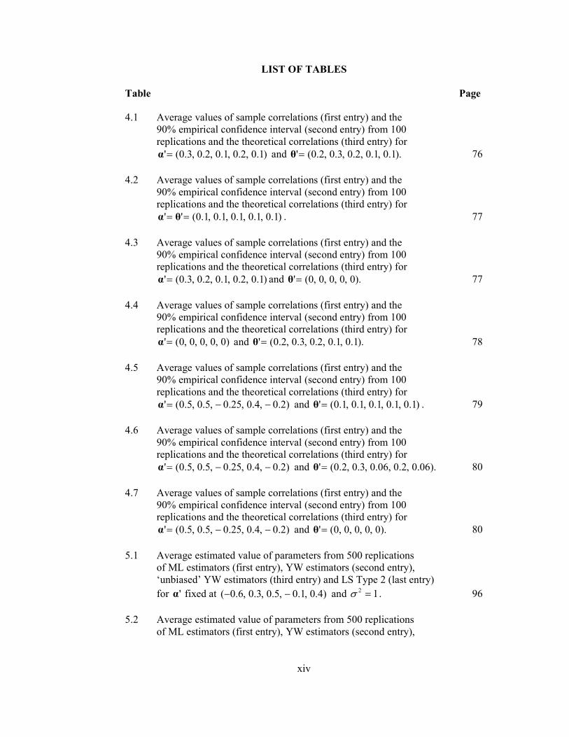
LIST OF TABLES
Table Page
4.1 Average values of sample correlations (first entry) and the
90% empirical confidence interval (second entry) from 100
replications and the theoretical correlations (third entry) for
)1.0,2.0,1.0,2.0,3.0('=α and ).1.0,1.0,2.0,3.0,2.0('=θ 76
4.2 Average values of sample correlations (first entry) and the
90% empirical confidence interval (second entry) from 100
replications and the theoretical correlations (third entry) for
)1.0,1.0,1.0,1.0,1.0('' == θα . 77
4.3 Average values of sample correlations (first entry) and the
90% empirical confidence interval (second entry) from 100
replications and the theoretical correlations (third entry) for
)1.0,2.0,1.0,2.0,3.0('=α and ).0,0,0,0,0('=θ 77
4.4 Average values of sample correlations (first entry) and the
90% empirical confidence interval (second entry) from 100
replications and the theoretical correlations (third entry) for
)0,0,0,0,0('=α and ).1.0,1.0,2.0,3.0,2.0('=θ 78
4.5 Average values of sample correlations (first entry) and the
90% empirical confidence interval (second entry) from 100
replications and the theoretical correlations (third entry) for
)2.0,4.0,25.0,5.0,5.0(' −−=α and )1.0,1.0,1.0,1.0,1.0('=θ . 79
4.6 Average values of sample correlations (first entry) and the
90% empirical confidence interval (second entry) from 100
replications and the theoretical correlations (third entry) for
)2.0,4.0,25.0,5.0,5.0(' −−=α and ).06.0,2.0,06.0,3.0,2.0('=θ 80
4.7 Average values of sample correlations (first entry) and the
90% empirical confidence interval (second entry) from 100
replications and the theoretical correlations (third entry) for
)2.0,4.0,25.0,5.0,5.0(' −−=α and ).0,0,0,0,0('=θ 80
5.1 Average estimated value of parameters from 500 replications
of ML estimators (first entry), YW estimators (second entry),
‘unbiased’ YW estimators (third entry) and LS Type 2 (last entry)
for 'α fixed at )4.0,1.0,5.0,3.0,6.0( −− and 12 =σ . 96
5.2 Average estimated value of parameters from 500 replications
of ML estimators (first entry), YW estimators (second entry),
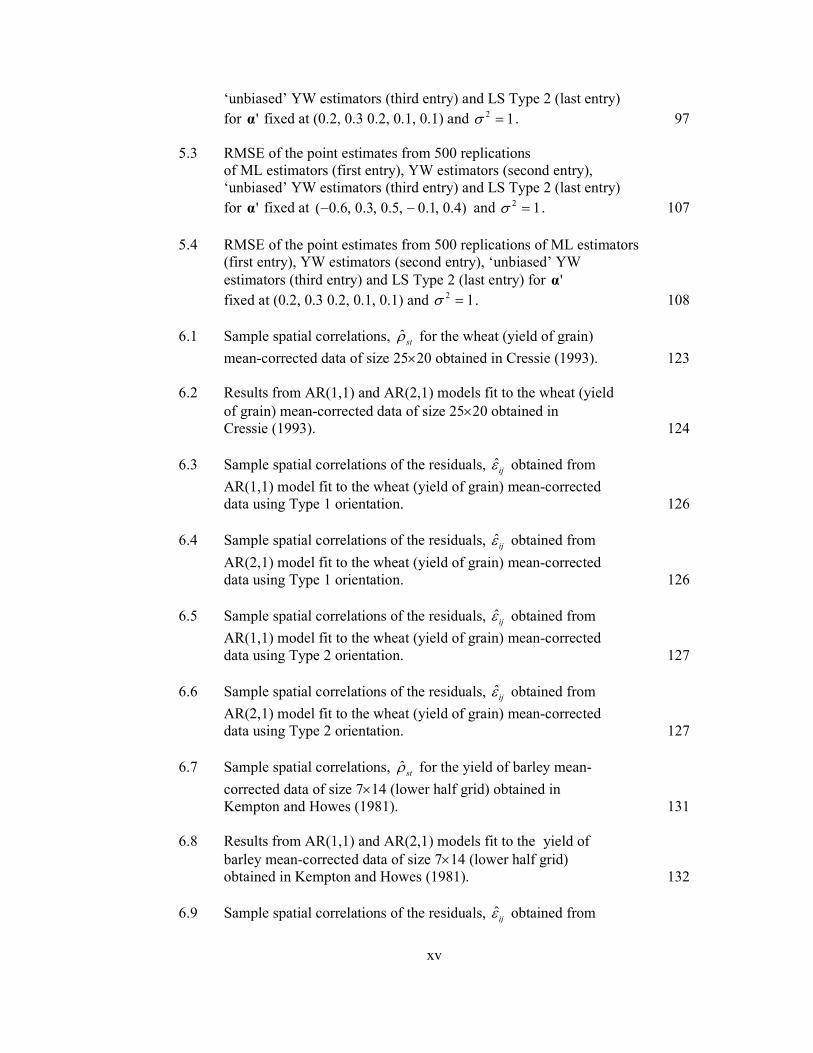
xv
‘unbiased’ YW estimators (third entry) and LS Type 2 (last entry)
for 'α fixed at (0.2, 0.3 0.2, 0.1, 0.1) and 12 =σ . 97
5.3 RMSE of the point estimates from 500 replications
of ML estimators (first entry), YW estimators (second entry),
‘unbiased’ YW estimators (third entry) and LS Type 2 (last entry)
for 'α fixed at )4.0,1.0,5.0,3.0,6.0( −− and 12 =σ . 107
5.4 RMSE of the point estimates from 500 replications of ML estimators
(first entry), YW estimators (second entry), ‘unbiased’ YW
estimators (third entry) and LS Type 2 (last entry) for 'α
fixed at (0.2, 0.3 0.2, 0.1, 0.1) and 12 =σ . 108
6.1 Sample spatial correlations, stρ for the wheat (yield of grain)
mean-corrected data of size 25×20 obtained in Cressie (1993). 123
6.2 Results from AR(1,1) and AR(2,1) models fit to the wheat (yield
of grain) mean-corrected data of size 25×20 obtained in
Cressie (1993). 124
6.3 Sample spatial correlations of the residuals, ijε obtained from
AR(1,1) model fit to the wheat (yield of grain) mean-corrected
data using Type 1 orientation. 126
6.4 Sample spatial correlations of the residuals, ijε obtained from
AR(2,1) model fit to the wheat (yield of grain) mean-corrected
data using Type 1 orientation. 126
6.5 Sample spatial correlations of the residuals, ijε obtained from
AR(1,1) model fit to the wheat (yield of grain) mean-corrected
data using Type 2 orientation. 127
6.6 Sample spatial correlations of the residuals, ijε obtained from
AR(2,1) model fit to the wheat (yield of grain) mean-corrected
data using Type 2 orientation. 127
6.7 Sample spatial correlations, stρ for the yield of barley mean-
corrected data of size 7×14 (lower half grid) obtained in
Kempton and Howes (1981). 131
6.8 Results from AR(1,1) and AR(2,1) models fit to the yield of
barley mean-corrected data of size 7×14 (lower half grid)
obtained in Kempton and Howes (1981). 132
6.9 Sample spatial correlations of the residuals, ijε obtained from
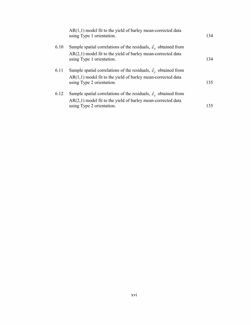
xvi
AR(1,1) model fit to the yield of barley mean-corrected data
using Type 1 orientation. 134
6.10 Sample spatial correlations of the residuals, ijε obtained from
AR(2,1) model fit to the yield of barley mean-corrected data
using Type 1 orientation. 134
6.11 Sample spatial correlations of the residuals, ijε obtained from
AR(1,1) model fit to the yield of barley mean-corrected data
using Type 2 orientation. 135
6.12 Sample spatial correlations of the residuals, ijε obtained from
AR(2,1) model fit to the yield of barley mean-corrected data
using Type 2 orientation. 135
xvii
LIST OF FIGURES
Figure Page
2.1 Quadrant Process. 19
2.2 Non-Symmetric Half Plane (NSHP) Process. 19
3.1a The generated spatial series with )1.0,2.0,1.0,2.0,3.0('=α . 36
3.1b Visualisation of the generated spatial series with )1.0,2.0,1.0,2.0,3.0('=α from different angles. 37
3.2a The generated spatial series with )2.0,2.0,2.0,0.1,2.0('=α . 38
3.2b Visualisation of the generated spatial series with
)2.0,2.0,2.0,0.1,2.0('=α from different angles. 38
3.3a The generated spatial series with )3.0,2.0,4.0,4.0,2.0(' −=α . 39
3.3b Visualisation of the generated spatial series with
)3.0,2.0,4.0,4.0,2.0(' −=α from different angles. 39
3.4a The generated spatial series with )3.0,3.0,1.0,6.0,6.0('=α . 40
3.4b Visualisation of the generated spatial series with
)3.0,3.0,1.0,6.0,6.0('=α from different angles. 40
3.5a The generated spatial series with )3.0,6.0,1.0,4.0,1.0('=α . 41
3.5b Visualisation of the generated spatial series with
)3.0,6.0,1.0,4.0,1.0('=α from different angles. 41
3.6a The generated spatial series with )32.0,4.0,56.0,8.0,7.0(' −−=α . 42
3.6b Visualisation of the generated spatial series with
)32.0,4.0,56.0,8.0,7.0(' −−=α from different angles. 42
5.1 Absolute bias of point estimates, 10α vs. grid size from 500
replications for 'α fixed at )4.0,1.0,5.0,3.0,6.0( −− . 99
5.2 Absolute bias of point estimates, 01α vs. grid size from 500
replications for 'α fixed at )4.0,1.0,5.0,3.0,6.0( −− . 100
5.3 Absolute bias of point estimates, 11α vs. grid size from 500
xviii
replications for 'α fixed at )4.0,1.0,5.0,3.0,6.0( −− . 100
5.4 Absolute bias of point estimates, 20α vs. grid size from 500
replications for 'α fixed at )4.0,1.0,5.0,3.0,6.0( −− . 101
5.5 Absolute bias of point estimates, 21α vs. grid size from 500
replications for 'α fixed at )4.0,1.0,5.0,3.0,6.0( −− . 101
5.6 Absolute bias of point estimates, 2σ vs. grid size from 500
replications for 'α fixed at )4.0,1.0,5.0,3.0,6.0( −− . 102
5.7 Absolute bias of point estimates, 10α vs. grid size from 500
replications for 'α fixed at (0.2, 0.3, 0.2, 0.1, 0.1). 103
5.8 Absolute bias of point estimates, 01α vs. grid size from 500
replications for 'α fixed at (0.2, 0.3, 0.2, 0.1, 0.1). 103
5.9 Absolute bias of point estimates, 11α vs. grid size from 500
replications for 'α fixed at (0.2, 0.3, 0.2, 0.1, 0.1). 104
5.10 Absolute bias of point estimates, 20α vs. grid size from 500
replications for 'α fixed at (0.2, 0.3, 0.2, 0.1, 0.1). 104
5.11 Absolute bias of point estimates, 21α vs. grid size from 500
replications for 'α fixed at (0.2, 0.3, 0.2, 0.1, 0.1). 105
5.12 Absolute bias of point estimates, 2σ vs. grid size from 500
replications for 'α fixed at (0.2, 0.3, 0.2, 0.1, 0.1). 105
5.13 RMSE of point estimates, 10α vs. grid size from 500 replications
for 'α fixed at )4.0,1.0,5.0,3.0,6.0( −− . 110
5.14 RMSE of point estimates, 01α vs. grid size from 500 replications
for 'α fixed at )4.0,1.0,5.0,3.0,6.0( −− . 110
5.15 RMSE of point estimates, 11α vs. grid size from 500 replications
for 'α fixed at )4.0,1.0,5.0,3.0,6.0( −− . 111
5.16 RMSE of point estimates, 20α vs. grid size from 500 replications
for 'α fixed at )4.0,1.0,5.0,3.0,6.0( −− . 111
5.17 RMSE of point estimates, 21α vs. grid size from 500 replications
for 'α fixed at )4.0,1.0,5.0,3.0,6.0( −− . 112
xix
5.18 RMSE of point estimates, 2σ vs. grid size from 500 replications
for 'α fixed at )4.0,1.0,5.0,3.0,6.0( −− . 112
5.19 RMSE of point estimates, 10α vs. grid size from 500 replications
for 'α fixed at (0.2, 0.3, 0.2, 0.1, 0.1). 114
5.20 RMSE of point estimates, 01α vs. grid size from 500 replications
for 'α fixed at (0.2, 0.3, 0.2, 0.1, 0.1). 114
5.21 RMSE of point estimates, 11α vs. grid size from 500 replications
for 'α fixed at (0.2, 0.3, 0.2, 0.1, 0.1). 115
5.22 RMSE of point estimates, 20α vs. grid size from 500 replications
for 'α fixed at (0.2, 0.3, 0.2, 0.1, 0.1). 115
5.23 RMSE of point estimates, 21α vs. grid size from 500 replications
for 'α fixed at (0.2, 0.3, 0.2, 0.1, 0.1). 116
5.24 RMSE of point estimates, 2σ vs. grid size from 500 replications
for 'α fixed at (0.2, 0.3, 0.2, 0.1, 0.1). 116
6.1 Data orientation Type 1. 120
6.2 Data orientation Type 2. 120
6.3 Plot of wheat (yield of grain) data obtained in Cressie (1993). 121
6.4a Density plot of wheat (yield of grain) data obtained in Cressie (1993). 122
6.4b QQ Normal plot of wheat (yield of grain) data obtained in
Cressie (1993). 122
6.5a Plot of yield of barley data (kg) on 7×28 grid obtained in Kempton
and Howes (1981). 129
6.5b Plot of yield of barley data (kg) on 7×14 grid (lower half
of the original data) obtained in Kempton and Howes (1981). 129
6.6 QQ Normal plot of yield of barley data (kg) on 7×14 grid (lower
half of the original data) obtained in Kempton and Howes (1981). 130

xx
LIST OF ABBREVIATIONS
AR Autoregressive
ARIMA Autoregressive Integrated Moving Average
ARMA Autoregressive Moving Average
CAR Conditional Autoregressive
LS Conditional Least Squares
MA Moving Average
ML Maximum Likelihood
RMSE Root Mean Square Error
SAR Simultaneous Autoregressive
YW Yule-Walker
xxi
CHAPTER 1
INTRODUCTION
Spatial statistics has received much attention in the last three decades and interest in
this area is increasing rapidly. A large amount of research in modelling spatial
processes has been conducted and they have covered various applications. Spatial
statistics involves methods which take into account the locational information for
exploring and modelling the data.
Many observed phenomena are spatial in nature. For examples, the spread of
infectious diseases, rainfall, ore grade in mining blocks, tumour growth and plant
yields in agricultural experiments or plantation. It is believed that data which are
close together tend to be alike than those which are far apart. In contrast to the non-
spatial models, the spatial models admit this spatial variation into the generating
mechanism.
In this introductory chapter, some background on spatial processes, the statement of
problems, list of the research objectives and the outline of the thesis structure are
given.
xxii
1.1 Introduction to Spatial Processes
A formal definition of spatial series is a sequence of d-dimensional random variables
AXYX ∈, on a probability space ( )PF ,,Ω , where A is a denumerable subset of
Rd (Tjøstheim, 1993). A process which generates such random variables is called a
spatial process. Spatial processes have been analysed and studied in wide varieties of
disciplines such as agriculture field trials (Kempton and Howes, 1981, Gleeson and
Cullis, 1987, Cullis et. al, 1989, Martin, 1990 and Cullis and Gleeson, 1991),
business microdata (Franconi and Stander, 2003), plant ecology (Besag, 1974),
geography (Cliff and Ord, 1981 and Bronars and Jansen, 1986), geology (Cressie,
1993), biology, image processing, meteorology and so on.
Most studies on spatial processes are focused on two-dimensional cases although
there has been some work for general d-dimensional processes (Tjøstheim, 1978 and
1983 and Guyon, 1982). In recent years, there has been an interest examining
processes on higher dimensions, for example, a three-dimensional process
considered by Martin (1997).
There are many types of spatial data and they are classified according to
i) whether the associated random variables are continuous or discrete,
ii) whether they are spatial aggregations or observations at points in space,
iii) whether their spatial locations or system of sites regular or irregular, and
iv) whether those locations are from a spatial continuum or a discrete set.
xxiii
Besag (1974) discussed broadly and provided many examples of various kinds of
spatial data. Generally, spatial data may be categorised into three main classes
namely, geostatistical data, lattice data and point patterns (Cressie, 1993) as
explained in the following paragraphs.
The data are called geostatistical data if they are indexed over continuous space, or
by a formal definition, if A is a fixed subset of Rd and XY is a random variable at
location AX ∈ . The word geostatistics is meant by a hybrid discipline of mining
engineering, geology, mathematics and statistics. It recognises spatial variability for
both large scale (trend) and small scale (correlation). Trend-surface methods deal
with large scale variation and assume the errors are independent. Some examples of
geostatistical data are the soil pH in water, rainfall and mining data, for instance,
ore-reserve in a mining field which is important in analysing and predicting the ore
grade in a mining block (i.e. kriging).
For the processes which are indexed over lattices in space, the data are called the
lattice data. In this case, A is a fixed (regular or irregular) subset of Zd, where Z is
the set of integers, and XY is a random variable at location AX ∈ . Some examples
include grid data obtained from remote sensing (Kiiveri and Campbell, 1989) and
field trials (Modjeska and Rawlings, 1983 and Besag and Kempton, 1986). A spatial
data on regular lattice is analogous to a time series observed at equally spaces time
points.
xxiv
When A is a point process in Rd or a subset of R
d and XY is a random variable at
location AX ∈ , we obtain the point patterns. In this case, the important variable to
be analysed is the location of ‘events’ and we examine whether the pattern is
exhibiting complete spatial randomness, clustering or regularity. Examples include
spread of infectious diseases and tumour growth.
In this thesis, spatial lattice processes on two-dimensional regular grid are
considered.
1.2 Statement of Problems
Although a spatial series may be considered as a generalisation of time series,
analyzing it is considerably more difficult (Tjøstheim, 1978), including estimating
the parameters of the models. Unlike time series which is unidirectional following a
natural distinction made between past and present, dependence in spatial series
extends in all directions.
Spatial series encounter larger proportion of edge effects compared to time series
and hence, analysing the data is not easy due to substantial mathematical and
computational difficulties. This problem has been discussed in Whittle
(1954), Besag (1972 and 1974), Ord (1975), Haining (1978a, b), Martin
(1979 and 1990), Tjøstheim (1978 and 1983), Guyon (1982), Dahlhaus and
Kunsch (1987) and Kiiveri and Campbell (1989). To overcome this problem,
Haining (1978a) and Gleeson and McGilchrist (1980) considered the
likelihood methods conditional on