COMPUTATIONAL ASPECTS COMPUTATIONAL ASPECTS OF LOCAL REGRESSION OF LOCAL REGRESSION

MODELLING: taking spatial MODELLING: taking spatial analysis to another levelanalysis to another level

Stewart Fotheringham Martin CharltonChris BrunsdonSpatial Analysis Spatial Analysis

Research GroupResearch Group

Department of Geography, University of Newcastle Department of Geography, University of Newcastle upon Tyne,upon Tyne,

Newcastle upon Tyne, ENGLAND NE1 7RUNewcastle upon Tyne, ENGLAND NE1 7RU

GEOGRAPHICALLY GEOGRAPHICALLY WEIGHTED REGRESSIONWEIGHTED REGRESSION

• The mechanics of GWR

• New software for GWR: GWR 2.0

• GWR in practice: an example of the determinants of London house prices

• Won’t discuss the math of GWR in much detail

Some DefinitionsSome Definitions

• Spatial nonstationarity Spatial nonstationarity exists when the same stimulus provokes a different response in different parts of the study region

• Global models Global models are statements about processes which are assumed to be stationary and as such are location independent

• Local models Local models are spatial disaggregations of global models, the results of which are location-specific

Local versus GlobalLocal versus Global

• LocalLocal versus globalglobal datadata: the example of US climate data

• LocalLocal versus globalglobal relationshipsrelationships: the example of house price determinants

• LocalLocal versus globalglobal modelsmodels: the example of regression

Why might relationships vary Why might relationships vary spatially?spatially?

• Sampling variation• Relationships intrinsically different across space

e.g. differences in attitudes, preferences or different administrative, political or other contextual effects produce different responses to the same stimuli

• Model misspecification - suppose a global statement can ultimately be made but models not properly specified to allow us to make it. Local models good indicator of how model is misspecified.

• Can all contextual effects ever be removed? Can all significant variations in local relationships be removed?

RegressionRegression

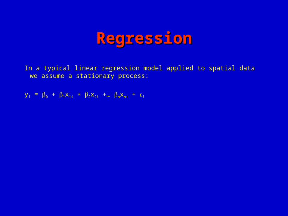
In a typical linear regression model applied to spatial data we assume a stationary process:

yi = 0 + 1x1i + 2x2i +… nxni + i

so that...so that...

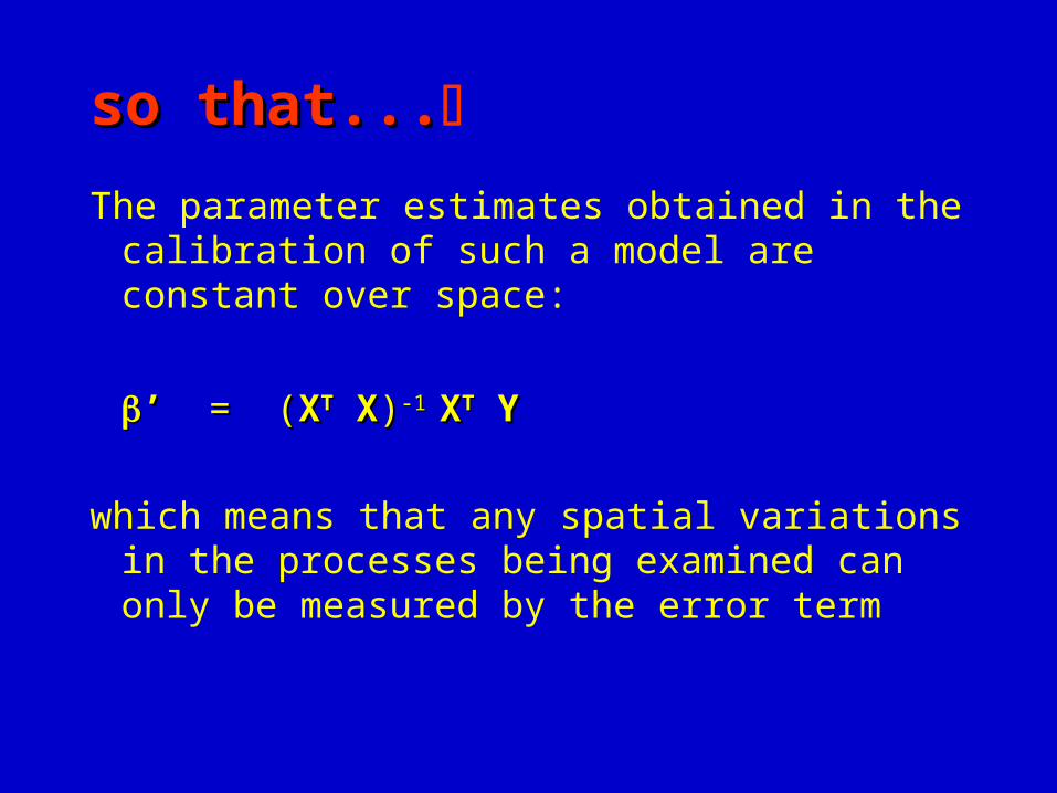
The parameter estimates obtained in the calibration of such a model are constant over space:

’ ’ = (= (XXTT X X))-1 -1 XXTT Y Y

which means that any spatial variations in the processes being examined can only be measured by the error term

Consequently...Consequently...

• We might map the residuals from the regression to determine whether there are any spatial patterns.

• Or compute an autocorrelation statistic

• We might even try to ‘model’ the error dependency with various types of spatial regression models.

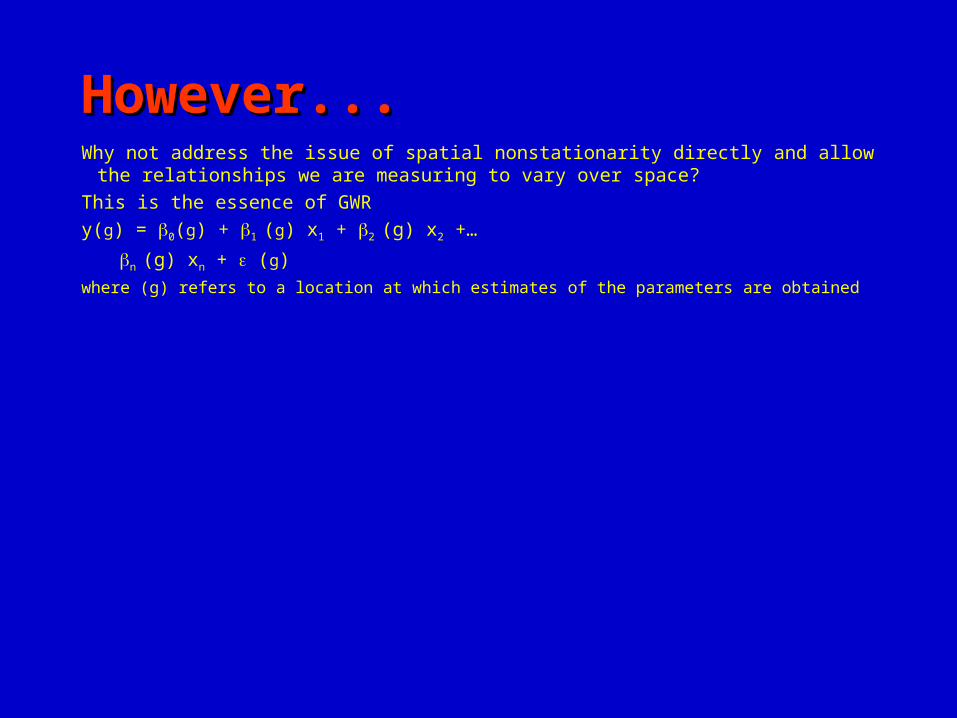
However...However...Why not address the issue of spatial nonstationarity directly and allow the

relationships we are measuring to vary over space?This is the essence of GWRy(g) = 0(g) + 1 (g) x1 + 2 (g) x2 +…

n (g) xn + (g)where (g) refers to a location at which estimates of the parameters are obtained

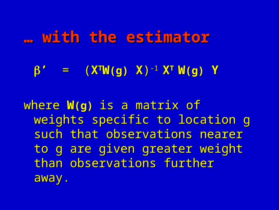
… … with the estimatorwith the estimator

’ ’ = (= (XXTTWW(g)(g) X X))-1 -1 XXT T WW(g)(g) Y Y

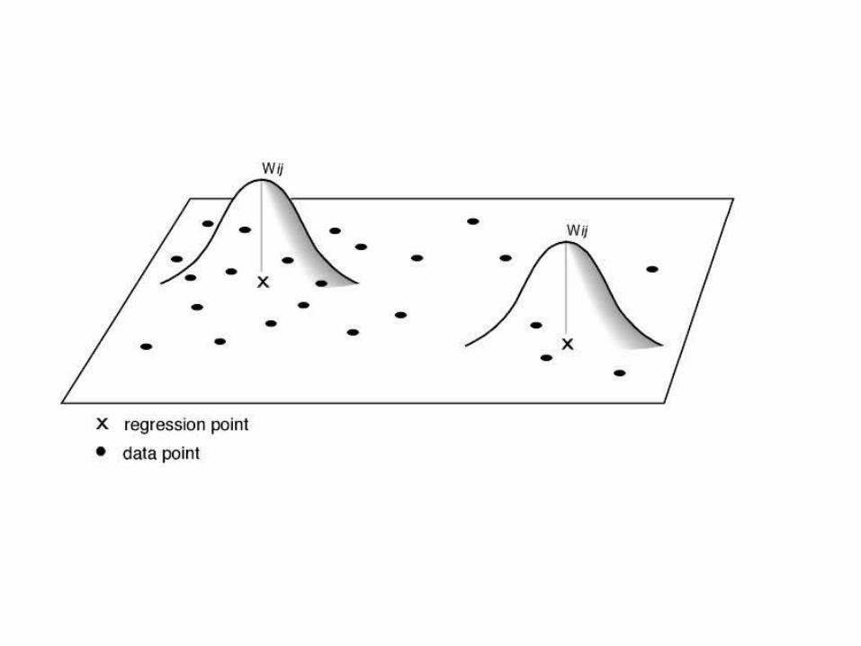
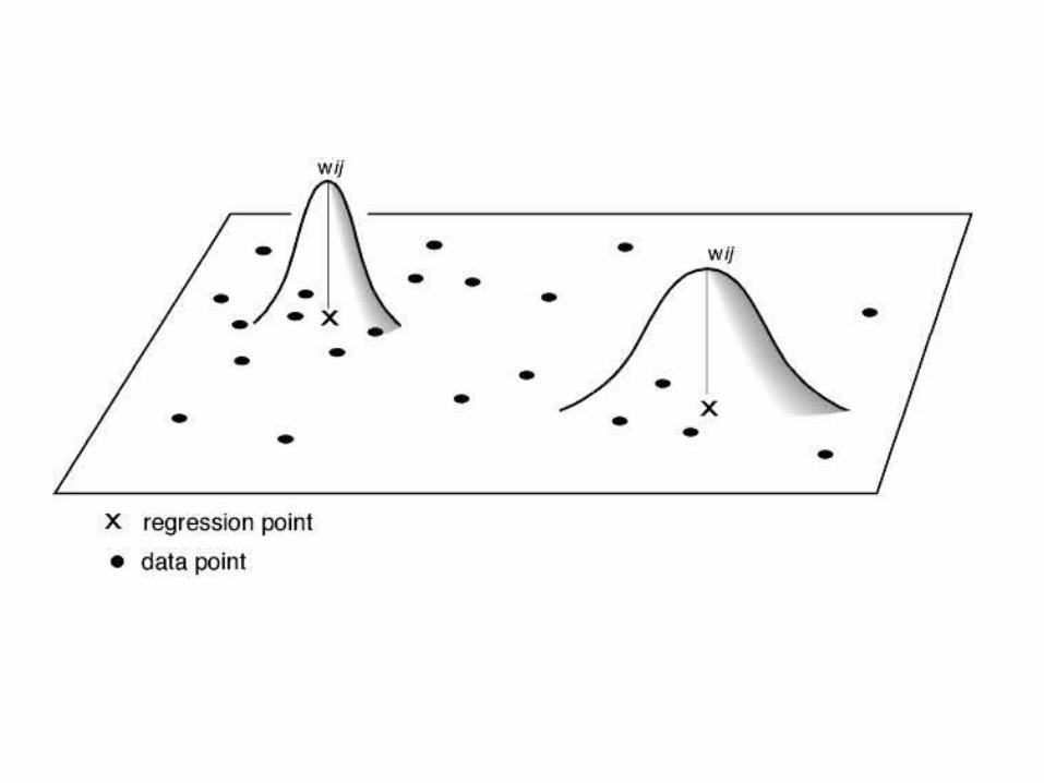
where where WW(g) (g) is a matrix of weights is a matrix of weights specific to location g such that specific to location g such that observations nearer to g are given observations nearer to g are given greater weight than observations greater weight than observations further away.further away.

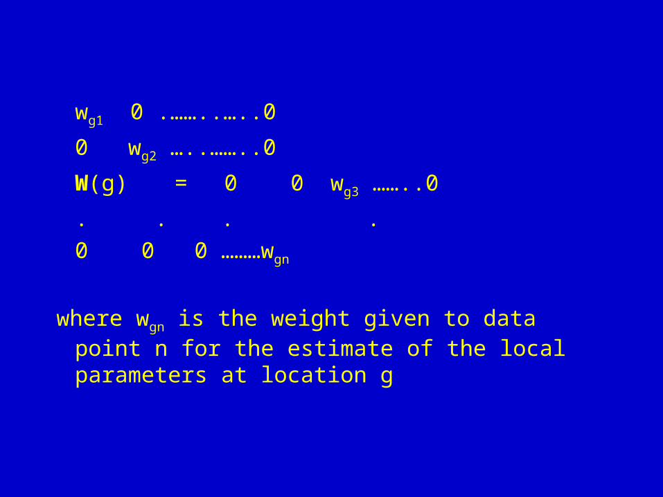
wg1 0 .……..…..0

0 wg2 …..……..0

W(g) = 0 0 wg3 ……..0

. . . .0 0 0 ………wgn

where wgn is the weight given to data point n for the estimate of the local parameters at location g

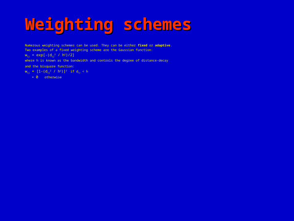
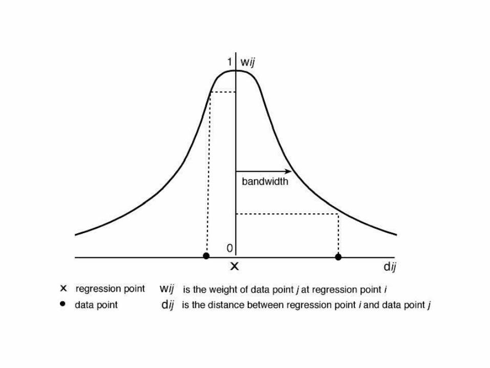
Weighting schemesWeighting schemesNumerous weighting schemes can be used. They can be either fixedfixed or adaptiveadaptive. Two examples of a fixed weighting scheme are the Gaussian function:

wij = exp[-(dij2 / h2)/2]

where h is known as the bandwidth and controls the degree of distance-decay

and the bisquare function:

wij = [1-(dij2 / h2)]2 if dij < h

= 0 otherwise

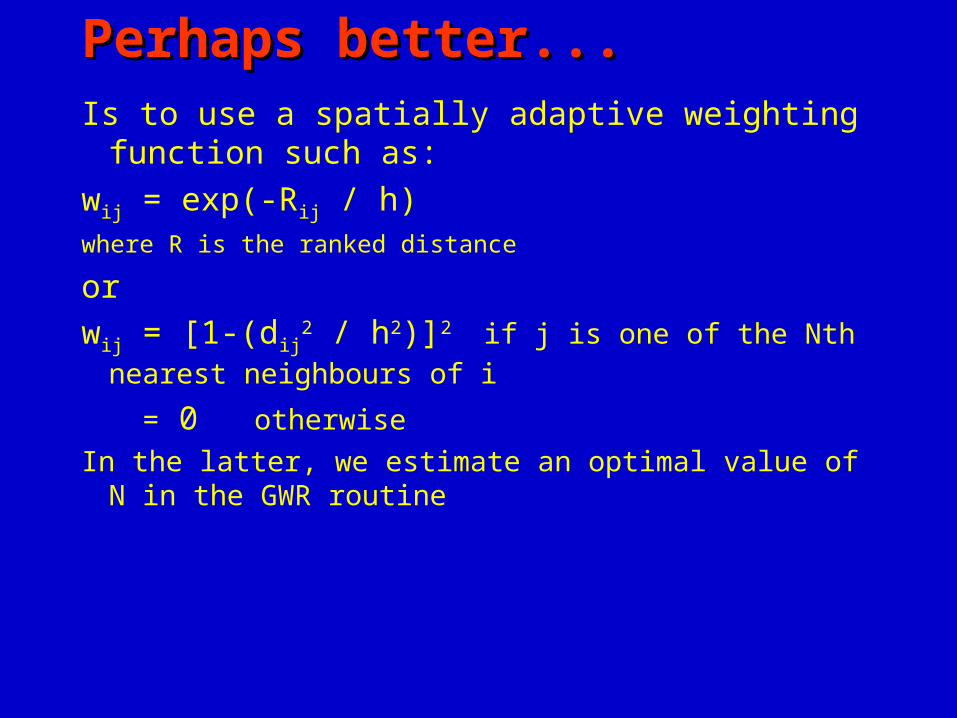
Perhaps better...Perhaps better...Is to use a spatially adaptive weighting

function such as:wij = exp(-Rij / h) where R is the ranked distance

orwij = [1-(dij

2 / h2)]2 if j is one of the Nth nearest neighbours of i

= 0 otherwise In the latter, we estimate an optimal value of N in the

GWR routine

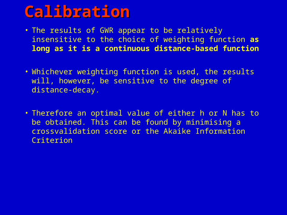
CalibrationCalibration• The results of GWR appear to be relatively insensitive

to the choice of weighting function as long as it is a continuous distance-based function

• Whichever weighting function is used, the results will, however, be sensitive to the degree of distance-decay.

• Therefore an optimal value of either h or N has to be obtained. This can be found by minimising a crossvalidation score or the Akaike Information Criterion

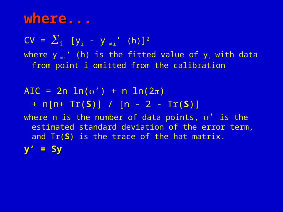
where...where...CV = i [yi - y i’ (h)]2

where y i’ (h) is the fitted value of yi with data from point i omitted from the calibration

AIC = 2n ln(’) + n ln(2) + n[n+ Tr(SS)] / [n - 2 - Tr(SS)]

where n is the number of data points, ’ is the estimated standard deviation of the error term, and Tr(SS) is the trace of the hat matrix.

y’ = Syy’ = Sy

GWR JargonGWR Jargon

• Sample pointsSample points– locations at which your data are measured

• Regression pointsRegression points– locations at which you require parameter

estimates

These need not be the same locationsThis can be handy if you want to map the

results from very large data sets

In GWR, we can also ...In GWR, we can also ...• estimate local standard errors• derive local t statistics• calculate local goodness-of-fit measures• calculate local leverage measures• perform tests to assess the significance of the

spatial variation in the local parameter estimates

• perform tests to determine if the local model performs better than the global one, accounting for differences in degrees of freedom

Software for GWR (GWR Software for GWR (GWR 2.0)2.0)

• User-friendly and menu-driven

• Provide a range of options

• Provide some helpful diagnostics

• Provide results for other software

The architecture of GWR The architecture of GWR 2.02.0• Currently about 3000 lines of FORTRAN

• VB front-end to create a control file and run the program

• Can run FORTRAN code under Unix with a control file or, more easily, by using the VB model editor in Windows (95; 98; ME)

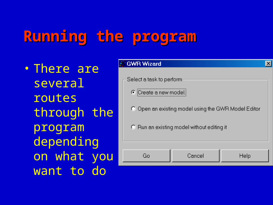
Running the programRunning the program

• There are several routes through the program depending on what you want to do

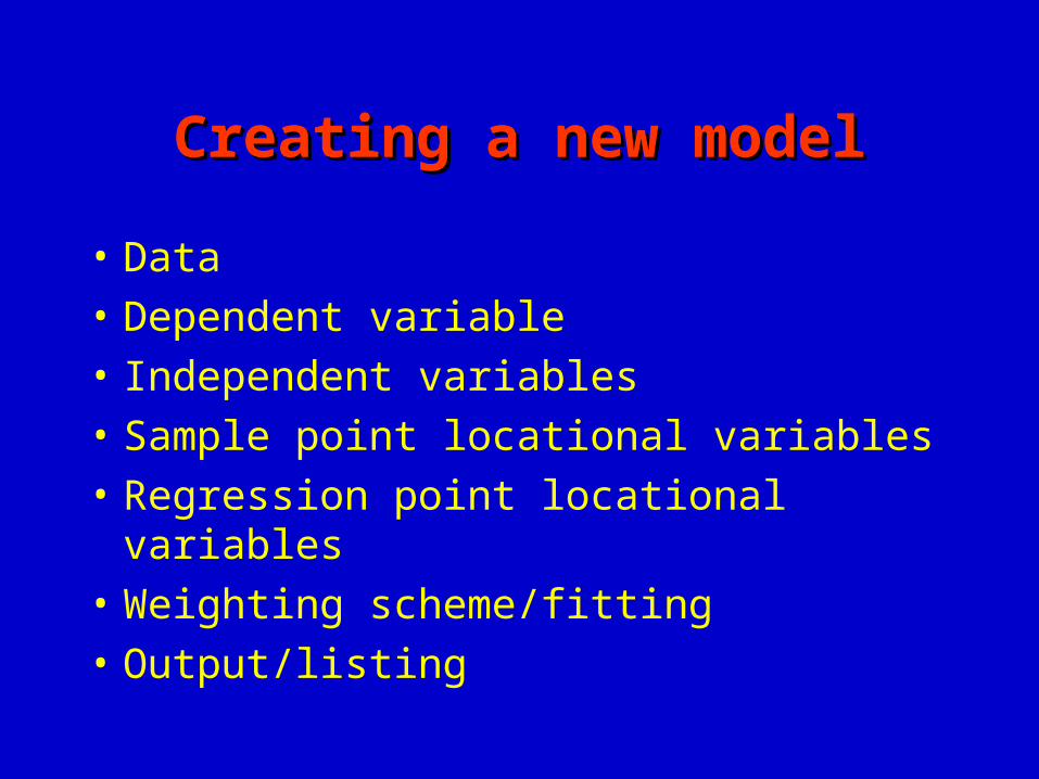
Creating a new modelCreating a new model

• Data• Dependent variable• Independent variables• Sample point locational variables• Regression point locational variables• Weighting scheme/fitting• Output/listing

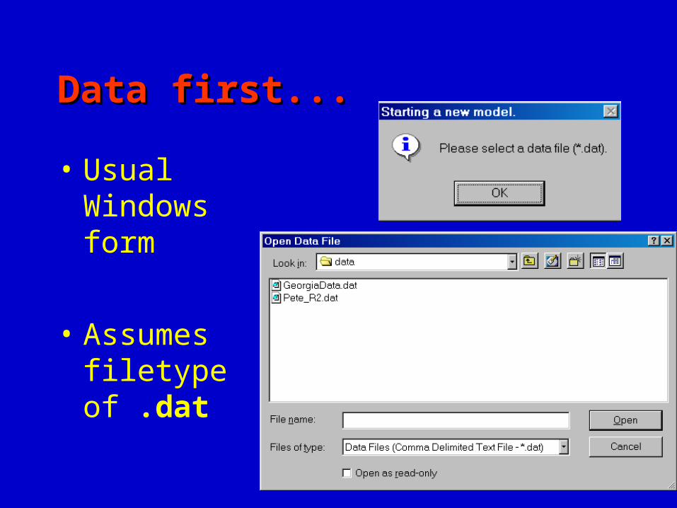
Data first...Data first...

• Usual Windows form

• Assumes filetype of .dat

Data structureData structure

• First line is a comma separated list of variable names (<= 8 characters)

• Data lines have numeric items only terminated by a carriage return

• One line of data per location• Space or comma delimited (easily

imported)

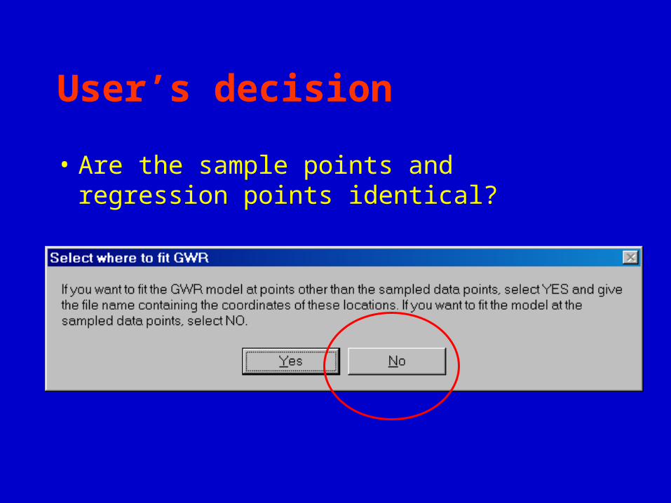
User’s decision

• Are the sample points and regression points identical?

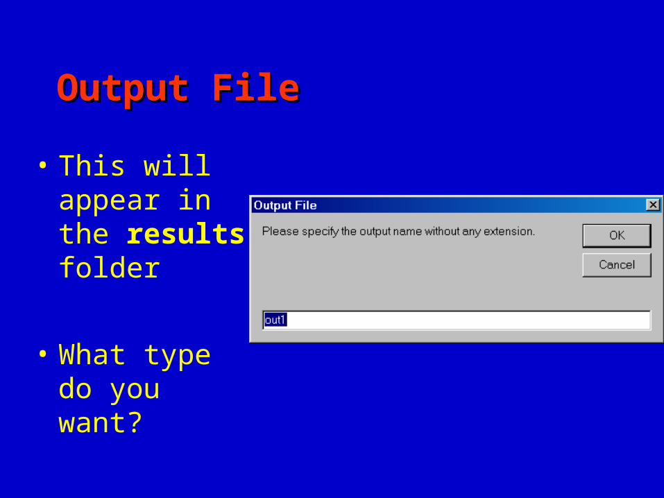
Output FileOutput File

• This will appear in the results folder

• What type do you want?

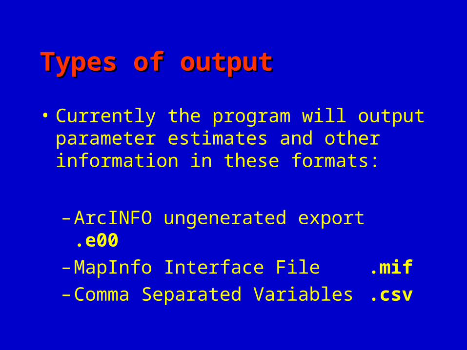
Types of outputTypes of output

• Currently the program will output parameter estimates and other information in these formats:

– ArcINFO ungenerated export .e00– MapInfo Interface File .mif– Comma Separated Variables .csv

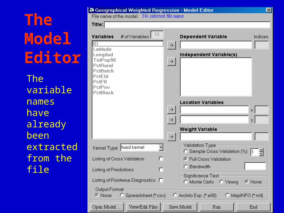
The Model EditorThe variable names have already been extracted from the file

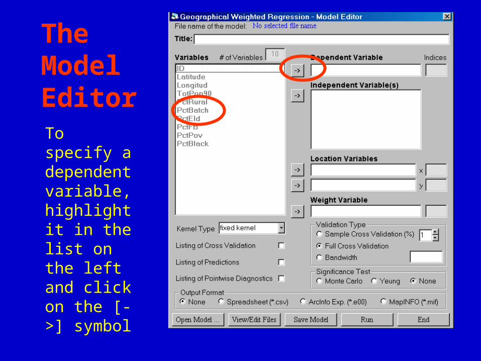
The Model EditorTo specify a dependent variable, highlight it in the list on the left and click on the [->] symbol

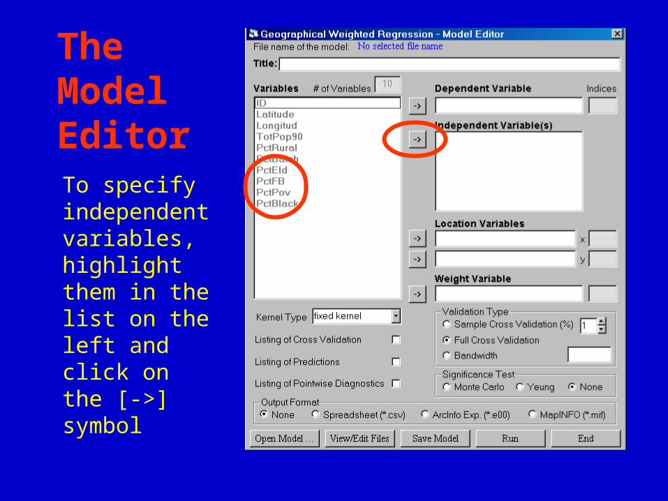
The Model EditorTo specify independent variables, highlight them in the list on the left and click on the [->] symbol

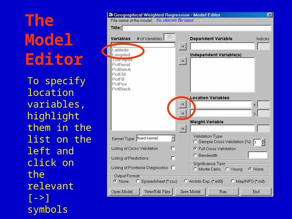
The Model EditorTo specify location variables, highlight them in the list on the left and click on the relevant [->] symbols

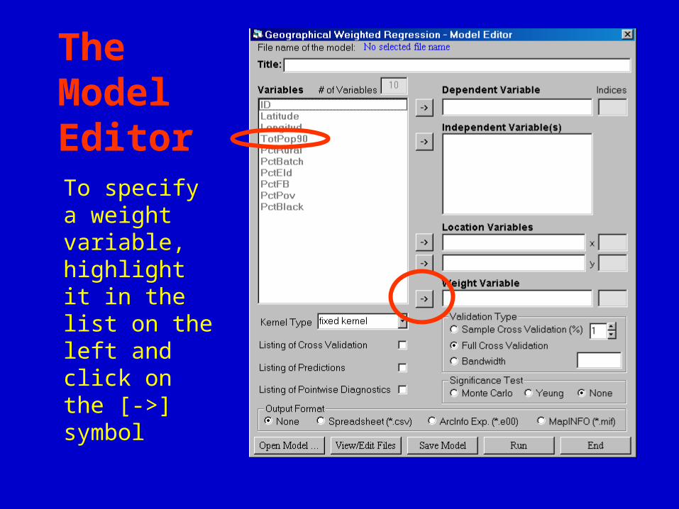
The Model EditorTo specify a weight variable, highlight it in the list on the left and click on the [->] symbol

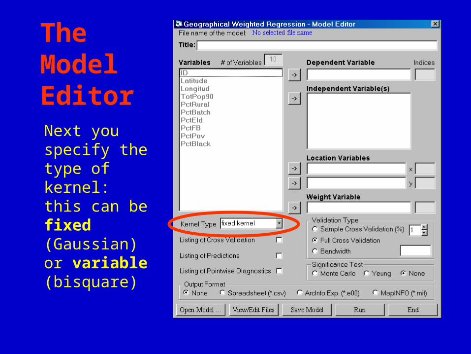
The Model EditorNext you specify the type of kernel: this can be fixed (Gaussian) or variable (bisquare)

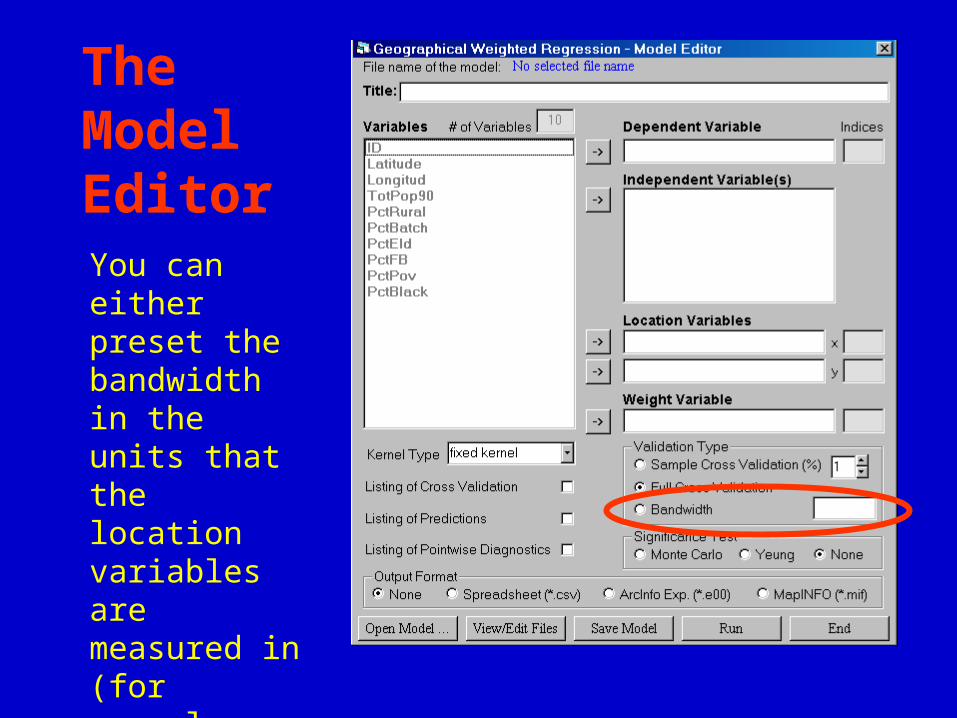
The Model EditorYou can either preset the bandwidth in the units that the location variables are measured in (for example, metres)

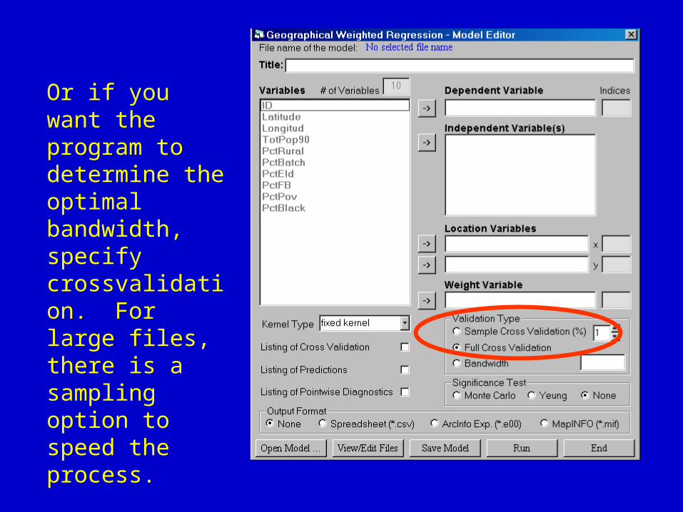
Or if you want the program to determine the optimal bandwidth, specify crossvalidation. For large files, there is a sampling option to speed the process.

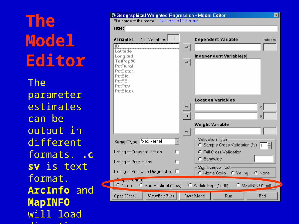
The Model EditorThe parameter estimates can be output in different formats. .csv is text format. ArcInfo and MapINFO will load directly.

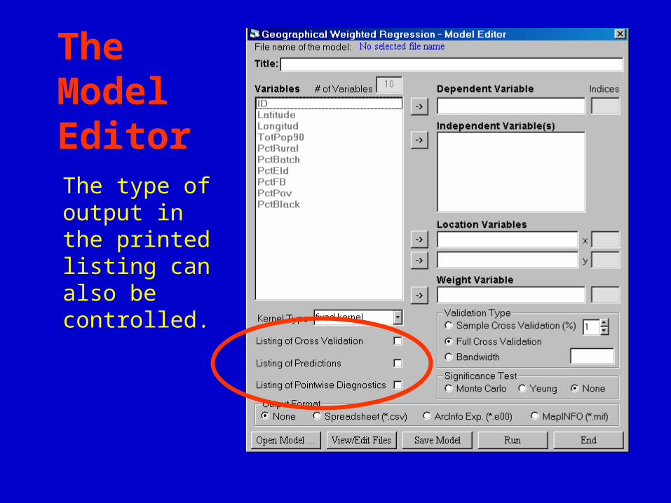
The Model EditorThe type of output in the printed listing can also be controlled.

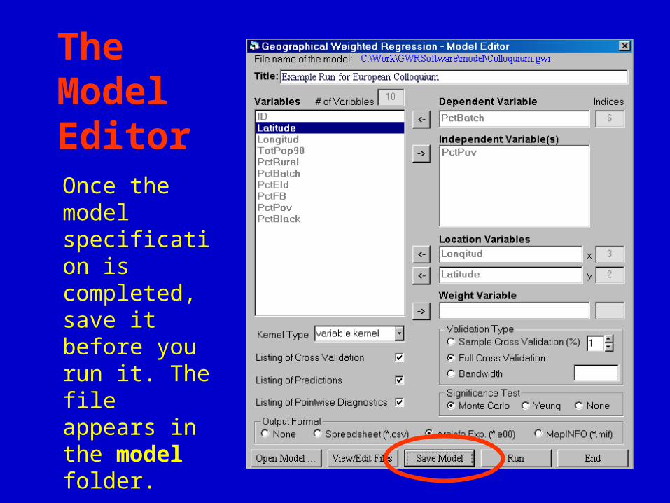
The Model EditorOnce the model specification is completed, save it before you run it. The file appears in the model folder.

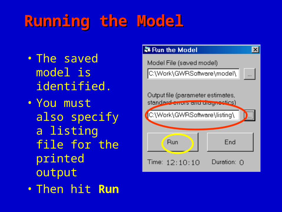
Running the ModelRunning the Model

• The saved model is identified.

• You must also specify a listing file for the printed output

• Then hit Run

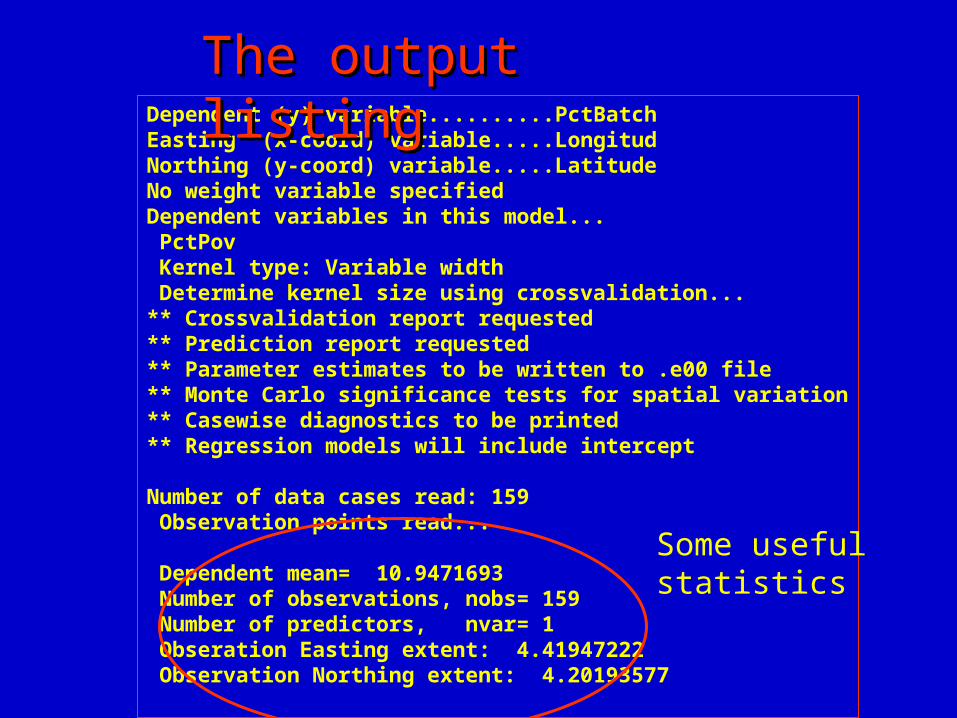
Dependent (y) variable..........PctBatchEasting (x-coord) variable.....LongitudNorthing (y-coord) variable.....LatitudeNo weight variable specifiedDependent variables in this model... PctPov Kernel type: Variable width Determine kernel size using crossvalidation...** Crossvalidation report requested** Prediction report requested** Parameter estimates to be written to .e00 file** Monte Carlo significance tests for spatial variation** Casewise diagnostics to be printed** Regression models will include intercept

Number of data cases read: 159 Observation points read... Dependent mean= 10.9471693 Number of observations, nobs= 159 Number of predictors, nvar= 1 Obseration Easting extent: 4.41947222 Observation Northing extent: 4.20193577

The output listingThe output listing

Some useful statistics

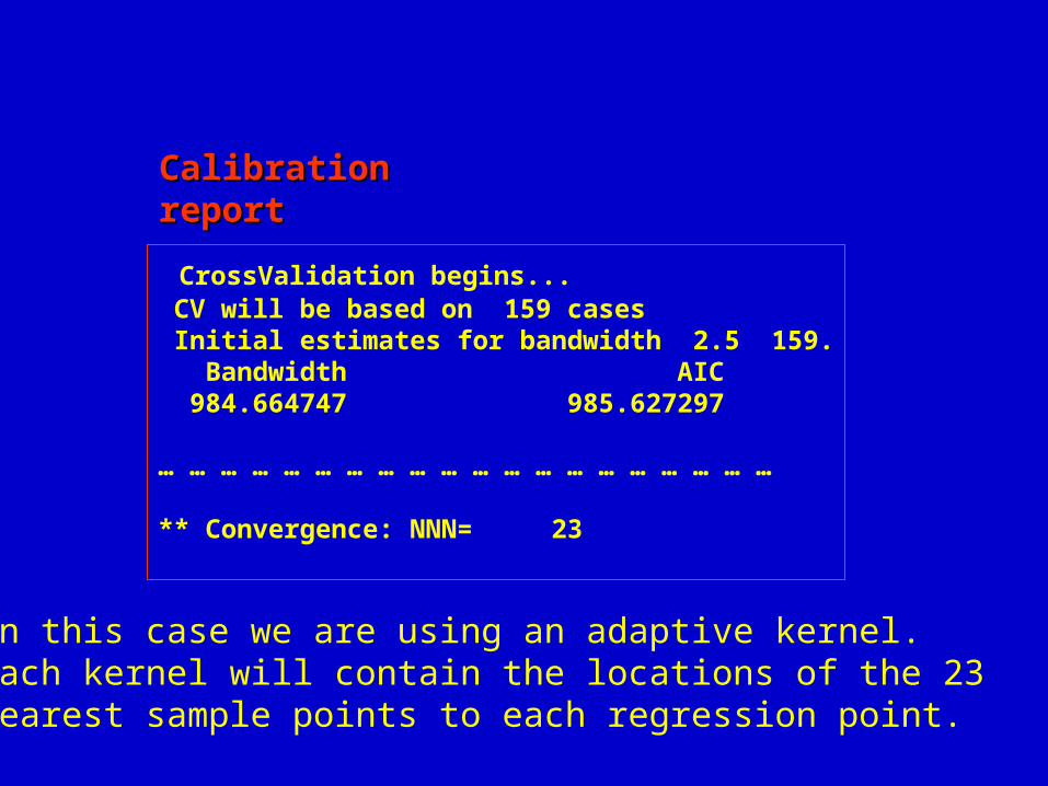
CrossValidation begins... CV will be based on 159 cases Initial estimates for bandwidth 2.5 159. Bandwidth AIC 984.664747 985.627297

… … … … … … … … … … … … … … … … … … … …

** Convergence: NNN= 23

Calibration reportCalibration report

In this case we are using an adaptive kernel.Each kernel will contain the locations of the 23nearest sample points to each regression point.

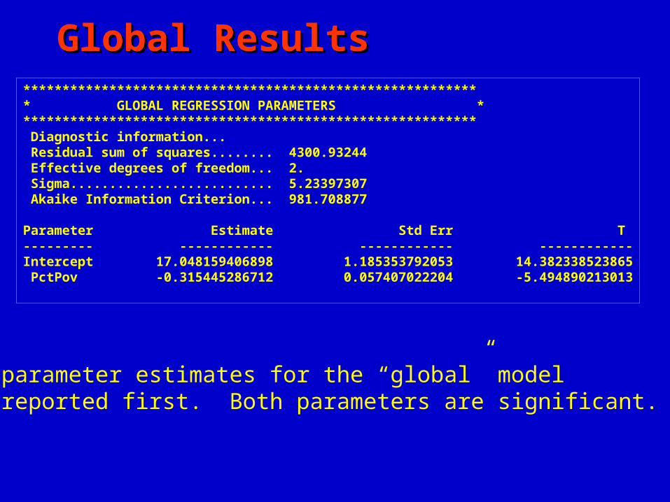
*********************************************************** GLOBAL REGRESSION PARAMETERS *********************************************************** Diagnostic information... Residual sum of squares........ 4300.93244 Effective degrees of freedom... 2. Sigma.......................... 5.23397307 Akaike Information Criterion... 981.708877

Parameter Estimate Std Err T--------- ------------ ------------ ------------Intercept 17.048159406898 1.185353792053 14.382338523865 PctPov -0.315445286712 0.057407022204 -5.494890213013

The parameter estimates for the “global” modelare reported first. Both parameters are significant.

Global ResultsGlobal Results

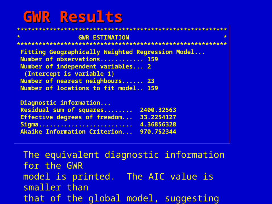
*********************************************************** GWR ESTIMATION *********************************************************** Fitting Geographically Weighted Regression Model... Number of observations............ 159 Number of independent variables... 2 (Intercept is variable 1) Number of nearest neighbours...... 23 Number of locations to fit model.. 159 Diagnostic information... Residual sum of squares........ 2400.32563 Effective degrees of freedom... 33.2254127 Sigma.......................... 4.36856328 Akaike Information Criterion... 970.752344

The equivalent diagnostic information for the GWRmodel is printed. The AIC value is smaller thanthat of the global model, suggesting that the GWRmodel is “better”.

GWR ResultsGWR Results

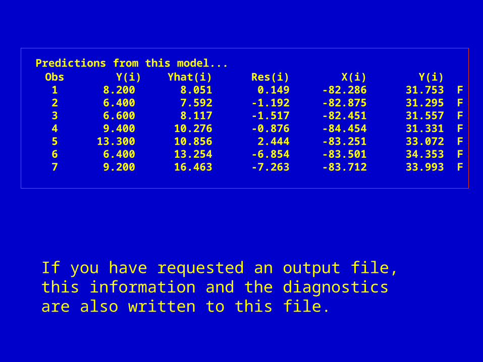
Predictions from this model... Obs Y(i) Yhat(i) Res(i) X(i) Y(i) 1 8.200 8.051 0.149 -82.286 31.753 F 2 6.400 7.592 -1.192 -82.875 31.295 F 3 6.600 8.117 -1.517 -82.451 31.557 F 4 9.400 10.276 -0.876 -84.454 31.331 F 5 13.300 10.856 2.444 -83.251 33.072 F 6 6.400 13.254 -6.854 -83.501 34.353 F 7 9.200 16.463 -7.263 -83.712 33.993 F

If you have requested an output file, this information and the diagnostics are also written to this file.

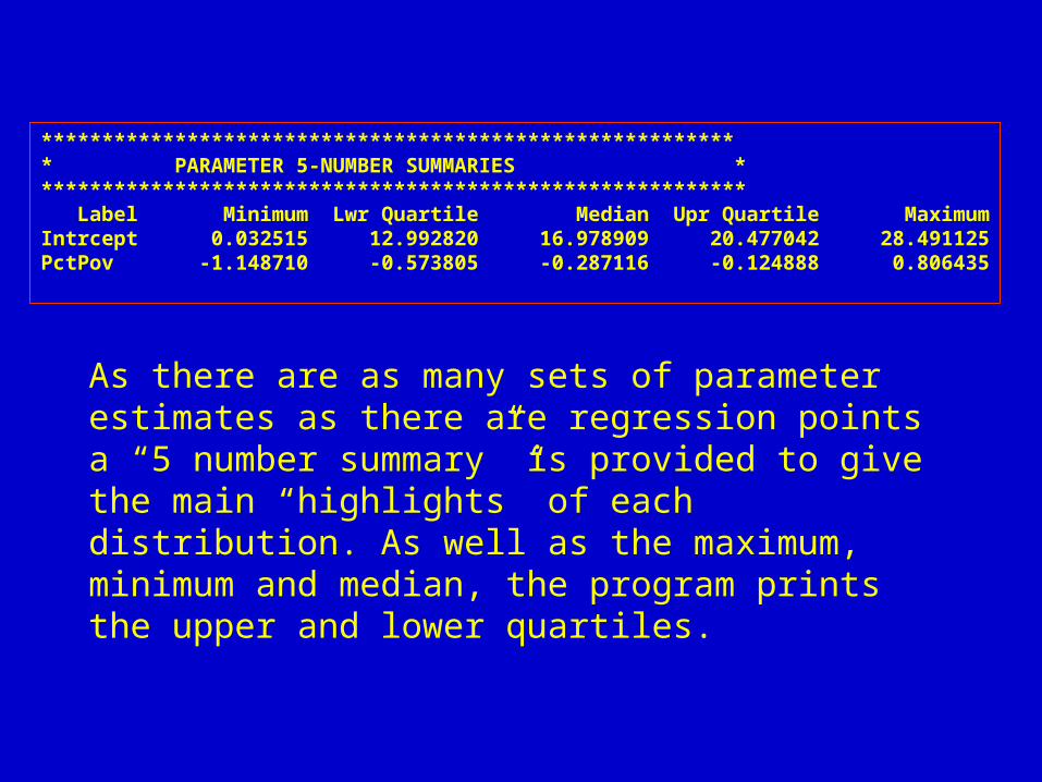
********************************************************** PARAMETER 5-NUMBER SUMMARIES *********************************************************** Label Minimum Lwr Quartile Median Upr Quartile MaximumIntrcept 0.032515 12.992820 16.978909 20.477042 28.491125PctPov -1.148710 -0.573805 -0.287116 -0.124888 0.806435

As there are as many sets of parameter estimates as there are regression points a “5 number summary” is provided to give the main “highlights” of each distribution. As well as the maximum, minimum and median, the program prints the upper and lower quartiles.

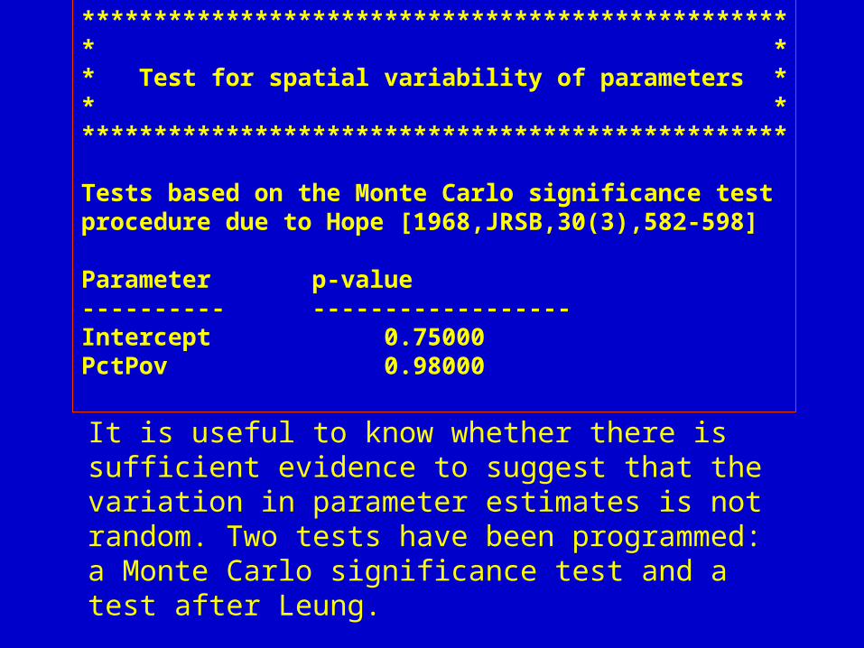
************************************************** ** Test for spatial variability of parameters ** ************************************************** Tests based on the Monte Carlo significance test procedure due to Hope [1968,JRSB,30(3),582-598] Parameter p-value---------- ------------------Intercept 0.75000PctPov 0.98000

It is useful to know whether there is sufficient evidence to suggest that the variation in parameter estimates is not random. Two tests have been programmed: a Monte Carlo significance test and a test after Leung.

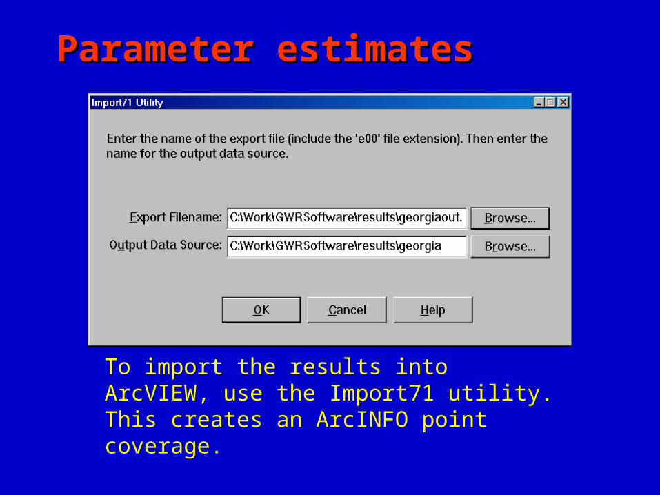
To import the results into ArcVIEW, use the Import71 utility. This creates an ArcINFO point coverage.

Parameter estimatesParameter estimates

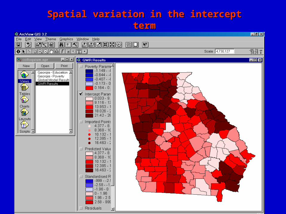
Spatial variation in the intercept Spatial variation in the intercept termterm

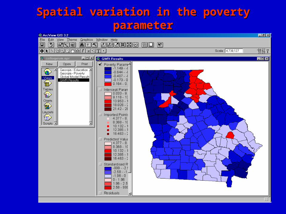
Spatial variation in the poverty Spatial variation in the poverty parameterparameter

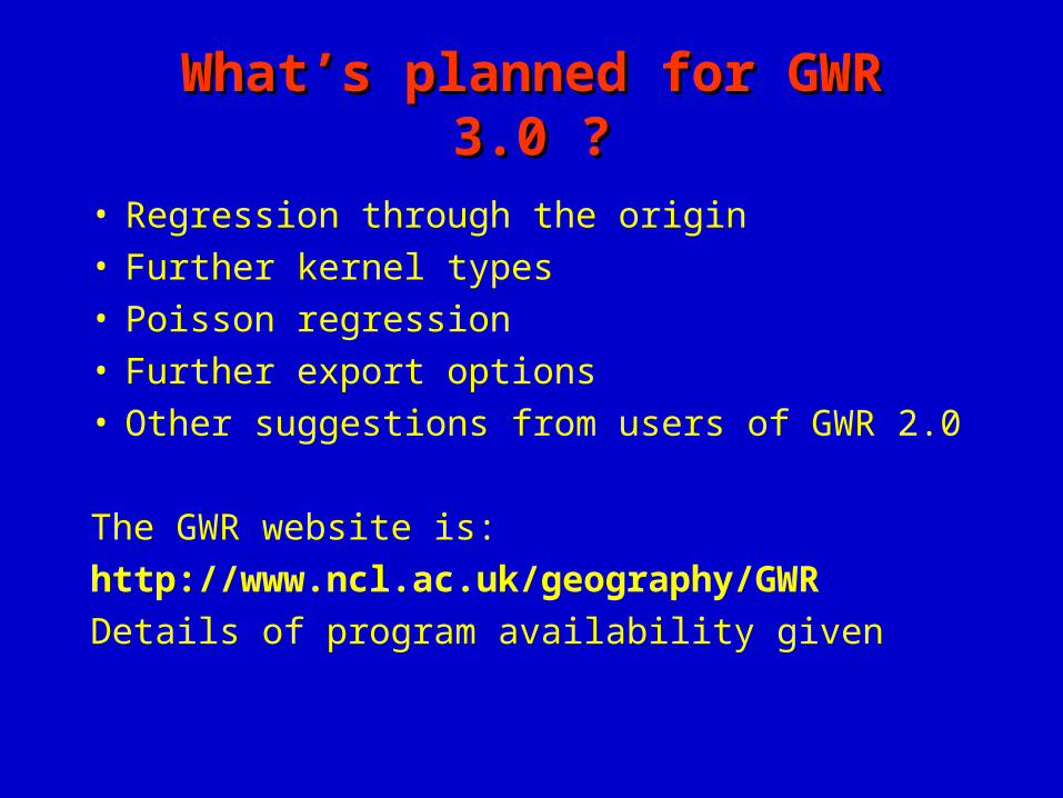
What’s planned for GWR What’s planned for GWR 3.0 ?3.0 ?

• Regression through the origin• Further kernel types• Poisson regression• Further export options• Other suggestions from users of GWR 2.0

The GWR website is:http://www.ncl.ac.uk/geography/GWRDetails of program availability given