Solar energy; the solution for the rising electricity demand?

1

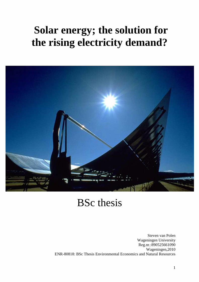
Solar energy; the solution for the rising electricity demand?

BSc thesis

Steven van Polen Wageningen University Reg.nr.:890525661090

Wageningen,2010 ENR-80818: BSc Thesis Environmental Economics and Natural Resources

2

Foreword Three years ago I finished high school, where all classes were obligatory. Some courses were interesting and others I just finished because I had to. At the University of Wageningen most of the courses are so interesting that even if they were not obligatory I would attend them. I think this is what they call internal motivation. It can be said that economics and policy is the study I always wanted to do. The environment in combination with economics always had my interest. This study gave me the opportunity to combine these two interesting topics. Theory and practice are combined which makes it very interesting. In this thesis the option for the production of Concentrated Solar Power (CSP) has been investigated. The basis is economics, but also the environment will play a major role. It will be the crowning glory of my last three years at Wageningen University. I would like to express my personal gratitude to prof.dr. van Ierland, my family friends and girlfriend. Prof.dr. van Ierland who always got me back on track, who gave me a lot of advice on how to build a model, which is the core of this thesis. My family and friends who helped me relax in times of stress. And last but certainly not least I would like to thank my girlfriend, who has always been there for me.

3

Abstract

All over the world temperatures are rising due to the greenhouse gas effect. It has been proven difficult to do something about greenhouse gas effect because it’s so widespread. A possibility to reduce the amount of greenhouse gas is solar energy. Solar energy is a renewable energy where the power of the sun is transformed in electricity.

Solar panels have different levels of effectiveness on different places in the world. The effectiveness depends on the amount of sun (hours and intensity). Also the political factors and the transport distance of the electricity should be taken into account. The General Algebraic Modelling System (GAMS) is used to determine the most accurate location for the solar panels. The compared countries are Algeria, Libya and Saudi Arabia.

The most effective way to reduce emissions is through a price on emissions. Price forecasts for fossil fuels show that the price of fossil fuels will rise. This will make it more attractive to produce CSP.

It can be concluded that the most effective location to place the solar panels will be Algeria. This because of the lowest transport costs and minor political hazards.

4

Table of contents Chapter Page number Foreword................................................................................... 2 Abstract………………………………………………………. 3 Table of contents……………………………………………… 4 1. Introduction………………………………………………... 5 2. Theory and modelling……………………………………... 7 3. Description of the GAMS model………………………….. 9 4. Data description…………………………………………… 15 5. Scenarios…………………………………………………... 21 6. Conclusion………………………………………………… 46 References…………………………………………………… 48 Appendices………………………………………………….. 51

5

1. Introduction

There are many investigations on the relation between the rising temperature and the amount of greenhouse gases in the air. Most investigations have the outcome that temperatures will raise for the coming 40 years to at least an increase of two degrees Celsius. With this rise there will be some changes in climate but the changes are acceptable. The problem only is that we have to emit a lot less greenhouse gasses to reach this acceptable norm of two degrees Celsius. A prominent solution to reduce these emissions are solar panels (PV), these are panels that turn solar energy in electricity.

To make these solar panels (PV) profitable a huge amount of space is needed. With the technology of the Concentrating Solar Panels (CSP) the amount of space needed will be smaller, because the technology will make the heat a lot more intense and therefore more electricity can be generated with the solar panels. But CSP still needs a huge amount of space to generate electricity. A foundation that already investigated different regions to place these CSP is the Desertec foundation, this foundation looks at the possibility of producing energy in North Africa, Middle East and Europe. One form of electricity generation where the Desertec foundation looks at is CSP. After research they have selected several suitable regions for such CSP sites [RNW, 2009]. The objective of the Desertec foundation is to generate a big part of Europe’s electricity by using renewable sources such as solar energy. To reach this goal a lot of money is needed and this money can come from governments and private investors. But the projects of this foundation have to be financially attractive for both these actors because otherwise they will not invest in the projects.

In this thesis a comparison is made between three different regions that have suitable regions for CSP sites according to the Desertec foundation. The countries that will be compared are Algeria, Libya and Saudi Arabia which are all countries with different political and economical backgrounds. These backgrounds influence the attractiveness for the actors that have to invest in the different projects.

A GAMS model has been created to investigate which of the three countries is the most interesting for the investors. This GAMS model will compare the three countries, further also three energy sources are compared namely gas, coal and CSP. A time period is also included, this will start in the year 2000 and the end of the time period is 2050. These are the sets in the model, the factors that are described by the model. But there are other factors that influence these sets because not every factor in this set has the same impact. For example energy sources will emit different amounts of emissions when electricity is produced. These sets are influenced by many different factors but these could not all be included in this model. The factors that are included in this model are the market forces, loss of electricity when transported, amount of electricity wire needed to reach the European market, political influence and the costs of emissions. The goal of this model is to find the lowest amount of costs used to generate the amount of electricity demanded.

This model will help to answer the research questions, the main research question in this research is to answer which region is most suitable to place solar panels in a cost-efficient way and/or emit the lowest amount of emissions? This will be answered by answering the sub-research questions, the first one is about which region can deliver energy from solar panels to Europe with the lowest costs? This one will be answered by the model, then the model will be used again to describe how high the costs will be when the emissions are as low as possible, this is the second sub-research question. The certainty of supply is included in the model but the general political culture of the country will also play a role in this research, this is the subject where the third research question will focus on. The main research question will be answered while taking into account all the other research questions.

6

This thesis has been written as BSc thesis and I had to make many assumptions. Although I collected the best available information, the reader should be aware that the study does not provide results that can be directly implied in policymaking. For that much more in depth research is required. There is one special assumption and this is about the available energy sources in the three countries compared. The assumption is that every country can produce coal, gas or CSP while in reality the countries do not have all these energy sources.

7

2. Theory and modelling

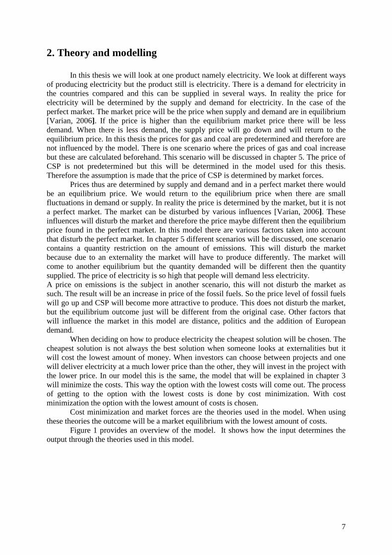
In this thesis we will look at one product namely electricity. We look at different ways of producing electricity but the product still is electricity. There is a demand for electricity in the countries compared and this can be supplied in several ways. In reality the price for electricity will be determined by the supply and demand for electricity. In the case of the perfect market. The market price will be the price when supply and demand are in equilibrium [Varian, 2006]. If the price is higher than the equilibrium market price there will be less demand. When there is less demand, the supply price will go down and will return to the equilibrium price. In this thesis the prices for gas and coal are predetermined and therefore are not influenced by the model. There is one scenario where the prices of gas and coal increase but these are calculated beforehand. This scenario will be discussed in chapter 5. The price of CSP is not predetermined but this will be determined in the model used for this thesis. Therefore the assumption is made that the price of CSP is determined by market forces. Prices thus are determined by supply and demand and in a perfect market there would be an equilibrium price. We would return to the equilibrium price when there are small fluctuations in demand or supply. In reality the price is determined by the market, but it is not a perfect market. The market can be disturbed by various influences [Varian, 2006]. These influences will disturb the market and therefore the price maybe different then the equilibrium price found in the perfect market. In this model there are various factors taken into account that disturb the perfect market. In chapter 5 different scenarios will be discussed, one scenario contains a quantity restriction on the amount of emissions. This will disturb the market because due to an externality the market will have to produce differently. The market will come to another equilibrium but the quantity demanded will be different then the quantity supplied. The price of electricity is so high that people will demand less electricity. A price on emissions is the subject in another scenario, this will not disturb the market as such. The result will be an increase in price of the fossil fuels. So the price level of fossil fuels will go up and CSP will become more attractive to produce. This does not disturb the market, but the equilibrium outcome just will be different from the original case. Other factors that will influence the market in this model are distance, politics and the addition of European demand. When deciding on how to produce electricity the cheapest solution will be chosen. The cheapest solution is not always the best solution when someone looks at externalities but it will cost the lowest amount of money. When investors can choose between projects and one will deliver electricity at a much lower price than the other, they will invest in the project with the lower price. In our model this is the same, the model that will be explained in chapter 3 will minimize the costs. This way the option with the lowest costs will come out. The process of getting to the option with the lowest costs is done by cost minimization. With cost minimization the option with the lowest amount of costs is chosen. Cost minimization and market forces are the theories used in the model. When using these theories the outcome will be a market equilibrium with the lowest amount of costs.

Figure 1 provides an overview of the model. It shows how the input determines the output through the theories used in this model.

8

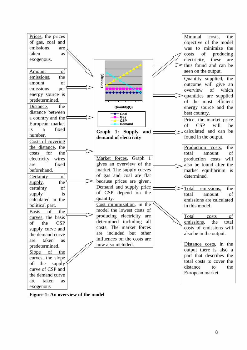
Figure 1: An overview of the model

Prices, the prices of gas, coal and emissions are taken as exogenous.

Amount of emissions, the amount of emissions per energy source is predetermined. Distance, the distance between a country and the European market is a fixed number. Costs of covering the distance, the costs for the electricity wires are fixed beforehand. Certainty of supply, the certainty of supply is calculated in the political part. Basis of the curves, the basis of the CSP supply curve and the demand curve are taken as predetermined. Slope of the curves, the slope of the supply curve of CSP and the demand curve are taken as exogenous

Quantity(Q)

Pri

ces(

p)

CoalGasCSPDemand

Graph 1: Supply and demand of electricity

Market forces, Graph 1 gives an overview of the market. The supply curves of gas and coal are flat because prices are given. Demand and supply price of CSP depend on the quantity. Cost minimization, in the model the lowest costs of producing electricity are determined including all costs. The market forces are included but other influences on the costs are now also included.

Minimal costs, the objective of the model was to minimize the costs of producing electricity, these are thus found and can be seen on the output.

Quantity supplied, the outcome will give an overview of which quantities are supplied of the most efficient energy source and the best country. Price, the market price of CSP will be calculated and can be found in the output.

Production costs, the total amount of production costs will also be found after the market equilibrium is determined.

Total emissions, the total amount of emissions are calculated in this model.

Total costs of emissions, the total costs of emissions will also be in the output.

Distance costs, in the output there is also a part that describes the total costs to cover the distance to the European market.

9

3. Description of the GAMS model GAMS and the model

The program used to model this research is the General Algebraic Modelling System (GAMS) [GAMS, 2010]. The GAMS is a program used to model many different forms of problems including the problem of Desertec. In this research GAMS is used for this purpose and how the program is used will be discussed in this chapter. In appendix [1], there is an example of a GAMS model used. Goal description of the model

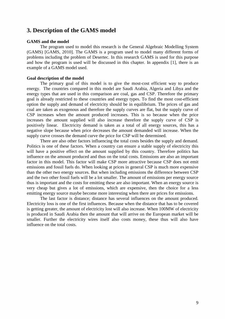
The primary goal of this model is to give the most-cost efficient way to produce energy. The countries compared in this model are Saudi Arabia, Algeria and Libya and the energy types that are used in this comparison are coal, gas and CSP. Therefore the primary goal is already restricted to these countries and energy types. To find the most cost-efficient option the supply and demand of electricity should be in equilibrium. The prices of gas and coal are taken as exogenous and therefore the supply curves are flat, but the supply curve of CSP increases when the amount produced increases. This is so because when the price increases the amount supplied will also increase therefore the supply curve of CSP is positively linear. Electricity demand is taken as a total of all energy sources, this has a negative slope because when price decreases the amount demanded will increase. When the supply curve crosses the demand curve the price for CSP will be determined.

There are also other factors influencing the total costs besides the supply and demand. Politics is one of these factors. When a country can ensure a stable supply of electricity this will have a positive effect on the amount supplied by this country. Therefore politics has influence on the amount produced and thus on the total costs. Emissions are also an important factor in this model. This factor will make CSP more attractive because CSP does not emit emissions and fossil fuels do. When looking at prices in general CSP is much more expensive than the other two energy sources. But when including emissions the difference between CSP and the two other fossil fuels will be a lot smaller. The amount of emissions per energy source thus is important and the costs for emitting these are also important. When an energy source is very cheap but gives a lot of emissions, which are expensive, then the choice for a less emitting energy source maybe become more interesting when there are prices for emissions.

The last factor is distance; distance has several influences on the amount produced. Electricity loss is one of the first influences. Because when the distance that has to be covered is getting greater, the amount of electricity lost will also increase. When 100MW of electricity is produced in Saudi Arabia then the amount that will arrive on the European market will be smaller. Further the electricity wires itself also costs money, these thus will also have influence on the total costs.

10

Variables for equations in algebraic form To give a more general idea about the equations used, these will be described in algebraic form now. In the description of the variables the bold variables are the sets used, further the variables are put in order of appearance. The variables used to put the equations in algebraic form are: I: The different countries (Algeria, Libya and Saudi Arabia) J: The different energy sources (Gas, Coal and CSP) T: Time (2000, 2010, 2020, 2030, 2040, 2050) Q: Amount of electricity produced AD: Total amount of Demand EurF: Fraction of European demand supplied by CSP producing countries EurT: Total European demand TdemE: Total electricity demand from Europe AS: Total amount of Supply GW_E: Amount of Gigawatt for each energy source per power plant Edem: total electricity demand from countries themselves Eloss: percentage of electricity loss per kilometre DisL: Distance that has to be covered over land to European market DisW: Distance that has to be covered through water to European market ElossC: percentage electricity loss over the whole distance TEloss: Total electricity loss Sd: Starting value of the demand curve Cd: Slope of the demand curve Pd: price of the electricity demand

Scsp: Starting value of the supply curve for CSP Ccsp: Slope of the CSP supply curve Pcsp: Price of CSP electricity supply AP: Total amount of production costs COS: Certainty of Supply Mcos: Minimum level of COS Gdep: dependency on gas Cdep: dependency on coal CSPdep: dependency on CSP Mdep: Minimum dependency level EfG: amount of emissions when producing gas EfC: amount of emissions when producing coal EfCSP: amount of emissions when producing CSP Em: Total amount of emissions PEm: Price of emissions ACE: total amount of costs for emissions CEL: Costs of electricity wires on land CEW: Costs of electricity wires through water ACD: Total amount of costs for covering the distance to the European market AC: Total amount of costs

11

The equations in algebraic form Now the equations themselves are introduced. The objective function over time contains a blue part of the formula. This blue part is included when there is a discount rate included in the model. It is excluded when there is no discount rate included in the model. The equations used in the model in algebraic form: Quantity demanded: QG,it + QC,it +QCSP,it= ADit

Demand from Europe EurFi*EurTi = TdemEi Total demand in GW Σt (Σj (ASit* GW_Ejt)) = Edemi+ TdemEi Percentage electricity loss Elosst*( DisL i+ DisWi)=ElossCi Total amount of electricity loss (ElossCi/100)* ADit=TElossij Balance supply and demand: AD it+ TElossij =ASit

Demand curve: Sdt-( Cdt* AD it)=Pdit Prices of CSP supply: (Scspit+( Ccspijt* QCSPit))*(1+(ElossCi/100))= Pcspit Equilibrium of prices: Pdit = Pcspit Total Costs for production in equilibrium: (QG,it*PG,it) + ( QC,it* PC,it) ) + ( QCSP,it* PCSP,it) = ATit Certainty of supply equation Σi (Σt ((QG,it* COSi) + ( QC,it*COSi) + ( QCSP,it* COSi))> Mcos Dependency on Russia equation Σi (Σt ((QG,it* Gdep i) + ( QC,it*Cdepi) + ( QCSP,it* CSPdepi)) > Mdep Emissions: (QG,it* EfGt) + ( QC,it*EfC t) + ( QCSP,it* EfCSPt)= Emit Costs of Emissions: Σj (Emit * PEmjt)=ACEit

Distance: (DisLi * CELi) + (DisWi * CEWi)= ACDi Objective function over time Σi ((ATit + ACEit + ACDi)*(1/ ((1+0.04) ^ ((t-1)*10))) =ACt Summation of total costs Σt(ACt)=AC

12

Description of GAMS model Sets In the model three sets are present. The first set represents the different energy sources taken into account in the model. The three countries compared in this research are the second set. The last set is the time set, with this set a time path between 2000 and 2050 is created. When a discount rate is used there is a small part explaining this in the set section. This describes that the first period is 2000 and the last is 2050. Scalars, parameters and tables Now the input of the model will be described. Tables contain more information the parameters, parameters contain more information then scalars. Scalars are not influenced by any set, these are just single numbers. Parameters are influenced by one set and thus are a row of numbers. Tables are influenced by two sets and therefore form a table of numbers. The first input is a table that describes the amount of GW produced per power plant (MW_P(E,T)) over time. Then we go to the parameter that describes the total electricity demand in GW (E_dem(C)) for each country that we compare. Then two parameters are discussed, the first two parameters are the parameters for the demand price curve. These are the starting price (B_D(T)) and the slope of the demand curve (P_E(T)) which determine the determine the demand price curve. The next parameter that will be discussed is the demand for electricity in Europe (Eur_D(C)). Total European demand is divided by three, this way each country has to produce one third of the electricity demand in Europe. Every country does not have to produce everything of this electricity demand. That is where the next parameter comes in, this describes the part of the electricity demand that the countries have to supply (EUR_P(C)). Then we go to the parameters for the different prices that are taken beforehand. These are the prices for gas (P_G(C,T)) and coal (P_C(C,T)). Further there is also a price for emissions (P_Em(E,T)) and this will increase over time. The price of CSP is determined by the model itself, therefore the supply of CSP is not determined beforehand. This is determined by a basic price (B_CSP(C,T)) and the slope of the curve(P_E(C,T)). There is also some political influence taken into account in this model. This is represented by the certainty of supply (COS(C,). A minimum of the certainty of supply is needed in the model. The countries have to be above this scalar and countries that are more stable are thus preferred over the others. This is not the only political influence, the dependency on gas (Gdep(T)) is another. We want to exchange this dependency for the dependency on CSP (CSPdep(T)) or coal (Cdep(T)). The urgency of this is determined by the scalar that describes the minimum level of this dependency (Tdep). Above there was a parameter which was the price of emissions, but the amount of emissions per form of raw material is determined beforehand. The amount of emission for coal (E_C(T)) is higher than the amount of emissions for gas (E-G(T)). The amount of emissions for CSP (E_CSP(T)) is the lowest. Distance is also included in the model. Distance over land (DisL(C)) and over water (DisW(C)) are described here. The costs for the electricity wires used on land (CdisL) and through water (CdisW) are the last scalars. The last parameter describes the percentage electricity loss over the distance travelled (Eloss(T)).

13

Variables The next part is about the variables used in the model. Quantities of the different raw materials and in which time and country are very important, these are represented by the first three variables. The three energy sources are described here, these thus are gas (vQ_G(C,T)), coal (vQ_C(C,T)) and CSP (vQ_CSP(C,T)). These quantities determine the amount of supply which is represented in the parameter (vT_D(C,T)). This should be equal to the amount demanded, this is represented in the parameter (vT_S(C,T)). But demand is not only determined by the demand of the countries itself, the demand for electricity (vT_DE(C)) from Europe is also important. The next variable is the price of the demand curve (vE_DP(C,T)) which should be equal to the price of the CSP supply curve (vESP_CSP(C,T)) of the different countries. When all these previous variables are determined the total costs of production can be determined (vTPC_T(C,T)). After this there are several other factors that influence the total costs. Emissions are another factor that has to be taken into account. First the total amount of emissions with production is determined (vT_E(C,T)). After this the total costs of emissions are calculated (vTEC(C,T)). Another factor that influences the total costs, are the total costs for covering the distance (vCDis(C)). This is not the only way in which distance influences total cost, the distance also influences the electricity loss (vEld(C,T)). First the percentage of electricity loss (vEl(C,T)) is calculated and then this multiplied by total demand and this is the electricity loss. The last two variables are about the total costs. First the total costs over time (vT_CoT(T)) are calculated, then these costs are summed up and the total costs (vT_C) are calculated. Equations as in the GAMS file In the equation for the total cost over time there is a blue part. The blue part represents the discount rate. When this in included the blue part is also included. When there is no discount rate the blue part is excluded. Function for quantity demand eDem(C,T).. (vQ_G(C,T)+vQ_C(C,T)+vQ_CSP(C,T))=E=vT_D(C,T); Demand from Europe eDemE(C).. (EUR_P(C)*Eur_D(C))=E=vT_DE(C); Demand in GW eDemandGW(C).. (SUM(T,SUM(E,((vT_S(C,T)*MW_P(E,T))))))=G=(E_dem(C)+vT_DE(C)); Percentage loss of electricity over the distance transported eEloss(C,T).. (Eloss(T)*(DisL(C)+DisW(C)))=E=vEl(C,T); Total amount lost of Demand eElossD(C,T).. ((vEl(C,T)/100)*vT_D(C,T))=E=vEld(C,T); Balance supply and demand: Here supply and demand are equalized bSD(C,T).. vT_D(C,T)+vEld(C,T)=E=vT_S(C,T); Demand curve: In this equation the demand price is determined eDemP(C,T).. (B_D(T)-(P_ED(T)*vT_D(C,T)))=E=vE_DP(C,T);

14

Prices of CSP supply: In this equation the supply price of CSP is determined epCSP(C,T).. ((B_CSP(C,T)+(vQ_CSP(C,T)*P_CSP(C,T))*(1+(vEl(C,T)/100))))=E=vESP_CSP(C,T); Equilibrium of prices: The CSP supply price and the demand price are equalized bEPSDCSP(C,T).. vESP_CSP(C,T)=E=vE_DP(C,T); Total Costs for production in equilibrium: Total costs for production are calculated eCprod(C,T).. (vQ_G(C,T)*P_G(C,T))+(vQ_C(C,T)*P_C(C,T))+(vQ_CSP(C,T)*vESP_CSP(C,T))=E=vTPC_T(C,T); Certainty of supply: Now the certainty of supply is introduced and the price is corrected for this. rPolinf.. ((SUM(T,SUM(C,(vQ_G(C,T)*COS(C))))))+(SUM(T,SUM(C,(vQ_C(C,T)*COS(C)))))+(SUM(T,SUM(C,(vQ_CSP(C,T)*COS(C)))))=G=GL; Including the dependency of different countries rdependency.. ((SUM(T,SUM(C,(vQ_G(C,T)*Gdep(T)))))+(SUM(T,SUM(C,vQ_CSP(C,T)*CSPdep(T))))) =G= Tdep ; Amount of Emissions: The amount of emissions are calculated bEmis(C,T).. (vQ_G(C,T)*E_G(T))+(vQ_C(C,T)*E_C(T))+(vQ_CSP(C,T)*E_CSP(T))=E=vT_E(C,T); Costs of Emissions: Total costs for emissions are calculated bEmissCost(C,T).. (SUM((E),vT_E(C,T)*P_Em(E,T)))=E=vTEC(C,T); Distance: The costs with regards to the distance are calculated eDisC(C).. ((DisL(C)*CdisL)+(DisW(C)*CdisW))=E=vCDis(C); Objective oCost(T).. ((SUM((C),((vTPC_T(C,T)+vTEC(C,T)+vCDis(C))))))*(1/((1+0.04)**((ORD(T)-1)*10)))=E=vT_CoT(T); Summation of objective: The function that represents the total costs oScost.. (SUM((T),vT_CoT(T)))=E=vT_C ;

15

4. Data description Now the data needed for the GAMS model will be described, every model needs predetermined information. This predetermined information is described in the GAMS model as Scalars, Parameters and Tables. A scalar contains information that is not influenced by any sets so it is just one single number. When information is influenced by one set, this is described as a parameter, now there is a list of information. The length of this list depends on the length of the set used. A table is used when two sets influence the information, this way a table of information will be formed. Not all the information can be found on the internet. The information for one parameter is calculated by me. Certainty of Supply (COS) is the parameter that I am talking about. This parameter is formed by different forms of political stability. The description and calculation can be found after the scalars, parameters and tables are discussed. Scalars The scalars used in this model are the costs for HVDC electricity wires on land (CdisL) [Rudervall et al, 2005] and the costs for HVDC electricity wires through water (CdisW) [Engineerlive, 2005]. The costs for the land electricity wires are 340 MUSD for 300 kilometres and 620 MUSD for 1450 kilometres. The difference in kilometres is (1450-300) 1150 and the difference in money is (620-340) 280 MUSD. The costs per kilometre are (280 MUSD/1150) $243478.26. For the electricity wires through water the calculations are done the same way and the outcome of this is $1257412. The following scalar (GL) is the indicator for the minimum level that has to be achieved to get investors to invest in CSP. This parameter has no source but will be used in the scenarios described later in this thesis. The last scalar is also a political one, this represents the total dependency factor (Tdep)). With this the total dependency the politician wants is determined. When it is determined that this is very high, the politician want to exchange the dependency on gas for other dependencies. Parameters The first parameter that will be discussed is the energy demand (E_dem(C)) the set used here is the C which stands for the countries that are investigated in this thesis. The information for the energy demand of Algeria, Libya and Saudi Arabia [EIA demand, 2008] had to be transformed to the standard of Gigawatt (GW) that is used. The information is found in quadrillion Btu, which can be transformed to GW by multiplying by 280 million. The outcomes in GW are used in the model. Now we now the energy demanded but the demand curve for the price of energy is also very important, this is where the next parameter (B_D(T)) gives information about. This parameter is the starting value of the demand curve and thus the intersect with the vertical axis. This is found by taking the world market price for electricity [EIA market price electricity, 2010] and then using the slope of the electricity demand curve [Gately&Huntington, 2010] to find the point where the line intersects with the vertical axis. This parameter can change over time because the demand also can change over time. The next parameter is closely related to the one mentioned above and this is the gradient of the demand curve (P_ED(T)) [Gately&Huntington, 2010]1 with this the demand curve can be formed.

16

The next parameters are about the European demand and the part that the three countries have to supply. Total demand for electricity in Europe in GW (Eur_D(C)) [Eurostat, 2007] shows how much GW Europe demands in total. The part that the three countries compared have to supply is represented by the parameter (EUR_P(C)) that states how high this part is. Politics is also included in this model and the next parameter is one of these political factors, the Certainty of Supply (COS(C)) is different for the three countries. This parameter is formed in the political part of this thesis. The same holds for the next political factor, when the dependency on the gas of Russia will become smaller Europe might stand stronger in international negotiations. Electricity has to come from somewhere and the CSP from the CSP producing countries might be a good alternative. The minimum level of total dependency on CSP producing countries (Tdep) has to be met and this has to be done by multiplying the amount of gas with an indicator for gas from Russia (Gdep(T)). Adding to this the amount of CSP has to be multiplied with an indicator for CSP (CSPdep(T)). The total amount can be found by also adding Cdep(T) multiplied by the amount of coal produced. These parameters will also be used to model scenarios described further in the thesis. Parameters are also needed to describe the amount of emissions per energy source. The energy sources gas (E_G(T)) [EIA emissions, 2000] coal (E_C(T)) [EIA emissions, 2000] and CSP (E_CSP(T)) [Carbonemissions, 2009] emit different amounts of emissions when produced. The prices of the emissions are in dollars per pounds/kwh these to be concerted to the quantities of emissions per ton. These quantities can be found in the GAMS model. There are also two parameters that describe the amount of kilometres for each country to get to the European electricity net. The first describes the amount of kilometres that has to be covered over land (DisL(C)) and the second the amount of kilometres over water (DisW(C)). The routes that are chosen are found in the Appendix [2] and the amounts of kilometres are found by measuring this distance. The sites used for this can be found in the Appendix. This data is put in the GAMS model. The last parameter is the loss of electricity over the distance travelled (Eloss(T)), when electricity is transported there will always be some loss of electricity [Sindark, 2008]. This is described by this parameter. Tables The amount of GW produced by plants of each energy source (MW_P(E,T) ) can be found in the first table. The amount of GW for gas [Energyjustice gas, 2009] , coal [Energyjustice coal, 2007] and CSP [Bouwmans et al, 2006] is calculated by multiplying the MegaWatt found by 8.76. This way the amount of GW that a plant can produce every year is found. It is assumed that the capacity stays constant but it is possible that when there is a high investment rate in a certain energy source the amount of GW per plant will increase. The following two tables concern the prices other then CSP, these are the prices for gas (P_G(C,T) and coal (P_C(C,T)). The forecasted prices of gas [EIA price gas, 2008] and coal [EIA price gas, 2008] are not until 2050 but they only go to 2035. The prices for 2040 and 2050 are calculated by taking the difference in price between 2010/2020 and2020/2030. The percentage change is calculated and the result was that the amount that the increase in prices

17

would become smaller over time and this was by 33.33%. The prices for 2040 and 2050 by letting the price increase but the difference between the two prices would be 33.33% smaller. The prices are given in dollars per Million Btu (MBtu) and to get these prices to the amount of dollars for gas and coal per GW some calculations have to be done. The first is that 1 MBtu is the same as 293.1 Kwh [EPA converter, 2009]. After this the amount of dollars is divided by 293.1, now we know who much dollar 1 Kwh costs. Now we now this we go from Kwh to Gwh and thus multiply the amount of dollars by a million. Now we know how much dollar it costs to produce 1 Gwh of electricity for both energy sources. But the problem is that it still is in Gwh, the costs for have to be in GW. We multiply the amount of dollars per Gwh by 8760(the amount of hours in years) and now we have the amount of dollars per GW. These are not the only prices that are predetermined, the prices of emissions (P_Em(E,T)) are also given beforehand. Because global warming still is a big problem and the amount of emissions will have to be much lower in 2050 there is a price on emissions. This will make renewable energy a lot more attractive because there will be almost zero emission with the production of electricity. The price of emissions is now about 24 euro per ton [Environmental leader, 2009] and in 2050 this will probably be around 100 euro per ton [Egerer et al, 2009] . In the other years a linear relationship is assumed, so in 2020 the price of emissions is about 48 euro per ton. We now discussed all predetermined prices but the price of CSP is not predetermined, this is calculated by the model. For this we need a basic price (B_CSP(C,T)), this is the price when the quantity demanded is zero and the curve intersects with the vertical axis. The gradient of the curve is the slope of the supply curve of CSP (P_E(C,T)) [Douglas et al, 2008]2 and this will determine the angle in which the curve will increase. The slope of the supply curve thus is known beforehand but the basic price was not predetermined, this had to be found by trying to get the price of CSP now. This was done by a trial and error process where the basic price of CSP changed until the right basic price was found.

18

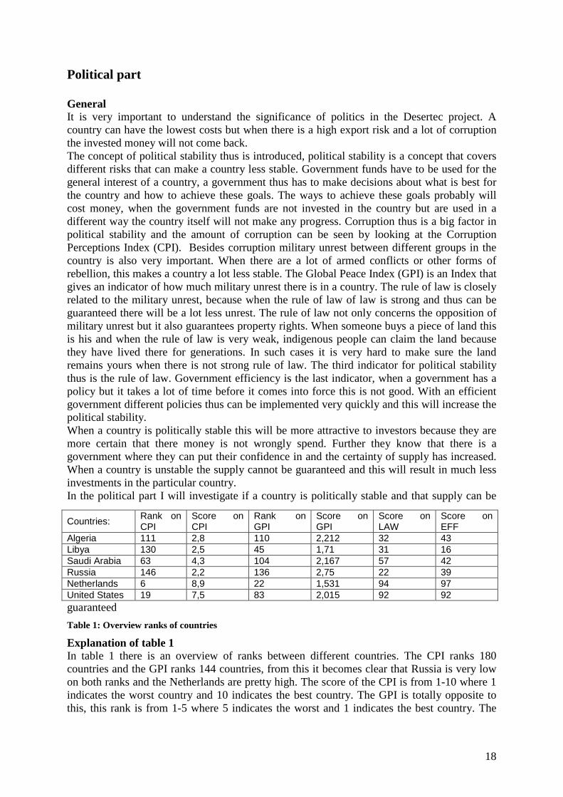
Political part General It is very important to understand the significance of politics in the Desertec project. A country can have the lowest costs but when there is a high export risk and a lot of corruption the invested money will not come back. The concept of political stability thus is introduced, political stability is a concept that covers different risks that can make a country less stable. Government funds have to be used for the general interest of a country, a government thus has to make decisions about what is best for the country and how to achieve these goals. The ways to achieve these goals probably will cost money, when the government funds are not invested in the country but are used in a different way the country itself will not make any progress. Corruption thus is a big factor in political stability and the amount of corruption can be seen by looking at the Corruption Perceptions Index (CPI). Besides corruption military unrest between different groups in the country is also very important. When there are a lot of armed conflicts or other forms of rebellion, this makes a country a lot less stable. The Global Peace Index (GPI) is an Index that gives an indicator of how much military unrest there is in a country. The rule of law is closely related to the military unrest, because when the rule of law of law is strong and thus can be guaranteed there will be a lot less unrest. The rule of law not only concerns the opposition of military unrest but it also guarantees property rights. When someone buys a piece of land this is his and when the rule of law is very weak, indigenous people can claim the land because they have lived there for generations. In such cases it is very hard to make sure the land remains yours when there is not strong rule of law. The third indicator for political stability thus is the rule of law. Government efficiency is the last indicator, when a government has a policy but it takes a lot of time before it comes into force this is not good. With an efficient government different policies thus can be implemented very quickly and this will increase the political stability. When a country is politically stable this will be more attractive to investors because they are more certain that there money is not wrongly spend. Further they know that there is a government where they can put their confidence in and the certainty of supply has increased. When a country is unstable the supply cannot be guaranteed and this will result in much less investments in the particular country. In the political part I will investigate if a country is politically stable and that supply can be

guaranteed

Table 1: Overview ranks of countries

Explanation of table 1 In table 1 there is an overview of ranks between different countries. The CPI ranks 180 countries and the GPI ranks 144 countries, from this it becomes clear that Russia is very low on both ranks and the Netherlands are pretty high. The score of the CPI is from 1-10 where 1 indicates the worst country and 10 indicates the best country. The GPI is totally opposite to this, this rank is from 1-5 where 5 indicates the worst and 1 indicates the best country. The

Countries: Rank on CPI

Score on CPI

Rank on GPI

Score on GPI

Score on LAW

Score on EFF

Algeria 111 2,8 110 2,212 32 43 Libya 130 2,5 45 1,71 31 16 Saudi Arabia 63 4,3 104 2,167 57 42 Russia 146 2,2 136 2,75 22 39 Netherlands 6 8,9 22 1,531 94 97 United States 19 7,5 83 2,015 92 92

19

score of LAW represents the rule of law and is from 1-100 where 100 is the best . EFF also is from 1-100 and here 100 is also the best and this indicates the efficiency of the government. Algeria Algeria is a democratic republic in North Africa, the country was a colony of France and is independent since 1962 [EVD Algeria, 2010]. After the declaration of independency there have been many problems with regards to the government of the country. Until 1989 there was a one party policy, there thus was a democracy but only party could be chosen and this resulted in a lot of opposition. In 1989 a system was introduced where more parties could be chosen, but this resulted in am armed conflict between different parties. Especially in the cities it has become a lot more peaceful but there are still many armed conflicts [EVD Algeria, 2010]. All this unrest in this country has led to a bad ranking on the Global Peace Index [GPI Algeria, 2009] which will make it a less attractive country to invest in. Due to all these conflicts there is less attention for all other problems that are present in the country. One such problem is corruption, Algeria is a country where there is a lot of corruption [CPI, 2009] and is hard to tackle. Corruption stays as prominent as it is because the big criminals are protected by a large amount of smaller criminals, this way the big criminals will not get arrested. Corruption is very bad for the politics of a country because many people are bribed by criminals and this way the decisions made are the decisions that are positive or at least not negative for these criminals. Algeria thus has a lot of corruption thus decisions made are affected by criminals. There is a risk in investing money in the government of Algeria because a big part of this money may be lost to corruption in the government. This is a reason for investors to invest in other regions then in Algeria. Corruption thus is very large but this is not the only part where the rule of law is ineffective. Property rights are also part of the law, when an investor buys a piece of land it is his by contract, but when property rights are not properly implemented in the system there will be a problem. Indigenous people will claim the land for themselves because their families lived there for centuries but the investor has bought this. The rule of law should make clear that the land is owned by the investor and thus is his. Algeria does not score very well [Kaufmann et all, 2006] on this subject. The rule of law thus is not very strong and property rights maybe can’t be ensured. The fourth pillar of political stability is the effectiveness of the government, does the policy implementation have to go through a lot of bureaucratic layers which results in a slow implementation, or does the policy implementation does not meet a lot of layers and is implemented very fast. Algeria does not score very well on the effectiveness scale [Kaufmann et all, 2006], this may be a result of the big role of corruption in the country and the fact that the rule of law can’t be guaranteed. Libya The political structure of Libya is unique, it is a dictatorship but in daily practise the decisions are made by the cabinet. They make the day to day decisions but if colonel Kadaffi does not agree with this he can stop every decision made. Colonel Kadaffi has the power after the coupe 1951, he has absolute power and stands above everyone in Libya. In his regime Kadaffi changed a lot in Libya and one of his first decisions was that all foreign firms should be privatized immediately and this also happened [EVD Libya, 2010]. This shows that Kadaffi does not want much foreign influence, which is influential in the Desertec project. There is not much conflict in the country, it has a pretty good ranking on the Global Peace Index [GPI Libya, 2009] and this may be a result of the dictatorship. Political parties are not allowed in Libya and the opposition groups are very ineffective and divided between each other [EVD Libya, 2010].

20

The government is big in Libya, Kadaffi has transformed the political structure of the country. He divided the country in1500 regions which all have a decentralised government [EVD Libya, 2010]. A lot of money is lost here due to corruption, because the regions have a decentralised government it is hard to control all the money. It is hard to control because the bureaucratic machine is enormous. Libya thus scores very badly on the Corruption Index [CPI, 2009]. The rule of law is a problem because everything is controlled by Kadaffi’s revolutionary committees. These are committees that act as political committees that have the power to control the press, the police, government institutions and the population itself [EVD Libya, 2010]. Therefore these are powerful committees but once again it is too large, it is not possible for the committees to check everything the police and the government does. They have to rely on them and because these institutions are corrupt the rule of law is hard to guarantee. The score of Libya also is not good for the rule of law [Kaufmann et all, 2006]. It is already mentioned but the bureaucracy is a very big problem in Libya, if you look to the central government it all looks pretty simple because there are not that many central ministries. But when the overall government is taken into account is all becomes very complicated because of the decentralized governments in the 1500 regions. The effectiveness of the government thus is very low [Kaufmann et all, 2006]. It takes a very long time until the policies are implemented in the different regions. Saudi Arabia Saudi Arabia is a monarchy where the crown stays in the bloodline of the Saudi family. The head of state therefore is not chosen by the people but the crown is passed on within the family. The council of Ministers is an institution that is chosen by the king and advises him on general policy and it also directs the activities of the bureaucratic machine. Legislation made by the Council of Ministers has been approved by the king and thus has to be implemented [Frontline, 2001]. Despite the clear rule of the king, there is much unrest in Saudi Arabia. The unrest is caused by religion and the monarchy. The main religion of Saudi Arabia is the Islam, but within the Islam there are all kinds of disparities, these have a lot of conflicts with each other. There thus is a lot of conflict between the different religions but there are also conflicts about the monarchy. There is also a lot of disagreement about who should be the head of state, because many people think that the monarchy is not good [Frontline, 2001]. In the end Saudi Arabia stands on a low rank in the Global Peace Index [GPI Saudi Arabia, 2009]. Corruption is not a very big problem because there is not a very large bureaucratic machine. Of course civil servants are needed, but it is far less extensive then in many other countries. The result is that the civil servants that are there can be controlled much better and therefore the corruption is not that high [CPI, 2009]. The rule of law in Saudi Arabia is determined by religion, they follow the Sharia which is the law stated in the Koran. This law is pretty strict and the punishments are very old fashioned. There are many corporal punishments still legal in Saudi Arabia. The rule of law also gets a good rank [Kaufmann et all, 2006], property rights thus can be guaranteed with quite some certainty. Is previously mentioned the bureaucratic machine is not that big which makes it easier to govern. The effectiveness of the government thus increases because of the smaller bureaucracy. Important decisions are also made faster because the king is the only one who can make this decision. The king is advised by the council of ministers but in the end he will make a decision and everybody has to agree with this. On the other side the king always makes his own decision, maybe the decision made is what he thinks is best but in the end will prove to be a lot less efficient. Government efficiency thus is not bad [Kaufmann et all, 2006].

21

5. Scenarios For the elaboration of the scenarios we will use the model and the data as presented in chapter 3 and 4. In this chapter there are four scenarios that are put in the model. The scenarios will be described first and then there are 6 graphs, where the results are presented. The six graphs describe the total costs, total emissions and the market price of CSP. After these three graphs there are three graphs with the quantities of coal, gas and CSP produced. The outputs in the six graphs are al calculated with a discount rate. Except for total costs, these are also calculated without a discount rate. The scenarios will be presented in the following order:

� Emissions o Basic scenario with no restrictions on emissions o Scenario with prices on emissions. o Quantity restriction on emissions.

� European demand o Basic scenario where the three countries do not have to supply to Europe. o Scenario where the three countries have to supply 25% of total European

demand. o Scenario where the three countries have to supply 40% of total European

demand. � Political scenario

o Basic scenario without any political influence. o Scenario with moderate political influence. o Scenario with high political influence.

� Prices gas and coal o Basic scenario where prices of gas and coal are equal to the 2000 level. o Scenario where prices increase as forecasts predict. o Scenario where prices increase at an extreme rate.

22

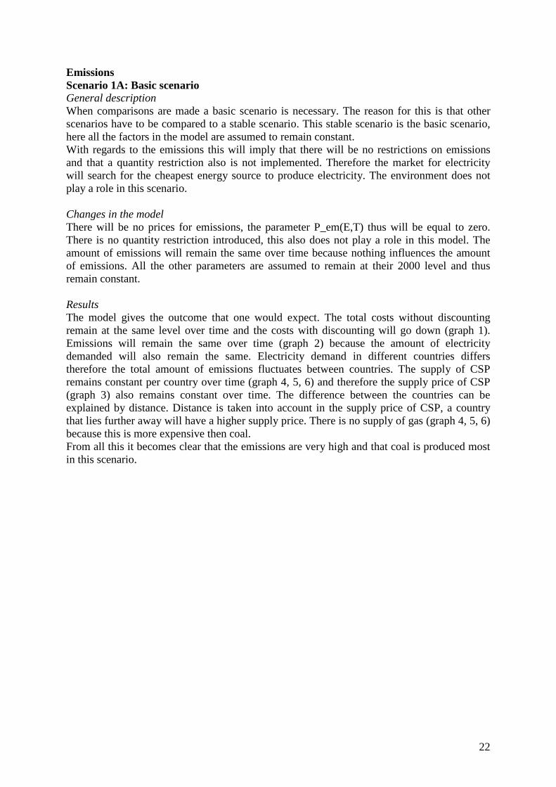
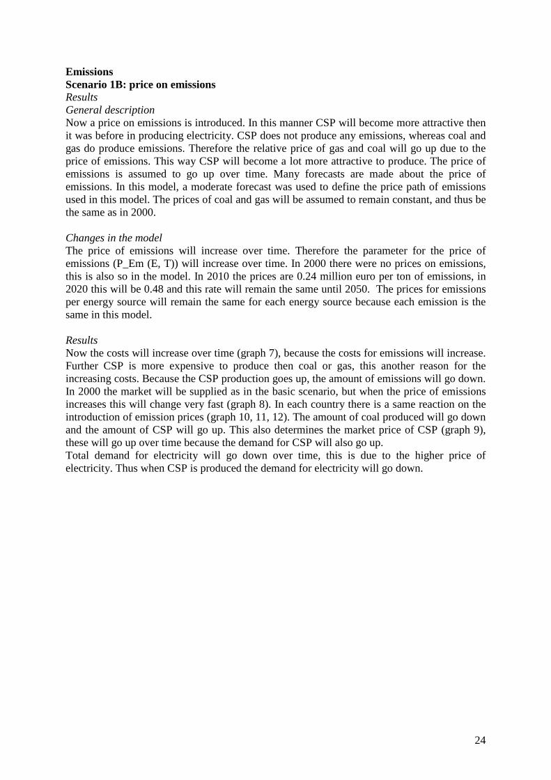
Emissions Scenario 1A: Basic scenario General description When comparisons are made a basic scenario is necessary. The reason for this is that other scenarios have to be compared to a stable scenario. This stable scenario is the basic scenario, here all the factors in the model are assumed to remain constant. With regards to the emissions this will imply that there will be no restrictions on emissions and that a quantity restriction also is not implemented. Therefore the market for electricity will search for the cheapest energy source to produce electricity. The environment does not play a role in this scenario. Changes in the model There will be no prices for emissions, the parameter P_em(E,T) thus will be equal to zero. There is no quantity restriction introduced, this also does not play a role in this model. The amount of emissions will remain the same over time because nothing influences the amount of emissions. All the other parameters are assumed to remain at their 2000 level and thus remain constant. Results The model gives the outcome that one would expect. The total costs without discounting remain at the same level over time and the costs with discounting will go down (graph 1). Emissions will remain the same over time (graph 2) because the amount of electricity demanded will also remain the same. Electricity demand in different countries differs therefore the total amount of emissions fluctuates between countries. The supply of CSP remains constant per country over time (graph 4, 5, 6) and therefore the supply price of CSP (graph 3) also remains constant over time. The difference between the countries can be explained by distance. Distance is taken into account in the supply price of CSP, a country that lies further away will have a higher supply price. There is no supply of gas (graph 4, 5, 6) because this is more expensive then coal. From all this it becomes clear that the emissions are very high and that coal is produced most in this scenario.

23

Graph 1: total costs over time

0,000

20000,000

40000,000

60000,000

80000,000

100000,000

120000,000

2000 2010 2020 2030 2040 2050

Time

tota

l co

sts

(mln

$)

with discounting without discounting

Graph 3: market price of CSP

270 275 280 285 290

2000

2010

2020

2030

2040

2050

Tim

e

market price of CSP (mln$/GW)

Algeria Libya Saudi Arabia

Graph 2: Total amount of emissions

2500 2600 2700 2800 2900 3000

2000

2010

2020

2030

2040

2050

tim

e

amount of emissions


Graph 4: amount of energy produced in Algeria

0 100 200 300 400 500 600

2000

2010

2020

2030

2040

2050ti

me

Amount produced in tons

Amount of gas produced Amount of coal produced

amount of CSP produced

Graph 6: Amount of energy produced in Suadi Arabia

0 100 200 300 400 500 600

2000

2010

2020

2030

2040

2050

tim

e


Amount of gas prodcued Amount of coal produced

Amount of CSP produced

Graph 5: Amount of energy produced in Libya

0 100 200 300 400 500 600

2000

2010

2020

2030

2040

2050

Tim

e




24

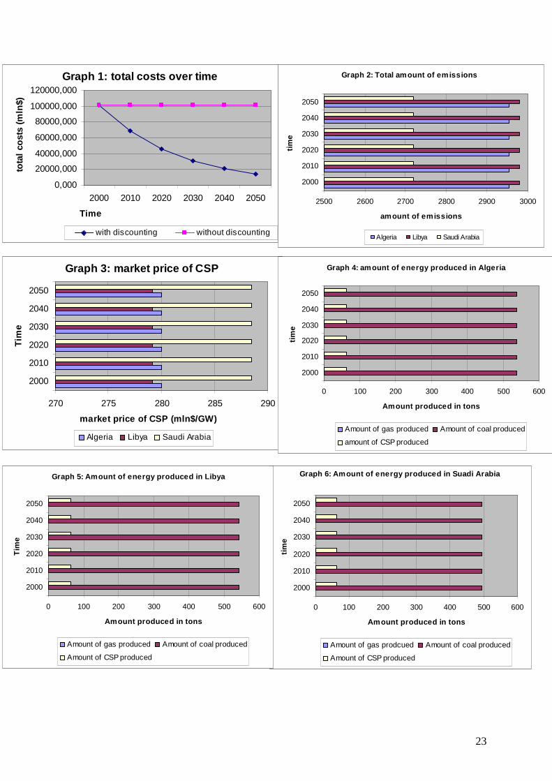
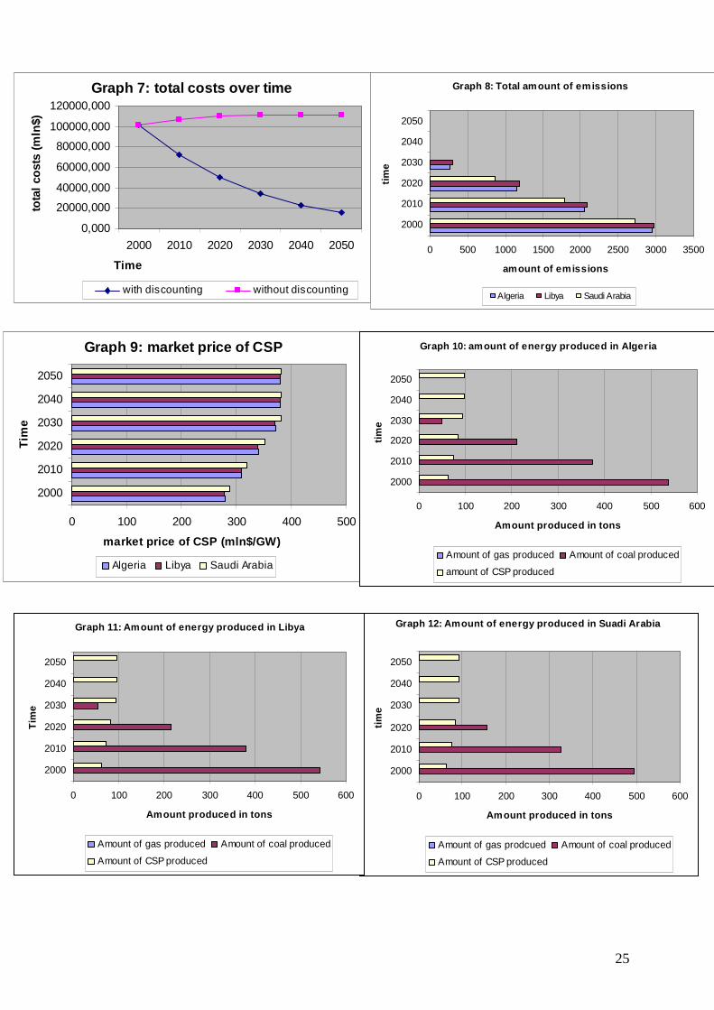
Emissions Scenario 1B: price on emissions Results General description Now a price on emissions is introduced. In this manner CSP will become more attractive then it was before in producing electricity. CSP does not produce any emissions, whereas coal and gas do produce emissions. Therefore the relative price of gas and coal will go up due to the price of emissions. This way CSP will become a lot more attractive to produce. The price of emissions is assumed to go up over time. Many forecasts are made about the price of emissions. In this model, a moderate forecast was used to define the price path of emissions used in this model. The prices of coal and gas will be assumed to remain constant, and thus be the same as in 2000. Changes in the model The price of emissions will increase over time. Therefore the parameter for the price of emissions (P_Em (E, T)) will increase over time. In 2000 there were no prices on emissions, this is also so in the model. In 2010 the prices are 0.24 million euro per ton of emissions, in 2020 this will be 0.48 and this rate will remain the same until 2050. The prices for emissions per energy source will remain the same for each energy source because each emission is the same in this model. Results Now the costs will increase over time (graph 7), because the costs for emissions will increase. Further CSP is more expensive to produce then coal or gas, this another reason for the increasing costs. Because the CSP production goes up, the amount of emissions will go down. In 2000 the market will be supplied as in the basic scenario, but when the price of emissions increases this will change very fast (graph 8). In each country there is a same reaction on the introduction of emission prices (graph 10, 11, 12). The amount of coal produced will go down and the amount of CSP will go up. This also determines the market price of CSP (graph 9), these will go up over time because the demand for CSP will also go up. Total demand for electricity will go down over time, this is due to the higher price of electricity. Thus when CSP is produced the demand for electricity will go down.

25


0,000

20000,000

40000,000

60000,000

80000,000

100000,000

120000,000

2000 2010 2020 2030 2040 2050

Time

tota

l co

sts

(mln

$)



0 100 200 300 400 500

2000

2010

2020

2030

2040

2050

Tim

e




0 100 200 300 400 500 600

2000

2010

2020

2030

2040

2050ti

me





0 100 200 300 400 500 600

2000

2010

2020

2030

2040

2050

tim

e





0 100 200 300 400 500 600

2000

2010

2020

2030

2040

2050

Tim

e





0 500 1000 1500 2000 2500 3000 3500

2000

2010

2020

2030

2040

2050

tim

e

amount of emissions


26

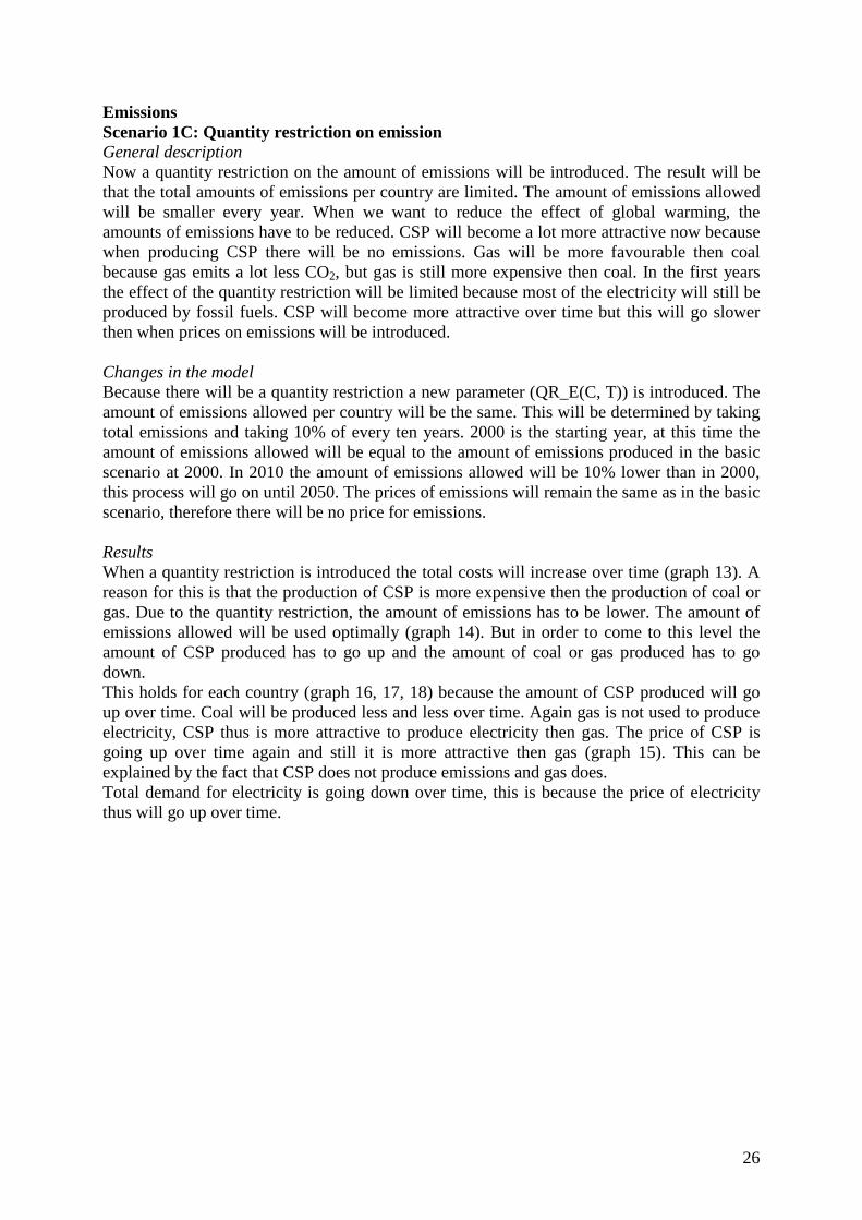
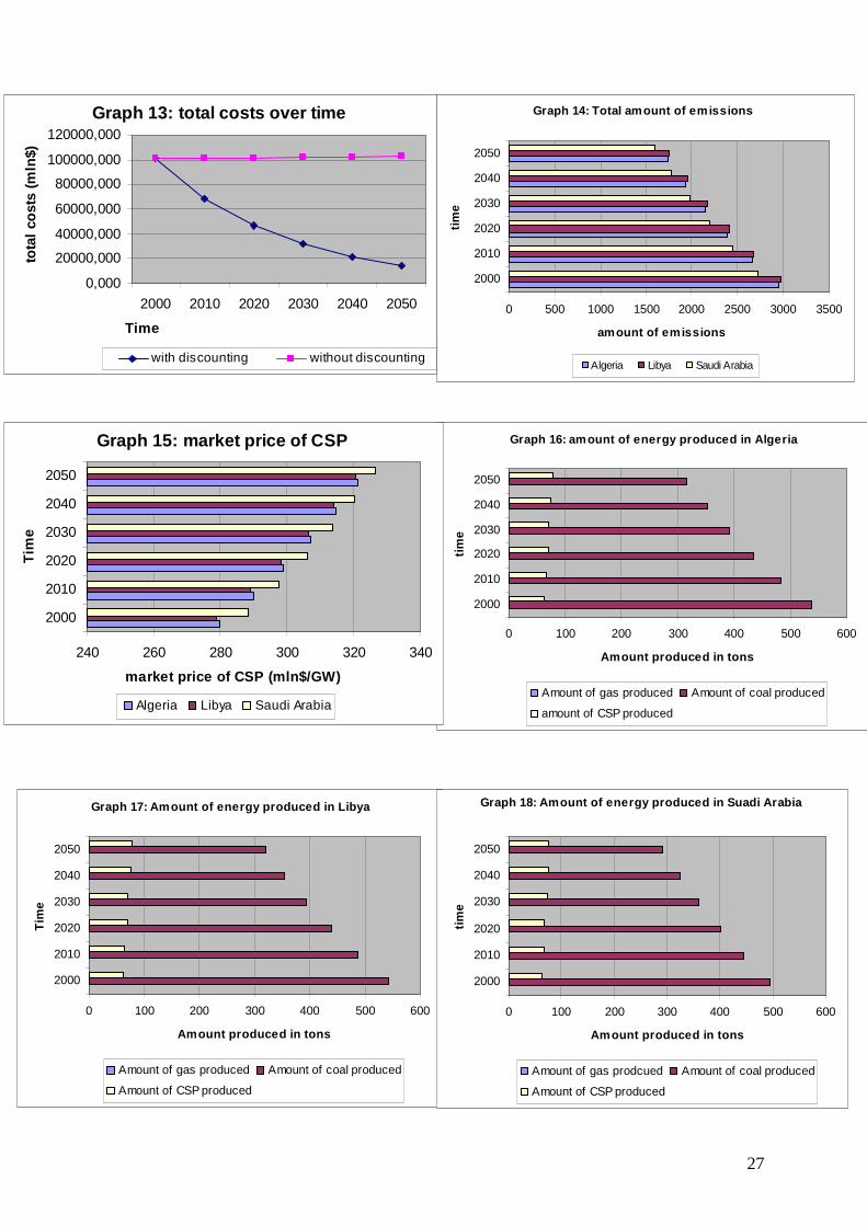
Emissions Scenario 1C: Quantity restriction on emission General description Now a quantity restriction on the amount of emissions will be introduced. The result will be that the total amounts of emissions per country are limited. The amount of emissions allowed will be smaller every year. When we want to reduce the effect of global warming, the amounts of emissions have to be reduced. CSP will become a lot more attractive now because when producing CSP there will be no emissions. Gas will be more favourable then coal because gas emits a lot less CO2, but gas is still more expensive then coal. In the first years the effect of the quantity restriction will be limited because most of the electricity will still be produced by fossil fuels. CSP will become more attractive over time but this will go slower then when prices on emissions will be introduced. Changes in the model Because there will be a quantity restriction a new parameter (QR_E(C, T)) is introduced. The amount of emissions allowed per country will be the same. This will be determined by taking total emissions and taking 10% of every ten years. 2000 is the starting year, at this time the amount of emissions allowed will be equal to the amount of emissions produced in the basic scenario at 2000. In 2010 the amount of emissions allowed will be 10% lower than in 2000, this process will go on until 2050. The prices of emissions will remain the same as in the basic scenario, therefore there will be no price for emissions. Results When a quantity restriction is introduced the total costs will increase over time (graph 13). A reason for this is that the production of CSP is more expensive then the production of coal or gas. Due to the quantity restriction, the amount of emissions has to be lower. The amount of emissions allowed will be used optimally (graph 14). But in order to come to this level the amount of CSP produced has to go up and the amount of coal or gas produced has to go down. This holds for each country (graph 16, 17, 18) because the amount of CSP produced will go up over time. Coal will be produced less and less over time. Again gas is not used to produce electricity, CSP thus is more attractive to produce electricity then gas. The price of CSP is going up over time again and still it is more attractive then gas (graph 15). This can be explained by the fact that CSP does not produce emissions and gas does. Total demand for electricity is going down over time, this is because the price of electricity thus will go up over time.

27


0 500 1000 1500 2000 2500 3000 3500

2000

2010

2020

2030

2040

2050

tim

e

amount of emissions



0,000

20000,000

40000,000

60000,000

80000,000

100000,000

120000,000

2000 2010 2020 2030 2040 2050

Time

tota

l co

sts

(mln

$)



0 100 200 300 400 500 600

2000

2010

2020

2030

2040

2050

tim

e





0 100 200 300 400 500 600

2000

2010

2020

2030

2040

2050

Tim

e





0 100 200 300 400 500 600

2000

2010

2020

2030

2040

2050

tim

e





240 260 280 300 320 340

2000

2010

2020

2030

2040

2050

Tim

e



28

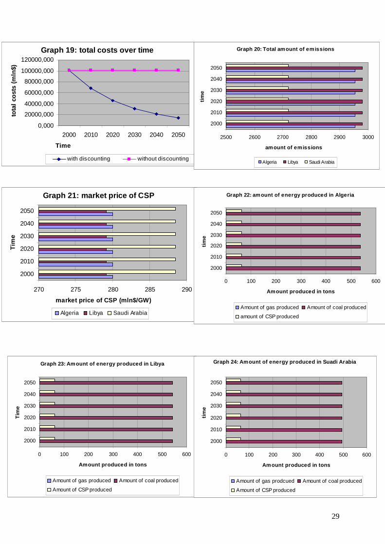
European Demand Scenario 2A: Basic scenario of European demand General description In this thesis the Desertec project is an important source of inspiration. The Desertec project looks at the possibility of producing electricity with solar panels in deserts and transporting this electricity to other regions. In this thesis the three countries investigated will try to produce electricity for the European market. The European electricity market is a huge market and it is possible to produce electricity with CSP and then transport this to Europe. But CSP is not the only energy source with which these countries can produce electricity. The demand for electricity therefore can be satisfied by fossil fuels or CSP. In the basic model the European demand does not yet have any influence, countries do not have to supply part of the electricity needed in Europe Changes in the model In this scenario there is not yet any minimum demand in Europe that has to be met. But we already introduce new parameters here. The first parameter is total European demand (Eur_D(C)) for each country. The second parameter (EUR_P(C)) describes the fraction of the electricity market that has to be supplied by the three countries. Besides the new parameters, a new equation is introduced also. This equation (eDemE(C)) represents the total demand for electricity in Europe that has to be met in this model. With this equation a variable (vT_DE(C)) is calculated and this thus represents the total electricity demand from Europe that has to be met in this model. This variable is added to the right side of the equation of the total demand for electricity that has to be met (eDemandGW(C)). Results The results are the same as in the basic model of emissions. This is so because the fraction of European demand that has to be met now equals zero, total demand thus will not increase. The outcome thus will be the same as in the basic scenario of emission. The total costs will remain the same over time (graph 19), and the total emissions will remain at a high stable level (graph 20). The amount of coal produced will be very high (graph 22, 23, 24). CSP will also be produced but at a much lower level (graph 22, 23, 24). The price of CSP will also remain the same over time (graph 21). Overall the amount of emissions will be very high and most electricity will be produced by coal.

29


0,000

20000,000

40000,000

60000,000

80000,000

100000,000

120000,000

2000 2010 2020 2030 2040 2050

Time

tota

l co

sts

(mln

$)



270 275 280 285 290

2000

2010

2020

2030

2040

2050

Tim

e




2500 2600 2700 2800 2900 3000

2000

2010

2020

2030

2040

2050

tim

e

amount of emissions



0 100 200 300 400 500 600

2000

2010

2020

2030

2040

2050

Tim

e





0 100 200 300 400 500 600

2000

2010

2020

2030

2040

2050

tim

e





0 100 200 300 400 500 600

2000

2010

2020

2030

2040

2050

tim

e




30

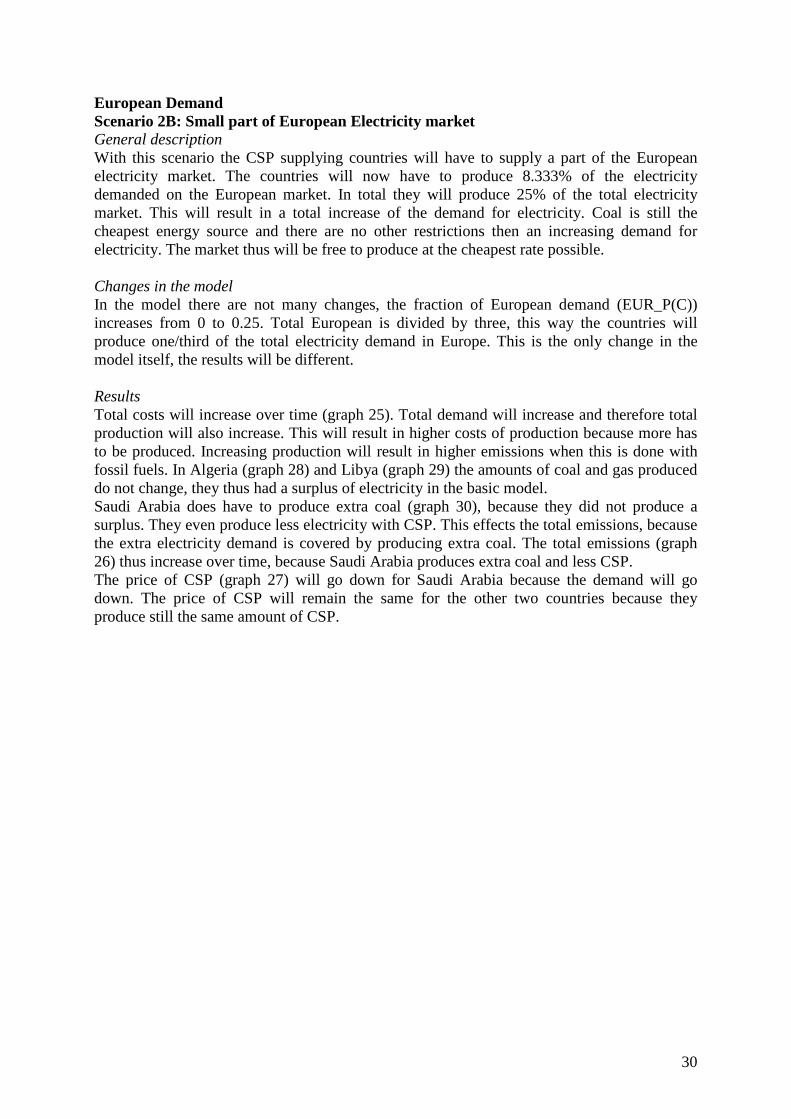
European Demand Scenario 2B: Small part of European Electricity market General description With this scenario the CSP supplying countries will have to supply a part of the European electricity market. The countries will now have to produce 8.333% of the electricity demanded on the European market. In total they will produce 25% of the total electricity market. This will result in a total increase of the demand for electricity. Coal is still the cheapest energy source and there are no other restrictions then an increasing demand for electricity. The market thus will be free to produce at the cheapest rate possible. Changes in the model In the model there are not many changes, the fraction of European demand (EUR_P(C)) increases from 0 to 0.25. Total European is divided by three, this way the countries will produce one/third of the total electricity demand in Europe. This is the only change in the model itself, the results will be different. Results Total costs will increase over time (graph 25). Total demand will increase and therefore total production will also increase. This will result in higher costs of production because more has to be produced. Increasing production will result in higher emissions when this is done with fossil fuels. In Algeria (graph 28) and Libya (graph 29) the amounts of coal and gas produced do not change, they thus had a surplus of electricity in the basic model. Saudi Arabia does have to produce extra coal (graph 30), because they did not produce a surplus. They even produce less electricity with CSP. This effects the total emissions, because the extra electricity demand is covered by producing extra coal. The total emissions (graph 26) thus increase over time, because Saudi Arabia produces extra coal and less CSP. The price of CSP (graph 27) will go down for Saudi Arabia because the demand will go down. The price of CSP will remain the same for the other two countries because they produce still the same amount of CSP.

31


0,000

20000,000

40000,000

60000,000

80000,000

100000,000

120000,000

2000 2010 2020 2030 2040 2050

Time

tota

l co

sts

(mln

$)



230 240 250 260 270 280 290

2000

2010

2020

2030

2040

2050

Tim

e




0 1000 2000 3000 4000 5000

2000

2010

2020

2030

2040

2050

tim

e

amount of emissions



0 100 200 300 400 500 600

2000

2010

2020

2030

2040

2050ti

me





0 200 400 600 800

2000

2010

2020

2030

2040

2050

tim

e





0 100 200 300 400 500 600

2000

2010

2020

2030

2040

2050

Tim

e




32

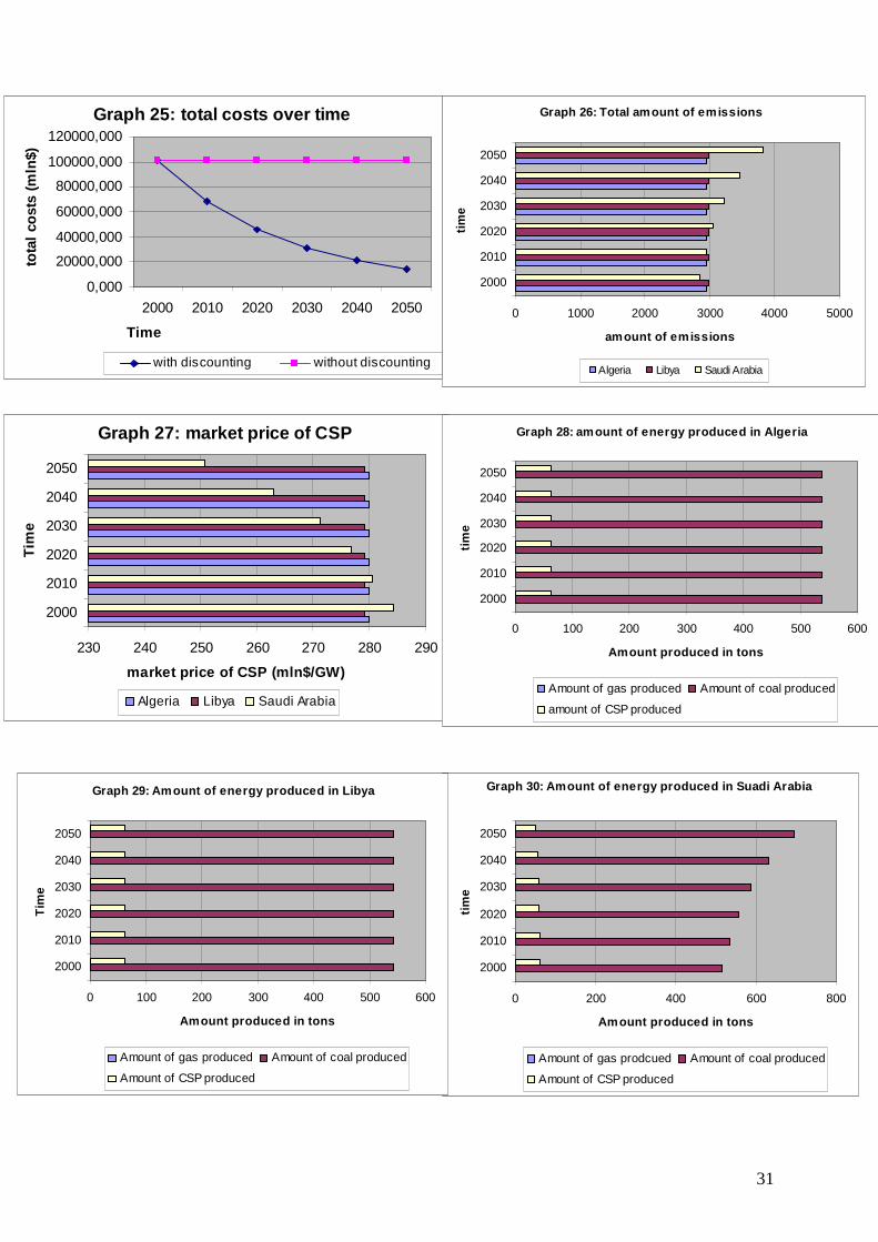
European Demand Scenario 2C: Bigger part of European Electricity market General description In this scenario the CSP supplying countries will have to produce an even larger part of the European electricity market. Now each country has to supply 13.333% of the total European electricity market. In total the CSP supplying countries will now produce 40% of the total European demand. Again coal is the cheapest option. Because there are no other restrictions the extra demand will probably be satisfied by coal. Changes in the model In the model there are not many changes, the fraction of European demand (EUR_P(C)) increases from 0 to 0.4. Total European demand is divided by three, this way each country will produce one/third of total electricity demand. This is the only change in the model itself, the results will be different. Results As compared to the moderate scenario the costs now increase much more (graph 31). This can be explained by looking at the quantities produced of each energy source for each country. Saudi Arabia already had to produce more coal in the moderate scenario (graph 36), but now it has to produce much more coal. The amount of CSP produced is going down over time. Algeria (graph 34) and Libya (graph 35) are now also producing extra coal to try to meet the extra electricity demand. These countries also produce less CSP over time. Total costs will increase because every country just has to produce a lot more. Total emissions also rise very fast (graph 32), because of high coal production and low CSP production the total emissions rise very fast. The price of CSP price also goes down (graph 33), this is due to the lower demand for CSP.

33


0,000

20000,000

40000,000

60000,000

80000,000

100000,000

120000,000

2000 2010 2020 2030 2040 2050

Time

tota

l co

sts

(mln

$)



0 50 100 150 200 250 300

2000

2010

2020

2030

2040

2050

Tim

e




0 200 400 600 800 1000

2000

2010

2020

2030

2040

2050

Tim

e





0 500 1000 1500

2000

2010

2020

2030

2040

2050

tim

e





0 2000 4000 6000 8000 10000

2000

2010

2020

2030

2040

2050

tim

e

amount of emissions



0 200 400 600 800 1000

2000

2010

2020

2030

2040

2050ti

me




34

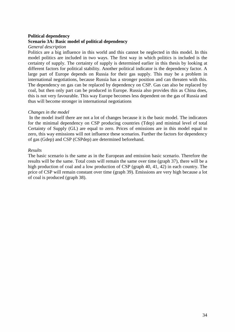
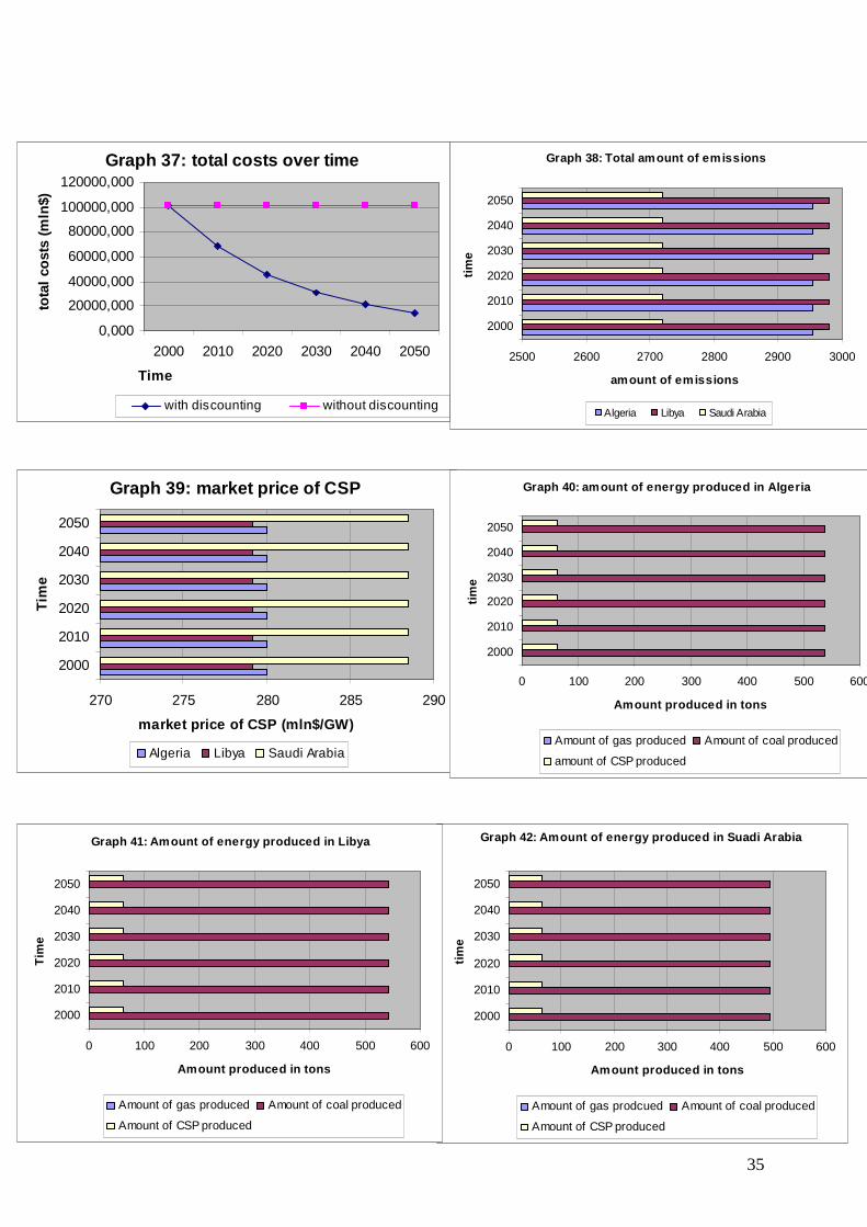
Political dependency Scenario 3A: Basic model of political dependency General description Politics are a big influence in this world and this cannot be neglected in this model. In this model politics are included in two ways. The first way in which politics is included is the certainty of supply. The certainty of supply is determined earlier in this thesis by looking at different factors for political stability. Another political indicator is the dependency factor. A large part of Europe depends on Russia for their gas supply. This may be a problem in international negotiations, because Russia has a stronger position and can threaten with this. The dependency on gas can be replaced by dependency on CSP. Gas can also be replaced by coal, but then only part can be produced in Europe. Russia also provides this as China does, this is not very favourable. This way Europe becomes less dependent on the gas of Russia and thus will become stronger in international negotiations Changes in the model In the model itself there are not a lot of changes because it is the basic model. The indicators for the minimal dependency on CSP producing countries (Tdep) and minimal level of total Certainty of Supply (GL) are equal to zero. Prices of emissions are in this model equal to zero, this way emissions will not influence these scenarios. Further the factors for dependency of gas (Gdep) and CSP (CSPdep) are determined beforehand. Results The basic scenario is the same as in the European and emission basic scenario. Therefore the results will be the same. Total costs will remain the same over time (graph 37), there will be a high production of coal and a low production of CSP (graph 40, 41, 42) in each country. The price of CSP will remain constant over time (graph 39). Emissions are very high because a lot of coal is produced (graph 38).

35


0 100 200 300 400 500 600

2000

2010

2020

2030

2040

2050

tim

e





0 100 200 300 400 500 600

2000

2010

2020

2030

2040

2050

Tim

e





270 275 280 285 290

2000

2010

2020

2030

2040

2050

Tim

e




0 100 200 300 400 500 600

2000

2010

2020

2030

2040

2050

tim

e





2500 2600 2700 2800 2900 3000

2000

2010

2020

2030

2040

2050

tim

e

amount of emissions



0,000

20000,000

40000,000

60000,000

80000,000

100000,000

120000,000

2000 2010 2020 2030 2040 2050

Time

tota

l co

sts

(mln

$)


36

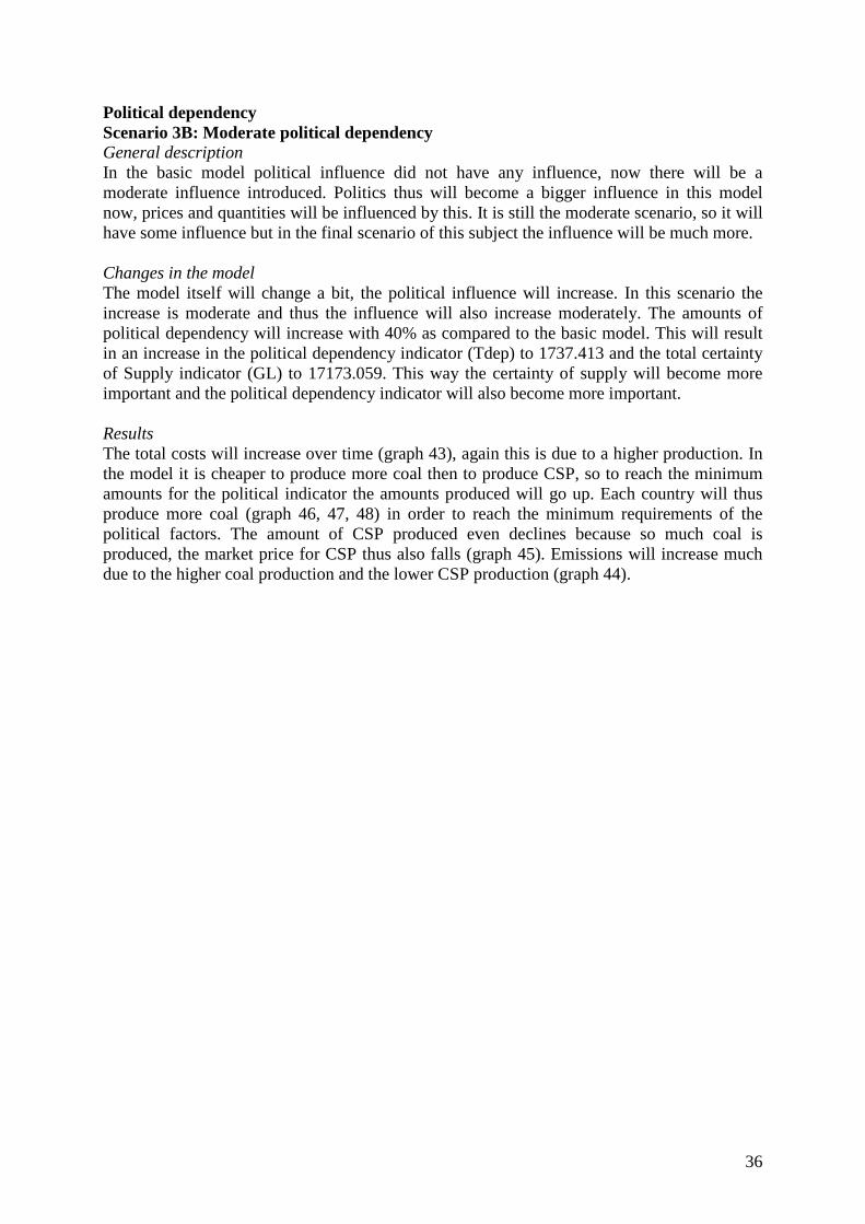
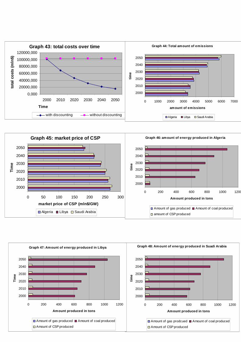
Political dependency Scenario 3B: Moderate political dependency General description In the basic model political influence did not have any influence, now there will be a moderate influence introduced. Politics thus will become a bigger influence in this model now, prices and quantities will be influenced by this. It is still the moderate scenario, so it will have some influence but in the final scenario of this subject the influence will be much more. Changes in the model The model itself will change a bit, the political influence will increase. In this scenario the increase is moderate and thus the influence will also increase moderately. The amounts of political dependency will increase with 40% as compared to the basic model. This will result in an increase in the political dependency indicator (Tdep) to 1737.413 and the total certainty of Supply indicator (GL) to 17173.059. This way the certainty of supply will become more important and the political dependency indicator will also become more important. Results The total costs will increase over time (graph 43), again this is due to a higher production. In the model it is cheaper to produce more coal then to produce CSP, so to reach the minimum amounts for the political indicator the amounts produced will go up. Each country will thus produce more coal (graph 46, 47, 48) in order to reach the minimum requirements of the political factors. The amount of CSP produced even declines because so much coal is produced, the market price for CSP thus also falls (graph 45). Emissions will increase much due to the higher coal production and the lower CSP production (graph 44).

37


0,000

20000,000

40000,000

60000,000

80000,000

100000,000

120000,000

2000 2010 2020 2030 2040 2050

Time

tota

l co

sts

(mln

$)



0 50 100 150 200 250 300

2000

2010

2020

2030

2040

2050

Tim

e




0 1000 2000 3000 4000 5000 6000 7000

2000

2010

2020

2030

2040

2050

tim

e

amount of emissions



0 200 400 600 800 1000 1200

2000

2010

2020

2030

2040

2050

tim

e





0 200 400 600 800 1000 1200

2000

2010

2020

2030

2040

2050

tim

e





0 200 400 600 800 1000 1200

2000

2010

2020

2030

2040

2050

Tim

e




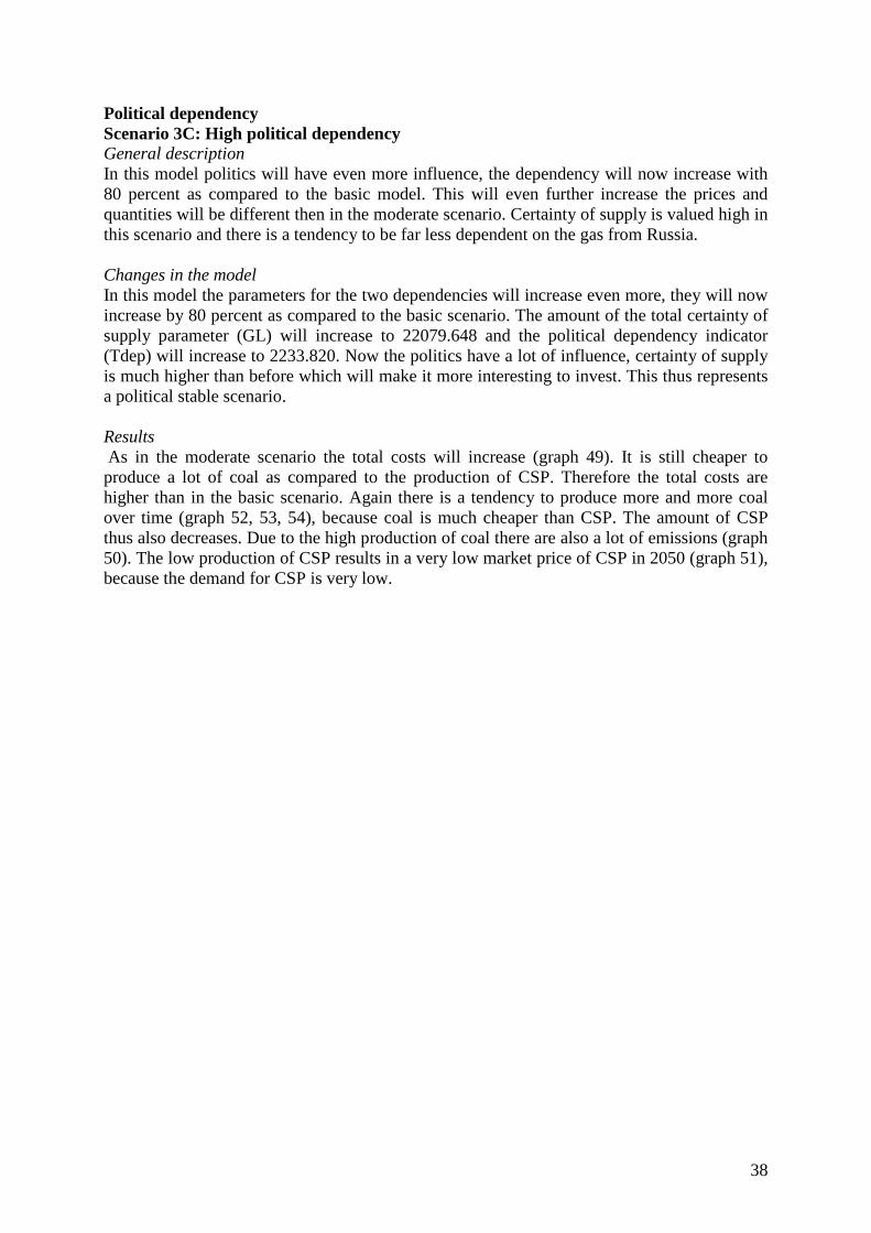
38

Political dependency Scenario 3C: High political dependency General description In this model politics will have even more influence, the dependency will now increase with 80 percent as compared to the basic model. This will even further increase the prices and quantities will be different then in the moderate scenario. Certainty of supply is valued high in this scenario and there is a tendency to be far less dependent on the gas from Russia. Changes in the model In this model the parameters for the two dependencies will increase even more, they will now increase by 80 percent as compared to the basic scenario. The amount of the total certainty of supply parameter (GL) will increase to 22079.648 and the political dependency indicator (Tdep) will increase to 2233.820. Now the politics have a lot of influence, certainty of supply is much higher than before which will make it more interesting to invest. This thus represents a political stable scenario. Results As in the moderate scenario the total costs will increase (graph 49). It is still cheaper to produce a lot of coal as compared to the production of CSP. Therefore the total costs are higher than in the basic scenario. Again there is a tendency to produce more and more coal over time (graph 52, 53, 54), because coal is much cheaper than CSP. The amount of CSP thus also decreases. Due to the high production of coal there are also a lot of emissions (graph 50). The low production of CSP results in a very low market price of CSP in 2050 (graph 51), because the demand for CSP is very low.

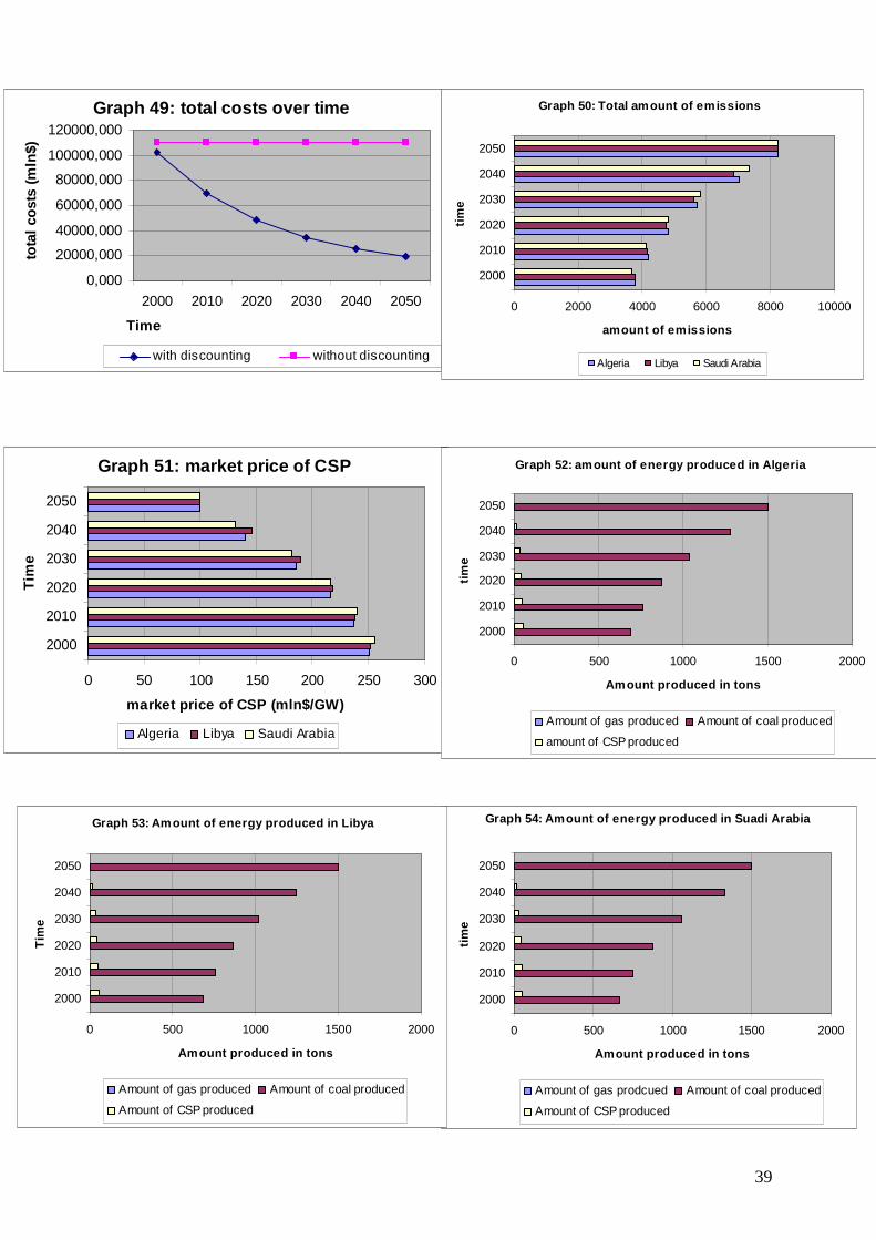
39


0 500 1000 1500 2000

2000

2010

2020

2030

2040

2050

tim

e





0 500 1000 1500 2000

2000

2010

2020

2030

2040

2050

Tim

e





0 50 100 150 200 250 300

2000

2010

2020

2030

2040

2050

Tim

e




0 500 1000 1500 2000

2000

2010

2020

2030

2040

2050

tim

e





0,000

20000,000

40000,000

60000,000

80000,000

100000,000

120000,000

2000 2010 2020 2030 2040 2050

Time

tota

l co

sts

(mln

$)



0 2000 4000 6000 8000 10000

2000

2010

2020

2030

2040

2050

tim

e

amount of emissions


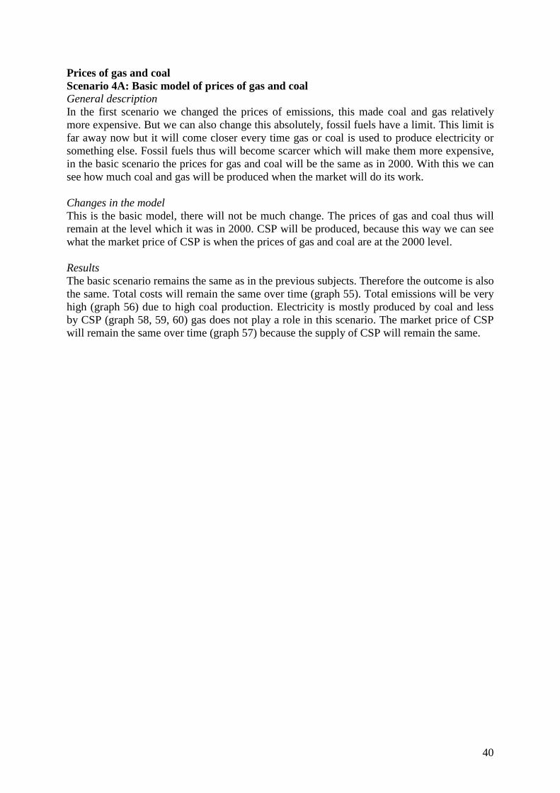
40

Prices of gas and coal Scenario 4A: Basic model of prices of gas and coal General description In the first scenario we changed the prices of emissions, this made coal and gas relatively more expensive. But we can also change this absolutely, fossil fuels have a limit. This limit is far away now but it will come closer every time gas or coal is used to produce electricity or something else. Fossil fuels thus will become scarcer which will make them more expensive, in the basic scenario the prices for gas and coal will be the same as in 2000. With this we can see how much coal and gas will be produced when the market will do its work. Changes in the model This is the basic model, there will not be much change. The prices of gas and coal thus will remain at the level which it was in 2000. CSP will be produced, because this way we can see what the market price of CSP is when the prices of gas and coal are at the 2000 level. Results The basic scenario remains the same as in the previous subjects. Therefore the outcome is also the same. Total costs will remain the same over time (graph 55). Total emissions will be very high (graph 56) due to high coal production. Electricity is mostly produced by coal and less by CSP (graph 58, 59, 60) gas does not play a role in this scenario. The market price of CSP will remain the same over time (graph 57) because the supply of CSP will remain the same.

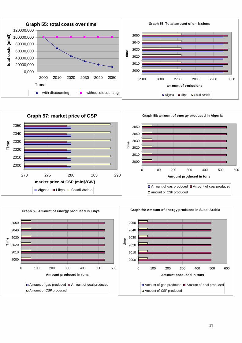
41


0 100 200 300 400 500 600

2000

2010

2020

2030

2040

2050

tim

e





0 100 200 300 400 500 600

2000

2010

2020

2030

2040

2050

Tim

e





270 275 280 285 290

2000

2010

2020

2030

2040

2050

Tim

e




0 100 200 300 400 500 600

2000

2010

2020

2030

2040

2050ti

me





2500 2600 2700 2800 2900 3000

2000

2010

2020

2030

2040

2050

tim

e

amount of emissions



0,000

20000,000

40000,000

60000,000

80000,000

100000,000

120000,000

2000 2010 2020 2030 2040 2050

Time

tota

l co

sts

(mln

$)


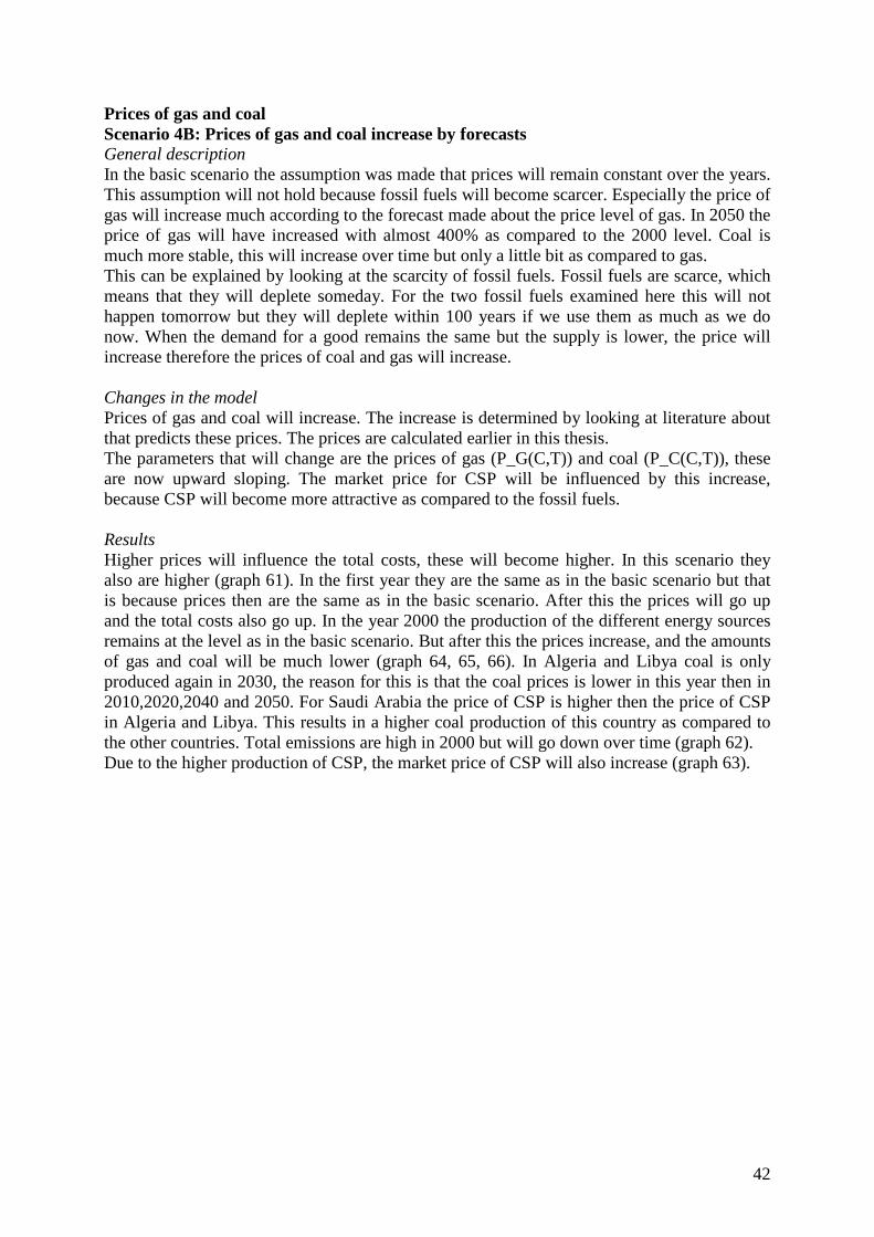
42

Prices of gas and coal Scenario 4B: Prices of gas and coal increase by forecasts General description In the basic scenario the assumption was made that prices will remain constant over the years. This assumption will not hold because fossil fuels will become scarcer. Especially the price of gas will increase much according to the forecast made about the price level of gas. In 2050 the price of gas will have increased with almost 400% as compared to the 2000 level. Coal is much more stable, this will increase over time but only a little bit as compared to gas. This can be explained by looking at the scarcity of fossil fuels. Fossil fuels are scarce, which means that they will deplete someday. For the two fossil fuels examined here this will not happen tomorrow but they will deplete within 100 years if we use them as much as we do now. When the demand for a good remains the same but the supply is lower, the price will increase therefore the prices of coal and gas will increase. Changes in the model Prices of gas and coal will increase. The increase is determined by looking at literature about that predicts these prices. The prices are calculated earlier in this thesis. The parameters that will change are the prices of gas (P_G(C,T)) and coal (P_C(C,T)), these are now upward sloping. The market price for CSP will be influenced by this increase, because CSP will become more attractive as compared to the fossil fuels. Results Higher prices will influence the total costs, these will become higher. In this scenario they also are higher (graph 61). In the first year they are the same as in the basic scenario but that is because prices then are the same as in the basic scenario. After this the prices will go up and the total costs also go up. In the year 2000 the production of the different energy sources remains at the level as in the basic scenario. But after this the prices increase, and the amounts of gas and coal will be much lower (graph 64, 65, 66). In Algeria and Libya coal is only produced again in 2030, the reason for this is that the coal prices is lower in this year then in 2010,2020,2040 and 2050. For Saudi Arabia the price of CSP is higher then the price of CSP in Algeria and Libya. This results in a higher coal production of this country as compared to the other countries. Total emissions are high in 2000 but will go down over time (graph 62). Due to the higher production of CSP, the market price of CSP will also increase (graph 63).

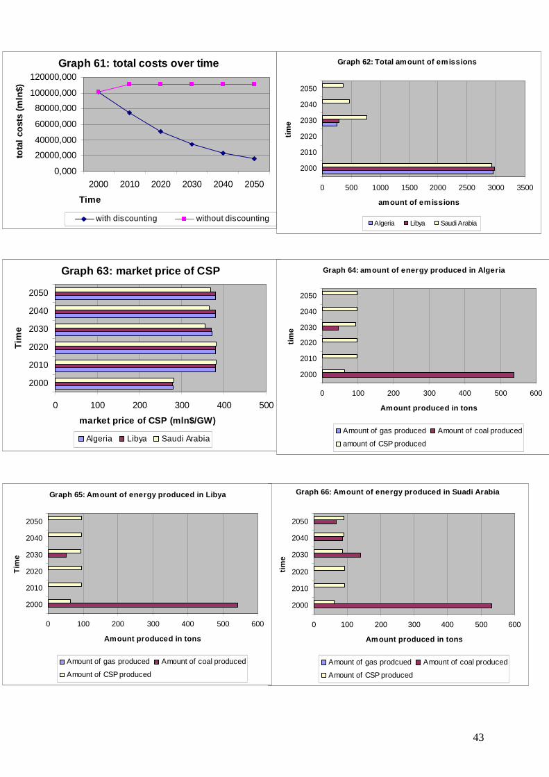
43


0 100 200 300 400 500 600

2000

2010

2020

2030

2040

2050

tim

e





0 100 200 300 400 500 600

2000

2010

2020

2030

2040

2050

Tim

e





0 100 200 300 400 500

2000

2010

2020

2030

2040

2050

Tim

e




0 100 200 300 400 500 600

2000

2010

2020

2030

2040

2050ti

me





0 500 1000 1500 2000 2500 3000 3500

2000

2010

2020

2030

2040

2050

tim

e

amount of emissions



0,000

20000,000

40000,000

60000,000

80000,000

100000,000

120000,000

2000 2010 2020 2030 2040 2050

Time

tota

l co

sts

(mln

$)


44

Prices of gas and coal Scenario 4C: Prices of gas and coal extreme increase General description In the previous scenario the forecasts were made on the basis of the market. The prices increased and this resulted in the previous scenario. Now the prices will increase much more then in the previous scenario. The difference between one year and the next will be multiplied by two, this way the prices will increase two times as fast. This scenario describes an extreme case, where fossil fuels will deplete much faster then expected and thus the price will increase much faster then expected. Changes in the model Again the prices of gas and coal will increase, but now the difference between two years is multiplied by two. The difference for the price of gas between 2000 and 2010 is the price of gas in 2010-price of gas in 2000, then this is multiplied by two and added to the price of 2000. Now we have the new price in 2010, the same thing is done for 2020. Price of gas in 2020-price of gas in 2000, this difference is multiplied by two and then added to the price of gas in 2000. This is done for all the prices for gas and coal, the price of coal stays very constant in the forecast, so the prices so not increase as extreme as in the case of the price of gas. Results There is not much difference between the total costs of the scenario with forecasted prices and the one with extreme prices. Total costs do go up a little because of the price increase (graph 67). In 2000 there are still the regular prices, the amounts produced here will thus be the same as in the basic scenario. In Libya (graph 71) and Algeria (graph 70) there will be only CSP production in the years after 2000. The price of CSP thus is lower then the prices of gas and coal in these years. In Saudi Arabia there will be some coal production in the last years (graph 72), this is because the Saudi Arabia is the farthest away and this affects the price of CSP. Total emissions will be much lower as compared to the basic scenario (graph 68). The supply price of CSP will be high (graph 69), because the demand for CSP is high.

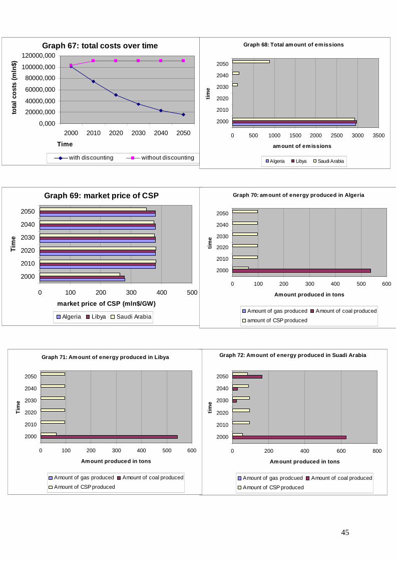
45


0 200 400 600 800

2000

2010

2020

2030

2040

2050

tim

e





0 100 200 300 400 500 600

2000

2010

2020

2030

2040

2050

Tim

e





0 100 200 300 400 500

2000

2010

2020

2030

2040

2050

Tim

e




0 100 200 300 400 500 600

2000

2010

2020

2030

2040

2050ti

me





0 500 1000 1500 2000 2500 3000 3500

2000

2010

2020

2030

2040

2050

tim

e

amount of emissions



0,000

20000,000

40000,000

60000,000

80000,000

100000,000

120000,000

2000 2010 2020 2030 2040 2050

Time

tota

l co

sts

(mln

$)


46

6. Conclusion In chapter 5 there are four different subjects with 3 scenarios each. All these scenario have different results. Now a general conclusion will be made using these twelve scenarios.

A price on emissions is a very effective instrument to reduce the amount of emissions (scenario 1B). When the total amount of emissions is restricted by a quantity restriction the amount of emissions will fall but not as fast as with a price on emissions (scenario 1C). Apparently the relative price of fossil fuels will be higher than the price of CSP when there are prices on emissions.

In this thesis the assumption is made that the three countries have the availability over the three energy sources compared. When there would be extra European demand for electricity this would be covered by producing electricity with coal (scenario 2B, scenario 2C). This is the most logical choice because coal is the cheapest energy source in this model. The only restriction thus is that there will be extra demand, this extra electricity demand will be covered by producing coal. With the political scenarios coals will also be used more to produce electricity. To meet the political minima (scenario 3B, scenario 3C) it is cheaper to produce coal then replacing this with CSP. There was no policy in reducing the amount of coal for political reasons. Therefore coal did not have a negative or a positive influence on the dependency factor. One could imagine that this would be the case and the coal would probably be produced less. The last subject are the prices for coal and gas. When the forecasted prices are used in the model (scenario 4B), the amounts of fossil fuels used to produce electricity will be drastically lower. The outcome of the scenario with extreme prices (scenario 4C) does not differ very much from the outcome with forecasted prices. This can be explained by the stable price of coal. Due to this stable price the extreme price stays low as compared to gas. Gas will not be used for producing electricity. The price of gas is much higher than the price of coal. In 2000 gas is already much more expensive. After 2000 the price of gas increases that much (scenario 4B) that this will not be used for producing electricity in the future. Coal has a much higher probability of being used for the production of electricity. The price of coal is already low in 2000 but it also stays very stable over time. There are enormous reserves of coal in the world, therefore the price of coal will be stable over time. This thus is the energy source where CSP has to compete with in the future. The scenario with the forecasted prices (scenario 4B) does give a positive signal that CSP will become a lot more attractive to produce in the future. This model does not take everything into account, so the effect will not be as positive as in this model. But the prices of fossil fuels are rising and therefore CSP will become more attractive. With the Kyoto protocol a quantity restriction on the amount of emissions is implemented in many countries. A quantity restriction (scenario 1B) is less effective than a price on emissions (scenario 1C). But in the end the result will be that the amount of emissions will be reduced. In the beginning the effect of a quantity restriction is very small but over time it will become more effective. I think that a price on emissions is hard to realize because this is so effective. Kyoto will reach their goal of reducing the amount of emissions with Concentrated Solar Panels. When the prices of fossil fuels will rise and the price of emissions will go down through innovation, ultimately CSP will become more attractive to produce electricity. The best place to construct CSP plants is Algeria. The overall distance to the European market is less than the overall distance to Libya. Further the amount of kilometres over water are also a lot less, which also makes Algeria more attractive. Algeria is not as politically

47

stable as Saudi Arabia but it is more stable then Libya. The costs for covering the distance are too high for Saudi Arabia. This becomes clear in all scenarios but especially in the scenario with higher prices for coal and gas (scenario 4b, scenario 4C). In these scenarios Saudi Arabia would use coal much faster to produce electricity then the other countries. This results in a lower demand for CSP from Saudi Arabia. The future thus is to produce CSP in the desert of Algeria.

48

References Internet sites References of internet sites are in alphabetic order: [afstandmeten, 2010] www.afstandemeten.nl Viewed on: 09-07-2010 [Bouwmans et al, 2006] http://www.tbm.tudelft.nl/live/binaries/ce78edc1-51a5-4d80-8d09-58e6ee8698db/doc/ConcentratedSolarPower-TUDelft.pdf Viewed on 07-07-2010 [Carbonemissions, 2009] http://www.carbonemissions.com/ Viewed on: 07-07-2010 [CPI, 2009] http://www.transparency.org/policy_research/surveys_indices/cpi/2009/cpi_2009_table Viewed on: 22-04-2010 [Douglas et al, 2008] http://www.fitcoalition.com/storage/documents/reesa-documents/FIT_Policy_Memo_to_CEC.pdf Viewed on: 07-07-2010 [Egerer et al, 2009] http://www.cni.tu-berlin.de/fileadmin/documents/infraday/2009/presentation/11e_egerer_v01_1pdf.pdf Viewed on: 07-07-2010 [EIA demand, 2008] http://tonto.eia.doe.gov/cfapps/ipdbproject/iedindex3.cfm?tid=2&pid=2&aid=2&cid=&syid=2000&eyid=2000&unit=BKWH Viewed on: 07-07-2010 [EIA emissions, 2000] http://www.eia.doe.gov/cneaf/electricity/page/co2_report/co2emiss.pdf Viewed on: 07-07-2010 [EIA market price electricity, 2010] http://www.eia.doe.gov/emeu/steo/pub/gifs/Fig23.gif Viewed on: 07-07-2010 [EIA price coal, 2008] http://www.eia.doe.gov/oiaf/aeo/pdf/trend_5.pdf Viewed on: 07-07-2010 [EIA price gas, 2008] http://www.eia.doe.gov/oiaf/aeo/pdf/trend_4.pdf Viewed on 07-07-2010 [Energyjustice gas, 2009] http://www.energyjustice.net/naturalgas/factsheet-ng.pdf (page 2, left side) Viewed on: 07-07-2010 [Energyjustice coal, 2007] http://www.energyjustice.net/coal/igcc/factsheet-long.pdf Viewed on: 07-07-2010 [Engineerlive, 2005]

49

http://www.engineerlive.com/Energy-Solutions/Transmition_Distribution/Underwater_HVDC_power_cable_sets_standard_for_transmission_projects/21325/ Viewed on: 07-07-2010 [Environmental leader, 2009] http://www.environmentalleader.com/2009/02/06/carbon-emissions-prices-drop-as-downturn-bites/ Viewed on: 07-07-2010 [EPA converter, 2009] http://www.epa.gov/cmop/resources/converter.html Viewed on: 07-07-2010 [Eurostat, 2007] http://www.energy.eu/publications/KSGB07001ENC_002.pdf Viewed on: 07-07-2010 [EVD Algeria, 2010] http://www.evd.nl/home/landen/landenpagina/land.asp?bstnum=63207&land=alg&location=/home/landen/landenpagina/land.asp?land=alg&highlight= Viewed on: 22-04-2010 [EVD Libya, 2010] http://www.evd.nl/home/landen/landenpagina/land.asp?bstnum=108382&land=lie&location=/home/landen/landenpagina/land.asp?land=lie&highlight= Viewed on: 22-04-2010 [Frontline, 2001] http://www.pbs.org/wgbh/pages/frontline/shows/saudi/interviews/ahmed.html Viewed on: 22-04-2010 [GAMS, 2010] http://www.gams.com/default.htm Viewed on: 10-05-2010 [Gately&Huntington, 2010] http://econ.as.nyu.edu/docs/IO/9187/RR01-01.PDF Viewed on: 07-07-2010 [GPI Algeria, 2009] http://www.visionofhumanity.org/gpi/results/algeria/2009/ Viewed on: 22-04-2010 [GPI Libya, 2009] http://www.visionofhumanity.org/gpi/results/libya/2009/ Viewed on: 22-04-2010 [GPI Saudi Arabia, 2009] http://www.visionofhumanity.org/gpi/results/saudi-arabia/2009/ Viewed on: 22-04-2010 [Kaufmann et al, 2006] http://siteresources.worldbank.org/INTWBIGOVANTCOR/Resources/1740479-1150402582357/2661829-1158008871017/gov_matters_5_tables.pdf Viewed on: 22-04-2010 [RNW, 2009] http://www.rnw.nl/data/files/images/Desertec%20div.%20productiemethoden%20en%20lokaties.jpg Viewed on: 13-07-2010 [Rudervall et al, 2005] http://www2.internetcad.com/pub/energy/technology_abb.pdf Viewed on: 07-07-2010

50

[Sindark, 2008] http://www.sindark.com/2008/01/07/hvdc-transmission-for-renewable-energy/ Viewed on: 07-07-2010 Books: [Varian, 2006] Varian, H., 2006. Intermediate Micro economics. Norton & Company. New York

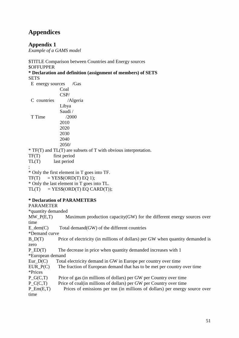
51

Appendices Appendix 1 Example of a GAMS model $TITLE Comparison between Countries and Energy sources $OFFUPPER * Declaration and definition (assignment of members) of SETS SETS E energy sources /Gas Coal CSP/ C countries /Algeria Libya Saudi / T Time /2000 2010 2020 2030 2040 2050/ * TF(T) and TL(T) are subsets of T with obvious interpretation. TF(T) first period TL(T) last period ; * Only the first element in T goes into TF. TF(T) = YES$(ORD(T) EQ 1); * Only the last element in T goes into TL. TL(T) = YES$(ORD(T) EQ CARD(T)); * Declaration of PARAMETERS PARAMETER *quantity demanded MW_P(E,T) Maximum production capacity(GW) for the different energy sources over time E_dem(C) Total demand(GW) of the different countries *Demand curve B_D(T) Price of electricity (in millions of dollars) per GW when quantity demanded is zero P_ED(T) The decrease in price when quantity demanded increases with 1 *European demand Eur_D(C) Total electricity demand in GW in Europe per country over time EUR_P(C) The fraction of European demand that has to be met per country over time *Prices P_G(C,T) Price of gas (in millions of dollars) per GW per Country over time P_C(C,T) Price of coal(in millions of dollars) per GW per Country over time P_Em(E,T) Prices of emissions per ton (in millions of dollars) per energy source over time

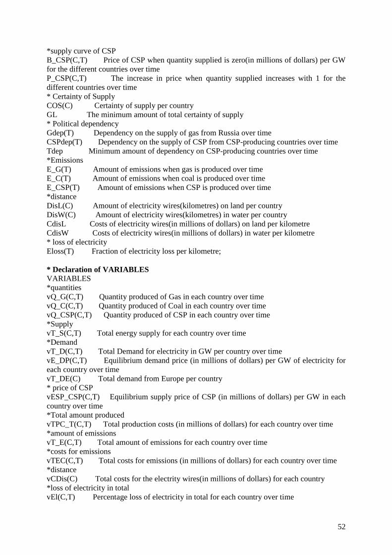
52

*supply curve of CSP B_CSP(C,T) Price of CSP when quantity supplied is zero(in millions of dollars) per GW for the different countries over time P_CSP(C,T) The increase in price when quantity supplied increases with 1 for the different countries over time * Certainty of Supply COS(C) Certainty of supply per country GL The minimum amount of total certainty of supply * Political dependency Gdep(T) Dependency on the supply of gas from Russia over time CSPdep(T) Dependency on the supply of CSP from CSP-producing countries over time Tdep Minimum amount of dependency on CSP-producing countries over time *Emissions E_G(T) Amount of emissions when gas is produced over time E_C(T) Amount of emissions when coal is produced over time E_CSP(T) Amount of emissions when CSP is produced over time *distance DisL(C) Amount of electricity wires(kilometres) on land per country DisW(C) Amount of electricity wires(kilometres) in water per country CdisL Costs of electricity wires(in millions of dollars) on land per kilometre CdisW Costs of electricity wires(in millions of dollars) in water per kilometre * loss of electricity Eloss(T) Fraction of electricity loss per kilometre; * Declaration of VARIABLES VARIABLES *quantities vQ_G(C,T) Quantity produced of Gas in each country over time vQ_C(C,T) Quantity produced of Coal in each country over time vQ_CSP(C,T) Quantity produced of CSP in each country over time *Supply vT_S(C,T) Total energy supply for each country over time *Demand vT_D(C,T) Total Demand for electricity in GW per country over time vE_DP(C,T) Equilibrium demand price (in millions of dollars) per GW of electricity for each country over time vT_DE(C) Total demand from Europe per country * price of CSP vESP_CSP(C,T) Equilibrium supply price of CSP (in millions of dollars) per GW in each country over time *Total amount produced vTPC_T(C,T) Total production costs (in millions of dollars) for each country over time *amount of emissions vT_E(C,T) Total amount of emissions for each country over time *costs for emissions vTEC(C,T) Total costs for emissions (in millions of dollars) for each country over time *distance vCDis(C) Total costs for the electrity wires(in millions of dollars) for each country *loss of electricity in total vEl(C,T) Percentage loss of electricity in total for each country over time

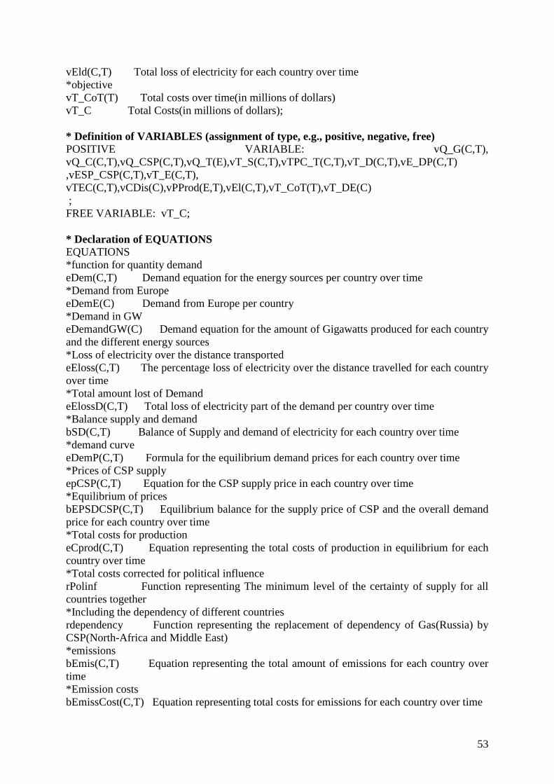
53

vEld(C,T) Total loss of electricity for each country over time *objective vT_CoT(T) Total costs over time(in millions of dollars) vT_C Total Costs(in millions of dollars); * Definition of VARIABLES (assignment of type, e.g., positive, negative, free) POSITIVE VARIABLE: vQ_G(C,T), vQ_C(C,T),vQ_CSP(C,T),vQ_T(E),vT_S(C,T),vTPC_T(C,T),vT_D(C,T),vE_DP(C,T) ,vESP_CSP(C,T),vT_E(C,T), vTEC(C,T),vCDis(C),vPProd(E,T),vEl(C,T),vT_CoT(T),vT_DE(C) ; FREE VARIABLE: vT_C; * Declaration of EQUATIONS EQUATIONS *function for quantity demand eDem(C,T) Demand equation for the energy sources per country over time *Demand from Europe eDemE(C) Demand from Europe per country *Demand in GW eDemandGW(C) Demand equation for the amount of Gigawatts produced for each country and the different energy sources *Loss of electricity over the distance transported eEloss(C,T) The percentage loss of electricity over the distance travelled for each country over time *Total amount lost of Demand eElossD(C,T) Total loss of electricity part of the demand per country over time *Balance supply and demand bSD(C,T) Balance of Supply and demand of electricity for each country over time *demand curve eDemP(C,T) Formula for the equilibrium demand prices for each country over time *Prices of CSP supply epCSP(C,T) Equation for the CSP supply price in each country over time *Equilibrium of prices bEPSDCSP(C,T) Equilibrium balance for the supply price of CSP and the overall demand price for each country over time *Total costs for production eCprod(C,T) Equation representing the total costs of production in equilibrium for each country over time *Total costs corrected for political influence rPolinf Function representing The minimum level of the certainty of supply for all countries together *Including the dependency of different countries rdependency Function representing the replacement of dependency of Gas(Russia) by CSP(North-Africa and Middle East) *emissions bEmis(C,T) Equation representing the total amount of emissions for each country over time *Emission costs bEmissCost(C,T) Equation representing total costs for emissions for each country over time

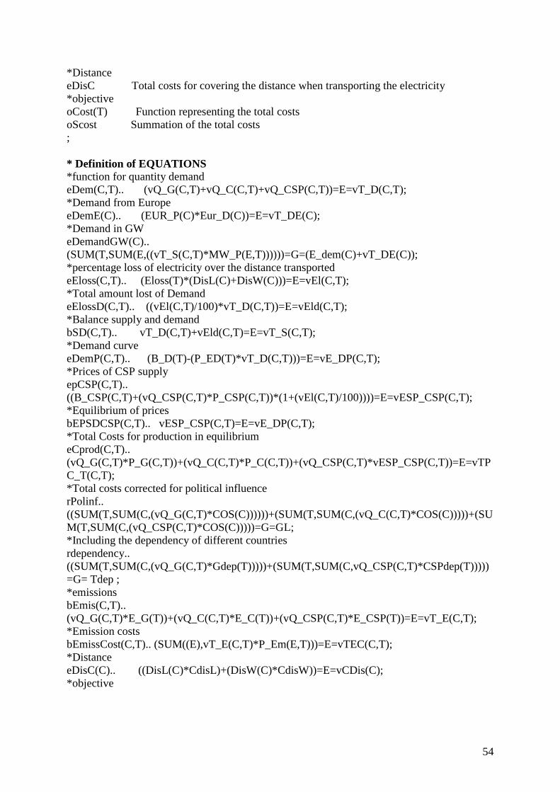
54

*Distance eDisC Total costs for covering the distance when transporting the electricity *objective oCost(T) Function representing the total costs oScost Summation of the total costs ; * Definition of EQUATIONS *function for quantity demand eDem(C,T).. (vQ_G(C,T)+vQ_C(C,T)+vQ_CSP(C,T))=E=vT_D(C,T); *Demand from Europe eDemE(C).. (EUR_P(C)*Eur_D(C))=E=vT_DE(C); *Demand in GW eDemandGW(C).. (SUM(T,SUM(E,((vT_S(C,T)*MW_P(E,T))))))=G=(E_dem(C)+vT_DE(C)); *percentage loss of electricity over the distance transported eEloss(C,T).. (Eloss(T)*(DisL(C)+DisW(C)))=E=vEl(C,T); *Total amount lost of Demand eElossD(C,T).. ((vEl(C,T)/100)*vT_D(C,T))=E=vEld(C,T); *Balance supply and demand bSD(C,T).. vT_D(C,T)+vEld(C,T)=E=vT_S(C,T); *Demand curve eDemP(C,T).. (B_D(T)-(P_ED(T)*vT_D(C,T)))=E=vE_DP(C,T); *Prices of CSP supply epCSP(C,T).. ((B_CSP(C,T)+(vQ_CSP(C,T)*P_CSP(C,T))*(1+(vEl(C,T)/100))))=E=vESP_CSP(C,T); *Equilibrium of prices bEPSDCSP(C,T).. vESP_CSP(C,T)=E=vE_DP(C,T); *Total Costs for production in equilibrium eCprod(C,T).. (vQ_G(C,T)*P_G(C,T))+(vQ_C(C,T)*P_C(C,T))+(vQ_CSP(C,T)*vESP_CSP(C,T))=E=vTPC_T(C,T); *Total costs corrected for political influence rPolinf.. ((SUM(T,SUM(C,(vQ_G(C,T)*COS(C))))))+(SUM(T,SUM(C,(vQ_C(C,T)*COS(C)))))+(SUM(T,SUM(C,(vQ_CSP(C,T)*COS(C)))))=G=GL; *Including the dependency of different countries rdependency.. ((SUM(T,SUM(C,(vQ_G(C,T)*Gdep(T)))))+(SUM(T,SUM(C,vQ_CSP(C,T)*CSPdep(T))))) =G= Tdep ; *emissions bEmis(C,T).. (vQ_G(C,T)*E_G(T))+(vQ_C(C,T)*E_C(T))+(vQ_CSP(C,T)*E_CSP(T))=E=vT_E(C,T); *Emission costs bEmissCost(C,T).. (SUM((E),vT_E(C,T)*P_Em(E,T)))=E=vTEC(C,T); *Distance eDisC(C).. ((DisL(C)*CdisL)+(DisW(C)*CdisW))=E=vCDis(C); *objective

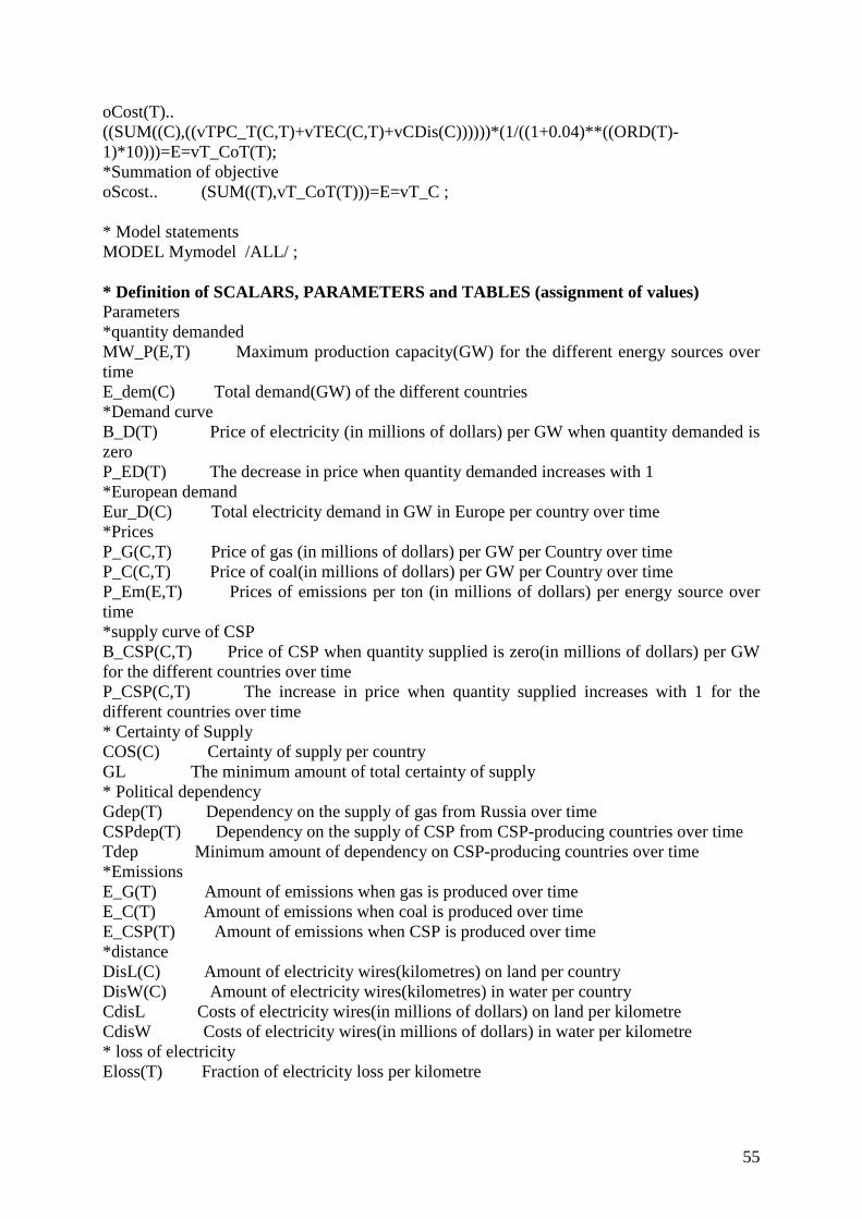
55

oCost(T).. ((SUM((C),((vTPC_T(C,T)+vTEC(C,T)+vCDis(C))))))*(1/((1+0.04)**((ORD(T)-1)*10)))=E=vT_CoT(T); *Summation of objective oScost.. (SUM((T),vT_CoT(T)))=E=vT_C ; * Model statements MODEL Mymodel /ALL/ ; * Definition of SCALARS, PARAMETERS and TABLES (assignment of values) Parameters *quantity demanded MW_P(E,T) Maximum production capacity(GW) for the different energy sources over time E_dem(C) Total demand(GW) of the different countries *Demand curve B_D(T) Price of electricity (in millions of dollars) per GW when quantity demanded is zero P_ED(T) The decrease in price when quantity demanded increases with 1 *European demand Eur_D(C) Total electricity demand in GW in Europe per country over time *Prices P_G(C,T) Price of gas (in millions of dollars) per GW per Country over time P_C(C,T) Price of coal(in millions of dollars) per GW per Country over time P_Em(E,T) Prices of emissions per ton (in millions of dollars) per energy source over time *supply curve of CSP B_CSP(C,T) Price of CSP when quantity supplied is zero(in millions of dollars) per GW for the different countries over time P_CSP(C,T) The increase in price when quantity supplied increases with 1 for the different countries over time * Certainty of Supply COS(C) Certainty of supply per country GL The minimum amount of total certainty of supply * Political dependency Gdep(T) Dependency on the supply of gas from Russia over time CSPdep(T) Dependency on the supply of CSP from CSP-producing countries over time Tdep Minimum amount of dependency on CSP-producing countries over time *Emissions E_G(T) Amount of emissions when gas is produced over time E_C(T) Amount of emissions when coal is produced over time E_CSP(T) Amount of emissions when CSP is produced over time *distance DisL(C) Amount of electricity wires(kilometres) on land per country DisW(C) Amount of electricity wires(kilometres) in water per country CdisL Costs of electricity wires(in millions of dollars) on land per kilometre CdisW Costs of electricity wires(in millions of dollars) in water per kilometre * loss of electricity Eloss(T) Fraction of electricity loss per kilometre

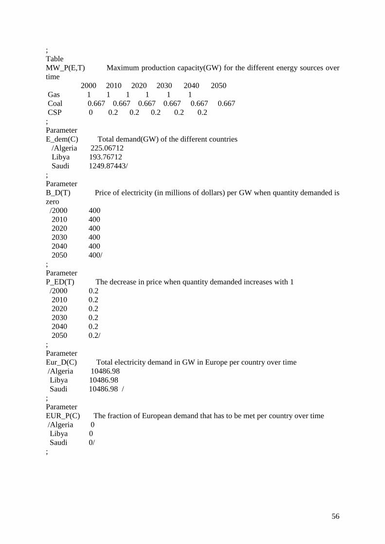
56

; Table MW_P(E,T) Maximum production capacity(GW) for the different energy sources over time 2000 2010 2020 2030 2040 2050 Gas 1 1 1 1 1 1 Coal 0.667 0.667 0.667 0.667 0.667 0.667 CSP 0 0.2 0.2 0.2 0.2 0.2 ; Parameter E_dem(C) Total demand(GW) of the different countries /Algeria 225.06712 Libya 193.76712 Saudi 1249.87443/ ; Parameter B_D(T) Price of electricity (in millions of dollars) per GW when quantity demanded is zero /2000 400 2010 400 2020 400 2030 400 2040 400 2050 400/ ; Parameter P_ED(T) The decrease in price when quantity demanded increases with 1 /2000 0.2 2010 0.2 2020 0.2 2030 0.2 2040 0.2 2050 0.2/ ; Parameter Eur_D(C) Total electricity demand in GW in Europe per country over time /Algeria 10486.98 Libya 10486.98 Saudi 10486.98 / ; Parameter EUR_P(C) The fraction of European demand that has to be met per country over time /Algeria 0 Libya 0 Saudi 0/ ;

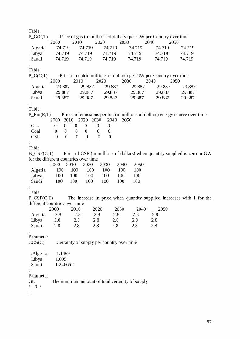
57

Table P_G(C,T) Price of gas (in millions of dollars) per GW per Country over time 2000 2010 2020 2030 2040 2050 Algeria 74.719 74.719 74.719 74.719 74.719 74.719 Libya 74.719 74.719 74.719 74.719 74.719 74.719 Saudi 74.719 74.719 74.719 74.719 74.719 74.719 ; Table P_C(C,T) Price of coal(in millions of dollars) per GW per Country over time 2000 2010 2020 2030 2040 2050 Algeria 29.887 29.887 29.887 29.887 29.887 29.887 Libya 29.887 29.887 29.887 29.887 29.887 29.887 Saudi 29.887 29.887 29.887 29.887 29.887 29.887 ; Table P_Em(E,T) Prices of emissions per ton (in millions of dollars) energy source over time 2000 2010 2020 2030 2040 2050 Gas 0 0 0 0 0 0 Coal 0 0 0 0 0 0 CSP 0 0 0 0 0 0 ; Table B_CSP(C,T) Price of CSP (in millions of dollars) when quantity supplied is zero in GW for the different countries over time 2000 2010 2020 2030 2040 2050 Algeria 100 100 100 100 100 100 Libya 100 100 100 100 100 100 Saudi 100 100 100 100 100 100 ; Table P_CSP(C,T) The increase in price when quantity supplied increases with 1 for the different countries over time 2000 2010 2020 2030 2040 2050 Algeria 2.8 2.8 2.8 2.8 2.8 2.8 Libya 2.8 2.8 2.8 2.8 2.8 2.8 Saudi 2.8 2.8 2.8 2.8 2.8 2.8 ; Parameter COS(C) Certainty of supply per country over time /Algeria 1.1469 Libya 1.095 Saudi 1.24665 / ; Parameter GL The minimum amount of total certainty of supply / 0 / ;

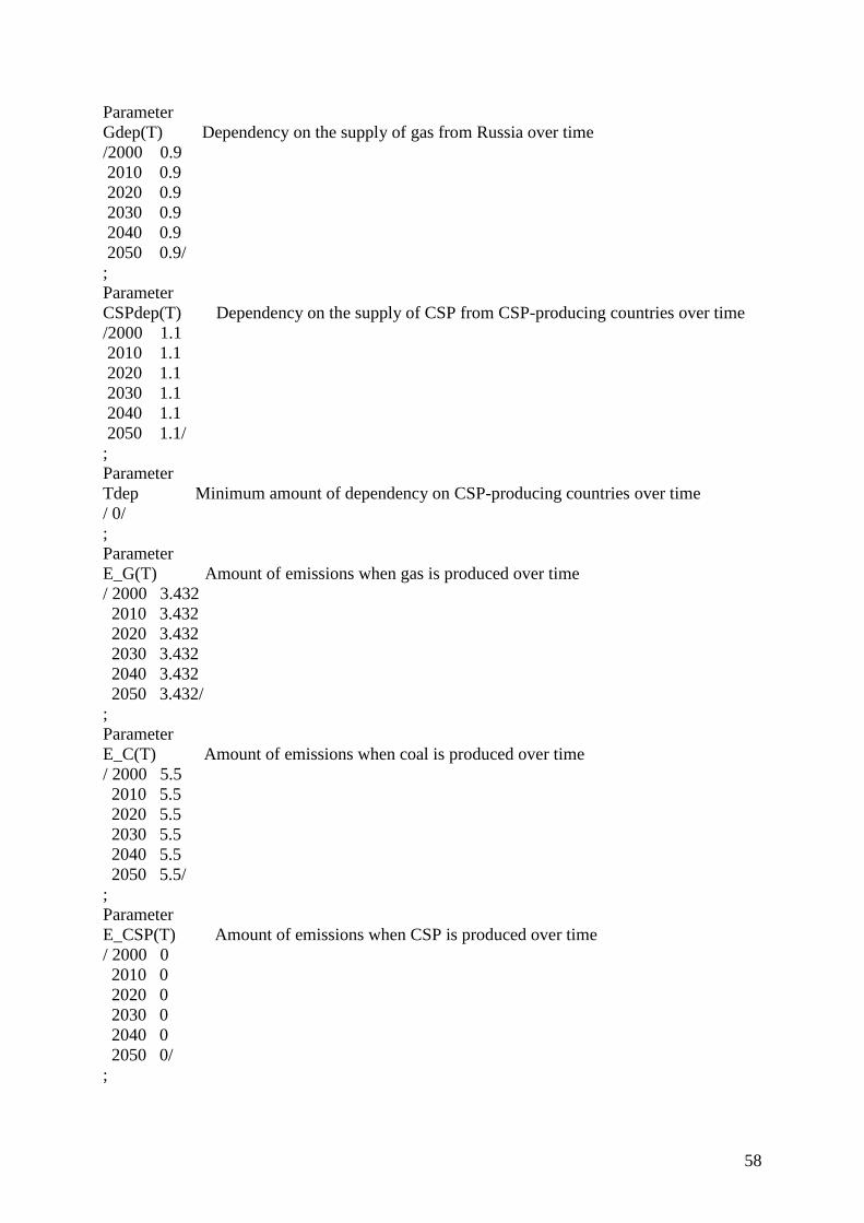
58

Parameter Gdep(T) Dependency on the supply of gas from Russia over time /2000 0.9 2010 0.9 2020 0.9 2030 0.9 2040 0.9 2050 0.9/ ; Parameter CSPdep(T) Dependency on the supply of CSP from CSP-producing countries over time /2000 1.1 2010 1.1 2020 1.1 2030 1.1 2040 1.1 2050 1.1/ ; Parameter Tdep Minimum amount of dependency on CSP-producing countries over time / 0/ ; Parameter E_G(T) Amount of emissions when gas is produced over time / 2000 3.432 2010 3.432 2020 3.432 2030 3.432 2040 3.432 2050 3.432/ ; Parameter E_C(T) Amount of emissions when coal is produced over time / 2000 5.5 2010 5.5 2020 5.5 2030 5.5 2040 5.5 2050 5.5/ ; Parameter E_CSP(T) Amount of emissions when CSP is produced over time / 2000 0 2010 0 2020 0 2030 0 2040 0 2050 0/ ;

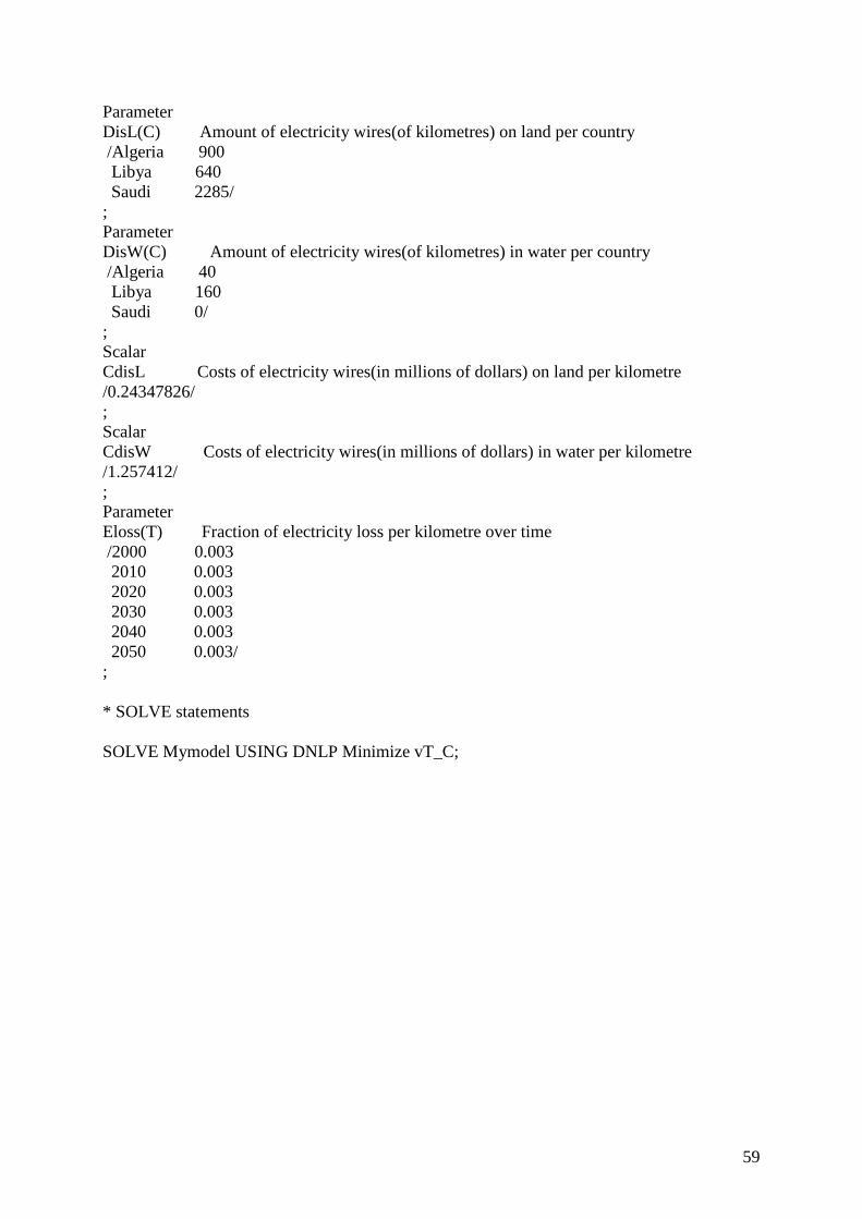
59

Parameter DisL(C) Amount of electricity wires(of kilometres) on land per country /Algeria 900 Libya 640 Saudi 2285/ ; Parameter DisW(C) Amount of electricity wires(of kilometres) in water per country /Algeria 40 Libya 160 Saudi 0/ ; Scalar CdisL Costs of electricity wires(in millions of dollars) on land per kilometre /0.24347826/ ; Scalar CdisW Costs of electricity wires(in millions of dollars) in water per kilometre /1.257412/ ; Parameter Eloss(T) Fraction of electricity loss per kilometre over time /2000 0.003 2010 0.003 2020 0.003 2030 0.003 2040 0.003 2050 0.003/ ; * SOLVE statements SOLVE Mymodel USING DNLP Minimize vT_C;

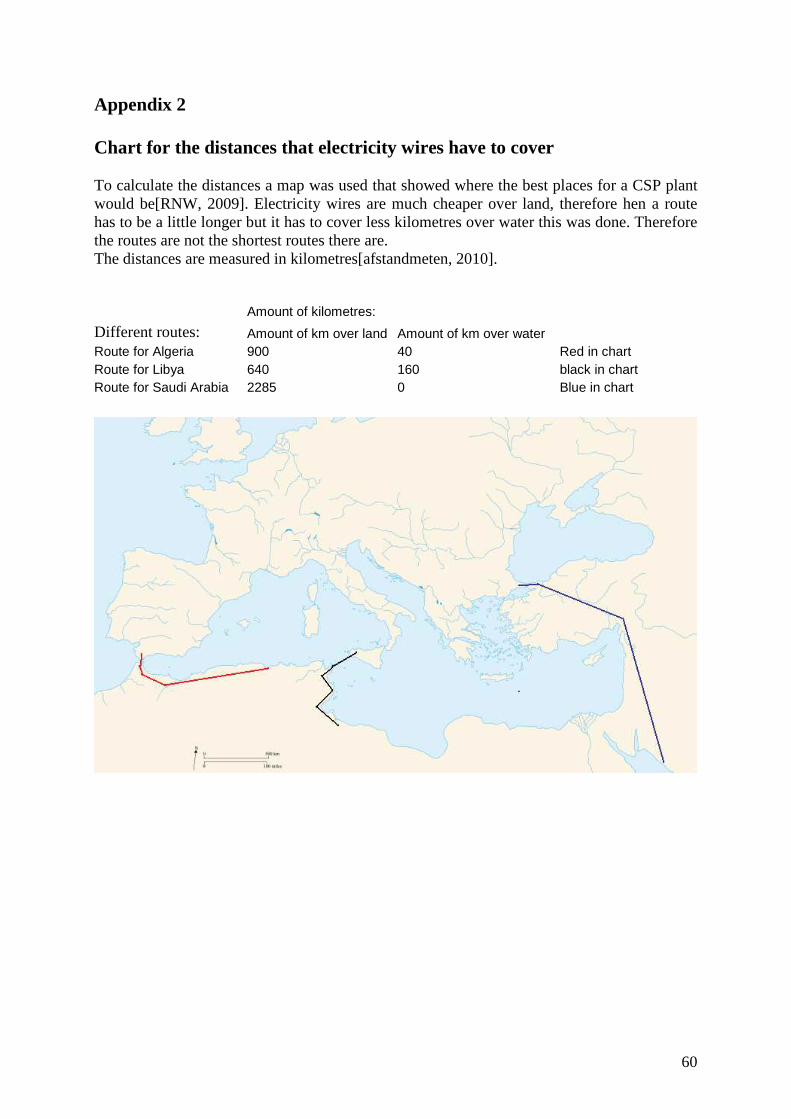
60

Appendix 2 Chart for the distances that electricity wires have to cover To calculate the distances a map was used that showed where the best places for a CSP plant would be[RNW, 2009]. Electricity wires are much cheaper over land, therefore hen a route has to be a little longer but it has to cover less kilometres over water this was done. Therefore the routes are not the shortest routes there are. The distances are measured in kilometres[afstandmeten, 2010].

Amount of kilometres: Different routes: Amount of km over land Amount of km over water Route for Algeria 900 40 Red in chart Route for Libya 640 160 black in chart Route for Saudi Arabia 2285 0 Blue in chart

Documents

Solar energy; the solution for the rising electricity demand?