Embed Size (px)
Citation preview
Please cite this paper as:
No. 190
What Happens to Wage Elasticities
When We Strip Playometrics?
Revisiting Married Women Labour
Supply Model
by
Duo Qin, Sophie van Huellen and Qing-Chao
Wang
(December, 2014)
Department of Economics
School of Oriental and African Studies
London
WC1H 0XG
Phone: + 44 (0)20 7898 4730 Fax: 020 7898 4759
E-mail: [email protected]
http://www.soas.ac.uk/economics/
Dep
art
men
t o
f E
con
om
ics
Working Paper Series
ISSN 1753 - 5816
Qin, D., S. van Huellen and Q-C. Wang. (2014), “What Happens to Wage Elasticities When
We Strip Playometrics? Revisiting Married Women Labour Supply Model”, SOAS
Department of Economics Working Paper Series, No. 190, The School of Oriental and
African Studies.
The SOAS Department of Economics Working Paper Series is published electronically by The
School of Oriental and African Studies-University of London.
©Copyright is held by the author or authors of each working paper. SOAS DoEc Working Papers
cannot be republished, reprinted or reproduced in any format without the permission of the paper’s
author or authors.
This and other papers can be downloaded without charge from:
SOAS Department of Economics Working Paper Series at
http://www.soas.ac.uk/economics/research/workingpapers/
Research Papers in Economics (RePEc) electronic library at
http://econpapers.repec.org/paper/
Design and layout: O.G. Dávila
SOAS Department of Economics Working Paper Series No 190 - 2014
1
What Happens to Wage Elasticities When We Strip Playometrics?
Revisiting Married Women Labour Supply Model
Duo Qin, Sophie van Huellen, Qing-Chao Wang*
Abstract
This paper sheds new light on the well-known phenomenon of dwindling wage elasticities for
married women in the US over the recent decades. Results of a novel model experiment
approach via sample data ordering unveil considerable heterogeneity across different wage
groups. Yet surprisingly constant wage elasticity estimates are revealed within certain wage
groups over time as well as across two widely used US data sources, the Current Population
Survey (CPS) and the Panel Study of Income Dynamics (PSID). These findings refute the
assumed presence of a single-valued aggregate wage elasticity for working wives. Although
women’s responsiveness to wages remains largely unchanged over time, we find that the
composition of working women into different wage groups has changed considerably, resulting
in decreasing wage elasticity estimates at the aggregate level. All these findings were
methodologically impossible to acquire had we not dismantled and discarded the stereotyped
endogeneity-backed instrumental variable route, which hitherto blocked the way towards
sample data ordering.
Keywords: instrumental variable, labour supply wage elasticity, parameter stability, selection
bias.
JEL classification: J22, C18, C52, C55
* Duo Qin, Sophie van Huellen, and Qing-Chao Wang are from SOAS, University of London, UK; Duo Qin is
the contacting author, email: [email protected].
SOAS Department of Economics Working Paper Series No 190 - 2014
2
1. Introduction
The relative responsiveness of female workers to changes in wages and income is at the
core of labour economics. Historically women’s wage elasticity is found to be considerably
higher relative to their male counterparts (Killingsworth 1983, Heckman 1993). The theoretical
premise for this is that the income effect for women is small while the substitution effect
dominates. This is usually explained by the traditional division of labour within families where
wives are assumed to substitute between household tasks, market work, and leisure while men
only substitute between the latter two. Since household tasks and market work are close
substitutes, the wage substitution effect is arguably large for women which results in a positive
uncompensated wage effect (income and substitution effect) and relative elastic female labour
supply with respect to wage rate, e.g. see Mincer (1962). More recent empirical studies
challenge this gap between male and female wage elasticities and observe shrinking elasticities
for married women in the US. For instance, Blau and Kahn (2007) find a steady and dramatic
reduction in women’s wage elasticity by about 50 to 56 per cent during the 1980-2000 period,
with respect to both labour force participation and hours of work. Likewise, Heim (2007)
observes a 60 to 95 per cent reduction in intensive and extensive margins from 1979 to 2003.
The dwindling elasticity has become almost a stylised fact, e.g. see McClelland and Mok
(2012). Theoretically, these developments are linked to disbanding traditional gender roles
(Goldin 1990) and increasing wage opportunities for women (Juhn and Murphy 1997).
Empirical studies on the wage elasticity gap between males and females are
predominantly executed at a micro level. However, microeconomic estimations are everything
but uncontroversial and elasticity estimates vary substantially across studies (Killingsworth
and Heckman 1986, Blundell and MaCurdy 1999). Furthermore, microeconomic estimates of
labour supply elasticities based on hours of work tend to be smaller than elasticities implied by

SOAS Department of Economics Working Paper Series No 190 - 2014
3
macroeconomic models of fluctuations in aggregated hours of work over the business cycle
(Keane and Rogerson 2012). Although studies suggest taking the microeconomic estimate for
calibrating aggregated macroeconomic models (Cetty, et al. 2011), such process has been
heavily criticised (Peterman 2014, Fiorito and Zanella 2012) and no consensus has been found
yet. This unresolved anomaly between macro and micro results as well as the variety of
estimates presented by micro models alone put into questions the general reliability or
credibility of wage elasticity estimates.
The purpose of this study is twofold: Firstly, the conventional methods for modelling
wage elasticity of labour supply are challenged. Secondly, against the background of this
critique, a potential way forward is proposed. In particular, the paper targets the instrumental
variable (IV) approach to endogeneity, which is further compounded by Heckman’s selection
bias correction. The IV treatment arises originally from a concern over circular causality
between the wage-rate and hours worked. Such an approach is questionable in the present case
of married women’s labour supply on both economic and econometric grounds. From an
economic perspective, it is seriously doubtful whether the majority of working women have
the bargaining power to influence their wage rate and it might indeed be reasonable to assume
that the great majority are wage takers, which renders the concern for endogeneity
substantively superfluous. From an econometric perspective, the IV approach is based on
rejecting the wage rate as a valid conditional variable for hours of work and replace it by non-
optimal and hence non-unique predictors of this variable. These predictors are generated from
instruments which are chosen on the basis of statistical correlation alone rather than causal
reasoning, e.g. see Qin (2014a). Such treatment, as will be shown in the following, results in
frequent violation of over identification restrictions and obstruction of systematic data learning
to locate statistically robust wage elasticity estimates.
SOAS Department of Economics Working Paper Series No 190 - 2014
4
In the same vain it is argued that the Heckman selection bias correction procedure is
redundant since it targets at the possible omitted variable bias (OVB) of the individual
parameter estimates in the instrumented wage equation rather than the hours of work equation.
The procedure amounts to adding an additional instrument to the already over-identified and
poorly fitted-wage equation which is relatively insensitive to the addition of the correction.
This correction is motivated by the fact that the offering wage is unobserved for non-working
individuals. While selection bias is a potential concern, depending on the target group, the
conventional approach is shown to not enter the parameter of interest significantly for the
present case.
We maintain that the IV approach and its selection-bias correction variations are not
simply a technical issue of estimator choice for applied modellers, but pose a methodological
block to empirical data discovery. By breaking with the textbook paradigm, we are able to
suggest a constructive way towards more credible wage elasticity estimates by sample data
ordering. This approach is not only close to the economic interpretation of wage elasticities,
but also yields additional insights into the nature of wage elasticities within various samples of
married working women. In particular, it is shown that wage elasticity parameters vary
substantially across different wage groups and even turn negative for high wage earners; an
effect which is hidden under the textbook approach. By sample ordering we are, however, able
to locate a wage range within which wage elasticity parameters are constant, positive and
highly significant. We show that this wage range and parameter estimates are surprisingly
invariant across different waves, while the share of women falling within this wage range
varies.
These findings shed new light on the two almost established economic phenomena of
shrinking elasticities for married women in the US and the gap between micro and macro
elasticities. We argue that the finding of shrinking elasticities is actually a result not of changes
SOAS Department of Economics Working Paper Series No 190 - 2014
5
in disaggregate elasticities per se but a shifting composition of working women in different
wage segments over the last decades. Further, the discovery of significant heterogeneity among
working women puts into question the assumption of single valued micro elasticities and calls
for a theoretical reorientation for those aiming to align micro with macro estimates.
The microeconomic female labour supply model is commonly estimated taking married
women at their prime working age with working husbands as the target group. We will follow
this approach taking two widely used US based cross-section data sources into consideration –
the Current Population Survey (CPS) and the Panel Study of Income Dynamics (PSID). The
parallel use of the CPS and PSID sources provide us with a powerful means of cross-checking
the degrees of inferability between samples. For estimation the years 1980, 1990, 1999, 2003,
2007, and 2011 are chosen. These firstly coincide with the time periods investigated by two
core papers, Blau and Kahn (2007) and Heim (2007) which are based on CPS data, and hence
make a good comparative case1 and secondly go beyond the time frame previously analysed.
A detailed description of the datasets and processing of the data can be found in Appendix 1.
The remainder of the paper proceeds as follow. Section 2 dismantles the textbook
approach to wage elasticity estimation by revealing fundamental flaws in the endogeneity-
backed IV approach and selection bias correction treatment of the wage variable. Section 3
picks up the pieces and suggest alternatives towards a more credible wage elasticity estimate.
Section 4 concludes and provides an outlook for future research.
2. How Superfluous Are Endogeneity and Selection Bias Correction Treatments?
The most commonly used empirical model of labour supply for married women with
respect to cross-section data is:
(1) 𝐻𝑖 = 𝛼0 + 𝛼1𝑙𝑛(𝑤𝑖) + 𝛼2𝑙𝑛(𝐼𝑖) + ∑ 𝛽𝑖𝑗𝑋𝑖𝑗𝑗 + 휀𝑖
1 Blau and Kahn (2007) pool 1979-81, 1989-91 and 1999-2001 into three samples. We simply choose one mid
wave for each of the three. However, we choose 1999 for the third wave because the PSID source does not provide
2000 data.
SOAS Department of Economics Working Paper Series No 190 - 2014
6
where 𝐻𝑖 denotes wife’s total hours of work in household i, 𝑤𝑖 her wage rate, 𝐼𝑖 her husband
wage rate or income, and {𝑋𝑖𝑗} a set of explanatory variables of demographic characteristics,
such as wife’s age, education, work experience and the number of children in the household.
𝛼1 and 𝛼2 are the parameters of interest for the purpose of measuring the hours wage elasticity
and hours income elasticity respectively. Here, it suffices our methodological exposition to be
focused on the measurement issues around 𝛼1 alone.
It is almost standard practice2 to estimate model (1) via an IV treatment to 𝑤𝑖 out of two
major concerns – endogeneity and selection bias.3 Specifically, the static relationship between
𝐻𝑖 and 𝑤𝑖, in (1) associates easily to the classical case of a simultaneous equation model (SEM)
between quantity and price, which is widely taught in textbooks. Meanwhile, the observed 𝑤𝑖
is believed to suffer from ‘selection bias’ due to lack of information on what the offering wages
might be for those non-working housewives in cross-section data. The IV treatment demands
re-specifying (1) into a two-equation model:
(2) 𝐻𝑖 = 𝛼0 + 𝛼1𝑙𝑛(𝑤𝑖)̂
𝐼𝑉 + 𝛼2𝑙𝑛(𝐼𝑖) + ∑ 𝛽𝑖𝑗𝑋𝑖𝑗𝑗 + 휀𝑖
𝑙𝑛(𝑤𝑖) = 𝜆0 + ∑ 𝜆𝑖𝑘𝑍𝑖𝑘𝑘 + 𝑢𝑖 ⇒ 𝑙𝑛(𝑤𝑖)̂𝐼𝑉
which underlies the two stage least square (2SLS) estimation procedure of IV models. In
equation (2), {𝑍𝑖𝑗} is a set of IVs such that 𝑍 ⊋ {𝑙𝑛(𝐼), 𝑋}. When selection bias is of concern,
an inverse Mills ratio, 𝜌, is commonly included in Z. The ratio is derived from the residual
density function of the following binary response model of labour force participation:
(3) 𝑃𝑖 = 𝜃0 + 𝜃2𝑙𝑛(𝐼𝑖) + ∑ 𝜅𝑖𝑚𝑌𝑖𝑚𝑚 + 𝜖𝑖 𝑃𝑖 = {
1 𝑖𝑓 𝑤𝑖 > 00 𝑖𝑓 𝑤𝑖 = 0
𝜌 =𝜙(𝜖𝑖)
Φ(𝜖𝑖)
2 This can be seen from both the wide adoption of Mroz’s (1987) study in econometrics textbooks, e.g. Berndt
(1991), and the extensive use of IV and 2SLS methods in labour economics research, e.g. see Moffitt (1999). 3 Another issue of concern is omitted variable bias (OVB). This issue is left aside here mainly for two reasons.
First and obviously, it helps us to be more focused on the other two issues. Secondly, OVB should not be a serious
problem for the wage parameter estimation in our model because its log specification and value-continuous
property within the working population deems its correlations with potentially omitted variables, such as
geographic location, tax rate, quite low and unlikely invariant in large samples.
SOAS Department of Economics Working Paper Series No 190 - 2014
7
where {𝑙𝑛(𝐼), 𝑌} ⊋ 𝑍. Probit is normally used to estimate (3) according to the Heckman two-
step procedure (1979).
The underlying reasoning for hours of work being causal for wage-rates lies in the
assumption that the harder (more hours) one works, the higher the reward (wage rate).
However, there lacks economic ground to assume that married women in general should have
the wage bargaining power through their choice of working hour supply. Even if assuming a
certain bargaining power this probably arises from seniority and status at the workplace and
union representation rather than hours worked (Gersuny 1982). Hence, the endogeneity
specification in (2) is substantively superfluous.
However, model (2) is a pseudo SEM in that 𝑙𝑛(𝑤𝑖) is not simultaneously determined by
𝐻𝑖. In fact, the corresponding IV treatment amounts to rejecting 𝑙𝑛(𝑤𝑖) as a valid conditional
variable for 𝐻𝑖 and accepting, instead, 𝑙𝑛(𝑤𝑖)̂𝐼𝑉, a non-optimal predictor of 𝑙𝑛(𝑤𝑖), as the valid
conditional variable (see Qin (2014a) for a detailed exposition). The non-optimality of 𝑙𝑛(𝑤𝑖)̂𝐼𝑉
is easy to see in the context of large cross-section survey samples, because it is virtually
impossible to get 𝑙𝑛(𝑤𝑖)̂𝐼𝑉 close to 𝑙𝑛(𝑤𝑖) enough to yield a statistically identical �̂�1
𝐼𝑉, the IV
estimate from equation (2), to �̂�1𝑂𝐿𝑆 from equation (1). Consequently, confirmation of the
Durbin-Wu-Hausman endogeneity test, a test on �̂�1𝐼𝑉 ≠ �̂�1
𝑂𝐿𝑆, is usually achievable. Moreover,
the chance of obtaining statistically significant estimates of 𝛼1 becomes higher under the IV
treatment compared to OLS, thanks to the non-uniqueness of 𝑙𝑛(𝑤𝑖)̂𝐼𝑉 which results from the
very nature of non-optimality.
The above discussion tells us that it is empirically crucial to determine whether we can
reject 𝑙𝑛(𝑤𝑖) as a valid conditional variable in (1) in favour of a non-optimal predictor of it as
specified in the second equation in (2). Here, we examine this issue from three respects. (i) We
examine the validity of IVs by over-identification restriction tests; (ii) we examine the degree
SOAS Department of Economics Working Paper Series No 190 - 2014
8
of simultaneity between 𝑙𝑛(𝑤𝑖) and 𝐻𝑖 by running a genuine SEM; and (iii) we examine the
invariance property of �̂�1𝐼𝑉 across difference samples.
Textbooks tell us that valid IVs have to be correlated with the suspected ‘endogenous’
explanatory variables and uncorrelated with other explanatory variables, and that this condition
is not testable unless the model is over-identified, i.e. chosen IVs outnumber the suspected
‘endogenous’ explanatory variables. Fortunately, the just-identification case, i.e. 𝑘 = 1, does
not apply to (2) almost surely because it is virtually impossible to get reasonably good fits of
𝑙𝑛(𝑤𝑖) from multiple regression models using large cross-section data, a problem known as
the weak IV problem (see Bound, et al. (1995)). Hence, the validity of {𝑍𝑖𝑗} is largely testable.
What poses as a problem is the non-uniqueness in choosing the IVs. To circumvent this
problem, we start our experiment by trying to produce �̂�1𝐼𝑉 in line with some existing estimates
reported in the literature. The two cases that we choose are Blau and Kahn (2007) and Heim
(2007). Since both papers have reported results for three waves of the CPS data 1980, 1990,
2000, we aim to get our �̂�1𝐼𝑉 as close as possible to what is reported in those two papers, even
our models do not cover all the explanatory variables used by them.4 Specifically, two groups
of experiments are produced. The first group is carried out aiming for a set of IVs which would
get us close to the above two cases using the CPS data, and apply the same set of instruments
to the PSID data. The second group is carried out seeking a set of IVs for the same purpose
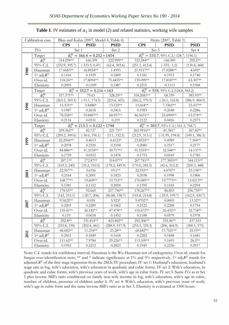
using the PSID data alone. Table 1 provides the key results of these experiments.
Several common features are discernible from Table 1. It is not difficult to find IV
estimates using the CPS samples which corroborate our targeted values even though our model
does not have the same variable coverage as the papers presenting the results we seek to
replicate (see the two CPS columns). However, the corroboration is not reproducible when we
4 As explained in footnote 1, we take 1999 wave here as a proxy for 2000, due to the fact that the PSID source
does not have 2000 survey.
SOAS Department of Economics Working Paper Series No 190 - 2014
9
apply the same IV set to the PSID data of the same waves (see columns 2 and 5), indicating
low degrees of statistical inferability. This goes against the expectation that CPS surveys should
be adequately representative with respect to the PSID surveys. Nevertheless, corroboration of
the targeted values is still achievable through alteration of the IV set (see columns 3 and 6).
These experiments clearly demonstrate the non-uniqueness of the IV route. As expected,
𝑙𝑛(𝑤𝑖)̂𝐼𝑉 obtained from the various sets of the first-stage of the IV procedure are substantially
different from 𝑙𝑛(𝑤𝑖), as easily seen from those small adjusted 𝑅2 statistics reported in Table
1, in spite of that equation being ‘over-identified’. Consequently, the Durbin-Wu-Hausman
endogeneity test statistics endorse the IV estimates for the majority of cases for being different
from the OLS estimates. However, the Sargan over-identification restriction test is rejected
dominantly, invalidating all of the four IV sets. The rejection comes unsurprisingly since 𝑍 ∩
{𝑙𝑛(𝐼), 𝑋} ≠ 0 for all our IV sets, though violation of the correlation condition is somewhat
eased by taking quadratic or cubit forms of the overlapping variables.
It is noticeable from Table 1 that those IV estimates with selection-bias corrections do
not show much statistically significant difference as compared with the general varied ranges
of IV estimates (compare the two CPS columns, or columns 2 and 5 in the PSID case). This
finding corroborates many previous findings including Blau and Kahn (2007) and Newey, et
al. (1990). It demonstrates how superfluous the conventional selection-bias correction is for
the present case. The superfluousness is actually implied in the IV-based model (2), where the
correction amounts to adding one more instrument, 𝜌, in the already over-identified IV set, Z.
Furthermore, this additional instrument, 𝜌, is derived from instruments, Y, which carry notably
overlapping information with Z. Conceptually, substantive concerns over selection bias is with
respect to the ‘missing’ offering wage rate, not with hours of work. Here, it is epistemologically
vital to see that Heckman’s method is not designed to resolve the possible misrepresentation
problem in making statistical inference, which is based merely on observable wage
SOAS Department of Economics Working Paper Series No 190 - 2014
10
information, beyond the working population. Rather, the method targets, on the assumption
that selection bias exists, narrowly at the possible OLS bias in modelling the wage variable and
treats the bias as a special type of omitted variable bias (OVB) (see Heckman (1976)). In our
present case, the Heckman method is focused on correcting the possible OVB in 𝜆𝑖𝑘 estimated
by the OLS in the IV equation of (2). Obviously, the correction is beside the point in view of
estimating our parameter interest, 𝛼1. Numerous empirical model results tell us that the
estimates of 𝛼1 are sensitive to the choice of 𝑙𝑛(𝑤𝑖)̂𝐼𝑉, as illustrated in Table 1. In contrast,
𝑙𝑛(𝑤𝑖)̂𝐼𝑉 is usually not sensitive, as measured either by the adjusted R2 or any information
criteria, to whether the estimated 𝜆𝑖𝑘 suffer from OVB due to missing 𝜌, especially when 𝜌 is
based on heavily overlapping Z and {𝑙𝑛(𝐼), 𝑌}.5
Here, what is probably more relevant than ‘selection bias’ is the truncation effect in 𝐻𝑖.6
In order to assess this effect via nonlinear estimation such as tobit, we need to impute the
‘missing’ offering wage rates. Considering the unsatisfactorily low fit of various regression
models or likelihood based methods previously used in the literature, we decide to use the hot
deck imputation method here to impute the missing offering wage rates. This method has been
widely used by statisticians for handling missing data, e.g. see Andridge and Little (2010), and
can be seen as a systematic extension to the method used by Blau and Kahn (2007). The details
of our imputation are described in Appendix 2.
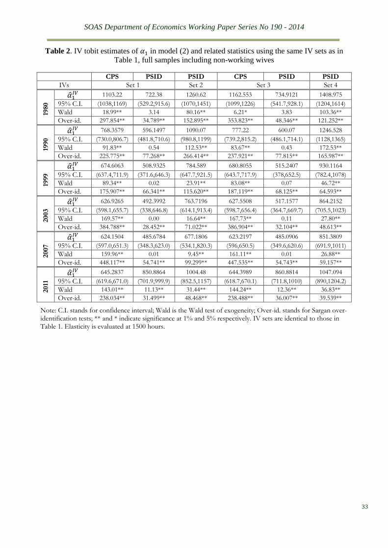
Once those ‘missing’ offering wage rates are imputed, we re-estimate (2) with the IV
tobit method using extended data samples including those wives having zero work hours. The
main results are summarised in Table 2. It is remarkable how substantially different the IV
5 This is multicollinear issue and formally demonstrated by Puhani (2000), whereas the similarity of the Heckman
correction to the simple OLS correction is shown by Olsen (1980). 6 It is debatable whether we should use model (1) to characterise the labour supply behaviour of both the working
group and non-working group. The truncation effect would not matter here if we assume that wage effect on hours
of work differ from that on the labour force participation. This assumption finds support from our subsequent
experiment reported in Section 3. Nevertheless, we have tried the tobit route following the practice of Blau and
Kahn (2007).
SOAS Department of Economics Working Paper Series No 190 - 2014
11
estimates are as compared to those reported in Table 1. The only feature which remains
unchanged is the wide acceptance of the ‘endogeneity’ test jointly with sweeping rejection of
the over-identification restrictions. Since the truncation effect on the OLS bias has been shown
to be approximately a rescale effect by the shares of the truncated observations in a truncated
sample, (see Greene (1981) and Cheung and Goldberger (1984)) we re-run the extended
samples simply by the tobit and the OLS, and then calculate the scaled OLS estimates. As seen
from Table 3, the scaled OLS estimates are indeed very similar to the tobit estimates. The extra
amount of variations in IV tobit estimates in Table 2 as compared to those in Table 1 cannot
be possibly accounted for as the truncation effect. The non-optimality of this IV route is too
apparent to deserve further comments.
Next, we extend model (1) into a genuine SEM:
(4) 𝐻𝑖 = 𝛼0 + 𝛼1𝑙𝑛(𝑤𝑖) + 𝛼2𝑙𝑛(𝐼𝑖) + ∑ 𝛽𝑖𝑗𝑋𝑖𝑗𝑗 + 휀𝑖
𝑙𝑛(𝑤𝑖) = 𝛾0 + 𝛾1𝐻𝑖 + ∑ 𝛿𝑖𝑗𝑍𝑖𝑗𝑙𝑗=1 + 𝜐𝑖
and estimate it by the FIML (full-information maximum likelihood) method. Notice, (4)
augments (2) by adding 𝐻𝑖 in its second equation. Hence, over-identification restriction tests
still apply here. Table 5 reports the main results of this experiment. Again, the over-
identification restriction test is rejected in all of the cases. Notice that more than half of the
cases fail to demonstrate the presence of significant simultaneity between 𝛼1 and 𝛾1 estimates.
Worse still, the majority of the wage parameter estimates are now negative, making them far
less credible than those IV estimates given in Table 1. In fact, the incredibility of these SEM
results have been exposed repeatedly before in macro-econometrics, e.g. see Qin (1993, 2013).
In particular, the insurmountable gap between reality and those over-identification restrictions
used to circumvent endogeneity created by simple model formulation has also been forcefully
criticised (e.g. Sims (1980)).
It is also easily noticeable from tables 1, 2 and 5 how different the IV and FIML estimates
can be between the CPS and PSID samples of the same waves. Since parameter invariance
SOAS Department of Economics Working Paper Series No 190 - 2014
12
plays such a fundamental role in statistical inference, our next experiment turns to the degrees
of within-sample invariance.7 This is carried out via recursive estimations and parameter
stability tests. However, both the recursive estimation technique and parameter stability tests
are predicated on a unique data ordering assumption (see Zeileis and Hornik (2007)) while
there is no natural data ordering scheme in the cross-section context (see Pagan and Vella
(1989)). Here, we choose the ordering scheme on the basis of two conditions: (a) the ordering
scheme complies with the fixed regressor principle, i.e. it is consistent with the model
specification; (b) the ordering scheme is substantively meaningful and relevant (see Qin and
Liu (2013) for an exploring experiment with data ordering). Our initial trial is to order data by
wife’s age, since it is acceptable to treat this age variable as a fixed regressor for both models
(1) and (2). Moreover, this ordering scheme can be economically interesting as can be seen
from Blau and Kahn (2007, B3 in Section V) and Rupert and Zanella (2014).
The within-sample invariance of the IV estimates is examined by means of two types of
parameter stability tests – the commonly used Hansen test and the M-fluctuation test for
individual parameter stability developed by Merkle et al. (2013). The latter is used because the
Hansen test is not directly applicable to IV estimators. Specifically, we use the Hansen test to
examine how invariant the IV generating process of 𝑙𝑛(𝑤𝑖)̂𝐼𝑉 is, that is, how stable the
parameters of the second equation, i.e. the IV equation, of model (2) are. Here, only the joint
parameter test statistics are reported in Table 4 to save space. It is clearly shown in the table
that most of the IV generating processes are not within-sample invariant. Next, we apply the
M-fluctuation test to all the �̂�1𝐼𝑉 reported in Table 1 and also to the corresponding �̂�1
𝑂𝐿𝑆 based
on model (1). The test results in Table 4 show that null hypothesis of stability is rejected more
often for �̂�1𝐼𝑉 than for �̂�1
𝑂𝐿𝑆 whereas �̂�1𝐼𝑉 tends to pass the M-fluctuation test when the test on
7 It should be noted that this condition was central in the original definition of structural relations by Frisch over
80 years ago. It underlies the concept of super-exogeneity in time-series econometrics, and is deemed a strong
condition for causal linear stochastic dependence in psychometrics, e.g. see Qin (2014b).
SOAS Department of Economics Working Paper Series No 190 - 2014
13
�̂�1𝑂𝐿𝑆 shows strong rejection, e.g. see the 2003 and 2007 CPS results. The latter observation
corroborates directly with Perron and Yamamoto’s (2013) finding, namely that the IV-based
methods have lower power in detecting parameter instability than the OLS-based methods due
to the fact that the IV-generated regressors are too smooth to retain enough variations to match
those of the modelled variable. The same fact can help explain our former observation as well.
Since 𝑙𝑛(𝑤𝑖)̂𝐼𝑉 carry less variations than 𝑙𝑛(𝑤𝑖), variations which are needed to explain those
in 𝐻𝑖, the recursive �̂�1𝐼𝑉 have to vary more than �̂�1
𝑂𝐿𝑆 in compensation. Consequently, �̂�1𝐼𝑉
suffers from having much larger standard error bands than �̂�1𝑂𝐿𝑆 at the same significance level
or the same size of the test. To illustrate this situation, we plot in Figure 1 the recursive
estimation of �̂�1𝐼𝑉 with its 95% confidence interval of the 1999 IV sets reported in Table 1,
together with their counterparts of the OLS estimates (the bottom two graphs). The varied and
inaccurate as well as prolific properties of the IV estimates are strikingly obvious, especially
in comparison to the OLS plots.
The above investigation provides us with abundant evidence to refute the IVs estimates
as valid and credible substitutes for the OLS estimates.8 The evidence strongly points to
maintaining 𝑙𝑛(𝑤𝑖) as a valid conditional variable in favour of other non-optimal predictor of
it. In other words, we have failed to find adequate and convincing evidence to support the
superiority of models (2) and (4) over (1).
3. How Can We Find Credible Wage Elasticity Estimates?
The above results are hopefully compelling enough to show how superfluous both the
endogenous assumption and the selection bias correction are for the purpose of measuring the
wage elasticity in micro labour supply models. Our findings are apparently devastating, as they
throw us back to the ‘first generation studies’ of labour supply over four decades ago, as
8 This finding coincides with the views by several other authors, who came to call for caution using IVs (e.g. see
Angrist and Krueger (1999)).
SOAS Department of Economics Working Paper Series No 190 - 2014
14
described in Berndt (1991, Chapter 11), and pose serious doubts about the micro-econometrics
textbook approach. Methodological issues aside, how should we proceed based on the above
destructive results?
The preceding within sample parameter stability experiment indicates a possible way
forward – sample data ordering. Considering that our focus on 𝛼1 is driven by the need of
finding the best possible estimates for the own wage elasticity:
(5) 𝜂𝑤 =𝜕𝐻𝑖
𝜕𝑤𝑖
𝑤𝑖
𝐻𝑖≈ �̂�1
1
𝐻𝑖̅̅ ̅ ,
the closest measurement to (5) should be based on the data ordering scheme by 𝑤𝑖. In other
words, 𝜂𝑤, defined as the percentage change in 𝐻𝑖 in response to a one percent change in 𝑤𝑖 is
best reflected when data is order by 𝑤𝑖 so that the incremental change of 𝑤𝑖 is revealed. This
ordering scheme clearly satisfies condition (b) stated in the previous section. Condition (a)
requires 𝑤𝑖 not to be simultaneously determined by 𝐻𝑖. Data evidence has failed to show any
systematic simultaneity so far (cf. Table 4).
With respect to equation (5), it is obviously better to work with the following log-linear
model instead of (1):
(1’) 𝑙𝑛(𝐻𝑖) = 𝑎 + 𝜂𝑤𝑙𝑛(𝑤𝑖) + 𝜂𝐼𝑙𝑛(𝐼𝑖) + ∑ 𝑏𝑖𝑗𝑋𝑖𝑗𝑗 + 𝑒𝑖.
The use of semi-log specification in (1) is mainly due to the truncated data feature of 𝐻𝑖. But
since we know that the truncation effect can be reasonably well approximated by scaling the
OLS estimates, as shown from Table 3, we should be able to leave aside the truncation issue
for the time being and focus our experiment on data ordering using the working wife sample
only.
Two versions of (1’) are estimated with different specifications of 𝐼𝑖. For one
specification the husband’s wage rate and for the other the family income net of the wife’s
earning is used. This is because 𝑙𝑛(𝑤𝑖) is usually the most susceptible to the collinear effect
SOAS Department of Economics Working Paper Series No 190 - 2014
15
by 𝑙𝑛(𝐼𝑖) among all the explanatory variables in (1’).9 The resulting �̂�𝑤𝑂𝐿𝑆 and their related
statistics are reported in Tables 6A and 6B. It is clear from Table 6A that different choice of
𝑙𝑛(𝐼𝑖) do not significantly affect �̂�𝑤𝑂𝐿𝑆. We thus keep the following modelling experiments on
using the family income as 𝐼𝑖.
The probably most noticeable changes in Table 6B are the Hansen parameter stability
test statistics under different data ordering schemes. The data ordering scheme by 𝑤𝑖 has surely
ruined the relative within sample stability of �̂�𝑤𝑂𝐿𝑆 when data are ordered by wife’s age. It
should be noted that although full-sample parameter estimates are invariant to different data
ordering schemes, their within-sample recursive processes are not unless there is no hidden
dependence between randomly collected cross-section sample observations (see Hendry
(2009)). Such hidden dependence can be revealed by appropriate data ordering choice, as
shown by Qin and Liu (2013). Their choice is based on the observation that many economic
variables are scale related and that it is frequently too simple to assume a linear/static model
between such scale-dependent variables. This linearity assumption amounts to assuming local
interdependence or no hidden dependence between observations from the viewpoint of joint
probability distribution. Ordering data by the conditional scale-dependent variable of concern
serves as an easy way to test this assumption. When the assumption is rejected, the revealed
nonlinear effect can be captured by augmenting a static model into a difference-equation
model, which captures the gradient of the nonlinear effect much more effectively than the use
of conditional scale-dependent variables in a quadratic or cubic form as usually found in
microeconomic labour supply models. In the present case, the ordering scheme by wife’s age
or by family income largely conceals the hidden nonlinear scale effect by wage rates. This type
of ordering schemes is described to as ‘regime mixing’ by Zeileis and Hornik (2007).
9 An economic rationale is offered by Eika, et al. (2014): assertive mating often results in correlation between non
wife family income/husband’s wage and wife’s income.
SOAS Department of Economics Working Paper Series No 190 - 2014
16
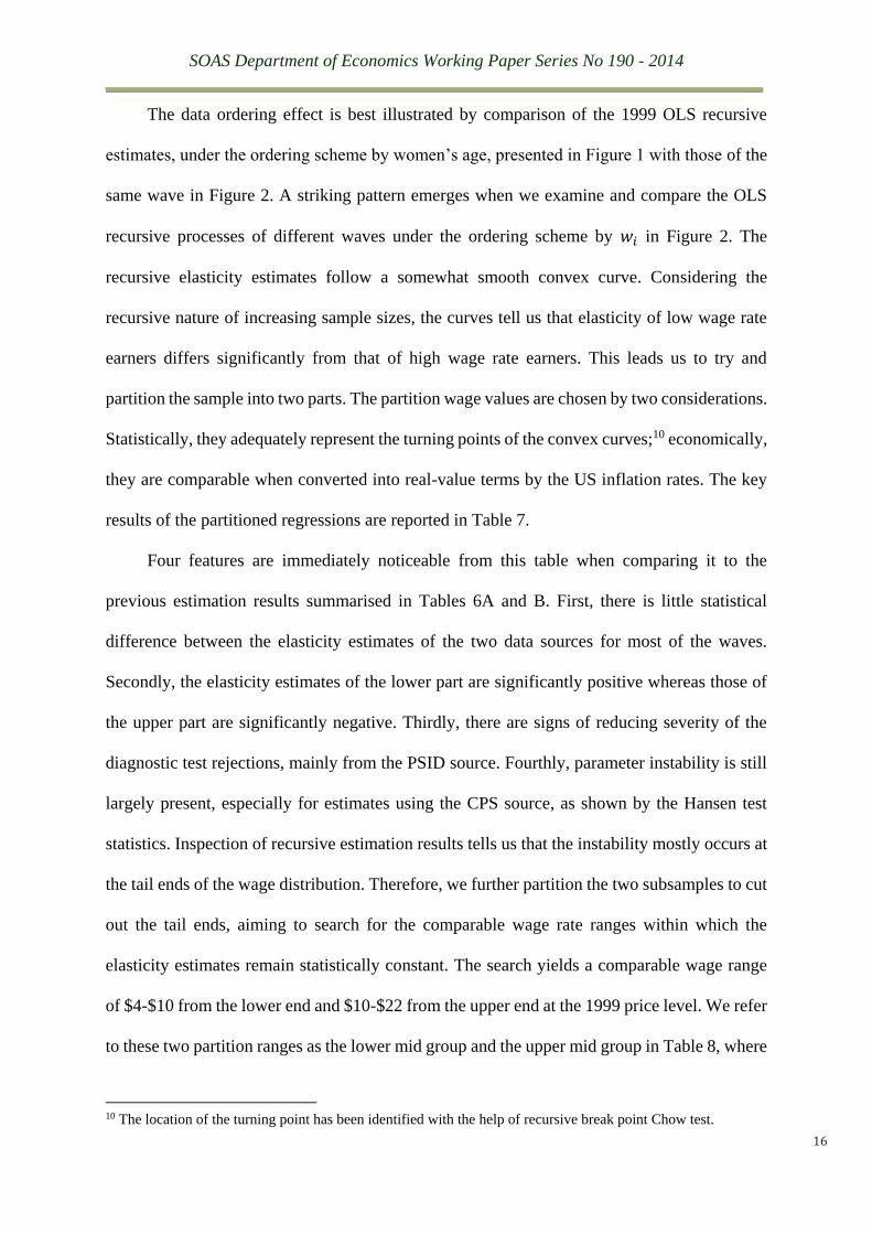
The data ordering effect is best illustrated by comparison of the 1999 OLS recursive
estimates, under the ordering scheme by women’s age, presented in Figure 1 with those of the
same wave in Figure 2. A striking pattern emerges when we examine and compare the OLS
recursive processes of different waves under the ordering scheme by 𝑤𝑖 in Figure 2. The
recursive elasticity estimates follow a somewhat smooth convex curve. Considering the
recursive nature of increasing sample sizes, the curves tell us that elasticity of low wage rate
earners differs significantly from that of high wage rate earners. This leads us to try and
partition the sample into two parts. The partition wage values are chosen by two considerations.
Statistically, they adequately represent the turning points of the convex curves;10 economically,
they are comparable when converted into real-value terms by the US inflation rates. The key
results of the partitioned regressions are reported in Table 7.
Four features are immediately noticeable from this table when comparing it to the
previous estimation results summarised in Tables 6A and B. First, there is little statistical
difference between the elasticity estimates of the two data sources for most of the waves.
Secondly, the elasticity estimates of the lower part are significantly positive whereas those of
the upper part are significantly negative. Thirdly, there are signs of reducing severity of the
diagnostic test rejections, mainly from the PSID source. Fourthly, parameter instability is still
largely present, especially for estimates using the CPS source, as shown by the Hansen test
statistics. Inspection of recursive estimation results tells us that the instability mostly occurs at
the tail ends of the wage distribution. Therefore, we further partition the two subsamples to cut
out the tail ends, aiming to search for the comparable wage rate ranges within which the
elasticity estimates remain statistically constant. The search yields a comparable wage range
of $4-$10 from the lower end and $10-$22 from the upper end at the 1999 price level. We refer
to these two partition ranges as the lower mid group and the upper mid group in Table 8, where
10 The location of the turning point has been identified with the help of recursive break point Chow test.
SOAS Department of Economics Working Paper Series No 190 - 2014
17
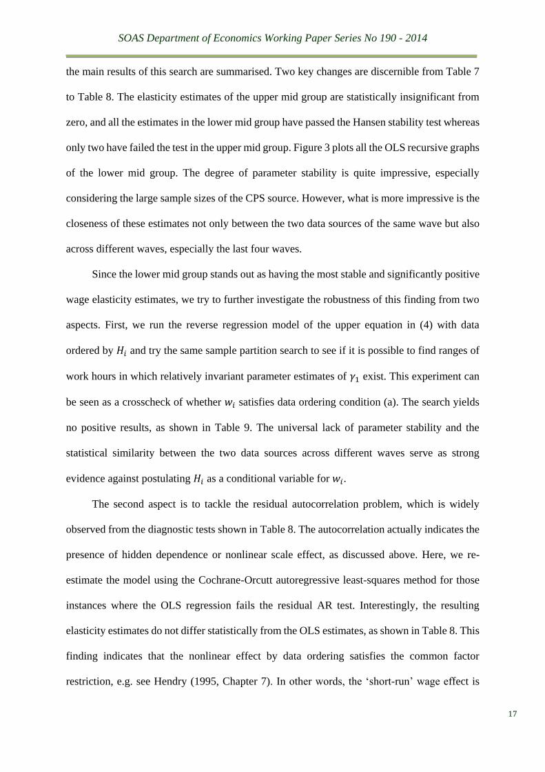
the main results of this search are summarised. Two key changes are discernible from Table 7
to Table 8. The elasticity estimates of the upper mid group are statistically insignificant from
zero, and all the estimates in the lower mid group have passed the Hansen stability test whereas
only two have failed the test in the upper mid group. Figure 3 plots all the OLS recursive graphs
of the lower mid group. The degree of parameter stability is quite impressive, especially
considering the large sample sizes of the CPS source. However, what is more impressive is the
closeness of these estimates not only between the two data sources of the same wave but also
across different waves, especially the last four waves.
Since the lower mid group stands out as having the most stable and significantly positive
wage elasticity estimates, we try to further investigate the robustness of this finding from two
aspects. First, we run the reverse regression model of the upper equation in (4) with data
ordered by 𝐻𝑖 and try the same sample partition search to see if it is possible to find ranges of
work hours in which relatively invariant parameter estimates of 𝛾1 exist. This experiment can
be seen as a crosscheck of whether 𝑤𝑖 satisfies data ordering condition (a). The search yields
no positive results, as shown in Table 9. The universal lack of parameter stability and the
statistical similarity between the two data sources across different waves serve as strong
evidence against postulating 𝐻𝑖 as a conditional variable for 𝑤𝑖.
The second aspect is to tackle the residual autocorrelation problem, which is widely
observed from the diagnostic tests shown in Table 8. The autocorrelation actually indicates the
presence of hidden dependence or nonlinear scale effect, as discussed above. Here, we re-
estimate the model using the Cochrane-Orcutt autoregressive least-squares method for those
instances where the OLS regression fails the residual AR test. Interestingly, the resulting
elasticity estimates do not differ statistically from the OLS estimates, as shown in Table 8. This
finding indicates that the nonlinear effect by data ordering satisfies the common factor
restriction, e.g. see Hendry (1995, Chapter 7). In other words, the ‘short-run’ wage effect is
SOAS Department of Economics Working Paper Series No 190 - 2014
18
identical to the ‘long-run’ wage effect. This is not that surprising considering that the ‘short-
run’ of the present case is wage rate incremental (see Qin and Liu (2013) for more discussion
on this point).
The discovery of statistically constant elasticity estimates in two sub-groups of working
wives not only reconfirms our rejection of models (2) and (4), but also carries a great deal of
practical significance, at least from the following five aspects.
The first and obvious implication of our findings is that wage elasticity for the working
wives is not a single-valued parameter. The evidence from Table 8 that statistically constant
elasticities exist only with respect to certain wage groups undermines the logic foundation of
regarding the labour supply wage effect as a single parameter at the micro, i.e. individual agent
level. Consequently, a theoretical re-orientation is probably needed for those investigations
which are aimed at establishing links between macro and micro labour supply elasticities on
the basis of single-valued micro elasticities. These findings also support more heterodox
theories of labour market segmentation (e.g. Dickens and Lang (1992), Leontaridi (1998)) and
show potential avenues for future empirical research in this field.
Secondly, there is little evidence of dwindling wage elasticities from 1980 to 2011 as far
as those statistically constant elasticities are concerned. On the contrary, these estimates have
remained remarkably invariant, as shown in Table 8. Although some sign of decreasing
elasticities is discernible from the CPS-based estimates of the three waves of 1980, 1990 and
1999, the decrease is statistically too weak to support the claim of dwindling wage elasticities.
If we look at the aggregate estimates from tables 1-6, differences in the wage estimates are
somewhat more noticeable from these three waves. In order to find explanations to this
phenomenon, we look into the share compositions of working wives by our sample partitions.
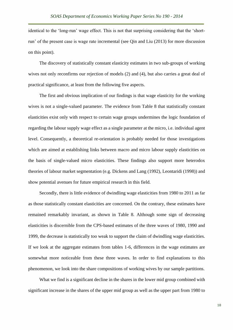
What we find is a significant decline in the shares in the lower mid group combined with
significant increase in the shares of the upper mid group as well as the upper part from 1980 to
SOAS Department of Economics Working Paper Series No 190 - 2014
19
1999, whereas the shares have largely stabilised since 1999, as shown from Figure 4. Since the
lower mid group is the only one where stable and significantly positive elasticities are found to
hold whereas the upper part of the sample contributes to negate the presence of a positive
elasticity, it is no wonder that a dwindling elasticity phenomenon has been observed from
aggregate sample estimations of the 1980-2000 period. This finding tells us that what has
changed over time is not micro elasticities with respect to the lower and upper mid groups, but
the distribution of working wives in relatively lower paid jobs. This is in line with Juhn and
Murphy’s (1997) observation of increasing wage opportunities for women as well as findings
by Welch (2000) on a weakening segregation between male and female labour markets by wage
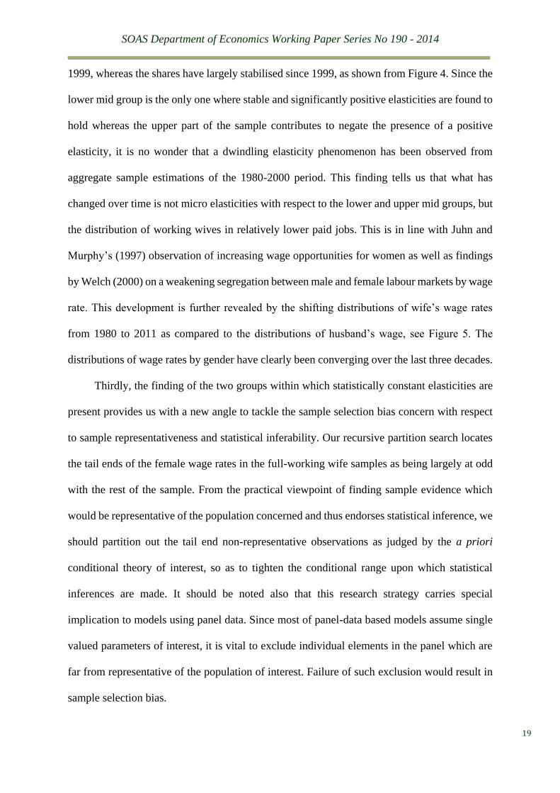
rate. This development is further revealed by the shifting distributions of wife’s wage rates
from 1980 to 2011 as compared to the distributions of husband’s wage, see Figure 5. The
distributions of wage rates by gender have clearly been converging over the last three decades.
Thirdly, the finding of the two groups within which statistically constant elasticities are
present provides us with a new angle to tackle the sample selection bias concern with respect
to sample representativeness and statistical inferability. Our recursive partition search locates
the tail ends of the female wage rates in the full-working wife samples as being largely at odd
with the rest of the sample. From the practical viewpoint of finding sample evidence which
would be representative of the population concerned and thus endorses statistical inference, we
should partition out the tail end non-representative observations as judged by the a priori
conditional theory of interest, so as to tighten the conditional range upon which statistical
inferences are made. It should be noted also that this research strategy carries special
implication to models using panel data. Since most of panel-data based models assume single
valued parameters of interest, it is vital to exclude individual elements in the panel which are
far from representative of the population of interest. Failure of such exclusion would result in
sample selection bias.
SOAS Department of Economics Working Paper Series No 190 - 2014
20
Fourthly, the finding that there is no single-valued wage elasticity across the wage earners
suggests that it could be over-simplistic to treat the non-working wives as a homogenous group
and carry out empirical investigation on aggregate extensive margins by means of binary
regression models. From the viewpoint of measuring wage elasticity for labour participation,
disaggregate studies may be better off partitioning data by wage rate ranges rather than
occupation types. Since our wage imputation method is based on the idea of counterfactual
matching of comparable groups, we can exploit the constant elasticity based sample partitions
to examine how the imputed wage rates are distributed. It is seen from Table 10 that around 70
per cent of non-working wives in the PSID datasets are potentially similar to the lower-mid
group. Results for the CPI samples are somewhat different. While around 60 per cent of the
imputed wage data fall within the lower mid group for the 1980, 1990 and 1999 dataset, this
share drops to 30 per cent for the later waves. Clearly, more experiments are needed to evaluate
the robustness of those imputed wages, but our experiment illustrates how useful the
disaggregate information can be to help better design unemployment policies with respect to
targeting the right groups.
Fifthly, the constant elasticity based sample partitions also provide us with an easy way
to check the necessity or feasibility of grouping data by certain characteristics. For example,
our earlier data ordering scheme by age results in relatively stable elasticity estimates,
indicating it unnecessary to disaggregate data by age groups. In other words, there lacks strong
evidence supporting the hypothesis that different age cohorts have different elasticities. This
check is especially useful for the application of the quantile estimation method. This method
has gained increasing popularity as an intuitively appealing way to tackle heteroscedasticity
and low fit in large micro data sample modelling. The method is based on a conditional quantile
function of interest, a function generally without much a priori theoretical support. In our case,
the method amounts to postulating 𝑄𝜏(𝑙𝑛(𝐻𝑖)|𝑙𝑛(𝑤𝑖), 𝜂𝑤𝜏,∙) as against 𝐸(𝑙𝑛(𝐻𝑖)|𝑙𝑛(𝑤𝑖), 𝜂𝑤,∙),

SOAS Department of Economics Working Paper Series No 190 - 2014
21
which underlies model (1’). Since statistically constant elasticities are found with our two
groups, we can calculate the shares of work hours within these two groups classified by the
four quantiles of 𝐻𝑖 of the working wife sample. The quantile method would be considered
suitable if the shares in one group are dominantly from one quantile. It is clearly seen from
Table 11 that there are no dominant quantiles in either of the two groups to warrant the use of
quantile regressions.
Finally, we try to seek answers to the following question by exploiting the non-unique
ways of data ordering with cross-section data. Do the wives from the two groups have
statistically stable income elasticity? We follow the same strategy as before to try and locate
income ranges within which the recursive estimates of 𝜂𝐼 are statistically constant, when the
full-working women sample estimates turn out to be unstable under the data ordering scheme
by 𝐼𝑖. The key results of the search are reported in Table 12. We then calculate, for the two
wage groups respectively, the shares of the income partitioned by the income ranges reported
in Table 12. We find that the two mid wage groups overlap dominantly with the two mid groups
of the income ranges where constant estimates of 𝜂𝐼 lie, as shown from Table 13. Hence, the
answer to the above question is positive. Moreover, the finding that sizeable shares of income
in both groups fall into the income range where estimates of 𝜂𝐼 are stable but insignificant from
zero helps explain why the estimated income elasticities of these two wage groups are not
highly significant (the details of those estimates are not reported here to keep the paper short).
The above experiment illustrates how versatile the method is to combine data ordering
schemes with recursive partition search for statistically stable estimates of the parameters of
interest. It can help us identify various joint ranges of subgroups from data samples to address
practical questions relating to various compositional issues in compound with the parameters
of interest, in a much more focused and refined manner than aggregate estimation methods.
SOAS Department of Economics Working Paper Series No 190 - 2014
22
4. Concluding Remarks
This project re-examines the commonly used married women’s labour supply model
using six waves of cross-section data from two sources, PSID and CPS, with the intention to
reveal the superfluous the endogeneity-backed IV method and the conventional selection bias
correction for the purpose of estimating wage elasticity with respect to hours of work. Results
of this extensive modelling experiment have not only fulfilled our intension but also revealed
that the superfluousness is not harmless. It actually blocks, by denying the conditional status
of those a priori postulated explanatory variables of interest, the route of systematic data search
to identify the locality where statistically invariant estimates of the parameters of interest hold.
Once the route is unblocked, we are able to make two key discoveries, via extensive use
of recursive techniques combined with various data ordering schemes. Firstly, comparatively
stable and invariant wage elasticity estimates exist only within certain wage ranges over the
last three decades, while secondly, the relative shares of working wives in these ranges have
changed. This change is especially pronounced during the two decades after 1980, whereby
these wage ranges remain remarkably constant in terms of constant-prices. These discoveries
with their locality present to policy makers more reliable and accurate wage elasticity estimates
than what has been available from previous studies. From the viewpoint of academic research,
the power of these discoveries is manifold, as extensively discussed in the previous section. In
short, they help explain the previous finding of dwindling wage elasticity estimates using full
samples of working wives of the CPS source; they invalidate the use of single-valued micro
wage elasticity estimates and also the premise of a single female labour supply market in which
all the housewives are treated as one homogenous group; they provide an easy method to
evaluate the applicability of quantile techniques and also a broader perspective to deal with
sample selection bias than the conventional estimator-based selection bias correction approach.
SOAS Department of Economics Working Paper Series No 190 - 2014
23
There is no need to reiterate the contrasting features between the wage elasticity estimates
presented in Section 3 versus those in Section 2. The wide range of wage parameter estimates
we have produced in Section 2 by following the textbook approach is adequate to show how
arbitrary but fertile the endogeneity-backed IV approach is, thanks to it producing non-optimal
predictors of the explanatory variables of interest which are a priori deemed endogenous.
Widespread paranoia over endogeneity bred by textbook econometrics helps entrap
mainstream micro-econometric research in continuous production of non-unique IV-based
estimates as empirical support for whatever theoretical postulates. The option whether and to
what extent, and/or under what circumstances those postulates could be falsified has been
largely left unexplored. We therefore challenge this IV-based route as ‘playometrics’ (Frisch
1970) because it is far from optimal for scientific discovery.
To a large extent, playometric tools are similar to IVs in that they are apparently
correlated with but not necessarily causally related to the economic issues of concern. The
argument for endogeneity correction on the basis of correlated error terms is a good example,
as discussed in details by Qin (2014a). The use of the Heckman selection bias correction in the
present case is another, as discussed in Section 2. Both cases fall into ‘type III errors’ described
by Kennedy (2002) as far as the empirical question of how to best estimate and verify labour
supply wage elasticity using cross-section survey data is concerned. In other words, both cases
are substantively irrelevant to the empirical question of concern even though they are correct
within the abstract settings where they are presented in textbooks. Sadly, the cost of such
conceptual errors in applied micro-econometric research is substantial in view of the rapid
expansion of data information in contrast to our meagre and sketchy understanding of the data.
It is a widely known fact that model fits usually remain low with large cross-section
survey data samples whatever estimation methods are used. The fact reflects the highly partial
nature of the theories underlying economic models relative to the sample data information. The
SOAS Department of Economics Working Paper Series No 190 - 2014
24
situation thus provides little substantive ground to resort to full-blown SEMs which invoke the
general equilibrium notion. Moreover, large model residuals with rarely fulfilled white-noise
properties call for further criteria to assist model evaluation. For this reason, the invariance
condition of individual parameters of interest is regarded indispensable in the present project.
As shown from our investigation, within sample parameter invariance is predicated on the
choice of data ordering schemes. The non-uniqueness of data ordering schemes provides us
with a fertile laboratory to seek and identify the locality of statistically stable parameter
estimates and also search for hidden dependence in cross-section data. In view of the extensive
theoretical interest in partial derivative based elasticity parameters, data ordering by the
explanatory variable of interest serves as a natural and powerful tool in bridging theory and
data. Obviously, such data ordering assumes the explanatory variable of interest under concern
to be a ‘fixed’ regressor, i.e. a valid conditional or exogenous variable. Once we step out of the
textbook straitjacket of ‘endogeneity bias’ we can better appreciate the role of a priori theories.
They are seldom proved wrong in postulating key conditional variables but are frequently
inadequate or incomplete in specifying either the functional form or other auxiliary explanatory
variables necessary due to various special circumstances of the data samples under
consideration. It is a strategic mistake to tamper with the incompleteness by modifying the
conditional status of those key variables.
It should be noted that our discovery is essentially based on the OLS, a method rigorously
banished for limited dependent models in textbook micro-econometrics. The history of macro-
econometrics shows us that it takes over two decades for the profession to shake off the
endogeneity paranoia from around 1960, when adequate empirical evidence was first presented
to resurrect OLS. It is clearly a huge challenge to initiate a similar resurrection in micro-
econometrics. Hopefully, applied micro modellers can overcome the endogeneity paranoia
sooner than twenty years, with the help of the rapidly growing data availability and data
SOAS Department of Economics Working Paper Series No 190 - 2014
25
processing technology (see Angrist and Pischke (2010)) as well as the lessons learned from the
history of macro-econometrics.
Clearly, much refinement is desired of our current results and also methods of
investigation. An obvious next step is the analysis of husband’s wage elasticity using the same
set of data to compare whether the heterogeneity found for the wife’s samples also holds for
the husbands’ samples. Further, more experiments with the wage imputation methods are
desired and ways should be explored as how to utilise disaggregate wage range groups to
conduct disaggregate studies of the wage elasticities of labour force participation in a
comparable manner with those of the hours of work. Last but not least, adaption of more
systematic data mining techniques is desired, especially from recent developments in statistics
into micro-econometrics, such as the method of model-based recursive partition (see Kopf et
al (2013)). Hopefully, such adaptions would lead to new avenues in microeconomic research.

SOAS Department of Economics Working Paper Series No 190 - 2014
26
Appendix 1. Data processing
Two USA based cross-sectional data sources have been taken into consideration, which are the
March Annual Demographic Survey of the Current Population Survey (CPS) published by the
Bureau of Labor Statistics, United States Department of Labor and the Panel Study of Income
Dynamics (PSID) conducted by the Survey Research Centre at the University of Michigan. For
the CPS data the Center for Economic and Policy Research (CEPR) Uniform Extracts are used.
From both datasets the following variables have been extracted: wife’s annual hours of work,
wife’s hourly wage rate, family income net of wife’s income, wife’s education, wife’s age,
husband’s annual hours of work, husband’s hourly wage rate, husband’s education, husband’s
age, a dummy which takes on 1 if children under 6 are in the household and 0 otherwise, and
the number of children in the household. For the CPS data and additional dummy variable for
the wife’s ethnical background is included; for the PSID data a variable for wife’s experience
is used, which is not available in the CPS data source.
Following Heim (2007) and Blau and Kahn (2007) the annual hours worked variable in CPS is
created by multiplying the usual hours worked per week times the number of weeks worked in
the past calendar year. Regarding the hourly wage rate, we follow Heim (2007) in using the
hourly wage rate as reported if available and if the wage per week is reported, this is divided
by the usual hours worked per week. For the education variable the coding suggested by the
CPS March Codebook for item 18h is used. For family income net wife’s income, the wife’s
personal income from wages and salaries (hourly wage rate times annual hours) is subtracted
from total family income.
Both CPS and PSID data sets are processed by the following selection criteria.
- Exclude if woman is non-married, divorced, widowed or separated.
- Include only women with age range 25 to 60.
- Exclude if husband is not working (0 wage).
- Exclude if missing data on wife’s education.
- Exclude if missing data on husband’s education.
- Exclude if wife’s annual working hours exceed 4000.
- Exclude if husband’s annual working hours exceed 4000.
- Exclude if wife’s wage rate exceeds $300 USD or is below $1 USD at 1999 price level
per hour.
- Exclude if husband’s wage rate exceeds $300 USD or is below $1 USD at 1999 price
level per hour.
- Exclude if total family income net of wife’s income is smaller than 0.
- Exclude if wife has reported positive working hours but no wage and vice versa.
Table A1 provides detailed summary statistics of the different waves for the two datasets.
Appendix 2. Imputation Method
SOAS Department of Economics Working Paper Series No 190 - 2014
27
The missing wage rates are imputed by the hot deck method, e.g. see Little and Vartivarian
(2005), Andridge and Little (2010). The method derives each missing value, referred to as a
recipient, from a few donors who are found to share similar characteristics with the recipient.
The method consists of the following two steps.
Step 1: Establish a metric for matching donors to recipients. The purpose of the metric is to
produce one summary measure comparable between the recipients and the donors. The metric
used here is a multiple regression of the upper equation of (2) using the working wife sample
only. Several regressions have been experimented with various choices of regressors and the
selected model must have all the regressors with statistically stable parameters. The fitted
wages are then calculated as representing the summary measures of the donors. The fitted
model is used to ‘predict’ a series of the summary measures of all the recipients. We have also
tried the alternative of running a binary model, i.e. a labour force participation model, using
the full sample including the non-working wives, with the aim to use the fitted probability
scores for the 2nd step matching. However, it is difficult to assess how invariant the estimated
coefficients and thus how credible the ‘predicted’ probability scores are. The trial matched
results tend to be smoother than those by the OLS regression metric, making the imputed
missing wage rates appear less similar to the observed wage rates, as compared to those
imputed by the OLS regression metric. We have therefore abandoned this binary regression
metric.
Step 2: Match recipients with their closest neighbours by their summary measures from step 1.
This is done by a combination of the nearest-neighbour matching method and the radius
matching method. Specifically, we set a starting radius to search for a set number of donors
from the lower end of the wage scale (the number is set at five here, in line with what is
commonly used in the programme evaluation matching literature). For those recipients which
have not yet got enough donors, we gradually enlarge the radius until the required number of
donors are found. The missing wage value of a recipient is taken as the average of the observed
wage rates of the donors.
Acknowledgments
We would like to thank Machiko Nissanke, Ron Smith, Achim Zeileis, Andrey Kuleshov, and
Lifong Zou for their invaluable help and support.
SOAS Department of Economics Working Paper Series No 190 - 2014
28
References
Andridge, R. R., and Little, R. J. (2010). A Review of Hot Deck Imputation for Survey Non-
response. International Statistical Review, 78(1), 40-64.
Angrist, J. D., and Krueger, A. B. (1999). Empirical Strategies in Labour Economics. In O.
Ashenfelter, and D. C. (eds.), Handbook of Labor Economics, Vol. III (pp. 1278-
1366). New York: North-Holland.
Angrist, J., and Pischke, J.-S. (2010). The Credibility Revolution in Empirical Economics:
How Better Research Design is Taking the Con out of Econometrics. NBER:
Working Paper, No. 15794.
Berndt, E. R. (1991). The Practice of Econometrics: Classic and Contemporary. Addison
Wesley.
Blau, F. D., and Kahn, L. M. (2007). Changes in the Labor Supply Behaviour of Married
Women: 1980-2000. Journal of Labor Economics, 25, 393-438.
Blundell, R., and MaCurdy, T. (1999). Labor Supply: A Review of Alternative Approaches.
In O. Ashenfelter, and D. C. (ed.), Handbook of Labor Economics, Vol. III (pp.
1559-1695). New York: North-Holland.
Bound, J., Jaeger, D. A., and Baker, R. M. (1995). Problems With Instrumental Variables
Estimation When the Correlation Between the Instruments and the Endogeneous
Explanatory Variable is Weak. Journal of the American Statistical Association,
90(430).
Cetty, R., Guren, A., Manoli, D., and Weber, A. (2011). Are Micro and Macro Labor Supply
Elasticities Consistent? A Review of Evidence on the Intensive and Extensive
Margins. American Economic Review, 101(3), 471-475.
Chung, C.-F., and Goldberger, A. S. (1984). Proportional Projections in Limited Dependent
Variable Models. Econometrica, 52(2), 531-534.
Dickens, W. T., and Lang, K. (1992). Labor Market Segmentation Theory: Reconsidering the
Evidence. NBER: Working Paper, No. 4087.
Eika, L., Mogstad, M., and Zafar, B. (2014). Educational Assortative Mating and Household
Income Inequality. NBER: Working Paper, No. 20271.
Fiorito, R., and Zanella, G. (2012). The Anatomy of the Aggregate Labor Supply Elasticity.
Review of Economic Dynamics, 15, 171-187.
Frisch, R. (1970). Econometrics in the World of Today. In W. Eltis, M. F. Scott, J. N. Wolfe,
and S. R. (eds.), Induction, Growth and Trade: Essays in Honour of Sir Roy Harrod
(pp. 153-166). Oxford: Clarendon Press.
SOAS Department of Economics Working Paper Series No 190 - 2014
29
Gersuny, C. (1982). Employment Seniority: Cases From lago to Weber. Journal of Labour
Research, 3(1), 111-119.
Goldin, C. (1990). Understanding the Gender Gap. New York : Oxford University Press.
Greene, W. H. (1981). On the Asymptotic Bias of the Ordinary Least Squares Estimator.
Econometrica, 49(2), 505-513.
Heckman, J. J. (1976). A Life-cycle Model of Earnings, Learning, and Consumption. Journal
of Political Economy, 84(4), 11-44.
Heckman, J. J. (1979). Sample Selection Bias as a Specification Error. Econometrica, 47(1),
153-161.
Heckman, J. J. (1993). What Has been Learned About Labor Supply in the Past Twenty
Years? The American Economic Review, 83(2), 116-121.
Heim, B. T. (2007). The Incredible Shrinking Elasticities: Married Female Labor Supply,
1978–2002. Journal of Human Resources, 42, 881-918.
Hendry, D. F. (1995). Dynamic Econometrics. Oxford: Oxford University Press.
Hendry, D. F. (2009). The Methodology of Empirical Econometric Modeling: Applied
Econometrics Through the Looking-Glass. In T. C. Mills, and K. D. Patterson,
Palgrave Handbook of Econometrics, Volume 2: Applied Econometrics (pp. 3-67).
Palgrave MacMillan.
Juhn, C., and Murphy, K. M. (1997). Wage Inequality and Family Labor Supply. Journal of
Labor Economics, 15(1), 72-97.
Keane, M., and Rogerson, R. (2012). Micro and Macro Labor Supply Elasticities: A
Reassessment of Conventional Wisdom. Journal of Economic Literature, 50(2), 464-
476.
Kennedy, P. E. (2002). Sinning in the Basement: What are the Rules? The Ten
Commandments if Applied Econometrics. Journal of Economic Surveys, 16(4), 569-
589.
Killingsworth, M. R. (1983). Labour Supply. Cambridge: Cambridge University Press.
Killingsworth, M. R., and Heckman, J. J. (1986). Female Labor Supply: A Survey. In O.
Ashenfelter, and R. L. (ed.), Handbook of Labor Economics, Vol. I (pp. 103-204).
New York: North-Holland.
Kopf, J., Augustin, T., and Strobl, C. (2013). The Potential of Model-based Recursive
Partitioning in the Social Sciences – Revisiting Ockham’s Razor. In J. McArdle, and
G. R. (eds.), Contemporary Issues in Exploratory Data Mining (pp. 75-95). New
York and London: Routledge.
SOAS Department of Economics Working Paper Series No 190 - 2014
30
Leontaridi, M. (1998). Segmented Labour Markets: Theory and Evidence. Journal of
Economic Surveys, 12(1), 103-109.
Little, R. J., and Vartivarian, S. (2005). Does Weighting for Nonresponse Increase the
Variance of Survey Means? Survey Methodology, 31, 161-168.
McClelland, R., and Mok, S. (2012). A Review of Recent Research on Labor Supply
Elasticities. Congressional Budget Office: Working Paper 2012-12,
https://www.cbo.gov/publication/43675.
Merkle, E. C., Fan, J., and Zeileis, A. (2013). Testing for Measurement Invariance with
Respect to an Ordinal Variable . Psychometrika, 1-16.
Mincer, J. (1962). Labour Force Participation of Married Women: A Study of Labour Supply.
In H. G. (ed.), Aspects of Labour Economics (pp. 9-41). Princeton: Princeton
University Press.
Moffitt, R. A. (1999). New Developments in Econometric Methods for Labor Market
Analysis. In O. Ashenfelter, and D. C. (eds.), Handbook of Labor Economics, Vol.
III (pp. 1368-1397). New York: North-Holland.
Mroz, T. A. (1987). The Sensitivity of an Empirical Model of Married Women's Hours of
Work to Economic and Statistical Assumptions. Econometrica, 55(4), 765-799.
Newey, W. K., Powell, J. L., and Walker, J. R. (1990). Semiparametric Estimation of
Selection Models: New Results. American Economic Review, 80(2), 324-328.
Olsen, R. J. (1980). A Least Squares Correction for Selectivity Bias. Econometrica, 48(7),
1815-1820.
Pagan, A., and Vella, F. (1989). Diagnostic Test for Models Based on Individual Data: A
Survey. Journal of Applied Econometrics, 4 (Supplement: Special Issue on Topics in
Applied Econometrics), 29-59.
Perron, P., and Yamamoto, Y. (2013). Using OLS to Estimate and Test for Structural
Changes in Models with Endogenous Regressors . Journal of Applied Econometrics,
doi: 10.1002/jae.2320.
Peterman, W. B. (2014). Reconciling Micro and Macro Estimates of the Frisch Labor Supply
Elasticity: A Sensitivity Analysis. Federal Reserve Board of Governors: Working
Paper July 2014.
Puhani, P. (2000). The Heckman Correction for Sample Selection and Its Critique. Journal of
Economic Surveys, 14(1), 53-68.
Qin, D. (1993). Formation of Econometrics: A Historical Perspective. Oxford: Oxford
University Press.
SOAS Department of Economics Working Paper Series No 190 - 2014
31
Qin, D. (2013). A History of Econometrics: The Reformation from the 1970s. Oxford:
Oxford University Press.
Qin, D. (2014a). Resurgence of Instrument Variable Estimation and Fallacy of Endogeneity.
Kiel Institute for the World Economy: Economics Discussion Papers, No 2014-42,
http://www.economics-ejournal.org/economics/discussionpapers/2014-42.
Qin, D. (2014b). Inextricability of Autonomy and Confluence in Econometrics. Oeconomia,
4(3), 321-341.
Qin, D., and Liu, Y. (2013). Modelling Scale Effect in Cross-section Data: The Case of
Hedonic Price Regression. SOAS Department of Economics: Working Paper Series,
No. 184.
Rupert, P., and Zanella, G. (2014). Revisiting Wage, Earnings, and Hours Profiles.
Dipartimento Scienze Economiche, Universita' di Bologna: Working Paper, Nr. 936 .
Sims, C. A. (1980). Macroeconomics and Reality. Econometrica, 48(1), 1-48.
Welch, F. (2000). Growth in Women's Relative Wages and in Inequality among Men: One
Phenomenon or Two? The American Economic Review, 90(2), Papers and
Proceedings of the One Hundred Twelfth Annual Meeting of the American
Economic Association, 444-449.
Zeileis, A., and Hornik, K. (2007). Generalized M-fluctuation Tests for Parameter Instability.
Statistica Neerlandica, 61(4), 488-508.
SOAS Department of Economics Working Paper Series No 190 - 2014
32
Table 1. IV estimates of 𝛼1 in model (2) and related statistics, working wife samples
Calibration case Blau and Kahn (2007, Model 4, Table 6) Heim (2007, Table 1)
CPS PSID PSID CPS PSID PSID
IVs Set 1 Set 2 Set 3 Set 4
1980
Target �̂�1𝐼𝑉 ≈ 366.4 = 0.252 ∗ 1454 �̂�1
𝐼𝑉 = 533.7, 95% C.I.(-128.7, 1196.1)
�̂�1𝐼𝑉 314.294** -166.399 222.999** 332.244** -166.98* 295.2**
95% C.I. (232.9, 395.7) (-333.3, 0.47) (62.4, 383.6) (251.1, 413.4) (-333, -1.2) (130.4, 460)
Hausman 17.6683** 16.8924** 1.4593 21.9117** 17.0288** 4.692*
1st adj.𝑅2 0.1164 0.1929 0.1809 0.1181 0.1933 0.1740
Over-id. 118.26** 17.8094** 75.4455** 139.099** 17.8187** 65.307**
Elasticity 0.2095 -0.1109 0.1487 0.2215 -0.1113 0.1968
1990
Target �̂�1𝐼𝑉 ≈ 352.7 = 0.216 ∗ 163 �̂�1
𝐼𝑉 = 534, 95% C.I.(124.8, 943.2)
�̂�1𝐼𝑉 317.371** 79.63 328.29** 318.2681** 68.339 385.93**
95% C.I. (265.2, 369.5) (-15.1, 174.3) (223.6, 423) (266.2, 370.3) (-26.1, 162.8) (286.9, 484.9)
Hausman 15.331** 5.8480* 13.125** 15.664** 7.3365** 23.437**
1st adj.𝑅2 0.1987 0.2618 0.2415 0.1983 0.2648 0.2286
Over-id. 78.558** 19.8407** 68.957** 86.5651** 23.6909** 63.578**
Elasticity 0.2116 0.0531 0.219 0.2122 0.0456 0.2573
1999
Target �̂�1𝐼𝑉 ≈ 213.3 = 0.122 ∗ 1748 �̂�1
𝐼𝑉 = 303.7, 95% C.I.(-161.3, 768.7)
�̂�1𝐼𝑉 259.362** 82.727 221.75** 262.9916** 81.3817 267.82**
95% C.I. (209.2, 309.6) (-30.6, 196.1) (111, 332.5) (212.9, 313.1) (-31.99, 194.8) (149.1, 386.5)
Hausman 22.2944** 0.4613 4.4123* 23.8535** 0.4989 7.364**
1st adj.𝑅2 0.2078 0.2320 0.2194 0.2080 0.2317 0.2177
Over-id. 84.886** 31.3218** 30.717** 91.9335** 32.548** 14.137**
Elasticity 0.1729 0.0552 0.1478 0.1753 0.0543 0.1785
2003
�̂�1𝐼𝑉 207.1** 172.87** 314.07** 207.741** 177.3855** 344.115**
95% C.I. (169.3, 245) (35.2, 310.5) (178.2, 449.9) (170.0, 245.5) (42.6, 312.2) (200.3, 488)
Hausman 22.567** 3.6356 19.1** 22.935** 4.0707* 23.138**
1st adj.𝑅2 0.2164 0.2001 0.1823 0.2038 0.1998 0.1806
Over-id. 168.77** 19.609** 19.753** 170.089** 19.7775** 13.0213**
Elasticity 0.1381 0.1152 0.2094 0.1395 0.1183 0.2294
2007
�̂�1𝐼𝑉 178.55** 92.669 217.796** 178.267** 86.893 296.759**
95% C.I. (142, 215.1) (-20.7, 206) (96.88, 338.7) (141.8, 214.8) (-25.9, 199.7) (162.9, 430.7)
Hausman 9.5622** 0.018 5.923* 9.4702** 0.0005 13.32**
1st adj.𝑅2 0.2203 0.2289 0.1862 0.2122 0.2288 0.1754
Over-id. 155.41** 26.182** 47.478** 155.672** 26.432** 32.734**
Elasticity 0.119 0.0618 0.1452 0.1188 0.0579 0.1978
2011
�̂�1𝐼𝑉 292.8** 331.814** 423.402** 292.306** 335.46** 437.553
95% C.I. (255.8, 330) (202.4, 461) (288.9, 557.9) (255.3, 329.3) (206, 464.9) (300.1, 575)
Hausman 68.682** 11.234** 23.28** 68.682** 11.7021** 25.19**
1st adj.𝑅2 0.2451 0.1849 0.1618 0.2282 0.1848 0.1681
Over-id. 111.62** 7.9784 29.226** 113.109** 9.1695 26.2**
Elasticity 0.1952 0.2212 0.2823 0.1949 0.2236 0.2917
Note: C.I. stands for confidence interval; Hausman is the Wu-Hausman test of endogeneity; Over-id. stands for Sargan over-identification tests; ** and * indicate significance at 1% and 5% respectively. 1st adj.𝑅2 stands for adjusted 𝑅2 of the first stage regression from the 2SLS/IV procedure; IV set 1: Husband’s education, husband’s wage rate in log, wife’s education, wife’s education in quadratic and cubic forms. IV set 2: Wife’s education, its quadratic and cubic forms, wife’s previous years of work, wife’s age in cubic form. IV set 3: Same IVs as in Set 1 plus inverse Mill’s ratio conditional on family non-wife income in log, wife’s education, wife’s age in cubic, number of children, presence of children under 6. IV set 4: Wife’s education, wife’s previous years of work, wife’s age in cubic form and the same inverse Mill’s ratio as in Set 3. Elasticity is evaluated at 1500 hours.
SOAS Department of Economics Working Paper Series No 190 - 2014
33
Table 2. IV tobit estimates of 𝛼1 in model (2) and related statistics using the same IV sets as in
Table 1, full samples including non-working wives
CPS PSID PSID CPS PSID PSID
IVs Set 1 Set 2 Set 3 Set 4
1980
�̂�1𝐼𝑉 1103.22 722.38 1260.62 1162.553 734.9121 1408.975
95% C.I. (1038,1169) (529.2,915.6) (1070,1451) (1099,1226) (541.7,928.1) (1204,1614)
Wald 18.99** 3.14 80.16** 6.21* 3.83 103.36**
Over-id. 297.854** 34.789** 152.895** 353.823** 48.346** 121.252**
1990
�̂�1𝐼𝑉 768.3579 596.1497 1090.07 777.22 600.07 1246.528
95% C.I. (730.0,806.7) (481.8,710.6) (980.8,1199) (739.2,815.2) (486.1,714.1) (1128,1365)
Wald 91.83** 0.54 112.53** 83.67** 0.43 172.53**
Over-id. 225.775** 77.268** 266.414** 237.921** 77.815** 165.987**
1999
�̂�1𝐼𝑉 674.6063 508.9325 784.589 680.8055 515.2407 930.1164
95% C.I. (637.4,711.9) (371.6,646.3) (647.7,921.5) (643.7,717.9) (378,652.5) (782.4,1078)
Wald 89.34** 0.02 23.91** 83.08** 0.07 46.72**
Over-id. 175.907** 66.341** 115.620** 187.119** 68.125** 64.593**
2003
�̂�1𝐼𝑉 626.9265 492.3992 763.7196 627.5508 517.1577 864.2152
95% C.I. (598.1,655.7) (338,646.8) (614.1,913.4) (598.7,656.4) (364.7,669.7) (705.5,1023)
Wald 169.57** 0.00 16.64** 167.73** 0.11 27.80**
Over-id. 384.788** 28.452** 71.022** 386.904** 32.104** 48.613**
2007
�̂�1𝐼𝑉 624.1504 485.6784 677.1806 623.2197 485.0906 851.3809
95% C.I. (597.0,651.3) (348.3,623.0) (534.1,820.3) (596,650.5) (349.6,620.6) (691.9,1011)
Wald 159.96** 0.01 9.45** 161.11** 0.01 26.88**
Over-id. 448.117** 54.741** 99.299** 447.535** 54.743** 59.157**
2011
�̂�1𝐼𝑉 645.2837 850.8864 1004.48 644.3989 860.8814 1047.094
95% C.I. (619.6,671.0) (701.9,999.9) (852.5,1157) (618.7,670.1) (711.8,1010) (890,1204.2)
Wald 143.01** 11.13** 31.44** 144.24** 12.36** 36.83**
Over-id. 238.034** 31.499** 48.468** 238.488** 36.007** 39.539**
Note: C.I. stands for confidence interval; Wald is the Wald test of exogeneity; Over-id. stands for Sargan over-identification tests; ** and * indicate significance at 1% and 5% respectively. IV sets are identical to those in Table 1. Elasticity is evaluated at 1500 hours.
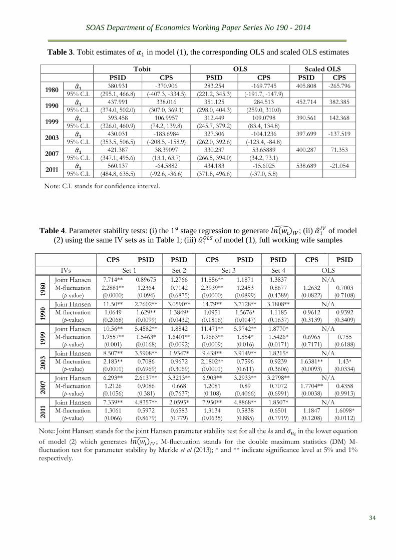
SOAS Department of Economics Working Paper Series No 190 - 2014
34
Table 3. Tobit estimates of 𝛼1 in model (1), the corresponding OLS and scaled OLS estimates
Tobit OLS Scaled OLS PSID CPS PSID CPS PSID CPS
1980 �̂�1 380.931 -370.906 283.254 -169.7745 405.808 -265.796
95% C.I. (295.1, 466.8) (-407.3, -334.5) (221.2, 345.3) (-191.7, -147.9)
1990 �̂�1 437.991 338.016 351.125 284.513 452.714 382.385
95% C.I. (374.0, 502.0) (307.0, 369.1) (298.0, 404.3) (259.0, 310.0)
1999 �̂�1 393.458 106.9957 312.449 109.0798 390.561 142.368
95% C.I. (326.0, 460.9) (74.2, 139.8) (245.7, 379.2) (83.4, 134.8)
2003 �̂�1 430.031 -183.6984 327.306 -104.1236 397.699 -137.519
95% C.I. (353.5, 506.5) (-208.5, -158.9) (262.0, 392.6) (-123.4, -84.8)
2007 �̂�1 421.387 38.39097 330.237 53.65889 400.287 71.353
95% C.I. (347.1, 495.6) (13.1, 63.7) (266.5, 394.0) (34.2, 73.1)
2011 �̂�1 560.137 -64.5882 434.183 -15.6025 538.689 -21.054
95% C.I. (484.8, 635.5) (-92.6, -36.6) (371.8, 496.6) (-37.0, 5.8)
Note: C.I. stands for confidence interval.
Table 4. Parameter stability tests: (i) the 1st stage regression to generate 𝑙𝑛(𝑤𝑖)̂𝐼𝑉; (ii) �̂�1
𝐼𝑉 of model
(2) using the same IV sets as in Table 1; (iii) �̂�1𝑂𝐿𝑆 of model (1), full working wife samples
CPS PSID PSID CPS PSID PSID CPS PSID
IVs Set 1 Set 2 Set 3 Set 4 OLS
1980 Joint Hansen 7.714** 0.89675 1.2766 11.856** 1.1871 1.3837 N/A
M-fluctuation (p-value)
2.2881** (0.0000)
1.2364 (0.094)
0.7142 (0.6875)
2.3939** (0.0000)
1.2453 (0.0899)
0.8677 (0.4389)
1.2632 (0.0822)
0.7003 (0.7108)
1990 Joint Hansen 11.50** 2.7602** 3.0590** 14.79** 3.7128** 3.1808** N/A
M-fluctuation (p-value)
1.0649 (0.2068)
1.629** (0.0099)
1.3849* (0.0432)
1.0951 (0.1816)
1.5676* (0.0147)
1.1185 (0.1637)
0.9612 (0.3139)
0.9392 (0.3409)
1999 Joint Hansen 10.56** 5.4582** 1.8842 11.471** 5.9742** 1.8770* N/A
M-fluctuation (p-value)
1.9557** (0.001)
1.5463* (0.0168)
1.6401** (0.0092)
1.9663** (0.0009)
1.554* (0.016)
1.5426* (0.0171)
0.6965 (0.7171)
0.755 (0.6188)
2003 Joint Hansen 8.507** 3.5908** 1.9347* 9.438** 3.9149** 1.8215* N/A
M-fluctuation (p-value)
2.183** (0.0001)
0.7086 (0.6969)
0.9672 (0.3069)
2.1802** (0.0001)
0.7596 (0.611)
0.9239 (0.3606)
1.6381** (0.0093)
1.43* (0.0334)
2007 Joint Hansen 6.293** 2.6137** 3.3213** 6.903** 3.2933** 3.2798** N/A
M-fluctuation (p-value)
1.2126 (0.1056)
0.9086 (0.381)
0.668 (0.7637)
1.2081 (0.108)
0.89 (0.4066)
0.7072 (0.6991)
1.7704** (0.0038)
0.4358 (0.9913)
2011
Joint Hansen 7.339** 4.8357** 2.0595* 7.950** 4.8868** 1.8507* N/A
M-fluctuation (p-value)
1.3061 (0.066)
0.5972 (0.8679)
0.6583 (0.779)
1.3134 (0.0635)
0.5838 (0.885)
0.6501 (0.7919)
1.1847 (0.1208)
1.6098* (0.0112)
Note: Joint Hansen stands for the joint Hansen parameter stability test for all the λs and 𝜎𝑢𝑖 in the lower equation
of model (2) which generates 𝑙𝑛(𝑤𝑖)̂𝐼𝑉 ; M-fluctuation stands for the double maximum statistics (DM) M-
fluctuation test for parameter stability by Merkle et al (2013); * and ** indicate significance level at 5% and 1% respectively.
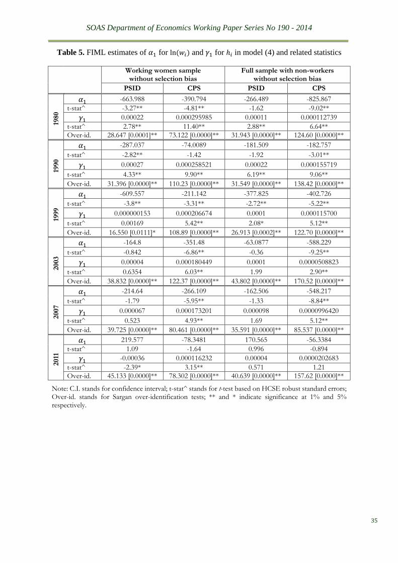
SOAS Department of Economics Working Paper Series No 190 - 2014
35
Table 5. FIML estimates of 𝛼1 for ln (𝑤𝑖) and 𝛾1 for ℎ𝑖 in model (4) and related statistics
Working women sample
without selection bias Full sample with non-workers
without selection bias
PSID CPS PSID CPS
1980
𝛼1 -663.988 -390.794 -266.489 -825.867
t-stat^ -3.27** -4.81** -1.62 -9.02**
𝛾1 0.00022 0.000295985 0.00011 0.000112739
t-stat^ 2.78** 11.40** 2.88** 6.64**
Over-id. 28.647 [0.0001]** 73.122 [0.0000]** 31.943 [0.0000]** 124.60 [0.0000]**
1990
𝛼1 -287.037 -74.0089 -181.509 -182.757
t-stat^ -2.82** -1.42 -1.92 -3.01**
𝛾1 0.00027 0.000258521 0.00022 0.000155719
t-stat^ 4.33** 9.90** 6.19** 9.06**
Over-id. 31.396 [0.0000]** 110.23 [0.0000]** 31.549 [0.0000]** 138.42 [0.0000]**
1999
𝛼1 -609.557 -211.142 -377.825 -402.726
t-stat^ -3.8** -3.31** -2.72** -5.22**
𝛾1 0.000000153 0.000206674 0.0001 0.000115700
t-stat^ 0.00169 5.42** 2.08* 5.12**
Over-id. 16.550 [0.0111]* 108.89 [0.0000]** 26.913 [0.0002]** 122.70 [0.0000]**
2003
𝛼1 -164.8 -351.48 -63.0877 -588.229
t-stat^ -0.842 -6.86** -0.36 -9.25**
𝛾1 0.00004 0.000180449 0.0001 0.0000508823
t-stat^ 0.6354 6.03** 1.99 2.90**
Over-id. 38.832 [0.0000]** 122.37 [0.0000]** 43.802 [0.0000]** 170.52 [0.0000]**
2007
𝛼1 -214.64 -266.109 -162.506 -548.217
t-stat^ -1.79 -5.95** -1.33 -8.84**
𝛾1 0.000067 0.000173201 0.000098 0.0000996420
t-stat^ 0.523 4.93** 1.69 5.12**
Over-id. 39.725 [0.0000]** 80.461 [0.0000]** 35.591 [0.0000]** 85.537 [0.0000]**
2011
𝛼1 219.577 -78.3481 170.565 -56.3384
t-stat^ 1.09 -1.64 0.996 -0.894
𝛾1 -0.00036 0.000116232 0.00004 0.0000202683
t-stat^ -2.39* 3.15** 0.571 1.21
Over-id. 45.133 [0.0000]** 78.302 [0.0000]** 40.639 [0.0000]** 157.62 [0.0000]**
Note: C.I. stands for confidence interval; t-stat^ stands for t-test based on HCSE robust standard errors; Over-id. stands for Sargan over-identification tests; ** and * indicate significance at 1% and 5% respectively.
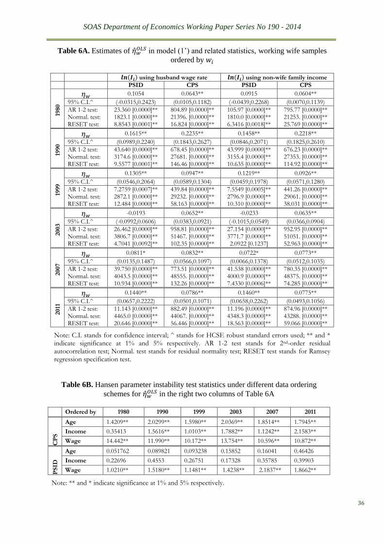
SOAS Department of Economics Working Paper Series No 190 - 2014
36
Table 6A. Estimates of �̂�𝑤𝑂𝐿𝑆 in model (1’) and related statistics, working wife samples
ordered by 𝑤𝑖
𝒍𝒏(𝑰𝒊) using husband wage rate 𝒍𝒏(𝑰𝒊) using non-wife family income
PSID CPS PSID CPS
1980
𝜂𝑤 0.1054 0.0643** 0.0915 0.0604**
95% C.I.^ (-0.0315,0.2423) (0.0105,0.1182) (-0.0439,0.2268) (0.0070,0.1139)
AR 1-2 test: Normal. test: RESET test:
23.360 [0.0000]** 1823.1 [0.0000]** 8.8543 [0.0001]**
804.89 [0.0000]** 21396. [0.0000]** 16.824 [0.0000]**
105.97 [0.0000]** 1810.0 [0.0000]** 6.3416 [0.0018]**
795.77 [0.0000]** 21253. [0.0000]** 25.769 [0.0000]**
1990
𝜂𝑤 0.1615** 0.2235** 0.1458** 0.2218**
95% C.I.^ (0.0989,0.2240) (0.1843,0.2627) (0.0846,0.2071) (0.1825,0.2610)
AR 1-2 test: Normal. test: RESET test:
43.640 [0.0000]** 3174.6 [0.0000]** 9.5577 [0.0001]**
678.45 [0.0000]** 27681. [0.0000]** 146.46 [0.0000]**
43.999 [0.0000]** 3155.4 [0.0000]** 10.635 [0.0000]**
676.23 [0.0000]** 27353. [0.0000]** 114.92 [0.0000]**
1999
𝜂𝑤 0.1305** 0.0947** 0.1219** 0.0926**
95% C.I.^ (0.0546,0.2064) (0.0589,0.1304) (0.0459,0.1978) (0.0571,0.1280)
AR 1-2 test: Normal. test: RESET test:
7.2759 [0.0007]** 2872.1 [0.0000]** 12.484 [0.0000]**
439.84 [0.0000]** 29232. [0.0000]** 58.163 [0.0000]**
7.5549 [0.0005]** 2796.9 [0.0000]** 10.310 [0.0000]**
441.26 [0.0000]** 29061. [0.0000]** 38.031 [0.0000]**
2003
𝜂𝑤 -0.0193 0.0652** -0.0233 0.0635**
95% C.I.^ (-0.0992,0.0606) (0.0383,0.0921) (-0.1015,0.0549) (0.0366,0.0904)
AR 1-2 test: Normal. test: RESET test:
26.462 [0.0000]** 3806.7 [0.0000]** 4.7041 [0.0092]**
958.81 [0.0000]** 51467. [0.0000]** 102.35 [0.0000]**
27.154 [0.0000]** 3771.7 [0.0000]** 2.0922 [0.1237]
952.95 [0.0000]** 51051. [0.0000]** 52.963 [0.0000]**
2007
𝜂𝑤 0.0811* 0.0832** 0.0722* 0.0773**
95% C.I.^ (0.0135,0.1487) (0.0566,0.1097) (0.0066,0.1378) (0.0512,0.1035)
AR 1-2 test: Normal. test: RESET test:
39.750 [0.0000]** 4043.5 [0.0000]** 10.934 [0.0000]**
773.51 [0.0000]** 48555. [0.0000]** 132.26 [0.0000]**
41.538 [0.0000]** 4000.9 [0.0000]** 7.4330 [0.0006]**
780.35 [0.0000]** 48375. [0.0000]** 74.285 [0.0000]**
2011
𝜂𝑤 0.1440** 0.0786** 0.1460** 0.0775**
95% C.I.^ (0.0657,0.2222) (0.0501,0.1071) (0.0658,0.2262) (0.0493,0.1056)
AR 1-2 test: Normal. test: RESET test:
11.143 [0.0000]** 4465.0 [0.0000]** 20.646 [0.0000]**
882.49 [0.0000]** 44067. [0.0000]** 56.446 [0.0000]**
11.196 [0.0000]** 4348.3 [0.0000]** 18.563 [0.0000]**
874.96 [0.0000]** 43288. [0.0000]** 59.066 [0.0000]**
Note: C.I. stands for confidence interval; ^ stands for HCSE robust standard errors used; ** and * indicate significance at 1% and 5% respectively. AR 1-2 test stands for 2nd-order residual autocorrelation test; Normal. test stands for residual normality test; RESET test stands for Ramsey regression specification test.
Table 6B. Hansen parameter instability test statistics under different data ordering
schemes for �̂�𝑤𝑂𝐿𝑆 in the right two columns of Table 6A
Ordered by 1980 1990 1999 2003 2007 2011
CP
S
Age 1.4209** 2.0299** 1.5980** 2.0369** 1.8514** 1.7945**
Income 0.35413 1.5616** 1.0103** 1.7882** 1.1242** 2.1583**
Wage 14.442** 11.990** 10.172** 13.754** 10.596** 10.872**
PS
ID
Age 0.051762 0.089821 0.093238 0.15852 0.16041 0.46426
Income 0.22696 0.4553 0.26751 0.17328 0.35785 0.39903
Wage 1.0210** 1.5180** 1.1481** 1.4238** 2.1837** 1.8662**
Note: ** and * indicate significance at 1% and 5% respectively.
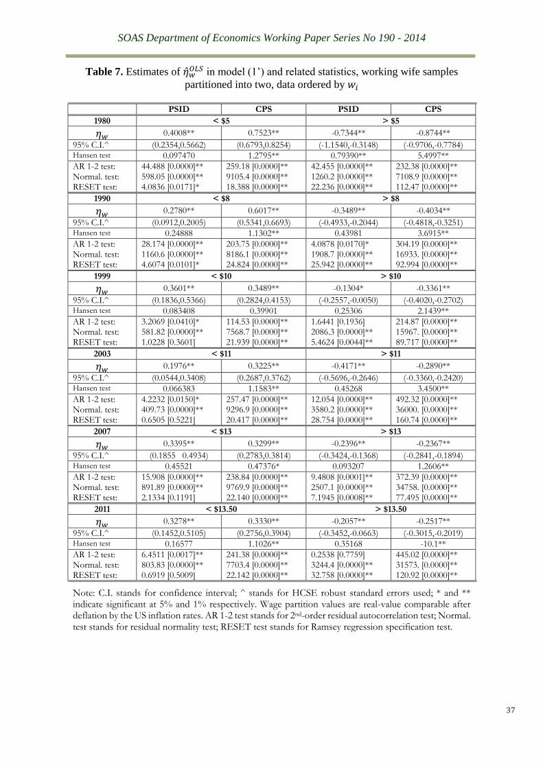
SOAS Department of Economics Working Paper Series No 190 - 2014
37
Table 7. Estimates of �̂�𝑤𝑂𝐿𝑆 in model (1’) and related statistics, working wife samples
partitioned into two, data ordered by 𝑤𝑖
PSID CPS PSID CPS
1980 < $5 > $5
𝜂𝑤 0.4008** 0.7523** -0.7344** -0.8744**
95% C.I.^ (0.2354,0.5662) (0.6793,0.8254) (-1.1540,-0.3148) (-0.9706,-0.7784) Hansen test 0.097470 1.2795** 0.79390** 5.4997**
AR 1-2 test: Normal. test: RESET test:
44.488 [0.0000]** 598.05 [0.0000]** 4.0836 [0.0171]*
259.18 [0.0000]** 9105.4 [0.0000]** 18.388 [0.0000]**
42.455 [0.0000]** 1260.2 [0.0000]** 22.236 [0.0000]**
232.38 [0.0000]** 7108.9 [0.0000]** 112.47 [0.0000]**
1990 < $8 > $8
𝜂𝑤 0.2780** 0.6017** -0.3489** -0.4034**
95% C.I.^ (0.0912,0.2005) (0.5341,0.6693) (-0.4933,-0.2044) (-0.4818,-0.3251) Hansen test 0.24888 1.1302** 0.43981 3.6915**
AR 1-2 test: Normal. test: RESET test:
28.174 [0.0000]** 1160.6 [0.0000]** 4.6074 [0.0101]*
203.75 [0.0000]** 8186.1 [0.0000]** 24.824 [0.0000]**
4.0878 [0.0170]* 1908.7 [0.0000]** 25.942 [0.0000]**
304.19 [0.0000]** 16933. [0.0000]** 92.994 [0.0000]**
1999 < $10 > $10
𝜂𝑤 0.3601** 0.3489** -0.1304* -0.3361**
95% C.I.^ (0.1836,0.5366) (0.2824,0.4153) (-0.2557,-0.0050) (-0.4020,-0.2702) Hansen test 0.083408 0.39901 0.25306 2.1439**
AR 1-2 test: Normal. test: RESET test:
3.2069 [0.0410]* 581.82 [0.0000]** 1.0228 [0.3601]
114.53 [0.0000]** 7568.7 [0.0000]** 21.939 [0.0000]**
1.6441 [0.1936] 2086.3 [0.0000]** 5.4624 [0.0044]**
214.87 [0.0000]** 15967. [0.0000]** 89.717 [0.0000]**
2003 < $11 > $11
𝜂𝑤 0.1976** 0.3225** -0.4171** -0.2890**
95% C.I.^ (0.0544,0.3408) (0.2687,0.3762) (-0.5696,-0.2646) (-0.3360,-0.2420) Hansen test 0.066383 1.1583** 0.45268 3.4500**
AR 1-2 test: Normal. test: RESET test:
4.2232 [0.0150]* 409.73 [0.0000]** 0.6505 [0.5221]
257.47 [0.0000]** 9296.9 [0.0000]** 20.417 [0.0000]**
12.054 [0.0000]** 3580.2 [0.0000]** 28.754 [0.0000]**
492.32 [0.0000]** 36000. [0.0000]** 160.74 [0.0000]**
2007 < $13 > $13
𝜂𝑤 0.3395** 0.3299** -0.2396** -0.2367**
95% C.I.^ (0.1855 0.4934) (0.2783,0.3814) (-0.3424,-0.1368) (-0.2841,-0.1894) Hansen test 0.45521 0.47376* 0.093207 1.2606**
AR 1-2 test: Normal. test: RESET test:
15.908 [0.0000]** 891.89 [0.0000]** 2.1334 [0.1191]
238.84 [0.0000]** 9769.9 [0.0000]** 22.140 [0.0000]**
9.4808 [0.0001]** 2507.1 [0.0000]** 7.1945 [0.0008]**
372.39 [0.0000]** 34758. [0.0000]** 77.495 [0.0000]**
2011 < $13.50 > $13.50
𝜂𝑤 0.3278** 0.3330** -0.2057** -0.2517**
95% C.I.^ (0.1452,0.5105) (0.2756,0.3904) (-0.3452,-0.0663) (-0.3015,-0.2019) Hansen test 0.16577 1.1026** 0.35168 -10.1**
AR 1-2 test: Normal. test: RESET test:
6.4511 [0.0017]** 803.83 [0.0000]** 0.6919 [0.5009]
241.38 [0.0000]** 7703.4 [0.0000]** 22.142 [0.0000]**
0.2538 [0.7759] 3244.4 [0.0000]** 32.758 [0.0000]**
445.02 [0.0000]** 31573. [0.0000]** 120.92 [0.0000]**
Note: C.I. stands for confidence interval; ^ stands for HCSE robust standard errors used; * and ** indicate significant at 5% and 1% respectively. Wage partition values are real-value comparable after deflation by the US inflation rates. AR 1-2 test stands for 2nd-order residual autocorrelation test; Normal. test stands for residual normality test; RESET test stands for Ramsey regression specification test.
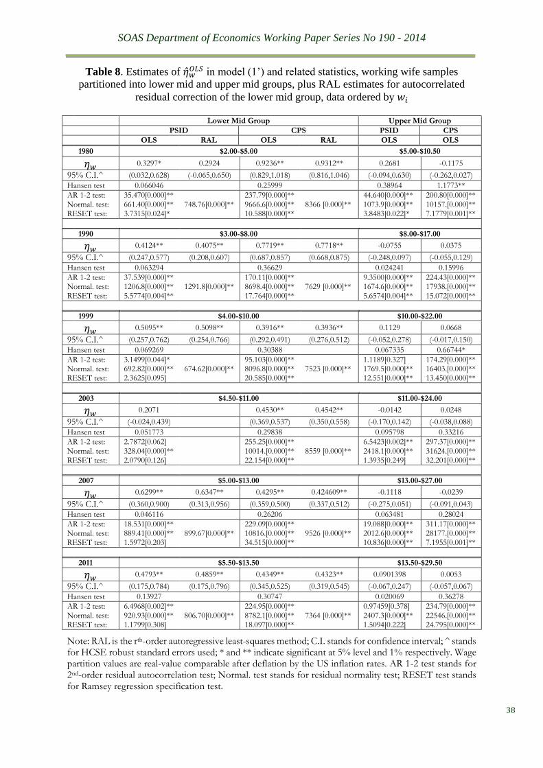
SOAS Department of Economics Working Paper Series No 190 - 2014
38
Table 8. Estimates of �̂�𝑤𝑂𝐿𝑆 in model (1’) and related statistics, working wife samples
partitioned into lower mid and upper mid groups, plus RAL estimates for autocorrelated
residual correction of the lower mid group, data ordered by 𝑤𝑖
Lower Mid Group Upper Mid Group
PSID CPS PSID CPS
OLS RAL OLS RAL OLS OLS
1980 $2.00-$5.00 $5.00-$10.50
𝜂𝑤 0.3297* 0.2924 0.9236** 0.9312** 0.2681 -0.1175
95% C.I.^ (0.032,0.628) (-0.065,0.650) (0.829,1.018) (0.816,1.046) (-0.094,0.630) (-0.262,0.027)
Hansen test 0.066046 0.25999 0.38964 1.1773**
AR 1-2 test: Normal. test: RESET test:
35.470[0.000]** 661.40[0.000]** 3.7315[0.024]*
748.76[0.000]**
237.79[0.000]** 9666.6[0.000]**10.588[0.000]**
8366 [0.000]**
44.640[0.000]** 1073.9[0.000]** 3.8483[0.022]*
200.80[0.000]** 10157.[0.000]** 7.1779[0.001]**
1990 $3.00-$8.00 $8.00-$17.00
𝜂𝑤 0.4124** 0.4075** 0.7719** 0.7718** -0.0755 0.0375
95% C.I.^ (0.247,0.577) (0.208,0.607) (0.687,0.857) (0.668,0.875) (-0.248,0.097) (-0.055,0.129)
Hansen test 0.063294 0.36629 0.024241 0.15996
AR 1-2 test: Normal. test: RESET test:
37.539[0.000]** 1206.8[0.000]** 5.5774[0.004]**
1291.8[0.000]**
170.11[0.000]** 8698.4[0.000]** 17.764[0.000]**
7629 [0.000]**
9.3500[0.000]** 1674.6[0.000]** 5.6574[0.004]**
224.43[0.000]** 17938.[0.000]** 15.072[0.000]**
1999 $4.00-$10.00 $10.00-$22.00
𝜂𝑤 0.5095** 0.5098** 0.3916** 0.3936** 0.1129 0.0668
95% C.I.^ (0.257,0.762) (0.254,0.766) (0.292,0.491) (0.276,0.512) (-0.052,0.278) (-0.017,0.150)
Hansen test 0.069269 0.30388 0.067335 0.66744*
AR 1-2 test: Normal. test: RESET test:
3.1499[0.044]* 692.82[0.000]** 2.3625[0.095]
674.62[0.000]**
95.103[0.000]** 8096.8[0.000]** 20.585[0.000]**
7523 [0.000]**
1.1189[0.327] 1769.5[0.000]** 12.551[0.000]**
174.29[0.000]** 16403.[0.000]** 13.450[0.000]**
2003 $4.50-$11.00 $11.00-$24.00
𝜂𝑤 0.2071 0.4530** 0.4542** -0.0142 0.0248
95% C.I.^ (-0.024,0.439) (0.369,0.537) (0.350,0.558) (-0.170,0.142) (-0.038,0.088)
Hansen test 0.051773 0.29838 0.095798 0.33216
AR 1-2 test: Normal. test: RESET test:
2.7872[0.062] 328.04[0.000]** 2.0790[0.126]
255.25[0.000]** 10014.[0.000]** 22.154[0.000]**
8559 [0.000]**
6.5423[0.002]** 2418.1[0.000]** 1.3935[0.249]
297.37[0.000]** 31624.[0.000]** 32.201[0.000]**
2007 $5.00-$13.00 $13.00-$27.00
𝜂𝑤 0.6299** 0.6347** 0.4295** 0.424609** -0.1118 -0.0239
95% C.I.^ (0.360,0.900) (0.313,0.956) (0.359,0.500) (0.337,0.512) (-0.275,0.051) (-0.091,0.043)
Hansen test 0.046116 0.26206 0.063481 0.28024
AR 1-2 test: Normal. test: RESET test:
18.531[0.000]** 889.41[0.000]** 1.5972[0.203]
899.67[0.000]**
229.09[0.000]** 10816.[0.000]** 34.515[0.000]**
9526 [0.000]**
19.088[0.000]** 2012.6[0.000]** 10.836[0.000]**
311.17[0.000]** 28177.[0.000]** 7.1955[0.001]**
2011 $5.50-$13.50 $13.50-$29.50
𝜂𝑤 0.4793** 0.4859** 0.4349** 0.4323** 0.0901398 0.0053
95% C.I.^ (0.175,0.784) (0.175,0.796) (0.345,0.525) (0.319,0.545) (-0.067,0.247) (-0.057,0.067)
Hansen test 0.13927 0.30747 0.020069 0.36278
AR 1-2 test: Normal. test: RESET test:
6.4968[0.002]** 920.93[0.000]** 1.1799[0.308]
806.70[0.000]**
224.95[0.000]** 8782.1[0.000]** 18.097[0.000]**
7364 [0.000]**
0.97459[0.378] 2407.3[0.000]** 1.5094[0.222]
234.79[0.000]** 22546.[0.000]** 24.795[0.000]**
Note: RAL is the rth-order autoregressive least-squares method; C.I. stands for confidence interval; ̂ stands for HCSE robust standard errors used; * and ** indicate significant at 5% level and 1% respectively. Wage partition values are real-value comparable after deflation by the US inflation rates. AR 1-2 test stands for 2nd-order residual autocorrelation test; Normal. test stands for residual normality test; RESET test stands for Ramsey regression specification test.
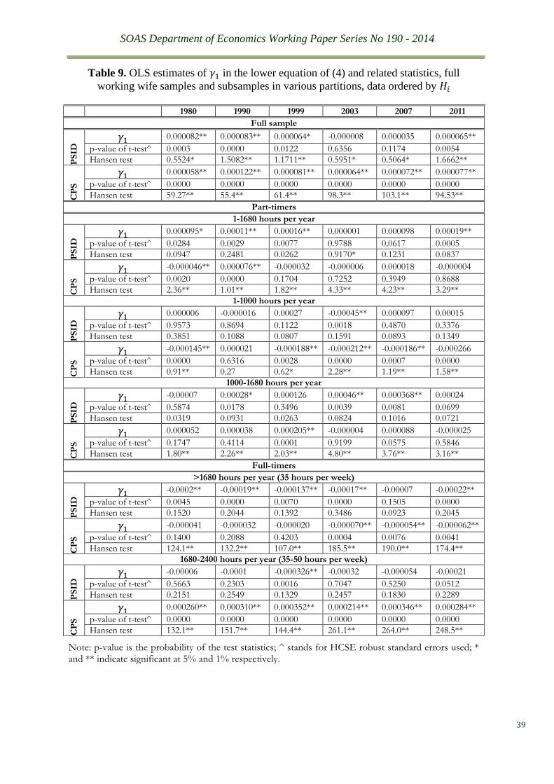
SOAS Department of Economics Working Paper Series No 190 - 2014
39
Table 9. OLS estimates of 𝛾1 in the lower equation of (4) and related statistics, full
working wife samples and subsamples in various partitions, data ordered by 𝐻𝑖
1980 1990 1999 2003 2007 2011
Full sample
PS
ID 𝛾1 0.000082** 0.000083** 0.000064* -0.000008 0.000035 0.000065**
p-value of t-test^ 0.0003 0.0000 0.0122 0.6356 0.1174 0.0054
Hansen test 0.5524* 1.5082** 1.1711** 0.5951* 0.5064* 1.6662**
CP
S
𝛾1 0.000058** 0.000122** 0.000081** 0.000064** 0.000072** 0.000077**
p-value of t-test^ 0.0000 0.0000 0.0000 0.0000 0.0000 0.0000
Hansen test 59.27** 55.4** 61.4** 98.3** 103.1** 94.53**
Part-timers
1-1680 hours per year
PS
ID 𝛾1 0.000095* 0.00011** 0.00016** 0.000001 0.000098 0.00019**
p-value of t-test^ 0.0284 0.0029 0.0077 0.9788 0.0617 0.0005
Hansen test 0.0947 0.2481 0.0262 0.9170* 0.1231 0.0837
CP
S
𝛾1 -0.000046** 0.000076** -0.000032 -0.000006 0.000018 -0.000004
p-value of t-test^ 0.0020 0.0000 0.1704 0.7252 0.3949 0.8688
Hansen test 2.36** 1.01** 1.82** 4.33** 4.23** 3.29**
1-1000 hours per year
PS
ID 𝛾1 0.000006 -0.000016 0.00027 -0.00045** 0.000097 0.00015
p-value of t-test^ 0.9573 0.8694 0.1122 0.0018 0.4870 0.3376
Hansen test 0.3851 0.1088 0.0807 0.1591 0.0893 0.1349
CP
S
𝛾1 -0.000145** 0.000021 -0.000188** -0.000212** -0.000186** -0.000266
p-value of t-test^ 0.0000 0.6316 0.0028 0.0000 0.0007 0.0000
Hansen test 0.91** 0.27 0.62* 2.28** 1.19** 1.58**
1000-1680 hours per year
PS
ID 𝛾1 -0.00007 0.00028* 0.000126 0.00046** 0.000368** 0.00024
p-value of t-test^ 0.5874 0.0178 0.3496 0.0039 0.0081 0.0699
Hansen test 0.0319 0.0931 0.0263 0.0824 0.1016 0.0721
CP
S
𝛾1 0.000052 0.000038 0.000205** -0.000004 0.000088 -0.000025
p-value of t-test^ 0.1747 0.4114 0.0001 0.9199 0.0575 0.5846
Hansen test 1.80** 2.26** 2.03** 4.80** 3.76** 3.16**
Full-timers
>1680 hours per year (35 hours per week)
PS
ID 𝛾1 -0.0002** -0.00019** -0.000137** -0.00017** -0.00007 -0.00022**
p-value of t-test^ 0.0045 0.0000 0.0070 0.0000 0.1505 0.0000
Hansen test 0.1520 0.2044 0.1392 0.3486 0.0923 0.2045
CP
S
𝛾1 -0.000041 -0.000032 -0.000020 -0.000070** -0.000054** -0.000062**
p-value of t-test^ 0.1400 0.2088 0.4203 0.0004 0.0076 0.0041
Hansen test 124.1** 132.2** 107.0** 185.5** 190.0** 174.4**
1680-2400 hours per year (35-50 hours per week)
PS
ID 𝛾1 -0.00006 -0.0001 -0.000326** -0.00032 -0.000054 -0.00021
p-value of t-test^ 0.5663 0.2303 0.0016 0.7047 0.5250 0.0512
Hansen test 0.2151 0.2549 0.1329 0.2457 0.1830 0.2289
CP
S
𝛾1 0.000260** 0.000310** 0.000352** 0.000214** 0.000346** 0.000284**
p-value of t-test^ 0.0000 0.0000 0.0000 0.0000 0.0000 0.0000
Hansen test 132.1** 151.7** 144.4** 261.1** 264.0** 248.5**
Note: p-value is the probability of the test statistics; ^ stands for HCSE robust standard errors used; * and ** indicate significant at 5% and 1% respectively.
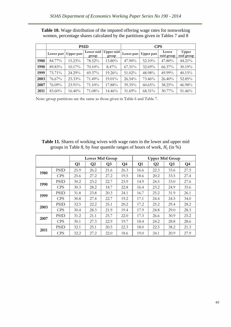
SOAS Department of Economics Working Paper Series No 190 - 2014
40
Table 10. Wage distribution of the imputed offering wage rates for nonworking
women, percentage shares calculated by the partitions given in Tables 7 and 8
PSID CPS
Lower part Upper part Lower mid
group Upper mid
group Lower part Upper part
Lower mid group
Upper mid group
1980 84.77% 15.23% 78.52% 13.80% 47.90% 52.10% 47.80% 44.21%
1990 89.83% 10.17% 70.10% 8.47% 67.31% 32.69% 66.37% 30.19%
1999 75.71% 24.29% 69.37% 19.26% 51.02% 48.98% 49.99% 40.15%
2003 76.67% 23.33% 71.49% 19.01% 26.54% 73.46% 26.40% 52.85%
2007 76.09% 23.91% 71.10% 17.88% 39.35% 60.65% 38.25% 46.98%
2011 83.60% 16.40% 71.08% 14.46% 31.69% 68.31% 30.77% 51.46%
Note: group partitions are the same as those given in Table 6 and Table 7.
Table 11. Shares of working wives with wage rates in the lower and upper mid
groups in Table 8, by four quantile ranges of hours of work, 𝐻𝑖 (in %)
Lower Mid Group Upper Mid Group
Q1 Q2 Q3 Q4 Q1 Q2 Q3 Q4
1980 PSID 25.9 26.2 21.6 26.3 16.6 22.3 33.6 27.5
CPS 25.6 27.2 27.2 19.5 18.6 20.2 33.5 27.4
1990 PSID 30.2 23.2 22.7 23.9 14.9 24.5 33.0 27.6
CPS 30.3 28.2 18.7 22.8 16.4 23.2 24.9 35.6
1999 PSID 31.8 23.8 20.3 24.1 16.7 25.2 31.9 26.1
CPS 30.8 27.4 22.7 19.2 17.1 24.4 24.5 34.0
2003 PSID 32.5 22.2 25.1 20.2 17.2 25.2 29.4 28.2
CPS 30.4 28.3 21.9 19.4 17.9 24.8 29.0 28.3
2007 PSID 31.2 21.1 25.7 22.0 17.3 26.6 30.9 25.2
CPS 30.1 27.3 22.9 19.7 18.4 24.2 28.8 28.6
2011 PSID 32.1 25.1 20.5 22.3 18.0 22.5 38.2 21.3
CPS 32.2 27.2 22.0 18.6 19.0 24.1 20.9 27.9
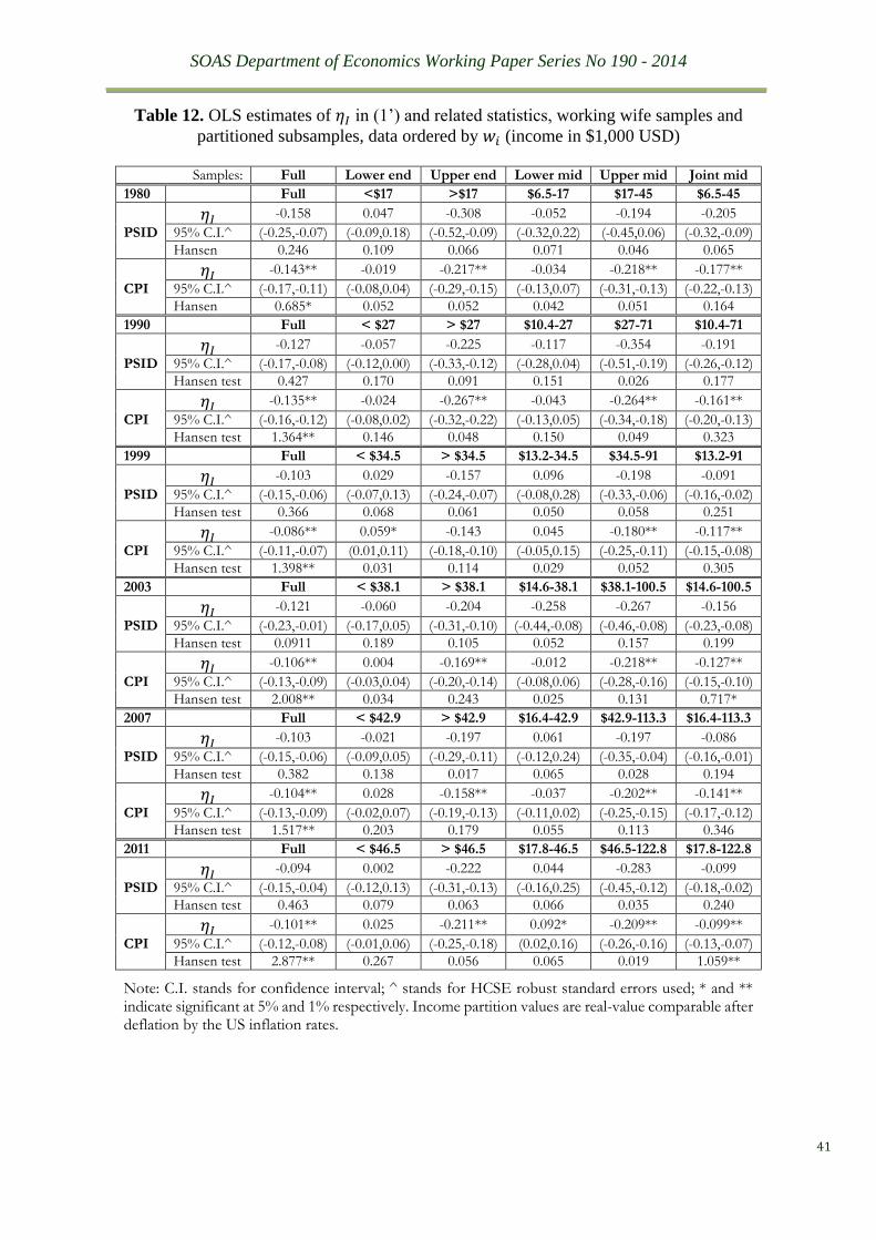
SOAS Department of Economics Working Paper Series No 190 - 2014
41
Table 12. OLS estimates of 𝜂𝐼 in (1’) and related statistics, working wife samples and
partitioned subsamples, data ordered by 𝑤𝑖 (income in $1,000 USD)
Samples: Full Lower end Upper end Lower mid Upper mid Joint mid
1980 Full <$17 >$17 $6.5-17 $17-45 $6.5-45
𝜂𝐼 -0.158 0.047 -0.308 -0.052 -0.194 -0.205
PSID 95% C.I.^ (-0.25,-0.07) (-0.09,0.18) (-0.52,-0.09) (-0.32,0.22) (-0.45,0.06) (-0.32,-0.09)
Hansen 0.246 0.109 0.066 0.071 0.046 0.065
𝜂𝐼 -0.143** -0.019 -0.217** -0.034 -0.218** -0.177**
CPI 95% C.I.^ (-0.17,-0.11) (-0.08,0.04) (-0.29,-0.15) (-0.13,0.07) (-0.31,-0.13) (-0.22,-0.13)
Hansen 0.685* 0.052 0.052 0.042 0.051 0.164
1990 Full < $27 > $27 $10.4-27 $27-71 $10.4-71
𝜂𝐼 -0.127 -0.057 -0.225 -0.117 -0.354 -0.191
PSID 95% C.I.^ (-0.17,-0.08) (-0.12,0.00) (-0.33,-0.12) (-0.28,0.04) (-0.51,-0.19) (-0.26,-0.12)
Hansen test 0.427 0.170 0.091 0.151 0.026 0.177
𝜂𝐼 -0.135** -0.024 -0.267** -0.043 -0.264** -0.161**
CPI 95% C.I.^ (-0.16,-0.12) (-0.08,0.02) (-0.32,-0.22) (-0.13,0.05) (-0.34,-0.18) (-0.20,-0.13)
Hansen test 1.364** 0.146 0.048 0.150 0.049 0.323
1999 Full < $34.5 > $34.5 $13.2-34.5 $34.5-91 $13.2-91
𝜂𝐼 -0.103 0.029 -0.157 0.096 -0.198 -0.091
PSID 95% C.I.^ (-0.15,-0.06) (-0.07,0.13) (-0.24,-0.07) (-0.08,0.28) (-0.33,-0.06) (-0.16,-0.02)
Hansen test 0.366 0.068 0.061 0.050 0.058 0.251
𝜂𝐼 -0.086** 0.059* -0.143 0.045 -0.180** -0.117**
CPI 95% C.I.^ (-0.11,-0.07) (0.01,0.11) (-0.18,-0.10) (-0.05,0.15) (-0.25,-0.11) (-0.15,-0.08)
Hansen test 1.398** 0.031 0.114 0.029 0.052 0.305
2003 Full < $38.1 > $38.1 $14.6-38.1 $38.1-100.5 $14.6-100.5
𝜂𝐼 -0.121 -0.060 -0.204 -0.258 -0.267 -0.156
PSID 95% C.I.^ (-0.23,-0.01) (-0.17,0.05) (-0.31,-0.10) (-0.44,-0.08) (-0.46,-0.08) (-0.23,-0.08)
Hansen test 0.0911 0.189 0.105 0.052 0.157 0.199
𝜂𝐼 -0.106** 0.004 -0.169** -0.012 -0.218** -0.127**
CPI 95% C.I.^ (-0.13,-0.09) (-0.03,0.04) (-0.20,-0.14) (-0.08,0.06) (-0.28,-0.16) (-0.15,-0.10)
Hansen test 2.008** 0.034 0.243 0.025 0.131 0.717*
2007 Full < $42.9 > $42.9 $16.4-42.9 $42.9-113.3 $16.4-113.3
𝜂𝐼 -0.103 -0.021 -0.197 0.061 -0.197 -0.086
PSID 95% C.I.^ (-0.15,-0.06) (-0.09,0.05) (-0.29,-0.11) (-0.12,0.24) (-0.35,-0.04) (-0.16,-0.01)
Hansen test 0.382 0.138 0.017 0.065 0.028 0.194
𝜂𝐼 -0.104** 0.028 -0.158** -0.037 -0.202** -0.141**
CPI 95% C.I.^ (-0.13,-0.09) (-0.02,0.07) (-0.19,-0.13) (-0.11,0.02) (-0.25,-0.15) (-0.17,-0.12)
Hansen test 1.517** 0.203 0.179 0.055 0.113 0.346
2011 Full < $46.5 > $46.5 $17.8-46.5 $46.5-122.8 $17.8-122.8
𝜂𝐼 -0.094 0.002 -0.222 0.044 -0.283 -0.099
PSID 95% C.I.^ (-0.15,-0.04) (-0.12,0.13) (-0.31,-0.13) (-0.16,0.25) (-0.45,-0.12) (-0.18,-0.02)
Hansen test 0.463 0.079 0.063 0.066 0.035 0.240
𝜂𝐼 -0.101** 0.025 -0.211** 0.092* -0.209** -0.099**
CPI 95% C.I.^ (-0.12,-0.08) (-0.01,0.06) (-0.25,-0.18) (0.02,0.16) (-0.26,-0.16) (-0.13,-0.07)
Hansen test 2.877** 0.267 0.056 0.065 0.019 1.059**
Note: C.I. stands for confidence interval; ^ stands for HCSE robust standard errors used; * and ** indicate significant at 5% and 1% respectively. Income partition values are real-value comparable after deflation by the US inflation rates.
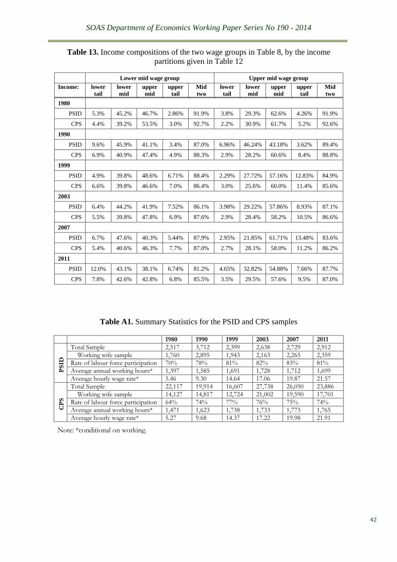
SOAS Department of Economics Working Paper Series No 190 - 2014
42
Table 13. Income compositions of the two wage groups in Table 8, by the income
partitions given in Table 12
Lower mid wage group Upper mid wage group
Income:
lower
tail
lower
mid
upper
mid
upper
tail
Mid
two
lower
tail
lower
mid
upper
mid
upper
tail
Mid
two
1980
PSID 5.3% 45.2% 46.7% 2.86% 91.9% 3.8% 29.3% 62.6% 4.26% 91.9%
CPS 4.4% 39.2% 53.5% 3.0% 92.7% 2.2% 30.9% 61.7% 5.2% 92.6%
1990
PSID 9.6% 45.9% 41.1% 3.4% 87.0% 6.96% 46.24% 43.18% 3.62% 89.4%
CPS 6.9% 40.9% 47.4% 4.9% 88.3% 2.9% 28.2% 60.6% 8.4% 88.8%
1999
PSID 4.9% 39.8% 48.6% 6.71% 88.4% 2.29% 27.72% 57.16% 12.83% 84.9%
CPS 6.6% 39.8% 46.6% 7.0% 86.4% 3.0% 25.6% 60.0% 11.4% 85.6%
2003
PSID 6.4% 44.2% 41.9% 7.52% 86.1% 3.98% 29.22% 57.86% 8.93% 87.1%
CPS 5.5% 39.8% 47.8% 6.9% 87.6% 2.9% 28.4% 58.2% 10.5% 86.6%
2007
PSID 6.7% 47.6% 40.3% 5.44% 87.9% 2.95% 21.85% 61.71% 13.48% 83.6%
CPS 5.4% 40.6% 46.3% 7.7% 87.0% 2.7% 28.1% 58.0% 11.2% 86.2%
2011
PSID 12.0% 43.1% 38.1% 6.74% 81.2% 4.65% 32.82% 54.88% 7.66% 87.7%
CPS 7.8% 42.6% 42.8% 6.8% 85.5% 3.5% 29.5% 57.6% 9.5% 87.0%
Table A1. Summary Statistics for the PSID and CPS samples
1980 1990 1999 2003 2007 2011
PS
ID
Total Sample 2,517 3,712 2,399 2,638 2,729 2,912
Working wife sample 1,760 2,895 1,943 2,163 2,265 2,359
Rate of labour force participation 70% 78% 81% 82% 83% 81%
Average annual working hours* 1,397 1,585 1,691 1,728 1,712 1,699
Average hourly wage rate* 5.46 9.30 14.64 17.06 19.87 21.57
CP
S
Total Sample 22,117 19,914 16,607 27,738 26,050 23,886
Working wife sample 14,127 14,817 12,724 21,002 19,590 17,701
Rate of labour force participation 64% 74% 77% 76% 75% 74%
Average annual working hours* 1,471 1,623 1,738 1,733 1,773 1,765
Average hourly wage rate* 5.27 9.68 14.37 17.22 19.98 21.91
Note: *conditional on working.
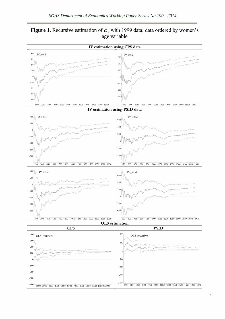
SOAS Department of Economics Working Paper Series No 190 - 2014
43
Figure 1. Recursive estimation of 𝛼1 with 1999 data; data ordered by women’s
age variable
IV estimation using CPS data
IV estimation using PSID data
OLS estimation
CPS PSID
1000 2000 3000 4000 5000 6000 7000 8000 9000 10000 11000 12000
-400
-300
-200
-100
0
100
200
300
400IV_set 1
1000 2000 3000 4000 5000 6000 7000 8000 9000 10000 11000 12000
-300
-200
-100
0
100
200
300
IV_set 3
150 300 450 600 750 900 1050 1200 1350 1500 1650 1800 1950
-800
-600
-400
-200
0
200
400 IV set 1
150 300 450 600 750 900 1050 1200 1350 1500 1650 1800 1950
-400
-200
0
200
400
600
IV_set 2
150 300 450 600 750 900 1050 1200 1350 1500 1650 1800 1950
-800
-600
-400
-200
0
200
400 IV_set 3
150 300 450 600 750 900 1050 1200 1350 1500 1650 1800 1950
-400
-200
0
200
400
600
IV_set 4
1000 2000 3000 4000 5000 6000 7000 8000 9000 10000 11000 12000-400
-300
-200
-100
0
100
200
300
400OLS_recursive
150 300 450 600 750 900 1050 1200 1350 1500 1650 1800 1950-1000
-750
-500
-250
0
250
500OLS_recursive
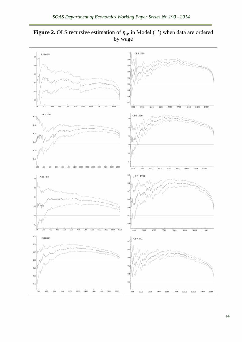
SOAS Department of Economics Working Paper Series No 190 - 2014
44
Figure 2. OLS recursive estimation of 𝜂𝑤 in Model (1’) when data are ordered
by wage
150 300 450 600 750 900 1050 1200 1350 1500 1650
0.0
0.2
0.4
0.6
0.8
1.0
PSID 1980
1000 2500 4000 5500 7000 8500 10000 11500 13000
-0.6
-0.4
-0.2
0.0
0.2
0.4
0.6
0.8
1.0 CPS 1980
200 400 600 800 1000 1200 1400 1600 1800 2000 2200 2400 2600 2800
-0.4
-0.2
0.0
0.2
0.4
0.6
PSID 1990
1000 2500 4000 5500 7000 8500 10000 11500 13000
-0.4
-0.2
0.0
0.2
0.4
0.6
CPS 1990
150 300 450 600 750 900 1050 1200 1350 1500 1650 1800 1950
-0.2
0.0
0.2
0.4
0.6
0.8PSID 1999
1000 2500 4000 5500 7000 8500 10000 11500
-0.1
0.0
0.1
0.2
0.3
0.4
0.5CPS 1999
200 400 600 800 1000 1200 1400 1600 1800 2000 2200
-0.75
-0.50
-0.25
0.00
0.25
0.50
0.75PSID 2007
1000 3000 5000 7000 9000 11000 13000 15000 17000 19000
0.0
0.1
0.2
0.3
0.4
0.5
CPS 2007
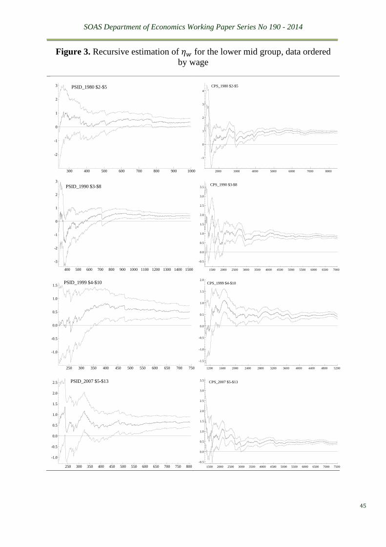
SOAS Department of Economics Working Paper Series No 190 - 2014
45
Figure 3. Recursive estimation of 𝜂𝑤 for the lower mid group, data ordered
by wage
300 400 500 600 700 800 900 1000
-2
-1
0
1
2
3 PSID_1980 $2-$5
2000 3000 4000 5000 6000 7000 8000
-1
0
1
2
3
4
CPS_1980 $2-$5
400 500 600 700 800 900 1000 1100 1200 1300 1400 1500
-3
-2
-1
0
1
2
3
PSID_1990 $3-$8
1500 2000 2500 3000 3500 4000 4500 5000 5500 6000 6500 7000
-0.5
0.0
0.5
1.0
1.5
2.0
2.5
3.0
3.5CPS_1990 $3-$8
250 300 350 400 450 500 550 600 650 700 750
-1.0
-0.5
0.0
0.5
1.0
1.5PSID_1999 $4-$10
1200 1600 2000 2400 2800 3200 3600 4000 4400 4800 5200
-1.5
-1.0
-0.5
0.0
0.5
1.0
1.5
2.0CPS_1999 $4-$10
250 300 350 400 450 500 550 600 650 700 750 800
-1.0
-0.5
0.0
0.5
1.0
1.5
2.0
2.5 PSID_2007 $5-$13
1500 2000 2500 3000 3500 4000 4500 5000 5500 6000 6500 7000 7500
-0.5
0.0
0.5
1.0
1.5
2.0
2.5
3.0
3.5CPS_2007 $5-$13
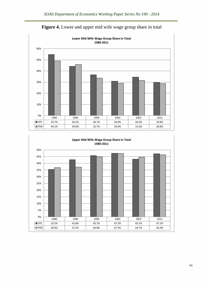
SOAS Department of Economics Working Paper Series No 190 - 2014
46
Figure 4. Lower and upper mid wife wage group share in total
1980 1990 1999 2003 2007 2011
CPS 54.7% 44.2% 36.7% 30.9% 34.5% 29.8%
PSID 49.1% 45.8% 33.7% 29.0% 31.6% 28.8%
0%
10%
20%
30%
40%
50%
60%
Lower Mid Wife Wage Group Share in Total1980-2011
1980 1990 1999 2003 2007 2011
CPS 35.5% 42.8% 45.7% 47.5% 43.1% 47.1%
PSID 36.9% 37.2% 44.8% 47.3% 44.7% 46.4%
0%
5%
10%
15%
20%
25%
30%
35%
40%
45%
50%
Upper Mid Wife Wage Group Share in Total1980-2011

SOAS Department of Economics Working Paper Series No 190 - 2014
47
Figure 5. Distribution of wife’s and husbands’ wage rates in 1980 and 2011
-1
-0.8
-0.6
-0.4
-0.2
0
0.2
0.4
0.6
0.8
1
0 0.5 1 1.5 2 2.5 3 3.5 4 4.5 5 5.5
-1500
-1000
-500
0
500
1000
1500
Log Hourly Wage Distribution for Wife and Husband CPS 1980 (left: frequency, right: normal density)
husband
wife
norm density
-1
-0.8
-0.6
-0.4
-0.2
0
0.2
0.4
0.6
0.8
1
-250
-150
-50
50
150
250
0.0 0.5 1.0 1.5 2.0 2.5 3.0 3.5 4.0 4.5 5.0
Log Hourly Wage Distribution for Wife and Husband PSID 1980 (left: frequency, right: normal density)
wife
husband
normal density
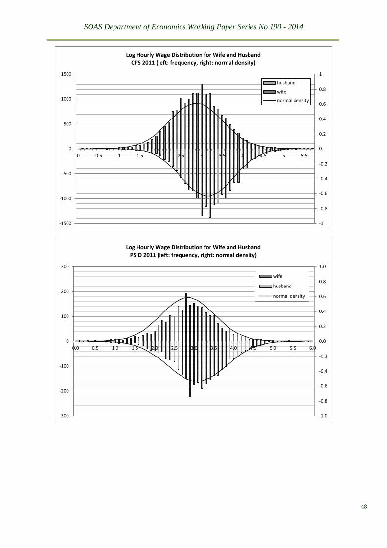
SOAS Department of Economics Working Paper Series No 190 - 2014
48
-1
-0.8
-0.6
-0.4
-0.2
0
0.2
0.4
0.6
0.8
1
-1500
-1000
-500
0
500
1000
1500
0 0.5 1 1.5 2 2.5 3 3.5 4 4.5 5 5.5
Log Hourly Wage Distribution for Wife and Husband CPS 2011 (left: frequency, right: normal density)
husband
wife
normal density
-1.0
-0.8
-0.6
-0.4
-0.2
0.0
0.2
0.4
0.6
0.8
1.0
-300
-200
-100
0
100
200
300
0.0 0.5 1.0 1.5 2.0 2.5 3.0 3.5 4.0 4.5 5.0 5.5 6.0
Log Hourly Wage Distribution for Wife and Husband PSID 2011 (left: frequency, right: normal density)
wife
husband
normal density