--R 1 3 2 1 3 U S E O F L AND S T D I G I T A L D A T A F O R S N O W C O

V E R APP IN G I 1 / 1

13 THE UPPER SAINT JON .(U) COLD REGIONS RESEARCH AND IENGINEERING LAB HANOVER NH C J MERRY ET AL. JUN 97

UNCL ASSIFIEL-:R7- F/S8,12 NL

smmhhhhmhhlmIII"."'mmmo

'UA

ak

w .- - ~ -w# w-' .fl -z

7L-)

REPO T 878 DO FIE ~p US rmy orp

Col Rein esac

Enieeig aortr

Yt..

For conversion of Si metric units to U.S.IBritishcustomary units of measurement consult ASTMStandard E380, Metric Practice Guide, publishedby the American Society for Testing and Materi-als, 1916 Race St., Philadelphia, Pa. 19103.

!0

*Cover Landsa t MSS Image (scene ID E-306 72-14443-5) acquired during the 1979-80season for the Upper St. John RiverBasin.

Jl 1o

.5.-; CL*

- ?9

J 4.

" ,:Covr:.I~adsa MS imae (cen ,D.-3'.2

CRREL Report 87-8June 1987

Use of Landsat digital data forsnow cover mapping in theUpper Saint John River Basin, Maine

Carolyn J. Merry and Michael S. MillerAccession For

UTIS GRA&IDTIC TAB lUnannounced 1]jut $f oatio------

Distribution/Availability Codes

Avail end/orDat/Spec alDist Soii

DTICSELCT ED

E

OFFICE OF THE CHIEF OF ENGINEERS

Approved for public retem; distribution is unlimited.

6a. NAME OF PERFORMING ORGANIZATION I6b. OFFICE SYMBOL 7a. NAME OF MONITORING ORGANIZATIONU.S. Army Cold Regions Research (If applicable)and Engineering Laboratory j CRREL Office of the Chief of Engineers

6C. ADDRESS (Cty, State, and ZIPCode) 7b. ADDRESS (City, State, and ZiP Code)

Hanover, New Hampshire 03755-1290 Washington, D.C. 20314-1000

$a. NAME OF FUNDING /SPONSORING Bb. OFFICE SYMBOL 9. PROCUREMENT INSTRUMENT IDENTIFICATION NUMBERORGANIZATION I f applicable)

8c. ADDRESS (Ciy, State, and ZIP Code) 10. SOURCE OF FUNDING NUMBERSPROGRAM PROJECT TASK WORK UNITELEMENT NO. NO. NO, ACCESSION NO

WIS 3158411. TITLE (nclude Security Classification)

Use of Landsat Digital Data for Snow Cover Mapping in the Upper Saint John River Basin, Maine

12. PERSONAL AUTHOR(S)Merry, Carolyn J. and Miller, Michael S.

13a._TYPE OF REPORT 13b. TIME COVERED 14. DATE OF REPORT (Year, Month, Day) 15. PAGE COUNTFROM TO juTlneIR I 7416. SUPPLEMENTARY NOTATION

17 / COSATI CODES '18. SUBJECT TERMS (Continue on reverse if necessary and identify by block number)/ FIELD GROUP SUB-GROUP Hydrologic modeling Runoff

Landsat Snow coverRemote sensing Snow water equivalent

19. ABSTRACT (Continue on reverse if necessary and identify by block number)Measurements of snow depth and its water equivalent were obtained at 11 snow courses in the Allagash,Maine, area in conjunction with Wi acquisition of five Landsat-2 and -3 images during the 1977-78 and1978-79 winters. To test a hypothesis that Landsat reflected radiance values on a regional scale do change,histograms of the Landsat MSS band 7 reflected radiance values for a 300-,'x,300-pixel (420Lki- area nearAllagash were evaluated to quantify the change. A statistical description (skewness and kurtosis) of thehistogram for each scene was developed and then correlated with ground measurements of snow depth.A snow index based on skewness and modal popul tion was found to correlate well with snow depth. Fol-lowing these initial results,4he Landsat data wergre-examined and corrections were made for solar eleva-tion and MSS sensor calibration. Thatreflected radiance from open areas showed a consistent increase inintensity with increasing snow depth. Vtriqorested land cover classes did not change with snow depth.Digital imagery data acquired (! 31 May 1978 when the land was snow-free was used to classify land covercategories. Ground truth measurements of water equivalent of the snow cover were area-weighted usingthe land cover classification to derive regional values on each of the five Landsat winter scenes. The

20 DISTRIBUTION/AVAILABILITY OF ABSTRACT 21 ABSTRACT SECURITY CLASSIFICATIONC1 UNCLASSIFIED/UNLIMITED 0 SAME AS RPT 0 DTIC USERS Unclassified

221. NAME OF RESPONSIBLE INDIVIDUAL 22b TELEPHONE (Include Area Code) 22c OFFICE SYMBOLMerry. Carolyn J. 603-646-4100 11RR .- RF.

Unelmdfied

19.bstract (cont'd)

'---- 1March 1978 snow measurement of 19.46 cm of water equivalent was used as an input value to theSSARR model. The SSARR prediction for the 1 March-31 May 1978 'imeperiod was within 78% ofthe measured runoff for the initial baseflow period and within 66% measured for the spring melt re-cession period. However, the timing of six observed runoff peaks was off by 2 to 9 days. The magni-tude of five of t e predicted runoff peaks was within 75% of the recorded streamflow. Additionalwork on calibrati g the basin peak timing and melt rate factors is required.

U i f

ii Unclassified

PREFACE

This report was prepared by Carolyn J. Merry, Research Physical Scientist, Geo-logical Sciences Branch, Research Division, U.S. Army Cold Regions Research andEngineering Laboratory, and Michael S. Miller, M/A-COM Sigma Data Inc., God-dard Institute for Space Studies.

The study was sponsored under the Corps of Engineers Civil Works Remote Sens-ing Research Program, CWIS 31584, Snow Cover Analysis Using Landsat DigitalData.

The authors express their appreciation to Dr. Harlan L. McKim for his supportand helpful technical discussions on the project; to Saul Cooper (formerly Chief,Water Control Branch, U.S. Army Engineer Division-New England) and Dr. JerryBrown for their support throughout the project; to Roy Bates (CRREL), to Mary-Lynn Brown (CRREL) and Lenora Wong (formerly with U.S. Air Force Academy)for assistance in reduction of the meteorological and snow course data; to JudyKaren (formerly with Dartmouth College) and Nancy H. Humiston (CRREL) forcomputer input of certain data files; to Roy Gardner for his invaluable assistance inmaking the snow courses in conjunction with the Landsat satellite overpasses; toRoy Bates and Harold O'Brien (CRREL) for their assistance in selecting the snowcourse sites and for technical review of this report; to Gary DeCoff (CRREL) andJeffrey W. Doyle (Dartmouth College) for their work in adapting the SSARR modelto run on a PRIME 400 computer; to Timothy Pangburn for his technical assistancewhen running the SSARR model; to Lawrence W. Gatto and Richard K. Haugen fortechnical review of earlier results from this project; and to Dr. Stephen G. Ungar(NASA GISS) and the GISS programming staff for development of the Landsatcomputer algorithms used in the analysis of the Landsat digital data.

The contents of this report are not to be used for advertising or promotional pur-poses. Citation of trade names does not constitute an official endorsement or ap-proval of the use of such commercial products.

iii

~ ~ ~~~~~~~~~~~M Ao A.. AM, .Y,. . .v '.,m 1

CONTENTSPage

Abtract..........................................................in

In tro d u ctio n .......................... ... IBackground .. . . . . . . . . . . . . . . . . . . . . . . . . . . . . . I

Literature review for remote sensing of snow cover.........................1ILandsat CCTs ................................................... 12The computer algorithm ............................................ 13Physical setting ................................................... 17The SSARR model................................................. 19

Approach......................................................... 20Results and discussion................................................ 23

Histogram analysis-uncorrected Landsat data ........................... 23Histogram analysis-corrected and resampled Landsat data .................. 30Landsat data as input to the SSARR model.............................. 50

Conclusions ....................................................... 52Literature cited ..................................................... 52Appendix A: Snow depth and water equivalent data ......................... 58Appendix B: Meteorological and hydrologic data for the Upper Saint John River

Basin........................................................... 63

ILLUSTRATIONS

Figure1. Typical spectral reflectance curve for snow ............................ 82. Albedo ranges for tundra and boreal forest regions ....................... 93. Typical albedos for selected conditions ranging from water to ice- and snow-

covered lakes............................................... 104. Landsat orbital tracks over the northern Maine area ...................... 135. The concept of the four-dimensional "color" space used in the computer clas-

sification algorithm .......................................... 166. Location of the outflow points for the Ninemile Bridge, Dickey, and Allagash

subbasins of the Upper Saint John River Basin...................... 187. Schematic of the SSARR model .................................... 198. Locations of the I I snow courses in the Allagash, Maine, area............... 219. Snow depth and water equivalent values durin the Landsat overpasses ........ 22

10. Landsat histograms for the total 300- x 300-pixel area located near Allagash,Maine .................................................... 24

11. Landsat histograms for the softwoods class ............................ 2512. Landsat histograms for the hardwoods class ........................... 2613. Landsat histograms for the mixed forest class .......................... 2714. Landsat histograms for the open area class ........................... 2815. Landsat histograms for the water class................................ 2916. Landsat histograms (corrected) for the total 300- x 300-pixel area located near

Allagash, Maine ............................................ 3117. Landsat histograms (corrected) for the softwoods class .................... 32

1v

Page

18. Landsat histograms (corrected) for the hardwoods class .................... 3319. Landuat histograms (corrected) for the mixed forest class ................... 3420. Landsat histograms (corrected) for the open areas class ..................... 3521. Landsat histograms (corrected) for the water class ......................... 3622. Landsat histograms (corrected and resampled) for the total 300- x 300-pixel

area located near Allagash, Maine .................................. 3823. Landsat histograms (corrected and resampled) for the softwoods class ........ 3924. Landsat histograms (corrected and resampled) for the hardwoods class ....... 4025. Landsat histograms (corrected and resampled) for the mixed forest class ...... 4126. Landsat histograms (corrected and resampled) for the open areas class ........ 4227. Landsat histograms (corrected and resampled) for the water class ............ 4328. SSARR model run for the I March to 31 May time period ................... 51

TALES

Table1. Parameters affecting albedo and emissivity of snow ........................ 122. Landsat satellite overpasses for the Upper Saint'John River Basin ............ 143. Snow course site characteristics in the Allagash area, Maine ................. 204. Landsat estimates of regional snow depth compared to available ground meas-

urements .. .... ...................................... 305. Satellite parameters used in the correction of Landsat data .................. 376. Statistics of MSS band 5 histograms ..................................... 447. Statistics of MSS band 7 histograms ..................................... 468. Average snow depth for each land cover class and total area ................. 489. Areal determination of snow depth and water equivalent for the basin ........ 50

v

I-

-iOa

Use of sat Digital Data for Snow Cover MappingIn the Upper Saint John River Basin, Maine

CAROLYN J. MERRY AND MICHAEL S. MILLER

INTRODUCTION Because of the remoteness of the area, it wouldbe very costly to establish a data collection net-

The U.S. Army Cold Regions Research and En- work for evaluating the water equivalent of thegineering Laboratory (CRREL). along with the snowpack each year. However, estimates of theU.S. Army Engineer Division, New England amount of water available in the snowpack are re-(NED), have been involved in the Landsat data quired for flood control during spring runoff.collection system and Landsat imagery analysis There were two objectives for this study. Thesince the launch of ERTS-I, now known as Land- first objective was to analyze the Lane . digitalsat-I, in July 1972 (Cooper et al. 1975). During the data to determine if there is a correlation betweenLandsat-l experiment, CRAEL participated in the snow depth and the measured intensities in thedata collection system studies by developing sen- ,ar spectral bands. The second objective was tosor interfaces for the Landsat data collection plat- determine how satellite multispectral data can beforms (DCPs) and evaluating the system perfor- used in the SSARR model. The areal distributionmance of various DCP installations. During the of mapped land cover categories was area-weight-Landsat-2 program (1975-77), CRREL was in- ed using snow course measurements that allowed avolved in the digital processing of the Landsat basinwide value of water equivalent to be calcu-computer-compatible tapes (CCTs) and in DCP lated for each land-cover category. This estimatesensor and software interface development. The of snow-cover water equivalent was input to thehydrologic parameters selected for Landsat digital SSARR model and compared to recorded streamanalysis were snow cover and delineation of wet- flow measurements.lands and flooded areas (Merry and McKim 1978).This report summarizes the continuation of theLandsat program, with funding from the Office of BACKGROUNDthe Chief of Engineers, from the winter of 1977-78 through the 1979-80 winter season. Literature review for

Each spring the SSARR (Streamflow Synthesis remote sensing of swow coverand Reservoir Regulation) model is used to fore- Barry (1983) conducted a survey of recent ad-cast snowmelt and precipitation runoff in the Up- vances in selected areas of snow and ice researchper Saint John River Basin in northern Maine. from 1979 to 1982. Results obtained by new meas-There are two ways to input snow to the SSARR urement techniques and the application of remotemodel: one is to input the percentage of the water- sensing methods were described.shed area covered by snow, and the second is to in- Manual methods have been used to delineate theput a basinwide average value of water equivalent. areal extent of snow and the mean altitude of theHowever, present methods of using point snow snowline from Landsat Multispectral Scannercourse measurements to calculate a basinwide Subsystem (MSS) photographic data productsmean snow-water equivalent value can provide er- (Meier 1973, 1975a; Barnes and Bowley 1974; Ras-roneous data because of nonrepresentative snow mussen and Ffolliott 1979, Bowley et al. 1981).courses and inappropriate extrapolation methods. The Landsat MSS imagery is available for a

185-km square area in four spectral regions (two resolution available with the VHRR permits posi-visible bands of 0.5-0.6 pm and 0.6-0.7 ;m, and tioning of the snow limit to within 10 km (McGin-two near-infrared bands of 0.7-0.8 pm and 0.8- nis 1975). Snow depth estimates have been found1.1 pm). Attempts were made to estimate the snow to correlate well with snow brightness for snowdepth from Landsat MSS visible band imagery. depth measurements less than 25 cm, althoughSnow depths of 2.5 cm or more can be mapped re- there is insufficient ground snow depth observa-liably: it was found that the brightness level in- tions to conclude that satellite brightness valuescreases with an increase of the snow thickness to are a reliable indicator of snow depth (McGinnis15 cm (Barnes and Bowley 1974). Beyond this 1975).snow depth, however, changes in brightness do McGinnis (1975) examined a single NOAA-2not normally occur. The snow line can be mapped VHRR visible wavelength image over the south-to an accuracy of 20 km. A set of techniques for east U.S. following a major snow storm. The sat-satellite snow mapping are covered in Barnes and ellite data was gridded into 32- x 32-pixel areas,Bowley (1974). corresponding to 1024 sq km on the ground. The

Three regions were isolated on the TIROS (Tele- greatest snow depth within each cell, as reportedvision Infrared Observation Satellite) ESSA (Envi- in the Department of Commerce climatologicalronmental Sciences Services Administration) and summaries, was paired with the highest brightnessSoviet Meteor-10 system satellite imagery. They value. A power curve was found to describe the re-included: 1) a snow depth of less than 2.5 cm, 2) suiting plot. Small increases in depth causedsnow depth from 2.5 to 10.2 cm, and 3) snow brightness increases much larger than comparabledepth greater than 10.2 cm (Kurilova 1975, Kuri- increases at higher depths. McGinnis (1975) foundlova et al. 1976). Snow depths greater than 10.2 that "once the snow accumulates to about 25 cm,cm were approximated only when climatic infor- most small plants are covered, only the largermation on snow depth and weather conditions was shrubs and plants (corn stalks to trees) remain visi-available. The Meteor-10 satellite data are some- ble and in most cases will remain uncovered exceptwhat limited because of the low spatial resolution in some mountainous areas where extremely heavy(1.25 kin) of the photographs used in Kurilova's snows occur."studies. Matson and Wiesnet (1981) developed a moni-

Percent snow-covered area maps of water ba- toring program for the routine global mapping ofsins in the southwestern U.S., the Sierra Nevada in snow cover using visible-channel imagery from theCalifornia, the Pacific Northwest, and the north- NOAA satellites. The interannual variability of re-eastern U.S. are prepared weekly by NOAA/ gional snow cover can be described.NESS (National Oceanic and Atmospheric Ad- Lillesand et al. (1982) evaluated digital GOESministration/National Environmental Satellite visible data for four snow-covered days in Minne-Service) starting on 1 November and ending when sota. Brightness values were compared against 13the snowpack is depleted (McGinnis et al. 1979). rural nonforested sites located near NationalSince the 1977-78 winter season, operational coy- Weather Service snow depth measurement sites.erage has been maintained for 30 basins, with the Linear and second-order regression fits for the in-data supplied within 30 hr of a satellite overpass. dividual days resulted in variable RI results. Simi-The satellite images used for the snow mapping lar analysis for forested sites was not reported.are from the VHRR (Very High Resolution Radi- They did find that subtraction of non-snowometer) sensor on the NOAA satellite and the brightness values for an October image from theVISSR (Visible and Infrared Spin-Scan Radiom- snow image brightness values might have value ineter) on GOES (Geostationary Operational En- digitally determining the presence of snow in for-vironmental Satellite). The VHRR provides daily ested regions.coverage over the U.S. in the visible wavelengths Imagery from the ESSA-9 camera system oper-(0.6-0.7 pm) and twice-daily coverage in the ther- ating in the visible wavelengths was used to inter-mal infrared wavelength (10.5-12.5 pm) band at a pret snow conditions in the Quebec-Labrador re-spatial resolution of 1 km for 256 energy levels. gion (Parry and Grey 1975). The imagery has aThe VISSR imagery is available approximately spatial resolution of approximately 5 km and a rel-every half hour over the United States at several ative brightness scale of 64 levels. It was foundresolutions in the visible and thermal infrared that terrain factors, in particular the vegetationregions. The best resolution is 0.8 km for the visi- type, had a significant effect on the reflection val-ble band and 8 km for the thermal band. The -kIm ues and, under similar snow conditions, physio-

2

AL

graphic regions of the same type exhibit compar- in the visible part of the spectrum, and just slightlyable brightness values, less in the near infrared. Such snow, therefore, ap-

A series of five-day composite minimum bright- pears light toned on both visible and near-infraredness (CMB) charts were used in the analysis. Re- imagery. The surface of melting snow is coveredflection values were measured on a scale of 0-10% by a thin film of water that absorbs most of the in-reflection when using a Densichron densitometer. frared radiation and therefore melting snow ap-A frequency-density analysis of the histograms of pears dark on the infrared imagery" (Goldingreflection values was used to see if regional snow 1974). However, ice is quite absorptive also. Oldconditions could be determined. "A distribution or refrozen snow would probably appear dark-with high values and a moderate right skew repre- toned in the near infrared region, too.sents a fresh snowfall over the greater part of the The Nimbus-7 satellite, launched on 24 Octoberarea, whereas a bimodal distribution indicates that 1978, carries a multifrequency, dual-polarized mi-the snowfall was restricted to particular parts of crowave imager called the Scanning Multichannelthe region. With the same range of values and a Microwave Radiometer (SMMR). The goal ofleft skew, the snow conditions can be interpreted Kunzi et al. (1982) was "to show that the threeas intermediate, which suggests settling, redistri- snow-cover parameters: extent, snow water equiv-bution, ageing and compaction. A strongly uni- alent, and onset of snow melt can be determinedmodal, left-skew distribution indicates that the using scanning multichannel microwave radiom-melt stage had been reached, and the subsequent eter (SMMR) data... . Snow extent is determinedshift of the modal class toward lower values re- for dry snow cover with depth z 5 cm, snow waterflects the progressive expansion of the snowfree equivalent can be determined on a regional basisareas" (Parry and Grey 1975). with - 2 g/cm2 rms accuracy, and the onset of

There was a general consistency in the relative snow melt is clearly visible by the detection of meltbrightness of individual vegetation zones (in the and refreeze cycles prior to snow runoff" (Kunzirange and the mean of each group) at all stages of et al. 1982). However, the main limitation of thethe snow cover with the exception of the final melt satellite passive microwave data is the coarse spa-period. The differences between the vegetation tial resolution, varying from 30 to 60 km depend-zones were particularly noticeable after periods of ing on the frequency range (18-37 GHz). Kunzi etextensive snowfall. al. (1982) distinguished three classes of snow with

The High Resolution Infrared Radiometer the SMMR data, including 1) no snow, 2) dry(HRIR) provides for 24-hr mapping of the Earth snow, and 3) snow undergoing melt and refreezeat an 8.5-km resolution. Nighttime infrared meas- cycles. Two algorithms were developed to deter-urements of the Earth's surface and cloud top mine snow depth and snow water equivalent to antemperatures are provided in the 3.6- to 4.2-pm accuracy of 6 cm for snow depth and 2 g/cml forwavelength range; during the daytime the HRIR snow water equivalent based on the climaticmeasures reflected shortwave radiation in the regimes of Finland, southern Russia, and Canada0.7-to 1.3-jAm range. The Image Dissector Camera (Kunzi et al. 1982).System (IDCS) provides television coverage in the "Microwave instruments, such as the SMMR,0.5- to 0.7-1n range at a 4.1-km resolution. Imag- are the only remote sensors providing subsurfaceery from these two sensor systems was acquired snow data. ....The SMMR is a very promising sen-over the Lake Winnipeg and the Sierra Nevada sor for the detection of the onset of snow melt.areas. It was found that "use of the near infrarce This information is of great interest in snow hy-data in combination with the visible imagery ap- drology and meteorology, it allows estimation ofpears to permit the detection of thawing snow" the time of runoff from a basin, and combined(Strong et al. 1971). An explanation for the near- with the snow water equivalent information, al-infrared brightness reversal was that "surface lows prediction of the total water runoff" (Kunzimelting of the lake or snowpack caused the sur- et al. 1982).face to absorb in the infrared while still reflecting Landsat MSS (Multispectral Scanner Subsys-in the visible" (Strong et al. 1971). tem) band 5 (0.6-0.7 ,m) has been the most useful

Melting snow could also be distinguished from for detecting and mapping mountain snow coversnow that had not reached melting temperatures (Barnes and Bowley 1973). Changes in snowlineby using the visible and near-infrared bands of the elevation on two different dates ranging from 60Landsat MSS (Golding 1974). "Under clear skies, to 1220 m were mapped from the satellite imagery.fresh or dry snow has a reflectivity of about 90% The snow observed in MSS band 7 (0.8-1.1 Im)

3

would normally be a high-elevation dry snow, A quantitative measure of the water equivalentwhereas the dry and lower-elevation wet snow sur- of the snowpack has not been obtained fromfaces are seen in the MSS band 5 imagery (Barnes Landsat photographic data products. Normallyand Bowley 1974). Landsat data has been used in a number of snow-

Barnes and Bowley (1974) discuss the problems melt runoff studies, principally to map the arealof using satellite data to map snow. One problem extent of snow for use in predicting snowmelt-is cloud cover obscuration for the visible and in- derived streamflow (Anderson et al. 1974; Meierfrared systems. Passive and active microwave sen- 1975c; Rango 1975, 1978, 1981; Rango et al. 1975;sor systems may be a means to overcome this. In- Thompson 1975; Rango and Itten 1976; Rangoterpretation of the satellite data is another prob- and Salomonson 1976; Shunying et al. 1980;lem and includes distinguishing between snow and Shafer et al. 1981; Dey et al. 1983). For example,clouds, identifying snow in densely forested areas Landsat satellite data have been used to monitorand in areas within mountain shadows, distin- the disappearance of the snow cover throughoutguishing between snow and highly reflective rock the melting period (Rango 1980a, b; Martinec andtypes, and mapping irregular, gatchy snowlines. Rango 1981; Rango and Martinec 1981; Martinec

Landsat digital data for an alpine basin in Swit- 1982). Martinec (1975) developed a simple rainfallzerland were classified, using a supervised paral- runoff model that incorporates the snowmelt run-lelepiped discriminant classifier, into three classes: off portion. The model takes into account the var-1) terrain totally covered by snow, 2) the transition iability of the degree-day factor, discharge reces-zone-a mixture of melting snow patches and sion coefficients, and the areal extent of snow.snowfree parts, and 3) snowfree terrain (Lichten- The depletion curves relating the areal extent ofegger et al. 1981). In high mountainous areas, cli- snow cover to elapsed time were modified to relatematic changes with elevation play an important snow coverage to accumulated temperature thaw-role in snowmelt. The alpine basin was separated ing degree-days. The total discharge volume frominto three elevation zones of 500 m intervals and a drainage basin during the snowmelt season wasthen digitized. The areal extent of snow cover was simulated by using these depletion curves of thecalculated in terms of percentage for each eleva- snow coverage (Rango and Martinec 1979; Rangotion zone and used as input to a runoff model. 1980a,b, 1983). Rango and Martinec (1982) sug-

In another test site, located in the Upper Rhine, gested that the depletion curves that normally re-Lichtenegger et al. (1981) used the elevation data late the areal extent of the snow cover to elapsedthat was registered to a Landsat image to generate time be modified to relate the snow coverage tofour additional channels that included an eleva- the accumulated thawing degree-days to forecasttion zone, exposure angle, slope angle, and a lam- runoff. It was then possible to estimate the totalbertian brightness or reflectance map. During the snow accumulation of the basin compared toclassification process, the shadowed area could be previous years by observing the course of thedetected and radiometric corrections with respect modified depletion curve during the first fewto the incident radiation angle could be carried weeks of the snowmelt season. The water equiva-out. It then becomes possible to extrapolate the lent of the snow at the beginning of snowmelt wassnow coverage within a climatologically similar re- estimated, and an appropriate modified depletiongion when clouds are encountered on Landsat im- curve was selected to use in the snowmelt runoffagery. model (Rango and Martinec 1982, Rango 1983).

A digital terrain model (DTM) was matched Precipitation and air temperature are other inputwith two Landsat MSS scenes for a 1500-kml data required in the model. (The effect of solar ra-catchment area in eastern Switzerland (Seidel et al. diation is automatically included in the degree-day1983). A snow signature was developed from a factor in Martinec's model.) When the first satel-scattergram of Landsat MSS band 5 versus 7 for lite images are available for analysis, the resultsmapping snow and snow-free areas. The DTM from the runoff model can be compared with thedata were used to map the snow-cover distribution initial modified snow cover depletion curves. Anin percent with respect to slope and aspect for a updated, modified depletion curve can be ,.given elevation zone. This provides a promising prepared that will more closely match the actualtool to extrapolate the snow cover from a cloud- mapped snow cover to be used in runoff forecast-free area to other parts of the subbasin that may ing. A more detailed description of the model canbe cloud-covered. be found in Martinec et al. (1983).

, . c . **** *

The Applications Systems Verification and Langham and Power would prefer to use areallyTransfer (ASVT) program for using operational averaged radiances at a resolution similar toapplications of satellite snow-cover observations NOAA satellites (1 km). However, a multispectralwas conducted over four sites in the western Unit- or pattern recognition analysis may be used to de-ed States from 1976 to 1978. Based upon the Col- tect areas that combine the signatures of forestorado ASVT operational forecasting experience, a and snow cover (Meier and Evans 1975).projected 6-10% relative improvement in fore- Single-band radiance thresholding of Landsatcasting occurred, with a benefit-to-cost ratio of MSS band 5 data was the principal technique used72:1, principally in the areas of hydroelectric ener- in determining snow coverage for three Columbiagy and irrigation (Castruccio et al. 1981). Opera- River subbasins (Wiegman et al. 1975). The tech-tional application of Landsat imagery was limited nique was supplemented by an editing proceduredue to lack of data that was cloud-free and received that involved reference to hand-generated eleva-in real time. The infrequency of Landsat coverage tion contours. A thematic map showing snow(every 18 days) magnified these problems. cover was documented by: 1) photography, 2) a

Digital processing techniques have been used to numerical pixel count representative of the totalmap the areal extent of snow. Meier and Evans area of snow in the scene and within the basin(1975) compared in a qualitative manner seven boundary, and 3) an array of single-digit numbersmethods for estimating snow cover from Landsat depicting tenths of snow cover for 2.5-km2 gridimagery for several basins in Oregon and Wash- cells within the basin.ington. The seven methods were grouped into The changes in the areal extent of snow coverthree categories: manual, interactive computer an- measured on Landsat imagery have been found toalysis, and digital pattern recognition techniques. correlate with changes in water equivalent record-The precision of the digital pattern recognition ed by a snow pillow (Anderson et al. 1974). As thetechnique on a pixel-by-pixel analysis was found water equivalent of snow increased, the areal ex-to be excellent, but at high cost and with slow to tent of snow observed for the Caribou-Pokeraverage speed. The analysis normally produces Creek watershed also increased. Another Landsatsupplemental data. The technique is good for rec- manual interpretation method used a coded snowognizing snow in trees or in shadow. The satellite cover classification scheme to account for vegeta-images can be used to determine the mean altitude tion cover, density, aspect, elevation, and slope toof the snow line or the percent of snow-covered map the extent of snow (Katibah 1975a, b). Se-area as a function of altitude (Meier 1975a). In ad- quential aerial photography, Landsat imagery,dition, the calculated areal extent of snow has and ground data on elevation, slope, aspect, andbeen found to be in good agreement with data on vegetation type were used to develop a subjectivesnow-covered areas from satellite images. Snow- image interpretation key for a study conducted incovered area from Landsat images is obtained by the Feather River Watershed in Northern Cali-radiance slicing (selecting the appropriate shade of fornia (Draeger and Lauer 1974; Katibah 1975a,gray to define the snow/no snow boundary), radi- b; Sharp and Thomas 1975). A rapid and relative-ance-gradient slicing, time-lapse comparison (for ly simple manual interpretation technique wasinstance, comparing portions of the same image in used to estimate acreages and extent of snow cover

* a snow-free and snow-covered condition, or suc- on satellite imagery by comparing no-snow Land-cessive snow-covered images), and by multispec- sat images with corresponding snow-coveredtral analysis (Meier and Evans 1975). The Landsat Landsat images.data offers additional advantages of high resolu- Dallam and Foster (1975) used a snow-freetion, accurate map projection, and multispectral Landsat scene to map the cover types and to servedata allowing use of pattern recognition tech- as a reference base. Snow-covered Landsat scenesniques (Meier 1974, 1975a). were then registered to the base image, so that any

Landsat data were found to be unsuitable for given point could be referenced to a cover type.mapping the snowline in rolling forested terrain Training sites were chosen visually to represent(Langham and Power 1977). Electronic density different snow cover classes. A supervised classifi-slicing techniques were performed on the satellite cation was used to produce a map of snow distri-image. The resolution resulted in too great a sam- bution versus cover type. Alfoldi (1976) also usedpling density in the transition regions since multi- these basic concepts in a digital classification of apie minima were observed in the histograms. snow-covered Landsat scene. An enhancement of

5S a

the Landsat scene and subsequent classification ing snowmelt through the soil profile to the near-was accomplished. A histogram analysis was used est channel.to make relative judgments about the snow cover. Anderson and Pagenhart (1957) did a multipleAlfoldi (1976) suggested a simple technique for regression analysis and found that elevation, solarmonitoring the presence of snow by developing a energy, and vegetation were important parameterslibrary of reference histograms with known snow influencing snow accumulation. An extensive re-characteristics and comparing an unknown histo- view of the effects of elevation, aspect, and forestgram to estimate a best match. Prerequisites in- canopy on snow was accomplished by Meimanclude identical areal coverage, cloud-free test and (1970). He concluded that differences resultingreference images, and no major changes in the from canopy influences tend to be smaller thanland use/vegetative cover of the area. Alfoldi those associated with elevation changes. On the(1976) indicated that total pixel brightness assumed other hand, Anderson (1969) concluded thata greater degree of importance for snow mapping storm characteristics explain the longest variationwhen compared to the techniques of level slicing in snow accumulation. Patch (1981) found thatand band ratioing for digital image analysis of forest cover type may have the widest applicationsnow. He also indicated that snow cover mapping in the utility of forest parameters in determiningshould be done on the basis of environmental fac- snow accumulation. He indicated that the foresttors affecting snowmelt rather than an arbitrary cover could be of primary importance, as it can bespatial grid. Ground visibility of snow through fo- and is altered by man, affecting spatial snowpackliage and elevation were two suggested param- patterns and ultimately water yield and regime.eters. A snow mapping experiment comparing the

Average snowpack characteristics, as well as the identification of six snow-cover types was accom-variability of these characteristics, were found to plished using three image processing systems-relate mainly to vegetation cover (FitzGibbon and LARSYS Version 3, STANSORT-2, and GeneralDunne 1979). In many small- to medium-size Electric IMAGE-100 (Itten 1975). In addition,drainage basins in lowland areas, average snow- other studies have focused on digital analyses ofpack characteristics are uniform and are a product Landsat data in defining various snow-cover typesof the regional climate (FitzGibbon and Dunne (Bartolucci et al. 1975, Dallam and Foster 1975,1979). They found that variation of snow-cover Luther et al. 1975, Alfoldi 1976). In these studies aproperties was due to small-scale terrain interac- quantitative estimate of water equivalent contenttions, which include local topography and vegeta- associated with snow-cover types was not made. Intion, and the processes of snow-cover formation. one case it was suggested that spectral variationsFitzGibbon and Dunne demonstrated that snow- within the snowpack area could not be reliably de-cover properties in a small, lowland subarctic termined because of detector saturation problemsdrainage basin may be characterized according to (Bartolucci et al. 1975).vegetation cover as it controls snow redistribution Saturation of the MSS detector proved a prob-through drifting. It is important that the extent lem for a study conducted over the Americanand nature of the snow cover during the snowmelt River Basin in California (McMillan and McGin-be known, since the extent of snow cover partially nis 1975). A multiple regression equation was de-determines the production of meltwater and re- veloped to predict the average snowpack densityserves of water held in the pack (FitzGibbon and using the variables of MSS 7 radiance values, solarDunne 1979). declination, sum of average daily air temperature

Thomsen and Striffler (1980) classified the frac- above freezing since snowfall (thawing degreetional snow-covered area of a Landsat pixel by de- days), and snow course elevation. The results weretecting changes (differences in radiance) between a not totally acceptable for immediate use in thesnowfree scene and snow-covered Landsat scenes. Sierra Nevada. The average snowpack density wasThe water equivalent of the snow cover was in- estimated from in situ albedo measurements ob-ferred from the classified Landsat image, taking tained with two pyrheliometers (0.3-4.0 ln) forpixel elevation, aspect, and the image acquisition given site and storm data (McMillan and Smithdate into consideration. A watershed information 1975).system was developed to include a snowmelt run- Another study used simulated infrared Landsatoff simulation that uses a spatial data format to color composites and snow course data to estimatedrive snowmelt and lateral flow models for rout- water equivalent related to the snowpack (Sharp

6

1975). Sampling units on the Landsat image were basin in Saskatchewan, Manitoba, and North Da-mapped to determine the areal extent of snow. An kota. They compared brightness values to groundestimation of a snow water equivalent index was measurements of snow depth. A good correlationcalculated using a linear regression equation relat- was found between the two variables. They cau-ing the imagery to ground truth data. tion, however, that the region is mostly flat, grass-

Several researchers have reported techniques for covered terrain. The relationship between depthestimating snow depth with aerial surveys. Stein- and brightness, they conclude, would not be evi-hoff and Barnes (1976) used aerial remote sensing dent for complex forested landscapes.to determine by photogrammetric means the snow Mellor (1965) stated that remote sensing of thedepth over a limited number of ground control snow cover may have useful applications since thetargets. First, they photogrammetrically deter- magnitude and wavelength of reflectance varymined the ground surface elevation from aerial with snow types. The albedo for a layer of newphotography before snowfall. Using photography snow can be quite high, approaching 91 %; as theafter a snow event, comparable ground elevations new snow grains coalesce and coarsen in texturewere determined. The difference between the two the albedo falls steadily towards levels of 60 toelevations would give an estimate of the snow 70% (Bergen 1975). In addition, the spectral re-depth. Multiple regression equations were devel- flectance declines from the combination of densi-oped for a given area relating snow depth to eleva- fication and increased particle size associated withtion, aspect, degree of slope, melt date, and vege- aging (O'Brien and Munis 1975).tation density at various times during the melt sea- The albedo of a snow surface varies dependingson. Ideally, once a regression equation was devel- on the state of the surface. Fresh, undisturbedoped for an area, the snow depth and water equiv- snow commonly reflects more than 70% of incom-alent could be predicted by measuring the melt ing solar radiation (Kondratyev 1969, Budykodate and environmental variables. However, a 1974). A typical curve of reflectance as a functionuniform prediction of snow depth for an entire of wavelength shows a uniform high value greaterwatershed from a single point measurement was than 0.8 at wavelengths between 0.35 and 0.90 Itmnot possible. (Fig. 1). A marked drop in reflectance occurs in

Blyth et al. (1974) discussed a similar technique the near-infrared wavelengths, to a value less thanusing terrestrial-based stereopairs for determining 0.1, between 1.4 and 1.6 pan. High reflectance wasdepth differences for pre- and post-snow dates. found in the visible portion with a sharp decreaseThey found the estimates of depth to be within in reflectance between 0.7 to 1.5 pan (O'Brien and10% of the actual for 3-hectare study sites. Munis 1975). This drop in near-infrared reflec-

Warskow et al. (1975) conducted aerial surveys tance has been useful in discriminating snow sur-over a western hydrologic basin. They made visual faces from clouds in satellite imagery (Barnes andestimates of snow depth, using the interactions of Smallwood 1975, Bartolucci et al. 1975).snow cover and the surrounding features of the Several aging processes decrease the reflectivitylandscape. It was estimated that dark rocks would of a snow surface. Drifting, compaction, melt/be obscured by snow depths of 0-15 cm; grass freeze cycles, and micro-structure are so interre-stems would no longer be visible when the depth lated as to make it difficult to assess the precisereached 15-20 cm; and half-shrubs were used as role of each in changing reflectivity (O'Brien andindices for the range 15-30 cm. Logs, fences, or Munis 1975). They also report that for a snowpackmarkers were required for estimating snow depths that had been naturally aged for about 40 hours, agreater than 30 cm. It was found that estimates ratio of about 0.8 spectral reflectance occurred forwere accurate within ± 5 cm, which was sufficient fresh to aged snow over the visible and near-infra-for their runoff volume forecasts. red portions of the spectrum. This was for a spe-

Nicholson (1975) collected a temporal series of cific case, so different natural aging conditionsair photos to document the areal extent of snow- could result in different findings (H.W. O'Brien,pack duration throughout the melt season in a pers. comm., 1984).subarctic area of eastern Canada. Contours of Using in situ measurements, McMillan andduration, derived from the photographs, were re- Smith (1975) found the square of albedo to be alated to maximum depth contours. good predictor of the average snowpack density.

Ferguson and Lapczak (1977a,b) examined a Bergen (1975) found that for snow grains greaterportion of a NOAA-4 image over the Souris River than 1.5 mm in diameter, albedo variations are

7

1.0 , I I I I I I I I

Specimen No. 730212

Source-detector 0 W

Snow Condition Cold, sbtsdg"Iur" cOnsistentY

0.8 Snow Density 0.31 &/cm-

0 Snow Hardness ,,.e W'z0S

0

o 0.6-

a

0.4

Z

0.2

0.00.6 0.8 1.0 1.2 1.4 1.6 1.8 2.0 2.2 2.4

Wavelength, psm

Figure I. Typical spectral reflectance curve for snow (after O'Brien and Munis 1975).

primarily associated with density rather than grain and the darkness of the nearly black bodies (i.e.,size. In contrast, Bohren and Beschte (1979) re- trees and buildings, etc.)" (Kung et ai. 1964).ported no statistically significant change in albedo Thus, the structure of the vegetation canopy great-following artificial compaction by a snowmobile. ly influences the overall reflectivity. In their air-

For shallow snow cover, the reflective proper- plane measurements of surface beam albedo overties of the underlying surfaces affect the surface Wisconsin, Kung et al. (1964) found agriculturalalbedo. Multiple reflections within the snow allow lands under deep snow cover displayed albedos inpenetration of solar radiation to shallow depths. the range of 50 to 70%. "When the ground snowGiddings and La Chapelle (1961) show the extinc- cover is rather shallow, i.e., the snow depth is lesstion coefficient of snow to be a function of depth. than 5 in.,.the value of surface albedo is apparent-With an underlying black surface, they showed al- ly related to the depth of snow and in turn proba-bedo to increase rapidly with increasing depth, bly to the area of patches covered by the snow,leveling off sharply as depth increased beyond 20 though further accumulation of snow does notcm. O'Neill and Gray (1973) showed virtual inde- seem obviously to increase the albedo" (Kung etpendence of albedo from snow depth beyond al. 1964). Forested areas with deep snow reflecteddepths of approximately 10 cm. Wiscombe and between 20 and 50%4 of the incoming solar radia-Warren (1980) indicated that the depth at which tion. Species composition of the forest accountedbackground influences occur depends on density for considerable variability, for example, aspenand/or grain size. and birch forests had albedos ranging from 38 to

These observations are based on measurements 50%; pine forests ranged from 19 to 37%; oak 32of surfaces composed of pure snow. It may be ex- to 42%; northern hardwood 19 to 36%; and swamppected that the introduction of vegetation cano- conifer 25 to 38%.pies would complicate the relationship of snow McFadden and Ragotzkie (1967) presentedcover and albedo. hemispheric albedo data for a variety of snow-

In natural landscapes, the reflectivity of an area covered regions observed with hemispheric solar-during the winter will be determined by the unique imeters in flights over the boreal region of centralproperties of the surface components. "The re- Canada. Snow-covered tundra areas with frozengional albedo values during the winter months are lakes had abedos in the range 70 to 92%, whiledependent mainly on two factors, snow albedo forested lands with frozen lakes were in the range

8

go.

70Ae.()SO

40

3020

10

0 L0 1 2 3 4 5

swam .,m

Lowmne4l Ftm PuV frome No tike

-I ILight Ngrow mw Noma VqWI

Figure 2. Albedo ranges for tundra and boreal forest regions (after McFaddenand Ragotzke 1967).

30 to 68% (Fig. 2). With lakes only partly frozen, that was developed by Bauer and Dutton (1962),snow-covered forests had albedos of 23 to 55%. It Dutton (1962), Kung et al. (1964), and McFaddenwas found that the presence of frozen lakes raises and Ragotzkie (1967).regional albedos by a factor of at least 2 above Leonard and Eachner (1968) conducted albedothat of forests without lakes. Additional albedo measurements over a red pine plantation in north-data for other regions are shown in Figure 3 for se- ern New York State. On the morning following alected conditions ranging from water to ice- and snowfall of approximately 300 mm (30 mm watersnow-covered lakes. The more snow and ice cover equivalent), an estimated 100 mm (10 mm water

on a lake, the higher the albedo. equivalent) had been retained by the forest can-

The mechanics of obtaining hemispheric and opy. At this time, mean albedo as measured by abeam albedo are different. "Beam albedo is calcu- tramway elevated solarimeter was about 18%. Aslated from the output of an upward-facing hemi- the day progressed, a progressive decline in albedosphere radiometer and a radiometer with a was observed. Increasing temperature caused the

downward-facing parabolic mirror that intercepts dropping of clumps of snow, as well as some meltenergy from a small area with a 4 * beam width dripping. Most of the forest canopy was snow-freeand focuses this energy on the radiometer. Hemi- by 1300 hr. Albedo fell to approximately 15% andspheric albedo, on the other hand, is determined stayed fairly constant throughout the day. The re-from the records from the same type of upward- flectivity and canopy conditions during the after-facing radiometer and down-facing solarimeter noon were similar to measurements obtained im-that has a full 21r steradian field of view. At an mediately after a rainstorm. Leonard and Eschneraltitude of 500 ft the beam albedo system will in- suggest a value of 20% be used for albedo ofstantaneously sample an area 35 ft in diameter, snow-covered coniferous forest, although thiswhile the hemisphere system samples over the en- may be conservatively high.tire solid angle" (McFadden and Ragotzkie 1967). Using paired silicon cells above hardwood for-The values from the two different systems can be ests, Federer (1971) measured albedo at threecompared using a calibration factor of northern sites in New York State and New Hamp-

shire. Without snow, the canopy albedo was

(beam albedo x 1.294) = hemispheric albedo found to be about 10%. With ground snow cover,

9

I"I-

Abf bindm

100

0o

so

70

6o

"no. (%) s0

4030-

100

80

,oeo % 50I

20 $30 4

0 1 2 3 4 5

&OWS type

Lake condio Frozn Partly froze No IS MS--

Light No

8now Coverwsnow Snow

Figure3. Typcal abedos or selcted odiostnigfo ae oien

1000

lO0

so

Abodo (%) 50

40

30

2 0

Lake condkilon Frozen Paty frozen No Isku J

8nmlcovr Sow o mLight No

0- W1W Sow T -ft$an Sow

iqgure 3. Typical albedos for selected conditions ranging from water to ice- andSnow-covered lakes (data from McFadden and RagotZkie 1967). . I

v ',' , r', +,r+'rr~ , i" 'r',1 ' ' , W VW10'

the albedo increased to values of 20% to 30% reflection angles, must be known to interpret indi-(Federer 1971). vidual satellite measurements. The function hasChoudhury (1982) used Kung's aircraft albedo been measured at the snow surface and at the top

measurements (1964) to develop a model for the of the atmosphere, but its dependence on wave-effective albedo of partially snow-covered areas. length, snow grain size, and surface roughness isAn equation for the fractional snow-covered area, unknown (Warren 1982). Warren recommendsdependent upon the snowpack thickness, was de- that angular detailed measurements of the bidirec-veloped using Kung's data. These data were then tional reflectance for various wavelengths, graincompared to NOAA-2 VHRR data of McGinnis et sizes, and surface conditions should be given aal. (1975) for the southeastern United States. The high priority for remote sensing applications.predictions of the effective albedo model were in "Dozier et al. (1981) have used a model of Wis-qualitative agreement with McGinnis's observa- combe and Warren (1980) to calculate snow albe-tions; for a given snow depth, the calculated dos integrated over channels I and 2 (0.5-0.7 Inbrightness value was somewhat higher than the and 0.7-1.0 pm, respectively) of the NOA , TIROS-observed mean value (Choudhury 1982). N satellite. The hope is to deduce grain size from a

Spectral reflectance decreases with increasing near-infrared channel, where depth and contami-Spectale rizeflectae andeeaes with) iNrag nants have no effect on albedo, and then use the

particle size (Dunkle and Bevans 1956). Natural deduced grain size together with the channel Iaging of the snow with normal settling and densifi- data to infer snow water equivalent depth belowcation and th, metamorphism of the snow cover some threshold value around 100 mn. Among theor refreezing of partially melted snow on the sur- difficulties in this approach are (1) the conversionface and within the snowpack also cause a de- of bidirectional reflectance to albedo, (2) the poor

crease in reflectance (Dirmhirn and Eaton 1975, location of channel 2 for this purpose (an idealO'Brien and Munis 1975). Hoarfrost formation channel would be located in the region 1.0-1.2on the surface could also raise the reflectance pm, where the sensitivity of albedo to grain size is(H.W. O'Brien, pers. comm., 1984). The albedo greatest), and (3) the fact that visible albedo re-measurement of the snow cover changes with the duction can be due to impurities as well as to thin-

measremet ofthesnowcove chngeswiththening of the snowpack. Dozier et al. (1M8) werevarying contribution of specular reflection from apparentlyebleotoadetecotherthtnnin of9the snowthe snow surface with solar angle (Dirmhirn and apparently able to detect the thinning of the snow-

pack at the end of the melting season on someEaton 1975). Canadian lakes" (Warren 1982).

The reflectance of fine-grained snow is not Other research indicates that the 1.25- to 1.35-greatly dependent on wavelength in the visible re- pm spectral region would be an even better choicegion, since surface reflectivity is high and single due to the sensitivity of albedo to grain size (H.W.backscattering from the first layer of grains is ap- O'Brien, pers. comm., 1984).parently not very selective with respect to wave- O'Brien and Koh (1981) observed the change inlength (Mellor 1965). However, as grain size in- spectral reflectance with a few narrow-band filterscreases, reflectance and surface reflectivity de- as a thick snow cover decayed. They documentedcrease. A relatively large proportion of the reflect- in a qualitative manner the transition of the spec-ed light is backscattered from beneath the surface tral reflectance of snow to the spectral reflectanceso that reflectance becomes inversely dependent of grass.on wavelength (Mellor 1965). The magnitude and Several investigators reported that snow accum-wavelength dependence of reflectance will vary ulation is unique for specific vegetative and land-

with snow type (Mellor 1965). The reflectance of scape units (Steppuhn and Dyck 1974, Adamssnow is determined by the illumination conditions, 1976, Steppuhn 1976, Adams and Barr 1979, Fitz-by the surface characteristics, and by the subsur- Gibbon and Dunne 1979, Mathers 1980, Adamsface backscattering (Mellor 1977). and Roulet 1981). As discussed earlier, when con-

Warren (1982) reviewed the optical properties sidering an open, undisturbed snowpack, snowof snow in the solar (0.3 < :s 5/ m) and thermal depths greater than about 13 cm will not displayinfrared (5 < X s 40 um) wavelength regions, greater reflectivity with increasing accumulation.which are important for determining the climatic However, when the snow is found intermixed withrole of snow and for affecting snowmel. He states a vegetation canopy, the interactions are morethat the bidirectional reflectance distribution complex. It could be hypothesized that as thefunction, which is unevenly distributed among the bright snow increases in depth, the darker extent

%

11

of the plant cover (both horizontal and vertical) The Lasdmat CCTsbecomes obscured. The reflectance might in- The Landsat satellites (Landsat-l through -4)crease, ideally, until the uppermost crown of the circle the earth in a 920-kin, near-polar orbit oncevegetation is completely overlain by about 13 to 25 every 103 minutes, each completing approximatelycm of snow (McGinnis et al. 1975). 14 orbits per day. The multispectral scanner

Snow cover in different roughness zones shows (MSS) on each satellite is a line-scanning devicesystematic differences in snow water equivalent, that uses an oscillating mirror to continuouslyaverage density, and depth (Granberg 1975). Aver- scan perpendicular to the spacecraft (USGS andage water equivalent was found to be largely inde- NASA 1979). Six lines are scanned simultaneouslypendent of roughness zone, except for boundary in each of four spectral bands for each mirrorzones (Granberg 1975). Surface roughness com- sweep, and radiation is sensed simultaneously byprised topographic and vegetation roughness. The an array of six detectors in each of four spectralheight-to-width ratio of topographic roughness is bands from 0.5 to 1.1 jan (USGS and NASAconsiderably less than unity, and vegetation 1979). During image data processing, a black androughness has a height-to-width ratio considerably white photographic data product can be producedgreater than unity. The effect of roughness chang- of an area approximately 185 km on a side for thees through winter has shown that snow accumula- following spectral regions: MSS band 4 (0.5-0.6tion results in a progressive reduction in surface pm), MSS band 5 (0.6-0.7 jan), MSS band 6 (0.7-roughness (Granberg 1972). Six roughness zones 0.8 lam) and MSS band 7 (0.8-1.1 jm). This infor-were selected in Granberg's study and included mation is also available in digital form on a CCT. !,closed woodland, open woodland, regenerating Landsat data products can be obtained from the

burn, recent burn, bog, and lake. EROS Data Center, Sioux Falls, South Dakota.Warren (1982) and NASA (1982) listed the snow The standard Landsat CCT was computer-proc-

parameters affecting the visible, near-infrared, essed to produce a geometrically corrected tapethermal infrared, and microwave wavelength re- with the pixels transformed to a UTM (Universalgions (Table 1). "To detect individual snow pa- Transverse Mercator) projection. This geometric-rameters unambiguously from satellite, one must ally corrected CCT comprises 2432 scan lines, withtherefore examine the snow at several wavelengths each scan line covering 3200 pixels. Each pixel rep-simultaneously. For remote sensing applications, resents an area on the ground having dimensionsangularly detailed measurements of the bidirec- of 61 x 76 m. Differing levels of radiant energy fortional reflectance for various wavelengths, grain each pixel within the scene are registered on a scalesizes, and surface conditions should be given high from 0 to 127 (minimum (black] to maximumpriority" (Warren 1982). [white]) for bands 4, 5, and 6 and 0 to 63 for band

7 (Thomas 1975).

Table 1. Parameters affecting albedo and emissivityof snow (after Warren 1982 sad NASA 192). , 0AA

Visible Thermalsolar infrared Microwave

Snow property alberto emssivity emissivitY'

Grain (or crystal) size Yes* Yes YesZenith (or nadir) angle Yes" Yes YesSnow depth Yest YesContaminants YesLiquid water content Yes Yes YesSurface roughness Yes YesDensity Yes

Temperature Yes yesStratification YesSoil state, moisture, Yes

roughness, vegetation

If snowpack is thin or impurities are present.t Shallow, up to a few centimeters.

12

R 4 smws the Landsat orbital tracks over cate test sites more accurately. The classificationnorthwru New England. The ideal path and rows algorithms used were part of the GISS-MAPIfor Lwdat coverage over the Upper Saint John (Multispectral Image Analysis Package) program.River Basin were path 13, rows 27 and 28. How- In this package, digital count values for the fourever, side lap does occur with the adjacent paths Landsat MSS bands are converted to radiancesof 12 and 14. Table 2 shows the available Landsat (measured in mW cm"1/sr) using calibration-coverage over the Upper Saint John River Basin derived gains and offsets. The MAPI algorithmfor the 1977-78, 1978-79, and 1979-80 winter developed for analysis of the digital data allowsseasons. for both components of the data-one of the four

wavelength bands and the associated radiance val-The e"upsr al10lt ue for each pixel-to be evaluated when classify-

The geometric correction of the digital data and ing the Landsat data in various categories. Colorthe computer classification algorithms used in the differences consider the direction of the pixel vec-analyses were developed at the NASA Goddard tors relative to the four-band axes. Brightness dif-Institute for Space Studies (GISS) (Ungar 1977). ferences are based on the summation of the fourThe geometric correction provides for a 1:24,000 bands.scale computer print-out, which enables one to lo-

14 13 12 II

z

S----M.O

II5

I Mass 0 s0km

Figure 4. Landsat orbital tracks over the northern Mainearma. Image centers are indicated by the solid circles; the dashedoutin show pound coverag per franme and image overla and

13

Table 2. Lamdut satellite overpmes for the Upper Saint John River Basin.

a. I97-78 whew u . b. 198- wb mma

NASA Cloud NASA ClodDaR scw ID Path/row M*) Dome scen ID Path/row Mt)

I Dec 77 6044-14125 12/27 90 5 Dec 78 30275-14433 12/27 901 Dec 77 6044-14132 12/28 90 5 Dec 78 30275-14440 12/28 803 Dec 77 6046-14243 14/27 80 6 Dec 78 30276-14491 13/27 40

6 Dec 78 30276-14494 13/28 7019 Dec 77 6062-14122' 12/27 70 7Dec78 3027-14 1/28 0

19 Dec 77 6062-141250 12/28 90

20 Dec 77 6063-141800 13/27 20 23 Dec 78 30293-14432 12/27 8020 Dec 77 6063-141830 13/28 80 23 Dec 78 30293-14435 12/28 8021 Dec 77 6064-142350 14/27 80 24 Dec 78 30294-14491* 13/27 1021 Dec 77 6064-142410 14/28 90 24 Dec 78 30294-144930 13/28 0

6 Jan 78 2180-141210 12/27 10 25 Dec 78 30295-14552 14/28 90

6 Jan 78 21080-14124* 12/28 10 10 Jan 79 30311-14433 12/27 107 Jan 78 21081-1412* 13/28 60 10 Jan 79 30311-14435 12/28 108 Jan 78 21082-142340 14/27 80 II Jan 79 30312-14491* 13/27 108 Jan 78 21082-142410 14/28 90 11 Jan 79 30312-144940 13/28 0

24 Jan 77 21098-14123 12/27 80 12Jan70 30313-14552 14/28 10

24 Jan 77 21098-14130 12/28 60 19 Jan 79 21458-14295 12/27 025 Jan 77 21099-14182 13/27 90 19 Jan 79 21458-14301 12/28 025 Jan 77 21099-14184 13/28 90 28 Jan 79 30329-14433 12/27 9026 Jan 77 21100-14243 14/28 90 28 Jan 79 30329-14435 12/28 90

11 Feb 77 21116-141330 12/27 10 29 Jan 79 30330-14491 13/27 9011 Feb 77 21116-14140 12/28 20 29 Jan 79 30330--14494 13/28 9012 Feb 77 21117-141920 13/27 70 15 Feb 79 30347-14432 12/27 1012 Feb 77 21117-141950 13/28 70 15 Feb 79 30347-14435 12/28 013 Feb 77 21117-14251' 14/27 30 16Feb79 30348-14491 13/27 8013 Feb 77 21118-142530 14/28 30 16 Feb 79 30348-14493 13/28 60

I Mar 78 21134-141440 12/27 30 17 Feb 79 30349-14551 14/28 10I Mar 78 21134-141500 12/28 0 17 Feb 79 30349-14545* 14/292 Mar 78 21135-142030 13/27 30 5 Mar 79 30365-14431 12/27 902 Mar 78 21135-142050 13/28 10 5 Mar 79 30365-14434 12/28 903 Mar 78 21136-14264 14/28 50 6 Mar 79 30366-14485 13/27 90

9 Mar 78 30004-14421 12/27 10 7 Mar 79 30367-14550 14/28 909 Mar 78 30004-14423 12/28 10 23 Mar 79 30383-14430 12/27 30

28 Mar 78 30023-14414 12/27 90 23 Mar 79 30383-14432 12/28 1028 Mar 78 30023-14420 12/2 90 29 Apr 79 30420-14485 13/27 9029 Mar 78 30024-14472 13/27 80 29 Apr 79 30420-14492 13/28 9029 Mar 78 30024-14475 13/28 8030 Mar 78 30025-14533 14/28 90

15 Apr 78 30041-14415 12/27 9015 Apr 78 30041-14422 12/28 8017 Apr 78 30043-14534 14/28 70

25 Apr 78 21189-142350 13/28 9026 Apr 78 21190-142940 14/28 10

'Landsat CCTs available at CRREL.

14LL--

Tabie 2 (eut'd). The distance (length) of an observation from theorigin is a measure of the total radiance associated

e. 197960 w m mw with that point. The algorithm is primarily de-signed to combine observations that are similar in

NASA Clowd color into the same classification category. ThereJA . ID Plathrow MV) is provision for evaluating brightness differences

I Dec 79 30636-14454 13/27 9between pixels and for weighting these differences

I Dec 79 30636-14460 13/28 7 0 in with the color discriminant when constructing2 Dec 79 30637-14514 14/28 90 the classification categories.

18 Dec 79 30653-14393 12/27 0Discrimination based solely on color is obtained18 Dec 79 30653-14395 12/28 10 when the difference in direction between the solar19 Dec 79 30654-14451* 13/27 10 vectors (observations) is examined. If the angle be-19 Dec 79 30654-14453" 13/28 10 tween the observations is smaller than some user-20 Dec 79 30635-14512 14/28 10 defined criterion, the vectors are considered to be5 Jan 80 30671-143S5 12/27 10 lying in the same direction and, therefore, the ob-5 Jan 80 30671-14391 12/28 50 servations are placed in the same category.6 Jan 80 30672-14443 13/27 0 In addition to discrimination based solely on6 Jan 0 30672-14450 13/28 10 color, the GISS algorithm provides the capability

23 Jan 30 3063-14385 12/27 90 of weighting total radiance differences into the23an 0 30689-14392 12/28 90 discriminant equation for classification. The per-24Jan 0 30690-14444 13/27 3024 Jan 30 30690-14450 13/28 70 cent difference in brightness between two observa-

10 Feb 80 30707-14383 12/27 10 tions is computed. The calculated normalized dif-10 Feb 80 30707-14390 12/28 10 ference is then combined with the color difference11 Feb30 30708-14441 13/27 0 angle (expressed in steradians) by performing aIi Feb 30 30703-14444 13/28 40 weighted average in the RMS (root mean square)12 Feb 30 30709-14502 14/28 90 sense. This brightness-weighted quantity is now29 Feb 30 30726-14434 13/27 40 compared with the user-defined criterion (6.j.29 Feb 30 3026-144 13/28 90 Thus, in the classification process, a relatively17 Mar 30 30743-14372 12/27 70 small weighting of brightness allows very large17 Mar 80 30743-14374 12/28 70 brightness differences to disqualify observations18 Mar 30 30744-14430 13/27 90 that are similar in color from membership in theIS Mar 0 30744--14433 13/28 90 same category, thereby adding a second level of19 Mar 0 30745-14491 14/28 20discrimination.

4 Apr 30 30761-14364 12/27 70 There are two modes in which this classification4 Apr 30 30761-14370 12/28 905 Apr 30 30762-14422 13/27 90 scheme may be used: supervised and unsuper-5 Apr 30 30762-14424 13/28 90 vised. In the supervised mode the user specifies a

23 Apr 30 3073014414 13/27 90 signature, here shown as h, the energy distribution23 Apr 9D 370-14420 13/28 90 in the four Landsat bands. If an observation lies24 Apr 80 30781-14475 14/28 90 within a solid angle smaller than the user-defined

Landat CCTs available at CRREL. criterion, 6., it is said to belong to the categoryrepresented by the multispectral signature, B (Fig.5b). Therefore, all vectors * lying within a cone of

The Landsat MSS observation (pixel) may be angle b.. about signature B, which represents cat-thought of as a point in a four-dimensional "col- egory X, belong to category X.or" space, where the values along each axis repre- In the unsupervised classification a maximumsent the radiant energy received by the satellite in value of 6., is specified by the user for the com-one of the four bands (Fig. 5a). Observations that bined color-brightness difference. If the color-lie in a similar direction from the origin in this brightness difference is less than or equal to ,four-dimensional color space are said to be similar then pixels i and j are grouped into the same cate-in color regardless of their total radiant energy. gory.

IS7I

mm-

COLOR SAN,: ~D 3oTO/ I

I a-f SUPERVISED

I -/,, CLASSIFICATIONmm CAIUOSRYX

a, - mi il minaI/Lus aISAND I

- k a, M OAL A36NAMMSAND2

a. A color vector illustrated for three- b. Supervised mode. The user-defmed criter-dimensional space, but all four Landsat ion, 6m, defines category X about the signa-bands are used in the classification proc- ture B. Any color vector that lies within thisess. con belongs to category X. This is illustrated

for three bands, however, all four Landsatbands are used in the computer chwarfcationalgorithm.

-, / ArCTSOUN$WPENME .

OIASSIPICATBOAN 2 '

BMais 66MAX

c. Unsupervised mode. B, is similar in lirection to B2(60 s 6,.) and is placed in category 1. B is similar indirection to Bi and is placed in category 2. However, B,is also similar in direction to B, (category l. so categoryI is merged with category 2.

Figure 5. The concept of the four-dimensional "color" space used in the computer classification algorithm(after Merry et al. 1977).

To illustrate this in terms of equations used in The unit vector is used to def'me the direction ofthe computer analysis, each pixel's signature is the pixel. The magnitude of S is defined as therepresented by a real vector in the four-dimension- square root of the sum of the squares of the foural space. The signature is the sum of the four corn- components:ponents and is defined as the real vector represent-ed by the following equation: 1S[ i +/S? +1 + S ."+S (2)

= (S,,S,,S,,S,). (1) The unit vector is then defined as:

16

(3) 1977). In effect the unsupervised classification willS F - form several categories based on a criterion speci-

fying maximum color difference permissible bet-Note that the magnitude of unit vector S will ween members of the same category:always equal 1. The unit vector and real vector are

calculated for each pixel. Ab s 6 or W s 6 (7)Each pixel i and j is compared with every other

pixel in terms of color difference and brightness As shown, A is similar in direction to A, (cone ofdifference. The color difference is the absolute angle 6 s 6 and is placed in category I (Fig.value of the difference in the unit vectors: 3). A is similar in direction to A and is placed in

category 2. A is also similar in direction to vector= I- . (4) A (category 1). Therefore, category 1 is merged

with category 2.The brightness difference is the sum of the total When the pixels are chained together in clusters,radiance or brightness divided by two. This num- a cluster represents a category defimed by two ex-ber is divided into the absolute value of the differ- treme signatures. This hypothesis is due to the factence in the total radiances between two pixels: that pixels within certain ground cover classes dis-

play a continuous variation in signature over space

6 (Bi-Bj (5) between the two extreme signatures, for example,(Bi + B./2 ( mixtures of vegetation and urban areas. The com-

puter program searches for the pixel in a categoryThe differences in color and brightness between for which the color-brightness difference is larg-

pixels i and j are then combined to calculate an est, say i, and this pixel is called the first pureoverall signature difference between the two pix- type. Next the program determines the second pix-els. W is a parameter for specifying the relative el in that category that is furthest in terms of sig-weighting given to the color and brightness differ- nature from the first pure-type pixel. This pixel isences. The overall signature difference is defined then the second pure type, say Si .as: Once these two pure-type pixels are found, then

each pixel in that category can be expressed as alinear combination of the two pure types. There-

A&ij =/W6 + (1- W)66 (6) fore, the vector signature for an observed piel, S,is defined by the following equation, with Si and

If one suspects that the ground categories display 9i representing the two pure types (a two-compo-greater brightness differences than color differ- nent mixture) with 17 to define the fraction betweenences, one may wish to increase the importance of the two extremes:brightness differences when using the W param-eter to better differentiate among the ground cate- = + (I-1)Sj. (8)gories. If Wequals 0, then only the brightness dif-ference is used. If W is set to 1, then the color dif- The digital processing of the Landsat CCTs wasference is used for the signature difference be- accomplished through a cooperative agreementtween two pixels. with NASA GISS. Computer algorithms for the

In the unsupervised mode the color vector cor- analysis of the digital data were developed at GISSresponding to the first observation is compared to (Ungar 1977). These algorithms were accessed us-all subsequent observations. If color vector 1 is ing the CRREL remote entry terminal to the mainsimilar in direction to color vector 2 (i.e. 6 ! computer facility (IBM 4341), located at GISS in6,.), observation 2 is placed in the same category New York City.as the first observation (Fig. 5c). In a similar fash-ion, observations subsequent to observation 2 are Physical settingcompared to the second observation and so on, The Upper Saint John River Basin was selectedright up to the last observation. If in the process of because the SSARR model is used for operationalconstructing categories a member is found that flood forecasting by the New Brunswick Floodbelongs to a previous category, the new category is Forecast Centre. The subbasins evaluated includ-chained (or linked) to the original classification ed the Allagash (3240 km-), Dickey (7410 kin2),category, forming one joint category (Ungar and Ninemile Bridge (3340 km') (Fig. 6).

17

47*00

Theclmao0 iglgy S vtation oe

~46*00

70*00 69,00 W

Figure 6. Location of the outflow Points for the Ninemile Bridge (1), Dickey (2) and

Allagash (3) subbasins of the Upper Saint John River Basin.

The climate of this region is humid continental. The geology and vegetation of the area were

The average annual precipitation is approximately previously mapped and served as a data base of91 cm and occurs uniformly throughout the year, site characteristics in this study (McKim 1975,with about 30% in the form of snow. Average McKim and Merry 1975, Environmental Researchsnow depth ranges between 51 and 102 cm, with and Technology, Inc. 1977). Elevations within thethe upper limit exceeding 127 cm (New England subbasin range from 150 to 600 m, and forestDivision, Corps of Engineers 1967). Water equiva- cover varies from 76 to 930./lent of the snowpack reaches a maximum in late The snowpack in the Saint John River Basin isMarch and usually exceeds 25 cm. of shallow to medium depths of less than 30 cm of

18U

- 03i

water equivalent for an overall accumulation Flood Forecast Centre, Canada, to forecast run-(Hansen 1975). There are rare maximum accumu- off due to snowmelt and precipitation (Power etlations of 32 cm of water equivalent. The snow- al. 1980).pack melts and contributes to runoff in a time The SSARR model is a continuous deterministicperiod of less than 5 weeks. Coincident rainfall at simulation model of the river basin system (Fig.the time of snowmelt normally occurs during the 7). Streamflow is synthesized by evaluating snow-spring runoff. Ice movement also complicates the melt and rainfall. There are three basic compo-runoff process. nents in the SSARR model:

Most (85%) of the watershed is covered by a 1) A generalized watershed model for synthe-dense forest with predominantly coniferous for- sizing runoff from snowmelt, rainfall, or aests in the valleys and lower slopes. Hardwood combination of the two.forests cover the hilltops of minor relief. Mixed 2) A river system model for routing stream-forests occur principally along the valley sides. flows from upstream to downstream pointsForestry operations create new areas of clearcuts. through channel and lake storage.The region of study lies in the physiographic prov- 3) A reservoir regulation model in which reser-ince of the Chaleur Upland. The mean elevation voir outflow and contents may be analyzedof the upland province is 250 to 300 m. along with synthesized inflow and free flow

or any of several modes of operation (U.S.The SSARR model Army Engineer Division, North Pacific

The SSARR model was developed for use in the 1975).North Pacific Division of the U.S. Army Corps of In this study only the generalized watershedEngineers (U.S. Army Engineer Division, North portion of SSARR was used to predict outflowPacific 1975). The model is used for operational from the three gauging stations (Fig. 6).river forecasting and river management activities Snowmelt is calculated in the SSARR model byin connection with the Cooperative Columbia use of the temperature index method or a general-River Forecasting Unit, sponsored by the National ized snowmelt equation with additional options ofWeather Service, U.S. Army Corps of Engineers, subroutines for a snow-cover depletion approachand the Bonneville Power Administration. The or the elevation band approach. Because meteoro-SSARR model was previously calibrated for the logical data were available from a station near theSaint John River Basin by the New Brunswick Allagash gauging station, the temperature index

IUB aURFFALL

,1MOISTURE EVAPOTRANSPIRATION

I I S I

lrMOAMSTLOW

Figure 7. Schematic of the SSARR (Streamfiow Synthesis and Reser-voir Regulation) model (after U.S. Army Engineer Division, North

Pcfc17)

BS 1 IRC

FLWRNF

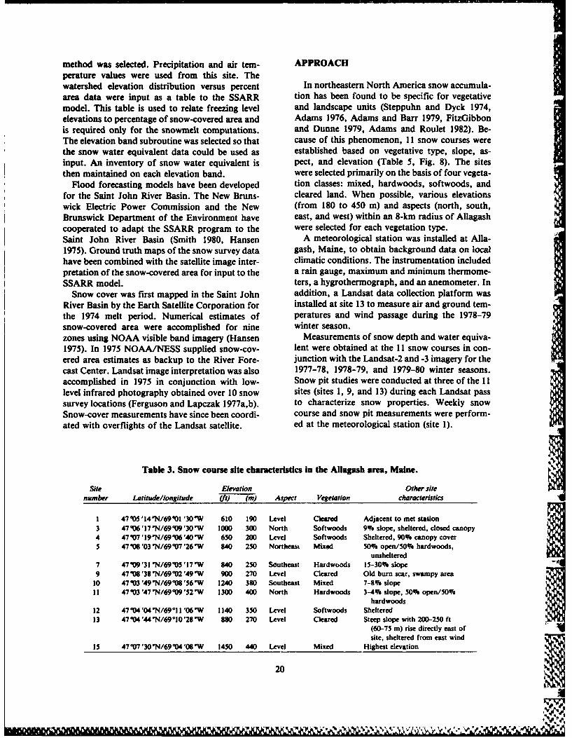
method was selected. Precipitation and air tern- APPROACHperature values were used from this site. Thewatershed elevation distribution versus percent In northeastern North America snow accumula-area data were input as a table to the SSARR tion has been found to be specific for vegetativemodel. This table is used to relate freezing level and landscape units (Steppuhn and Dyck 1974,elevations to percentage of snow-covered area and Adams 1976, Adams and Barr 1979, FitzGibbonis required only for the snowmelt computations. and Dunne 1979, Adams and Roulet 1982). Be-The elevation band subroutine was selected so that cause of this phenomenon, 11 snow courses werethe snow water equivalent data could be used as established based on vegetative type, slope, as-input. An inventory of snow water equivalent is pect, and elevation (Table 5, Fig. 8). The sitesthen maintained on each elevation band. were selected primarily on the basis of four vegeta-

Flood forecasting models have been developed tion classes: mixed, hardwoods, softwoods, andfor the Saint John River Basin. The New Bruns- cleared land. When possible, various elevationswick Electric Power Commission and the New (from 180 to 450 m) and aspects (north, south,Brunswick Department of the Environment have east, and west) within an 8-km radius of Allagashcooperated to adapt the SSARR program to the were selected for each vegetation type.Saint John River Basin (Smith 1980, Hansen A meteorological station was installed at Alla-1975). Ground truth maps of the snow survey data gash, Maine, to obtain background data on localhave been combined with the satellite image inter- climatic conditions. The instrumentation includedpretation of the snow-covered area for input to the a rain gauge, maximum and minimum thermome-SSARR model. ters, a hygrothermograph, and an anemometer. In

Snow cover was first mapped in the Saint John addition, a Landsat data collection platform wasRiver Basin by the Earth Satellite Corporation for installed at site 13 to measure air and ground tem-the 1974 melt period. Numerical estimates of peratures and wind passage during the 1978-79snow-covered area were accomplished for nine winter season.zones using NOAA visible band imagery (Hansen Measurements of snow depth and water equiva-1975). In 1975 NOAA/NESS supplied snow-coy- lent were obtained at the 11 snow courses in con-ered area estimates as backup to the River Fore- junction with the Landsat-2 and -3 imagery for thecast Center. Landsat image interpretation was also 1977-78, 1978-79, and 1979-80 winter seasons.accomplished in 1975 in conjunction with low- Snow pit studies were conducted at three of the 11level infrared photography obtained over 10 snow sites (sites 1, 9, and 13) during each Landsat passsurvey locations (Ferguson and Lapczak 1977a,b). to characterize snow properties. Weekly snowSnow-cover measurements have since been coordi- course and snow pit measurements were perform-ated with overflights of the Landsat satellite. ed at the meteorological station (site 1).

Table 3. Snow course site characteristics in the Allagash area, Maine.

Site Elevation Other sitenumber Latitude/longitude (ft) (m) Aspect Vegetation characteristics

1 47005 '14'N/69001 '30W 610 190 Level Cleared Adjacent to met station3 47006 '17 'N/69009'0"W 1000 300 North Softwoods 9% slope, sheltered, closed canopy4 47007 '19N/6906'40"W 650 200 Level Softwoods Sheltered, 90% canopy cover5 4708'03"N/69*07'26W 840 250 Northeast Mixed 50% open/50% hardwoods,

unsheltered7 47409'31 N/69005'17"W 840 250 Southeast Hardwoods 15-30% slope9 47008'38'N/69a02'49W 900 270 Level Cleared Old burn scar, swampy area

10 47003 '49 N/69a08 '56'W 1240 380 Southeast Mixed 7-8% slopeIi 47003 '47 N/69009'52 W 1300 400 North Hardwoods 3-4% slope, 50% open/50%

hardwoods12 47104'04"N/69°11 '06'W 1140 350 Level Softwoods Sheltered13 47'4'44N/69°10'28*W 880 270 Level Cleared Steep slope with 200-250 ft

(60-75 m) rise directly east ofsite, sheltered from east wind

Is 47007'30"N/69004'08 W 1450 440 Level Mixed Highest elevation

20I

lea., ?

47'10 Aireoon

ro I MI,

47*O0', mine area.

6 110 90'6'0

Figure 8. Locations of the 11 snow courses in theAllagash, Maine. area.

Figure 9 shows the maximum, minimum, and Maine, were investigated. The data for the fiveaverage values for snow depth and water equiva- winter scenes were registered with the assistance oflent for the I I snow course sites at the time of the a Ramtek image display unit. The I I snow courseLandsat satellite overpasses. Detailed tables on the sites were identified within the 300- x 300-pixelsnow depth and water equivalent data for each area. Individual band count values, band ratios,snow course site are shown in Appendix A. Ap- and band summations were evaluated. A solar ele-pendix B is a computerized listing of the daily me- vation correction was also applied to account forteorological data that was obtained during 1977- differences in insolation for the different Landsat80 at the Allagash site in support of the snow dates.cover mapping project. Additional meteorological A scene from 31 May 1978 was used to classifyinformation can be found in Bates (1983). the three subbasins using the GISS-MAPI algo-

The Landsat MSS digital data were analyzed to rithm. During this season the forest types coulddetermine whether a correlation existed between easily be separated due to the phenological state ofsnow depth and the measured intensities in the the deciduous trees. The young leaves of thesefour spectral bands. The five snow-covered Land- trees showed a high near-infrared reflectancesat scenes used in the analysis were the only ones (MSS 7) in comparison with that of the evergreenavailable that were relatively cloud-free: 6 January forest. The land cover types classified included1978, 11 February 1978, 1 March 1978, 24 Decem- water, open areas, softwoods, hardwoods, andber 1978, and I I January 1979. Histograms of the mixed forest. The selection of training sites forbrightness values in MSS band 7 for a 300- x classification of vegetation types was aided by the300-pixel (420 km2) area located near Allagash, use of aerial photography.

21

! I - -

120-

00

L0go -o

c Go0

LaC

S40-

j20-

20 7?on 25 It 2 20 7 25Dec- Ja- Feb. Mar Apr1977 1978

a. 1977-78 winter season.

120 11

E1~00

3800o

0

Z20-

6 15L 240 11 20 29 7 16 25 6 15 24 2 II 2

Dec '78 Jan'79 Feb Mar Apw

b. 1978-79 winter season.

FIgre 9. Snow depth and water equivalent values during the Landsat overpasses.

22

-' ~ , ~.~*-- V '~ % -r P.*p'741

120 I I

2100-

BO-U!

C

S40- f

a "20 3 9 24 110 29 IS 5,

Figure 9 (cont 'd).

servation date to another. Much of the skewnessUu tm amlue-.ImFkd observed in the regional histograms appears to re-

Lams data suit from the water and open area pixels. This isThe statistical analysis of the uncorrected Land- particularly noticeable for water surfaces because

sat data indicated that a direct correlation did not the absorption characteristic of water is replacedexist between snow depth and the measured inten- by an open expanse of highly reflective ice andsities in the four MSS spectral bands. This was snow cover.true in the comparison among the various snow For the forest cover classes, the shift in histo-course sites for a single Landsat scene and among gram shape is less dramatic. For the softwoodsthe various Landsat scenes for individual snow class there is little noticeable change in the shapecourse sites. or dimensions of the histogram between the Land-

Although the Landsat reflected-radiance values sat winter scenes and the 27 Oct 77 scene. Albedomeasured for a single pixel (0.45 hectare) did not investigations have shown that the more completeincrease (or decrease) uniformly with increasing closure of the softwood canopy precludes signifi-snow depth, it was hypothesized that on a regional cant reflectivity changes with a snowpackscale (> 26 km) changes in overall brightness (Leonard and Eschner 1968). The histograms formight occur. To test this hypothesis, histograms the hardwoods and mixed forest show a decreaseof the MSS 5 and 7 data were examined for the in kurtosis and a change of the histogram mode tofive winter scenes, the 31 May 78 scene, and an au- the brighter count values as the snow depth in-tumn scene from 27 October 1977. creases.

The MSS bands 5 and 7 count histograms for The MSS band 7 data were used to avoid thethe five land-cover classes and the total area for saturation of the MSS sensor that occurred in theeach of the six Landsat scenes are shown in Fig- other multispectral bands under snow conditions.ures 10. The count values for MSS 5 range from 0 In addition, the use of MSS 7 avoided the effectsto 127 and for MSS 7 range from 0 to 63. Although resulting from the decompression of MSS bands 4,the number of pixels varies from class to class due 5, and 6 that is applied during ground image proc-to the nature of the study site, the number of pix- essing of the Landsat data. The vegetation and

23

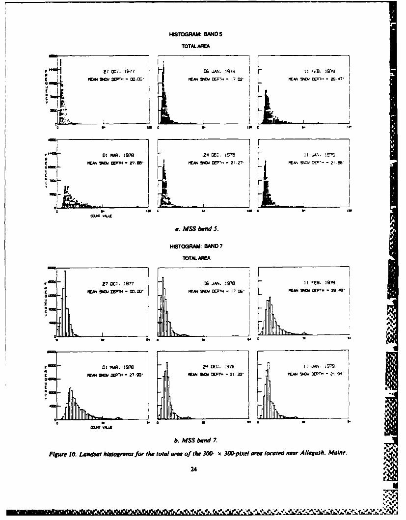
HISTOGRAM: BAND S

TOTAL AMA

ii 127OCT 1977 U0 JAN. 1578 11 FEB. 197!of L W M"PTH - M . MAN SNOWD.E:P-. - :7 Q2' PEAN 9"EPTH - 29.7-

e ,4 Ia n 0 54

9 WT - 27-.* W% '- , 2! .27 MEAN 90. MP- - 2: 95"

C 54 lU 0 54 0il 54 U

a. MS$ band S.

HISTOGRAM: BAND 7

TOTAL AREA

qm27 flCT. I2977 05 JAN. 1978 11 FEB. 1978

M W 9MI4TH - 00 MTEN OEPTH- 17'06- SNO CEPT -29.419

u

CI'

m I n*I. 2978 24 UEC. 1978 11 JAN

W-( 9" 00 V. -90'"nEA SWU D E rH - 21-33* PN 9 OE PTH -21 94-

0

C

0 3 5 0 3 40 a

b. MSS bend 7.

Rgw 10. Landsat hAiograms for the total area of the 300- x 300-pixel area located near Allagash, Maine.

24Ig.

C IL-U X ".0

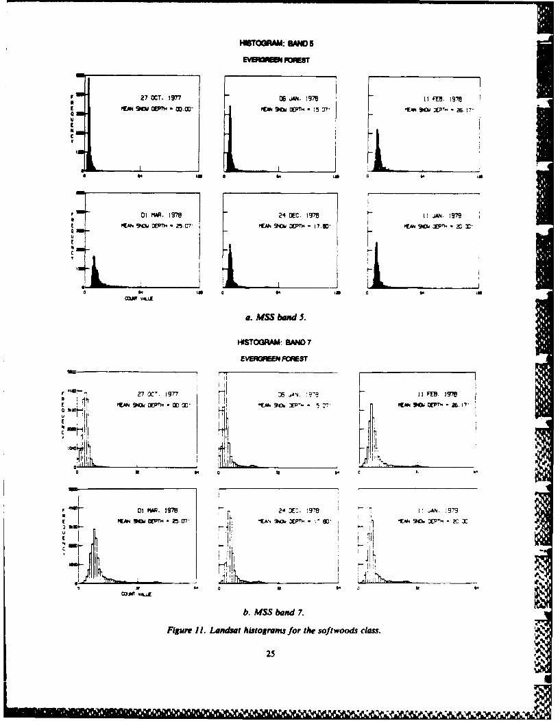
HISOGRAM: SANOS

2 7 OCT. 1977 105 ONI. 978 1 IFE9. 1978PO C " -0 c I P(N 9 TH - 15C7, - -94WOPT. - 26 17'

c

U

Vl MA. 197 X jDEC. '9-9l 1 JAN.B 97I"

.

c

F ~ ~ ~ ~ ~ a 01S W.n 1S.2 O, 9791

cope V*iix

Clb MSS. b97d 7.

Figure~~ I/ Ln9thitgrmsfr hesftooscln

I(,A~o~rEP~h.2~a7 2~ .981IN '

__ _ _ _ _ _ _ _ __ MI

~ I d

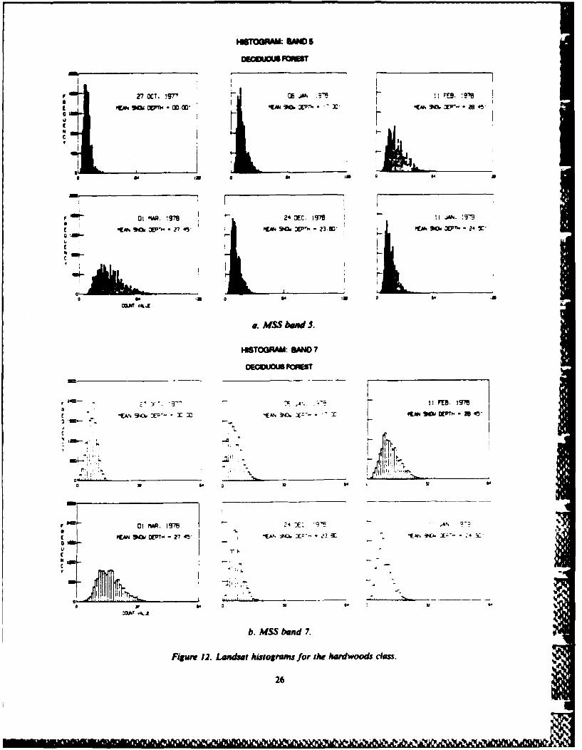
HITOAM: BAND$

27 OCT. 1977o 'A 1: FEB.g7

- 0

c

01A. !7 24 3~EC 1978 :1-!N

am

E I

3=- :'~'-o- 1

a= P". 19" 2' X: *'9'9 %-

~ ~ 9 MVT.,. c =I" - 27 45' 'CA 5P : EZ - 23 W. X; 3t' - '3Z*

v

I"1[(AA !.-?4 " ) j I' ""I -

0

b. MSS band 7. -

Figure 12. Landwet histograms for the hArdwoods clan . CAM

HITOMM @AM 5

27XT. !971

"EI1 E"-3 M. *CA93Et . 90-,. IC-

£7

l Mo. !9-0

a. MSS bend 5.

HIBTOORAM: WMd 7

IL

pIr01 MO. 1970 24 EC. 1'798 ' : AN. 9-

30 -r If SW U :se p92

b. hISS band?.

27 Z

Figaure ~ ~ ~ lwF% 13owdehuorasfrte-% ie foet9es ~

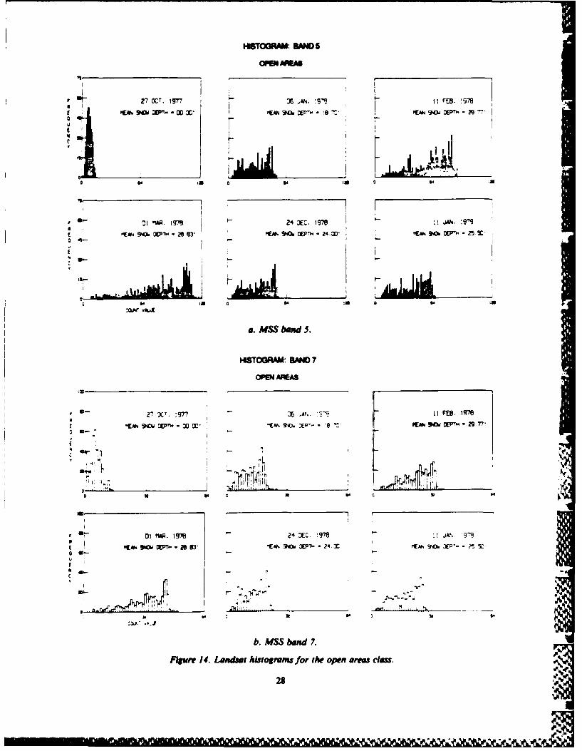
,ISTOORAM: 5 5

iap_

27 OCT. 19jr7 0 J . S i'? 1 EB. Ig"SS9"m X:1 -r " I WM . 9", X'- B .I 7C, ' PM9 OT- 29 7. "

SI II hi0 8 0 is a 0a

a-l 1 M 79 24 EC. Il 1S i

4L'3- LiP ,-

I

go-

a. MSS bad 5.

HISTORAM BAND 7

OMP WRM

27XT. !97 7 o I" s

aN

0f4 9 U 4 00 CCC N b6DP- e9 ~ 7

01 P~q 1978 24 OEC :78: ,A%.

,(C*O'SW ET..U2S 3'I4%9 h 3XPTN 24I O(M3 XP*- 2'

o -C-

U~b MSS bnd 7.~04

Figure 14. Landsat histograms for the open areas class.

HISTOGRAM: BAND 5WATER

=1 1 0 I n Fi

a27 OCT. 27nO A . :991 E.17

S0 1 nw , 1 " 24 OEC .1 78 11 JAN . 1

EC r

Nc

0 U

1 01 MAP._1___4___C.I I IA.:Il

2 2.Y

. MSS band 7.WAER

In-

2929

_ __i

b- .-$

bnd

Fiue! .LnUthsora sf rtewtrcas

- I,

Ht

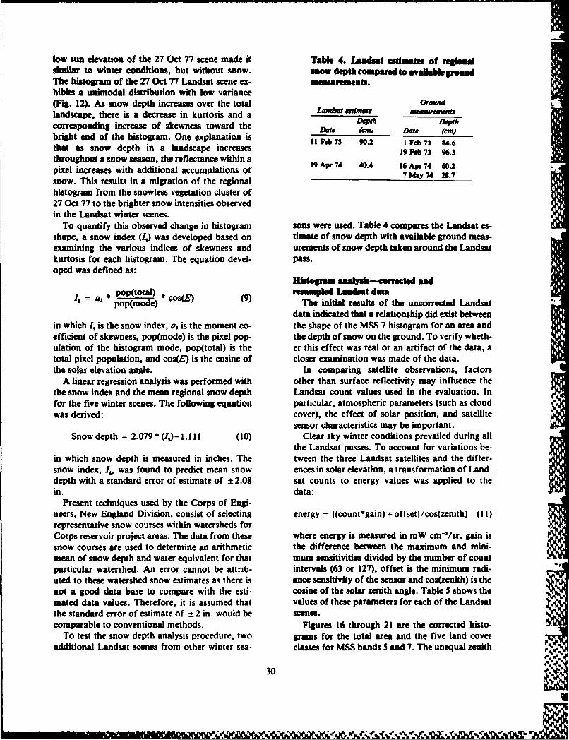
low sun elevation of the 27 Oct 77 scene made it Table 4. Lmdut edmat of rgionalsimilar to winter conditions, but without snow. mow depth compared to avalbdle gromThe histogram of the 27 Oct 77 Landsat scene ex- measarements.hibits a unimodal distribution with low variance(Fig. 12). As snow depth increases over the total GOYomdlandscape, there is a decrease in kurtosis and a aetate fika__ _mmD"M~h LeptWcorresponding increase of skewness toward the Date (CM) Date (CM)bright end of the histogram. One explanation isthat as snow depth in a landscape increases 19 Feb 73 96.3throughout a snow season, the reflectance within apixel increases with additional accumulations of 19 A774 40.4 16 Ap 74 60.2snow. This results in a migration of the regionalhistogram from the snowless vegetation cluster of27 Oct 77 to the brighter snow intensities observedin the Landsat winter scenes.

To quantify this observed change in histogram sons were used. Table 4 compares the Landsat es-shape, a snow index (IJ was developed based on timate of snow depth with available ground meas-examining the various indices of skewness and urements of snow depth taken around the Landsatkurtosis for each histogram. The equation devel- pass.oped was defined as:

Khtogrm mnuiyh-cowected nd1, = a, * pop(total) cos(E) (9) reuampled udsat data

pop(mode) The initial results of the uncorrected Landsatdata indicated that a relationship did exist between

in which I is the snow index, a3 is the moment co- the shape of the MSS 7 histogram for an area andefficient of skewness, pop(mode) is the pixel pop- the depth of snow on the ground. To verify wheth-ulation of the histogram mode, pop(total) is the er this effect was real or an artifact of the data, atotal pixel population, and cos(E) is the cosine of closer examination was made of the data.the solar elevation angle. In comparing satellite observations, factors

A linear regression analysis was performed with other than surface reflectivity may influence thethe snow index and the mean regional snow depth Landsat count values used in the evaluation. Infor the five winter scenes. The following equation particular, atmospheric parameters (such as cloudwas derived: cover), the effect of solar position, and satellite

sensor characteristics may be important.Snow depth = 2.079 * (IJ- 1.111 (10) Clear sky winter conditions prevailed during all

the Landsat passes. To account for variations be-in which snow depth is measured in inches. The tween the three Landsat satellites and the differ-snow index, I , was found to predict mean snow ences in solar elevation, a transformation of Land-depth with a standard error of estimate of ± 2.08 sat counts to energy values was applied to thein. data:

Present techniques used by the Corps of Engi-neers, New England Division, consist of selecting energy = [(count*gain) + offset]/cos(zenith) (11)representative snow courses within watersheds forCorps reservoir project areas. The data from these where energy is measured in mW cm'/sr, gain issnow courses are used to determine an arithmetic the difference between the maximum and mini-mean of snow depth and water equivalent for that mum sensitivities divided by the number of countparticular watershed. An error cannot be attrib- intervals (63 or 127), offset is the minimum radi-uted to these watershed snow estimates as there is ance sensitivity of the sensor and cos(zenith) is thenot a good data base to compare with the esti- cosine of the solar zenith angle. Table 5 shows themated data values. Therefore, it is assumed that values of these parameters for each of the Landsatthe standard error of estimate of ± 2 in. would be scenes.comparable to conventional methods. Figures 16 through 21 are the corrected histo-

To test the snow depth analysis procedure, two grams for the total area and the five land coveradditional Landsat scenes from other winter sea- classes for MSS bands 5 and 7. The unequal zenith

30

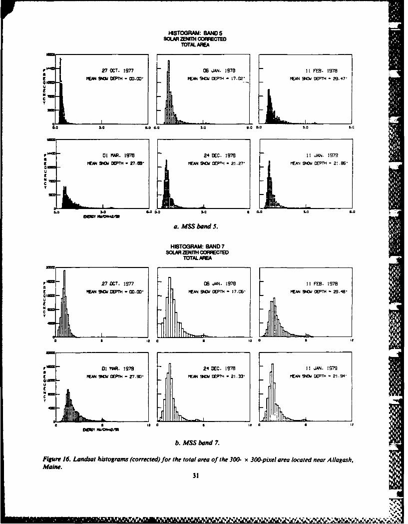
HISTOGRAM: BAND SSOLAR ZNTH CORRECTED

TOTAL AREA

27 OCT. 1977 05 JAN. 1975 11 FEB. 1978SMENSNOW DEPTH - 30,* ENO DE 0PTH - 17.02 EANO DEPTH - 29.47"

0u

C 7y

&.0 .0.0 0.0 .0 l.O 0.0 3.0 6-C

o m IFlom - 01 MAR. I9SM 24 D3EC- 1978 -I 11 N. IS793

E WAN S NOM - 27. ee SNOW ' - 21.27 AN SNOW DEPTH 2' "

N7=y

0.03.06.0.0 M. S .6. .

o,,,- -- -- _

a. MSS band 5.

HISTOGRAM: BAND 7SOLAR ZENIH CORRECTED

TOTAL ARE

FF 27DCT. 1977 06 JAN. 1970 11 FED. 1978

E MEAN 9" ETH - 00.00 HE DEPTH - 17. 0'EAN"I 9M DEPTH - 29,48'

o AR 1-

MEAN SNOW DPTH - V'.9M" MEAN SNO DEPTH - 21.33' ME SNOW3 DEPTH -21.94"

U

C

ME, L I I I I* 0L.. - £ . ,i

0 '

b. MSS band 7.

FIgure 16. Landsat histograms (corrected) for the total area of the 300- x 300-pixel area located near Allagash,Maine.

31

11,110 ,1111 %M 111 'llIN G --- ---

HISTOGRAM: BAND 5SOLAR ZENIH CORRECTED

EVERGREEN FOREST

l LF 27 OCT. 1977 -6 JAN. *15 1! FEB. 978

E27 NWDET 000 A -OCT.H 15-7 FA 0,J DEPTH - 26.17*

1r,V I

0.0 3.0 6.0 0.0 3.0 6.0 0.0 3.0 6.3

F !2m 01 MAR. 1978 24 DEC. I78 - I ,JAN. 1S79

E MAN NOg IPTH - 25, 07" MEM 5U DEPTH - 17.8Y I C_4 , -

- I

0.0 3.0 6.0 0.0 3.0 6.0 0.0 3.0 6.0

(DIM'f MW/0%-*2/sl

a. MSS band 5.

HISTOGRAM: BAND 7SOLAR ZENITH CORRECTED

EVERGREEN FOREST

F 41- 27 OCT. 1977 -0 JAN. iS78 II FEB. 1978

A C7 M A 9 EP H 6 . 7

E MANA1 9 T DEPTH - 0?.0." 00SN0'E -SNOW DEP

U

C

o 63 60 0 6

F 01 MAR. 1978 24 DEC. 1978 II JAN. 1979

FigN9 DETH - 2s7t g rm - 1 (E 0 MAN 9aftwooH - "_3.0 31M2U

10C

0612 0 0 6 0

b. MSS band 7.Figure 17. Landsat histograms (corrected) for the soft woods class.

32

Jp *

HISTOGRAM: BAND 5SOLAR ZENrTH OORECTED

DECCUOUS FOREST

F 27 OCT. 1977 :)6 AN. '!.. IItB I7

MEAN SiU DEPTH - 00.00' 'ff, 9JO. DP - 7X M 9 = - 2..45

rram -

0.0 3.0 6.0 0.0 3.0 5.0 0.0 3.0 6.0

F am, 01 MAR. 1978 2'DCC. 1978 11 JAN. I7

E MFAN S -DEPTH - 27.45' MEAN 5" DEPTH - 23.B[- W-9. 5,';- Z:T- 24.50"

U

C7

4M=--

.0 3.0 60 0. 3.0 60 00 3.0 6.0

a. MSS band 5.

HISTOGRAM: BAND 7SOLAR ZENITH CORFECTED

DECIDUOUS FOREST

F * 27 OCT. 1977 OE JAN. 1978 11 FE-. 1976

E MEAN SNOW DETH - 001.CU* PEAN 30w DPTH - 17.U MAN 9C61 DF7H -2_.450 ,w

UE

N [am-C

y

F 201 C MAR. 1978 24 DEC. 19718 11 JAN. !7n

* a 6 6

E MEASNODEPH- 27.45' E \()W DE0PTH -238' MEtA 9" OEPTH 24 50

U

C40 a 12 a 6 2 062

b. MSS band 7.

Figure 18. Landsat histograms (corrected) for the hardwoods class.

33

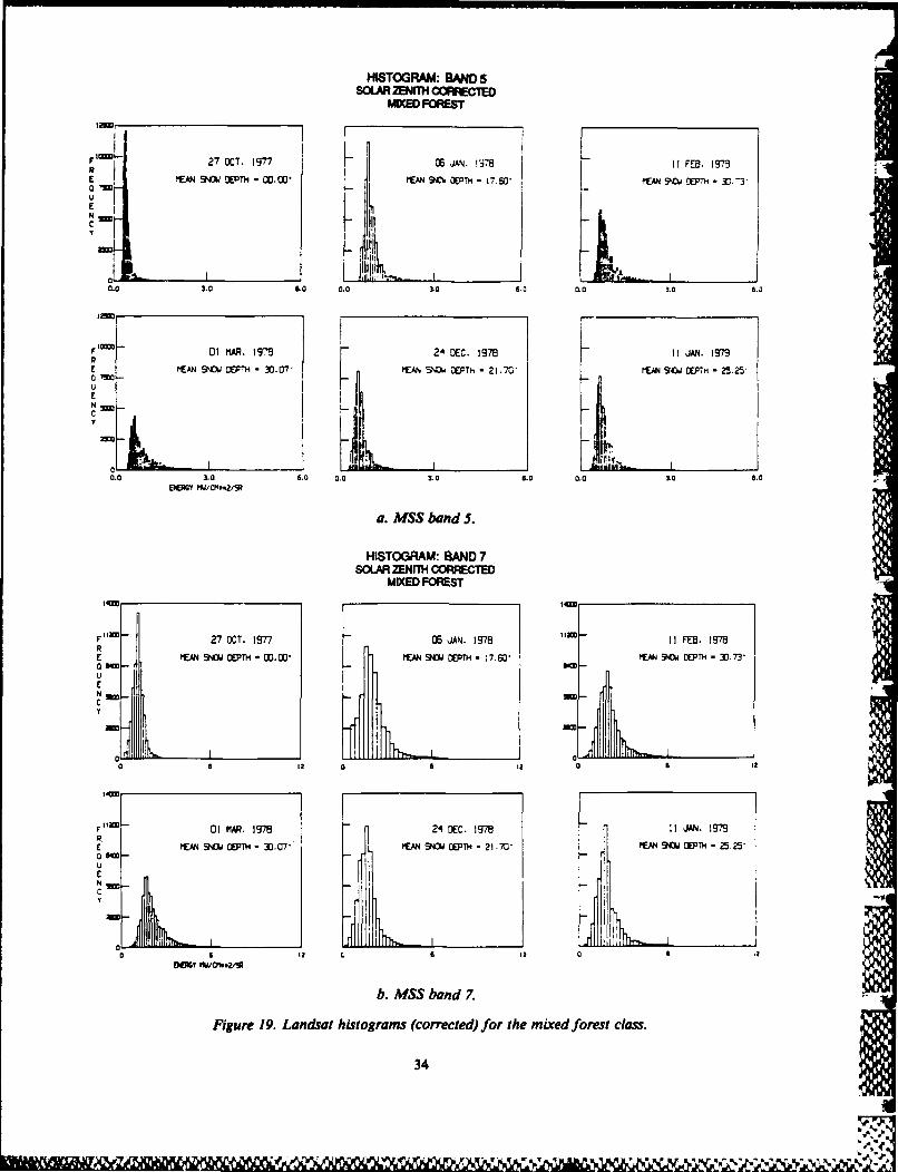
HISTOGRAM: BAND 5SOLAR ZENTH CONRECED

MIXED FOREST

2 27 OCT. 1977 E JAN. !'78 11FEB. 197EAN Ism AN = DEPTH - 17." 6' 91C DEPTH- 30.-3-'

UEl f

NII

CLO 3.0 6.0 0.0 .0 0- 00 1.0 6.3

Fl0 C1 MAR. I'S 24 DEC. 1978 11 JAN. IM

E~ MA N EPTH4 -30(7' PEAJ. 5S,- DEPTH - 21.70' M. ,WI Rm-2-5

N

0.0 3.0 5.0 0.0 3.0 6.0 0.0 310 6.0

a. MSS band 5.

HISTOGRAM: BAND 7SOLAR EiNfTH CORRECTEDMIXED FOREST

F 27 OCT. 1977 06 JAN. 1978 11 FEB. ISM7RE MAN 9 DETH - Inr0. MIAN SNOW DPTH - 17.6* 90d UlT' =.73"

U

E N-

bMbd0 1 2 0 6 12060

Fi"amL0 1 MAR. I78 24 DEC. 1978 11 JAN. IM

UENC sy -$

0 S ? CI

L

b. MSS band 7.

Figure 19. Landsat histograms (corrected) for the mixed forest class.

34

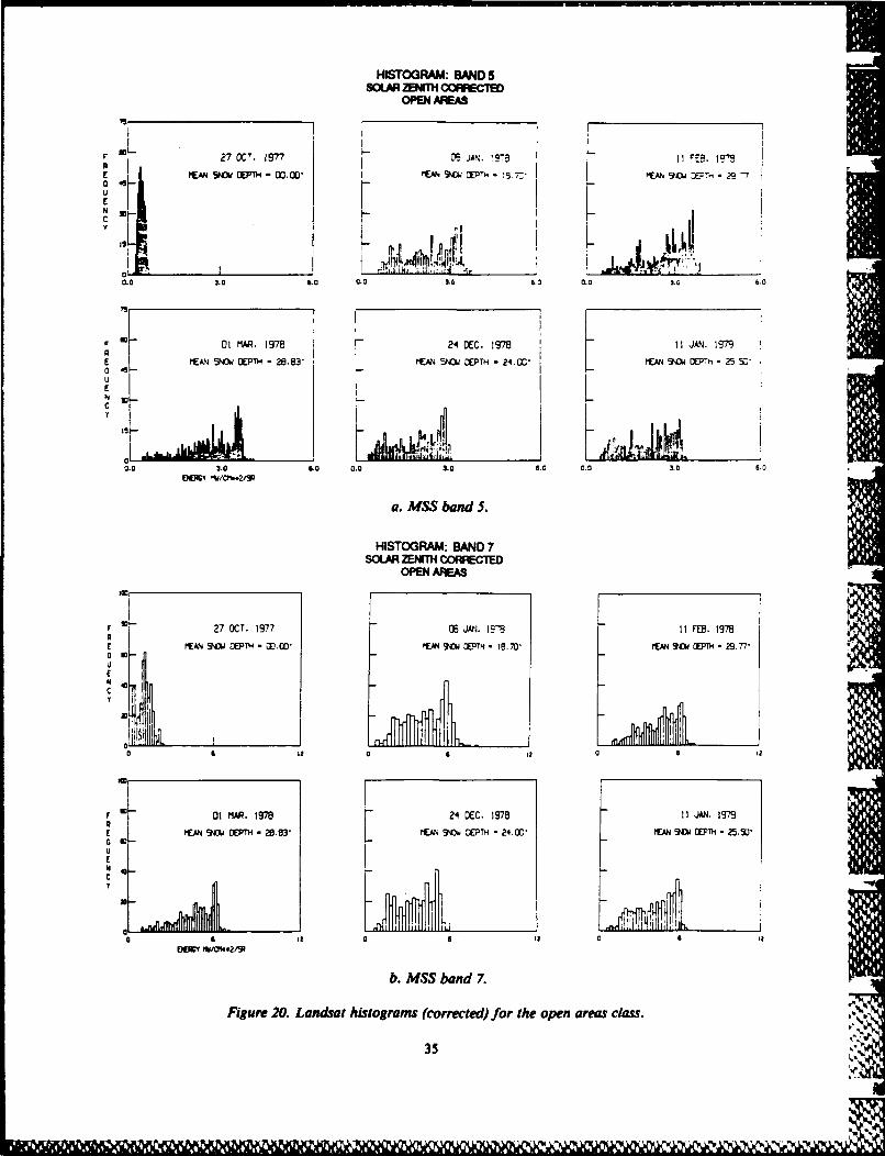
HISTOGRAM: BAND 5SOLAR ZENITH OORRCTED

OPEN AREAS

27 OCT. 1977 KA%, 1- L1 CEO 19

y I .. H003 00.0 3.0 6.0 c.0 30 6.0

v 27 OCTMA. 1978 24 JAC. 1978 11 JAN. 1978

E PfAN 9O DEPTH - 288*MM 5\43 OEPTH - 2.OC'Pf 9O" DETH - 25 50OWUE

CI

y

Q0 6 . 03 0 £ 0 6.0 (.

F 27 OCT. 1977 06 24DE. 199 11 JEB. 1978

E EA 940w DEPTH - 0000 EN 90 DEPTH 10. 70M 9OW OPTH - 2.70 --U

U

b. MSS band 7.

Figure 20. Landsat histograms (corrected) for the open areas class.N

I e

HISTOGRAM: BAND 5SOLAR ZENITH COWFECIED

WATER

27 OCT. 1977 06 JAN. 1979 I1 FEB. 197e

UEIFI

r.f0O 00 3.0 6.0 0.0 3.0 6.0

F 0 1 MAR. 1978 - 24 DEC. 1978 II JAN. 1979R

E

0 --

NC

y

.0 0.0 3,0 80 00 3,0 1,,

a. MSS band 5.

HISTOGRAM: BAND 7SOLAR ZNITH CO CTED

WATER

F 27 OCT. 1977 06 JAN. 1978 I FEB. 1978

£o -UCN

C" 4.y

a

a It 65 65

F - 01 iAR. 1978 24 DEC. 19"5 11 JAN. 1979

R0

UENC

Y ,v

i0 0 It2

b. MSS band 7.

Figure 21. Landsat histograms (corrected) for the water class.

36

&MMUC-

Tal S. Saiaw pwoars md le the cwmthm of

DW& ASS5 Q SS 3 M e tS 7 Canit ok

27 Oct 77 0.0134 0.0603 0.06 0.11 0.39076 ja 78 0.0134 0.0603 0.06 0.11 0.2079If Feb 78 0.0134 0.0603 0.06 0.11 0.3256

1 Ma 78 0.0134 0.0603 0.06 0.11 0.438431 May 78 - - - --

24 Dec 78 0.0139 0.0603 0.03 0.03 0.2588II Jan 79 0.0139 0.0603 0.03 0.03 0.2756

angle of the various Landsat scenes resulted in un- bands there is a strong similarity in the histogramsequal radiance levels between consecutive count on all snow-covered days.values for each scene. For example, changes in one Histograms for the corrected and resampledcount value in the MSS 7 uncorrected data for 6 MSS 7 data for the total area and the forestedJan 78 and I Mar 78 resulted in radiance changes classes did not change significantly with changesof 0.29 and 0.138 mW cm-/sr, respectively, in the accumulated snow depth (Fig. 22-25). A

A resampling scheme was applied to correct for quantitative evaluation of the histograms wasthis radiance interval variation. The histograms made and the results are shown in Tables 6 and 7.were resampled to the energy levels of 6 Jan 78, Statistics on the mean, median, mode, standardthe Landsat date with the lowest solar elevation deviation, first and third quartile, 10th and 90thangle. For 6 Jan 78 the following energy values percentile, five indices of skewness, and three in-correspond to the MSS 7 count levels: dices of kurtosis are presented. The radiance inter-

vals between histogram levels are equal to 0.064MSS 7 count level: and 0.29 mW cm-'/sr for MSS bands 5 and 7, re-

0 1 2 3 4 ... 63 spectively. For the five snow days shown, threewere observed with Landsat-2 (6 Jan 78, 11 Feb

Radiance (mW cm-/sr): 78, and 1 Mar 78), while two days were observedwith the Landsat-3 satellite (24 Dec 78 and 11 Jan

0.53 0.82 1.11 1.40 1.69 ... 18.80 79). Although differences in sensor gain and offset

were taken into consideration during the correc-For example, for the 1 Mar 78 scene, count level a tion process, the Landsat-3 observations showcorresponds to a radiance value of 0.94 and has a larger energy values.pixel population of 1750. Count level 5 is then re- Table 8 shows the average snow depth for eachsampled by weighting between levels 0.82 and 1.11 land cover class and the total. These values weremW cm-2/sr and the pixel population is calculated determined from the snow course measurementsusing the following two equations: taken during the time of the Landsat overpasses.

The 31 May land cover classification was used

poPo.s2 = 1750 * 1.11-0.94 = 1026 (12) to provide a mask with which the histograms of1.11-0.82 Landsat data could be evaluated for each of the

land cover classes. Histograms for the forestedpop,.,, = 1750 * 0.94-0.82 = 724. (13) landscapes, which predominate in the region, dis-

1. 11-0.82 play characteristics similar to the total areas (Fig.

This procedure is repeated for each count level of 22-25).this croeure irpeted histogr for deh othe lel oThe histogram statistics for the three forestthe corrected histogram to derive the resampled types and the total area are similar for the threehistogram, winter Landsat-2 dates (Tables 6, 7). The meas-

Figures 22 through 27 show the corrected and ures of central tendency (mode) and the standardresampled histograms for MSS bands and 7 for deviation (s) are similar. Means, quartiles, andthe total study area and the individual land cover percentiles show differences between scenes lessclasses. Within each land cover class for both than the radiance intervals between histogram

37

°I

HISTOGRAM: BAND 5SOLAR ZWTH OMRECIWD & RAAwLW

TOTAL AE

27C IT. 1977 06 JAN. 1978 11 FEB. 1975

PIE SWMPH-.(0'ME MDI - P.0* EA 9"d DETH 294

C

y

0 •a .

F D! fW. 197 24 JEC. 1975 11 ,,N. 1979

at=0'-UE

C

a. MSS band 5.

HISTOGRAM: BAND 7SOL.ARq ZENITH OOR-T & R3ESAWL0-E

TOTAL AREA

F34 - 27 OCT. 1977 06 JAN. 1978 11 FEB. 1978

M~NSd~Ph-~PEAN SNOW DEPTH - 17.02* MEAN SNOW DEPTH - 29.47-E MEAN SNO DEPTH -00.00'

0.0 3.0 5.0 0.0 3.0 6.0 0.3 6.0

F21= Ol MAR. 1978 24 DCC. I978 II JAN. 7TS

E mEAN 9M EPTH - 27.88" MA' SNOW DEPTH - 21.27' - A. 9 [Ph - 2."

0.0 -31-0 LO 0.0 3.0 6.0 0.0 3t.0 1.0

b. MSS band 7. .

Figure 22. Landsat histograms (corrected and resampled) fo h oa 0-x 300-pixel area lctdna

Aliagash, Maine.

01638

U

HISTOGRAM: BANDSSOLAR ZENrTH OORRCTED & RESAWI.ED

EVEWEE FOREST

f27 OCT. 1977 OE AP4. 1979 11 FEB. !9

C PI tAt SOW DEPTH - 0:.007 Pl/m EPTH - IC" % 9 OEPT. - 2, 17-

£ I I

LO 3.0 6.0 0.0 3.0 6.0 0.0 3.0 0

F 0 MIAP. J1378 r 24 DEC. IM7 I I JAN. :979

0 .0

HISTOGRAM: BAND 7SOLAR ZENI1TH CO)RREED & RESAMPLED

FOREST

C

NL

Lr

Imn- l7 OT. h7- I1 JAN I I , F.-.E7

0.0 3 6.0T00 - 41.0 0 3." ,

l SO MAR. R978 24 DEC. 1878 1I JAN. &87

E PE[, I:T .""IIAN SNOW DEPTH -0 M'EAN 9"O DEP-7H -!5.I7"

0 4MU

E

NCI

b.MSS band 7.Figure 23. Landsat histograms (corrected and resampled) for the softwoods class.': _

39

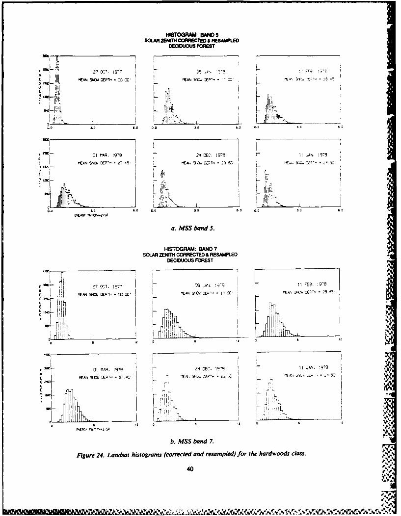
HISTOGRAM: BAND 5SOLAR ZWdH CORRECTED & R ALED

0EClDJOUJS FOR:EST

I P6L 'i l - - ..... *

r 3.0 4.0 0.0 6- L .0 )t

DI O MA!R. 97 .4DC 97 l AN. ) 7

1 a=7 14~C 27T9' 9

P'EA 93 O "- - 2, 45" ' PMA 5W. X- - M _. 3.-. . -5 P-

U

N

A, i

0 . 30 6.0 00 0 1.O 0,0 '.0 LV

(610

a. MSS band 5.

HISTOGRAM: BAND 7SOLAR ZENfTH CORRECTED & RESAMPLEDDECIjOUS FOREST

F Wl:27 T T. 197 Z- 11 .,A. ;9'9

E MEAN SNOW ANS=O - *1X

C" I'D "F 0 MAR. :97R 21 DEC. 19' 11 .jAN. lcz1

p 0 - 2- 45- 2- , I'5 . -

J2 1 !It I I - I I

NN0 s2 0 6 2 0 6 z0

b. MSS band 7.

Figure 24. Landsat histograms (corrected and resampled) for the hardwoods class.

40

AA

vp .

H X*A: ON O 5

SOLARWTHORCEDA RAAMLED

[ (M 90 Z ?~ *[nt 0[ 3" "(M.* t7 X=" - ", lE . ia. . V-* 2&O F ,IW

0.

0A m3

0 :i

E Cwt ", O [EP- - 3[= 7, " ;E,,.,.-,,: "Vi. 5 :- - .

U

a. M S 15.5.

HISTOGRAM: BAND 7

Dl AR . 24lil , C.C _ 'e l1.JAN. '.. ,

27 OC .17I6 jr-I-;"9 "-C SAN 9". OPN' - 0000 K. 9"J Xcj -' 3C.

o EA 940 :)P

01 MAP . 1979 24 DEC. 19"15- 11 JAN,. !9-

U I pfo PEAN S DEPT- - 3 ' P , 3 : '

- -0SP --

b. MSS bond 7.

Figure 25. Landsat histograms (corrected and resampled) for the mixed forest class. %41.

HISTOGRAM: BANDSSOLAR WIa h O1ECD & RSAL

OPE AREA

r OCT. 197 - 06 A,;. ,- ' Fr. F 1-0

, 1 M AP. 1 24 D C . ! M 11 JN . !97

MENSO PH 2 L- OtH9c ,Cp-. 57r- Z5 30

4'_ _ _ _ _ _ _ _ _ _ _ _ _

0.0 & 0 00 1"0 hO O 0 hO4.

0 _ _ _ I 0 Vr

0 1W ". ,1l.00 0. 1.

a. MSS band 5.

HISOGRAM: BAND 7SOLAR ZENITh OORREWED A RSAWLED

OPEN ARAS

I. I

27OCT. 1977 K JAN. !9'79F Fdt. 1,-9

EWEN 90d DPTm - 000-PA 9CW OTH -'~ ~I sprl cElrrl -

0~1 0 I0II

0 1 MP 1 4 C 1

b. MSS band 7.Figure 26. Lunldsat histograms (corrected and resampled) for the open aesc/as

42b

HISTOGRAM: BA SSOLAR ZWTH CORECTED & RESAMLED

WATE

Z7 OCT. 1977 05 , 9"Z

0.0 0.0 La 6. 3.0

b 01 MP. Ism 214 DEIC. 19797 11 JAN. 1979

a. MSS band5..IsE0 qU

-

o D0

pV - 01 MAR. 19'78 -- 4 DEC¢ 1978 II JAN. 1975 1

N

b. MSS band 7.

F igure 27. Landuat hstogramst (corrected and resampled) for the water c/ass. '

4,".

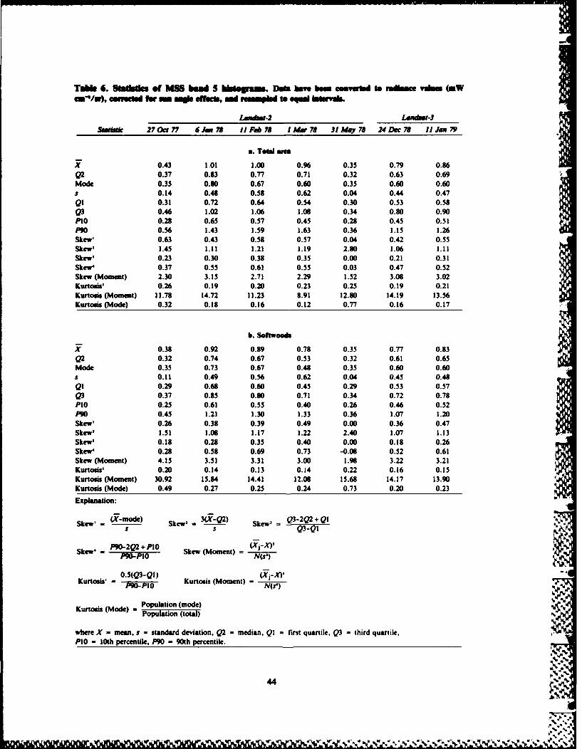
TAle 6. Shmtmt of MSS buid 5 htogrms. Daf bm bm coavel toWraim abon (Win"/uw, ewndi orm b .dfelketo d reemupu to @ql bharvk.

Lan dia-2 LANdurt-3

SaOb* 27 Oct 77 6)., 78 11 Fab 78 Mar 78 31 M 78 24 Dec 78 11 Jan 79

a. Toal ars

X 0.43 1 01 1.00 0.96 0.35 0.79 0.86Q2 0.37 0.33 0.77 0.71 0.32 0.63 0.69Mode 0.35 0.80 0.67 0.60 0.35 0.60 0.60s 0.14 0.48 0.58 0.62 0.04 0.44 0.47Q! 0.31 0.72 0.64 0.54 0.30 0.53 0.58Q3 0.46 1.02 1.06 1.0 0.34 0.80 0.90PlO 0.28 0.65 0.57 0.45 0.28 0.45 0.52P90 0.56 1.43 1.59 1.63 0.36 1.15 1.26Skew. 0.63 0.43 0.58 0.57 0.04 0.42 0.55Skew, 1.45 1.21 1.21 1.19 2.80 1.06 1.11Skew' 0.23 0.30 0.38 0.35 0.00 0.21 0.31Skew4 0.37 0.55 0.61 0.55 0.03 0.47 0.52Skew (Moment) 2.30 3.15 2.71 2.29 1.52 3.08 3.02Kurtouis 0.26 0.19 0.20 0.23 0.25 0.19 0.21Kurtouis (Moment) 11.78 14.72 11.23 8.91 12.80 14.19 13.56Kurtoms (Mode) 0.32 0.18 0.16 0.12 0.77 0.16 0.17

b. Softwoods

X 0.38 0.92 0.89 0.78 0.35 0.77 0.83Q2 0.32 0.74 0.67 0.53 0.32 0.61 0.65Mode 0.35 0.73 0.67 0.48 0.35 0.60 0.60s 0.11 0.49 0.56 0.62 0.04 0.45 0.48QI 0.29 0.68 0.60 0.45 0.29 0.53 0.57Q3 0.37 0.85 0.80 0.71 0.34 0.72 0.78PlO 0.25 0.61 0.55 0.40 0.26 0.46 0.52POO 0.45 1.21 1.30 1.33 0.36 1.07 1.20Skew' 0.26 0.38 0.39 0.49 0.00 0.36 0.47Skew, 1.51 1.06 2.17 1.22 2.40 1.07 .13Skew' 0.18 0.28 0.35 0.40 0.00 0.18 0.26Skew4 0.28 0.58 0.69 0.73 -0.06 0.52 0.61Skew (Moment) 4.15 3.51 3.31 3.00 1.98 3.22 3.21Kurtois' 0.20 0.14 0.13 0.14 0.22 0.16 0.15Kurtods (Moment) 30.92 15.84 14.41 12.08 15.68 14.17 13.90Kurtouis (Mode) 0.49 0.27 0.25 0.24 0.73 0.20 0.23

Explanation:

Skew' -(-mode) Skew' 3(X-Q2) Skew' Q3-2Q2 + QIs s Q3-Ql

Skew P9-2Q2 + PO Skew (Moment) = _(sj) _

o.5(Q3-Ql) (X.-X). -Kurtois' = - Kurtouis (Moment) = N()

Population (mode)Kurtosis (Mode) - Population (total)

where X - mean, s = standard deviation. Q2 = median. QI = first quartile. Q3 = third quartile.PIO = 10th percentile, P90 90th percentile.

p% '' .a .. .%

Pa.

Table 6 (cont'd). Statistics of MSS band S histograms.

Landrot-2 Landsat.3Statistic 27 Oct 77 6 Jan 78 11 Feb 78 1 Mar 78 31May 78 24 Dec 78 11 Jan 79

c. Hardwoods

X 0.52 1.12 1.15 1.19 0.36 0.81 0.89Q2 0.47 1.00 1.03 1.08 0.32 0.71 0.78Mode 0.48 0.99 0.80 0.99 0.35 0.60 0.60s 0.14 0.35 0.42 0.43 0.04 0.29 0.32QI 0.40 0.84 0.80 0.83 0.30 0.56 0.62Q3 0.56 1.24 1.34 1.40 0.34 0.93 1.01PlO 0.34 0.73 0.67 0.67 0.29 0.48 0.54P90 0.66 1.57 1.71 1.74 0.36 1.18 1.27Skew, 0.33 0.37 0.85 0.47 0.15 0.69 0.89Skew' 1.08 1.03 0.90 0.77 2.88 1.04 1.02Skew' 0.05 0.21 0.15 0.14 0.00 0.23 0.18Skew4 0.16 0.38 0.32 0.24 0.16 0.35 0.34Skew (Moment) 1.37 1.64 1.17 0.91 9.63 1.36 1.51Kurtois' 0.25 0.24 0.26 0.27 0.26 0.26 0.27Kurtouis (Moment) 7.28 9.79 4.82 3.98 11.91 6.35 7.80

Kurtosis (Mode) 0.22 0.12 0.09 0.08 0.81 0.12 0.12

d. M114d forestX 0.43 0.94 0.92 0.87 0.35 0.72 0.80Q2 0.37 0.81 0.75 0.68 0.32 0.62 0.67Mode 0.35 0.80 0.67 0.60 0.35 0.60 0.60s 0.13 0.35 0.43 0.48 0.03 0.31 0.35QI 0.32 0.72 0.64 0.54 0.30 0.51 0.57Q3 0.44 0.97 0.91 0.96 0.34 0.76 0.85PlO 0.29 0.65 0.57 0.46 0.28 0.44 0.50P90 0.54 1.21 1.35 1.42 0.35 1.01 1.13Skew' 0.61 0.41 0.58 0.56 0.01 0.38 0.57Skew' 1.43 1.08 1.16 1.19 3.06 1.02 1.09Skew' 0.19 0.26 0.31 0.33 0.00 0.17 0.25Skew' 0.36 0.41 0.52 0.53 -0.03 0.37 0.44Skew (Moment) 2.61 3.39 2.80 2.39 0.55 2.93 2.98Kurtosis' 0.25 0.22 0.22 0.22 0.27 0.21 0.22Kurtosis (Moment) 13.70 19.10 13.34 10.26 6.56 15.84 15.44Kurtosis (Mode) 0.03 0.20 0.17 0.15 0.78 0.16 0.18

e. Open freas

X 0.46 2.2! 3.80 3.85 0.47 1.92 2.11Q2 0.42 2.24 2.40 2.48 0.45 1.97 2.22Mode 0.41 3.41 3.54 3.54 0.48 2.84 3.16s 0.10 0.86 1.71 1.69 0.07 0.77 0.84Q1 0.35 1.41 1.71 1.86 0.40 1.20 1.35Q3 0.51 3.05 2.86 2.91 0.51 2.52 2.85PlO 0.30 1.00 1.13 1.09 0.37 0.78 0.80P90 0.57 3.33 3.04 3.16 0.58 2.84 3.11Skew, 0.49 -1.34 0.16 0.18 -0.15 -1.20 -1.25Skew' 1.17 0.03 2.47 2.43 0.55 -0.19 -0.39 %Skew' 0.09 -0.02 -0.20 -0.19 0.09 -0.16 -0.16 .Skew, 0.09 -0.07 -0.33 -0.35 0.18 -0.16 -0.23Skew (Moment) 0.19 -0.17 -1.26 -1.29 1.10 -0.25 -0.30Kurtosis' 0.28 0.35 0.30 0.25 0.27 0.32 0.33Kurtosis (Moment) 2.30 1.69 1.76 1.88 3.20 1.77 1.79Kurtosis (Mode) 0.24 0.06 0.08 0.10 0.33 0.06 0.06

45

A.. . . .

Tu 6 (mot'd). Smsla of MSS bemd 5 bbtogrms. Deft he bn .cOeed to mbmm vI(=W '/Iw), f I hr dibelh , ari ruampi to eqa inksev .

Landsat-2 Landsat-3

statitic 27 Oct77 6 Jan 78 11 Feb 78 1 Mar 78 31 May 78 24 Dec 78 11 Jan 79

f. Waler

0.37 2.57 3.07 2.92 0.35 2.33 2.46Q2 0.31 3.03 3.45 3.38 0.31 2.66 2.83Mode 0.29 3.41 3.67 3.60 0.35 2.97 3.16s 0.09 1.02 0.87 0.93 0.06 0.81 0.89QI 0.27 1.55 2.74 2.46 0.28 1.70 1.76Q3* 0.38 3.37 3.61 3.55 0.34 2.94 3.13PIO 0.24 0.92 1.52 1.27 0.25 0.92 0.91P90 0.47 3.54 3.70 3.61 0.39 3.05 3.25Skew' 0.92 -0.33 -0.69 -0.73 0.03 -0.78 -0.78Skew' 1.80 -1.38 -1.32 -1.48 1.90 -1.22 -1.24Skew' 0.18 -0.63 -0.63 -0.69 -0.02 -0.55 -0.56Skew4 0.36 -0.61 -0.77 -0.81 0.08 -0.64 -0.64Skew (Moment) 1.26 -0.56 -1.40 -1.29 1.83 -0.83 -0.82Kurtosis, 0.25 0.35 0.20 0.23 0.20 0.29 0.29Kurtosis (Moment) 4.52 1.86 3.91 3.42 8.88 2.36 2.30Kurtosis (Mode) 0.36 0.10 0.13 0.18 0.55 0.12 0.12

Table 7. Statistics of MSS band 7 hitoplams. Data have be conavered to raiace values (=Wm-/u), eorecad for m a& effet, ma rempls to equal uterva.

Landsat-2 Landsat-3

Statistic 27 Oct 77 6 Jan 78 11 Feb 78 1 Mar 78 31 May 78 24 Dec 78 11 Jan 79

a. Total srea

X 1.24 2.29 2.32 2.30 1.90 1.88 2.07Q2 1.06 1.80 1.89 1.85 1.72 1.59 1.71Mode 1.10 1.67 1.96 1.67 1.67 1.67 1.67s 0.40 1.07 1.08 1.07 0.52 0.86 0.95QI 0.83 1.40 1.50 1.45 1.37 1.22 1.36Q3 1.34 2.41 2.50 2.57 2.14 1.96 2.20PiO 0.59 1.05 1.19 1.16 1.14 0.90 1.10P90 1.62 3.30 3.51 3.52 2.48 2.72 3.02Skew' 0.35 0.49 0.33 0.58 0.44 0.25 0.42Skew' 1.33 1.11 1.19 1.25 1.05 1.03 1.16Skew' 0.09 0.20 0.21 0.28 0.10 0.01 0.18Skew' 0.08 0.33 0.39 0.42 0.14 0.25 0.37Skew (Moment) 0.60 1.91 1.84 1.65 0.09 1.93 2.03Kurtosis' 0.25 0.22 0.21 0.24 0.29 0.20 0.22Kurtosis (Moment) 3.88 8.05 7.14 6.12 2.73 8.33 8.39Kurtosis (Mode) 0.31 0.19 0.20 0.20 0.21 0.21 0.22

Explanation:

Skew'= (X-mode) 3(j'-Q2) Q3-2Q2 + QISe'-Skew' : Skew's s Q3-QI

Skew' = P90-2Q2 + PO Skew (Moment) = N(s')P90-PlO

0 5(Q3-Q1) (X-X).Kurtois' = Po-PO Kurtosis (Moment) N(s')

Kurtois (Mode) - Population (mode) OV

Population (total)

where Y - mean, s - standard deviation, Q2 = median, QI = first quartile, Q3 = third quartile, IPlO - 1Oth percentile, P90 - 90th percentile.

46

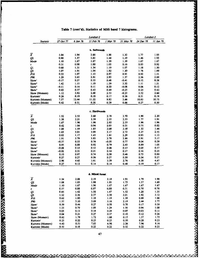
7q

Table 7 (cont'd). Statistics of MSS band 7 histograms.

Landsat-2 Landsat-3

Statistic 27 Oct 77 6 Jan 78 11 Feb 78 1 Mar 78 31 May 78 24 Dec 78 11 Jan 79

b. Softwoods

X 1.04 1.94 2.00 1.88 1.32 1.77 1.93Q2 0.90 1.57 1.61 1.44 1.19 1.46 1.93Mode 1.10 1.67 1.67 1.39 1.39 1.67 1.67

0.31 0.98 1.00 1.03 0.16 0.83 0.92Qi 0.68 1.31 1.34 1.19 1.07 1.18 1.30Q3 1.07 1.91 1.94 1.82 1.30 1.78 1.89PIO 0.53 1.07 1.13 0.97 0.91 0.92 1.11P90 1.29 2.65 2.81 2.83 1.37 2.36 2.69Skew' -0.17 0.27 0.33 0.48 -0.41 0.12 0.28Skew2 1.42 1.15 1.19 1.29 2.32 1.11 1.21Skew' -0.11 0.14 0.11 0.20 -0.08 0.06 0.12Skew' 0.03 0.37 0.43 0.49 -0.25 0.25 0.43Skew (Moment) 1.12 2.82 2.68 2.53 -0.23 2.52 2.60Kurtosis' 0.26 0.19 0.18 0.17 0.26 0.21 0.19Kurtosis (Moment) 7.57 12.44 11.22 9.82 3.66 10.83 10.73Kurtosis (Mode) 0.42 0.31 0.28 0.29 0.66 0.27 0.30

c. Hardwoods

X 1.52 2.52 2.68 2.78 2.70 1.99 2.20Q2 1.38 2.21 2.39 2.55 2.53 1.77 1.91Mode 1.67 1.96 1.96 2.82 2.53 1.96 1.96s 0.42 1.04 0.94 0.85 0.21 0.75 0.82QI 1.08 1.59 1.85 2.00 2.38 1.32 1.46Q3 1.65 3.01 3.09 3.17 2.72 2.27 2.55PlO 0.83 1.17 1.45 1.61 2.29 0.93 1.13P90 1.91 3.79 3.83 3.78 2.86 2.91 3.17Skew' -0.37 0.53 0.76 -0.05 0.77 0.04 0.29Skew' 0.95 0.88 0.92 0.79 2.43 0.89 1.05Skew' -0.08 0.13 0.12 0.06 0.13 0.05 0.17Skew" -0.02 0.21 0.21 0.14 0.17 0.16 0.23Skew (Moment) 0.10 0.87 0.74 0.58 0.46 0.75 0.89Kurtosis' 0.27 0.27 0.26 0.27 0.30 0.24 0.27Kurtosis (Moment) 2.96 4.62 3.61 3.29 2.76 4.20 4.47Kurtosis (Mode) 0.27 0.12 0.14 0.14 0.48 0.19 0.17

d. Mized forest

X 1.24 2.06 2.19 2.18 1.91 1.79 1.98Q2 1.08 1.83 1.88 1.81 1.75 1.57 1.69Mode 1.10 1.67 1.96 1.67 1.67 1.67 1.67s 0.37 0.88 0.87 0.88 0.31 0.70 0.78QI 0.85 1.42 1.50 1.47 1.52 1.20 1.35Q3 1.32 2.36 2.37 2.38 2.01 1.92 2.12PlO 0.62 1.00 1.18 1.19 1.39 0.88 1.06P90 1.57 3.10 3.09 3.16 2.19 2.44 2.77Skew' 0.39 0.44 0.27 0.58 0.78 0.17 0.39Skew' 1.33 0.79 1.09 1.24 1.56 0.94 1.08Skew' 0.05 0.13 0.14 0.24 0.05 -0.03 0.11Skew' 0.04 0.21 0.27 0.37 0.10 0.12 0.26Skew (Moment) 0.62 1.79 1.72 1.68 0.15 1.57 1.75Kurtosis' 0.25 0.22 0.23 0.23 0.30 0.28 0.23Kurtosis (Moment) 4.42 8.53 7.83 6.98 2.26 7.96 8.16Kurtosis (Mode) 0.32 0.18 0.22 0.22 0.32 0.22 0.22

47 '

Lr

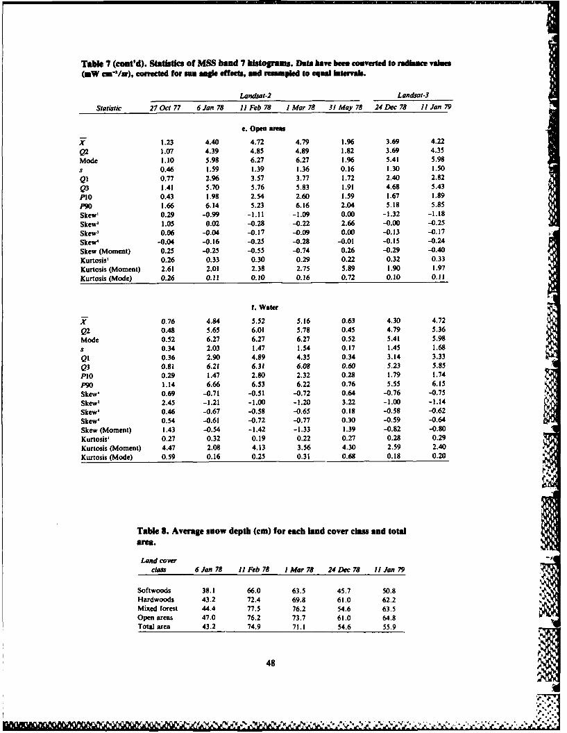
Table 7 (cont'd). Statistics of MSS band 7 histograms. Date have bean converted to radiance valem(rW cmn-/u), corrected for a anle effect, and rempled to equal intervals.

Landsat-2 Landsat-3

Statistic 27 Oct 77 6 Jan 78 11 Feb 78 1 Mar 78 31 May 78 24 Dec 78 11 Jan 79

e. Open areas

X 1.23 4.40 4.72 4.79 1.96 3.69 4.22

Q2 1.07 4.39 4.85 4.89 1.82 3.69 4.35

Mode 1.10 5.98 6.27 6.27 1.96 5.41 5.98

s 0.46 1.59 1.39 1.36 0.16 1.30 1.50

QI 0.77 2.96 3.57 3.77 1.72 2.40 2.82Q3 1.41 5.70 5.76 5.83 1.91 4.68 5.43

PlO 0.43 1.98 2.54 2.60 1.59 1.67 1.89P90 1.66 6.14 5.23 6.16 2.04 5.18 5.85Skew' 0.29 -0.99 -1.11 -1.09 0.00 -1.32 -1.18Skew' 1.05 0.02 -0.28 -0.22 2.66 -0.00 -0.25Skew' 0.06 -0.04 -0.17 -0.09 0.00 -0.13 -0.17

Skew4 -0.04 -0.16 -0.25 -0.28 -0.01 -0.15 -0.24

Skew (Moment) 0.25 -0.25 -0.55 -0.74 0.26 -0.29 -0.40

Kurtosis' 0.26 0.33 0.30 0.29 0.22 0.32 0.33Kurtosis (Moment) 2.61 2.01 2.38 2.75 5.89 1.90 1.97

Kurtosis (Mode) 0.26 0.11 0.10 0.16 0.72 0.10 0.11

f. Water

X 0.76 4.84 5.52 5.16 0.63 4.30 4.72

Q2 0.48 5.65 6.01 5.78 0.45 4.79 5.36

Mode 0.52 6.27 6.27 6.27 0.52 5.41 5.98

s 0.34 2.03 1.47 1.54 0.17 1.45 1.68

QI 0.36 2.90 4.89 4.35 0.34 3.14 3.33Q3 0.81 6.21 6.31 6.08 0.60 5.23 5.85P10 0.29 1.47 2.80 2.32 0.28 1.79 1.74

P90 1.14 6.66 6.53 6.22 0.76 5.55 6.15Skew' 0.69 -0.71 -0.51 -0.72 0.64 -0.76 -0.75

Skew' 2.45 -1.21 -1.00 -1.20 3.22 -1.00 -1.14

Skew' 0.46 -0.67 -0.58 -0.65 0.18 -0.58 -0.62Skew' 0.54 -0.61 -0.72 -0.77 0.30 -0.59 -0.64

Skew (Moment) 1.43 -0.54 -1.42 -1.33 1.39 -0.82 -0.80

Kurtosis' 0.27 0.32 0.19 0.22 0.27 0.28 0.29Kurtosis (Moment) 4.47 2.08 4.13 3.56 4.30 2.59 2.40

Kurtosis (Mode) 0.59 0.16 0.25 0.31 0.68 0.18 0.20

Table 8. Average snow depth (cm) for each land cover class and total

Land cover -j

class 6 Jan 78 11 Feb 78 1 Mar 78 24 Dec 78 11 Jan 79

Softwoods 38.1 66.0 63.5 45.7 50.8Hardwoods 43.2 72.4 69.8 61.0 62.2Mixed forest 44.4 77.5 76.2 54.6 63.5Open areas 47.0 76.2 73.7 61.0 64.8Total area 43.2 74.9 71.1 54.6 55.9

48

pb

levels. For the total area histograms the means and kurtosis. The trends in the skewness and kur-vary by less than 0.05 mW cm-2 sr-' for the three tosis are less useful for open areas than for waterLandsat-2 scenes and by 0.44 for all snow days areas because of the strong divergence from a(Fig. 24). Changes in skewness and kurtosis are ir- Gaussian distribution for the open areas.regular and do not relate well with increasing snow Although the differences between the snowdepth. scenes are variable in their suggestion of a snow

In MSS 5 the measures of central tendency and depth/regional histogram relationship, this is notpercentiles are often within 0.064 mW cm-2/sr be- the case for comparing the snow scenes, con-tween days, particularly when those of one satel- sidered as a group, with the non-snow scenes. Thelite's observations are considered. Where differ- most striking differences occur for the water sur-ences are greater than 0.064, most commonly they faces in MSS 5 and 7. Increases of greater thanshow decreases in magnitude for the days with 500% are found for all measures of central tend-greater snow depth. Th greater contribution of ency, quartiles, and percentiles. The water histo-snow to the observed Landsat signal is not occur- grams under non-snow conditions display low ra-ring with increasing snow depth because of the diance values with a tight cluster around the meandominance of the forest canopy within the (Fig. 27). Subsequent freezing and covering bysensor's instantaneous field of view. snow increases the histogram mode to higher en-

Within the nonforested cover classes, the cor- ergy values with a larger standard deviation. Thisrected histograms show a relationship between in- is described by the change in magnitude of thecreasing snow depth and the magnitude of reflect- mean, median, etc., the large increase in standarded energy. As the snow accumulates throughout deviation, the reversal of skewness from positivethe snow season, the means and in particular the to negative, and the decreased value of the mo-first quartile and 10th percentile increase in mag- ment coefficient of kurtosis.nitude. The moment coefficients of skewness and Open areas are affected similarly to water by thekurtosis for the open areas and frozen water sur- addition of snow cover. The snow depths in allfaces also show a consistent change in histogram snow scenes are greater than 38 cm. Most low-shape as the snow depth increases. Snow depth lying vegetation is covered, providing a largely un-measurements were not made over the water sur- disturbed, highly reflective snowpack. The per-faces, but the lakes and rivers remained frozen centage changes in MSS 7 are not as great as forthroughout the winter season. Even with differ- water for two reasons: 1) irregularities in the vege-ences in accumulation caused by drifting, it may tation canopy and possible anthropogenic struc-be assumed that as regional snow depth increased, tures in the agriculture areas contribute sections ofthe accumulation on the frozen water surfaces also lower reflectance, and 2) the non-snow reflectanceincreased, of the open lands is higher than that of water. This

In MSS 7, the water surfaces show consistent in- is particularly true for the May scene when vegeta-creases in magnitude (within each Landsat group) tion growth results in a higher near-infrared re-for the mean and particularly the first quartile and flectance. Water absorbs radiation in the near-in-10th percentile. These indicate a reduction in the frared wavelengths. Percentage changes for thelow reflecting portions of the histogram. This is measures in MSS 5 are similar to those for water.also shown in moment coefficients of skewness The absolute dimension of the snow values is notand kurtosis, both of which are dimensionless in- as high as for water in winter. Again, this is be-dices of data distribution. Thus, they allow for cause of the presence of darker surfaces of dor-comparison between the two Landsat passes. The mant vegetation.moment coefficient of skewness is negative be- For forested sites, the contrast between snowcause of the high mean values and the departure and no-snow scenes will depend on species compo-from symmetry to the left. It increases with snow sition, season of the no-snow scene, and banddepth largely because of the increasing value of wavelength. The softwood trees retain their leavesthe mean. The moment coefficient of kurtosis will throughout the winter and display a high crownincrease as a distribution becomes more peaked. A closure. In MSS 5, the histograms are almost iden-normal distribution will have a kurtosis (moment) tical for the October and May scenes. Increases ofof 3. Thus, the water histograms show increasing close to 100% are shown in these forests with thekurtosis with snow depth. addition of snow. Radiance changes in MSS 7 are

For open areas, the histograms again show in less pronounced, although they still occur. This isboth bands an increase in magnitude, skewness, largely because of the infrared reflectance of the

49 e

conifer leaf structure, which remains the same Table 9. Areal dtemintlon ofthroughout the autumn and winter, wow depth and water equivalet

The results of snow cove- ", the hardwoods and for the baia.mixed forest are similar to tie softwoods. In allseasons, the hardwoods display energy values sev- L.mdA Snow depth equi lnteral levels higher than do the evergreens in both date (Cn) (Cn)MSS 5 and 7. Canopy structure and the loss ofleaves in the winter are responsible for this in- 6 Jan 78 42.27 7.42creased reflectance. Percentage changes between 11 Feb 78 73.58 20.24no-snow and snow scenes are comparable for all I Mar 78 70.94 19.46

forest types. The one exception occurs when the 24 Doc 78 51.92 6.10

May scene and the winter scenes for MSS 7 are

compared. In northern Maine, the hardwoods leafout in late May. The leaf cellular structure andgeometry result in high infrared reflectance. Themagnitude of the energy in MSS 7 during May is through 31 May 1978 was used for the simulationequal to and often exceeds that for the snow- model run. Calibration of the Upper Saint Johncovered scene. River Basin was accomplished by the New Bruns-

The forests display a smaller change between wick Flood Forecast Centre. The parameters ofnon-snow and snow conditions than either open soil moisture index and rain-freeze temperatureareas or water. However, there is still a measure- were adjusted to optimize the prediction of run-able, predictable displacement by several histo- off. The results of the SSARR run are shown ingram levels for most statistical measures. Figure 28.

If Landsat bands 5 and 7 are considered to- The initial SSARR run showed that the magni-gether, the Landsat histograms-corrected to ac- tude of the first predicted runoff peak comparedcount for the solar angle and sensor calibration- to the observed values for the Ninemile Bridge,could provide an automated evaluation of the Dickey, and Allagash subbasins was 58%, 70%,presence and areal distribution of a snowpack, and 78%, respectively. The magnitude of the sec-even in a heavily forested region such as northern ond predicted runoff peak for the Dickey and Al-New England. The MSS 7 statistics for the 27 Oct lagash subbasins was 97% and 70%, respectively,scene are significantly different from the other of the recorded stream discharge values, whereasscenes (Table 7). Because of leaf emergence, the 31 the second runoff peak for the Ninemile BridgeMay MSS 7 histogram statistics are similar to the subbasin was overpredicted by 3%.snow scenes, although this similarity does not ap- The time of the first predicted peak of runoffpear in MSS band 5. was earlier bb 8 days for the Ninemile Bridge and

Allagash subbasins and by 9 days for the DickeyLandsat data as input subbasin. The timing of the second predicted peakto the SSARR model improved for Ninemile Bridge, Dickey, and Alla-

The 31 May Landsat land cover classification gash, with a delay of 2, 3, and 5 days, respectively.provided a basis upon which the point measure- In summary, the initial baseflow period (1-27ments of water equivalent could be used in the March) predicted by the SSARR model was withinSSARR model. The snow course measurements 78% of the recorded stream discharge values. Thewere selected to provide data for the various land spring melt recession (10-31 May 1978) predictedcover classes present in the entire hydrologic by the SSARR model was within 67% of the re-basin. The ground measurements of water equiva- corded stream discharge values. The timing of thelent of snow were subsequently area-weighted to six runoff peaks (Fig. 28) lagged by 2 to 9 days.the May Landsat classification to derive mean The magnitude of the six predicted runoff peaksregional water equivalent estimates for each of the was within 75% of the recorded streamflow meas-five Landsat winter scenes (Table 9). urements. The error in the prediction of the initial

The I Mar 78 estimate of 19.46 cm of water storm peak for all three subbasins was attributedequivalent was used as an input value to the to the underprediction of snowmelt by the SSARRSSARR model. This value was an estimate of model caused by a rain-on-snow event that oc-snow water equivalent before the spring melt peri- curred on 28 March.od had occurred. The time period of 1 March

S50

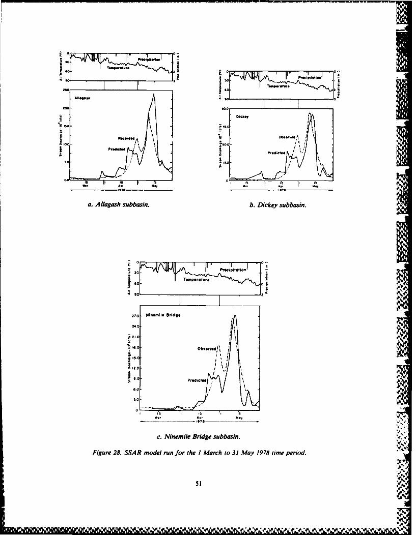
9o 3. so I

2112

Wit -600

~Dickey

S- R~~~fcorded4 bew~~

Predicted ,

re

L Predicted

SI 0.0 0, 1...".0

I's -i s I' r-3s I "

6 Go-2

0240

U., Am Ie o up o

1971 19711

a. Allagah subbain. b. Dickey subbazsin.

.--

'30. Pr i ,,.,,..cI -ed

6 0 f

4 9 0 1 ' 3 .t 0

270 Ninmil n ridle Bi24 0 i

"<I_. .o . ii

1.0

I 15

51'.

6.0iemleBrdg subsn ".

Figure 28~.0A oe u o h ac o3 a 98tm eid

0N

In temperate continental climatic zones, addi- years' time, the Landsat data can be used periodi-tional complications in spring melt arise when cally to develop a current land cover inventory ofrain-on-snow events occur. The rainfall coupled the basin.with above-freezing temperatures can cause thesnowpack to melt very rapidly. This type of occur-rence may have to be modeled as a separate sub- LITERATURE CITEDroutine with SSARR. Additional work on recali-brating the basin peak timing and melt rate factors Adams, W.P. (1976) Areal differentiation of snowis also required. cover in east central Ontario. Water Resources Re-

search, 12(6): 1226-1234.Adams, W.P. and D.R. Barr (1979) Vegetation-

CONCLUSIONS snow relationships in Labrador. In Proceedings ofthe 36th Annual Meeting of the Eastern Snow

Initial histogram analysis presented in this study Conference. Alexandria Bay, New York, pp. 1-indicated that a good correlation existed between 25.the satellite radiometric measurements and mean Adams, W.P. and N.T. Roulet (1982) Areal dif-snow depth in the 420-km2 area. Using Landsat un- ferentiation of land and lake snowcover in a smallcorrected data an equation was developed to pre- subarctic drainage basin. Nordic Hydrology, 13:dict snow depth with a standard error of estimate 139-156.of ±5 cm. Alfoidi, T.T. (1976) Digital analysis of Landsat

However, when subsequent corrections for sen- MSS imagery for snow mapping applications.sor calibrations and solar elevation were taken in- Canada Centre for Remote Sensing, Energy,to consideration, this correlation was eliminated Mines and Resources, Technical Report, 21 pp.for forested land cover. For open clearings and Anderson, D.M., H.L. McKlm, L.W. Gatto,frozen water surfaces, definite increases in histo- R.K. Haugen, W.K. Crowder, C.W. Slaughtergram means, quartiles, percentiles, kurtosis, and and T.L. Marlar (1974) Arctic and subarctic envi-skewness were observed as regional snow depth in- ronmental analyses utilizing ERTS-l imagery.creased. Some of our correlations would compare Type III Final Report to NASA for the periodbetter with western snowpack satellite relation- June 1972-February 1974, Contract No.ships if the models for western snowpacks had to S-70253-AG, 112 pp.contend with freeze-thaw cycles and rain-on-snow Anderson, H.W. (1969) Storage and delivery ofevents. These two factors will definitely change rainfall and snowmelt water as related to forestthe reflectance and brightness characteristics of environments. In Proceedings of the Third Forestthe snowpack. Microclimate Symposium, Canadian Forestry Ser-

The ground measurements of water equivalent vice (J.M. Powell and C.F. Nolasco, Ed.), Cal-were area-weighted by the May land cover classifi- gary, Alberta, pp. 51-67.cation to derive a mean regional water equivalent Anderson, H.W. and T.H. Pagenhart (1957)estimate for input to the SSARR model. For the Snow on forest slopes. In Proceedings of the 25thtime period of 1 March through 31 May 1978, the Annual Meeting Western Snow Conference, SantaSSARR model prediction was within 78% of the Barbara, California, 17-19 April, pp. 19-23.measured runoff for the initial baseflow period Barnes, J.C. and C.J. Rowley (1973) Use of ERTSand within 67% for the spring melt recession peri- data for mapping snow cover in the the westernod. The timing and magnitude of the runoff peaks United States. Symposium on Significant Resultsrequires additional work on recalibrating the basin from ERTS-I, 5-9 March, New Carrollton, Mary-peak timing factors and melt rate factors. land, pp. 855-862.

A technique was developed for using minimal Barnes, J.C. and C.J. Bowley (1974) Handbookground truth snow course measurements coupled of techniques for satellite snow mapping. Con-with a Landsat land cover classification to derive a cord, Massachusetts: Environmental Researchmean areal average of water equivalent. This tech- and Technology, Inc., Document No. 0407-F, 95nique could be demonstrated for other watersheds pp.by selecting an appropriate number of snow cours- Barnes, J.C. and M.D. Smallwood (1975) Synop-es representative of land cover types. In forested sis of current satellite snow mapping techniques,basins where land cover can change within a few with emphasis on the application of near-infrared

52

data. Operational Applications of Satellite Snow- Daflam, W.C. and J. Foster (1975) Digital snowcover Observations, Workshop held at South Lake mapping technique using Landsat data and Gener-Tahoe, California, 18-20 August, NASA SP-391, al Electric IMAGE 100 system. Operational Ap-pp. 199-213. plications of Satellite Snowcover Observations,furry, R.G. (1983) Research on snow and ice. Re- Workshop held at South Lake Tahoe, California,views of Geophysics and Space Physics, 21(3): 18-20 August. NASA SP-391, pp. 259-278.765-776. Dey, B., D.C. Goswami and A. Rango (1983)Bartolacc, L.A., R.M. Hoffer and S.G. Luther Utilization of satellite snow-cover observations(1975) Snowcover mapping by machine processing for seasonal streamflow estimates in the Westernof Skylab and Landsat data. OperationalApplica- Himalayas. Nordic Hydrology, pp. 257-266.tions of Satellite Snowcover Observations, Work- Dirmhirn, 1. and F.D. Eaton (1975) Some charac-shop held at South Lake Tahoe, California, 18-20 teristics of the albedo of snow. Journal of AppliedAugust, NASA SP-391, pp. 295-311. Meteorology, 14(3): 375-379.Dates, R. (1983) Snow cover and meteorology at Dozier, J., S.R. Schneider and D.F. McGinnis, Jr.Allagash, Maine, 1977-1980. USA Cold Regions (1981) Effect of grain size and snowpack waterResearch and Engineering Laboratory, Special equivalence on visible and near-infrared satelliteReport 83-20, 53 pp. observations of snow. Water Resources Research,Bauer, K.G. and J.A. Dutton (1962) Albedo vari- 17(4): 1213-1221.ations measured from an airplane over several Draeger, W.C. and D.T. Lauer (1974) Areal ex-types of surface. Journal of Geophysical Re- tent of snow in forested regions, a practical esti-search, 67(6): 2367-2376. mation technique using ERTS-I data. In Proceed-Bergen, J.D. (1975) A possible relation of albedo ings of the 9th Symposium on Remote Sensing ofto the density and grainsize of natural snow cover. Environment, Ann Arbor, Michigan, 15-19 April,Water Resources Research, 11(5): 745-746. vol. 1, pp. 333-339.Blyth, K., M.A.R. Cooper, N.E. Lindsey and Dunkle, R.V. and J.T. Bevans (1956) An approxi-R.B. Painter (1974) Snow depth measurements mate analysis of the solar reflectance and trans- .with terrestrial photos. Photogrammetric Engi- mittance of a snow cover. Journal of Meteorol-neering, 40(8): 937-942. ogy, 13: 212-216.Bohren, C.F. and R.L. Beschta (1979) Snowpack Dutton, J.A. (1962) An addition to the paper 'Al-albedo and snow density. Cold Regions Science bedo variations measured from an airplane overand Technology, 1(1): 47-50. several types of surface.' Journal of GeophysicalBowley, C.J., J.C. Barnes and A. Rango (1981) Research, 67(13): 5365-5366.Satellite snow mapping and runoff prediction Environmental Research and Technology, Inc.handbook. Applications Systems Verification and (1977) Terrestrial ecosystem analysis, Dickey-Transfer Project, vol. III. NASA Technical Paper Lincoln School Lakes Project, Maine, Document1829, 87 pp. P-2037 prepared for the U.S. Army Corps of En- SBIdyko, M.I. (1974) Climate and Life (Translated gineers, New England Division, 236 pp.by D.H. Miller). New York: Academic Press, In- Federer, C.A. (1971) Radiation absorption byternational Geophysical Series, vol. 18. leafless hardwood forests. Agricultural Meteorol-Castruccio, P., H. Loats, D. Lloyd and P. New- ogy, 9: 3-20.man (1981) Cost/benefit analysis for the ASVT on Ferguson, H.L. and S. Lapczak (1977a) Analysisoperational applications of satellite snow-cover of snow cover over the Saint John and Sourisobservations. Applications Systems Verification River Basins. Progress Report for WMO Snowand Transfer Project, vol. III. NASA Technical Studies by Satellite Project. Downsview, Ontario: . .Paper 1828, 240 pp. Atmospheric Environment Service.Chondbry, B. (1982) Spectral a!bedos of mid-lat- Ferguson, H.L. and S. Lapczak (1977b) Satelliteitude snowoacks. Cold Regirns Science and Tech- imagery analysis of snow cover in the Saint Johnnology, 6(2): i23-139. and Souris River basins. In Proceedings of the 4thCooper, S., P. Bock, J. Horowitz and D. Foran Canadian Symposium on Remote Sensing, Que-(1975) The use of ERTS imagery in reservoir man- bec, 16-18 May. Ottawa, Ontario: Canadian Aer-agement and operation. Final Report for NASA, onautics and Space Institute, pp. 126-142.105 pp.

53

FitaGibbon, J.E. and T. Dune (1979) Character- ning Multichannel Microwave Radiometeristics of subarctic snowcover. Hydrological Sci- (SMMR) data. IEEE Transactions on Geoscienceences Bulletin, 24(4): 465-476. and Remote Sensing, GE201(4): 452-467.Giddings, J.C. and E. La Chapelle (1961) Diffu- Kurilova, Yu.V. (1975) Investigations of the snowsion theory applied to radiant energy distribution cover from satellite data. Institute of Water Prob-and albedo of snow. Journal of Geophysical Re- lems, Academy of Sciences of the USSR (trans-search, 66(1): 181-189. lated from Vodnye Resursy), 2: 50-60.Golding, D.L. (1974) Snow cover and melting Kwilova, Yu.V., P.A. Kolosov, L.K. Poplav-snow from ERTS imagery. Canadian Surveyor, skaya and Yu.S. Sokolov (1976) Investigation of29(2):128-134. the dynamics of snow-cover melting from meteor-Granberg, H.B. (1972) Snow depth variations in a ological-satellite data. Transactions of the Stateforest-tundra environment, Schefferville, P.Q. Hydrologic Institute (Trudy GGI), 237: 22-31.Winter 1968-1969. M.Sc. Thesis (unpub.), McGill Also in Soviet Hydrology: Selected papers, 15(21).University, 134 pp. Langham, E.J. and J.M. Power (1977) RemoteGranberg, H.B. (1975) Snow in different rough- sensing of snow by satellite. In Proceedings of theness zones at Schefferville: its character and hy- 2nd Conference on Hydrometeorology, Toronto,drologic significance. In Proceedings of the 32nd Ontario, Canada, 25-27 October. Boston: Ameri-Eastern Snow Conference, pp. 108-123. can Meteorological Society, pp. 268-271.Hansen, P.L. (1975) Experiences in snow cover Leonard, R.E. and A.R. Eschner (1968) Albedomapping in the Saint John River Basin. In Pro- of intercepted snow. Water Resources Research,ceedings of the 3rd Canadian Symposium on Re- 4(25): 931-935.mote Sensing, Edmonton, Alberta, 22-24 Septem- IAchtenegger, J., K. Seidel, M. Keller and H.ber (G.E. Thompson, Ed.). Ottawa, Ontario: Haefner (1981) Snow surface measurements fromCanadian Aeronautics and Space Institute, pp. digital Landsat MSS data. Nordic Hydrology, 12:315-322. 275-288.Itten, K.I. (1975) Approaches to digital snow Lillesand, T.M., D.E. Meisner, A.L. Downs andmapping with Landsat-1 data. Operational Appli- R.L. Deueil (1982) Use of GOES and TIROS/cations of Satellite Snowcover Observations, NOAA satellite data for snow-cover mapping.Workshop held at South Lake Tahoe, California, Photogrammetric Engineering and Remote Sens-18-20 August, NASA SP-391, pp. 235-247. ing, 48(2): 251-259.Katibah, E.F. (1975a) Areal extent of snow esti- Luther, S.G., L.A. Bartolucci and R.M. Hoffermation in the northern Sierra Nevada mountains (1975) Snow cover monitoring by machine proc-using Landsat-I imagery. In Proceedings of the essing of multitemporal Landsat MSS data. Oper-NASA Earth Resources Survey Symposium, Hous- ational Applications of Satellite Snowcover Ob-ton, Texas, June. NASA TM X-58168, pp. servations, Workshop held at South Lake Tahoe,2621-2641. California, 18-20 August. NASA SP-391, pp.Katibab, E.F. (1975b) Operational use of Landsat 279-311.imagery for the estimation of snow areal extent. Martinec, J. (1975) Snowmelt-runoff model forOperational Applications of Satellite Snowcover stream flow forecasts. Nordic Hydrology, 6: 145-Observations, Workshop held at South Lake 154.Tahoe, Caifornia, 18-20 August, NASA SP-391, Martinec, J. (1982) Runoff modeling from snow-pp. 129-142. covered area. IEEE Transactions on GeoscienceKondratyev, K.Ya. (1969) Radiation in the Atmo- and Remote Sensing, GE-20(3): 259-262.sphere. International Geophysical Series, vol. 12. Martinec, J. and A. Rango (1981) Areal distribu-New York: Academic Press. tion of snow water equivalent evaluated by snowKung, E.C., R.A. Bryson and D.H. Lenschow cover monitoring. Water Resources Research,(1964) Study of a continental surface albedo on 17(5): 1480-1488.the basis of flight measurements and structure of Martimec, J., A. Rango and E. Major (1983) Thethe Earth's surface cover over North America. snowmelt-runoff model (SRM) user's manual.Monthly Weather Review, 92(2): 543-564. NASA Ref. Pub. 1100. Greenbelt, Maryland:Kunzi, K.F., S. Patti and H. Rott (1982) Snow- NASA Goddard Space Flight Center, 118 pp.cover parameters retrieved from Nimbus-7 Scan-

54

MatheIr, TJ. (1980) The role of vegetation on the Meier, M.F. (1973) Evaluation of ERTS imagerydisposition of snowfall on a mixed forested water- for mapping and detection of changes of snow-shed in the Kawatha Lakes region of east central cover on land and on glaciers. Symposium on Sig-Ontario. Studies in Snow and Ice (N.T. Roulet, nificant Results Obtained from ERTS-i, NewEd.). Trent Student Geographer, vol. 8. Peterbor- Carrollton, Maryland, 5-9 March, pp. 863-875.ough, Ontario: Trent University, pp. 36-50. Meier, M.F. (1974) New ways to monitor the massMatson, M. and D.R. Wlesnet (1981) New data and areal extent of snowcover. COSPAR, Ap-base for climate studies. Nature, 289(5797): 451- proaches to Earth Survey Problems through use of456. Space Techniques, F.R.G., 23-25 May 1973. Ber-McFadden, J.D. and R.A. Ragotzkle (1967) Cli- lin: Akademie-Verlag, pp. 241-250.matological significance of albedo in central Meier, M.F. (1975a) Application of remote-sens-Canada. Journal of Geophysical Research, 72(4): ing techriques to the study of seasonal snow1135-1143. cover. Journal of Glaciology, 15(73): 251-265.McGinnis, D.F., Jr. (1975) A progress report on Meier, M.F. (1975b) Satellite measurement ofestimating snow depth using VHRR data from snowcover for runoff prediction. Presented at I I thNOAA environmental satellites. Operational Ap- American Water Resources Conference, Batonplications of Satellite Snowcover Observations, Rouge, Louisiana, 24 pp.Workshop held at South Lake Tahoe, California, Meier, M.F. and W.E. Evans (1975) Comparison18-20 August, NASA SP-391, pp. 313-324. of different methods for estimating snowcover inMcGinnis, D.F., Jr., J.A. Pritchard and D. Wies- forested, mountainous basins using Landsatnet (1975) Determination of snow depth and snow (ERTS) images. Operational Applications of Sat-extent from NOAA-2 satellite Very High Resolu- ellite Snowcover Observations, Workshop held attion Radiometer data. Water Resources Research, South Lake Tahoe, California, 18-20 August,11(6): 897-902. NASA SP-391, pp. 215-234. ,McGinnis, D.F., Jr., R.A. Scofleld, S.R. Schneid- Metman, J.R. (1970) Snow accumulation relateder and C.P. Berg (1979) Satellites as an aid to to elevation, aspect and forest canopy. In Pro-water resource managers. ASCE Convention, Bos- ceedings of the Workshop Seminar on Snow Hy-ton, Massachusetts, 2-6 April. drology. Queen's Printer, pp. 35-47.McKim, H.L. (1975) Vegetation analysis of the Mellor, M. (1965) Optical measurements on snow.Dickey-Lincoln area, Maine. Map overlays pro- USA Cold Regions Research and Engineeringvided to the New England Divisian, Corps of En- Laboratory, Research Report 169, 19 pp.gineers, showing vegetation types. Mellor, M. (1977) Engineering properties of snow.MeKim, H.L. and C.J. Merry (1975) Use of re- Journal of Glaciology, 19(81): 15-66.mote sensing to quantify construction material Merry, CJ. and H.L. McKim (1978) Computerand to define geologic lineations-Dickey-Lin- processing of Landsat digital data and sensor in-coin School Lakes Project, Maine. USA Cold Re- terface development for use in New England reser-,.,Igions Research and Engineering Laboratory, Spe- voir management. USA Cold Regions Research ..,cial Report 242, parts I and 2, 26 pp. and Engineering Laboratory, Special Report 78-6.McMillan, M.C. and D.F. McGinnis (1975) The 66 pp.possibility of determining snowpack surface con- Merry, C.J., H.L. McKim, S. Cooper and S.G.ditions using remote multispectral techniques. In Ungar (1977) Preliminary analysis of water equiv-Workshop for Environmental Applications of alent/snow characteristics using Landsat digital .Multispectral Imagery, Ft. Belvoir, Virginia, 11- processing techniques. In Proceedings of the East-13 November. U.S. Army Engineer Topographic ern Snow Conference, Belleville, Ontario, 3-4 Feb-Laboratories and American Society of Photogram- ruary, pp. 39-54. -r

metry, pp. 304-313. NASA (1982) Plan of research for snowpackMcMillan, M.C. and J.L. Smith (1975) Remote properties remote sensing-(PRS), Recommen-sensing of snowpack density using shortwave radi- dations of the snowpack properties workingation. Operational Applications of Satellite Snow- group. Greenbelt, Maryland: NASA Goddardcover Observations, Workshop held at South Lake Space Flight Center, 38 pp.Tahoe, California, 18-20 August, NASA SP-391, New England Division, Corps of Engineers (1967)pp. 361-373. Saint John River Basin, Dickey-Lincoln School

Project, Maine, U.S.A., and Quebec, Canada.

55 %

-7

Department of the Army, New England Division, RangO, A. (1981) Application systems verificationCorps of Engineers: Waltham, Massachusetts, and transfer project. Vol. I. Operational applica-Design Memorandum No. 4. tions of satellite snow cover observations-execu-Nicholson, F.H. (1975) Snow depth mapping tive summary. NASA Technical Paper 1822, 81from aerial photographs for use in permafrost pp.predictions. In Proceedings of the 32nd Eastern RangO, A. (1983) Application of a simple snow-Snow Conference, pp. 124-136. melt-runoff model to large river basins. In Pro-O'lrien, H.W. and G. Kok (1981) Near-infrared ceedings of the 1983 Western Snow Conference,reflectance of snow-covered substrates. USA Cold pp. 89-99.Regions Research and Engineering Laboratory, Rango, A. and K.I. Itten (1976) Satellite poten-CRREL Report 81-21. tials in snow cover monitoring and runoff predic-O'Brien, H.W. and R.H. Mouns (1975) Red and tion. Nordic Hydrology, 7: 209-230.near-infrared spectral reflectance of snow. USA Range, A. and J. Martinec (1979) Application ofCold Regions Research and Engineering Labora- a snowmelt-runoff model using Landsat data.tory, Research Report 332. Nordic Hydrology, 10(4): 225-238.O'Neill, A.D.J. and D.M. Gray (1973) Solar radi- Rango, A. and J. Martinec (1981) Accuracy ofation penetration through snow. In The Role of snowmelt runoff simulation. Nordic Hydrology,Snow and Ice in Hydrology, Proceedings of the 12: 265-274. -Banff Symposia, September 1972. Published Rango, A. and J. Martinec (1982) Snow accumu-jointly by WMO (Geneva), IAHS (Budapest), and lation derived from modified depletion curves ofUNESCO (Paris), pp. 227-241. snow coverage. In HydrologicalAspects of AlpineParry, J.T. and B.J. Grey (1975) The mapping and High-Mountain Areas, Proceedings of the Ex-and interpretation of snow conditions in Quebec- eter Symposium (J.W. Glen, Ed.). IAHS Publ.Labrador using ESSA-9 composite minimum no. 138, pp. 83-90.brightness (CMB) charts. Photogrammetria, 30(2): Rango, A. and V.V. Salomonson (1976) Satellite41-66. snow observations and seasonal streamflow fore-Patch, J.R. (1981) Effects of forest cover on snow casts. Final Report under NOAA Contract No.cover distribution in the Nashwaak Experimental NA-776-74, 19 pp.Watershed Project. In Proceedings of the 38th Rango, A., J.F. Hannaford, R.L. Hall, M. Ro-Annual Eastern Snow Conference, 4-5 June, Syr- senzweig and A.J. Brown (1979) Snow-coveredacuse, New York, pp. 76-87. area utilization in runoff forecasts. Journal of thePower, J.M., CJ. Merry, N.B.A. Trivett and Hydraulics Division, Proceedings of the AmericanS.E. Waterman (1980) Snowpack estimation in the Society of Civil Engineers. Proc. Paper 14326,St. John River Basin. In Proceedings of the 14th 105(HYI): 53-66.International Symposium on Remote Sensing of Rango, A., V.V. Salomonson and J.L. FosterEnvironment, San Jose, Costa Rica, 23-30 April, (1975) Operational water management applica-pp. 467-486. tions of snowcovered area observations. In Pro-Rango, A. (1975) Operational applications of sat- ceedings of the NASA ERTS Symposium, Hous-ellite snowcover observations project. in Proceed- ton, Texas, June. NASA TM X-58168, pp. 2669-ings of the l0th International Symposium on Re- 2685.mote Sensing of Environment, 6-10 October, Ann Rasmumen, W.O. and P.F. Ffolliott (1979) Pre-Arbor, Michigan. Ann Arbor: Environmental Re- diction of water yield using satellite imagery and asearch Institute of Michigan, pp. 1367-1376. snowmelt simulation model. Unpublished report.Rato, A. (1978) Pilot tests of satellite snow- Seldel, K., F. Ade and J. Lichtenegger (1983)cover/runoff forecasting systems. NASA Techni- Augmenting Landsat MSS data with topographiccal Memorandum 78109, 13 pp. information for enhanced registration and classifi-Rango, A. (1980a) Remote sensing of snow-coy- cation. IEEE Transactions on Geoscience and Re-ered area for runoff modelling. In Hydrological mote Sensing, GE-21(3): 252-258.Forecasting, Proceedings of the Oxford Sympos- Shafer, B.A., C.F. Leaf, J.A. Danielson and G.F.ium, April. IAHS Publ. no. 129, pp. 291-297. Moravec (1981) Operational applications ofRango, A. (1980b) Operational applications of satellite snow-cover observations-Colorado Fieldsatellite snow cover observations. Water Re- Test Center. Applications Systems Verificationsources Bulletin, 16(6): 1066-1073. and Transfer Project, vol. IV. NASA Technical

Paper 1825, 101 pp.

56

mom

--n

Sarep, J.M. (1975) A comparison of operational Thomas, V.L. (1975) Generation and physicaland Landsat-aided snow water content estimation characteristics of the Landsat-I and -2 MSS com-systems. Operational Applications of Satellite puter compatible tapes. NASA document X563-Snowcover Observations, Workshop held at South 75-223. Greenbelt, Maryland: NASA GoddardLake Tahoe, California, 18-20 August. NASA SP- Space Flight Center, 73 pp.391, pp. 325-344. Thompson, A.G. (1975) Utilization of LandsatSharp, J.M. and R.W. Thomas (1975) A cost- monitoring capabilities for snowcover depletioneffectiveness comparison of existing and Landsat- analysis. Operational Applications of Satelliteaided snow water content estimation systems. In Snowcover Observations, Workshop heldat SouthProceedings of the 10th International Symposium Lake Tahoe, California, 18-21 August. NASAon Remote Sensing of Environment, 6-10 Octo- SP-391, pp. 113-127.ber, Ann Arbor, Michigan. Ann Arbor: Environ- Thomsen, A.G. and W.D. Striffler (1980) Spatialmental Research Institute of Michigan, pp. 1255- simulation of snow processes. Symposium on1262. Watershed Management, Boise, Idaho, 21-23 Ju- UShunying, Z., Z. Qunzhu, C. Xianzhang and J. ly. New York: American Society of Civil Engi-Dehong (1980) Studies on snow depth and snow neers, vol. 1, pp. 326-334.runoff with images from NOAA-5 satellite. Kexue Ungar, S.G. (1977) Multispectral Image AnalysisTongbao, 25(11): 942-946. Package (MAP1), Version 1.1, User's Manual.Smith, D.A. (1980) Flood forecasting in the Saint Unpublished draft report, 75 pp.John River Basin, Mathematical Modeling Activi- U.S. Army Engineer Division, North Pacific .Vties. In Modeling Activities Related to Flood (1975) Program description and user manual forDamage Reduction, Proceedings of the Technol- SSARR (Streamflow Synthesis and Reservoir Reg-ogy Transfer Workshop, Technical Workshop ulation) Model. Program 724-K5-GO010, U.S. Ar-Series No. 2, Hull, Quebec, Canada, 25-29 May my Engineer Division, North Pacific, Portland,1979. Halifax, Nova Scotia: Inland Waters Direc- Oregon.torate, Environment Canada, pp. 277-311. U.S. Geological Survey and NASA (1979) LandsatSteinhoff, H.W. and A.H. Barnes (1976) Deter- Data Users Handbook.mination of snow depth and water equivalent by Warren, S.G. (1982) Optical properties of snow.remote sensing. Completion Report Series No. 76, Reviews of Geophysics and Space Physics, 20(1):Environmental Resources Center, Colorado State 67-89.University, Fort Collins, 13 pp. Warskow, W.L., T.T. Wilson, Jr. and K. KirdarSteppuhn, H. (1976) Areal water equivalents for (1975) The application of hydrometeorologicalprairie snowcovers by centralized sampling. In data obtained by remote sensing techniques forProceedings of the 44th Annual Western Snow multipurpose reservoir operations. OperationalConference, Calgary, Alberta, 20-22 April, pp. Applications of Satellite Snowcover Observations,63-68. Workshop held at South Lake Tahoe, California,Steppuhn, H. and G.E. Dyck (1974) Estimating 18-20 August. NASA SP-391, pp. 29-37.true basin snowcover. In Advanced Concepts and Wiegman, E.J., W.E. Evans and R. HadfieldTechniques in the Study of Snow and Ice Resourc- (1975) Measuring snow cover using satellite imag-es. Washington, D.C.: National Academy of Sci- ery during 1973 and 1974 melt season: North San-ences, U.S. International Hydrological Decade, tiam, Boise, and Upper Snake Basins, Phase Ipp. 314-328. Final Report. SRI Project 4122. Menlo Park, Cal-Strong, A.E., E.P. McClan and D.F. McGinnis ifornia: Stanford Research Institute, 79 pp.(1971) Detection of thawing snow and ice packs Wiscombe, W.J. and S.G. Warren (1980) A modelthrough the combined use of visible and near- for the spectral albedo of snow. I: Pure snow.infrared measurements from Earth satellites. Journal of Atmospheric Sciences, 37(12): 2712-Monthly Weather Review, 99(11): 828-830. 2733. -'

..

57 1.0

e- e2 e. e~ %e t .-- t r . -. L*V t:e n 1%" rz'V !

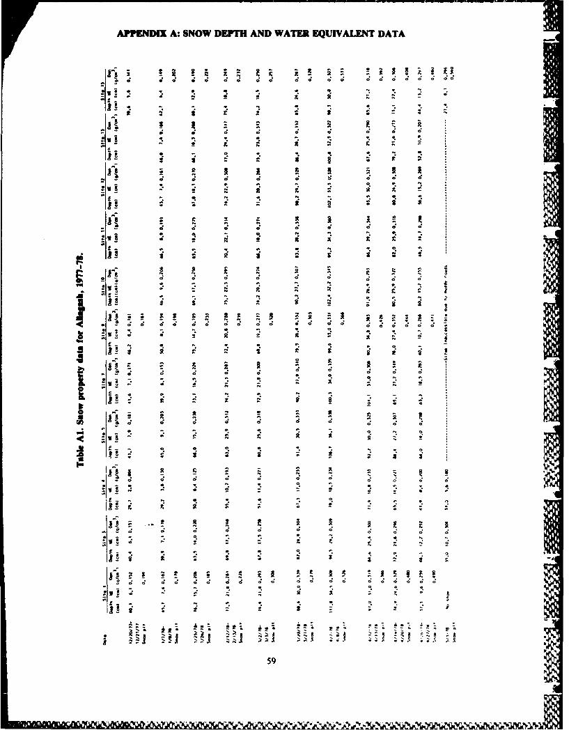
APPENDIX A: SNOW DEPTH AND WATER EQUIVALENT DATA

ja * . aa:N.................. . .

* 8 0 0 8 0 0 0 0 0 0 0 0 0 0 0 0 0 0 0 00

:12 . '. 0*

ft a a - - aas - - - F. 9

- ft ft a - a -A! *. -.a - * a a * ft

* a a a a

8 ft - N

S . .

- 0 0 0 0 0 0 0 0 0

* ft ft a 0

- - a a - ft ft -

* - 2 ft ft ft -

o ft ft S 0 ft S_ - ft ft

ft ~ 2 a

A - I - Io 0 0

- 0 0 0 0 0

* a 9 a ft a 0 9 N

:wI a a 22* ft 9 N ft - C S

* a - ft 055 a ft * - -

- a ft - 3ft ft I I

- ft a ft a F.ft - 0 0 0 0 0 0 0 0 0

* Q - 0 e ft 9:wi 2* a 2 3 F

a 9 0 *

I! a ~a ft - N N

* . 2~ x

ft 0 0 0 44o a ft a ft

a * --, ft

a ft N * * aU A! S - ; 2 2

--------------------------------- 2 ~ ±2 1 1 2 2 ~...............................-

0 0 0 0 0 0

ft a 9. o a ft ft

ft-s* ~ a 2 2 2 1

2ft ft ft ft a a a

A! s ; ~ ~U

- - 2 2 IA! -ft . . . . . 0 0 *

ft ft a a o a o * 0 e 0* ft - a a a 0 ft

a a - ft N 1 - ft a

a ft ft ft a ft ft

ft ft 0

o a - a ft -

* 18! ft a a a I

aft- ft-

N - 0

I 2 a I a - 0 0

- - ft N 0 ft N *hft* . . N N ~

o 0 0 0 0 0

* - a a * ft a ft a

4 a a o - ft a

ft a a 0

lB 2 -~ -~

a aft I I I

a . Ia ft 0 0 0 0 0 0 0 0 0 0 0

* ft ft o a a ft N- ft ft

ft a ft a

0 0 N . 0

ft S a *

I!A! ~ 2 . . .

0 0 0 0 0 0 0 0 0 0 0 0 0 0 0 0 0 0 0 0

- ft a a 0 ft 0, a a:ws - I - ft 4ft 0

N

ft

ft - N ft ft ft a a a

ft ft ft

- 2 a

- ft 0: *9 Oft

2±

5 ~ ~:aa ..- i .*.J ftft

59

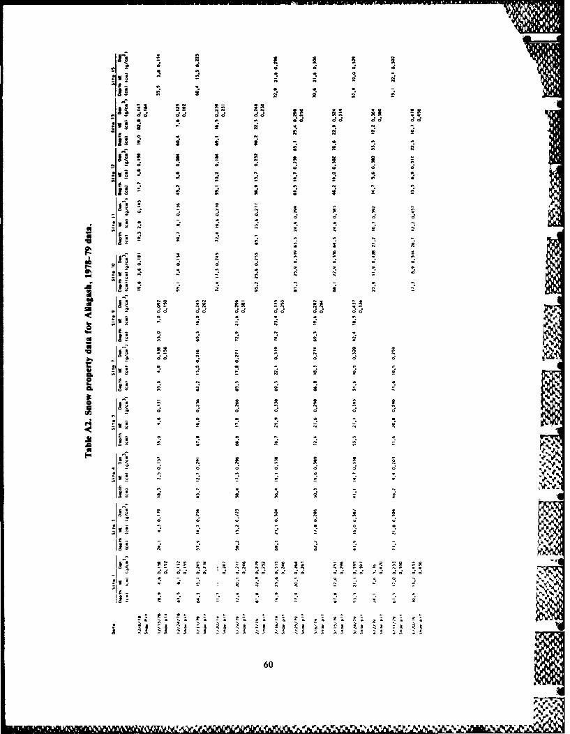
OCIOC; 4; C; C; -;oc

ms R

2 fj 1IL

a Ile-Is

it

_ C.

So 0 0N N 60

3 - aN 0 *0 N

az ga MA R;@ f! 1!

C; -

ft I n 1 I

ft It

- ~ ~ c nt* ~

2 ~~ ~ z r t f t f t f

2 c; c 0

12 - t - t 51

* a - 61

Table A4. Snow property data for Aflagash. Aditiomal data from site 1.

1977-1970 - 19711-1970 6919-195soca Oil saa pit s. pit

Dote t!P A wsII 0.iml Deta Daf Oelt I IV" Dt Df OmsI tv d-ity

12-21 40.6 1.3 0.131 -- 12-04 15.4 3.e 0.164 0.180 12-24 12.7 7.1 0.007 0.144017 .1 19 .207 0.220 12-11 15.0 2.1 0.141 0.1IU 12-31 26.4 4.6 0.161 0.140

011 41 990.105 0.197 12-16 33.1 7.1 0.129 0.138 01-14 20.3 9.6 0.473 0.24001-23 75:2 19.0 0.244 - 03.01 44.0 13.2 0.206 0. 24 01-21 22.1 1.3 0.241 0.10001,-3 1 74 4 34.1 0.191 0.205 01.05 61.5 16.3 0.297 0.231 01-29 34.6 6.0 0.190 0.1602-06 66.1 14. 01 0214 01I 71.1 19.5 0.279 0.231 02-0 34.6 6.9 0.197 0.24202-20 7s.7 21.1t 0.278 0.23S 01-22 90.9 22.4 0.244 0.212 02-16 36.3 6.4 0.1 0.23502-27 75.7 21.5 0.293 0.264 02.0 6.4 22.3 0.276 0.293 02-211 S2.1 11.4 0.219 0.24603-06 76.2 25.6 0.302 0.296 02.32 77.11 20.5 0.269 0.241 03s-045 .5 9.6 0. 16 0.74603-33s 75.0 23.9 0.306 0259 02-19 74. 23:1 0.263 0.2111 03-10 63.0 32.4 0.190 0.203-2 111.6 36.3 0.3 0.2117 Os-0 70. 24. 0.1 .1 31 1 1. .43 0261

04-03 111.0 36.1 0.321 0.1512 03-12 67.5 17.5 0. 262 0.274 03-24 69.1 14.7 0.213 0.264

03-39 66.0 14.0 0.212 0.316 03,31 27.9 6.9 0.241 0.40603-26 31.6 14.7 0.444 0.44004-03 13.5134.0 0.262 0.21604-16 13.6 19.5 0.366 0.40004-25 36.1 $.1 0.493 0.460

IN

62

APPENDIX B: METEOROLOGICAL AND HYDROLOGICAL DATA FORTHE UPPER SAINT JOHN RIVER BASIN,OCTOBER 1977 THROUGH MAY 19

Straim Flow

6L 01100008120 1 2781 2800 2650 2500 2400 2250 2100, 20C 19506P 010100008120 9 2781 1850 1750 1680 1600 1550 150e 145C 1400 Go6D 01010000812017 2781 135e 1300 1250 1200 1150 1100 1070 103060 01010000412025 2781 1000 990 970 940 0 0 0 0

6D 010 100008120 1 3781 920 890 870 860 825 820 80C 7806P 010100008120 9 3781 765 750 735 725 710 690 680 67561) 0101CO00812017 3781 670 660 650 640 630 630 640 6656D 01010000712025 3781 700 740 790 830 880 925 970 06D 01C10008120 1 4781 1000 990 970 940 920 890 870 8506D 010100008120 9 4781 830 840 880 960 1100 1300 1500 1750 V6D 01010000812017 4781 2100 2450 2900 3500 4250 5300 6600 78006D 01010000612025 4781 9400 11500 12700 16400 18400 18900 0 06D 010103008120 1 5781 16500 13300 11700 11200 11900 13900 16700 190006D 010100008120 9 5781 22100 26500 26400 23400 20200 18000 16100 14000 '

6D 010100W812017 5781 11800 9700 7740 6250 5410 6080 5110 3940 r.6D V1010000712025 5781 3100 2530 2130 1800 1500 1230 1030 06D 010105008120 1 2781 4400 3900 3500 3050 2800 2600 2350 22C06D 010105008120 9 2781 2050 1950 1850 1760 1700 1650 1580 15206D 01010500812017 2781 1480 1420 1370 1310 1290 1260 1220 1190 06D 01010500412025 2781 1160 1130 1110 1100 0 V3 0 06D 010105008120 1 3781 1070 1040 1030 1010 990 980 970 9656D 010105008120 9 3781 945 935 920 910 900 895 885 8806D 01010500812017 3781 875 870 865 860 855 850 860 880 .26D 01010500712025 3781 940 1000 1100 1220 1480 1540 1700 06D 010105008120 1 4781 1950 2050 2020 2000 1980 1920 1880 18306D 010105008120 9 4781 1800 1800 1880 2050 2300 2750 3200 3850 16D 01010500812017 4781 4500 5200 6300 7500 9500 12000 14000 17000 .Z

6D 01010500612025 4781 20000 23100 26300 30000 36000 38200 0 0

6D 010105008120 1 5781 33900 27500 23300 22900 24700 28900 34700 39300 j6D 01C105008120 9 5781 44800 55700 57000 51000 43800 39300 35800 31500 -6D 01010500812017 5781 26100 22000 18100 14900 12900 13500 12400 982060 01010500712025 5781 7710 6200 5150 4340 3800 3270 2840 060 010110008120 1 2781 1610 1540 1480 1400 1330 1270 1220 1170 06D 010110008120 9 2781 1120 1080 1030 1000 970 950 920 8906D 01011000812017 2781 860 840 810 790 770 750 730 71060 01011000412025 2781 695 680 670 655 0 C 0 06D 010110008120 1 3781 640 630 620 610 680 590 'Z0 5756D 010110008120 9 3781 565 555 550 545 540 535 530 525 -6D 01011000812017 3781 520 515 510 510 505 50C 505 5106D 01011000712025 3781 520 545 580 625 670 740 790 0 c6D 010110308120 1 4781 850 900 920 905 890 875 860 850 =6D 010110008120 9 4781 830 825 860 940 1050 1200 135' 15506D 01011000812017 4781 1800 2100 2450 2850 3400 4000 4600 54006D 01011000612025 4781 6300 7500 8520 1020C 11000 11700 0 06D 010110008120 1 5781 106C0 9150 8220 8110 8530 9600 11000 12100 c6D 010110008120 9 5781 14000 16700 16400 14900 13300 120VC 10800 91506D 01011000812017 5781 7500 6490 5810 5320 5170 5540 4760 4120 -

6D 01011000712025 5781 3670 3290 2940 2630 2420 2220 2040 06D 010100008120 1 2791 1400 1900 2300 1950 1640 1420 1250 1110 '-

6D 010100008120 9 2791 1040 940 860 800 740 695 640 6106D 01010000812017 2791 580 545 525 505 490 470 450 430 -

6D 01010000412025 2791 420 410 400 385 0 ( A 0 -6D 010100008120 1 3791 380 370 365 360 375 490 660 1200 06D 01010C008120 9 3791 2500 4700 5000 4500 400 3650 3300 3100 .c

SainHow' osread yS

identifier no. streum flowinput to DaYSSARR No. of Month-model readings year

63

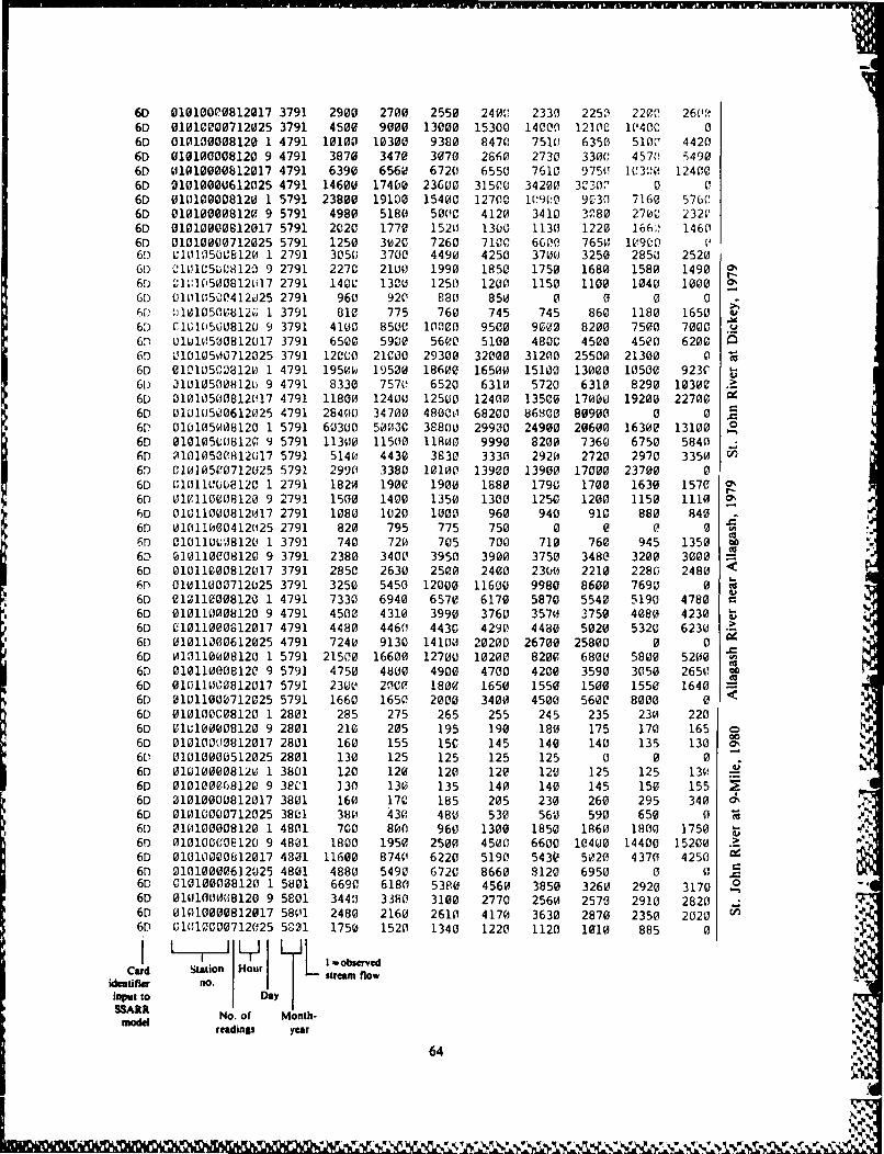
6D 01010000812017 3791 2900 2700 2550 240'! 2330 2253) 2200 26(26D 01010000712025 3791 4500 9000 13000 15300 14000 121C0 1('40C 06D 010100008120 1 4791 10100 10300 9380 8470 7510 6350 510C 44206D 010100008120 9 4791 3870 3470 3070 2860 2730 330C 45701 54906D 01010000812017 4791 6390 6560 6720 6550 7610 9750 IC3;10 124006D 01010000612025 4791 14600 17400 23600 31500 34200 31030 0 06D 010100008120 1 5791 23800 19100 15400 12700 1C9(0 9030 7160 57606D 010100008120 9 5791 4980 5180 5000 4120 3410 3280 2700 232V6D 01010000812017 5791 2020 1770 1520 1300 1130 1220 1661! 14606D 01010000712025 5791 1250 3020 7260 7100 6600 7650 19P0 06) 010105008120 1 2791 3050 3700 4490 4250 3700 3250 2850 252061) 01=5 508120 9 2791 2270 2100 1990 1850 1750 1680 1580 14906r) 1.,1O 5,0812oI7 2791 1400 1300 1250 1200 1150 1100 1040 1000 oGD 0101';5'0412J25 2791 960 920 880 850 0 0 0 060 P I10500812 1 3791 810 775 760 745 745 860 1180 16506, C010(5008120 9 3791 4100 8500 10000 9500 900 8200 7500 70006' UI10500812017 3791 6500 5900 56V0 5100 4800 4500 4500 6200 IM6D 01010500712025 3791 120C0 21000 29300 32000 31200 25500 21300 06D 010105CO8120 1 4791 195M) 19500 186V0 16500 15100 13000 10500 9230 ,61) 310105008120 9 4791 8330 757V 6520 6310 5720 6310 8290 10300 .-

6D 01010500812(117 4791 11800 124(00 12500 12400 13500 17000 19200 22700 "C6D 0101(1500612025 4791 28400 34700 48000- 68200 86800 80900 0 0 =

6P' 010105008120 1 5791 60300 50000 38800 29900 24900 20600 16300 13100 o6D 010105U08120 9 5791 11300 11500 11800 9990 8200 7360 6750 5840 .6D 0101050V812(;17 5791 5140 4430 3830 3330 2920 2720 2970 335060 0110050712025 5791 2990 3380 10100 13900 13900 17000 23700 06D 011110008120 1 2791 1820 1900 1900 1880 1790 1700 1630 1570 o16D 0lV10008120 9 2791 1500 1400 1350 1300 1250 1200 1150 1110 o6D 010110008120117 2791 1080 1020 1000 960 940 910 880 8406D 01011000412025 2791 820 795 775 750 0 0 P 06r 0101100,8120 1 3791 740 720 705 700 710 760 945 13506D 010110C08120 9 3791 2380 3400 3950 3900 3750 3480 3200 3000 _9

6D 01011000812017 3791 285C 2630 2590 2400 2300 2210 2280 2480 <60 01011000712025 3791 3250 5450 12000 11600 9980 8600 7690 0 06D 010110008120 1 4791 7330 6940 6570 6170 5870 5540 5190 4780 C

6D 010110008120 9 4791 4500 4310 3990 3760 3570 3750 4080 42306D C1011000612017 4791 4480 4460 4430 4290 4480 5020 5320 6230 --6) 01011300612025 4791 724w 9130 14100 20200 26700 25800 0 06D 013110008120 1 5791 21500 16600 12700 10200 8200 6800 5800 52006D 010110008120 9 5791 4750 4800 4900 4700 4200 3590 3050 26506D 0101100,0812017 5791 2300 200 1800 1650 1550 1500 1550 1640 --6D 01011000712025 5791 1660 1650 2000 3400 4500 5600 8000 0 <

6D 010100008120 1 2801 285 275 265 255 245 235 230 2206D 010100008120 9 2801 210 205 195 190 180 175 170 165 O6D 01010000812017 2801 160 155 150 145 140 140 135 130 do6L" 010100O0512025 2801 130 125 125 125 125 0 0 06D 010100008120 1 3801 120 120 120 120 120 125 125 130 -260 010100018120 9 3801 130 130 135 140 140 145 150 155 "

6D 31010000812017 3801 160 170 185 205 230 260 295 340 o.6D 01010000712025 3801 380 430 480 530 560 590 650 0 .6[) 010100008120 1 4801 700 800 960 1300 1850 1860 1800 1750 -60 0101000120 9 4801 1800 1950 2500 4500 6600 10400 14400 15200 .-6D 01010000812017 4301 11600 8740 6220 5190 543V 5020 4370 4250 06D 01010009612025 4801 4880 5490 6720 8660 9120 6950 0 060 010100008120 1 5801 6690 6180 5380 4560 3850 3260 2920 3170 o6D 010100008120 9 5801 344'3 3380 3100 2770 2560 2570 2910 2820 N6D 01010000812017 5801 2480 2160 2610 4170 3630 2870 2350 20206D 01010000712025 5001 1750 1520 1340 1220 1120 1010 885 0

Card Station Hour Lui~od reding '7' streaim flowidewifier no.

input to DaySSARR No. of Month-mdlreadinlp year 'N,

64 %

7s~

6D 010105008120 1 2801 630 613 580 560 540 525 500 49061 010105008120 9 2801 470 460 450 430 420 410 395 3856D 01010500812017 280i1 380 365 355 345 340 335 330 3256D 01010500512025 2801 320 315 310 310 305 0 3 0 -6D 010105008120 1 3801 300 300 295 30 300 305 305 3106D 010105008120 9 3801 310 315 320 325 330 345 355 370 -6D 01010500812017 3801 385 425 470 525 600 680 760 8506D 0101050712025 38VI 950 1000 1100 1200 1250 13010 1400 0 -

6D 0101015008120 1 4801 1500 1700 1900 2150 2750 36'50 3750 3700 c6D 010105008120 9 4801 3700 4050 biOO 9000 14000 Z2500 29400 337006D 01010500812017 4801 26700 1913:) 13800 11000 12600 I1030 8870 84406D 01010500612025 48VI 9760 11300 12800 15900 16200 14200 0 06D 31010500812.' 1 5801 12700 12(00 10700 9140 7730 6560 5870 6350 .6D 010105008120 9 5801 7190 6900 6230 5590 5050 5200 5940 5950 -6D 01010500812017 5801 5200 4600 4360 6060 7070 6140 5090 4240 46D 01010500712025 5801 3660 3190 2840 2590 2380 2190 2020 06D 01011001812(4 1 2801 380 360 375 370 365 365 36; 3606D 010110008120 9 2801 355 35e 350 350 345 345 340 340 006') 01011000812017 2801 340 335 330 330 325 325 325 320 -k

6,) 01011(00512025 2801 320 320 315 315 310 0 0 0 C60 010110008120 1 3801 310 305 305 300 300 305 305 305 t6D 010110008120 9 3801 305 305 310 310 310 310 310 315 c6;) 01011000812017 380I 315 320 325 3301 335 345 360 3856, 01011000712025 3801 4110 440 475 520 570 630 690 0 ,6P 010110008120 1 4801 760 850 950 1020 1120 1200 1310 1450 v6D 010110008120 9 4801 1700 2100 2700 3700 500 6300 7200 P613 =6D 010111000812017 4801 6860 5740 4780 4200 4320 3630 3430 34806D 01011000612025 4801 3700 3890 428(0 4520 4290 4070 0 0 '6D 01P1100081201 1 5811 3910 3790 3610 3390 3130 2910 2790 2990 .6D 01CI10039120 9 5801 3250 3280 304 2770 2590 2770 3130 2862 "to6D ('10 1I 0 12017 58Ji 2550 2350 2500 2720 2650 2530 2380 2230 .56D 31011000712025 5801 2030 1830 1730 1610 149C 1410 1340 ,

I LrI oseveCard station Hou L sr oem'rfldidentifier no.

input to Dy .-

SSARR No. of Month-mode readings year

65

% -

Wind Speed

4D 1 120 1 2798 34 34 47 34 58 69 34 22 58 34 47 11 34 584D 1 12015 2798 34 47 58 34 22 22 00 22 34 34 22 11 114D 1 120 1 3798 11 22 22 11 11 22 00 22 11 11 22 69 22 474D 1 1215 3798 58 22 34 34 22 34 11 11 11 34 22 34 69 224D 1312029 3798 11 22 114D 1 120 1 4798 34 22 11 22 22 11 58 22 00 34 69 58 34 224D 1 12015 4798 22 22 22 22 22 22 11 00 22 22 22 34 47 474D 1212029 4798 00 114D 1 120 1 5798 58 47 22 11 58 114 81 22 47 69 22 69 34 004D 1 12015 5798 47 11 22 45 45 45 45 67 45 22 67 67 45 224D 1312029 5798 45 45 224D 1 120 1 2808 47 34 34 22 34 11 11 11 11 22 11 11 47 474D 1 12015 2808 58 00 58 69 92 11 34 11 22 22 34 34 11 224D 1112029 2808 474D 1 120 1 3808 58 22 11 34 22 47 34 11 11 22 47 69 11 344D 1 12015 3808 58 47 22 34 47 11 34 58 34 11 22 22 22 224D 1312029 3808 22 22 224D 1 120 1 4808 11 22 22 34 22 22 69 47 34 58 11 47 344D 1 12015 4808 47 47 34 47 58 69 58 47 11 22 22 004D 1212029 4808 22 004D 1 120 1 5808 22 45 45 67 67 45 67 45 22 45 67 90 45 224D 1 12015 5808 22 47 22 47 34 22 58 47 22 34 34 47 47 224D 1312029 5808 34 22 22

Card Sttion H H OWCode for Wind speed (m/h)idenifier no. Diy ya wind speedinput to Mon (m/h xxx.x)SSARR

No. of

modd re s/

carddefanlt-14

66

IMONW4

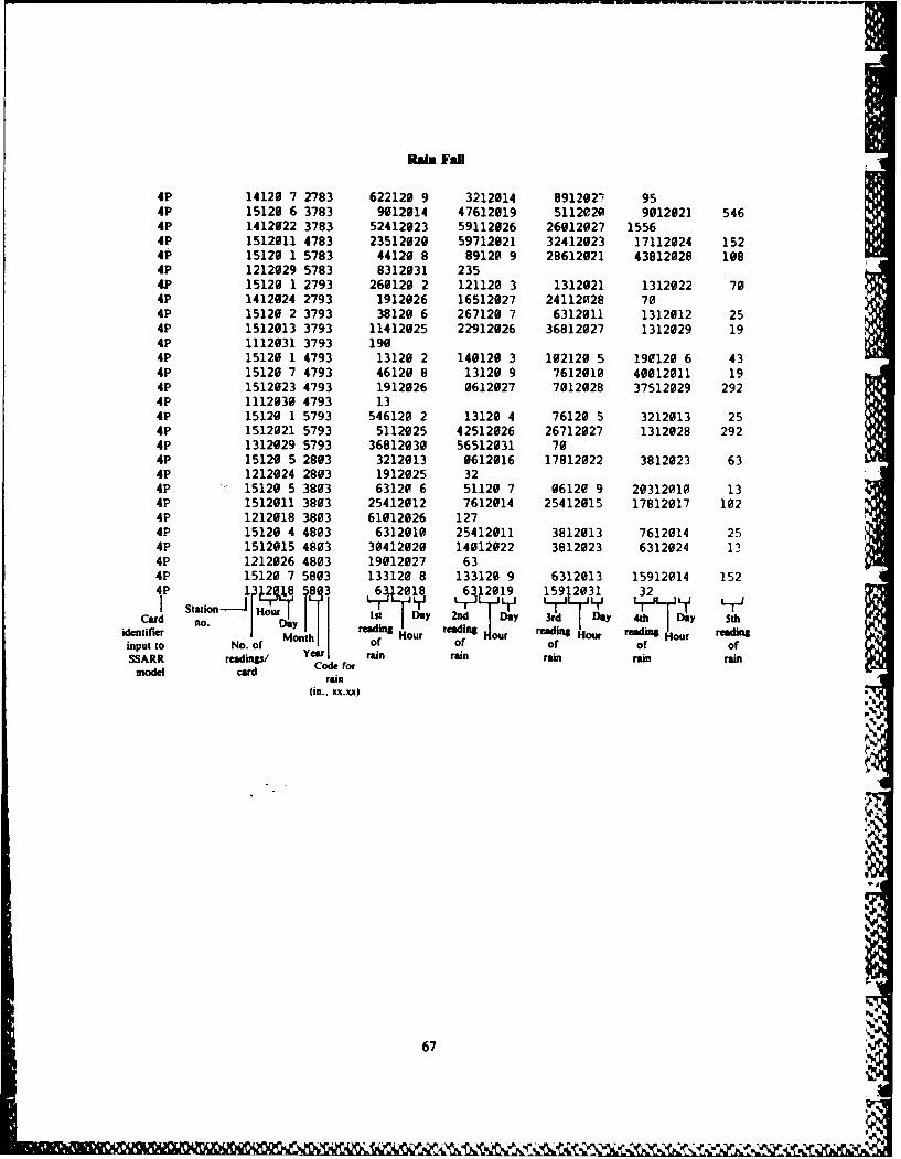
Ral Fall

4P 14120 7 2783 622120 9 3212014 891202' 954P 15120 6 3783 9012014 47612019 5112020 9012021 5464P 1412022 3783 52412023 59112026 26012027 15564P 1512011 4783 23512020 59712021 32412023 17112024 1524P 15120 1 5783 44120 8 89120 9 28612021 43812028 1084P 1212029 5783 8312031 2354P 15120 1 2793 260120 2 121120 3 1312021 1312022 704P 1412024 2793 1912026 16512027 24112028 704P 15120 2 3793 38120 6 267120 7 6312011 1312012 254P 1512013 3793 11412025 22912026 36812027 1312029 194P 1112031 3793 1904P 15120 1 4793 13120 2 140120 3 102120 5 190120 6 434P 15120 7 4793 46120 8 13120 9 7612010 40012011 194P 1512023 4793 1912026 0612027 7012028 37512029 2924P 1112030 4793 134P 15120 1 5793 546120 2 13120 4 76120 5 3212013 254P 1512021 5793 5112025 42512026 26712027 1312028 2924P 1312029 5793 36812030 56512031 704P 15120 5 2803 3212013 0612016 17812022 3812023 634P 1212024 2803 1912025 324P 15120 5 3803 63120 6 51120 7 06120 9 20312010 134P 1512011 3803 25412012 7612014 25412015 17812017 1024P 1212018 3803 61012026 1274P 15120 4 4803 6312010 25412011 3812013 7612014 254P 1512015 4803 30412020 14012022 3812023 6312024 134P 1212026 4803 19012027 634P 15120 7 5803 133120 8 133120 9 6312013 15912014 1524P'JL 18.81 6-U203 } 1 8 109 15912031 3

a stationY Hu Ist , 2nd k

identifier Month I Hour I. d ur eadin Hour reading Hourinput to No. of I of of of of ofSARR readings/ er an rain rain rain rain

model card rain

(in., x.xx)

67

~ C k ~ ~ y 2~ ? Aw x A

Air Temperature

4! 1 12.' 1 27P4 32 -4t; -94 -58 -58 -31 156 E6 59 -67 -31 122 66 -224r' 1 12215 27b4 248 131 C6 185 68 50 104 194 167 156 122 266 257 1404D 1 128 1 3784 122 176 59 95 50 122 152 149 140 158 158 266 15F 2484D 1 12015 3764 302 104 32 59 158 212 149 262 194 176 212 176 284 33h4D 1312029 3784 329 266 266 0 ( (0 ( (1 0 1 10 0 ;i4D 1 120 1 4784 176 239 140 176 320 320 284 32(0 338 356 356 356 374 3744D 1 12015 47E4 347 374 347 363 337 411 344 337 352 363 374 374 392 3924D 1212029 4784 392 292 r. U ( ( 0 1 0 0 0 0 0 04D 1 128 1 5784 320 401 392 383 410 410 428 464 410 5010 482 509 516 5(194D 1 12015 5784 572 545 59C 545 518 473 464 455 473 486 566 56 549 6504D 1312029 5784 643 636 5 96 0 8 0 ( (1 (0 C; (0 V' (1 r,41 1 120 1 2794 262 214 135 176 52 63 77 146 -63-149-140-142-130-134D 1 121415 2794-121-11(-1401 -85 -25 113 275 169 164 32C 175 135 211 3334C 1 128 1 3794 220 223 299 362 405 423 358 34V1 326 257 308 124 774 3334D 1 12015 3794 149 70 103 283 31U 351 409 421 463 446 3F"8 353 221 2254D 1312029 3794 297 362 3564T 1 120 1 4794 306 3 1 364 360 301 324 296 225 243 324 324 351 416 4C34D 1 12C15 4794 353 515 335 311 385 445 515 506 423 425 443 576 526 5624D 1212029 4794 515 5134D 1 12V 1 5794 513 428 5V'(! 455 399 399 441 497 655 486 490 553 5901 5564D 1 12015 5794 610 596 704 576 b52 635 655 488 526 569 493 463 576 5294D 1312029 5794 548 560 56940 1 12 1 204 1838178 47 9588 1876 16-23 26 9731 7741 1 12015 2804 -40 32 45 74 232 223 227 11 1(1 72 145 -5b -13 314D 1112829 2804 -2540 1 120 1 3804 7 -20 59 106 180 153 149 85 194 135 218 34 32 1664D 1 12015 3804 135 88 90 245 250 124 2301 295 360 279 326 346 333 38004D 1312(129 3804 3H2 326 290"4D 1 120 1 4804 275 346 371 360 362 299 214 355 446 446 391 38V 432 4014D 1 12815 4804 470 401 301 335 310 365 387 245 346 391 466 445 41C 3914D 12121,29 4804 416 4724D 1 120 1 58(04 475 526 5010 481 351 410 475 401 436 436 443 605 495 5204D 1 12815 5PV4 43 475 466 515 605 481 517 594) 490 486 5'AC 455 452 461

1312029 5804 446 486 590

Card . Code Air temperature readingsidentifier Day Ye or air

in p u t to N o . o f M o n t h t e m p e r a t u r e - -

SSARR reading/ (F, xxx.x)model card,

default 14

68

%

I

t

A facsimile catalog card in Library of Congress MARC format is re-produced below.

Merry, Carolyn J.Use of Landsat digital data for snow cover mapping in the Upper

Saint John River Basin, Maine / Carolyn J. Merry and Michael S. Mil-ler. Hanover, N.H.: U.S. Army Cold Regions Research and Engineer-ing Laboratory; Springfield, Va.: available from National TechnicalInformation Service, 1987.

v, 74 p., illus.; 28 cm. (CRREL Report 87-8.)Bibliography: p. 52.1. Hydrolgic modeling. 2. Landsat. 3. Remote sensing. 4. Runoff. 5.

Snow cover. 6. Snow water equivalent. I. Miller, Michael S. I. UnitedStates. Army. Corps of Engineers. Ill. Cold Regions Research andEngineering Laboratory, Hanover, N.H. IV. Series: CRREL Report87-8.

mill

000000

F%~