Embed Size (px)
Citation preview
Smart Grid and
Customer Transactions:
The unrealized Benefits
of Conformance
Authors
Girish Ghatikar – LBNL
Ed Koch – Honeywell Building Solutions
Rolf Bienert – OpenADR Alliance
Jim Zuber - QualityLogic
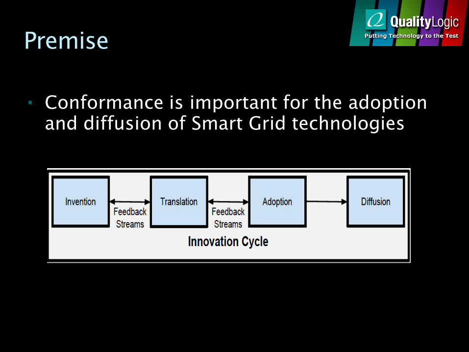
Premise
Conformance is important for the adoption and diffusion of Smart Grid technologies
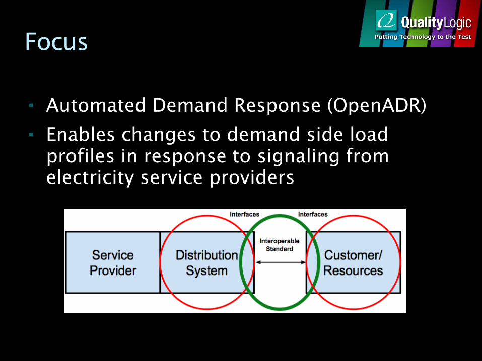
Focus
Automated Demand Response (OpenADR)
Enables changes to demand side load profiles in response to signaling from electricity service providers
Topics
OpenADR Origins
Technology Primer
Conformance Requirements
Testing
Conclusions
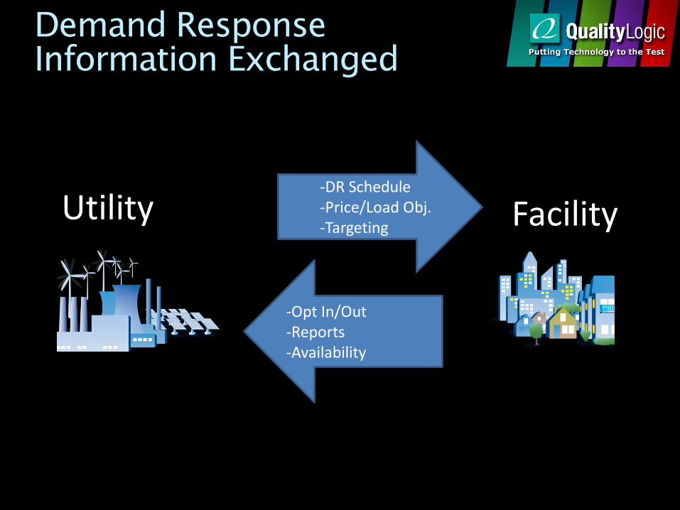
Demand Response Information Exchanged
-DR Schedule -Price/Load Obj. -Targeting
-Opt In/Out -Reports -Availability
Utility Facility
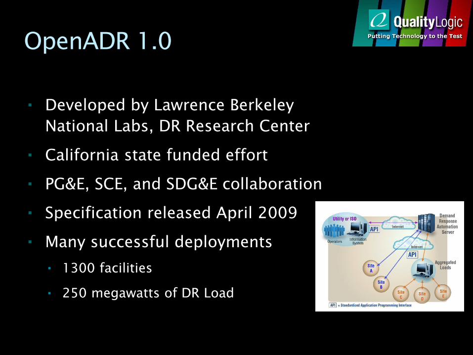
OpenADR 1.0
Developed by Lawrence Berkeley
National Labs, DR Research Center
California state funded effort
PG&E, SCE, and SDG&E collaboration
Specification released April 2009
Many successful deployments
1300 facilities
250 megawatts of DR Load
OpenADR 2.0
NIST Smart Grid harmonization project
initiated in 2009
Priority Action Plans (PAPs) to work on
common standards for price models, schedule
representation, and standard DR Signals
OpenADR Alliance formed in 2010 to evolve
work done on OpenADR 1.0 into an recognized
standard and to implement a formal
certification process
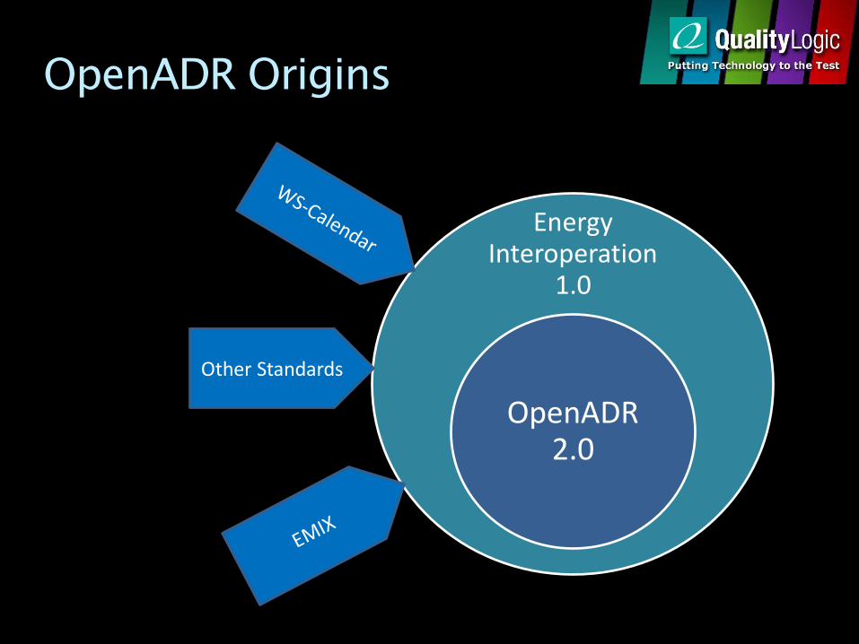
OpenADR Origins
Energy Interoperation
1.0
OpenADR 2.0
Other Standards
VENs and VTNs
Two actors in OpenADR communication exchanges
Virtual Top Nodes (VTN)
Transmit events other nodes
Virtual End Nodes (VEN)
Receive events and respond to them
Control demand side resources
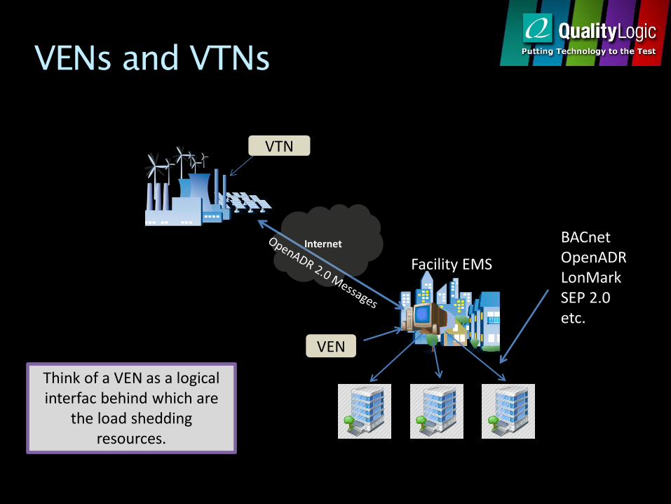
VENs and VTNs
VTN
VEN
Internet BACnet OpenADR LonMark SEP 2.0 etc.
Think of a VEN as a logical interfac behind which are
the load shedding resources.
Facility EMS

Services
Event Service
Send and Acknowledge DR Events
Opt Service
Define temporary availability schedules
Report Service
Request and deliver reports
Registration Service
VEN Registration, device information exchange
Profiles
A Profile
Simple devices, limited event service only
B Profile
More robust devices, all services supported

Transports, Data Models
IP based HTTP and XMPP transports
XML Payloads
Push and Pull exchange patterns
Robust open source libraries available for implementation
Security
Exchange of Client and Server x.509v3 certificates
TLS 1.2
SHA256 ECC or RSA ciphers
Optional XML payload signatures
Robust out of the box security

A and B Profiles
Interoperability
VTNs must support all features and functions
VENs have some limited optionality
Backwards Compatibility
VTNs must concurrently communicate with both A and B profile VENs
VTNs must upgrade to latest profile version to maintain certification
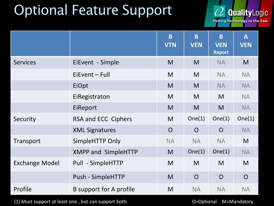
Optional Feature Support
B VTN
B VEN
B VEN
Report
A VEN
Services EiEvent - Simple M M NA M
EiEvent – Full M M NA NA
EiOpt M M NA NA
EiRegistraton M M M NA
EiReport M M M NA
Security RSA and ECC Ciphers M One(1) One(1) One(1)
XML Signatures O O O NA
Transport SimpleHTTP Only NA NA NA M
XMPP and SimpleHTTP M One(1) One(1) NA
Exchange Model Pull - SimpleHTTP M M M M
Push - SimpleHTTP M O O O
Profile B support for A profile M NA NA NA
(1) Must support at least one , but can support both. O=Optional M=Mandatory
OpenADR Schema & Spec
XML Schema
Specifies payload structure, data types, enumerated values, etc.
Profile Specifications
Narrative description of protocol behavior
Formal conformance rules that specify..
Conformance (business) Rules
Security
Transport requirements
PICS Document
Protocol Implementation Conformance Statement (PICS)
Listing of all testable requirements
Manufacturer declares conformance prior to certification
Indication of supported features directs test cases run during certification
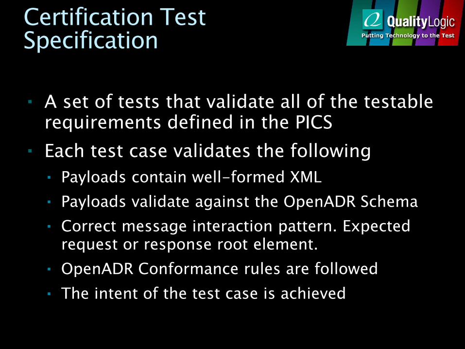
Certification Test Specification
A set of tests that validate all of the testable requirements defined in the PICS
Each test case validates the following
Payloads contain well-formed XML
Payloads validate against the OpenADR Schema
Correct message interaction pattern. Expected request or response root element.
OpenADR Conformance rules are followed
The intent of the test case is achieved
Test Harness
Implements all test cases
Plays one side (VEN or VTN) in the OpenADR message exchange
Available to adopters prior to certification
Self test mechanism provide reference implementation
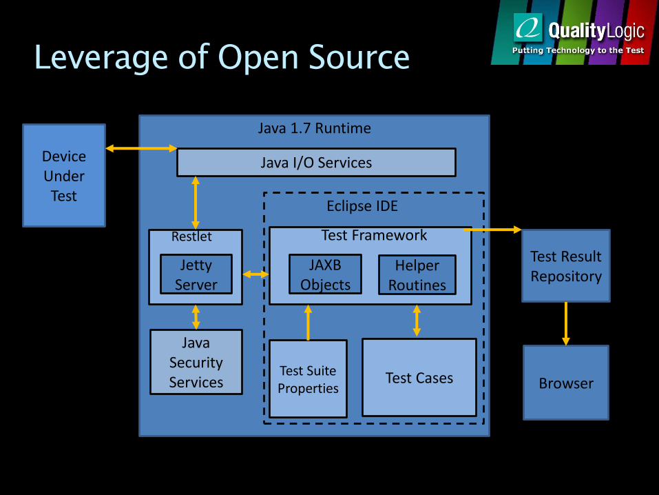
Leverage of Open Source
Device Under
Test
Test Result Repository
Browser
Java 1.7 Runtime
Java I/O Services
JAXB Objects
Jetty Server
Helper Routines
Test Framework
Test Suite Properties
Test Cases
Restlet
Eclipse IDE
Java Security Services
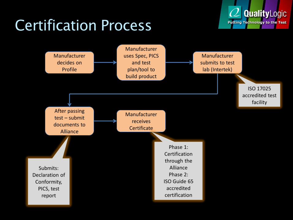
Certification Process
Manufacturer decides on
Profile
Manufacturer uses Spec, PICS
and test plan/tool to
build product
Manufacturer submits to test lab (Intertek)
After passing test – submit documents to
Alliance
Manufacturer receives
Certificate
ISO 17025 accredited test
facility
Submits: Declaration of
Conformity, PICS, test
report
Phase 1: Certification through the
Alliance Phase 2:
ISO Guide 65 accredited
certification
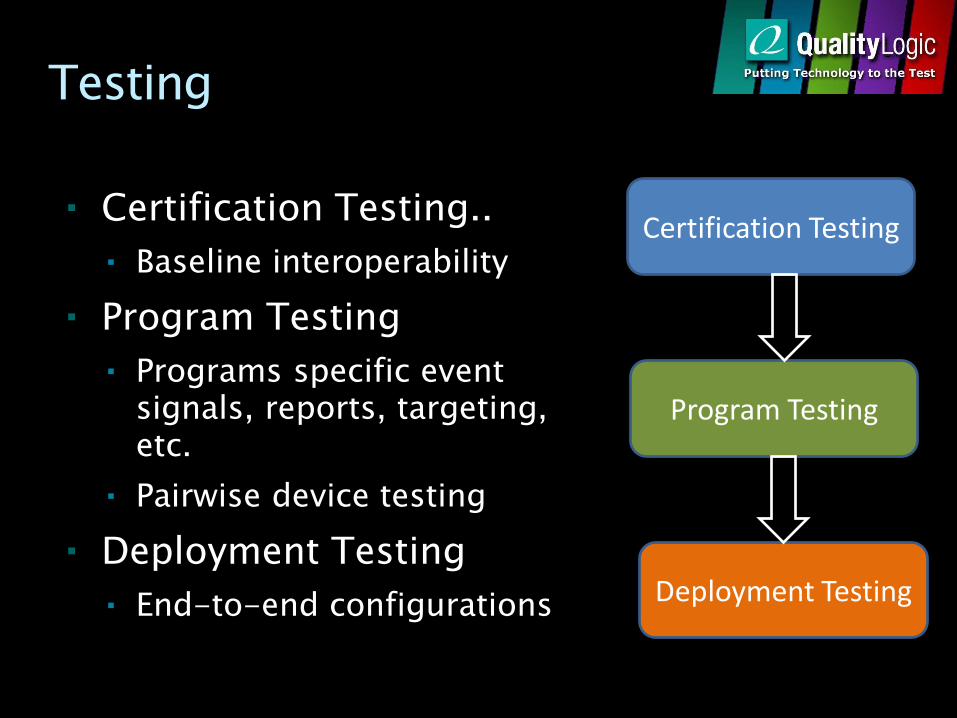
Certification Testing..
Baseline interoperability
Program Testing
Programs specific event signals, reports, targeting, etc.
Pairwise device testing
Deployment Testing
End-to-end configurations
Testing
Certification Testing
Program Testing
Deployment Testing
OpenADR Success
Well defined requirements and robust requirements result in…
120 OpenADR Alliance Member companies
Over 60 certified devices available
Strong national and international interest
Many trail deployments in progress
OpenADR being written into regulations
Broad perception that OpenADR VENs and VTNs are interoperable
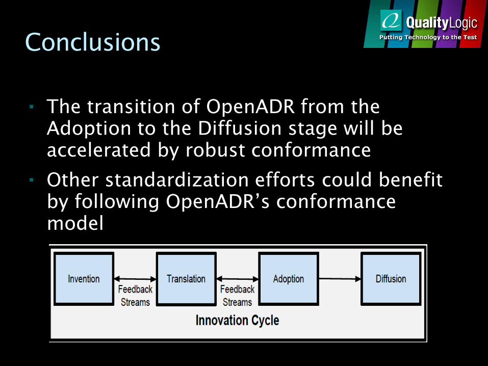
Conclusions
The transition of OpenADR from the Adoption to the Diffusion stage will be accelerated by robust conformance
Other standardization efforts could benefit by following OpenADR’s conformance model

Questions?

Simulation and Experimental Performance Analysis of Micro-grid
Based Distributed Energy ResourcesElectrical Engineering & Telecommunications
Yunqi Wang
24 November 2014

Outline• 1. Introduction
• 2. Model of simulation system
• 3. Impact of micro-grid operation modes
• 4. Impact of battery storage capacity
• 5.Impact of DG penetration level
• 6. Experimental study
• 7.Conclusion

Background
1.Definition of the Micro-grid-- a cluster of loads and micro-sources operation as a single
controllable system providing both power and heat to its local area.
2.Operation mode of the micro-grid--islanded mode and grid-connected mode
3.Transient stability of micro-grid--voltage and frequency should always be maintained within a
permissible limit--distributed generator need to be operated during these periods

Research Reason
-- Analysis of behaviors of distribution systems during transients is especially difficult.
-- The DGs output power is affected by many factors and could be changed rapidly and irregularly.
-- The DG output change may lead the undesirable impact on the component in the main network.

Research Objective
• To compare the dynamic response of a micro-grid when system load demand suddenly decreases.
• --Simulation: The simulations are carried out to study the micro-grid transients with different operation modes, different sizes of energy storage and different DG penetration levels.
• --Experiment: The results are validated using a laboratory setup of a micro-grid, having a mix of PV, wind turbine and battery storage.
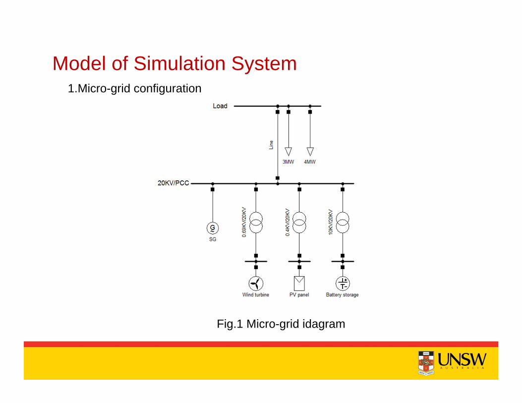
Model of Simulation System1.Micro-grid configuration
Fig.1 Micro-grid idagram
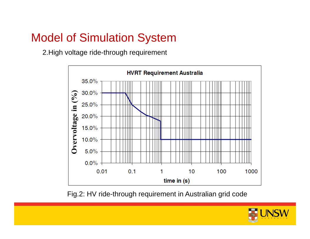
Model of Simulation System2.High voltage ride-through requirement
Fig.2: HV ride-through requirement in Australian grid code

Impact of micro-grid operation mode• Scenario 1: In the grid-connected mode
Fig.3 PCC voltage, grid-connected mode
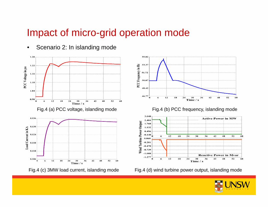
Impact of micro-grid operation mode• Scenario 2: In islanding mode
Fig.4 (a) PCC voltage, islanding mode Fig.4 (b) PCC frequency, islanding mode
Fig.4 (c) 3MW load current, islanding mode Fig.4 (d) wind turbine power output, islanding mode

Impact of the Battery Storage Size• Battery capacity chosen
4MW, 0.8pf lagging
Assuming the battery efficiency is about 70%. Note that some power losses also incur in the transmission lines.
Therefore, 10MVA is chosen as the battery power rating in the simulation .
Furthermore, the generator transient may also lead to some power unbalance. Thus, a second simulation with 30MVA battery is also considered
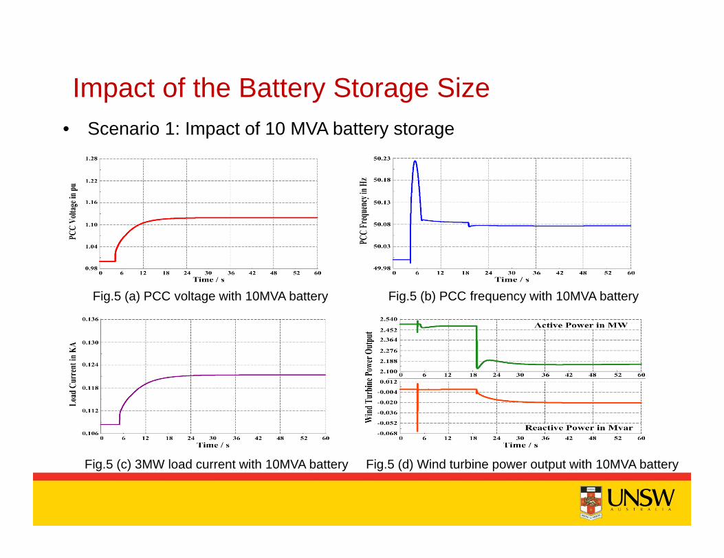
Impact of the Battery Storage Size• Scenario 1: Impact of 10 MVA battery storage
Fig.5 (a) PCC voltage with 10MVA battery Fig.5 (b) PCC frequency with 10MVA battery
Fig.5 (c) 3MW load current with 10MVA battery Fig.5 (d) Wind turbine power output with 10MVA battery
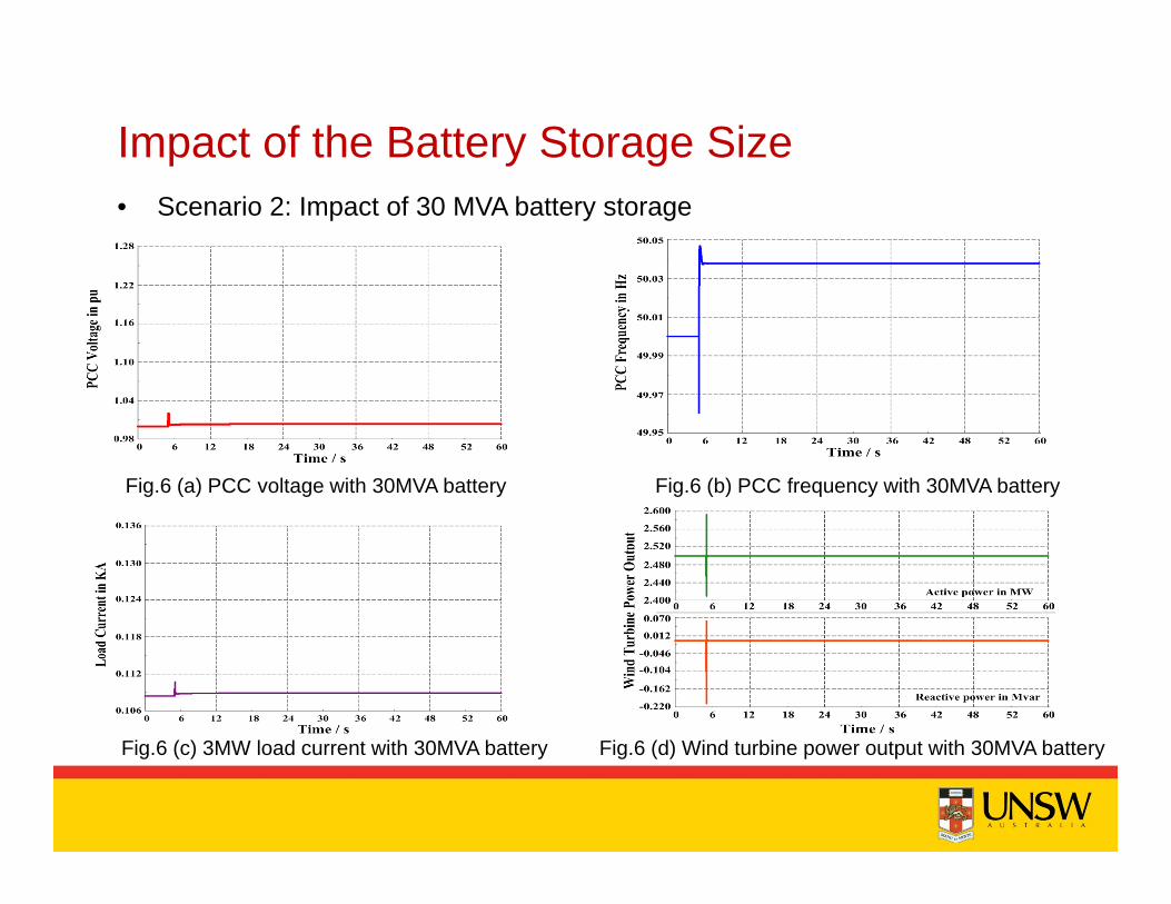
Impact of the Battery Storage Size• Scenario 2: Impact of 30 MVA battery storage
Fig.6 (a) PCC voltage with 30MVA battery Fig.6 (b) PCC frequency with 30MVA battery
Fig.6 (c) 3MW load current with 30MVA battery Fig.6 (d) Wind turbine power output with 30MVA battery
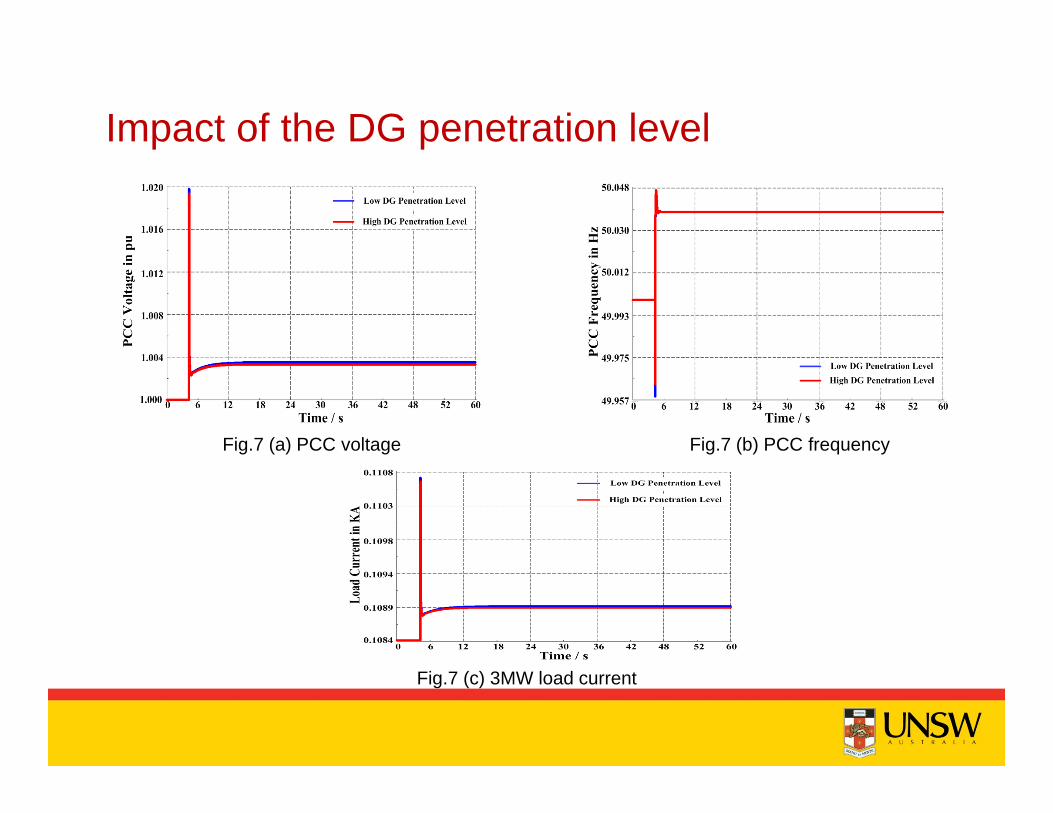
Impact of the DG penetration level
Fig.7 (a) PCC voltage Fig.7 (b) PCC frequency
Fig.7 (c) 3MW load current
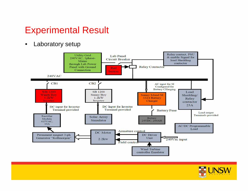
Experimental Result• Laboratory setup
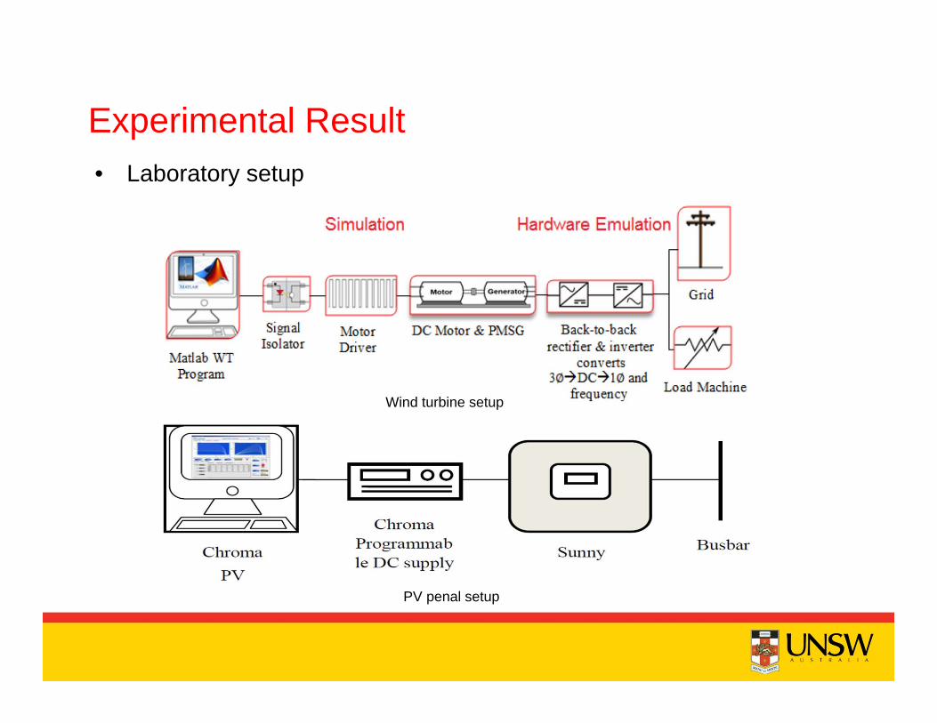
Experimental Result• Laboratory setup
Wind turbine setup
PV penal setup
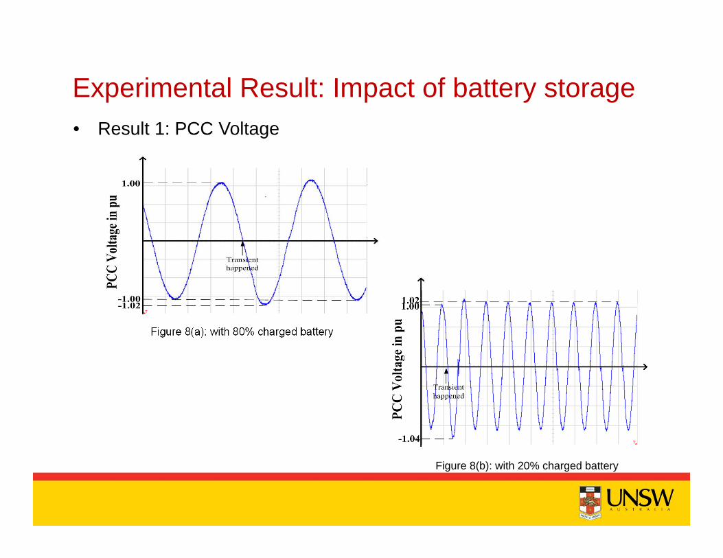
Experimental Result: Impact of battery storage• Result 1: PCC Voltage
Figure 8(b): with 20% charged battery
Figure 8(a): with 80% charged battery
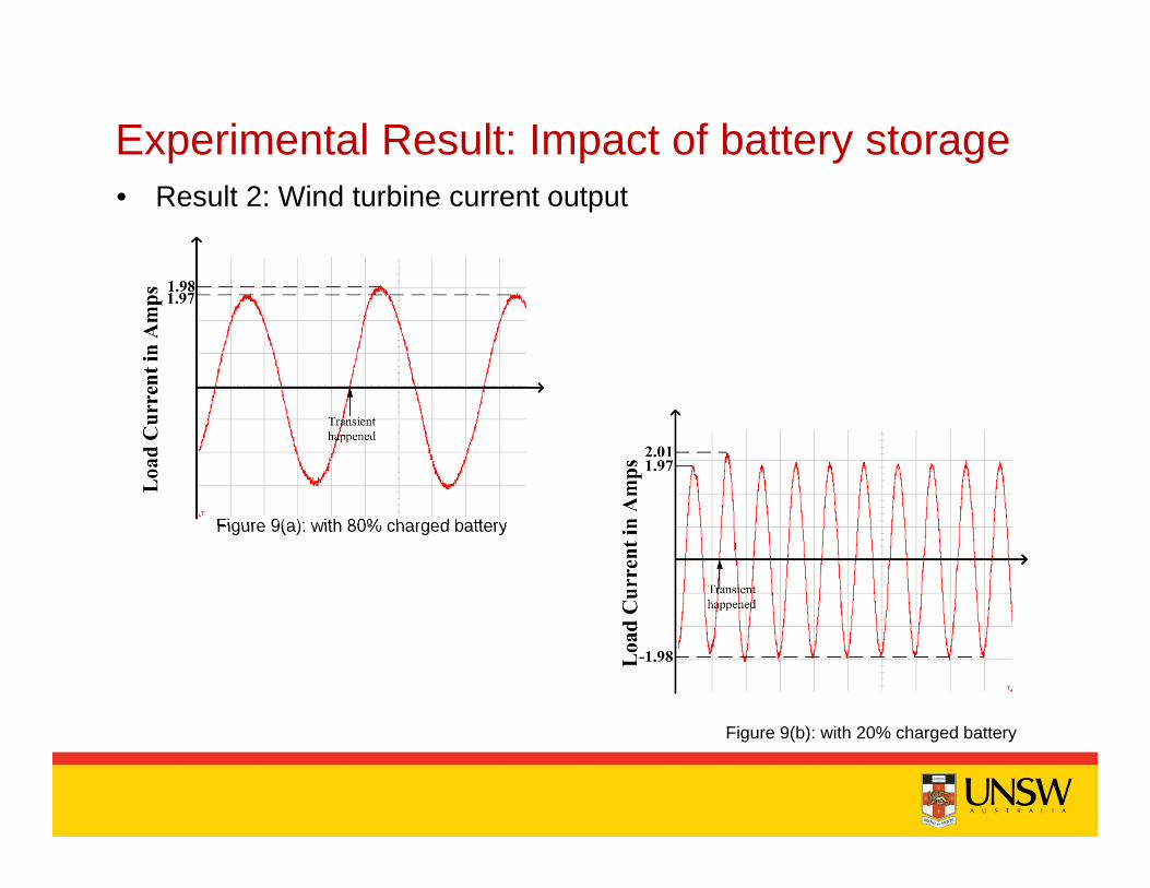
Experimental Result: Impact of battery storage• Result 2: Wind turbine current output
Figure 9(a): with 80% charged battery
Figure 9(b): with 20% charged battery
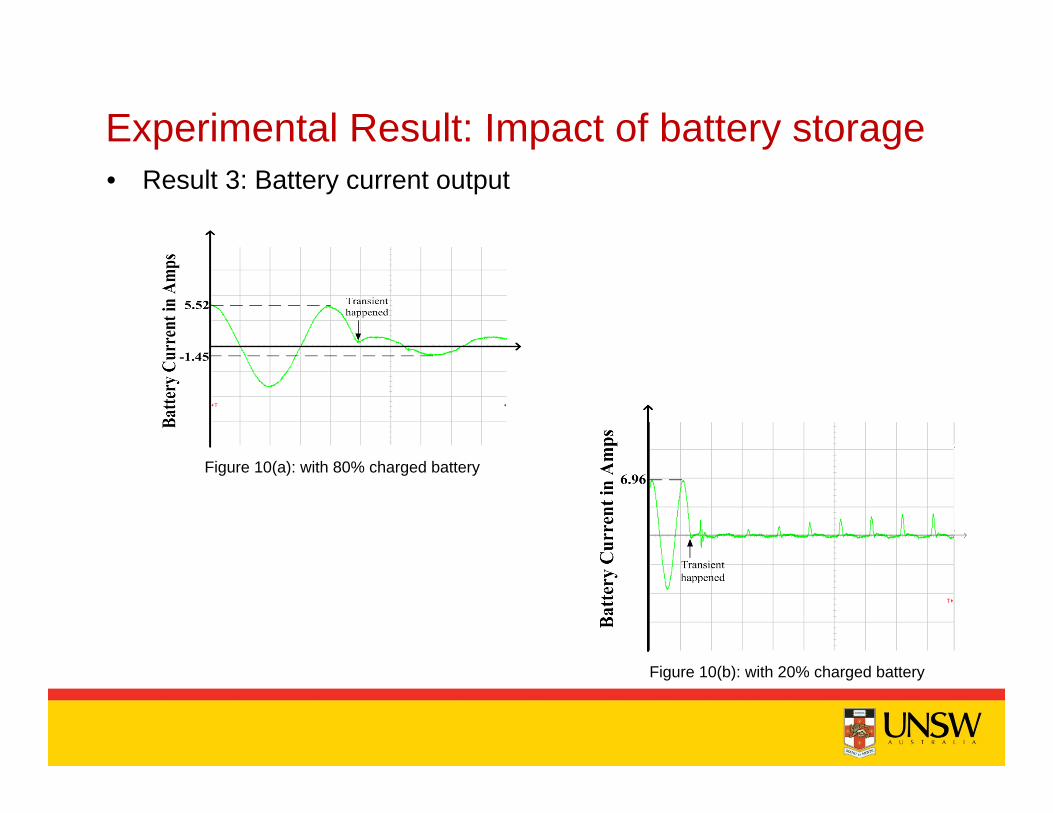
Experimental Result: Impact of battery storage• Result 3: Battery current output
Figure 10(a): with 80% charged battery
Figure 10(b): with 20% charged battery
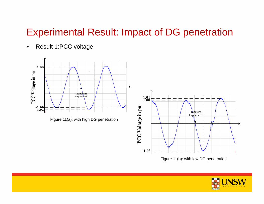
Experimental Result: Impact of DG penetration • Result 1:PCC voltage
Figure 11(a): with high DG penetration
Figure 11(b): with low DG penetration

Experimental Result: Impact of DG penetration • Result 2:wind turbine current output
Figure 12(a): with high DG penetration
Figure 12(b): with low DG penetration
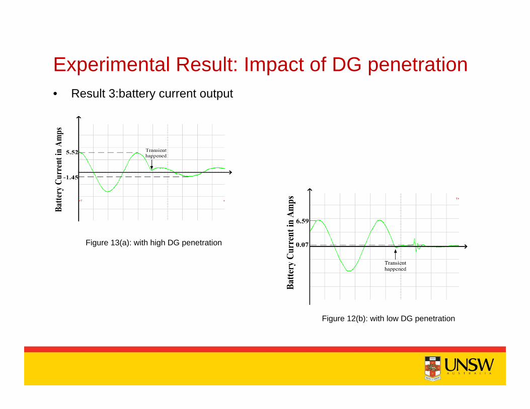
Experimental Result: Impact of DG penetration • Result 3:battery current output
Figure 13(a): with high DG penetration
Figure 12(b): with low DG penetration
Conclusion• When the micro-grid operates in islanding mode, the load demand
changes affect the system stability significantly as they can cause apower rush during the disturbance;
• This problem can be solved by installation of storage unit. The powerrush can be absorbed by this device and the micro-grid dynamicresponse is substantially improved. Nevertheless, the transientcaused by the rotating machine should also be considered whendetermining the capacity of the battery. Otherwise, the micro-grid willface the high voltage situation;
• The DG penetration level also has impact on the micro-grid transient.Increasing the DG penetration level can reduce the overshootingduring the transient and enhance the system transient performanceas more power rush can be absorbed by both SG and DG.

Thank you

Advanced Metering Infrastructure’s Measurement of Working, Reflected, and Detrimental Active Power in Microgrids By: Tracy N. Toups, Leszek S. Czarnecki Louisiana State University Nov. 23rd , 2014
IGESC 2014 IEEE Green Energy and Systems Conference

Introduction
Power system economics is very important.
Current billing standards are 100 years old.
Can these standard still be used for today’s society?
IGESC 2014 IEEE Green Energy and Systems Conference

Traditional Active Power
Main component of energy bills is the cost of energy delivered to the customer in a month.
Where Wa is the active energy and P is the active power.
Analog meters are based upon this principle.
0
month
aW Pdt= ∫
IGESC 2014 IEEE Green Energy and Systems Conference
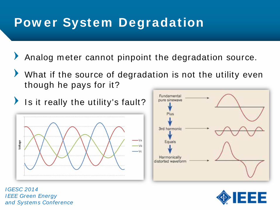
Power System Degradation
Analog meter cannot pinpoint the degradation source.
What if the source of degradation is not the utility even though he pays for it?
Is it really the utility's fault?
IGESC 2014 IEEE Green Energy and Systems Conference
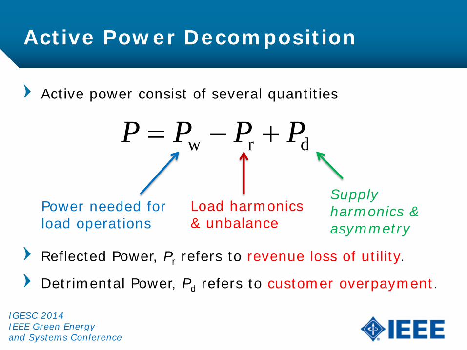
Active Power Decomposition
Active power consist of several quantities
Reflected Power, Pr refers to revenue loss of utility.
Detrimental Power, Pd refers to customer overpayment.
w r dP P P P= − +
Supply harmonics & asymmetry
Load harmonics & unbalance
Power needed for load operations
IGESC 2014 IEEE Green Energy and Systems Conference

Microgrids and Advanced Metering Infrastructure
Due to the small size of microgrids, they tend to be low MVA systems which makes them especially susceptible to distortion and asymmetry.
Additionally, most microgrids tend to integrate renewable sources of energy which uses power converters that are major sources of distortion.
A new concept of working active power can easily be integrated with the use of the advanced metering infrastructure’s (AMI) microprocessor based meters.
IGESC 2014 IEEE Green Energy and Systems Conference

Main Points of the Research
Active power is a composite concept that needs further decomposition.
One party (utility or customer) is not being accurately compensated financially by the other party.
A new concept of working active power can reveal the disparity and pinpoint degradation source.
Can be easily integrated into microgrid systems.
IGESC 2014 IEEE Green Energy and Systems Conference
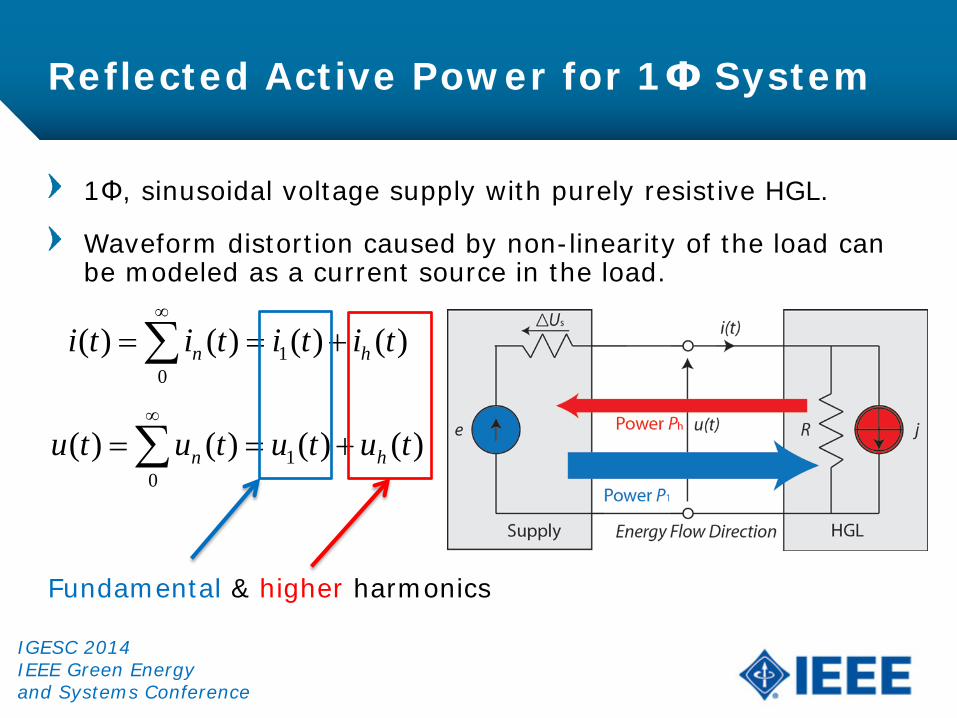
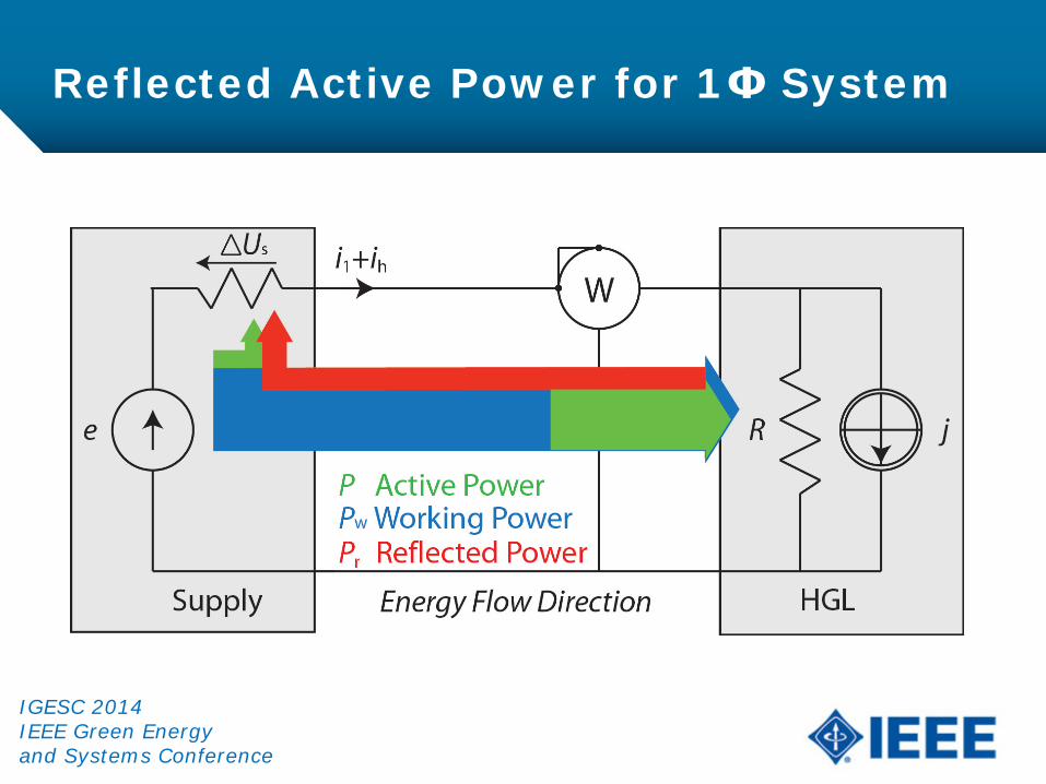
Reflected Active Power for 1Φ System
1Φ, sinusoidal voltage supply with purely resistive HGL.
Waveform distortion caused by non-linearity of the load can be modeled as a current source in the load.
Fundamental & higher harmonics
10
( ) ( ) ( ) ( )n hi t i t i t i t∞
= = +∑
10
( ) ( ) ( ) ( )n hu t u t u t u t∞
= = +∑
IGESC 2014 IEEE Green Energy and Systems Conference
Reflected Active Power for 1Φ System
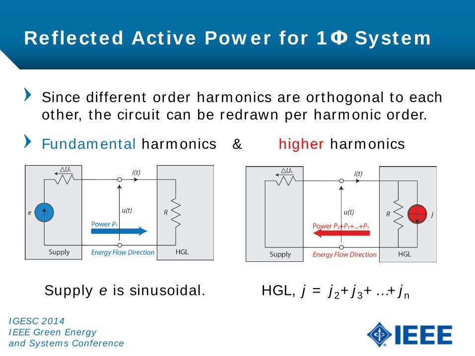
Since different order harmonics are orthogonal to each other, the circuit can be redrawn per harmonic order.
Fundamental harmonics & higher harmonics
Supply e is sinusoidal. HGL, j = j2+j3+…+jn
IGESC 2014 IEEE Green Energy and Systems Conference
Reflected Active Power for 1Φ System
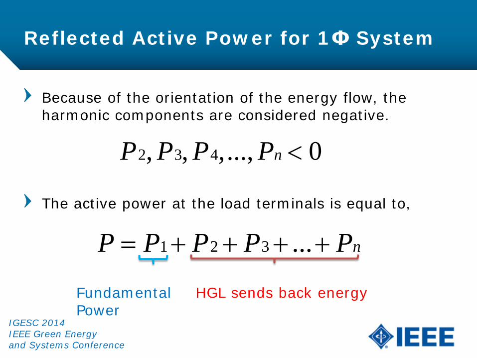
Because of the orientation of the energy flow, the harmonic components are considered negative.
The active power at the load terminals is equal to,
1 2 3 ... nP P P P P= + + + +
2 3 4, , ,..., 0nP P P P <
HGL sends back energy Fundamental Power
IGESC 2014 IEEE Green Energy and Systems Conference
Reflected Active Power for 1Φ System
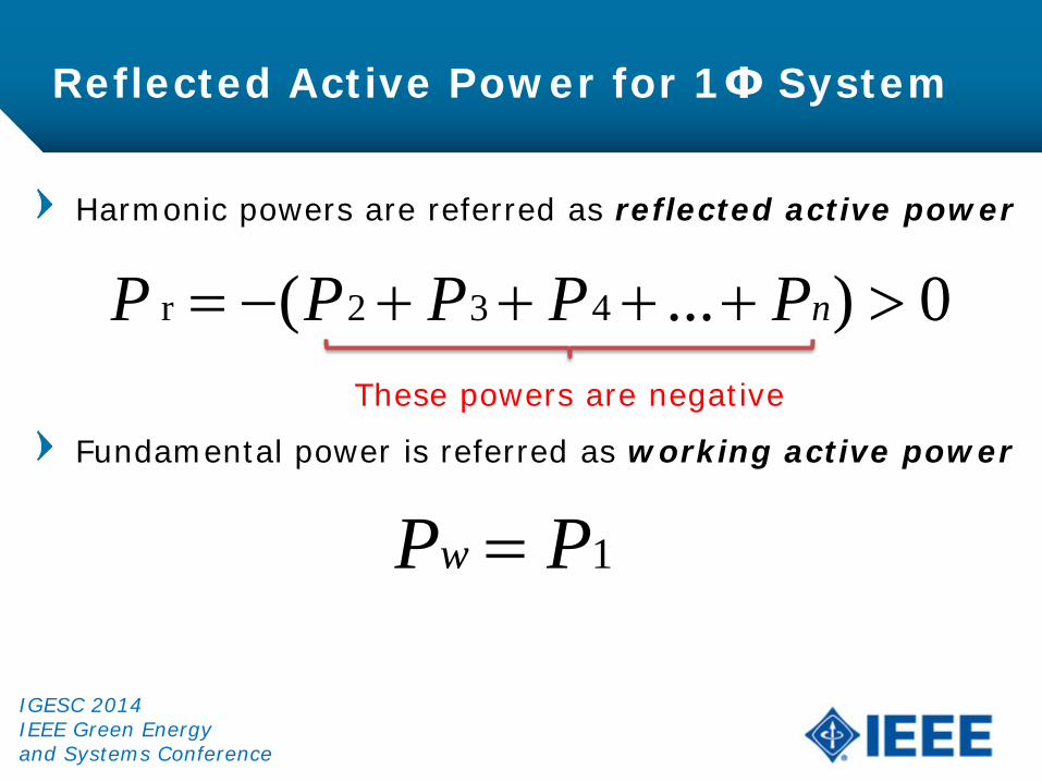
Harmonic powers are referred as reflected active power
Fundamental power is referred as working active power
r 2 3 4( ... ) 0nP P P P P= − + + + + >
1wP P=
These powers are negative
IGESC 2014 IEEE Green Energy and Systems Conference
Reflected Active Power for 1Φ System
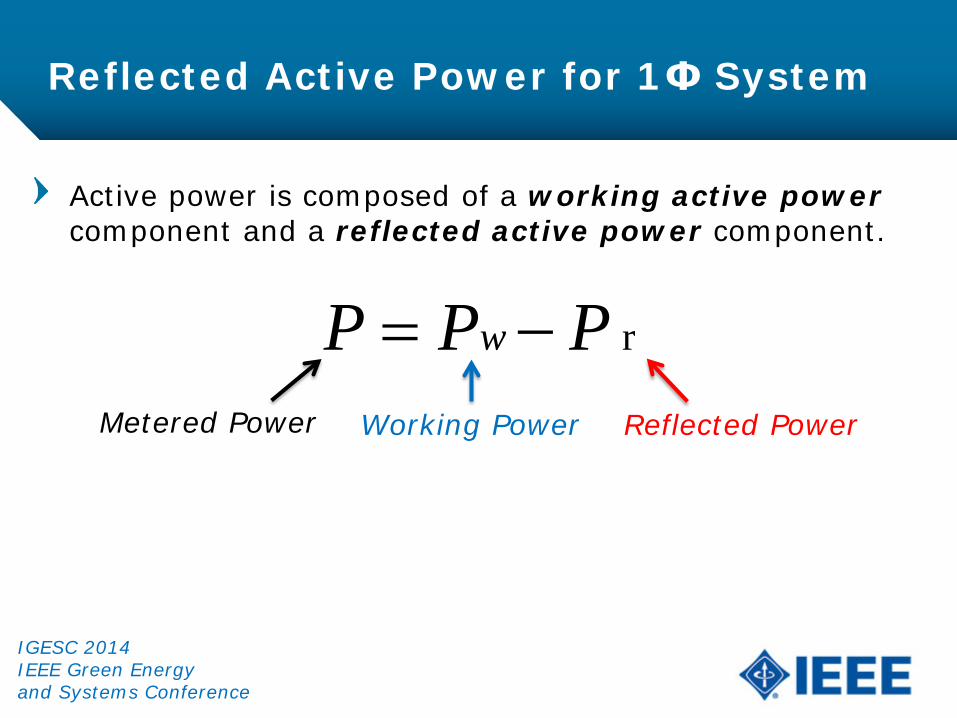
Active power is composed of a working active power component and a reflected active power component.
rwP P P= −Working Power Reflected Power Metered Power
IGESC 2014 IEEE Green Energy and Systems Conference
Reflected Active Power for 1Φ System
IGESC 2014 IEEE Green Energy and Systems Conference
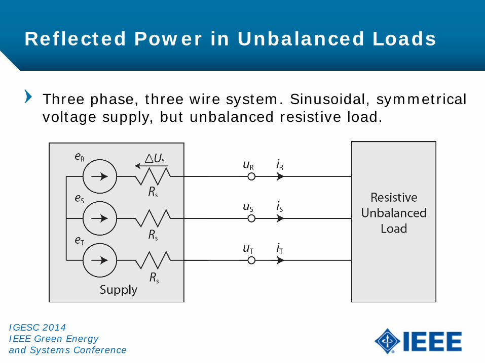
Reflected Power in Unbalanced Loads
Three phase, three wire system. Sinusoidal, symmetrical voltage supply, but unbalanced resistive load.
IGESC 2014 IEEE Green Energy and Systems Conference
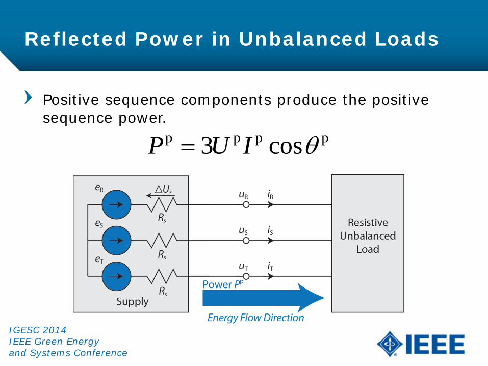
Reflected Power in Unbalanced Loads
Positive sequence components produce the positive sequence power.
p p p p3 cosP U I θ=
IGESC 2014 IEEE Green Energy and Systems Conference
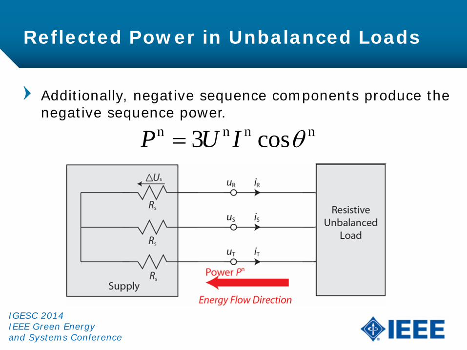
Reflected Power in Unbalanced Loads
Additionally, negative sequence components produce the negative sequence power.
n n n n3 cosP U I θ=
IGESC 2014 IEEE Green Energy and Systems Conference
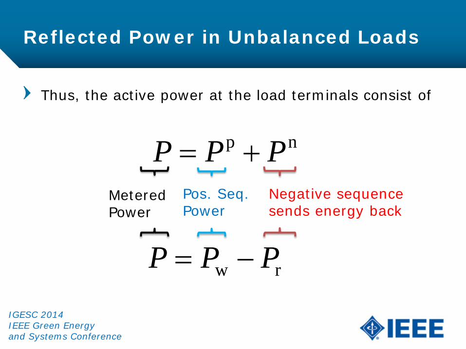
Reflected Power in Unbalanced Loads
Thus, the active power at the load terminals consist of
p nP P P= +Negative sequence sends energy back
Pos. Seq. Power
Metered Power
w rP P P= −
IGESC 2014 IEEE Green Energy and Systems Conference
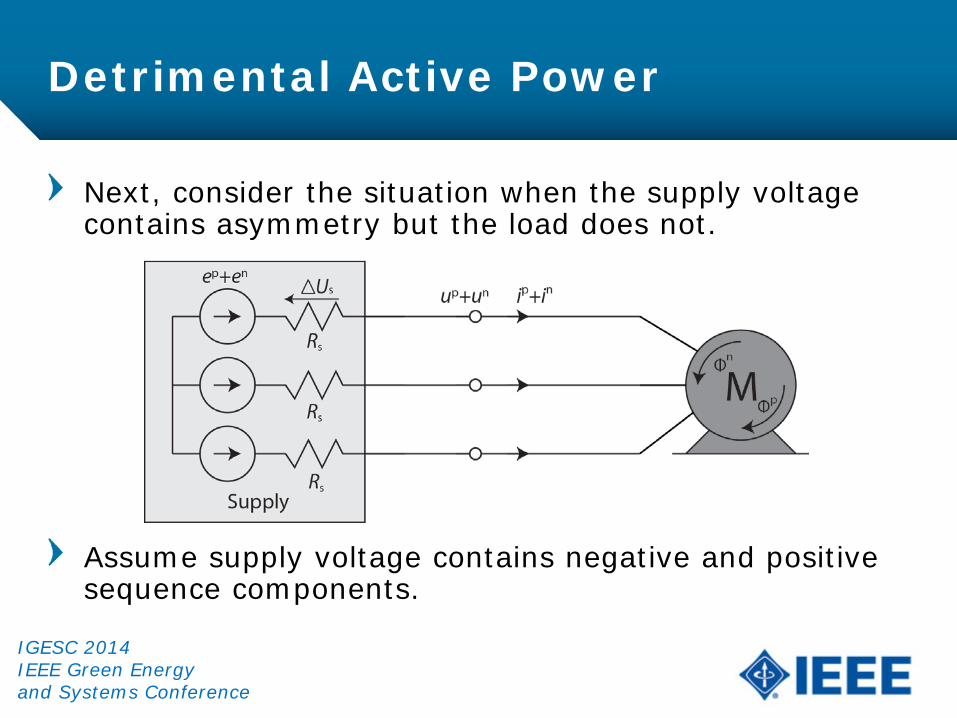
Detrimental Active Power
Next, consider the situation when the supply voltage contains asymmetry but the load does not.
Assume supply voltage contains negative and positive sequence components.
IGESC 2014 IEEE Green Energy and Systems Conference

Detrimental Active Power
In response to asymmetrical supply voltage, the motor current contains positive and negative sequence.
Thus, the active power at the motor terminals consist of,
p nP P P= +
Reduces motor torque Increases heat & wear
Converts to output power*
*Minus losses of the motor IGESC 2014 IEEE Green Energy and Systems Conference

Detrimental Active Power
Therefore, Pn should be regarded as detrimental active power,
And Pp should be regarded as working active power,
ndP P=
pwP P=
IGESC 2014 IEEE Green Energy and Systems Conference
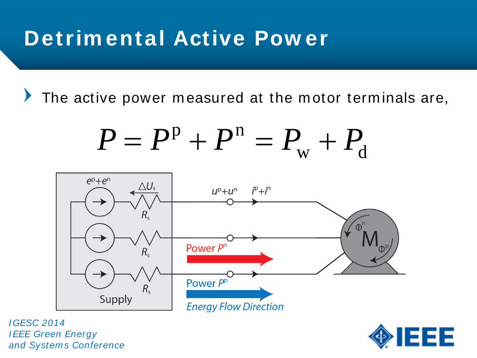
Detrimental Active Power
The active power measured at the motor terminals are,
p nw dP P P P P= + = +
IGESC 2014 IEEE Green Energy and Systems Conference

Detrimental Active Power
Supply voltage harmonics induces magnetic fields rotating at nth order speed that could harm the motor.
And the harmonic power can be regarded as detrimental
2 3 4h ... nP P P P P= + + + +
nd hP P P= +
IGESC 2014 IEEE Green Energy and Systems Conference
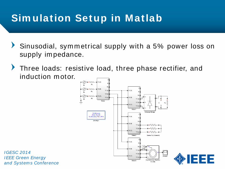
Sinusodial, symmetrical supply with a 5% power loss on supply impedance.
Three loads: resistive load, three phase rectifier, and induction motor.
Simulation Setup in Matlab
IGESC 2014 IEEE Green Energy and Systems Conference
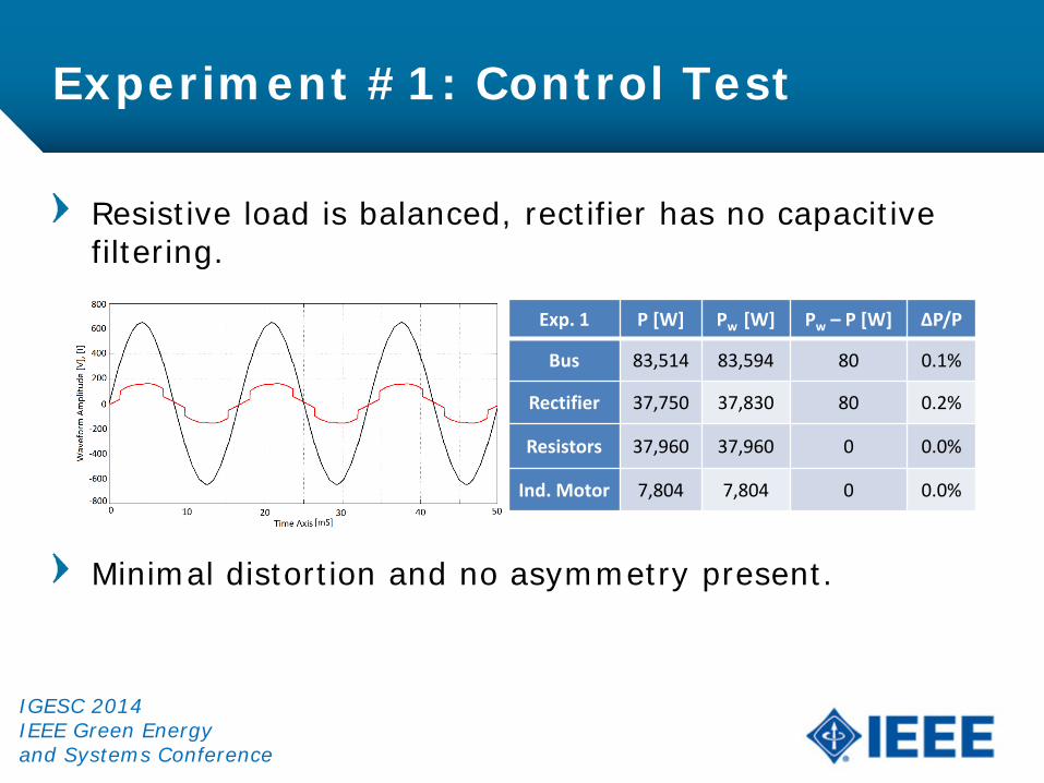
Resistive load is balanced, rectifier has no capacitive filtering.
Minimal distortion and no asymmetry present.
Experiment #1: Control Test
IGESC 2014 IEEE Green Energy and Systems Conference
Exp. 1 P [W] Pw [W] Pw – P [W] ∆P/P
Bus 83,514 83,594 80 0.1%
Rectifier 37,750 37,830 80 0.2%
Resistors 37,960 37,960 0 0.0%
Ind. Motor 7,804 7,804 0 0.0%

Resistive load is disconnected, rectifier has capacitive filter with 70% current THD and induction motor running
Rectifier causes reflected active power that results in an additional 2.2% power loss on the supply.
Exp. #2: Rectifier and Induction Motor
IGESC 2014 IEEE Green Energy and Systems Conference
Exp. 2 P [W] Pw [W] Pw – P [W] ∆P/P
Source 83,704 85,571 1,867 2.2%
Rectifier 75,380 77,250 1,870 2.5%
Ind. Motor 8324 8321 -3 0.04%
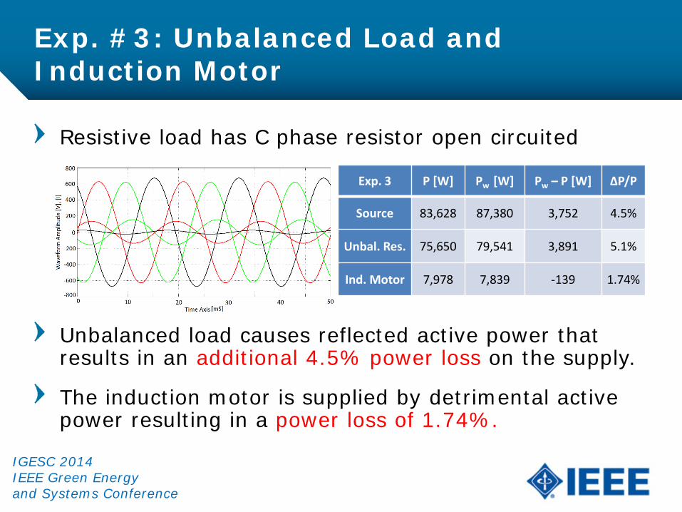
Resistive load has C phase resistor open circuited
Unbalanced load causes reflected active power that results in an additional 4.5% power loss on the supply.
The induction motor is supplied by detrimental active power resulting in a power loss of 1.74%.
Exp. #3: Unbalanced Load and Induction Motor
IGESC 2014 IEEE Green Energy and Systems Conference
Exp. 3 P [W] Pw [W] Pw – P [W] ∆P/P
Source 83,628 87,380 3,752 4.5%
Unbal. Res. 75,650 79,541 3,891 5.1%
Ind. Motor 7,978 7,839 -139 1.74%
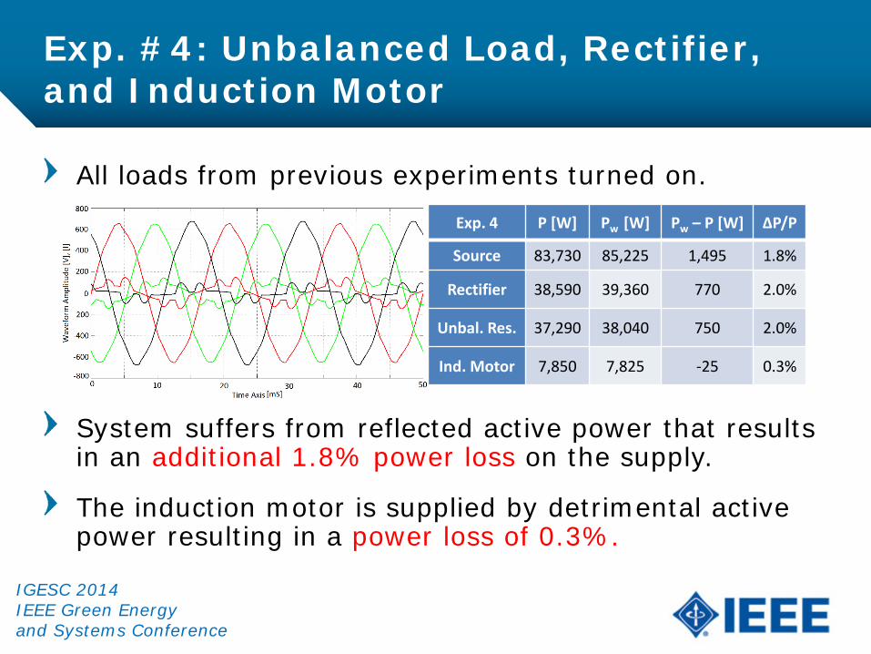
All loads from previous experiments turned on.
System suffers from reflected active power that results in an additional 1.8% power loss on the supply.
The induction motor is supplied by detrimental active power resulting in a power loss of 0.3%.
Exp. #4: Unbalanced Load, Rectifier, and Induction Motor
IGESC 2014 IEEE Green Energy and Systems Conference
Exp. 4 P [W] Pw [W] Pw – P [W] ∆P/P
Source 83,730 85,225 1,495 1.8%
Rectifier 38,590 39,360 770 2.0%
Unbal. Res. 37,290 38,040 750 2.0%
Ind. Motor 7,850 7,825 -25 0.3%

Sources of distortion (rectifier) and asymmetry (unbalanced load) caused a reflected active power component resulting in higher utility power loss.
Induction motor suffered detrimental active power from asymmetrical supply voltage the most. The voltage distortion affected the motor to a lesser extent. Overall, this causes power loss in the motor and overpayment of the customer.
Experimental Results
IGESC 2014 IEEE Green Energy and Systems Conference
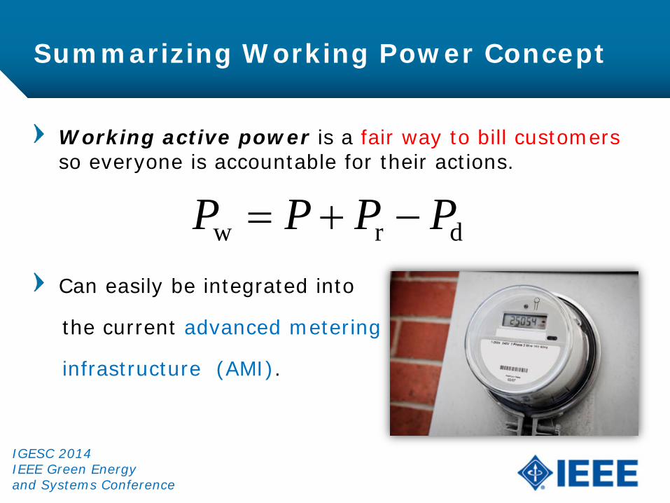
Working active power is a fair way to bill customers so everyone is accountable for their actions.
Can easily be integrated into
the current advanced metering
infrastructure (AMI).
w r dP P P P= + −
Summarizing Working Power Concept
IGESC 2014 IEEE Green Energy and Systems Conference

Conclusion
Working power concept accurately bills customers for their fair energy usage.
• Reflected active power refers to revenue loss of utility. (Penalize customer)
• Detrimental active power refers to customer overpayment. (Reimburse customer)
Using penalties, this will cause economic incentives to reduce overall distortion and asymmetry in the system.
Microgrids can benefit the most from the working power concept and can be easily integrated with AMI.
IGESC 2014 IEEE Green Energy and Systems Conference

Questions and Comments?
Are there any questions or comments?
Contact email: Tracy N. Toups: [email protected]
Leszek S. Czarnecki: [email protected]
Thank you for your attention and time.
IGESC 2014 IEEE Green Energy and Systems Conference
Elnaz Abdollahi, Haichao Wang, Samuli Rinne, Risto Lahdelma Department of Energy Technology [email protected] 24.11.2014
Optimization of energy production of a CHP plant with heat storage
This talk presents a linear programming (LP) model for a CHP plant with heat storage
2
• Demand for cheaper and
more efficient energy
production
• Combined heat and power
(CHP) optimization
• Computational results
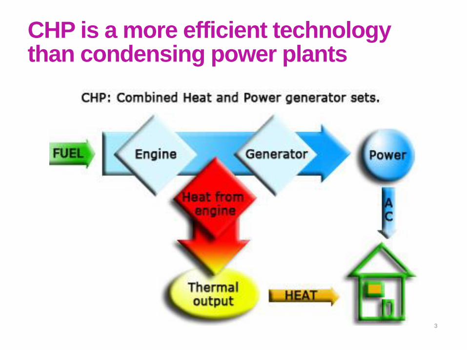
CHP is a more efficient technology than condensing power plants
3
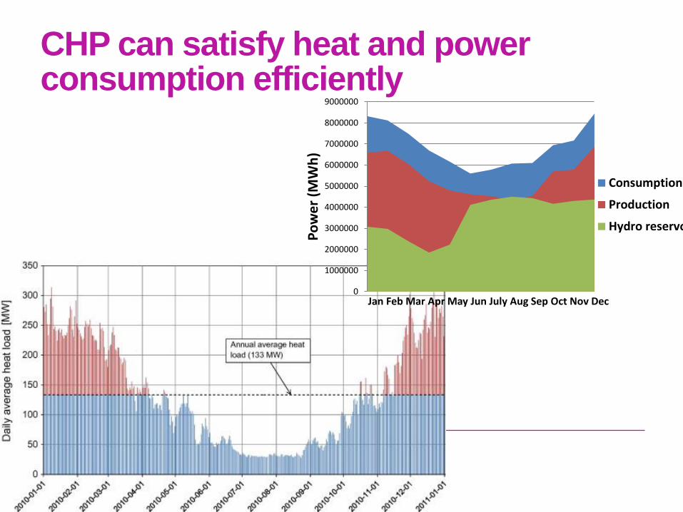
CHP can satisfy heat and power consumption efficiently
0
1000000
2000000
3000000
4000000
5000000
6000000
7000000
8000000
9000000
Po
we
r (M
Wh
) Jan Feb Mar Apr May Jun July Aug Sep Oct Nov Dec
Consumption
Production
Hydro reservoir
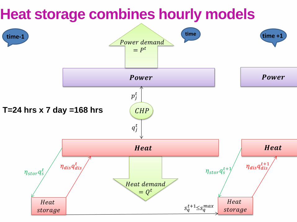
Heat storage combines hourly models
𝑷𝒐𝒘𝒆𝒓
𝐻𝑒𝑎𝑡 𝑠𝑡𝑜𝑟𝑎𝑔𝑒
𝐻𝑒𝑎𝑡 𝑑𝑒𝑚𝑎𝑛𝑑= 𝑄𝑡
𝑯𝒆𝒂𝒕
𝑷𝒐𝒘𝒆𝒓
𝑯𝒆𝒂𝒕
𝑃𝑜𝑤𝑒𝑟 𝑑𝑒𝑚𝑎𝑛𝑑= 𝑃𝑡
𝐻𝑒𝑎𝑡 𝑠𝑡𝑜𝑟𝑎𝑔𝑒
𝜂𝑑𝑖𝑠𝑞𝑑𝑖𝑠𝑡
𝜂𝑠𝑡𝑜𝑟𝑞𝑠𝑡
𝐶𝐻𝑃
𝑞𝑗𝑡
𝑝𝑗𝑡
𝑠𝑞𝑡+1𝑠𝑞
𝑚𝑎𝑥
𝜂𝑑𝑖𝑠𝑞𝑑𝑖𝑠𝑡+1
𝜂𝑠𝑡𝑜𝑟𝑞𝑠𝑡+1
time-1 time time +1
T=24 hrs x 7 day =168 hrs

Convexity assumption
6
• We assume the CHP plant model is convex: • the operating region is convex
• the objective function to minimize is convex
• A set X is convex if the line segment connecting any two points x and y of the set is in the set
• Mathematically
– If x,yX, then x+(1- )yX for all [0,1]
x
y
X is convex
x y
X is non-convex
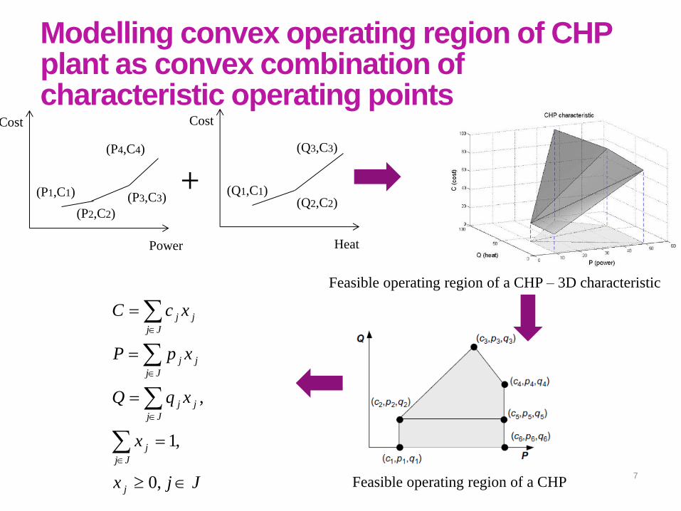
Modelling convex operating region of CHP plant as convex combination of characteristic operating points
7
Power
Cost
(P1,C1)
(P2,C2)
(P3,C3)
(P4,C4)
Heat
Cost
(Q1,C1) (Q2,C2)
(Q3,C3)
Feasible operating region of a CHP
Feasible operating region of a CHP – 3D characteristic
Jjx
x
xqQ
xpP
xcC
j
Jj
j
j
Jj
j
j
Jj
j
j
Jj
j
,0
,1
,
+
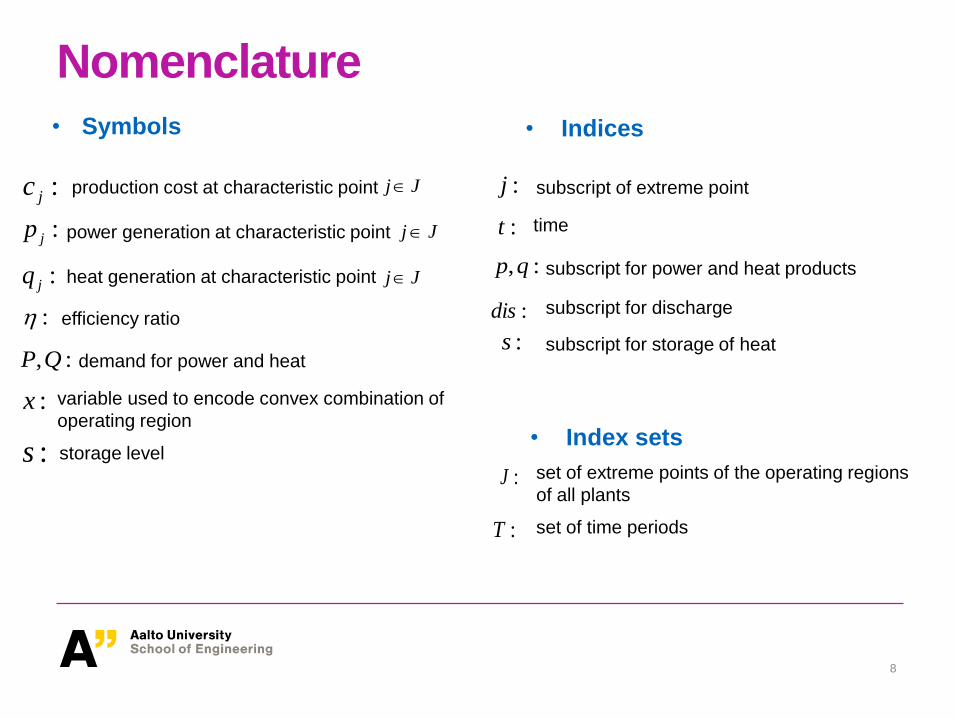
Nomenclature
8
production cost at characteristic point
power generation at characteristic point
heat generation at characteristic point
:jc
:jp
:jq
: efficiency ratio
:,QP demand for power and heat
• Indices
:x variable used to encode convex combination of
operating region
• Symbols
:j subscript of extreme point
:s storage level
:t time
:,qp subscript for power and heat products
:dis subscript for discharge
:s subscript for storage of heat
• Index sets
:J set of extreme points of the operating regions
of all plants
:T set of time periods
Jj
Jj
Jj
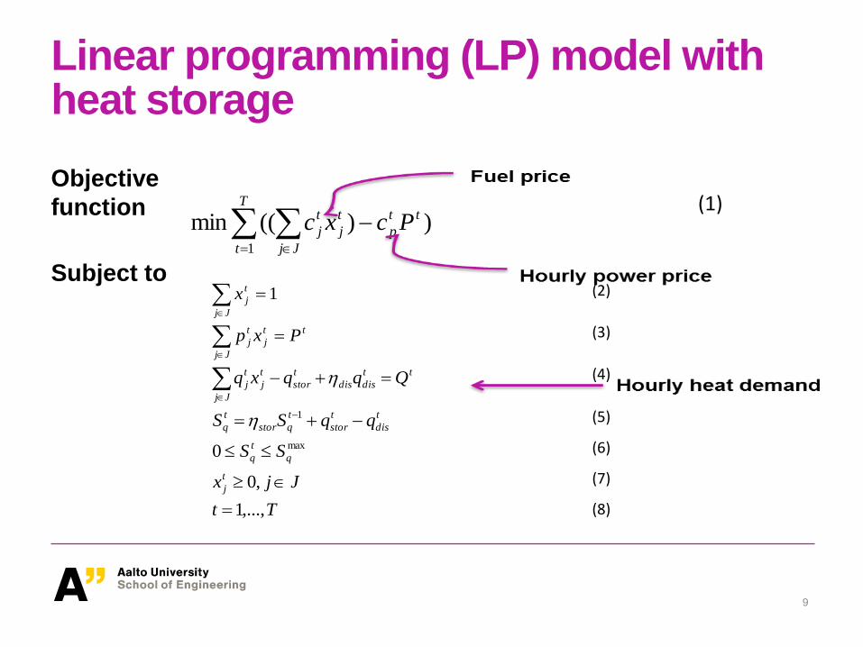
Linear programming (LP) model with heat storage
9
))((min1
tt
p
t
j
T
t Jj
t
j Pcxc
(1)
Objective
function
Subject to 1
Jj
t
jx
(2)
t
Jj
t
j
t
j Pxp
(3)
tt
disdis
t
stor
t
j
Jj
t
j Qqqxq
(4)
t
dis
t
stor
t
qstor
t
q qqSS 1 (5)
max0 q
t
q SS (6)
Jjxt
j ,0 (7)
Tt ,...,1 (8)
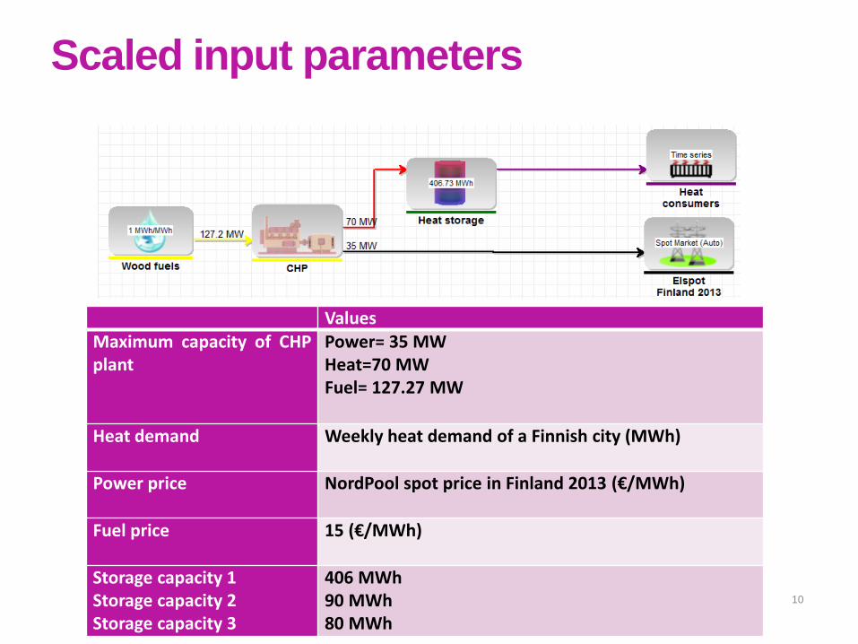
Scaled input parameters
10
Values Maximum capacity of CHP plant
Power= 35 MW Heat=70 MW Fuel= 127.27 MW
Heat demand Weekly heat demand of a Finnish city (MWh)
Power price NordPool spot price in Finland 2013 (€/MWh)
Fuel price 15 (€/MWh)
Storage capacity 1 Storage capacity 2 Storage capacity 3
406 MWh 90 MWh 80 MWh
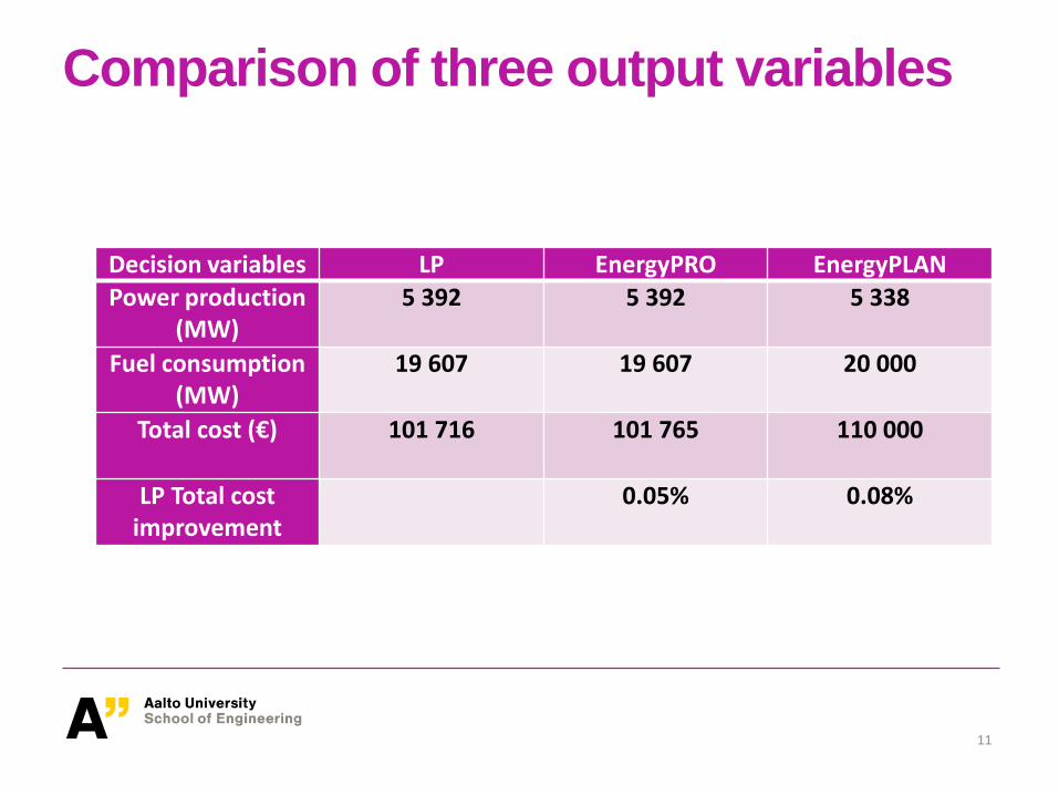
Comparison of three output variables
11
Decision variables LP EnergyPRO EnergyPLAN Power production
(MW) 5 392 5 392 5 338
Fuel consumption (MW)
19 607 19 607 20 000
Total cost (€) 101 716
101 765 110 000
LP Total cost improvement
0.05%
0.08%
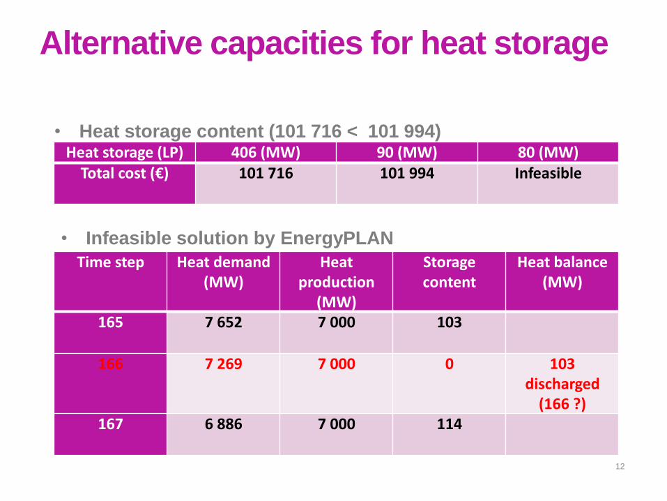
Alternative capacities for heat storage
12
• Heat storage content (101 716 < 101 994)
Time step Heat demand (MW)
Heat production
(MW)
Storage content
Heat balance (MW)
165 7 652 7 000 103
166 7 269 7 000 0 103 discharged
(166 ?) 167 6 886
7 000 114
Heat storage (LP) 406 (MW) 90 (MW) 80 (MW) Total cost (€)
101 716
101 994 Infeasible
• Infeasible solution by EnergyPLAN
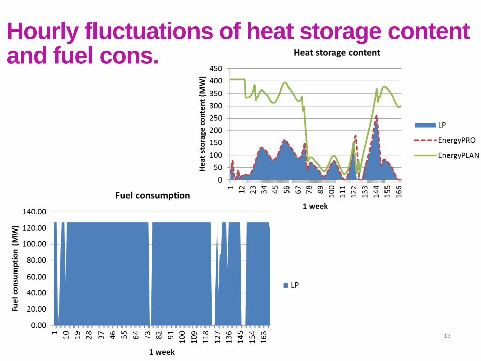
Hourly fluctuations of heat storage content and fuel cons.
13

Towards more efficient and clean energy • The proposed model can optimize the CHP with high
flexibility.
• Large-scale energy production models should also be
developed to facilitate more economic energy production.
14

SNR Estimation and Jamming Detection Techniques Using Wavelets
Green Energy and Systems Conference 2014
By: Paula Quintana California State University, Long Beach
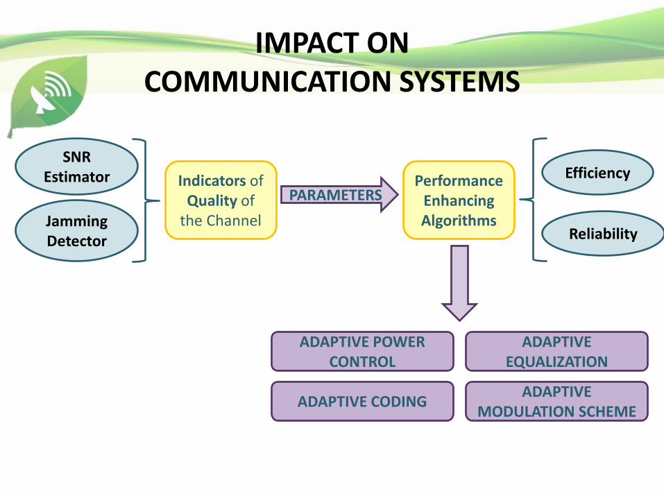
IMPACT ON
COMMUNICATION SYSTEMS
SNR Estimator
Jamming Detector
Indicators of Quality of
the Channel
PARAMETERS Performance
Enhancing Algorithms
Efficiency
Reliability
ADAPTIVE POWER CONTROL
ADAPTIVE EQUALIZATION
ADAPTIVE CODING ADAPTIVE
MODULATION SCHEME
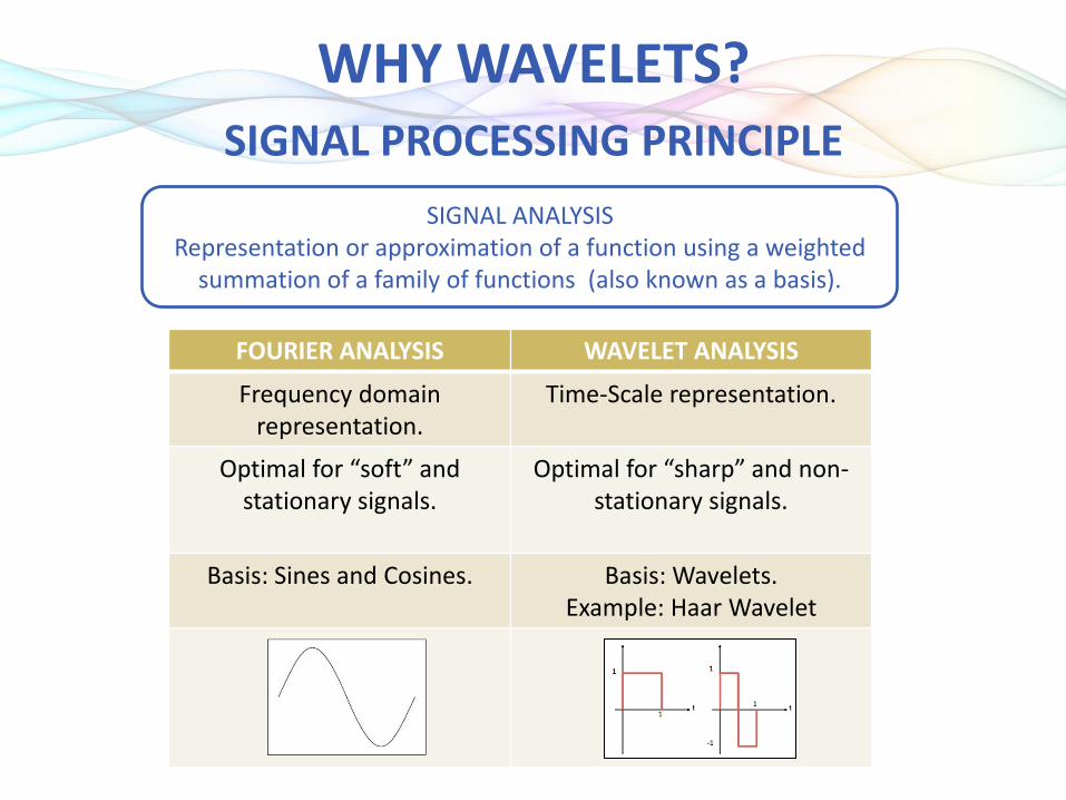
WHY WAVELETS? SIGNAL PROCESSING PRINCIPLE
SIGNAL ANALYSIS Representation or approximation of a function using a weighted
summation of a family of functions (also known as a basis).
FOURIER ANALYSIS WAVELET ANALYSIS
Frequency domain representation.
Time-Scale representation.
Optimal for “soft” and stationary signals.
Optimal for “sharp” and non-stationary signals.
Basis: Sines and Cosines. Basis: Wavelets. Example: Haar Wavelet
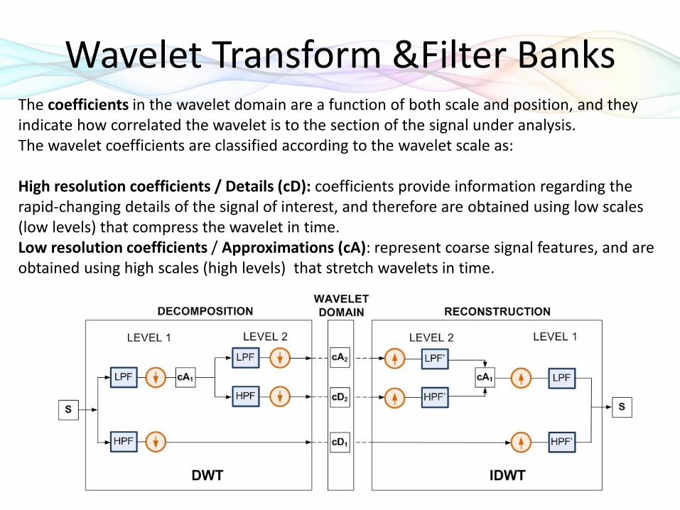
Wavelet Transform &Filter Banks The coefficients in the wavelet domain are a function of both scale and position, and they indicate how correlated the wavelet is to the section of the signal under analysis. The wavelet coefficients are classified according to the wavelet scale as: High resolution coefficients / Details (cD): coefficients provide information regarding the rapid-changing details of the signal of interest, and therefore are obtained using low scales (low levels) that compress the wavelet in time. Low resolution coefficients / Approximations (cA): represent coarse signal features, and are obtained using high scales (high levels) that stretch wavelets in time.
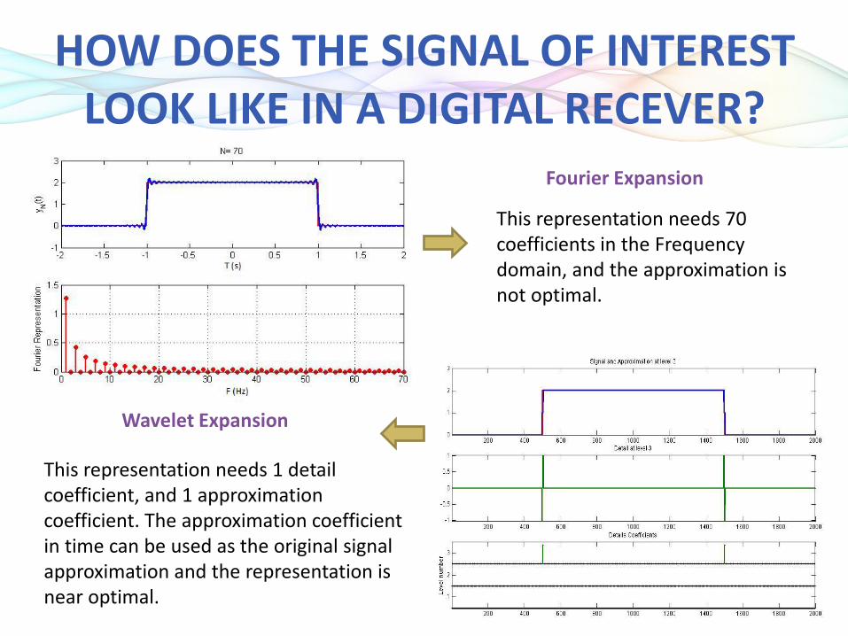
HOW DOES THE SIGNAL OF INTEREST LOOK LIKE IN A DIGITAL RECEVER?
Fourier Expansion
This representation needs 70 coefficients in the Frequency domain, and the approximation is not optimal.
Wavelet Expansion
This representation needs 1 detail coefficient, and 1 approximation coefficient. The approximation coefficient in time can be used as the original signal approximation and the representation is near optimal.
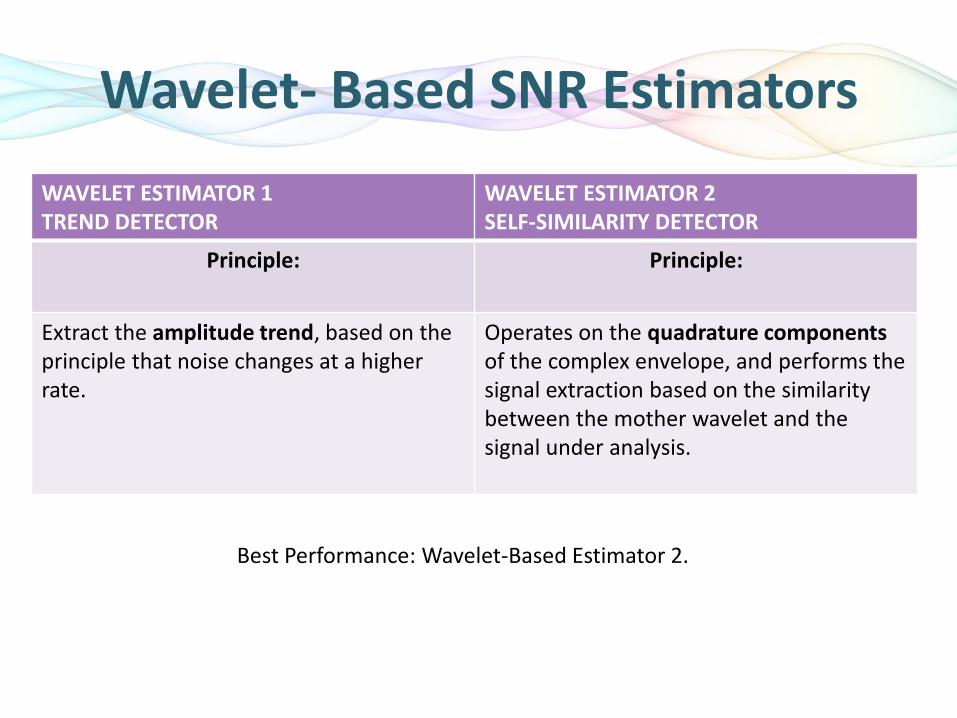
Wavelet- Based SNR Estimators
WAVELET ESTIMATOR 1 TREND DETECTOR
WAVELET ESTIMATOR 2 SELF-SIMILARITY DETECTOR
Principle:
Principle:
Extract the amplitude trend, based on the principle that noise changes at a higher rate.
Operates on the quadrature components of the complex envelope, and performs the signal extraction based on the similarity between the mother wavelet and the signal under analysis.
Best Performance: Wavelet-Based Estimator 2.
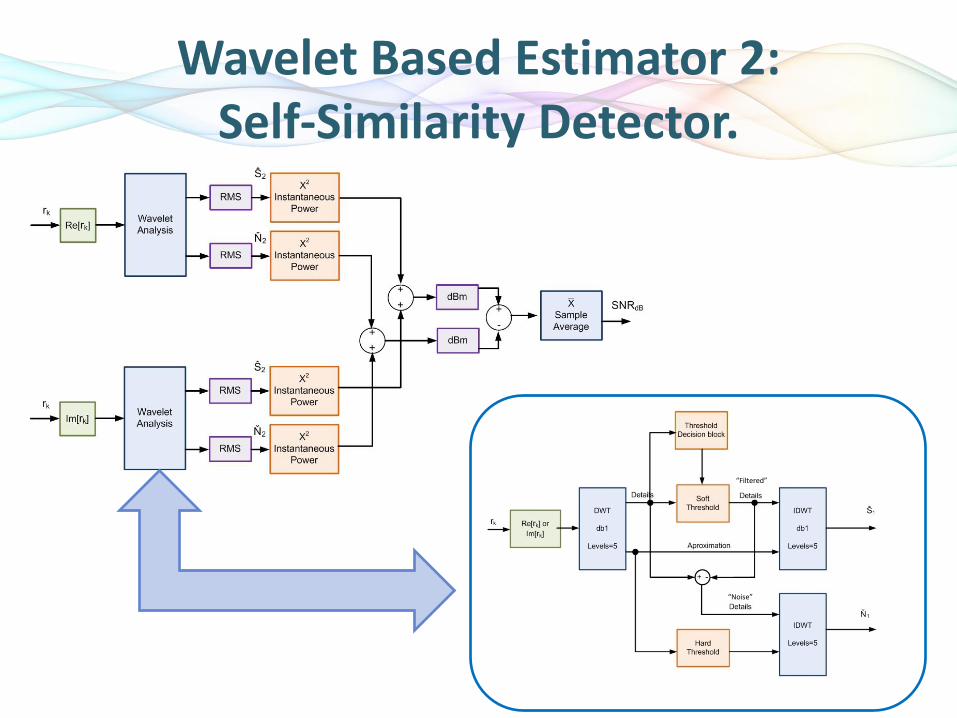
Wavelet Based Estimator 2: Self-Similarity Detector.
“Filtered”
“Noise”
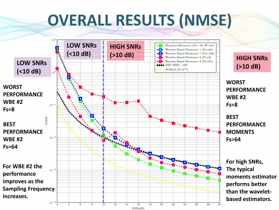
OVERALL RESULTS (NMSE)
LOW SNRs (<10 dB)
BEST PERFORMANCE WBE #2 Fs=64
WORST PERFORMANCE WBE #2 Fs=8
LOW SNRs (<10 dB)
For WBE #2 the performance improves as the Sampling Frequency increases.
HIGH SNRs (>10 dB) HIGH SNRs
(>10 dB)
WORST PERFORMANCE WBE #2 Fs=8
BEST PERFORMANCE MOMENTS Fs=64
For high SNRs, The typical moments estimator performs better than the wavelet-based estimators.

OVERALL RESULTS (NBIAS) LOW SNRs (<10 dB)
LOW SNRs (<10 dB)
BEST PERFORMANCE WBE #2 -Fs=64 -Fs=8
WORST PERFORMANCE -WBE #1 Fs=64 -MOMENTS
WBE #2 DISPLAYS THE LOWEST BIAS, (EVEN FOR LOW Fs).
HIGH SNRs (>10 dB)
WORST PERFORMANCE -WBE #2 Fs=8
BEST PERFORMANCE -WBE #2 Fs=64 -MOMENTS For WBE #2 the performance improves as the Sampling Frequency increases.
HIGH SNRs (>10 dB)
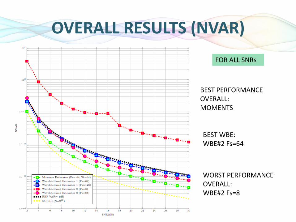
OVERALL RESULTS (NVAR)
FOR ALL SNRs
BEST PERFORMANCE OVERALL: MOMENTS
BEST WBE: WBE#2 Fs=64
WORST PERFORMANCE OVERALL: WBE#2 Fs=8
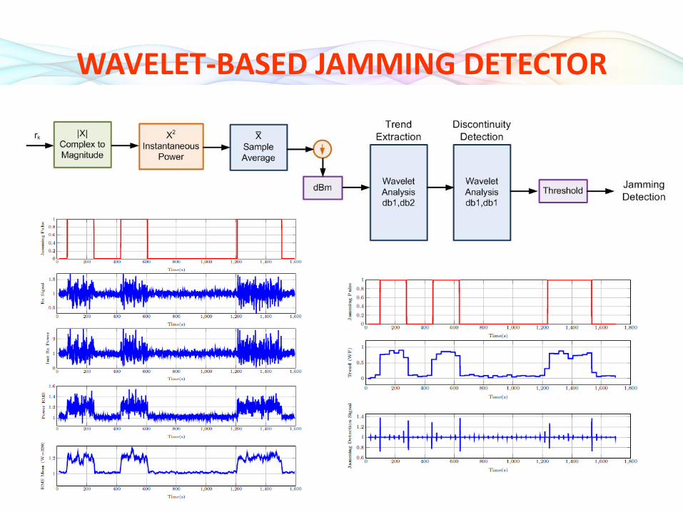
WAVELET-BASED JAMMING DETECTOR
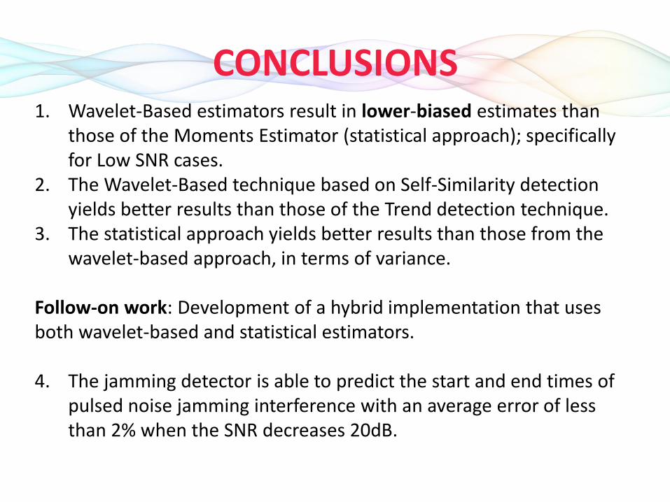
CONCLUSIONS 1. Wavelet-Based estimators result in lower-biased estimates than
those of the Moments Estimator (statistical approach); specifically for Low SNR cases.
2. The Wavelet-Based technique based on Self-Similarity detection yields better results than those of the Trend detection technique.
3. The statistical approach yields better results than those from the wavelet-based approach, in terms of variance.
Follow-on work: Development of a hybrid implementation that uses both wavelet-based and statistical estimators. 4. The jamming detector is able to predict the start and end times of
pulsed noise jamming interference with an average error of less than 2% when the SNR decreases 20dB.

THANK YOU!
QUESTIONS?

Richard Lam
Henry Yeh
PV Ramp Limiting with Adaptive Smoothing through
a Battery Energy Storage System (BESS)

•Solar PV Issues
•BESS Diagram
•PV Smoothing
•Adaptive Smoothing
•Ramp Limiting
Overview
•Ramp Limiting & PV Smoothing
•Real World Cases and performance results

• Solar Photovoltaics (PV) is a variable generation• The sun doesn’t always shine!
• Power is dependent on Weather• Cloudy days cause issues
• Solar irradiance can rise and fall rapidly
• Issues with high ramp rates• Can cause voltage rapid voltage fluctuations
• System frequency may become unstable
• High PV penetration is a real issue• CA requires 33% renewables by 2020
• 50% by 2030 may be possible
• Areas with High PV penetration would benefit most• Microgrids such as Lanai island in Hawaii
• Not yet necessary on larger grids…
The Issue With Solar Variability

Issue With Solar Variability Contd.
• 𝑅𝑅𝐴𝑇𝐸𝑃𝑉 𝑡 =𝑃𝑃𝑉 𝑡 −𝑃𝑃𝑉 𝑡−1
∆𝑡
• KEMA study shows 3.6 MW/min was the limit for the Lanai 1.2 MW array
• 20% PV Penetration
• Higher ramp rates can cause inverters to trip off -IEEE 1547 Limit
• Grid frequency limits almost exceeded despite local diesel generators providing support
• 1.2 MW PV Array reduced to 600 kW output to limit risk.
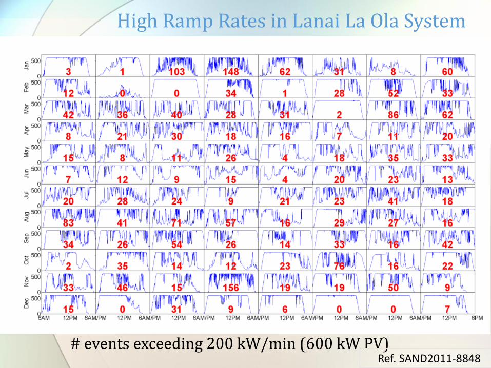
High Ramp Rates in Lanai La Ola System
# events exceeding 200 kW/min (600 kW PV)Ref. SAND2011-8848
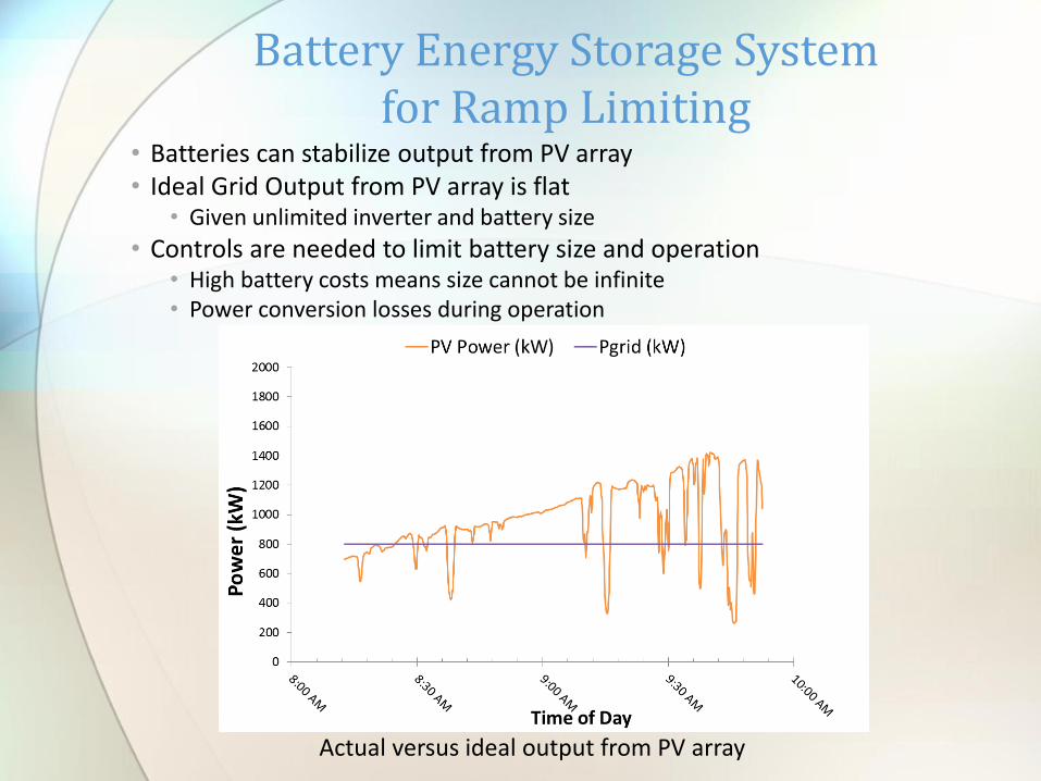
• Batteries can stabilize output from PV array• Ideal Grid Output from PV array is flat
• Given unlimited inverter and battery size
• Controls are needed to limit battery size and operation• High battery costs means size cannot be infinite• Power conversion losses during operation
Battery Energy Storage System for Ramp Limiting
Actual versus ideal output from PV array
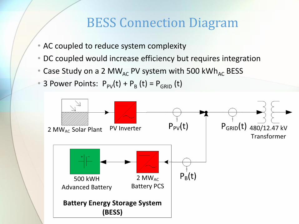
• AC coupled to reduce system complexity
• DC coupled would increase efficiency but requires integration
• Case Study on a 2 MWAC PV system with 500 kWhAC BESS
• 3 Power Points: PPV(t) + PB (t) = PGRID (t)
BESS Connection Diagram
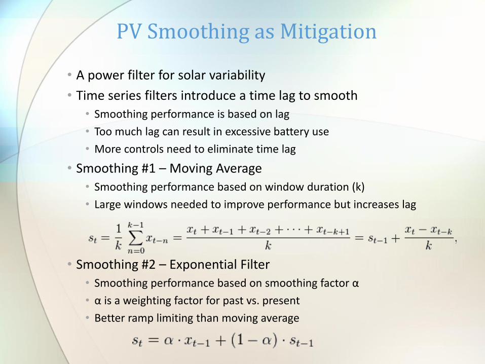
PV Smoothing as Mitigation
• A power filter for solar variability
• Time series filters introduce a time lag to smooth
• Smoothing performance is based on lag
• Too much lag can result in excessive battery use
• More controls need to eliminate time lag
• Smoothing #1 – Moving Average
• Smoothing performance based on window duration (k)
• Large windows needed to improve performance but increases lag
• Smoothing #2 – Exponential Filter
• Smoothing performance based on smoothing factor α
• α is a weighting factor for past vs. present
• Better ramp limiting than moving average
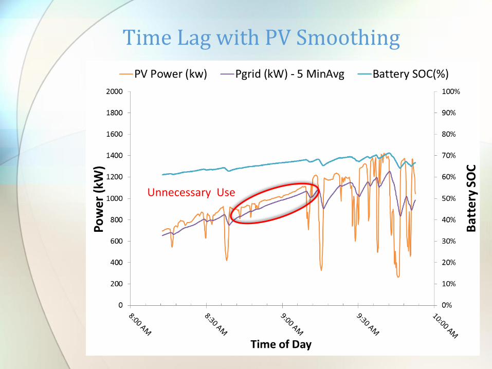
Time Lag with PV Smoothing
Unnecessary Use
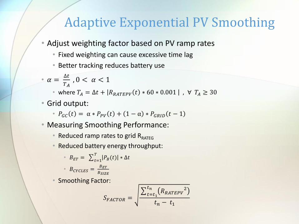
• Adjust weighting factor based on PV ramp rates
• Fixed weighting can cause excessive time lag
• Better tracking reduces battery use
• 𝛼 =∆𝑡
𝑇𝐴, 0 < 𝛼 < 1
• where 𝑇𝐴 = ∆𝑡 + 𝑅𝑅𝐴𝑇𝐸𝑃𝑉 𝑡 ∗ 60 ∗ 0.001 , ∀ 𝑇𝐴 ≥ 30
• Grid output: • 𝑃𝐺𝐶 𝑡 = α ∗ 𝑃𝑃𝑉 𝑡 + 1 − α ∗ 𝑃𝐺𝑅𝐼𝐷 𝑡 − 1
• Measuring Smoothing Performance:
• Reduced ramp rates to grid RRATEG
• Reduced battery energy throughput:
• 𝐵𝐸𝑇 = 𝑡=1𝑇𝑃𝐵(𝑡) ∗ ∆𝑡
• 𝐵𝐶𝑌𝐶𝐿𝐸𝑆 =𝐵𝐸𝑇
𝐵𝑆𝐼𝑍𝐸
• Smoothing Factor:
𝑆𝐹𝐴𝐶𝑇𝑂𝑅 = 𝑡=𝑡1
𝑡𝑛 𝑅𝑅𝐴𝑇𝐸𝑃𝑉2
𝑡𝑛 − 𝑡1
Adaptive Exponential PV Smoothing
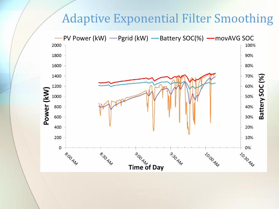
Adaptive Exponential Filter Smoothing

Ramp Limiting as Mitigation
• Fixed Time Window Ramp Limit (FTWRL)• Output based on average output
from previous 15 minutes (or longer)
• Excessive battery use but method has been used in other systems
• Variable Time Window Ramp Limit (VTWRL)• Limit ramp rates using PV ramp rate as a trigger
• Programmable Ramp Limit
• Only utilize BESS when PV ramp rates are high
• Significant reduction on battery use BET
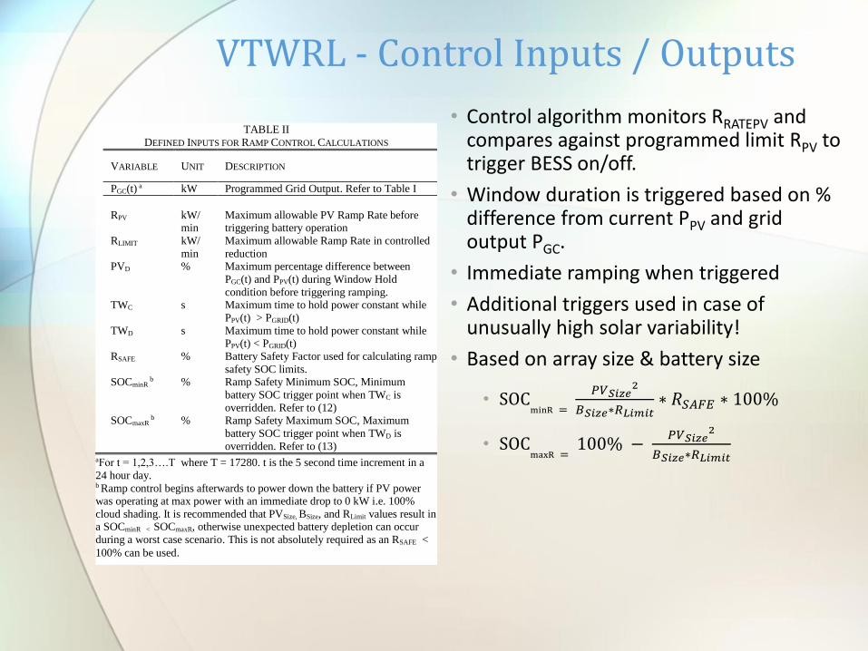
VTWRL - Control Inputs / Outputs
TABLE II
DEFINED INPUTS FOR RAMP CONTROL CALCULATIONS
VARIABLE UNIT DESCRIPTION
PGC(t) a kW Programmed Grid Output. Refer to Table I
RPV kW/
min
Maximum allowable PV Ramp Rate before
triggering battery operation
RLIMIT kW/
min
Maximum allowable Ramp Rate in controlled
reduction PVD % Maximum percentage difference between
PGC(t) and PPV(t) during Window Hold
condition before triggering ramping.
TWC s Maximum time to hold power constant while
PPV(t) > PGRID(t)
TWD s Maximum time to hold power constant while PPV(t) < PGRID(t)
RSAFE % Battery Safety Factor used for calculating ramp
safety SOC limits. SOCminR
b % Ramp Safety Minimum SOC, Minimum
battery SOC trigger point when TWC is
overridden. Refer to (12) SOCmaxR
b % Ramp Safety Maximum SOC, Maximum
battery SOC trigger point when TWD is
overridden. Refer to (13) aFor t = 1,2,3….T where T = 17280. t is the 5 second time increment in a
24 hour day. b Ramp control begins afterwards to power down the battery if PV power
was operating at max power with an immediate drop to 0 kW i.e. 100%
cloud shading. It is recommended that PVSize, BSize, and RLimit values result in a SOCminR < SOCmaxR, otherwise unexpected battery depletion can occur
during a worst case scenario. This is not absolutely required as an RSAFE <
100% can be used.
• Control algorithm monitors RRATEPV and compares against programmed limit RPV to trigger BESS on/off.
• Window duration is triggered based on % difference from current PPV and grid output PGC.
• Immediate ramping when triggered
• Additional triggers used in case of unusually high solar variability!
• Based on array size & battery size
• SOCminR =
𝑃𝑉𝑆𝑖𝑧𝑒2
𝐵𝑆𝑖𝑧𝑒∗𝑅𝐿𝑖𝑚𝑖𝑡∗ 𝑅𝑆𝐴𝐹𝐸 ∗ 100%
• SOCmaxR =
100% −𝑃𝑉𝑆𝑖𝑧𝑒
2
𝐵𝑆𝑖𝑧𝑒∗𝑅𝐿𝑖𝑚𝑖𝑡
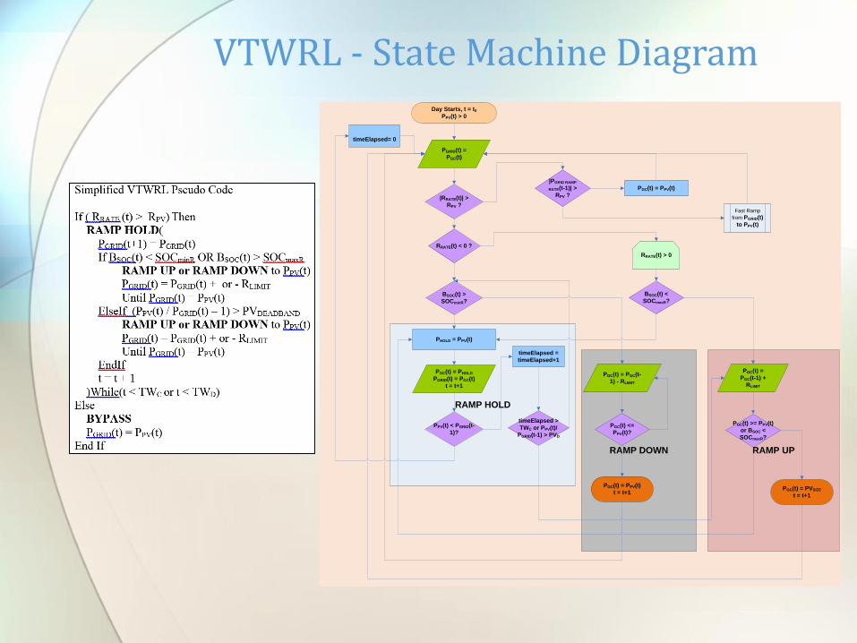
VTWRL - State Machine Diagram
RAMP HOLD
RAMP DOWN RAMP UP
|RRATE(t)| >
RPV ?
RRATE(t) < 0 ?
BSOC(t) >
SOCminR?
PHOLD = PPV(t)
Day Starts, t = t0
PPV(t) > 0
PGC(t) = PHOLD
PGRID(t) = PGC(t)
t = t+1
PGC(t) <=
PPV(t)?
PGRID(t) =
PGC(t)
RRATE(t) > 0
PGC(t) = PGC(t-
1) - RLIMIT
PGC(t) =
PGC(t-1) +
RLIMIT
BSOC(t) <
SOCmaxR?
PGC(t) = PPV(t)
timeElapsed= 0
PPV(t) < PGRID(t-
1)?
timeElapsed =
timeElapsed+1
timeElapsed >
TWC or PPV(t)/
PGRID(t-1) > PVD
PGC(t) >= PPV(t)
or BSOC <
SOCmaxR?
PGC(t) = PPV(t)
t = t+1PGC(t) = PVSIZE
t = t+1
|PGRID RAMP
RATE(t-1)| >
RPV ?
Fast Ramp
from PGRID(t)
to PPV(t)
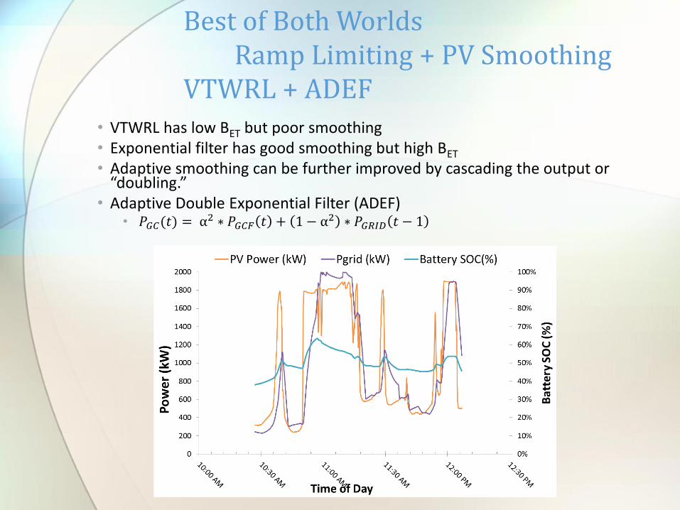
• VTWRL has low BET but poor smoothing• Exponential filter has good smoothing but high BET
• Adaptive smoothing can be further improved by cascading the output or “doubling.”
• Adaptive Double Exponential Filter (ADEF)• 𝑃𝐺𝐶(𝑡) = α
2 ∗ 𝑃𝐺𝐶𝐹 𝑡 + 1 − α2 ∗ 𝑃𝐺𝑅𝐼𝐷 𝑡 − 1
Best of Both Worlds Ramp Limiting + PV Smoothing
VTWRL + ADEF
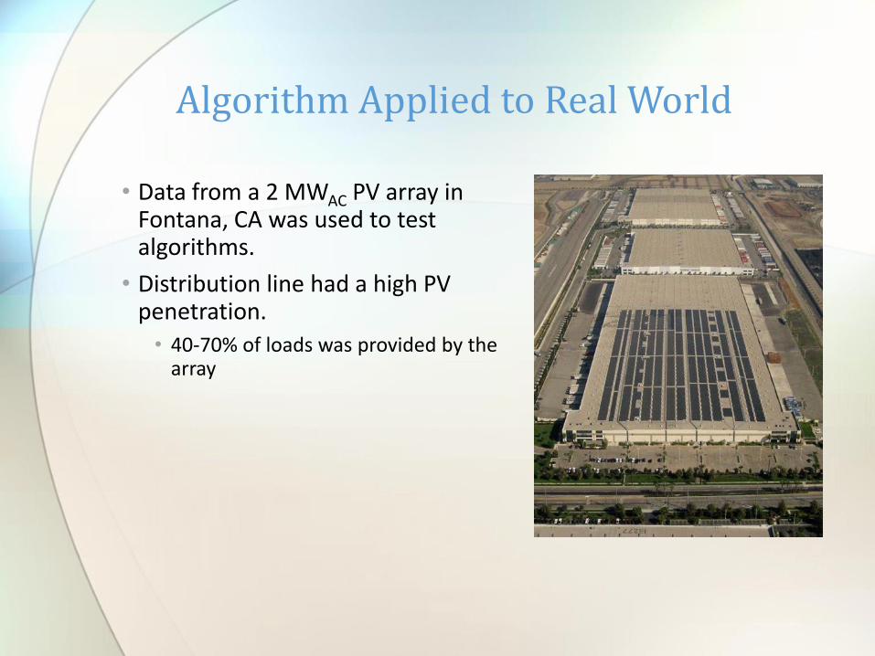
• Data from a 2 MWAC PV array in Fontana, CA was used to test algorithms.
• Distribution line had a high PV penetration.
• 40-70% of loads was provided by the array
Algorithm Applied to Real World
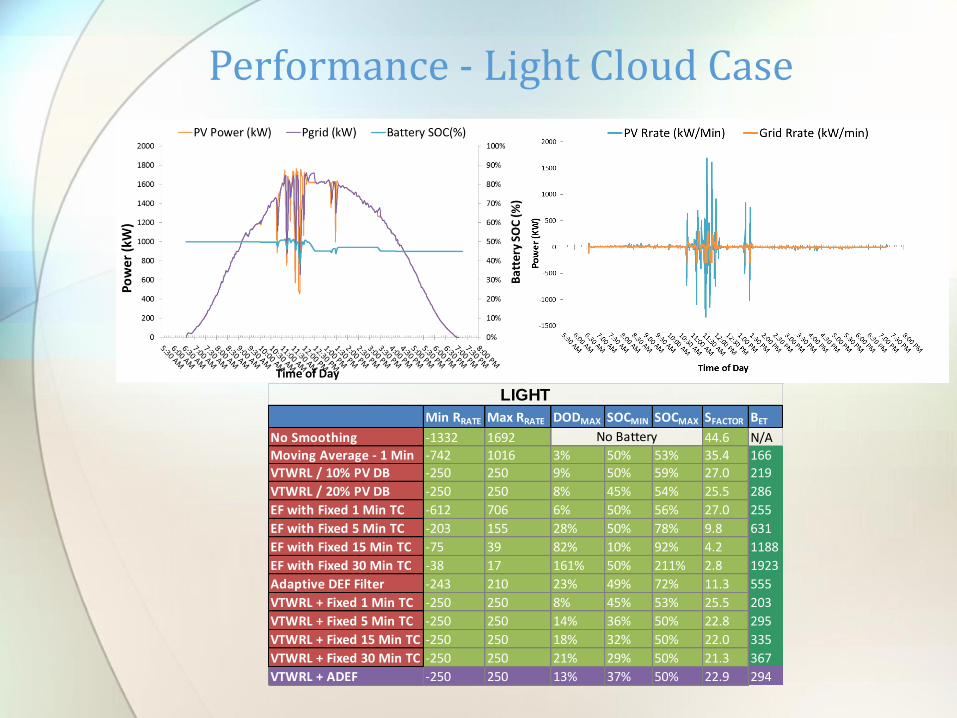
Performance - Light Cloud Case
Min RRATE Max RRATE DODMAX SOCMIN SOCMAX SFACTOR BET
No Smoothing -1332 1692 44.6 N/A
Moving Average - 1 Min -742 1016 3% 50% 53% 35.4 166VTWRL / 10% PV DB -250 250 9% 50% 59% 27.0 219
VTWRL / 20% PV DB -250 250 8% 45% 54% 25.5 286
EF with Fixed 1 Min TC -612 706 6% 50% 56% 27.0 255
EF with Fixed 5 Min TC -203 155 28% 50% 78% 9.8 631
EF with Fixed 15 Min TC -75 39 82% 10% 92% 4.2 1188
EF with Fixed 30 Min TC -38 17 161% 50% 211% 2.8 1923
Adaptive DEF Filter -243 210 23% 49% 72% 11.3 555
VTWRL + Fixed 1 Min TC -250 250 8% 45% 53% 25.5 203
VTWRL + Fixed 5 Min TC -250 250 14% 36% 50% 22.8 295
VTWRL + Fixed 15 Min TC -250 250 18% 32% 50% 22.0 335
VTWRL + Fixed 30 Min TC -250 250 21% 29% 50% 21.3 367
VTWRL + ADEF -250 250 13% 37% 50% 22.9 294
LIGHT
No Battery

Performance – Medium Cloud Case
Min RRATE Max RRATE DODMAX SOCMIN SOCMAX SFACTOR BET
No Smoothing -1020 1392 41.1 N/AMoving Average - 1 Min -377 433 3% 50% 53% 27.1 280
VTWRL / 10% PV DB -250 250 9% 50% 59% 33.4 318
VTWRL / 20% PV DB -250 250 8% 45% 54% 27.5 473
EF with Fixed 1 Min TC -282 316 6% 50% 56% 19.9 374
EF with Fixed 5 Min TC -87 86 28% 50% 78% 7.8 769
EF with Fixed 15 Min TC -41 35 82% 10% 92% 3.8 1269
EF with Fixed 30 Min TC -23 19 161% 50% 211% 2.6 1891
Adaptive DEF Filter -96 96 23% 49% 72% 8.9 679
VTWRL + Fixed 1 Min TC -250 250 8% 45% 53% 29.2 264
VTWRL + Fixed 5 Min TC -250 250 14% 36% 50% 27.7 396
VTWRL + Fixed 15 Min TC -250 250 18% 32% 50% 29.8 414
VTWRL + Fixed 30 Min TC -250 250 21% 29% 50% 30.6 419
VTWRL + ADEF -250 250 13% 37% 50% 27.6 398
MEDIUM
No Battery
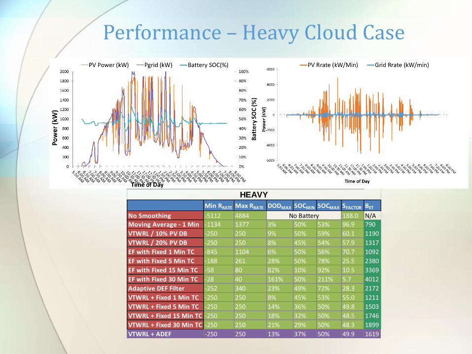
Performance – Heavy Cloud Case
Min RRATE Max RRATE DODMAX SOCMIN SOCMAX SFACTOR BET
No Smoothing -5112 4884 188.0 N/AMoving Average - 1 Min -1134 1377 3% 50% 53% 96.9 790
VTWRL / 10% PV DB -250 250 9% 50% 59% 60.1 1190
VTWRL / 20% PV DB -250 250 8% 45% 54% 57.9 1317
EF with Fixed 1 Min TC -845 1104 6% 50% 56% 70.7 1092
EF with Fixed 5 Min TC -188 261 28% 50% 78% 25.5 2380
EF with Fixed 15 Min TC -58 80 82% 10% 92% 10.5 3369
EF with Fixed 30 Min TC -28 40 161% 50% 211% 5.7 4012
Adaptive DEF Filter -252 340 23% 49% 72% 28.3 2172
VTWRL + Fixed 1 Min TC -250 250 8% 45% 53% 55.0 1211
VTWRL + Fixed 5 Min TC -250 250 14% 36% 50% 49.8 1503
VTWRL + Fixed 15 Min TC -250 250 18% 32% 50% 48.5 1746
VTWRL + Fixed 30 Min TC -250 250 21% 29% 50% 48.3 1899
VTWRL + ADEF -250 250 13% 37% 50% 49.9 1619
HEAVY
No Battery

Conclusion
• Ramp rates curtailed down to 250 kW/min in all cases.
• Up to 4x better than a 1 minute moving average
• VTWRL+ADEF allows a reduced battery size compared to existing commercial solutions.
• Smoothing is comparable or better than moving averages with
• Algorithms and equations provide a baseline for further refinement
Questions?
References:• J. Johnson, B. Schenkman, A. Ellis, J. Quiroz, and C. Lenox, "Initial Operating
Experience of the La Ola 1.2-MW Photovoltaic System," Sandia National Laboratories, Albuquerque, NM, Rep. SAND2011-8848, Oct. 2011.
• KEMA, Inc., "Research Evaluation of Wind and Solar Generation, Storage Impact, and Demand Response on the California Grid. Prepared for the California Energy Commission." KEMA CEC-500-2010-010, Jun. 2010.
• S. Atcitty, A. Baranes, A. Meintz, and B. Schenkman, “Simulation on Batteries for PV Ramp Rate Mitigation in Lanai,” 2010.
• T. Hund, S. Gonzalez, and K. Barrett, "Grid-tied pv system energy smoothing," in Photovoltaic Specialists Conference (PVSC), 2010 35th IEEE. IEEE, 2010, pp. 002 762-002 766.
• J. Bank, B. Mather, J. Keller, and M. Coddington, “High Penetration Photovoltaic Case Study Report,” National Renewable Energy Laboratory, Golden, CO, Rep. NREL/TP-5500-54742, Jan. 2013
• C. Coe., “Xtreme Power Dynamic Power Resource,” presented at the The Battery Show conference, San Jose, CA, 2010.
• A. Ellis and D. Schoenwald, “PV Output Smoothing with Energy Storage,” Sandia National Laboratories, Albuquerque, NM, Rep. SAND2012-1772, Mar. 2012.
• A. Ellis, D. Schoenwald, J. Hawkins, S. Willard, and B. Arellano, “PV Power Output Smoothing with Energy Storage,” Sandia National Laboratories, Albuquerque, NM, Rep. SAND2012-6745, Aug. 2012.
• B. Mather et al., “Southern California Edison High-Penetration Photovoltaic Project – Year 1,” National Renewable Energy Laboratory, Golden, CO, Rep. NREL/TP-5500-550875, Jun. 2011

Applicable appor,on of commodity bills eased by wearable devices
Vijaya Kumar Tukka [email protected]
Apoorv Kansal

Mo,va,on • Urbaniza,on of human civiliza,on • Shared resources and ameni,es (24/7) • Different life styles • Varying commodity prices • Pay for what you use
Source : United Na0ons, Trends in Urbaniza,on: hMp://esa.un.org/unpd/wup/Highlights/WUP2014-‐Highlights.pdf
54%
2/3
1/3
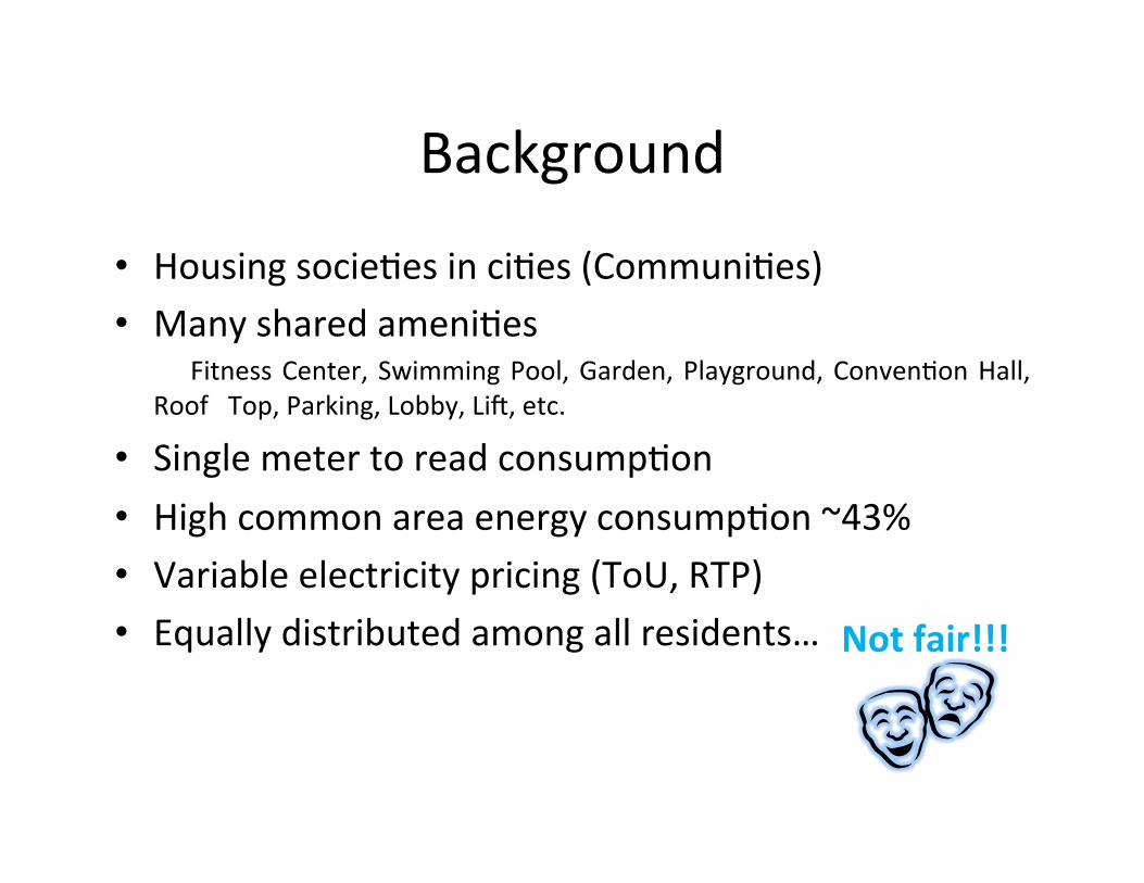
Background
• Housing socie,es in ci,es (Communi,es) • Many shared ameni,es Fitness Center, Swimming Pool, Garden, Playground, Conven,on Hall,
Roof Top, Parking, Lobby, Li], etc.
• Single meter to read consump,on • High common area energy consump,on ~43% • Variable electricity pricing (ToU, RTP) • Equally distributed among all residents…
Not fair!!!
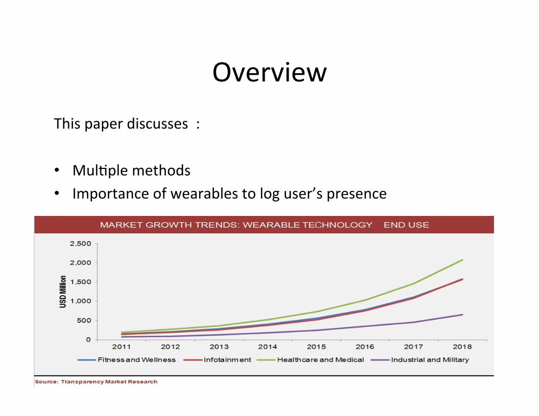
Overview This paper discusses : • Mul,ple methods • Importance of wearables to log user’s presence
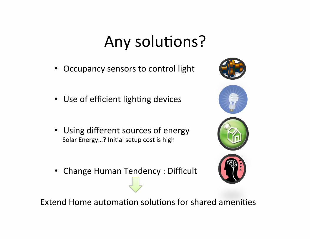
Any solu,ons?
Extend Home automa,on solu,ons for shared ameni,es
• Occupancy sensors to control light
• Use of efficient ligh,ng devices
• Using different sources of energy Solar Energy…? Ini,al setup cost is high
• Change Human Tendency : Difficult
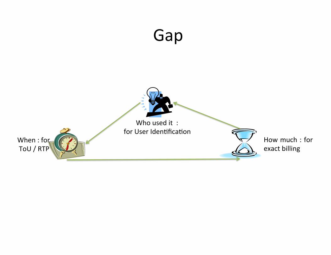
Gap
Who used it : for User Iden,fica,on
When : for ToU / RTP
How much : for exact billing
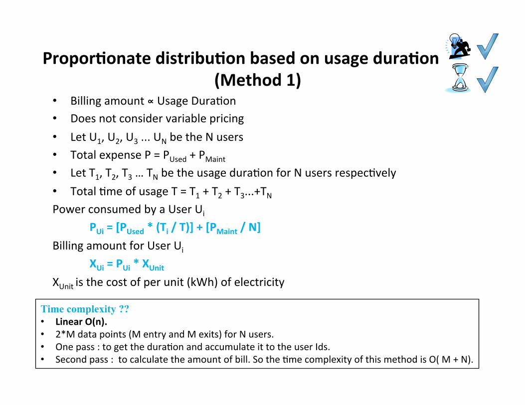
Propor0onate distribu0on based on usage dura0on (Method 1)
• Billing amount ∝ Usage Dura,on • Does not consider variable pricing • Let U1, U2, U3 ... UN be the N users • Total expense P = PUsed + PMaint
• Let T1, T2, T3 … TN be the usage dura,on for N users respec,vely • Total ,me of usage T = T1 + T2 + T3...+TN Power consumed by a User Ui PUi = [PUsed * (Ti / T)] + [PMaint / N] Billing amount for User Ui
XUi = PUi * XUnit
XUnit is the cost of per unit (kWh) of electricity
Time complexity ?? • Linear O(n). • 2*M data points (M entry and M exits) for N users. • One pass : to get the dura,on and accumulate it to the user Ids. • Second pass : to calculate the amount of bill. So the ,me complexity of this method is O( M + N).
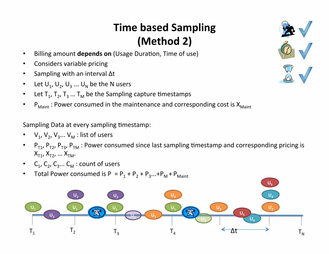
Time based Sampling (Method 2)
• Billing amount depends on (Usage Dura,on, Time of use) • Considers variable pricing • Sampling with an interval ∆t • Let U1, U2, U3 ... UN be the N users • Let T1, T2, T3 … TM be the Sampling capture ,mestamps • PMaint : Power consumed in the maintenance and corresponding cost is XMaint
Sampling Data at every sampling ,mestamp: • V1, V2, V3... VM : list of users • PT1, PT2, PT3, PTM : Power consumed since last sampling ,mestamp and corresponding pricing is
XT1, XT2, … XTM. • C1, C2, C3... CM : count of users • Total Power consumed is P = P1 + P2 + P3...+PM + PMaint
T1 T2 T3 TN ∆t
U1 U1
U2
U1
U3
U3 U3
U4
U5
U2
U1
U2
U2 U3 U1
T4
U4
U5
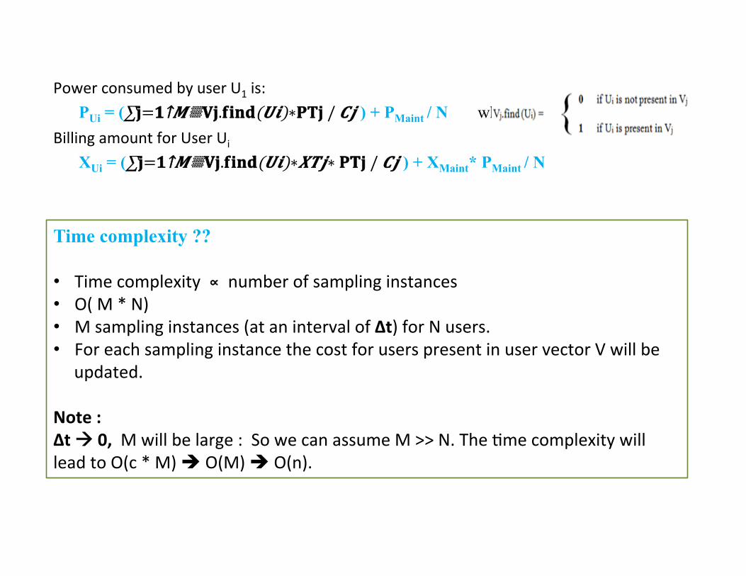
Time complexity ?? • Time complexity ∝ number of sampling instances • O( M * N) • M sampling instances (at an interval of ∆t) for N users. • For each sampling instance the cost for users present in user vector V will be
updated. Note : ∆t à 0, M will be large : So we can assume M >> N. The ,me complexity will lead to O(c * M) è O(M) è O(n).
Power consumed by user U1 is: PUi = (∑𝐣=𝟏↑𝑴▒𝐕𝐣.𝐟𝐢𝐧𝐝(𝑼𝒊)∗𝐏𝐓𝐣 / 𝑪𝒋 ) + PMaint / N where Billing amount for User Ui
XUi = (∑𝐣=𝟏↑𝑴▒𝐕𝐣.𝐟𝐢𝐧𝐝(𝑼𝒊)∗𝑿𝑻𝒋∗ 𝐏𝐓𝐣 / 𝑪𝒋 ) + XMaint* PMaint / N

Event based sampling (Method 3)
• Billing amount ∝ (Usage Dura,on, Time of use) • Considers variable pricing • Sampling at change event (Enter, Exit, Price Change) • Let U1, U2, U3 ... UN be the N users • Let {TU11, TU12}, {TU21, TU22}..., {TUN1, TUN2} be the entry / exit ,mes of N users ………(1) • TE1, TE2, …TEK : ,mestamps for electricity pricing changes ………(2) • T1, T2… TM, : Sampling ,mestamps in increasing order of ,me ………(3) • CT1, CT2 … CTM : count of users • PT1, PT2, PT3, PTM : Power consumed since last sampling ,mestamp and corresponding
pricing is XT1, XT2, … XTM.
T1 T2 T4 TN
U1
U2 U2 U3 U1 U4
U5
T5 T3 T6 T7 T8 T9
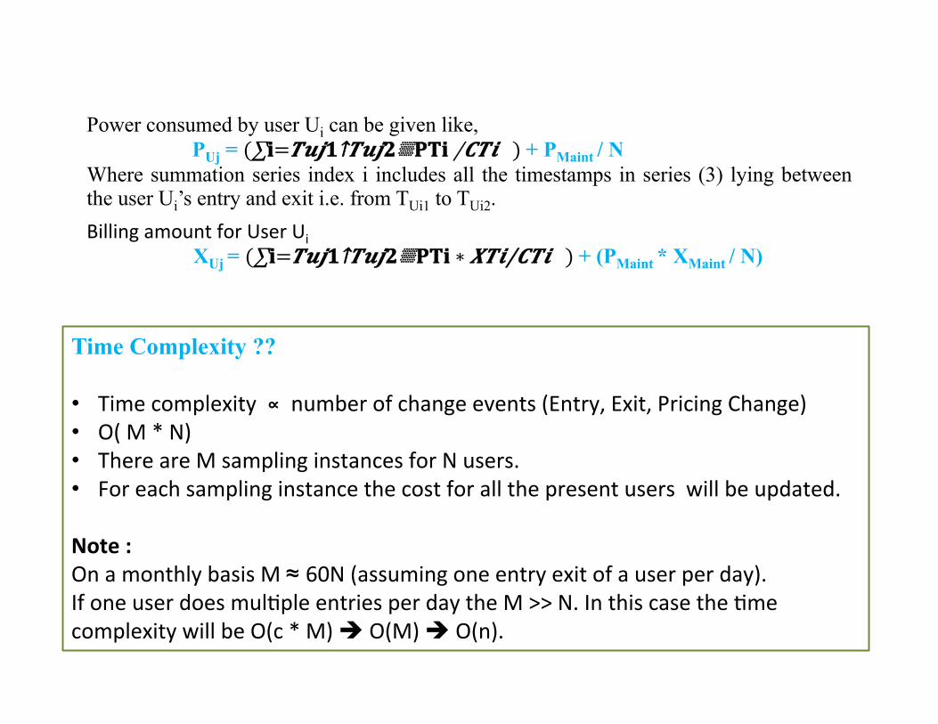
Time Complexity ??
• Time complexity ∝ number of change events (Entry, Exit, Pricing Change) • O( M * N) • There are M sampling instances for N users. • For each sampling instance the cost for all the present users will be updated. Note : On a monthly basis M ≈ 60N (assuming one entry exit of a user per day). If one user does mul,ple entries per day the M >> N. In this case the ,me complexity will be O(c * M) è O(M) è O(n).
Power consumed by user Ui can be given like, PUj = (∑𝐢=𝑻𝒖𝒋𝟏↑𝑻𝒖𝒋𝟐▒𝐏𝐓𝐢 /𝑪𝑻𝒊 ) + PMaint / N Where summation series index i includes all the timestamps in series (3) lying between the user Ui’s entry and exit i.e. from TUi1 to TUi2. Billing amount for User Ui XUj = (∑𝐢=𝑻𝒖𝒋𝟏↑𝑻𝒖𝒋𝟐▒𝐏𝐓𝐢 ∗ 𝑿𝑻𝒊/𝑪𝑻𝒊 ) + (PMaint * XMaint / N)

Analysis and Results
• Simulated data • Defined data for categories
Analysis and Results Simulated data
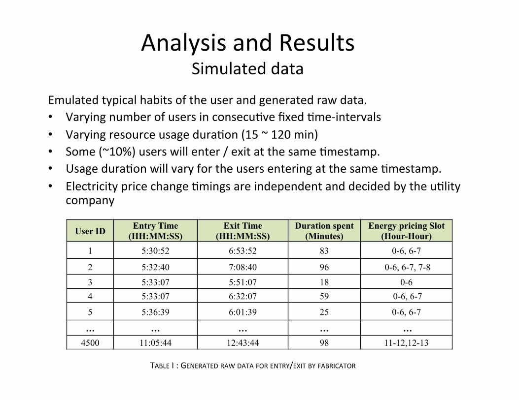
Emulated typical habits of the user and generated raw data. • Varying number of users in consecu,ve fixed ,me-‐intervals • Varying resource usage dura,on (15 ~ 120 min) • Some (~10%) users will enter / exit at the same ,mestamp. • Usage dura,on will vary for the users entering at the same ,mestamp. • Electricity price change ,mings are independent and decided by the u,lity
company
User ID Entry Time (HH:MM:SS)
Exit Time (HH:MM:SS)
Duration spent (Minutes)
Energy pricing Slot (Hour-Hour)
1 5:30:52 6:53:52 83 0-6, 6-7 2 5:32:40 7:08:40 96 0-6, 6-7, 7-8 3 5:33:07 5:51:07 18 0-6 4 5:33:07 6:32:07 59 0-6, 6-7 5 5:36:39 6:01:39 25 0-6, 6-7 … … … … …
4500 11:05:44 12:43:44 98 11-12,12-13
TABLE I : GENERATED RAW DATA FOR ENTRY/EXIT BY FABRICATOR
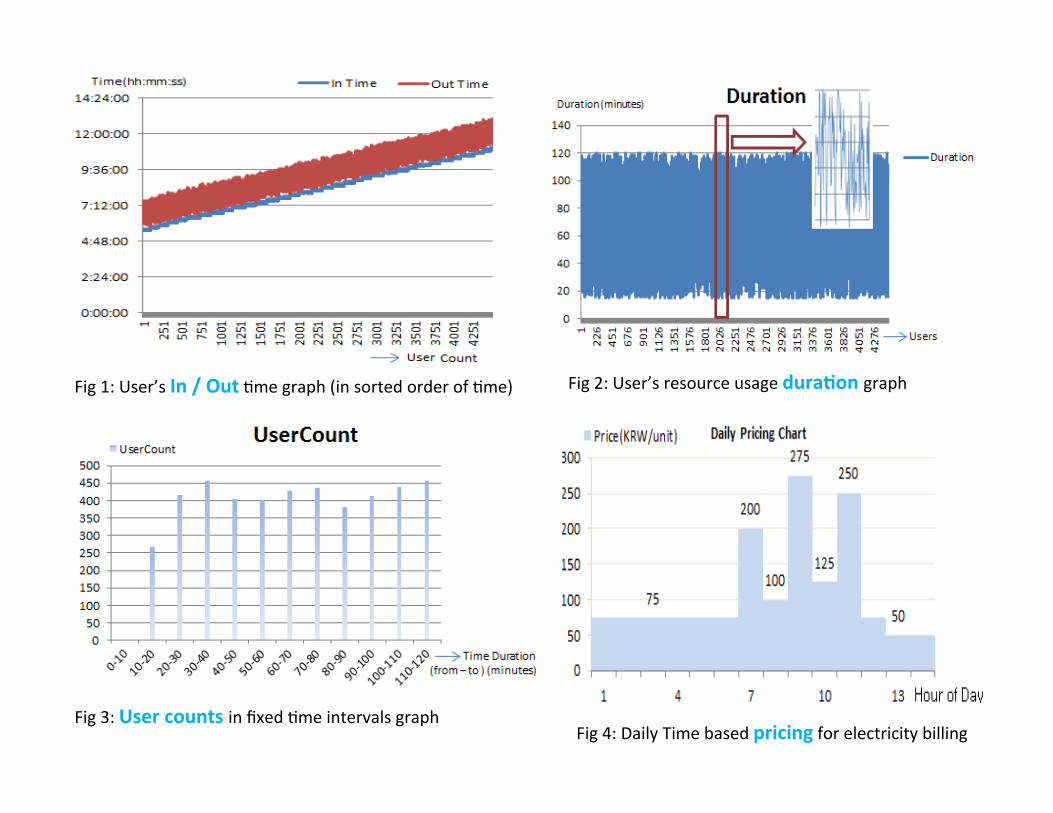
Fig 1: User’s In / Out ,me graph (in sorted order of ,me) Fig 2: User’s resource usage dura0on graph
Fig 3: User counts in fixed ,me intervals graph Fig 4: Daily Time based pricing for electricity billing
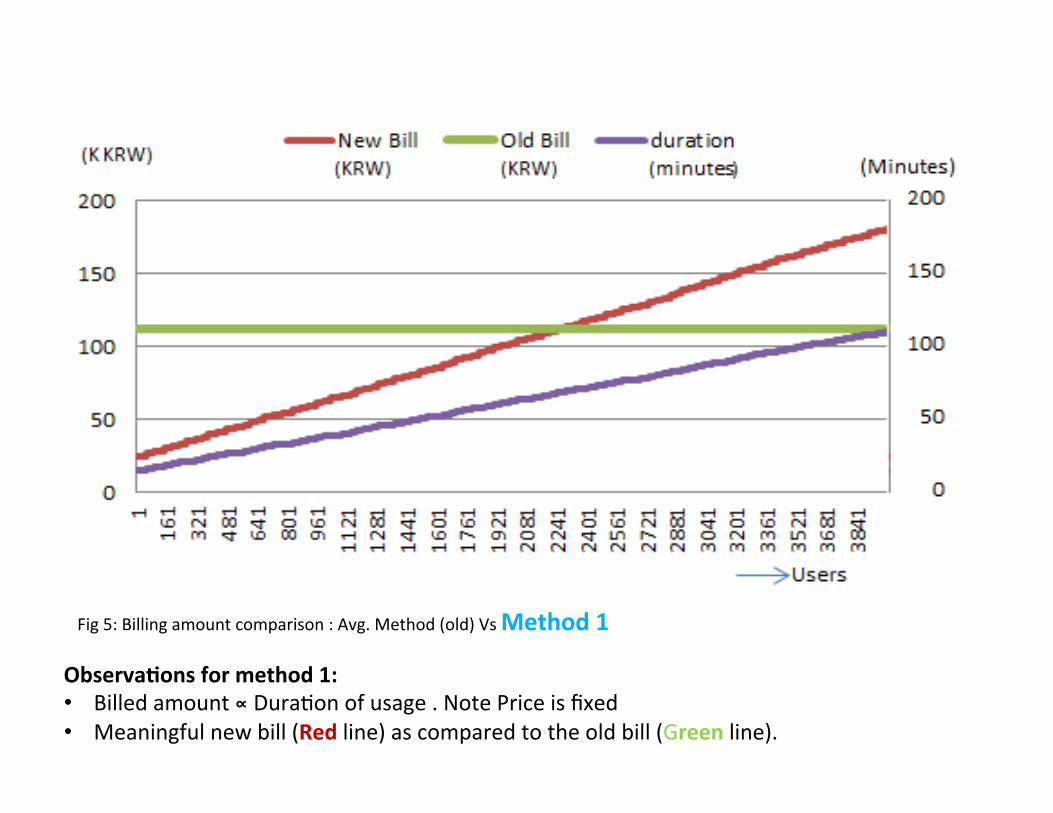
Fig 5: Billing amount comparison : Avg. Method (old) Vs Method 1
Observa0ons for method 1: • Billed amount ∝ Dura,on of usage . Note Price is fixed • Meaningful new bill (Red line) as compared to the old bill (Green line).
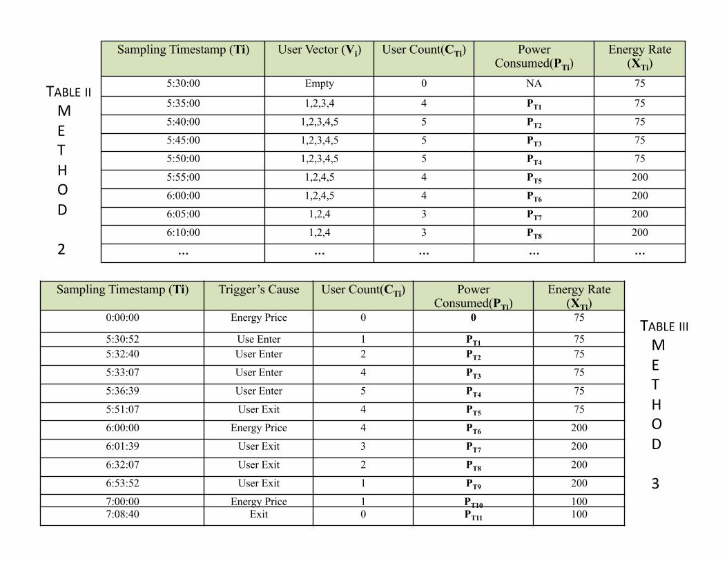
Sampling Timestamp (Ti) User Vector (Vi) User Count(CTi) Power Consumed(PTi)
Energy Rate (XTi)
5:30:00 Empty 0 NA 75
5:35:00 1,2,3,4 4 PT1 75
5:40:00 1,2,3,4,5 5 PT2 75
5:45:00 1,2,3,4,5 5 PT3 75
5:50:00 1,2,3,4,5 5 PT4 75
5:55:00 1,2,4,5 4 PT5 200
6:00:00 1,2,4,5 4 PT6 200
6:05:00 1,2,4 3 PT7 200
6:10:00 1,2,4 3 PT8 200
… … … … …
Sampling Timestamp (Ti) Trigger’s Cause User Count(CTi) Power Consumed(PTi)
Energy Rate (XTi)
0:00:00 Energy Price 0 0 75
5:30:52 Use Enter 1 PT1 75 5:32:40 User Enter 2 PT2 75
5:33:07 User Enter 4 PT3 75
5:36:39 User Enter 5 PT4 75
5:51:07 User Exit 4 PT5 75
6:00:00 Energy Price 4 PT6 200
6:01:39 User Exit 3 PT7 200
6:32:07 User Exit 2 PT8 200
6:53:52 User Exit 1 PT9 200
7:00:00 Energy Price 1 PT10 100 7:08:40 Exit 0 PT11 100
TABLE II M E T H O D 2
TABLE III M E T H O D 3
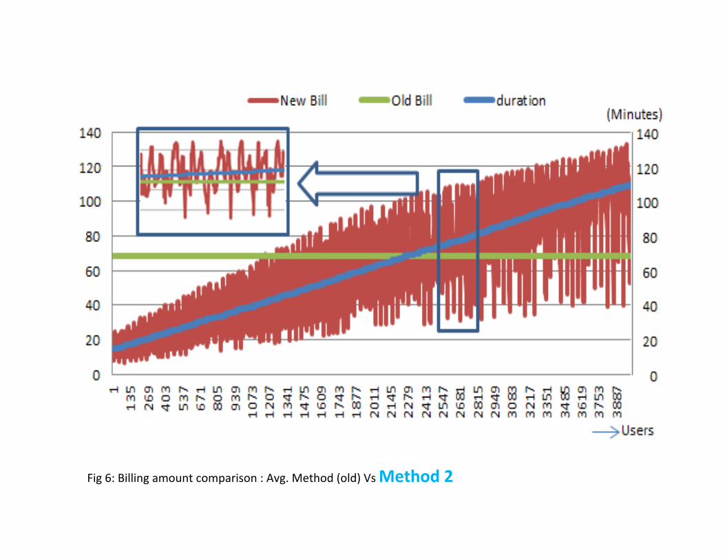
Fig 6: Billing amount comparison : Avg. Method (old) Vs Method 2
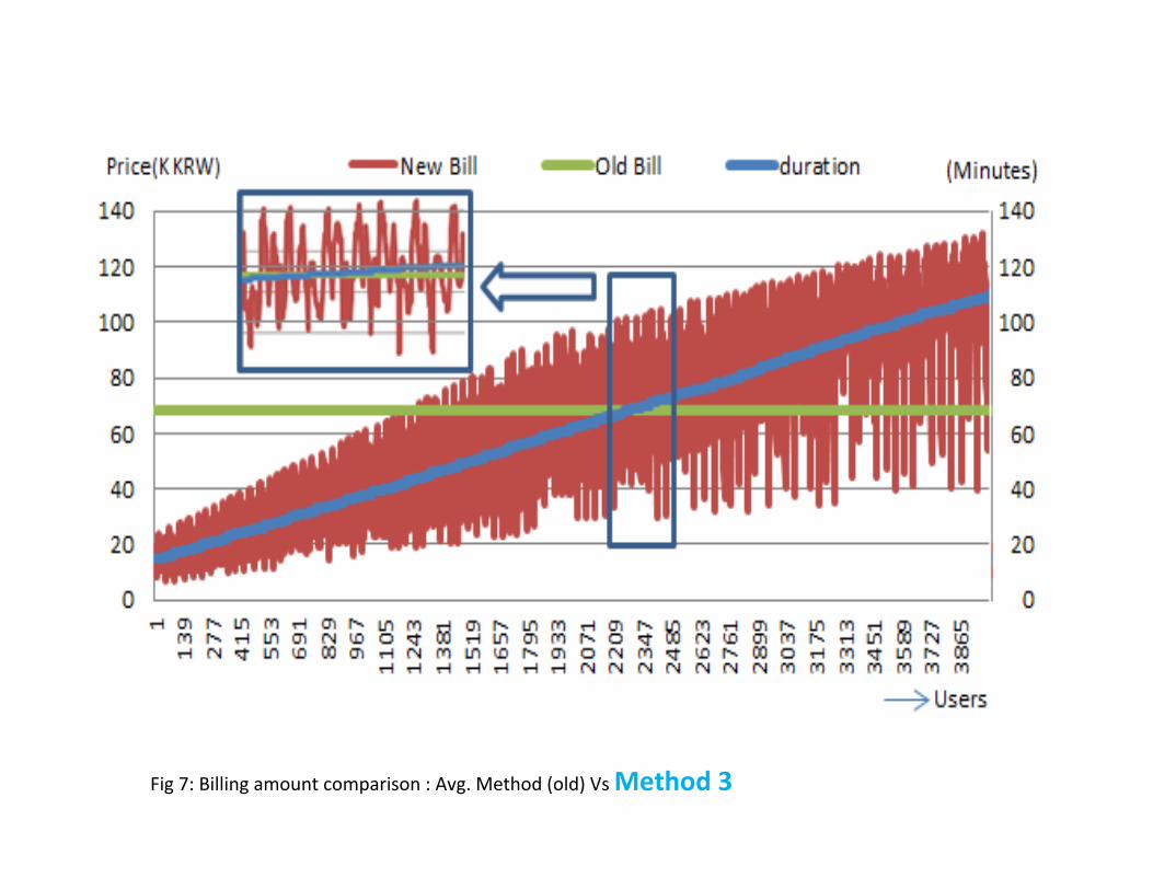
Fig 7: Billing amount comparison : Avg. Method (old) Vs Method 3
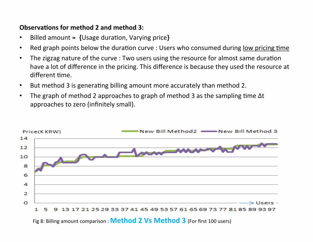
Observa0ons for method 2 and method 3: • Billed amount ∝ {Usage dura,on, Varying price} • Red graph points below the dura,on curve : Users who consumed during low pricing ,me • The zigzag nature of the curve : Two users using the resource for almost same dura,on
have a lot of difference in the pricing. This difference is because they used the resource at different ,me.
• But method 3 is genera,ng billing amount more accurately than method 2. • The graph of method 2 approaches to graph of method 3 as the sampling ,me ∆t
approaches to zero (infinitely small).
Fig 8: Billing amount comparison : Method 2 Vs Method 3 (For first 100 users)
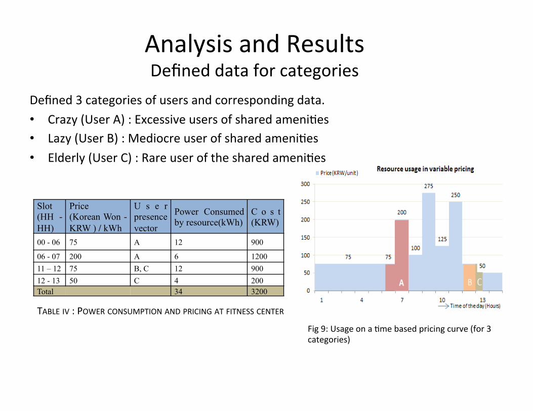
Defined 3 categories of users and corresponding data. • Crazy (User A) : Excessive users of shared ameni,es • Lazy (User B) : Mediocre user of shared ameni,es • Elderly (User C) : Rare user of the shared ameni,es
Slot (HH - HH)
Price (Korean Won - KRW ) / kWh
U s e r presence vector
Power Consumed by resource(kWh)
C o s t (KRW)
00 - 06 75 A 12 900 06 - 07 200 A 6 1200 11 – 12 75 B, C 12 900 12 - 13 50 C 4 200 Total 34 3200 TABLE IV : POWER CONSUMPTION AND PRICING AT FITNESS CENTER
Analysis and Results Defined data for categories
Fig 9: Usage on a ,me based pricing curve (for 3 categories)
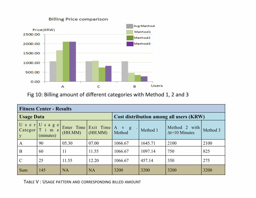
Fitness Center - Results Usage Data Cost distribution among all users (KRW) U s e r Category
U s a g e T i m e (minutes)
Enter Time (HH.MM)
Exit Time (HH.MM)
A v g . Method Method 1 Method 2 with
∆t=10 Minutes Method 3
A 90 05.30 07.00 1066.67 1645.71 2100 2100
B 60 11 11.55 1066.67 1097.14 750 825
C 25 11.55 12.20 1066.67 457.14 350 275
Sum 145 NA NA 3200 3200 3200 3200
TABLE V : USAGE PATTERN AND CORRESPONDING BILLED AMOUNT
Fig 10: Billing amount of different categories with Method 1, 2 and 3
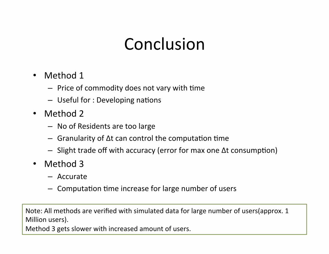
Conclusion • Method 1
– Price of commodity does not vary with ,me – Useful for : Developing na,ons
• Method 2 – No of Residents are too large – Granularity of ∆t can control the computa,on ,me – Slight trade off with accuracy (error for max one ∆t consump,on)
• Method 3 – Accurate – Computa,on ,me increase for large number of users
Note: All methods are verified with simulated data for large number of users(approx. 1 Million users). Method 3 gets slower with increased amount of users.
Future Direc,on • More analysis with real data • Large data need to consider other computa,on techniques to
reduce computa,on ,me • Make adap,ve sampling (∆t) for Method 2

Thank You