12 https://doi.org/10.1107/S205327331701614X Acta Cryst. (2018). A74, 12–24

research papers

Small-angle X-ray scattering tensor tomography:model of the three-dimensional reciprocal-spacemap, reconstruction algorithm and angularsampling requirements

Marianne Liebi,a,b,c* Marios Georgiadis,d‡ Joachim Kohlbrecher,a Mirko Holler,a

Jorg Raabe,a Ivan Usov,a Andreas Menzel,a Philipp Schneider,e Oliver Bunka and

Manuel Guizar-Sicairosa*

aPaul Scherrer Institut, 5232 Villigen PSI, Switzerland, bMAX IV Laboratory, Lund University, 221-00 Lund, Sweden,cDepartment of Physics, Chalmers University of Technology, 41296 Gothenburg, Sweden, dInstitute for Biomedical

Engineering, ETH and University Zurich, 8093 Zurich, Switzerland, and eBioengineering Science Research Group, Faculty

of Engineering and the Environment, University of Southampton, Southampton SO17 1BJ, England. *Correspondence

e-mail: marianne.liebi@chalmers.se, manuel.guizar-sicairos@psi.ch

Small-angle X-ray scattering tensor tomography, which allows reconstruction of

the local three-dimensional reciprocal-space map within a three-dimensional

sample as introduced by Liebi et al. [Nature (2015), 527, 349–352], is described in

more detail with regard to the mathematical framework and the optimization

algorithm. For the case of trabecular bone samples from vertebrae it is shown

that the model of the three-dimensional reciprocal-space map using spherical

harmonics can adequately describe the measured data. The method enables the

determination of nanostructure orientation and degree of orientation as

demonstrated previously in a single momentum transfer q range. This article

presents a reconstruction of the complete reciprocal-space map for the case of

bone over extended ranges of q. In addition, it is shown that uniform angular

sampling and advanced regularization strategies help to reduce the amount of

data required.

1. Introduction

Nanoscale features can be probed in a spatially resolved

fashion when scanning a sample through a focused X-ray

beam and recording a small-angle X-ray scattering (SAXS)

pattern at each location (Fratzl et al., 1997), a technique

referred to as scanning SAXS. The real-space resolution is

defined by the beam size and the scanning step size, which is

typically chosen in the order of several to a few tens of

micrometres, but can also be as small as some tens of nano-

metres or as large as millimetres. For each scanning point,

nanoscale features are probed in reciprocal space by the

SAXS pattern, typically measuring a spectrum of feature sizes

in the range of a few nanometres to a few hundred nano-

metres. The capability to study the distribution of nanoscale

structures over extended sample areas is of particular interest

for hierarchically structured materials for which the length

scales of interest span many orders of magnitude (Fratzl &

Weinkamer, 2007; Meyers et al., 2008; Beniash, 2011; He et al.,

2015; Van Opdenbosch et al., 2016).

A two-dimensional SAXS pattern contains statistical

information about the nanostructure within the illuminated

sample volume. If a main direction of orientation of the

nanostructure exists, it can be determined in a model-

independent way. Since a single SAXS pattern probes only a

ISSN 2053-2733

Received 14 April 2017

Accepted 8 November 2017

Edited by D. A. Keen, STFC Rutherford Appleton

Laboratory, UK

‡ Current address: Center for Biomedical

Imaging, New York University School of

Medicine, NY 10016, USA.

Keywords: small-angle X-ray scattering; tensor

tomography; spherical harmonics; bone.

two-dimensional section through the three-dimensional reci-

procal space, it provides incomplete information if the

nanostructure is anisotropic in three dimensions. The three-

dimensional orientation can be retrieved from thin sections of

a sample by measuring SAXS patterns at different rotation

angles, as illustrated in Fig. 1(a) (Liu et al., 2010; Seidel et al.,

2012; Georgiadis et al., 2015). To measure three-dimensional

samples without sectioning, scanning SAXS has to be

combined with computed tomography (CT) techniques. If the

scattering is invariant with respect to sample rotation (Feld-

kamp et al., 2009), measurements taken at different angles for

one rotation axis are enough and a standard reconstruction

algorithm, such as filtered back-projection or simultaneous

algebraic reconstruction technique (SART), can be used.

Rotational invariance applies for isotropically scattering

samples, i.e. with no preferred orientation of the nanostructure

or for unidirectional orientation of the nanostructure parallel

to the rotation axis (Schroer et al., 2006; Feldkamp et al., 2009;

Jensen et al., 2011).

Skjønsfjell et al. (2016) have shown that, with strict

assumptions on the sample, the orientation distribution can be

retrieved from measurements using a single rotation axis by

fitting a model of the X-ray scattering to the experimental

SAXS pattern. For more general anisotropically oriented

scatterers, SAXS acquisition using two rotation axes is needed

(see Fig. 1b) in order to retrieve the full three-dimensional

reciprocal-space map (Liebi et al., 2015; Schaff et al., 2015).

Schaff et al. (2015) have extended the concept of the rotation

invariance (Feldkamp et al., 2009) by the introduction of

virtual tomographic axes. After sorting the two-dimensional

SAXS patterns acquired at different rotations around two

axes into over a thousand virtual tomography axes, standard

reconstruction algorithms, here SART, are used to reconstruct

the scattering parallel to each virtual tomographic axis inde-

pendently.

Liebi et al. (2015) introduced a method based on the

modelling of the three-dimensional reciprocal-space map of

each voxel, i.e. volume element, using spherical harmonics and

minimizing the error between the measured and modelled

intensity by an optimization algorithm. The reconstruction

contains in each voxel not only a scalar value, such as the

X-ray attenuation coefficient in standard CT, but a tensor

representing the reciprocal-space map; thus the method is

referred to as SAXS tensor tomography. We present here in

more detail the mathematical framework of SAXS tensor

tomography, as introduced by Liebi et al. (2015), and the

experimental validation of the model demonstrated on

trabecular bone samples. We further investigate the angular

sampling and the number of projections required for the

reconstruction. In addition, some advanced regularization

strategies are introduced and discussed, which reduce the

amount of data and measurement time needed.

2. Model of the scattering signal using a three-dimensional reciprocal-space map

The ab initio characterization of the anisotropy of nano-

strucure in a three-dimensional volume requires measurement

of the sample from many possible orientations, not only

around one rotation axis, but in a grid of two-dimensional

orientation angles using two rotation axes. It is necessary to

define a coordinate transformation from laboratory coordi-

nates r ¼ ðx; y; zÞT, with z pointing along the direction of the

X-ray beam, to sample Cartesian coordinates r0, as illustrated

in Fig. 2. This transformation is described for the nth sample

orientation by a rotation matrix r0 ¼ Rexpn r.

The reconstruction aims to determine for each

object-coordinate voxel, r0 ¼ ðx0; y0; z0ÞT, a three-dimensional

reciprocal-space map, RRðr0; q0Þ, as a function of a reciprocal-

space vector q0 ¼ ðq0x; q0y; q0zÞT. The object-coordinate system

can also be described in spherical coordinates ðr0; �0; ’0Þ, with

�0 being the polar angle and ’0 the azimuthal angle. In order to

reach this objective, the reciprocal-space map is modelled

using spherical harmonics Yml of degree l and order m

(Jackson, 1999) as

RRðr0; q0Þ ¼Pl;m

aml ðr0; q0ÞYm

l �ðr0; q0Þ;�ðr0; q0Þ½ �

����������

2

; ð1Þ

where q0 ¼ jq0j is the magnitude of the reciprocal-space

vector, aml ðr0; q0Þ are the spherical harmonic coefficients, and

�ðr0; q0Þ and �ðr0; q0Þ are the polar and azimuthal angles,

respectively, which are arguments of the spherical harmonic

function. The square of the sum is used to avoid non-physical

negative intensities. Since spherical harmonics form a

complete basis, higher orders can be used to model the scat-

research papers

Acta Cryst. (2018). A74, 12–24 Marianne Liebi et al. � Small-angle X-ray scattering tensor tomography 13

Figure 1(a) Three-dimensional scanning SAXS setup to measure thinly slicedsamples. The sample is scanned through the focused beam in x and y atdifferent rotation angles � around y. (b) SAXS tensor tomography setupto measure three-dimensional samples. The sample is scanned throughthe focused beam in x and y at n orientations which are described by therotation matrix Rexp

n ð�; �Þ.

tering of arbitrarily complex nanostructures. For example,

spherical harmonics were used in texture analysis of pole

figures from X-ray diffraction measurements decades ago

(Roe & Krigbaum, 1964; Bunge & Roberts, 1969) using orders

up to l ¼ 36 (Van Houtte, 1983). When reconstructing a

scattering model for a large number of voxels of an extended

sample however, reducing the number of coefficients and thus

minimizing the total number of optimization parameters is of

great benefit. For cases where there is a preferential direction

of ordering for the nanostructure it is useful to orient the

zenith of the spherical harmonics to this direction indepen-

dently for each voxel in each q range. This results in a sparser

representation and reduces the number of coefficients needed

to model the reciprocal-space map. This is a particularly good

strategy in cases where the three-dimensional reciprocal-space

map is not too far from spherical or ellipsoidal symmetry; thus

only a few components are required in the decomposition of

RRðr0; q0Þ in equation (1). The local preferential orientation with

respect to the object coordinates is characterized by a unit

vector, uustr�op;’op (r0; q0), as illustrated in Fig. 2(c), which is

parameterized by the angles �opðr0; q0Þ and ’opðr

0; q0Þ. The

arguments of the spherical harmonics, �ðr0; q0Þ and �ðr0; q0Þ,

can be implicitly defined by

sin � cos �

sin � sin �

cos �

0B@

1CA ¼

cos �op cos ’op cos �op sin ’op � sin �op

� sin ’op cos ’op 0

sin �op cos ’op sin �op sin ’op cos �op

0B@

1CA

�

sin �0 cos ’0

sin �0 sin ’0

cos �0

0B@

1CA ð2Þ

where �0; ’0 are the spherical coordinates of the object-

coordinate system. Neglecting multiple-scattering effects, the

contribution of each voxel to the intensity measured at

the detector corresponds to a section through the three-

dimensional reciprocal space along the Ewald sphere of radius

2�=�. For the case of SAXS an expansion of zero order of the

Ewald sphere leads to a planar two-dimensional cut through

the reciprocal-space map, i.e. ðqx; qy; 0ÞT, in the laboratory

coordinate Cartesian system as illustrated in Fig. 2(a). The

data in the plane ðqx; qy; 0ÞT correspond to the � ¼ �=2 plane

or ðq; �=2; ’Þ in spherical coordinates. In order to calculate the

total intensity at the detector for the nth sample orientation,

the contribution from all voxels along the beam path z is

summed up,

IInðx; y; q; ’Þ ¼P

z

����Pl;m

aml ðr0; qÞ

� Yml �ðr0; qÞj�¼�=2;�ðr

0; qÞj�¼�=2

� �����2

; ð3Þ

where the measured intensity for the nth sample orientation,

IIn, is a function of the scanning position ðx; yÞ.

3. Optimization algorithm

For the reconstruction of the three-dimensional reciprocal-

space map in one specific q range, an iterative optimization

algorithm is used to minimize the error metric "q between the

modelled intensity, IIn as calculated in equation (3), with

respect to the measured data In, for all scanning positions

ðx; yÞ and sample orientations,

"q ¼ 2X

n;x;y;’

!nðx; y; q; ’Þ

� ½IInðx; y; q; ’Þ�1=2�

Inðx; y; q; ’Þ

Tnðx; yÞ

� �1=2( )2

: ð4Þ

Minimizing this error metric is a first-order approximation to a

maximum-likelihood estimation for photon-counting Poisson

noise (Thibault & Guizar-Sicairos, 2012). The measured

intensity at each point and each orientation is divided by the

transmitted intensity Tnðx; yÞ to compensate for absorption of

the sample (Schroer et al., 2006). The parameters to optimize

are the spherical harmonic coefficients, aml ðr0; q0Þ, and their

orientation through �opðr0; q0Þ and ’opðr

0; q0Þ. A binary mask,

!nðx; y; q; ’Þ, is used to denote valid data regions. It is equal to

one for all valid data points and can be set to zero for bad

detector angular sectors, ’, or where the scattering of the

sample is obstructed, for example by the sample mount.

To compute IIn we first evaluate the sum of the different

spherical harmonic terms and compute the modulus squared.

The resulting quantity is then projected along the direction of

the X-ray beam. The projection operation is calculated using

bilinear interpolation. The resulting image is convolved with a

3� 3 pyramidal kernel, which emulates the effect of up- and

subsequent down-sampling, to reduce artifacts associated with

the discrete volume grid. For the minimization of the error

metric, given in equation (4), a conjugate gradient algorithm

was used (Press et al., 2007). As the number of optimization

parameters is very large, the gradient of the error metric with

respect to the optimization parameters is calculated analyti-

cally (see Appendix A). In each iteration step the gradient is

computed according to equations (10), (11) and (14), followed

14 Marianne Liebi et al. � Small-angle X-ray scattering tensor tomography Acta Cryst. (2018). A74, 12–24

research papers

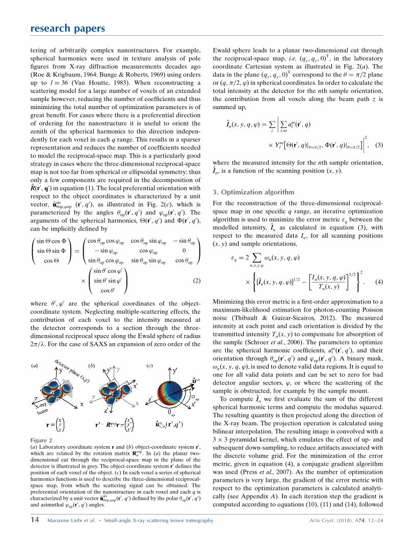
Figure 2(a) Laboratory coordinate system r and (b) object-coordinate system r0,which are related by the rotation matrix Rexp

n . In (a) the planar two-dimensional cut through the reciprocal-space map in the plane of thedetector is illustrated in grey. The object-coordinate system r0 defines theposition of each voxel of the object. (c) In each voxel a series of sphericalharmonics functions is used to describe the three-dimensional reciprocal-space map, from which the scattering signal can be obtained. Thepreferential orientation of the nanostructure in each voxel and each q ischaracterized by a unit vector uu

str�op;’opðr

0; q0Þ defined by the polar �opðr0; q0Þ

and azimuthal ’opðr0; q0Þ angles.

by a line search in a conjugate direction induced by the local

curvature of the function to be optimized [equation (4)].

In order to accelerate convergence, the optimization is

performed in four steps as illustrated in Fig. 3. First, the

isotropic component of the reciprocal-space map RRðr0; q0Þ is

optimized by using only the isotropic spherical harmonic term

with l ¼ ½0� and m ¼ ½0� and averaging the data over ’.

Secondly, only the angles are optimized and the coefficients

for l ¼ ½0 2 4�, m ¼ ½0 0 0� are kept constant at a factor s times

the a00ðr0; q0Þ obtained in the first step. For the bone

measurements shown in this paper the coefficients were set to

s ¼ 1 for a00ðr0; q0Þ, s ¼ �1=3 for a0

2ðr0; q0Þ and s ¼ 1=6 for

a04ðr0; q0Þ. These coefficients were chosen to approximate the

anisotropy which was observed in similar samples. Alter-

natively, symmetries in the three-dimensional reciprocal-space

map, which help in determining the number of spherical

harmonics functions needed, can be estimated from the shape

of the scattering object studied. Without previous knowledge

of the sample, by repeating the optimization procedure with

different constant values of the coefficients in the second step

and comparing the results, one can avoid a solution being

obtained which is just a local minimum of the error metric. It is

also possible to gain knowledge about the three-dimensional

reciprocal-space map by studying a flat sample at different

sample rotations as outlined in x4. In the third step the co-

efficients a02ðr0; q0Þ, a0

4ðr0; q0Þ and a0

6ðr0; q0Þ were optimized while

the angles and a00ðr0; q0Þ from the first step were kept constant.

Finally, in the last step all coefficients and angles were opti-

mized simultaneously.

A support constraint on the object was used in order to

optimize only the part of the object three-dimensional grid

volume which contains the sample. For this a three-

dimensional binary support mask, Mðr0Þ, is introduced,

denoting with zeros the regions without sample. This can be

obtained, for example, using a threshold after the first opti-

mization step where a first estimate of a00ðr0; q0Þ is obtained.

The mask, Mðr0Þ, is then used when computing the gradients to

set the gradients outside the object to zero, as shown in

equations (10), (11) and (14). Boundary conditions on the

values of the coefficients can be introduced either using

constrained optimization algorithms or by introducing a

smooth penalty term to the error metric. This can be used for

example to enforce symmetries if it is known that they are

present in the sample. For example, for the case of

aml ðr0; q0Þ> c

research papers

Acta Cryst. (2018). A74, 12–24 Marianne Liebi et al. � Small-angle X-ray scattering tensor tomography 15

Figure 4Two-dimensional scattering pattern in logarithmic scale obtained from athin slice of trabecular bone and a zoom-in to the low-q range. The 16segments in which the radial integration is performed are indicated bywhite lines and two circles that mark a range of q values. White trianglespoint at the pronounced first and the faint third diffraction orders ofmineralized collagen fibres.

Figure 3Flowchart of the optimization procedure. The output of the optimizationis for each object-coordinate voxel r0 the three-dimensional reciprocal-space map RRðr0; q0Þ parameterized by the preferential orientationuu

str�op;’opðr

0; q0Þ and the coefficients of the spherical harmonics aml ðr0; q0Þ.

The optimization is performed in four steps to accelerate convergence.Red dotted lines indicate starting values of the modelled intensity IIn ineach step, whereas solid red lines indicate the resulting IIn after thecorresponding optimization step. The measured intensity In is shown asblack dots; in the first step the optimization is performed using the dataaveraged over ’.

"0q ¼ "q þ �"ðpÞq þ �"

ðregÞq ð5Þ

where

"ðpÞq ¼X

r0

½aml ðr0; qÞ � c�2; if am

l ðr0; qÞ< c

0 otherwise:

�ð6Þ

Here � controls the strength of the penalty term. In the

reconstructions shown in the article, no such penalty term was

used. The regularization term, �"ðregÞq , in equation (5) will be

explained in x5.2.

4. Experimental validation of the reciprocal-spacemodel for trabecular bone

To validate the suitability of a series of spherical harmonics as

a model to describe the three-dimensional reciprocal-space

map, we used data from a 20 mm-thin section of trabecular

bone (sample A). The data were taken with a beam size of 20

� 20 mm at different rotation angles � around the y axis of the

beamline coordinate system as illustrated in Fig. 1(a). Further

experimental details can be found in Appendix B. As the

lateral resolution matches the thickness, the measurements

give an adequate representation of imaging a planar

arrangement of voxels and it has been shown that for thin

samples a single rotation axis provides sufficient information

on the three-dimensional arrangement of nanostructures

(Georgiadis et al., 2015). Image registration (Guizar-Sicairos et

al., 2008) of the transmission images, recorded simultaneously

to the SAXS data, was used to assign the scattering from

multiple orientations to individual voxels. This procedure is

described in more detail by Georgiadis et al. (2015).

Fig. 4 shows a single scattering pattern from one scan point

of the measurement. Since the nanostructure causing the

scattering has a preferential orientation, the recorded SAXS

pattern is anisotropic. Furthermore, since the nanostructure

anisotropy is three dimensional, the scattering pattern

depends on the sample orientation, � (Georgiadis et al., 2015).

The scattering from bone originates mainly from the electron-

density contrast between hydroxyapatite mineral crystal

platelets and the surrounding material with lower electron

density, such as collagen and water (Fratzl et al., 1997). The

main characteristics of the two-dimensional SAXS signal from

bone are the distinct Bragg reflections from the periodic gaps

in the collagen fibrils which are filled by hydroxyapatite

crystals (Fratzl et al., 1991). The repeat distance of these gaps

is approximately 65 nm and they produce characteristic arcs in

the scattering pattern (Wilkinson & Hukins, 1999). The first

and third harmonic of this signal are indicated by white

triangles in Fig. 4. In the direction perpendicular to these arcs

a fan-shaped scattering profile can be seen, which arises from

the shape, size and lateral arrangement of the mineral platelets

in and around the collagen fibrils (Norio et al., 1982). At high q

values, q > 0.125 nm�1, primarily the mineral platelets with an

approximate size of 3 � 25 � 50 nm can be probed. At low q

values, q < 0.1 nm�1, the scattering contains mainly informa-

tion on the lateral arrangement of the collagen fibrils and the

diameter of the fibrils, which is typically in the range of 50–

200 nm (Fratzl & Weinkamer, 2007; Gourrier et al., 2010;

Pabisch et al., 2013; Giannini et al., 2014). The organization of

bone is hierarchical: the orientation of the mineral crystals, the

collagen fibrils, the fibril bundles, the fibres and the macro-

scopic bone organization are closely related to each other

(Rinnerthaler et al., 1999; Fratzl & Weinkamer, 2007; Seidel et

al., 2012; Granke et al., 2013; Georgiadis et al., 2015, 2016).

The intensity of each scattering pattern was integrated in 16

azimuthal segments, shown by white lines in Fig. 4, for each

momentum transfer q. Increasing the number of azimuthal

segments was found to have no significant influence on the

results while increasing the amount of data and calculation

time. Black dots in Fig. 5 show the measured intensity at the

detector versus azimuthal angle ’ in one q range, 0.0379–

0.0758 nm�1, indicated by concentric circles in Fig. 4 in the 16

azimuthal segments. Symmetries, such as point symmetry, are

very common in SAXS and can be easily enforced in our

model by choosing the appropriate degrees and orders of the

spherical harmonics. For the case of trabecular bone we

assume a point symmetry around q ¼ 0 and a rotational

symmetry around one axis. Thus, using only even degree l and

zero order m is enough to model the scattering signal retrieved

from the three-dimensional reciprocal-space map. If the

mineral platelets did not point in all directions perpendicular

to the fibril axis with equal probability, the resulting

reciprocal-space map would not be a ring with cylindrical

rotational symmetry. For this case in which the rotational

symmetry is not given, higher azimuthal orders, m, of spherical

harmonics are needed to capture this feature. Fig. 5 shows for

one sample orientation, � = 20�, the intensity at the detector

versus azimuthal angle ’, for the measured and modelled data.

The azimuthal orientation of the scattering pattern can

already be described well using only degrees l ¼ ½0 2�.

However the only functional dependence allowed for these

small orders is a sine or cosine function (blue line in Fig. 5),

16 Marianne Liebi et al. � Small-angle X-ray scattering tensor tomography Acta Cryst. (2018). A74, 12–24

research papers

Figure 5SAXS measurements from a single voxel for q = (0.0379–0.0758 nm�1)for one sample rotation angle � = 20� are shown with black dots. Thecorresponding modelled data (lines) with different degrees l and zeroorder m of spherical harmonics are shown as a function of the azimuthalangle ’ in the detector plane.

which is insufficient to quantitatively model the scattering

profile, as can be seen in Fig. 5. Using l ¼ ½0 2 4� and

m ¼ ½0 0 0� (red line) the sharpness of the peak is not yet

described fully, and an artificial increase in the low-intensity

region appears. Using spherical harmonics of degree

l ¼ ½0 2 4 6� and order m ¼ ½0 0 0 0� (green line) it is possible to

reproduce reliably the measured data. Adding yet a higher

degree (yellow line) does not improve the model significantly.

Consequently, the model was applied with l ¼ ½0 2 4 6� and

m ¼ ½0 0 0 0� to reconstruct the q-resolved three-dimensional

reciprocal-space map from the data set from sample A. The

optimization was performed at 32 q values between 0.0303 and

0.984 nm�1, each with a radial width of 0.0061 nm�1. Fig. 6

shows a good agreement of the fit (points and dashed lines)

with the data (solid lines) for the full q range covered by the

two-dimensional detector. For selected q values the modelled

three-dimensional reciprocal-space map is shown. The char-

acteristic reciprocal-space footprint of the mineral platelets,

which appears as a fan-shaped profile in a two-dimensional

pattern as seen in Fig. 4, appears in the three-dimensional

reciprocal-space map as a ring perpendicular to the direction

of the fibril axis and with angular spread related to the fibrils’

degree of orientation. This ring can be observed in the whole

investigated q range in Fig. 6. The Bragg reflection, which is

associated with the collagen periodic gaps, appears in the

three-dimensional reciprocal-space map as a cap. It is visible

for the first and third harmonic of the reflection (see triangle

in Fig. 6). Using l ¼ ½0 2 4 6� and m ¼ ½0 0 0 0� is enough to

capture both features typical for the scattering from

bone. Reconstructing the full q-resolved three-dimensional

reciprocal-space map opens up the possibility of retrieving the

size and shape of the scattering object from fitting, as done in

standard small-angle scattering analysis (Bressler et al., 2015).

5. SAXS tensor tomography

In order to extend this method to volumetric samples we

combine SAXS with CT. In standard CT a scalar quantity, such

as the sample absorption, is measured for each point within

two-dimensional projections and the reconstruction is three

dimensional. In such a case it is sufficient to measure projec-

tions at different sample orientations around a single rotation

axis which is perpendicular to the X-ray beam propagation

direction. For the case of SAXS one needs a reconstruction of

the three-dimensional reciprocal-space map for each voxel, as

described by the six-dimensional function in equation (3).

Using the principles of invariant scattering along the direction

of sample rotation (Feldkamp et al., 2009), Schaff et al. (2015)

showed that for an ab initio reconstruction it is sufficient to

measure SAXS patterns from all points of the sample, while

sampling object orientations in the full 2� steradians. To

achieve this in the experiment a second rotation axis was

introduced as schematically shown in Fig. 1(b). Raster scans of

the whole sample, here also referred to as projections, are

measured at different angles � and different tilt angles of this

rotation axis, �. The object rotation matrix Rexpn in each sample

orientation n can be calculated by a rotation around y by an

angle �ðnÞ followed by a rotation around x by an angle �ðnÞ,resulting in

Rexpn ð�; �Þ ¼

cosð�Þ sinð�Þ sinð�Þ � cosð�Þ sinð�Þ0 cosð�Þ sinð�Þ

sinð�Þ � cosð�Þ sinð�Þ cosð�Þ cosð�Þ

24

35:ð7Þ

Because the sample is not perfectly aligned in the rotation

centre of both rotation axes, the translational alignment of the

measured projections has to be refined. For this purpose an

X-ray absorption tomogram is reconstructed from the

measured transmission images at � = 0�, using standard

filtered back-projection algorithms. The sample transmission

is measured simultaneously to the SAXS pattern using a

photo-diode mounted on the beamstop, which blocks the

direct unscattered beam and avoids damage to the detector.

For each object orientation, (�, �), a projection from this

absorption tomogram was calculated and used as a reference

for alignment of the measured transmission images at the

corresponding orientation. For this an efficient image regis-

tration approach based on selective up-sampling of the cross-

correlation (Guizar-Sicairos et al., 2008) was used. If the

sample has little contrast in the absorption measurement,

alternatively the scattering intensity, averaged over ’ in a

chosen q range, can be used for this step.

A human trabecular bone cylinder (sample B, Appendix B)

of about 1 mm3 was measured with a scanning step size in x

and y of 25 mm. In total n ¼ 240 projections, i.e. different

sample orientations Rexpn , were measured with an angular step

of �� = 4.5� between 0 and 180� and �� = 15� between �30

and 45�. The analysis was carried out following the procedure

as described in x3 using a q range between 0.0379 and

0.0758 nm�1.

research papers

Acta Cryst. (2018). A74, 12–24 Marianne Liebi et al. � Small-angle X-ray scattering tensor tomography 17

Figure 6Plots for measured (solid lines) and modelled (circles and dashed lines)intensity from a single voxel in two of the 16 azimuthal segments on thedetector plane. The optimization was performed in 32 q values separately.For some q values the three-dimensional reciprocal-space maps areshown mapped onto a sphere. A black triangle points towards theintensity cap characteristic of the 65 nm collagen repeat distance.

In Fig. 7 the resulting main orientation of the bone ultra-

structure is indicated by the direction of cylinders, the strength

of the isotropic component a00 by the length of cylinders, and

the degree of orientation � by the colour. The latter is

calculated by the ratio of the anisotropic component of

RRðr0; q0Þ to RRðr0; q0Þ, namely

�ðr0; q0Þ ¼R �0

R 2�

0

���P1l¼1

Plm¼�l am

l ðr0; q0ÞYm

l ð�;�Þ���2 sinð�Þ d� d�R �

0

R 2�

0

���P1l¼0

Plm¼�l am

l ðr0; q0ÞYm

l ð�;�Þ���2 sinð�Þ d� d�

¼

P1l¼1

Plm¼�l am

l ðr0; q0Þ

�� ��2P1l¼0

Plm¼�l am

l ðr0; q0Þ

�� ��2 : ð8Þ

For the reconstruction shown in Fig. 7, 830 000 SAXS patterns

were used, which were acquired in 8 h total exposure time and

an overall measurement time of 20.3 h including overhead

from motor movements. More details about the measurement

are given in Appendix B. Minimizing measurement time can

be tackled by changes in the hardware, e.g. reducing motor

scanning overhead and faster detectors (Tinti et al., 2015).

Another important aspect is to optimize spatial and angular

sampling, as discussed in the following section.

5.1. Dependence of reconstruction quality on angularsampling

In order to study the effect of the angular sampling of object

orientations on the reconstruction, the optimization proce-

dure for sample B was repeated using different subsets of the

measured angular projections n. Whereas a smaller number of

projections are used during these reconstructions, to compare

the final quality of the reconstruction Fig. 8 shows the error

with respect to all 240 projections. Therefore, the full data set

is used as a ‘gold standard’ even when only a subset of the data

is available in these test reconstructions. The whole data set is

schematically shown in Fig. 8 (in red), where each point on the

sphere represents a sample orientation and the measurements

at the six values for � are shown as six meridional rows. For

comparison, the projections from the full data set have been

removed, keeping either the original �� = 4.5� (in blue), or

�� = 15� (in black).

For the blue curve, we obtain 120 projections by taking a

subset of the data corresponding to �� = 4.5� and �� = 30�.

Furthermore, 40 projections were obtained by removing

completely the tilt of the rotation angles and keeping �� =

4.5�. In contrast, for the curve in black we label the result with

120 projections for which we increased �� to 9� and kept the

original �� = 15�, and furthermore tested 44 projections by

increasing �� to 22.5� while keeping the original �� = 15�.

That means the 40 projections (in blue) correspond to the

sampling along only one rotation axis, similar to standard

absorption-based CT, while the 44 projections (in black)

correspond to an almost isotropic angular sampling

(�� ’ ��).

The black curve with a more isotropic angular sampling

results in a lower error compared with the corresponding

points on the blue curve. The error using 120 projections

around three tilt angles �� of the rotation axis in blue is even

higher than for the 44-projection reconstruction with isotropic

angular sampling (black), even though the latter has close to

60% fewer projections. This difference can be attributed to the

angular distribution of these projections, where the 44-

projection tomogram has almost isotropic angular sampling in

� and �, and emphasizes the importance of adequate angular

sampling of the full hemisphere of sample orientations.

Following the black line, it is evident that the error metric

with respect to the full data set remains constant for an

extended range of sample rotations n, which means that the fit

to the complete data set does not change much by reducing the

number of projections, even to a fraction close to one third.

This indicates that the data set was taken with significantly

18 Marianne Liebi et al. � Small-angle X-ray scattering tensor tomography Acta Cryst. (2018). A74, 12–24

research papers

Figure 8The error according to equation (4) between the modelled intensity andall measured projections (= 240) as a function of the number ofprojections used in the optimization. The two curves show the errormetric for data sets where the projections are reduced by keepingconstant either �� (blue) or �� (black). The spherical insets show theangular sampling schematically drawn on a sphere, where each objectorientation (�, �) can be represented by a point on the hemisphere.

Figure 7Human trabecular bone (sample B). (a) Standard tomographicreconstruction based on the sample X-ray absorption. (b) Orientationof the bone ultrastructure as retrieved from SAXS tensor tomography.Colour, length and direction represent degree of orientation, isotropiccomponent a0

0 and main orientation of the collagen fibrils, respectively.

more projections than needed. One reason is that the choice of

�� = 4.5� was based on the full diameter of the sample, not

taking into account any sparsity of the sample, which could

reduce angular sampling requirements. The spatial sparsity of

the sample is actively used in the tensor tomography recon-

struction through the mask Mðr0Þ. Another form of sparsity

may arise from the fact that the bone ultrastructure exhibits

domains in the order of a few hundred micrometres. In these

reconstructions we did not use corresponding constraints.

However this domain structure is evident even from the SAXS

projections in Fig. 9. In x5.2 we show an approach to take

advantage of this knowledge through regularization.

As a validation of the reconstruction, the two-dimensional

projections from SAXS tensor reconstruction were computed

and compared with the data; in other words we compared

the measured scanning SAXS data for a projection in a

given orientation of the sample, Inðx; y; q; ’Þ, with the

corresponding projected intensity of the reconstruction,

IInðx; y; q; ’Þ. The first column in Fig. 9 shows a representation

of a scanning SAXS projection where the scattering intensity,

degree of orientation and main scattering orientation are

mapped to the image intensity, colour saturation and hue,

respectively (Bunk et al., 2009). The colour-wheel inset relates

the direction of the main scattering orientation to the parti-

cular hue. As already mentioned, it is evident that the trabe-

cular bone sample exhibits domains within which the

nanostructure orientation is spatially correlated. The

projected intensity of the reconstructions is computed using

equation (3) and shown in Fig. 9 for the case of the full data set

(n ¼ 240) and for 44 projections. By examining Fig. 9 it can be

seen that the experimental projections could be reliably

reproduced with as few as n ¼ 44 projections for this sample,

which would effectively have allowed for a reduction to one

fifth of the scanning time and the deposited dose.

5.2. Regularization strategies

In some cases there is a tendency during a reconstruction to

exacerbate high-spatial-frequency noise both in the coeffi-

cients aml ðr0; q0Þ as well as in the direction uustr

�op;’opðr0; q0Þ. To

alleviate this problem a regularization method was imple-

mented. Regularization is often used in optimization to better

research papers

Acta Cryst. (2018). A74, 12–24 Marianne Liebi et al. � Small-angle X-ray scattering tensor tomography 19

Figure 10A cross section through the three-dimensional reconstruction of the localorientation, uu

str�op;’op, is shown for (a) a reconstruction without regulariza-

tion and (b)–(f) with different values of the regularization parameter �.The three-dimensional orientation of uu

str�op;’op was encoded through both

hue and saturation, as indicated by the inset colour sphere.

Figure 9Comparison between measured two-dimensional scanning SAXS projec-tions and the equivalent projection obtained from the reconstructionusing subsets of the data corresponding to n ¼ 240 and 44 sampleorientations. The colour wheel represents the main scattering orientation,the hue the scattering intensity, and the degree of orientation the coloursaturation.

constrain ill posed or ill conditioned problems. The chosen

approach for the coefficients follows a method akin to

Grenander’s method of sieves (Grenander, 1981) by spatially

convolving the gradient with respect to the spherical harmo-

nics coefficients [equation (10)] with a three-dimensional

Hamming window. We use windows of either 3� 3� 3 or

5� 5� 5 voxels. With this method the optimization solves

first for the low and middle spatial frequencies while the high

spatial frequencies are introduced last.

For the regularization of the local preferential orientation,

uustr�op;’opðr

0; q0Þ, the gradient convolution approach is not

suitable because the direction is jointly represented by two

parameters, �opðr0; q0Þ and ’opðr

0; q0Þ. In addition, the repre-

sentation of an orientation using a vector has the inherent

ambiguity that uustr�op;’opðr

0; q0Þ and �uustr�op;’opðr

0; q0Þ would

represent the same local orientation for a reciprocal-space

map with a point symmetry. These characteristics do not pair

well with a convolution. To penalize spurious variations of the

orientation from neighbouring voxels a regularization term,

�"ðregÞq , to the error metric was introduced in equation (5). The

regularization term is based on the absolute value of the dot

product between neighbouring uustr�op;’opðr0; q0Þ, namely

"ðregÞq ¼

Pr0

h1� j uustr

�op;’opðr0; q0Þ � uustr

�op;’opðr0 þ ii; qÞ j

þ 1� j uustr�op;’opðr

0; qÞ � uustr�op;’opðr

0 þ jj; qÞ j

þ 1� j uustr�op;’opðr

0; qÞ � uustr�op;’opðr

0 þ kk; qÞ ji; ð9Þ

where ii; jj; kk are the Cartesian coordinate unit vectors, pointing

in x0; y0; z0, respectively. � is a free parameter that controls the

relative strength of the regularization.

The effect of this regularization on the orientation is shown

in Fig. 10. A trabecular bone sample (sample C) of approxi-

mately 250 mm diameter was measured with a beam of 5 �

1.4 mm and a scan step size of 5 mm with a total of 333 angular

projections, with an even distribution of projection angles ��= 7.5� and �� = 7.5� cosð�Þ according to the discussion in x5.1.

Fig. 10(a) shows an axial slice through the reconstruction of

uustr�op;’opðr

0; qÞ without regularization of the direction in which

high-spatial-frequency fluctuations of the direction between

neighbouring voxels are observed. Increasing the value of �,

Figs. 10(b)–10(f) demonstrate an increasing smoothness of the

reconstruction of uustr�op;’opðr

0; qÞ.

In order to select an appropriate regularization parameter

� the L-curve technique was applied (Hansen, 1992; Li et al.,

2003; Belge et al., 2002; Santos & Bassrei, 2007). The L-curve is

a plot of the data error, "q, versus the regularization penalty

term, "ðregÞq , where each point corresponds to different values

of the regularization strength, � (see Fig. 11a). The corner of

the L-curve corresponds to a trade-off between a smooth

solution with a high error metric "q and a solution with a small

error but more high-frequency noise (Hansen, 1992). Fig.

11(b) shows the two terms of the error metric "0q versus the

regularization parameter �. The regularization parameter

should be selected around the inflection point combined with

a visual quality inspection of the solution (Fig. 10). Here we

chose � ¼ 1� 10�3. This point is on the left side corner of the

L-curve (red arrow in Fig. 11a) because we prioritize a small

error over a smooth solution.

A three-dimensional visualization of the resulting SAXS

tensor tomography reconstruction, corresponding to Fig.

10(a), is shown in Fig. 12(b). The reconstruction using both

regularization of the coefficients, with a 5� 5� 5 Hamming

window, and of the orientation with � ¼ 1� 10�3 is shown in

Fig. 12(c). The reconstruction without regularization shows

substantial noise particularly in the orientations, and no clear

domains are visible. This variation is not supported by the

measured data, as shown in projections from different sample

orientations (�; �) in Fig. 12(a). The regularization with

� ¼ 1� 10�3 as shown in Fig. 12(c) reduced the high-

frequency noise without suppressing the different orientations

found in the sample and leads to better defined regions of a

higher degree of orientation (light green). The sample

contains different domains of orientation, each spanning some

20 Marianne Liebi et al. � Small-angle X-ray scattering tensor tomography Acta Cryst. (2018). A74, 12–24

research papers

Figure 11(a) L-curve used to find an appropriate regularization parameter �. (b)shows the dependence of the penalty term "ðregÞ

q (left black axis) and of theof error metric "q (right blue axis) on the regularization parameter �.These two values are combined in the L-curve. The red arrow and reddashed line indicate the regularization parameter selected for thistrabecular bone sample as explained in the text.

tens of micrometres, similar to the sample shown in Figs. 7 and

9. The higher resolution obtained here with a smaller beam

size of 5 � 1.4 mm enables us to resolve the transition region

between the domains.

6. Conclusion

SAXS tensor tomography aims at reconstructing the local

three-dimensional reciprocal-space map for each volume

element within a three-dimensional sample. This can be

achieved through gradient-based optimization. An adequate

numerical representation of the three-dimensional reciprocal-

space map, for which only a few quantities or coefficients have

to be recovered for each voxel, can be critical towards

developing an approach that is efficient both in computational

and measurement time. Liebi et al. (2015) introduced this

reconstruction approach using spherical harmonics as a base

to represent the reciprocal-space map and demonstrated it

with a millimetre-sized sample of trabecular bone. The three-

dimensional reciprocal-space map comprises information on

the main orientation of the nanostructure for different q

ranges and also its degree of orientation. The reciprocal-space

map could further be used as input for fitting the underlying

nanostructure, similarly to what has been done on two-

dimensional SAXS data, for example to retrieve size para-

meters of the mineralized platelets in bone (Fratzl et al., 2005;

Turunen et al., 2016).

In this article we present a detailed description of the

algorithm as well as a validation study to confirm the suit-

ability of spherical harmonic coefficients to represent the

three-dimensional reciprocal-space map of trabecular bone

where the features of the mineralized collagen fibrils can be

recovered. In order to reduce the number of coefficients that

need to be optimized we provide for each voxel a para-

meterization of the spherical harmonic zenith direction, which

provides directly the orientation of the main symmetry axis of

the nanostructure in three dimensions and subsequently

allows us to impose reciprocal-space symmetry constraints.

Regularization strategies for both the coefficients and the

orientation are introduced and described in detail. An

important consideration is the distribution of projection

angles for the measurements. By selectively removing angles

the effect on the reconstruction is shown, which confirms that

a uniform distribution of sample orientations is of significant

benefit for the reconstruction quality.

SAXS tensor tomography provides a technique that can

probe three-dimensional nanostructure information in rela-

tively large volumes, offering the unique chance to correlate

spatial nanoscale features over several millimetres, i.e. sepa-

rated over five or six orders of magnitude. The technique is

applicable to a wide range of specimens in biology and

materials science and also scalable. While the original

demonstration was with 20 mm voxel size, by using micro-

focusing optics and improved scanning hardware this article

demonstrated the technique to a spatial resolution of 5 mm. By

suitable changes in optics and hardware the resolution can be

adjusted to the application of interest.

APPENDIX AAnalytical expressions for the gradients

The gradient of the error metric "q, as defined in equation (4),

with respect to the spherical harmonic coefficients is given by

@"q

@aml ðr0; qÞ¼ 4Mðr0Þ

Xn;’

!nðx; y; q; ’Þ

�

½IInðx; y; q; ’Þ�1=2�

Inðx;y;q;’ÞTnðx;yÞ

h i1=2

½IInðx; y; q; ’Þ�1=2

8><>:

9>=>;

� Yml �ðr0; qÞ j�¼�=2;�ðr

0; qÞ j�¼�=2

� ��Xl0;m0

am0

l0 ðr0; qÞYm0

l0 �ðr0; qÞ j�¼�=2;�ðr0; qÞ j�¼�=2

� �ð10Þ

where the notation �ðr0; qÞ j�¼�=2 indicates that the function is

evaluated at the detector plane, � ¼ �=2, in the laboratory

coordinates r, and with q0 ¼ q. Notice that the first term in

brackets in equation (10) is only a function of ðx; yÞ in the

laboratory coordinates r and that it is constant along the z

direction, which is effectively a back-projection. This is then

computed via back-projection along the beam-propagation

direction using bilinear interpolation.

research papers

Acta Cryst. (2018). A74, 12–24 Marianne Liebi et al. � Small-angle X-ray scattering tensor tomography 21

Figure 12Orientation of the bone ultrastructure from a human trabecular bone(sample C). Four two-dimensional SAXS projections at different sampleorientations are shown in (a), where the colour wheel represents the mainscattering orientation, the hue the scattering intensity and the degree oforientation the colour saturation. The orientation of the boneultrastructure retrieved from SAXS tensor tomography is shown in (b)and (c), where the colour represents the degree of orientation and thelength of the isotropic component a0

0. (b) Reconstruction withoutregularization applied and (c) with regularization of the sphericalharmonics coefficients am

l ðr0; q0Þ and on the direction uu

str�op;’op as described

in the text.

The gradient with respect to �opðr0; qÞ is given by

@"q

@�opðr0; qÞ¼ 4Mðr0Þ

Xn;’

!nðx; y; q; ’Þ

�

½IInðx; y; q; ’Þ�1=2�

Inðx;y;q;’ÞTnðx;yÞ

h i1=2

½IInðx; y; q; ’Þ�1=2

8><>:

9>=>;

�

"@Ym

l ð�;�Þ

@�

@�ðr0; qÞ j�¼�=2

@�opðr0; qÞ

þ@Ym

l ð�;�Þ

@�

@�ðr0; qÞ j�¼�=2

@�opðr0; qÞ

#

�Xl0;m0

am0

l0 ðr0; qÞYm0

l0 ½�ðr0; qÞ j�¼�=2;�ðr

0; qÞ j�¼�=2�:

ð11Þ

The derivatives of the spherical harmonic functions are given

by (Wolfram Research Inc., 2017a,b)

@Yml ð�;�Þ

@�¼ mYm

l ð�;�Þ cot �þ ½ðl �mÞðl þmþ 1Þ�1=2

� expð�i�ÞYmþ1l ð�;�Þ; ð12aÞ

@Yml ð�;�Þ

@�¼ imYm

l ð�;�Þ: ð12bÞ

Using equation (2)

@�ðr0; qÞ j�¼�=2

@�opðr0; qÞ

¼1

r0 sin �ðr0; qÞ j�¼�=2

fz0 sin �opðr0; qÞ

� ½x0 cos ’opðr0; qÞ þ y0 sin ’opðr

0; q�

� cos �opðr0; qÞg j�¼�=2; ð13aÞ

@�ðr0; qÞ j�¼�=2

@�opðr0; qÞ

¼ cos2 �ðr0; qÞ j�¼�=2 f�x02

cos ’opðr0; qÞ

� 2y02

cos �opðr0; qÞ sin �opðr

0; qÞ sin ’opðr0; qÞ

� x0y0 sin ’opðr0; qÞ½sin2 �opðr

0; qÞ � cos2 �opðr0; qÞ� þ y0z0g

=½x0 cos �opðr0; qÞ cos ’opðr

0; qÞ þ y0 cos �opðr0; qÞ sin ’opðr

0; qÞ

� z0 sin �opðr0; qÞ�2j�¼�=2: ð13bÞ

Similarly, the gradient with respect to ’opðr0; qÞ is given by

@"q

@’opðr0; qÞ¼ 4Mðr0Þ

Xn;’

!nðx; y; q; ’Þ

�

(½IInðx; y; q; ’Þ�1=2

�Inðx;y;q;’Þ

Tnðx;yÞ

h i1=2

½IInðx; y; q; ’Þ�1=2

)

�

"@Ym

l ð�;�Þ

@�

@�ðr0; qÞ j�¼�=2

@’opðr0; qÞ

þ@Ym

l ð�;�Þ

@�

@�ðr0; qÞ j�¼�=2

@’opðr0; qÞ

#

�Xl0;m0

am0

l0 ðr0; qÞYm0

l0 ½�ðr0; qÞ j�¼�=2;�ðr

0; qÞ j�¼�=2�

ð14Þ

with

@�ðr0; qÞ j�¼�=2

@’opðr0; qÞ

¼sin �opðr

0; qÞ

r0 sin �ðr0; qÞ j�¼�=2Þ

� ½x0 sin ’opðr0; qÞ � y0 cos ’opðr

0; qÞ� j�¼�=2;

ð15aÞ

@�ðr0; qÞ j�¼�=2

@’opðr0; qÞ

¼ cos2 �ðr0; qÞ j�¼�=2

� ½x0 sin �opðr0; qÞ � y0 cos �opðr

0; q�

� ½�x0 cos �opðr0; qÞ sin ’opðr

0; qÞ þ y0 cos �opðr0; qÞ cos ’opðr

0; q�

=½x0 cos �opðr0; qÞ cos ’opðr

0; qÞ þ y0 cos �opðr0; qÞ sin ’opðr

0; qÞ

� z0 sin �opðr0; qÞ�2 j�¼�=2 : ð15bÞ

Using this gradient and the previous search direction a

conjugate gradient direction is defined, and along this direc-

tion a line search is carried out to look for the minimum value

of the error metric (Press et al., 2007).

If the smooth penalty term "ðpÞq is introduced in the error

metric as described in equations (5) and (6), the gradient of

the error metric with respect to the spherical harmonic co-

efficients [equation (10)] is

@"0q@am

l ðr0; qÞ¼

@"q

@aml ðr0; qÞþ �

@"ðpÞq

@aml ðr0; qÞ

ð16Þ

with

@"ðpÞq

@aml ðr0; qÞ¼X

r0

(2½am

l ðr0; qÞ � c�; if am

l ðr0; qÞ< c

0 otherwise:ð17Þ

If regularization of the local preferential orientation

uustr�op;’opðr

0; qÞ is used, the gradient with respect to �opðr0; qÞ is

@"0q@�opðr

0; qÞ¼

@"q

@�opðr0; qÞþ �

@"ðregÞq

@�opðr0; qÞ

ð18Þ

with

22 Marianne Liebi et al. � Small-angle X-ray scattering tensor tomography Acta Cryst. (2018). A74, 12–24

research papers

@"ðregÞq

@�opðr0; qÞ¼X

r0

"�@ j uu

str�op;’opðr

0; qÞ � uustr�op;’opðr

0 þ ii; qÞ j

@�opðr0; qÞ

�@ j uu

str�op;’opðr

0; qÞ � uustr�op;’opðr

0 þ jj; qÞ j

@�opðr0; qÞ

�@ j uu

str�op;’opðr

0; qÞ � uustr�op;’opðr

0 þ kk; qÞ j

@�opðr0; qÞ

#; ð19Þ

with

@ j uustr�op;’opðr

0; qÞ � uustr�op;’opðr

0 þ ii; qÞ j

@�opðr0; qÞ

¼

uustr�op;’opðr

0; qÞ � uustr�op;’opðr

0 þ ii; qÞ

j uustr�op;’opðr

0; qÞ � uustr�op;’opðr

0 þ ii; qÞ j

��

cos½’opðr0; qÞ þ ’opðr

0 þ ii; qÞ� cos �opðr0; qÞ

� sin �opðr0þ ii; qÞ þ cos½’opðr

0; qÞ þ ’opðr0� ii; qÞ�

� sin �opðr0� ii; qÞ cos’opðr

0; qÞ þ ½� sin �opðr0; qÞ

� cos �opðr0þ ii; qÞ � cos �opðr

0� ii; qÞ sin �opðr

0; q�:

ð20Þ

Similarly, expressions for the terms with finite differences in

the y and z directions can be obtained to complete equation

(19). Equivalent expressions can be found for the gradient

with respect to ’opðr0; qÞ.

APPENDIX BExperimental details

B1. Sample preparation

Trabeculas from a 12th thoracic (T12) human vertebra from

a 50-year-old woman (sample A) and a 73-year-old man

(samples B and C) were extracted and soft tissue was removed

before embedding into polymethyl methacrylate (PMMA).

The vertebrae were obtained from the Department of

Anatomy, Histology and Embryology at the Innsbruck

Medical University, Innsbruck, Austria, with the written

consent of the donors according to Austrian law. All of the

following procedures were performed in accordance with

Swiss law, the Guideline on Bio-Banking of the Swiss

Academy of Medical Science (2006) and the Swiss ordinance

814.912 (2012) on the contained use of organisms. To obtain

sample A, a 20 mm-thick section was cut using a microtome

(HM 355S; Thermo Fisher Scientific Inc., USA) and mounted

on 12 mm-thick Kapton adhesive tape (T2000023; Benetec,

Wettswil, Switzerland). A cylinder of about 1 mm and 250 mm

diameter was milled out of the PMMA block for samples B

and C, respectively.

B2. Experiments

Measurements were performed at the coherent small-angle

X-ray scattering (cSAXS) beamline (X12SA) of the Swiss

Light Source, Paul Scherrer Institut, Switzerland. The X-ray

beam was monochromated by a fixed-exit double-crystal

Si(111) monochromator to 12.4 keV for samples A and B, and

to 11.2 keV X-ray energy for sample C. Two different types of

focusing were used. For samples A and B the beam was

focused horizontally by bending the second monochromator

crystal and vertically by bending a Rh-coated mirror resulting

in a beam size of about 20 � 20 mm and 25 � 25 mm,

respectively. For sample C the beam was focused with a

Fresnel zone plate to a beam size of 5� 1.4 mm (Lebugle et al.,

2017). To minimize air scattering and X-ray absorption a 7 m

(samples A and B) or a 2 m long (sample C) flight tube was

placed between the sample and detector. X-ray scattering was

measured with a Pilatus 2M detector (Kraft et al., 2009) and

the transmitted-beam intensity with a photo-diode mounted

on a beamstop placed inside the flight tube.

Sample A, a thin section of trabecular bone, was measured

in the three-dimensional scanning SAXS setup as described by

Georgiadis et al. (2015) and schematically shown in Fig. 1(a).

The sample was mounted on a goniometer placed on a rota-

tion stage on top of a two-axis translation stage. The sample

was continuously moved in the x direction while SAXS

patterns were measured with 50 ms exposure time. The scan

was repeated at 30 different sample orientations around the y

axis in steps of 10�, omitting the angles where the section was

close to parallel to the X-ray beam, i.e. 80–100� and 260–280�.

The scan step in x was chosen to be 20 cosð�Þ mm to have a

consistent number of scanning points across the specimen. The

scan step in y was 20 mm. To identify the scattering that

originates from a specific voxel under all sample rotation

angles, image registration (Guizar-Sicairos et al., 2008) on the

transmission images was used, as described in detail by

Georgiadis et al. (2015).

Samples B and C were measured with the three-

dimensional tensor tomography setup as described by Liebi et

al. (2015) and schematically shown in Fig. 1(b). The sample

was mounted on a goniometer on two perpendicular rotation

stages which were placed on a two-axis scanning stage.

Sample B was measured at n ¼ 240 projections, each with

55� 65 scanning steps with a step size of 25 mm. The sample

was continuously moved in the x direction while SAXS

patterns were measured with an exposure time of 30 ms, which

was limited by the detector read-out. The angular spacing was

15� between�30� and 45� in � and 4.5� between 0� and 180� in

�. The total exposure time was 8.3 h. Each voxel was exposed

for a total of 7.2 s. Because of overhead from motor move-

ment, the total measurement time was 20.3 h.

Sample C was measured at n ¼ 333 projections, each with

85� 65 scanning steps with a step size of 5 mm and an expo-

sure time of 50 ms. As the beam in the vertical (y) was smaller

than the step size, the sample was continuously moved in the y

direction during measurement in order to probe the whole

sample volume. Based on our findings with regard to the

advantage of an even distribution of projection angles �� =

7.5� and �� = 7.5� cosð�Þ have been used. The total exposure

time was 11.8 h and the total measurement time 21.3 h. The

overhead of motor movements was reduced compared with

the measurement of sample B, mainly by introducing a snake-

like scan pattern where subsequent lines are scanned in

research papers

Acta Cryst. (2018). A74, 12–24 Marianne Liebi et al. � Small-angle X-ray scattering tensor tomography 23

opposite directions, which reduces the time the motor needs to

reach the line scan starting position. Additional projections

were measured at � ¼ 0, achieving �� = 3� to have enough

projections for the standard filtered back-projection recon-

struction used for image registration as described in x5.

B3. Availability of the software

A current version of the data analysis software is available

upon request from the corresponding authors.

Acknowledgements

We thank A. Diaz, F. Schaff and M. Bech for discussions and

A. E. Louw-Gaume for proofreading. The vertebral specimen

was provided by W. Schmolz, Department for Trauma Surgery,

Innsbruck Medical University, Innsbruck, Austria. We also

thank the anonymous reviewers whose input helped improve

this paper significantly. MG was supported by the ETH

Research Grant No. ETH-39 11-1. ML acknowledges financial

support from the Area of Advance Materials Science at

Chalmers University of Technology. We acknowledge support

from the Data Analysis Service (142-004) project of the

swissuniversities SUC P-2 program.

References

Belge, M., Kilmer, M. E. & Miller, E. L. (2002). Inverse Probl. 18,1161–1183.

Beniash, E. (2011). WIREs Nanomed. Nanobiotechnol. 3, 47–69.http://dx.doi.org/10.1002/wnan.105.

Breßler, I., Kohlbrecher, J. & Thunemann, A. F. (2015). J. Appl. Cryst.48, 1587–1598.

Bunge, H.-J. & Roberts, W. T. (1969). J. Appl. Cryst. 2, 116–128.Bunk, O., Bech, M., Jensen, T. H., Feidenhans’l, R., Binderup, T.,

Menzel, A. & Pfeiffer, F. (2009). New J. Phys. 11, 123016.Feldkamp, J. M., Kuhlmann, M., Roth, S. V., Timmann, A., Gehrke,

R., Shakhverdova, I., Paufler, P., Filatov, S. K., Bubnova, R. S. &Schroer, C. G. (2009). Phys. Status Solidi A, 206, 1723–1726.

Fratzl, P., Fratzl-Zelman, N., Klaushofer, K., Vogl, G. & Koller, K.(1991). Calcif. Tissue Int. 48, 407–413.

Fratzl, P., Gupta, H. S., Paris, O., Valenta, A., Roschger, P. &Klaushofer, K. (2005). Diffracting Stacks of Cards – Some Thoughtsabout Small-Angle Scattering from Bone, pp. 33–39. Berlin,Heidelberg: Springer.

Fratzl, P., Jakob, H. F., Rinnerthaler, S., Roschger, P. & Klaushofer, K.(1997). J. Appl. Cryst. 30, 765–769.

Fratzl, P. & Weinkamer, R. (2007). Prog. Mater. Sci. 52, 1263–1334.Georgiadis, M., Guizar-Sicairos, M., Gschwend, O., Hangartner, P.,

Bunk, O., Muller, R. & Schneider, P. (2016). PLoS One, 11,e0159838.

Georgiadis, M., Guizar-Sicairos, M., Zwahlen, A., Trussel, A. J., Bunk,O., Muller, R. & Schneider, P. (2015). Bone, 71, 42–52.

Giannini, C., Siliqi, D., Ladisa, M., Altamura, D., Diaz, A., Beraudi,A., Sibillano, T., De Caro, L., Stea, S., Baruffaldi, F. & Bunk, O.(2014). J. Appl. Cryst. 47, 110–117.

Gourrier, A., Li, C., Siegel, S., Paris, O., Roschger, P., Klaushofer, K.& Fratzl, P. (2010). J. Appl. Cryst. 43, 1385–1392.

Granke, M., Gourrier, A., Rupin, F., Raum, K., Peyrin, F.,Burghammer, M., Saıed, A. & Laugier, P. (2013). PLoS One, 8,e58043.

Grenander, U. (1981). Abstract Inference. New York: Wiley.Guizar-Sicairos, M., Thurman, S. T. & Fienup, J. R. (2008). Opt. Lett.

33, 156–158.

Hansen, P. C. (1992). SIAM Rev. 34, 561–580.He, W.-X., Rajasekharan, A. K., Tehrani-Bagha, A. R. & Andersson,

M. (2015). Adv. Mater. 27, 2260–2264.Jackson, J. D. (1999). Classical Electrodynamics, 3rd ed. New York:

Wiley.Jensen, T. H., Bech, M., Bunk, O., Thomsen, M., Menzel, A., Bouchet,

A., Le Duc, G., Feidenhans’l, R. & Pfeiffer, F. (2011). Phys. Med.Biol. 56, 1717–1726.

Kraft, P., Bergamaschi, A., Broennimann, Ch., Dinapoli, R.,Eikenberry, E. F., Henrich, B., Johnson, I., Mozzanica, A.,Schleputz, C. M., Willmott, P. R. & Schmitt, B. (2009). J.Synchrotron Rad. 16, 368–375.

Lebugle, M., Liebi, M., Wakonig, K., Guzenko, V. A., Holler, M.,Menzel, A., Guizar-Sicairos, M., Diaz, A. & David, C. (2017). Opt.Express, 25, 21145–21158.

Li, A., Miller, E. L., Kilmer, M. E., Brukilacchio, T. J., Chaves, T.,Stott, J., Zhang, Q., Wu, T., Chorlton, M., Moore, R. H., Kopans, D.B. & Boas, D. A. (2003). Appl. Opt. 42, 5181–5190.

Liebi, M., Georgiadis, M., Menzel, A., Schneider, P., Kohlbrecher, J.,Bunk, O. & Guizar-Sicairos, M. (2015). Nature, 527, 349–352.

Liu, Y. F., Manjubala, I., Roschger, P., Schell, H., Duda, G. N. & Fratzl,P. (2010). XIV International Conference on Small-Angle Scattering(Sas09), Journal of Physics Conference Series, Vol. 247, p. 9. Bristol:Institute of Physics Publishing. http://dx.doi.org/10.1088/1742-6596/247/1/012031

Meyers, M. A., Chen, P.-Y., Lin, A. Y.-M. & Seki, Y. (2008). Prog.Mater. Sci. 53, 1–206.

Norio, M., Morio, A. & Yoshio, T. (1982). Jpn. J. Appl. Phys. 21,186.

Pabisch, S., Wagermaier, W., Zander, T., Li, C. H. & Fratzl, P. (2013).Imaging the Nanostructure of Bone and Dentin Through Small- andWide-angle X-ray Scattering. Methods in Enzymology, Vol. 532, pp.391–413. San Diego: Elsevier Academic Press Inc.

Press, W. H., Teukolsky, S. A., Vetterling, W. T. & Flannery, B. P.(2007). Numerical Recipes, 3rd ed., The Art of Scientific Computing.Cambridge University Press.

Rinnerthaler, S., Roschger, P., Jakob, H. F., Nader, A., Klaushofer, K.& Fratzl, P. (1999). Calcif. Tissue Int. 64, 422–429.

Roe, R. & Krigbaum, W. R. (1964). J. Chem. Phys. 40, 2608–2615.Santos, E. T. F. & Bassrei, A. (2007). Comput. Geosci. 33, 618–

629.Schaff, F., Bech, M., Zaslansky, P., Jud, C., Liebi, M., Guizar-Sicairos,

M. & Pfeiffer, F. (2015). Nature, 527, 353–356.Schroer, C. G., Kuhlmann, M., Roth, S. V., Gehrke, R., Stribeck, N.,

Almendarez-Camarillo, A. & Lengeler, B. (2006). Appl. Phys. Lett.88, 164102.

Seidel, R., Gourrier, A., Kerschnitzki, M., Burghammer, M., Fratzl, P.,Gupta, H. S. & Wagermaier, W. (2012). Bioinspired BiomimeticNanobiomater. 1, 123–131. http://dx.doi.org/10.1680/bbn.11.00014.

Skjønsfjell, E. T., Kringeland, T., Granlund, H., Høydalsvik, K., Diaz,A. & Breiby, D. W. (2016). J. Appl. Cryst. 49, 902–908.

Thibault, P. & Guizar-Sicairos, M. (2012). New J. Phys. 14, 063004.Tinti, G., Bergamaschi, A., Cartier, S., Dinapoli, R., Greiffenberg, D.,

Johnson, I., Jungmann-Smith, J. H., Mezza, D., Mozzanica, A.,Schmitt, B. & Shi, X. (2015). J. Instrum. 10, C03011.

Turunen, M. J., Kaspersen, J. D., Olsson, U., Guizar-Sicairos, M.,Bech, M., Schaff, F., Tagil, M., Jurvelin, J. S. & Isaksson, H. (2016).J. Struct. Biol. 195, 337–344.

Van Houtte, P. (1983). Textures Microstruct. 6, 1–19.Van Opdenbosch, D., Fritz-Popovski, G., Wagermaier, W., Paris, O. &

Zollfrank, C. (2016). Adv. Mater. 28, 5235–5240.Wilkinson, S. J. & Hukins, D. W. L. (1999). Radiat. Phys. Chem. 56,

197–204.Wolfram Research Inc. (2017a). http://functions.wolfram.com/

05.10.20.0001.01.Wolfram Research Inc. (2017b). http://functions.wolfram.com/

05.10.20.0005.01.

24 Marianne Liebi et al. � Small-angle X-ray scattering tensor tomography Acta Cryst. (2018). A74, 12–24

research papers